THE COURSE AND EFFECTS OF THE TRANSFORMATION PROCESS IN POLAND IN DIFFERENT FIELDS OF SOCIAL AND ECONOMIC LIFE

ECONOMIC AND ENYIRONMENTAL STUDIES No. 1 OPOLE 2001

Józef JAGAS

PRODUCTIVITY, EFFICIENCY, AND EQUILIBRIUM ECONOMIC GROWTH

In the literaturę concerning economic growth, relatively little atten- tion is given to the notions of productivity and efficiency. This phenome- non is even morę apparent in practice than in theory. Factors causing an increase in efficiency at constant wages are determinants of economic growth. The mutual relationships between production (GDP), consump- tion, investment, labour productivity, and Capital productivity in the Polish economy deserve special attention in the light of the process of European Integration. This issue can be broadened by approaching pro- ductivity as a regulator of equilibrium economic growth, which is dis- cussed within the framework of a static and dynamie model.

The static model

The relation between the variables production (national income - Y), consumption (C), investment (I) and labour productivity (W) can be ex- pressed in a simple static model of a closed economy without government (see Figurę 1). This model consists of three eąuations, each of a different character.1 The first equation is a simple sum and expresses only the equality of the variables of concern: Y = C + I (1). The second equation (the consumption function) is a ‘regression equation’ which takes the form: C = A + cY (2). Coefficient c indicates to what extent Y is deter- mined by C. Such a coefficient is called a regression coefficient, and in this case also the Marginal Propensity to Consume. A (autonomous con-

1This is J.M. Keynes’ static model taken and adapted from J. Pen (Jagas, J., Wydaj­ność pracy. Uwarunkowania systemowe, Opole, 1995).

230 JÓZEF JAGAS

sumption demand) and c are assumed to be constant. The third eąuation (I = Io) in fact can hardly be called an eąuation: investments are as­sumed to be autonomous, and this variable is not a point of research in this model. The static model can be presented in the form of a diagram (Figurę 1).

Fig. 1. A static model of production, consumption, and labour productivity

The horizontal axis represents national product (income) Y. The upper part of the vertical axis shows the sum of consumption and investment (C + I). This sum expresses the total production of and expenditure on goods and services in a closed economy. As follows from eąuation (1), C + I eąuals Y. This is expressed by the 45° linę, as at each point of this linę Y = = C + I. In each case the eąuilibrium point is somewhere on this linę.

C is a straight linę representing the consumption function (C = A + + cY). At the intersection of this linę with the 45° linę the economy is at eąuilibrium: total production is completely consumed and there is no saving (and no investment). The national economy is static here: the pro­duction possibilities do not increase. To the left of the intersection con­sumption is higher than production, which causes dissaving. To the right of the intersection the national economy starts to save. Saving (or dissaving) is expressed by the difference between the 45° linę and the consumption function.

In order to obtain total expenditure in the economy, the value of in- vestment has to be added to the consumption function. The consumption

PRODUCTIYITY, EFFICIENCY, AND EQUILIBRIUM ECONOMIC GROWTH 231

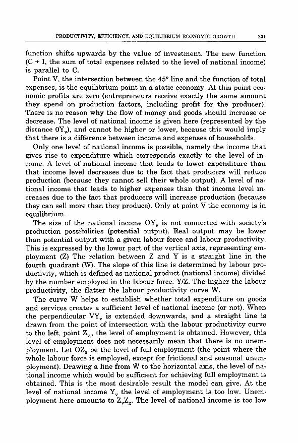
function shifts upwards by the value of investment. The new function (C + I, the sum of total expenses related to the level of national income) is parallel to C.

Point V, the intersection between the 45° linę and the function of total expenses, is the equilibrium point in a static economy. At this point eco- nomic profits are zero (entrepreneurs receive exactly the same amount they spend on production factors, including profit for the producer). There is no reason why the flow of money and goods should increase or decrease. The level of national income is given here (represented by the distance 0Yv), and cannot be higher or lower, because this would imply that there is a difference between income and expenses of households.

Only one level of national income is possible, namely the income that gives rise to expenditure which corresponds exactly to the level of in­come. A level of national income that leads to lower expenditure than that income level decreases due to the fact that producers will reduce production (because they cannot sell their whole output). A level of na­tional income that leads to higher expenses than that income level in- creases due to the fact that producers will increase production (because they can sell morę than they produce). Only at point V the economy is in eąuilibrium.

The size of the national income OYV is not connected with society’s production possibilities (potential output). Real output may be lower than potential output with a given labour force and labour productivity. This is expressed by the lower part of the vertical axis, representing em- ployment (Z) The relation between Z and Y is a straight linę in the fourth quadrant (W). The slope of this linę is determined by labour pro- ductivity, which is defined as national product (national income) divided by the number employed in the labour force: Y/Z. The higher the labour productivity, the flatter the labour productivity curve W.

The curve W helps to establish whether total expenditure on goods and services creates a sufficient level of national income (or not). When the perpendicular VYv is extended downwards, and a straight linę is drawn from the point of intersection with the labour productivity curve to the left, point Zv, the level of employment is obtained. However, this level of employment does not necessarily mean that there is no unem- ployment. Let OZX be the level of fuli employment (the point where the whole labour force is employed, except for frictional and seasonal unem- ployment). Drawing a linę from W to the horizontal axis, the level of na­tional income which would be sufficient for achieving fuli employment is obtained. This is the most desirable result the model can give. At the level of national income Yv the level of employment is too Iow. Unem- ployment here amounts to ZVZX. The level of national income is too Iow

232 JÓZEF JAGAS

as well (Yv is smaller than potential output, Yx). Why? Because total ex- penditures are too Iow (only VYv). Total expenditures should be XYx, in order to obtain the optimal level of national income. Thus V is the ‘false eąuilibrium’ and X the ‘true eąuilibrium’. The ‘false eąuilibrium’, the cause of unemployment and too Iow a national income is a conseąuence of the fact that XYx - VYv is missing in C + I. This is called demand defi- ciency or a deflationary gap.2 If the C + I curve took another position, ac- cording to the model would there would be an inflationary gap. These gaps are the villains: when we want to have a happy end, it is necessary to eliminate them. In this case this is a task of the government. Govern- ment policy should highlight the elimination of the gap between actual expenses and the socially necessary level of expenses.

2 This term is also used in a different sense, namely as a sign of an initial incentive necessary to eliminate the lack of aggregate demand. P.A. Samuelson, for example, ap- plies the term in this sense. This gap is smaller than ours; the ratio between them is equal to the multiplier. I prefer my own definition, because it is easier to calculate the absolute lack of demand than incentives which, according to us, may eliminate this lack. In practice it is not possible to accurately calculate the multiplier [J. Pen, in Jagas, J., op. cit., p. 111].

Proper government policy leads to an increase in national income. An effective way to achieve this is not only an upward shift of the curve of total expenditure, but also its rotation. When the curve rotates in such a way that the angle is closer to the 45° linę, the eąuilibrium point V can shift rightwards strongly, causing a spontaneous increase in income. The ‘false eąuilibrium’, V settles at the right of the ‘true eąuilibrium’. When drawing a straight linę downwards, it can be observed that a point is achieved on the Z-axis, which lies below Zx. This means that the demand for labour exceeds its supply. The monetary national income becomes too large, and tensions appear in the national economy. Morę goods are needed than firms can produce. This is the inflationary gap, which can be analysed in the diagram in a similar way as the deflationary gap.

It has to be mentioned that an increase in labour productivity is shown in this model by a flatter curve W, causing point X to shift up- wards to the right, further away from point V. This would make the de­mand deficiency morę severe.

In order to capture the influence of labour productivity on the level of national product (income) - being its regulator - a dynamie model should be applied, for example of the Harrod-Domar type. In such a model the relationship between labour productivity and the scalę of Capital growth (investment) necessary for achieving higher eąuilibrium income can be grasped.

PRODUCTIYITY, EFFICIENCY, AND EQUILIBRIUM ECONOMIC GROWTH 233

The dynamie model

The static model presented above contains assumptions which have to be dropped when making a long-term analysis. Among other things, a departure from the simplification that consumption can be described by the formula C = A + cY, where A and c are constants, is essential. This is shown in Figurę 2. Furthermore, changes in productivity through time must be allowed for.

Fig. 2. A dynamie model of production, consumption, and labour productivity

When the economy is at equilibrium, i.e. moving along the linę 0X, an inerease in national income from Yv to Yx has to be accompanied by an appropriate inerease in investment I, which is shown by the lines VF and XG. When the share of investment in national income is compared, i.e. when the ratios VF/VD and XG/XH are calculated, it can be stated that growth of consumption according to the formula C = A + cY means that growth of Y reąuires a constant inerease in the investment share in national income, which is equivalent to the decrease of the share of con­sumption in national income to zero.

In Figurę 2 an additional linę of labour productivity (W2), which would ensure fuli employment at a level of national income Yv, is drawn. This can hardly be regarded as an interesting solution, for this would mean a decrease in labour productivity from W1 to W2. In order to show which changes in labour productivity can ensure fuli utilisation of the la-

234 JÓZEF JAGAS

bour force in a market economy, new assumptions have to be introduced, which make it possible to capture those elements that in the long-run have the most significant influence on economic growth. For this pur- pose the following assumptions are adopted:1. The eąuilibrium market economy is analysed, in which the expendi-

ture on consumption and investment equal the value of the national product (income), i.e. the following condition is fulfilled:

C + I = Y

This means that there is only movement along the linę X in Figurę 2.2. The possibility of substitution between labour and Capital is repre-

sented by the production isocline (production curve), specified for the initial level of production Yo in period t by the formula:

Z = atK-a (1)

Where K is Capital, and at and a are constans larger than zero.

3. There are constant returns to scalę, i.e. the size of national income Y increases at the same ratę as Z and K when the same production method is used.3

4. Investment is only financed from profits and immediately increases the amount of Capital. The part of national income that is not invested is consumed.

3Two methods are the same, when they are characterised by identical Capital and la­bour intensity (Forlicz, S., Jagas, J., Jasiński, M., and Linek, S., Wydajność pracy jako regulator produkcji, Opole, 1995).

‘Labour friendly’ economic growth in the dynamie model

Technological progress, understood in a broad sense has always been a factor that has sąueezed out labour, thus being a real or potential threat for inereasing unemployment. As an illustration, data concerning eco­nomic growth in the European Union (as a whole) between 1974 and 1997 are used. During this period the average labour productivity inereased by about 2% per year. It has been estimated that about half of this growth (1%) was the result of scientific, technical, and organisational progress. The other half, however, was the result of the substitution of labour for Capital at a given level of production technology. At the same time the av-

PRODUCTIYITY, EFFICIENCY, AND EQUILIBRIUM ECONOMIC GROWTH 235

erage yearly increase in labour productivity was 0.7% in the USA, while Japan with 1.9% experienced a growth ratę similar to the EU.4

4 Fiodor, B., “«Pracoprzyjazny» wzrost gospodarczy — próba ujęcia teoretycznego i rela­cje do polityki płac i zatrudnienia”, [in:] Produktywność, Integracja, J. Jagas (ed.), Opole, 1999, pp. 50-51.

5 Data from: Growth and employment in the stability - oriented framework of EMU, Eu­ropean Commission, Brussels, 1998.

The growth of labour productivity in the EU was accompanied by in- creasing unemployment, although with variable dynamics, from about 5% at the beginning of the 1960s to 10.7% in 1997. At the same time the proportion of people professionally active fell from 67% to 61% (while currently 74% of the total population in Japan and USA are profession­ally active).5 Thus the price for the high growth of labour productivity in Europę was a significant increase in the unemployment level. On the other hand, without increasing labour productivity when there was a fast increase in wages and welfare benefits (non-wage labour costs), the countries of the European Union would not be able to keep up with the challenges of stronger competition on International markets.

According to standard neo-classical growth theory, there will be fuli employment of available labour when the growth level is eąual to the sum of the exogenously given level of population growth and the level of technological progress. The latter should have a elear ‘labour augment- ing’ character, i.e. be neutral in the sense of Harrod’s definition. In other words, growth with fuli employment, i.e. the realisation of the so-called natural growth ratę, reąuires that the growth ratę of labour productivity exactly equals the growth ratę of labour sources. Implicitly this means an increase in the amount of labour, both in the natural sense and the ‘unit efficiency’ sense (this is essentially caused by ‘labour augmenting’ of technological progress) and the non-appearance of substitution of la­bour for Capital at a given level of production technology. In theory, the second process will be counteracted - in a quantitative sense — by the appropriate degree of substitution elasticity between labour and Capital. This especially concerns the situation where the elasticity equals one. This means that the ratio between prices of production factors changes in the opposite direction, but quantitatively, taking the modulus, exactly like the ratio between the quantities of production factors. Thus, for in- stance, the relative growth (in relation to Capital) saturating the econ- omy with labour will be accompanied by an opposite (but alike with re- spect to absolute value) change in the prices ratio of production factors (labour to Capital).

236 JÓZEF JAGAS

Generalising the above theoretical considerations a little, it can be said that ‘labour friendly’ economic growth requires the existence of elas- tic and completely competitive markets for production factors. The lack of such elasticity and competitiveness can stimulate the pace of substitu- tion of labour for Capital in such a way, that even under the condition of an increase in supply of Capital part of the labour supply cannot find em- ployment.

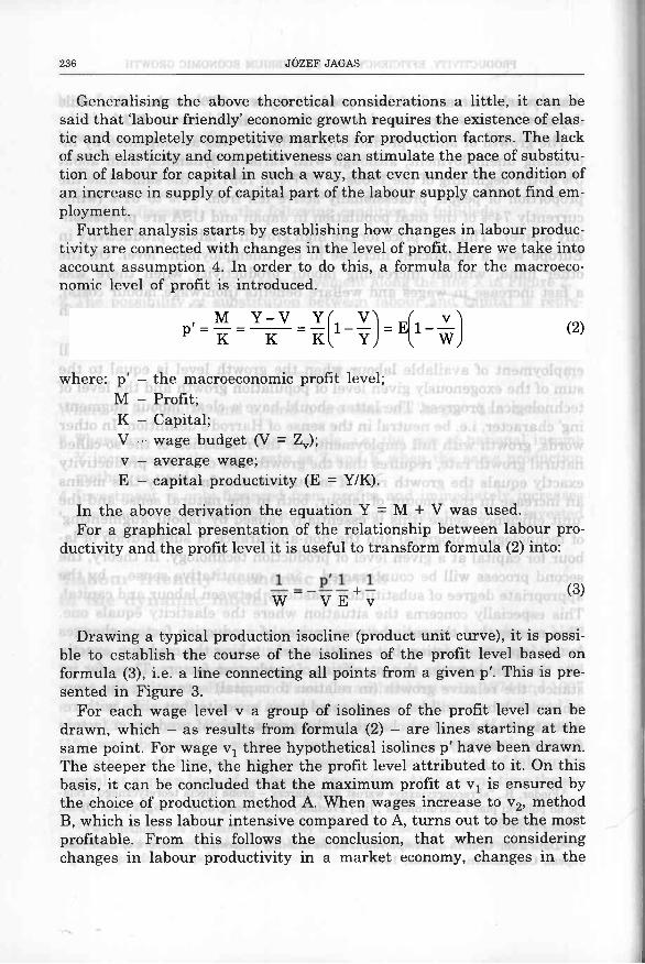
Further analysis starts by establishing how changes in labour produc- tivity are connected with changes in the level of profit. Here we take into account assumption 4. In order to do this, a formula for the macroeco- nomic level of profit is introduced.

where: p' — the macroeconomic profit level;M - Profit;K - Capital;V - wagę budget (V = Zv);v - average wagę;E - Capital productivity (E = Y/K).

In the above derivation the eąuation Y = M + V was used.For a graphical presentation of the relationship between labour pro-

ductivity and the profit level it is useful to transform formula (2) into:

W"’VE + v (3)

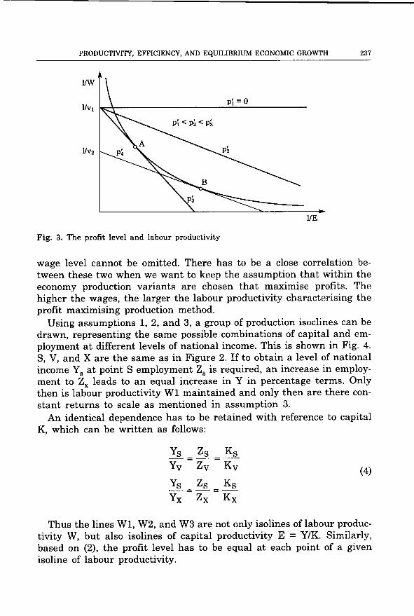
Drawing a typical production isocline (product unit curve), it is possi- ble to establish the course of the isolines of the profit level based on formula (3), i.e. a linę connecting all points from a given p'. This is pre- sented in Figurę 3.

For each wagę level v a group of isolines of the profit level can be drawn, which - as results from formula (2) - are lines starting at the same point. For wagę Vj three hypothetical isolines p' have been drawn. The steeper the linę, the higher the profit level attributed to it. On this basis, it can be concluded that the maximum profit at V! is ensured by the choice of production method A. When wages increase to v2, method B, which is less labour intensive compared to A, turns out to be the most profitable. From this follows the conclusion, that when considering changes in labour productivity in a market economy, changes in the

PRODUCTIYITY, EFFICIENCY, AND EQUILIBRIUM ECONOMIC GROWTH 237

Fig. 3. The profit level and labour productivity

wagę level cannot be omitted. There has to be a close correlation be- tween these two when we want to keep the assumption that within the economy production variants are chosen that maximise profits. The higher the wages, the larger the labour productivity characterising the profit maximising production method.

Using assumptions 1, 2, and 3, a group of production isoclines can be drawn, representing the same possible combinations of Capital and em- ployment at different levels of national income. This is shown in Fig. 4. S, V, and X are the same as in Figurę 2. If to obtain a level of national income Ys at point S employment Zs is required, an increase in employ- ment to Zx leads to an equal increase in Y in percentage terms. Only then is labour productivity W1 maintained and only then are there con- stant returns to scalę as mentioned in assumption 3.

An identical dependence has to be retained with reference to Capital K, which can be written as follows:

Ys.= Z^= Kg.Yv Zv Kv

Ys = Zs =JkYx Zx Kx

Thus the lines Wl, W2, and W3 are not only isolines of labour produc- tivity W, but also isolines of Capital productivity E = Y/K. Similarly, based on (2), the profit level has to be equal at each point of a given isoline of labour productivity.

238 JÓZEF JAGAS

Fig. 4. A group of production isoclines

In the static model, point S represents a simple reproduction economy, where no new investments take place. Total national income is consumed here. In order to achieve national income Yv, social expenditures have to increase with investment,6 which not only increases aggregate demand, but also increases the production possibilities from the side of Capital. Complete use of the labour force would reąuire an increase of employment to Zx, which entails an increase in Y by the same percentage as the in­crease in Z. In order to keep labour productivity at the previous level, Cap­ital K has to increase in a similar way. Investments are indispensable in order to achieve this. The size of investment that is needed to go from point S to V, X, or L in Figurę 4 can be obtained by subtracting Ks from the amount of Capital attributed to each of these points.7 Fuli employment can also be achieved without new investments. It is sufficient that labour productivity decreases to W2, which, for example, can be achieved by structural economic changes increasing the share of labour-intensive ac- tivities in the economy. It is also possible to increase Capital to KL, caus- ing labour productivity to increase to W3.

6 In Figurę 2 this is shown by the distance VF and in Figurę 3 by the distance E.7 At this moment a problem appears, of which only an indication can be given in this

paper. Investment causes the production possibilities to increase by the same percentage as Capital increases. At the same time, this investment creates additional demand. If the consumption were described by the formula from the static model, only in one case can the economy remain on the linę 0X in Figurę 2. In all other cases the productive forces of the economy would grow too fast or too slow in relation to the increase in expenses (de­mand). This is also a reason why it was necessary to drop the assumption that C = A + cY.

In order to state what is the relationship between labour productivity and national income, at the beginning the following relationship should be

PRODUCTIVITY, EFFICIENCY, AND EQUILIBRIUM ECONOMIC GROWTH 239

recalled: Y = Z W. When further anałysis is limited to only those variants that realise fuli employment, i.e. where Z is given and amounts to Zx, the growth of Y depends on W. Based on Figurę 4 it can be argued that for a given Z, labour productivity increases with K. The morę investment, the morę Capital. Investment cannot rise freely, because consumption con- straints do not allow it. In order to get a better view of the described rela- tionships, a simulation of the calculations will be carried out. In this way it is easier to show the active constraints on an increase in W and Y.

Let us assume that the starting point S of the economy is character- ised by the following initial data: Yg = 1, a = 1, a = 4, vs = 0.25. Applying the assumptions of the model, it can be proven that profit is maximised when the following condition is fulfilled:8

8 The derivation of this formula can, among others, be found in: Jasiński, M., “Postęp techniczny w funkcji produkcji Cobba-Douglasa”, Ekonomista 1994, no. 1, pp. 91-92.

9Ibid., p. 89. It can be observed that this function is a special type of the Cobb-Douglas function.

Wmaxp'=(a+1) <5)

In order to obtain a starting point, which is a stable eąuilibrium, it has to be assumed that Ws and, at the same time, Zs = 2. On the basis of formula (1), it can be calculated that Ks = 2. Using the data above we get: Vs = 0.5, Ms = 0.5, and Es = 0.5. The initial level of profit will amount to p's = 0.25. This is the maximum profit that can be achieved. Additionally, it is assumed that the number of people willing to work amounts to Zx = 2.5.

First the case where there are no new investments, and nevertheless the aim is to achieve fuli employment. In period t Capital will be the same as at the point S, i.e.: Kj = Ks = 2. Using formula (1) and assump- tion 3, the following production function can be derived:9

Yt = Ysa-V(«+1)zy(a+1)K“/(a+1) (6)

The level of employment is also determined: Zt = Zx = 2.5. This leads to achieving a national income of 1.118. At the same time the labour pro- ductivity declines from 0.5 to 0.447. According to formula (5) wages also must decline to 0.224. Wagę budget V amounts to 0.559 and profit M is equal to 0.559. The whole profit will be consumed, i.e. C = 1.118. The level of profit increases to 0.279.

Now let us consider a second extreme case, assuming that the whole profit madę in period t will be invested. The size of M depends on the size of Y,

240 JÓZEF JAGAS

which is significantly affected by the size of K, which again depends on M. When the following condition for maximising the level of profit is added:10

10Ibid., p. 92.

vY/maxp’ a+1

it can be argued that Kt is a function of Yt:

OtKt=Ks+It = Ks+Mt=Ks +------Yt (8)a+1

Substituting (8) into (6) and solving, we get Yt = 1.285. This implies that labour productivity is 0.514, while, at the same time, wages have to rise to 0.257. The wagę budget is 0.643 and eąuals profit M. Capital in- creases to 2.643 and the profit level decreases to 0.243. The largest dif- ference with the first case can be observed in the level of consumption. Consumption now only responds to V, for which reason C = 0.643 instead of 1.118.

Finally, an intermediate case is considered, assuming that wages and labour productivity do not change, i.e. will be the same as at point S. When W is constant, an increase in employment from 2 to 2.5 causes an increase of Yt to 1.25, while both the wagę budget and profit will amount to 0.625. Capital will be equal to 2.5. This means that 0.125 from the profit is assigned to consumption. Aggregate consumption thus amounts to 0.75. The profit level stays on the previous level of 0.25.

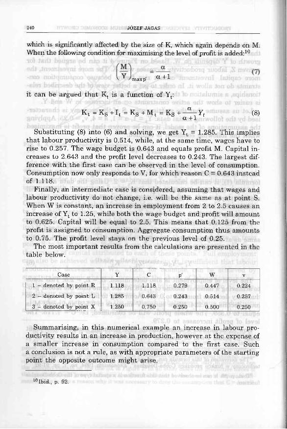
The most important results from the calculations are presented in the table below.

Case Y C P' W V

1 - denoted by point R 1.118 1.118 0.279 0.447 0.2242 - denoted by point L 1.285 0.643 0.243 0.514 0.2573 - denoted by point X 1.250 0.750 0.250 0.500 0.250

Summarising, in this numerical example an increase in labour pro- ductivity results in an increase in production, however at the expense of a smaller increase in consumption compared to the first case. Such a conclusion is not a rule, as with appropriate parameters of the starting point the opposite outcome might arise.