49
Kalman Filter

Kalman Filter
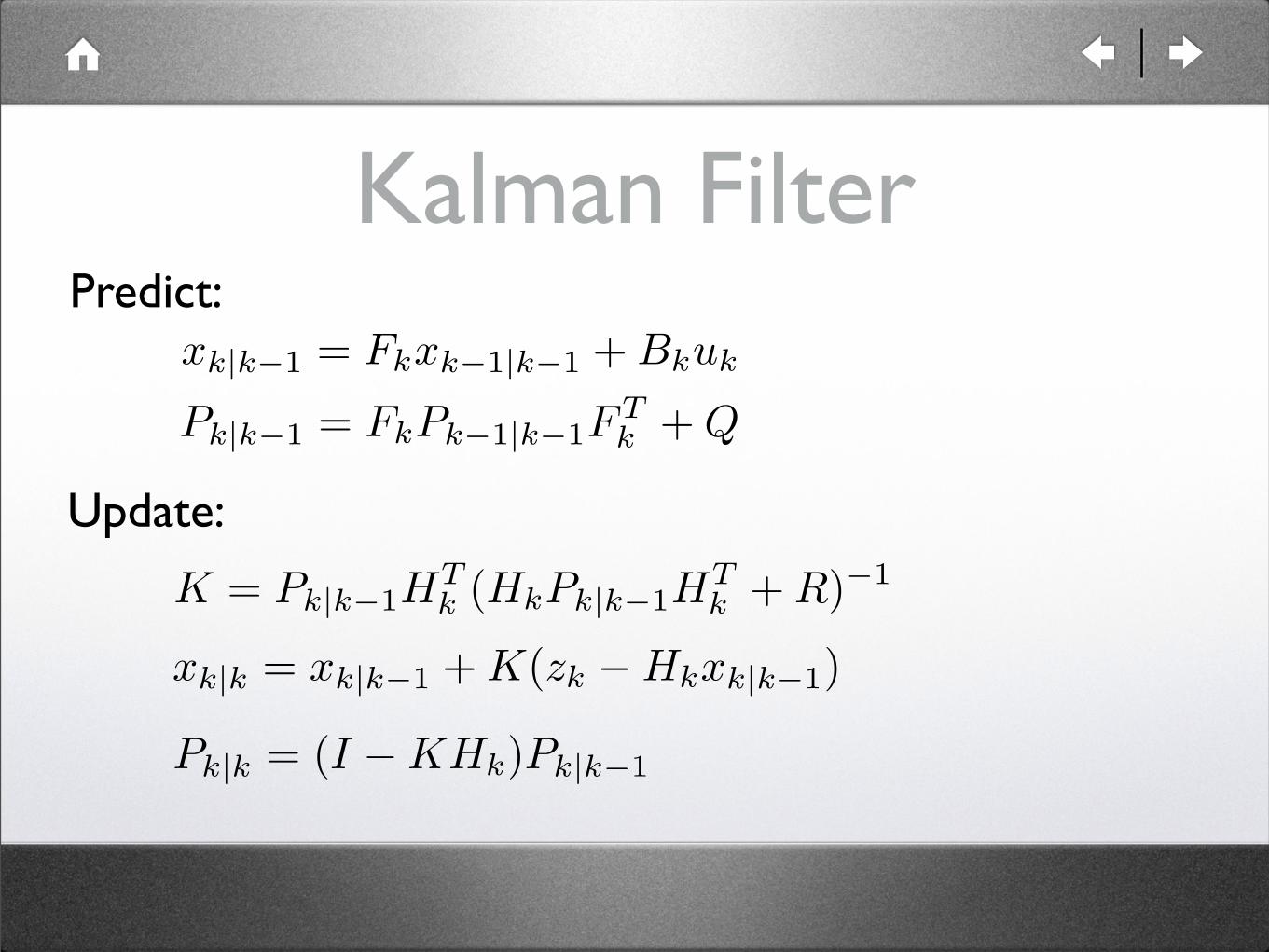
Kalman FilterPredict:
Update:
xk|k−1 = Fkxk−1|k−1 + Bkuk
Pk|k−1 = FkPk−1|k−1FTk + Q
K = Pk|k−1HTk (HkPk|k−1H
Tk + R)−1
xk|k = xk|k−1 + K(zk −Hkxk|k−1)
Pk|k = (I −KHk)Pk|k−1
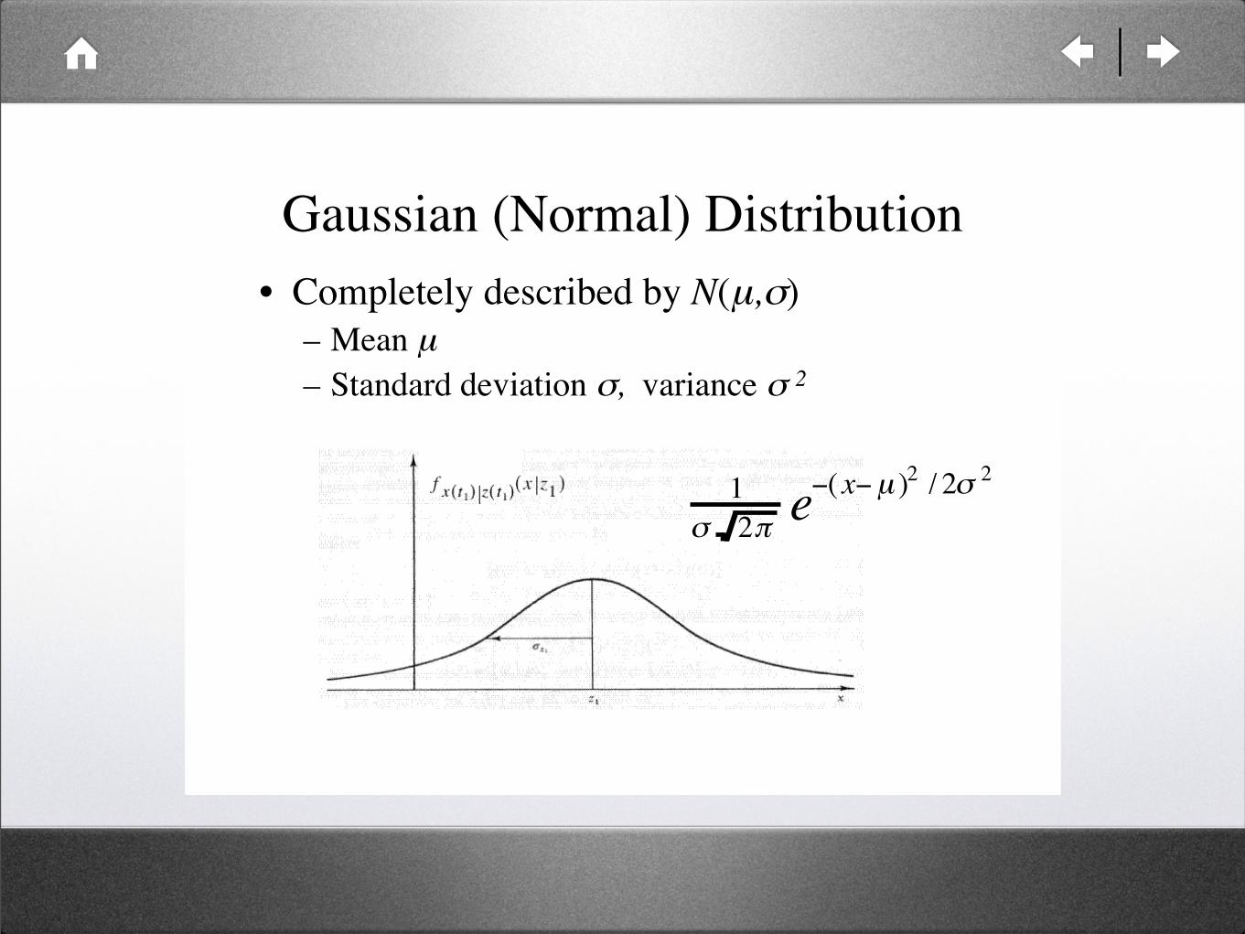
Gaussian (Normal) Distribution
• Completely described by N(µ,!)
– Mean µ
– Standard deviation !, variance ! 2
!
1
" 2#e$( x$µ )2 / 2" 2
The Central Limit Theorem
• The sum of many random variables
– with the same mean, but
– with arbitrary conditional density functions,
converges to a Gaussian density function.
• If a model omits many small unmodeled
effects, then the resulting error should
converge to a Gaussian density function.
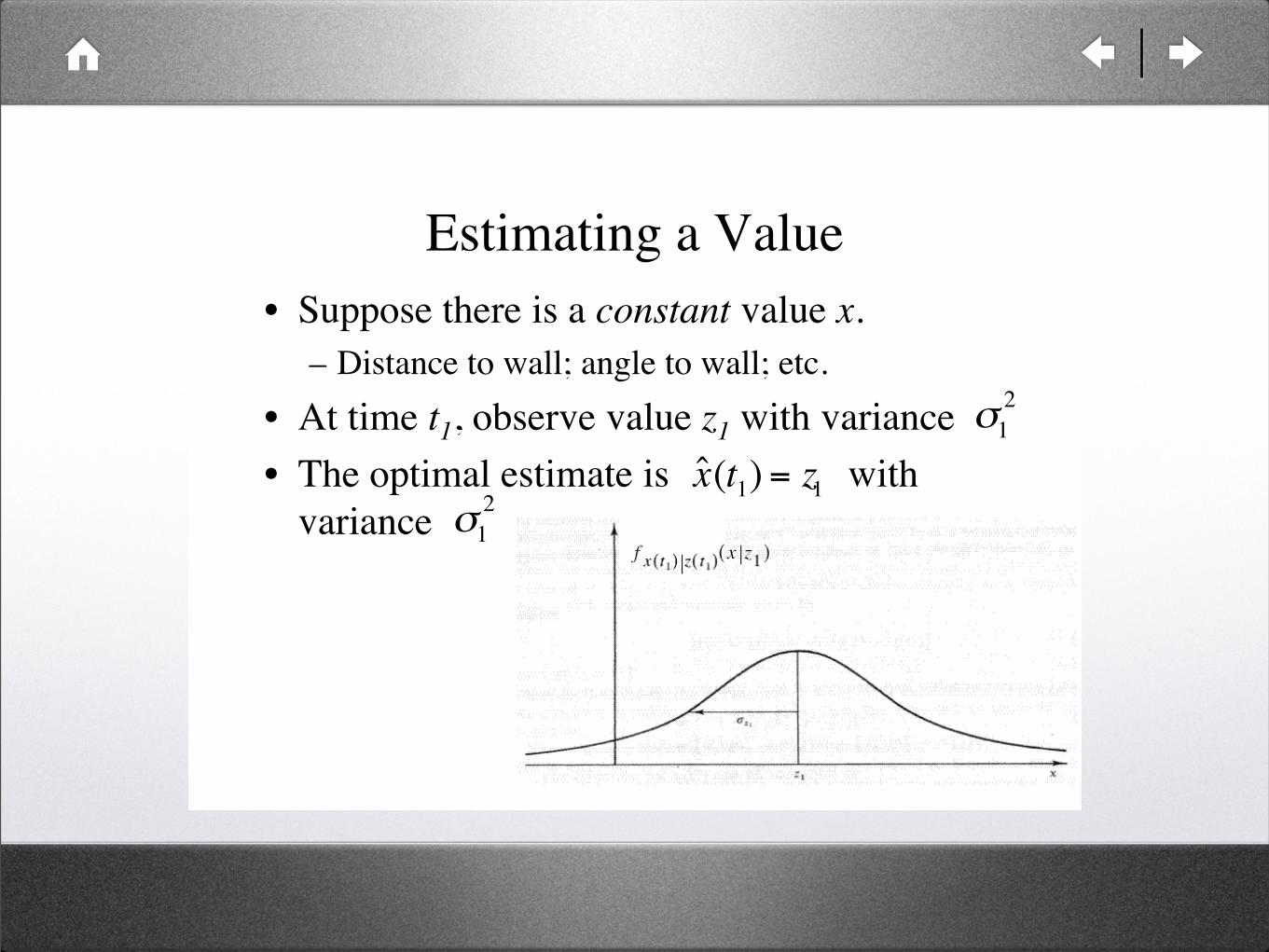
Estimating a Value
• Suppose there is a constant value x.
– Distance to wall; angle to wall; etc.
• At time t1, observe value z1 with variance
• The optimal estimate is with
variance
!
"1
2
!
ˆ x (t1) = z
1
!
"1
2
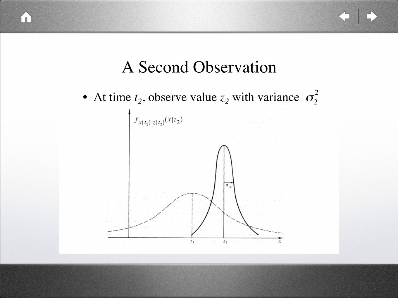
A Second Observation
• At time t2, observe value z2 with variance
!
"2
2
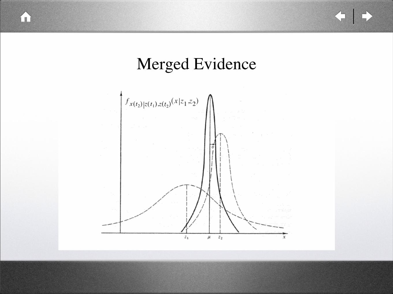
Merged Evidence
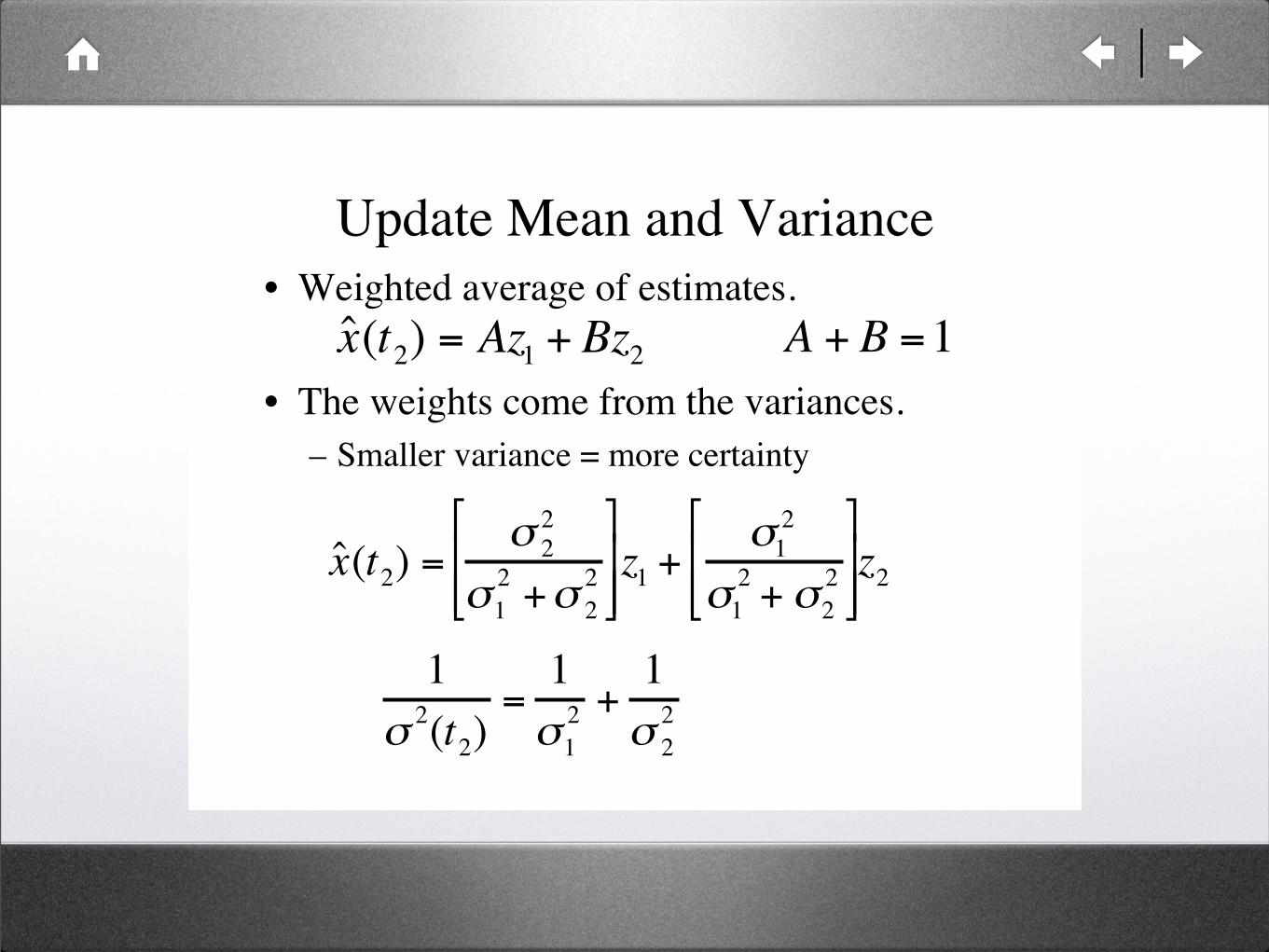
Update Mean and Variance
• Weighted average of estimates.
• The weights come from the variances.
– Smaller variance = more certainty
!
ˆ x (t2) = Az
1+ Bz
2
!
ˆ x (t2) =
"2
2
"1
2+"
2
2
#
$ % %
&
' ( ( z
1+
"1
2
"1
2+ "
2
2
#
$ % %
&
' ( ( z
2
!
1
"2(t2)
=1
"1
2+1
"2
2
!
A + B =1
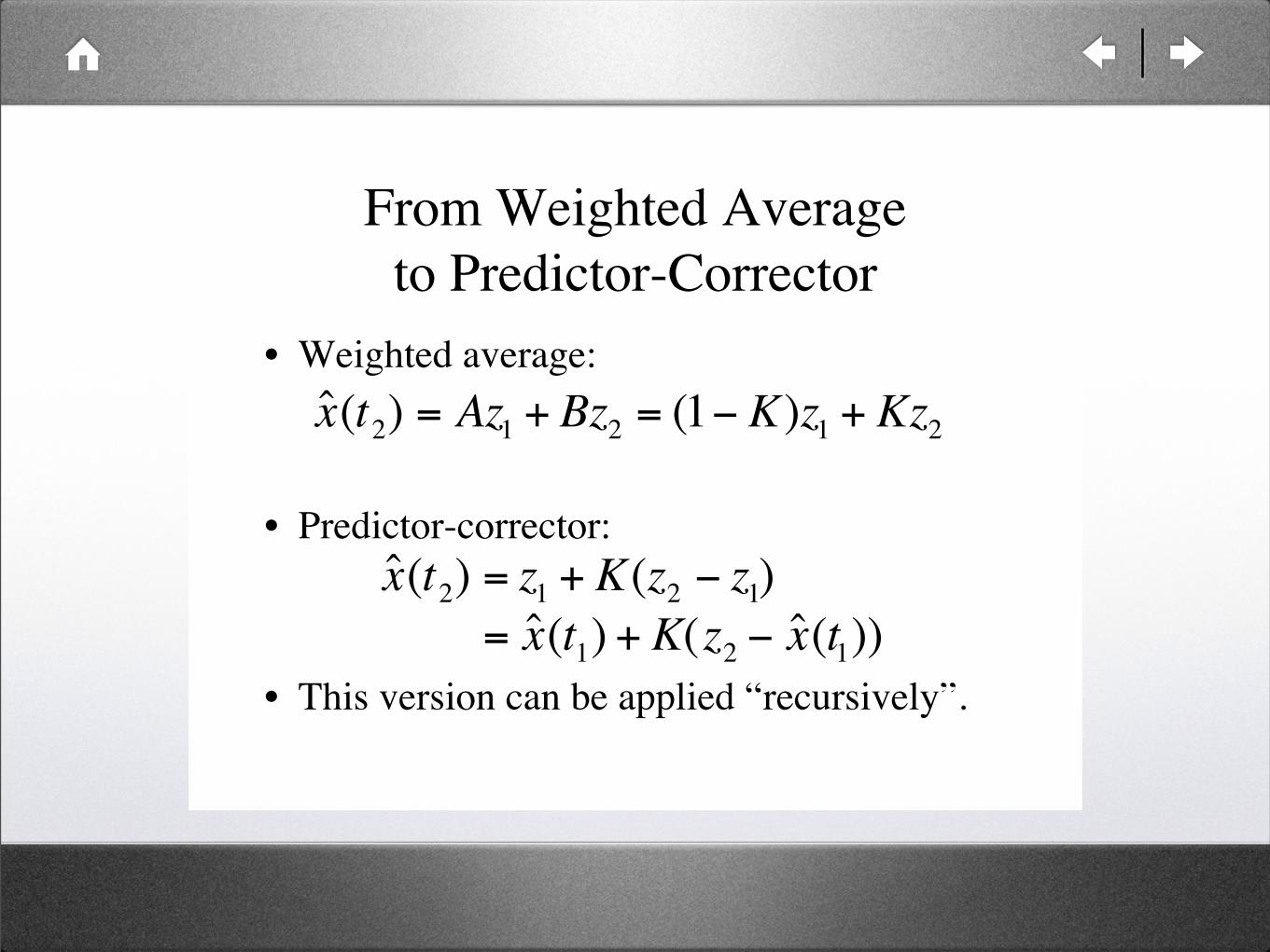
From Weighted Average
to Predictor-Corrector
• Weighted average:
• Predictor-corrector:
• This version can be applied “recursively”.
!
ˆ x (t2) = Az
1+ Bz
2= (1" K)z
1+ Kz
2
!
ˆ x (t2) = z
1+ K(z
2" z
1)
!
= ˆ x (t1) + K(z
2" ˆ x (t
1))
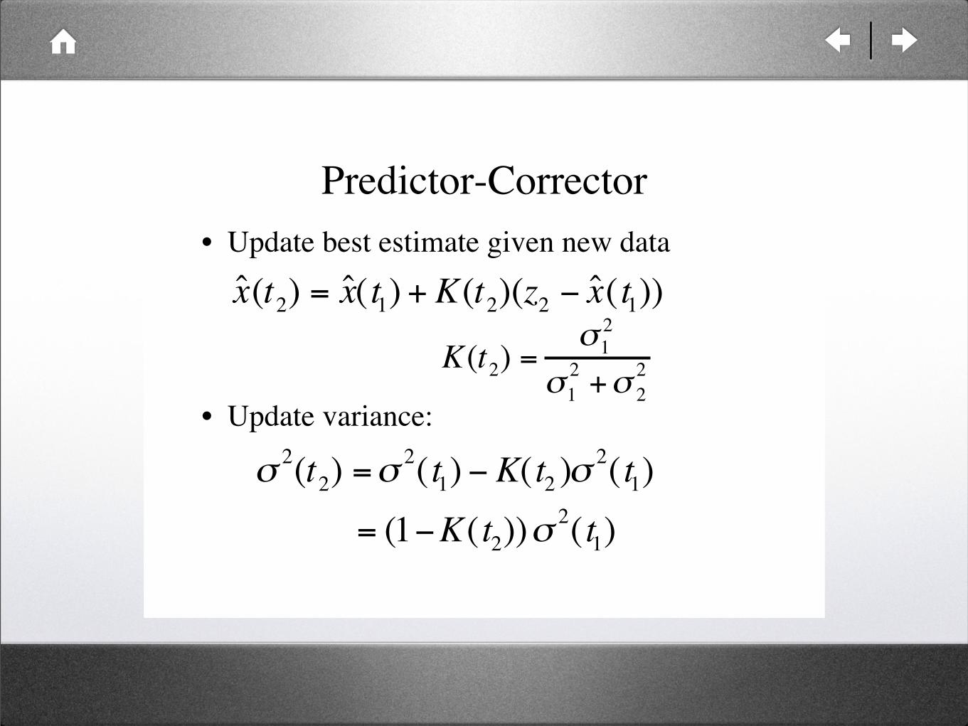
Predictor-Corrector
• Update best estimate given new data
• Update variance:
!
ˆ x (t2) = ˆ x ( t
1) + K(t
2)(z
2" ˆ x ( t
1))
!
K(t2) =
"1
2
"1
2+"
2
2
!
"2(t2) ="
2( t1) # K(t
2)"
2( t1)
!
= (1"K( t2))#
2( t1)
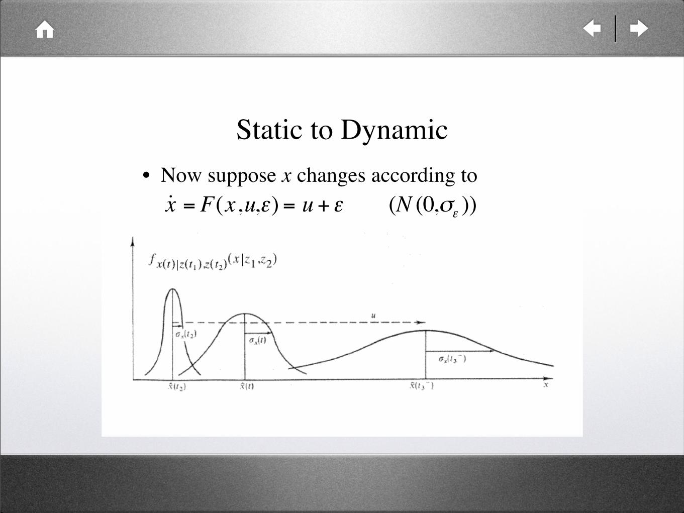
Static to Dynamic
• Now suppose x changes according to
!
˙ x = F(x,u,") = u +" (N (0,#" ))
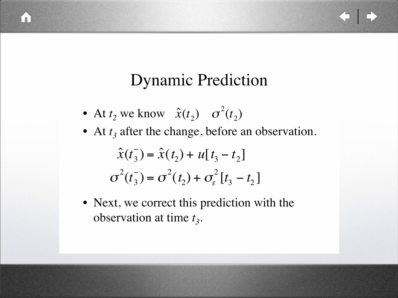
Dynamic Prediction
• At t2 we know
• At t3 after the change, before an observation.
• Next, we correct this prediction with the
observation at time t3.
!
ˆ x (t3
") = ˆ x ( t
2) + u[ t
3" t
2]
!
"2(t3
#) = "
2( t2) + "$
2[t3# t
2]
!
ˆ x (t2) "
2(t
2)
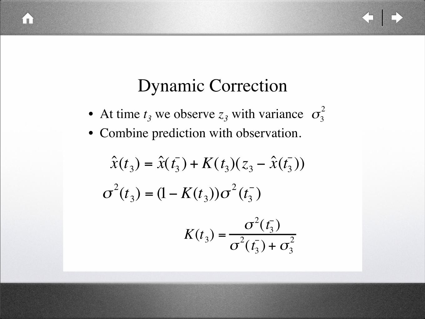
Dynamic Correction
• At time t3 we observe z3 with variance
• Combine prediction with observation.
!
"3
2
!
ˆ x (t3) = ˆ x ( t
3
") + K( t
3)(z
3" ˆ x (t
3
"))
!
K(t3) =
" 2( t3
#)
"2( t3
#) + "
3
2
!
"2(t3) = (1# K(t
3))"
2(t3
#)
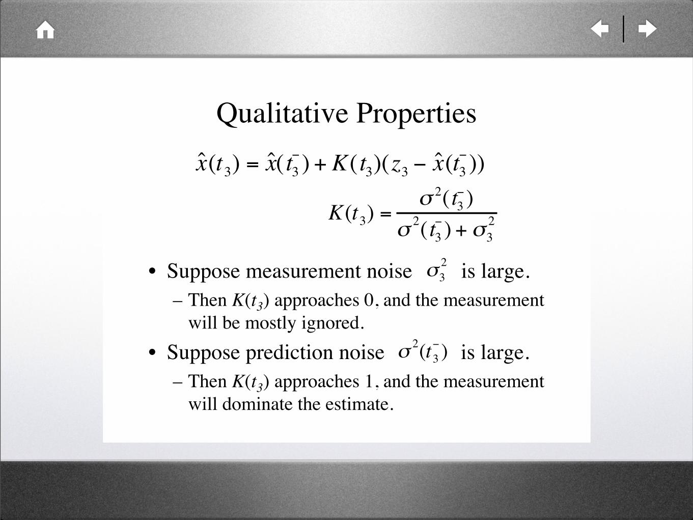
Qualitative Properties
• Suppose measurement noise is large.
– Then K(t3) approaches 0, and the measurement
will be mostly ignored.
• Suppose prediction noise is large.
– Then K(t3) approaches 1, and the measurement
will dominate the estimate.
!
K(t3) =
" 2( t3
#)
"2( t3
#) + "
3
2
!
ˆ x (t3) = ˆ x ( t
3
") + K( t
3)(z
3" ˆ x (t
3
"))
!
"3
2
!
"2(t3
#)
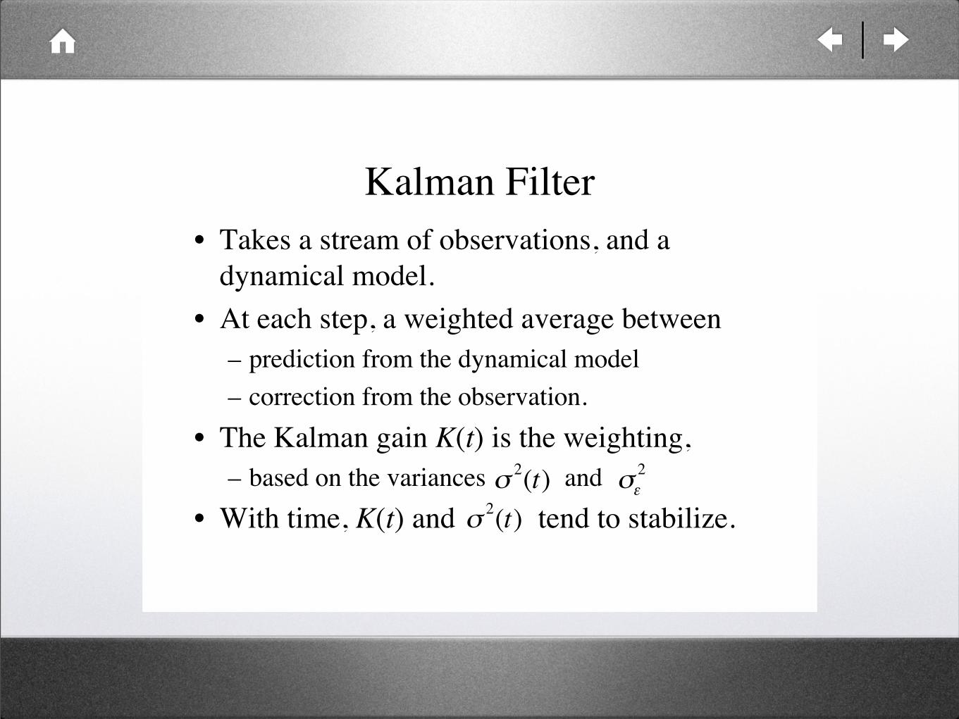
Kalman Filter
• Takes a stream of observations, and a
dynamical model.
• At each step, a weighted average between
– prediction from the dynamical model
– correction from the observation.
• The Kalman gain K(t) is the weighting,
– based on the variances and
• With time, K(t) and tend to stabilize.
!
"2(t)
!
"#2
!
"2(t)
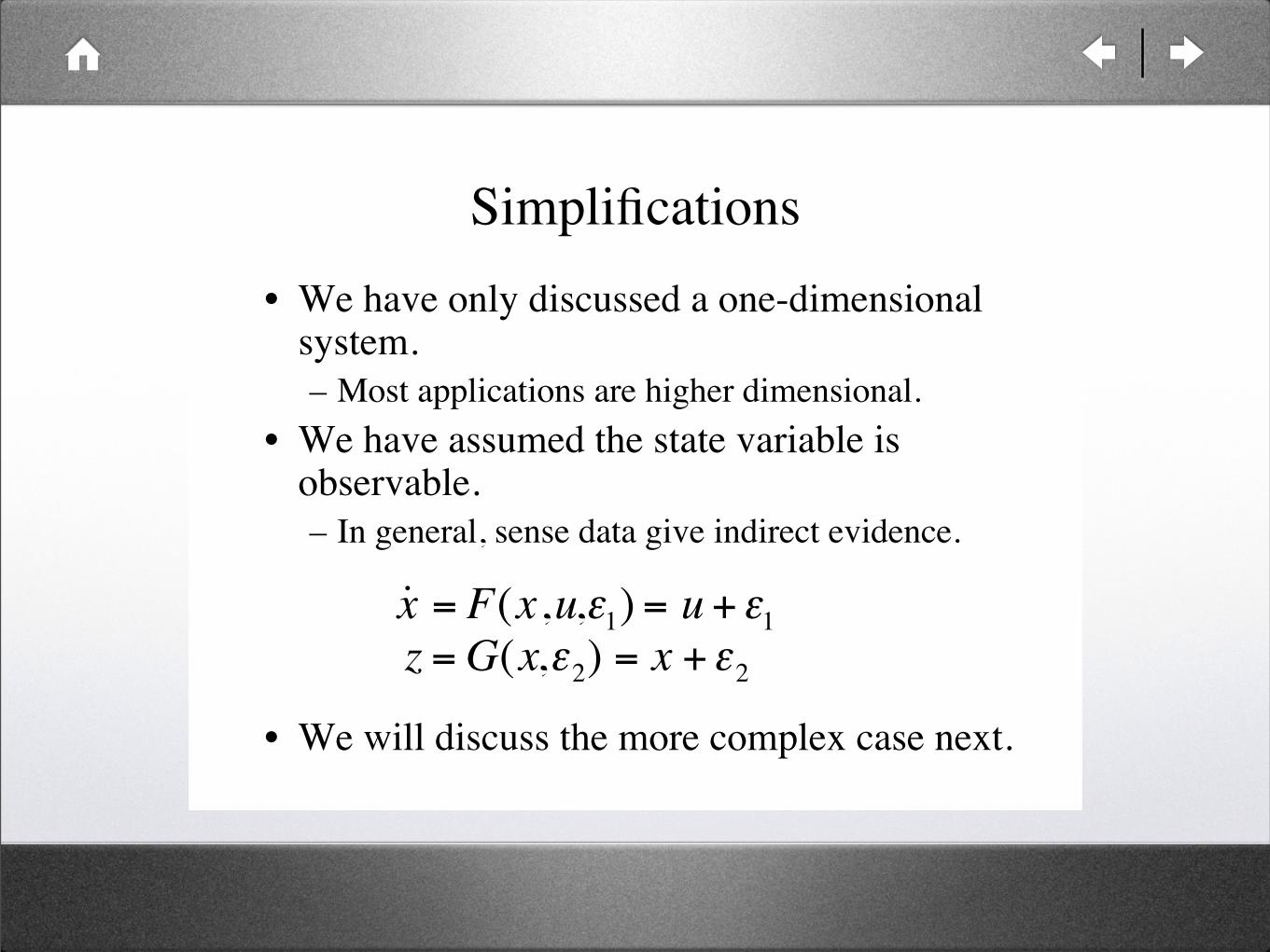
Simplifications
• We have only discussed a one-dimensionalsystem.
– Most applications are higher dimensional.
• We have assumed the state variable isobservable.
– In general, sense data give indirect evidence.
• We will discuss the more complex case next.
!
˙ x = F(x,u,"1) = u +"
1
!
z =G(x,"2) = x +"
2
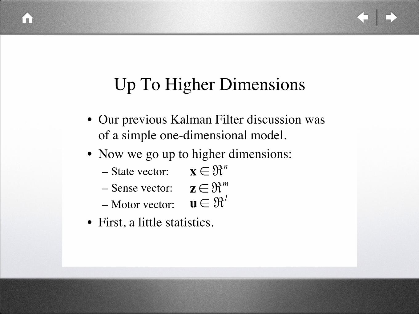
Up To Higher Dimensions
• Our previous Kalman Filter discussion was
of a simple one-dimensional model.
• Now we go up to higher dimensions:
– State vector:
– Sense vector:
– Motor vector:
• First, a little statistics.
!
x "#n
!
z "#m
!
u" #l
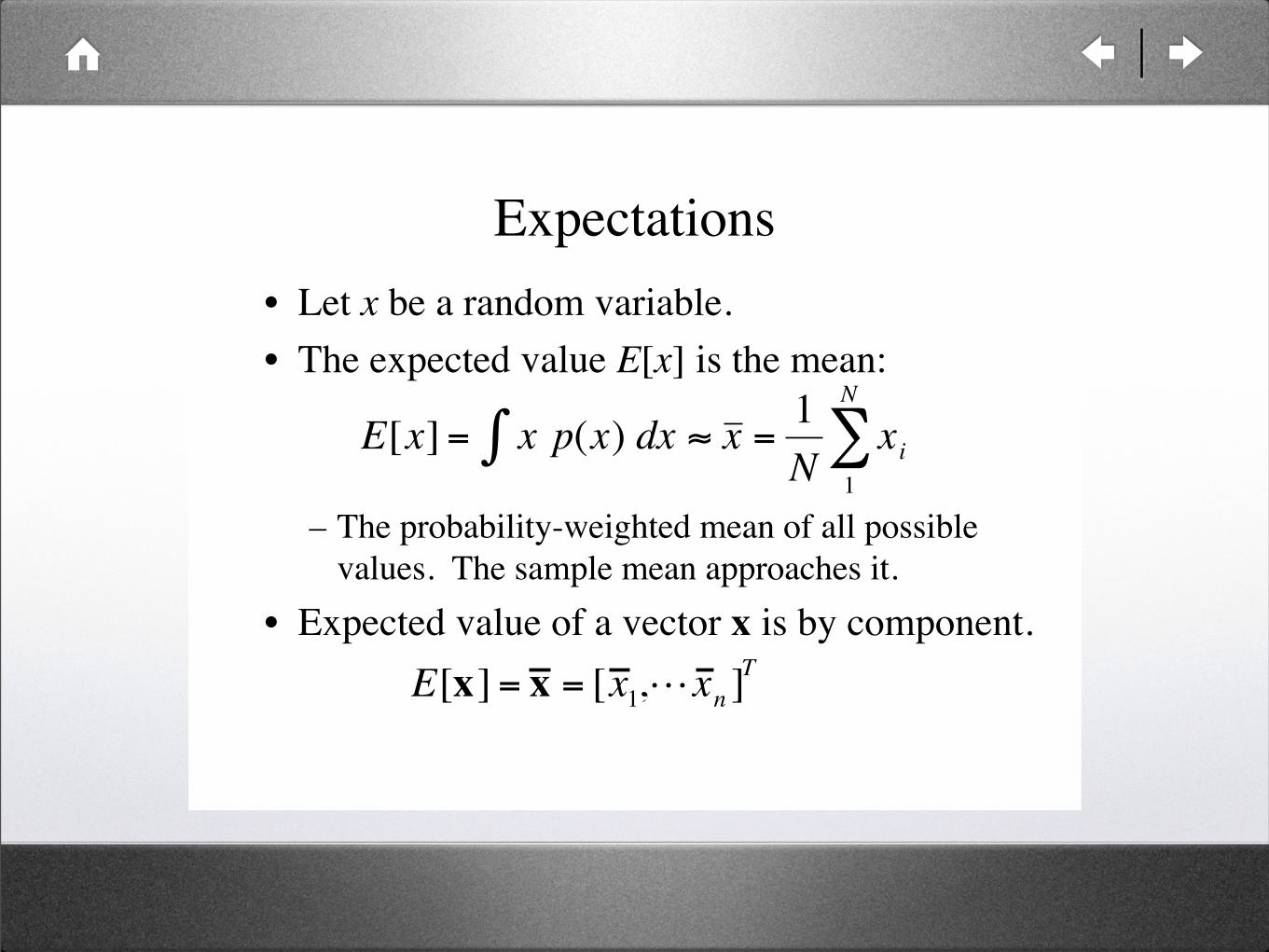
Expectations
• Let x be a random variable.
• The expected value E[x] is the mean:
– The probability-weighted mean of all possible
values. The sample mean approaches it.
• Expected value of a vector x is by component.!
E[x] = x p(x) dx" # x =1
Nxi
1
N
$
!
E[x] = x = [x 1,Lx
n]T
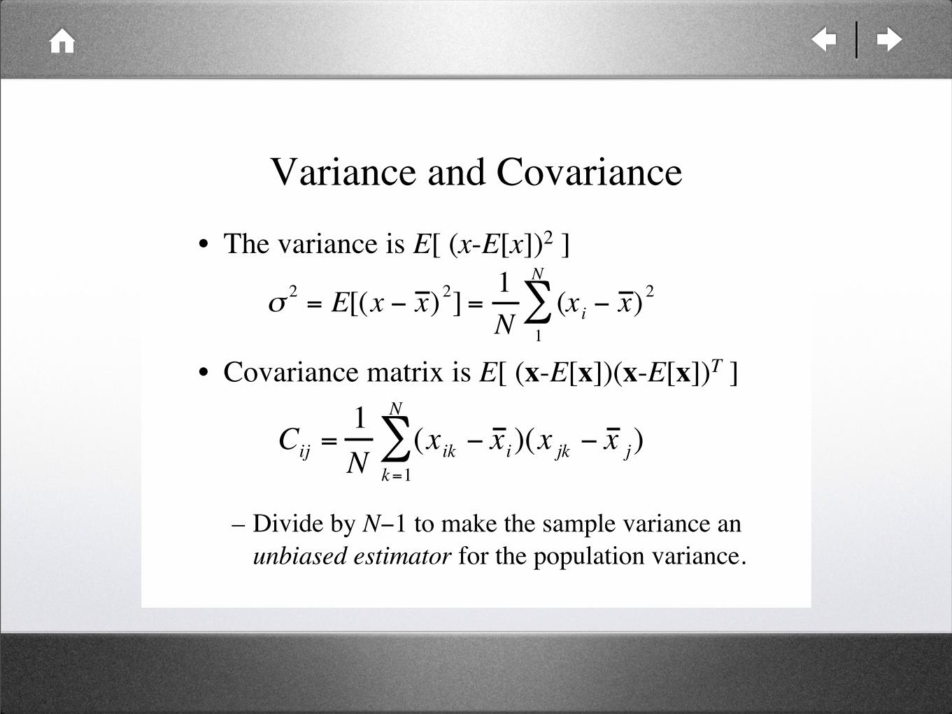
Variance and Covariance
• The variance is E[ (x-E[x])2 ]
• Covariance matrix is E[ (x-E[x])(x-E[x])T ]
– Divide by N!1 to make the sample variance an
unbiased estimator for the population variance.
!
"2
= E[(x # x )2] =
1
N(x
i# x )
2
1
N
$
!
Cij =1
N(xik " x i)(x jk " x j)
k =1
N
#
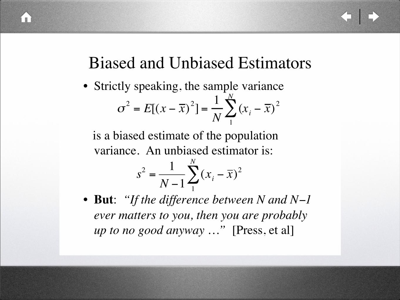
Biased and Unbiased Estimators
• Strictly speaking, the sample variance
is a biased estimate of the population
variance. An unbiased estimator is:
• But: “If the difference between N and N!1
ever matters to you, then you are probably
up to no good anyway …” [Press, et al]
!
"2
= E[(x # x )2] =
1
N(x
i# x )
2
1
N
$
!
s2
=1
N "1(x
i" x )
2
1
N
#
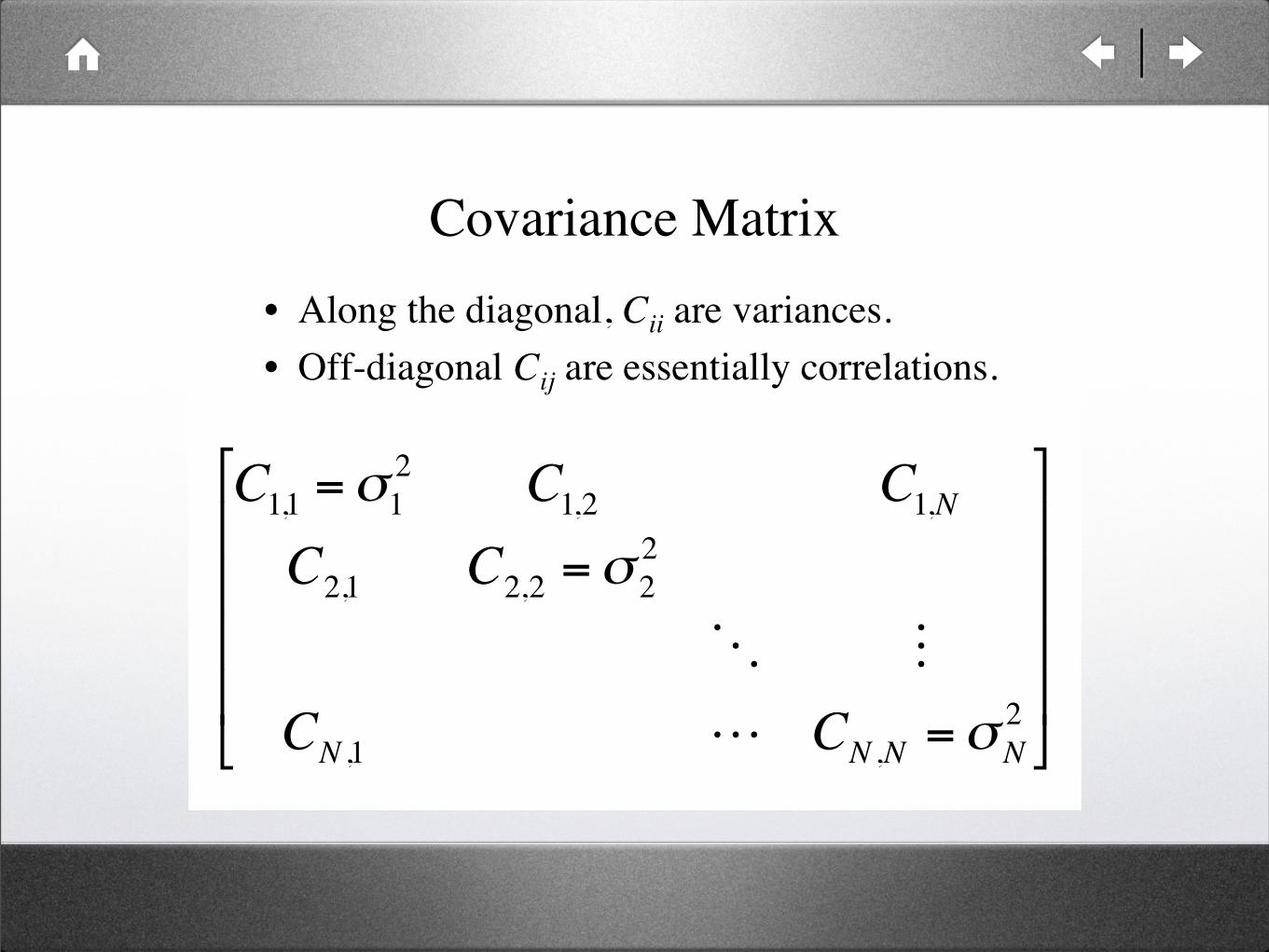
Covariance Matrix
• Along the diagonal, Cii are variances.
• Off-diagonal Cij are essentially correlations.
!
C1,1
="1
2C1,2
C1,N
C2,1
C2,2
="2
2
O M
CN ,1
L CN ,N
="N
2
#
$
% % % %
&
'
( ( ( (
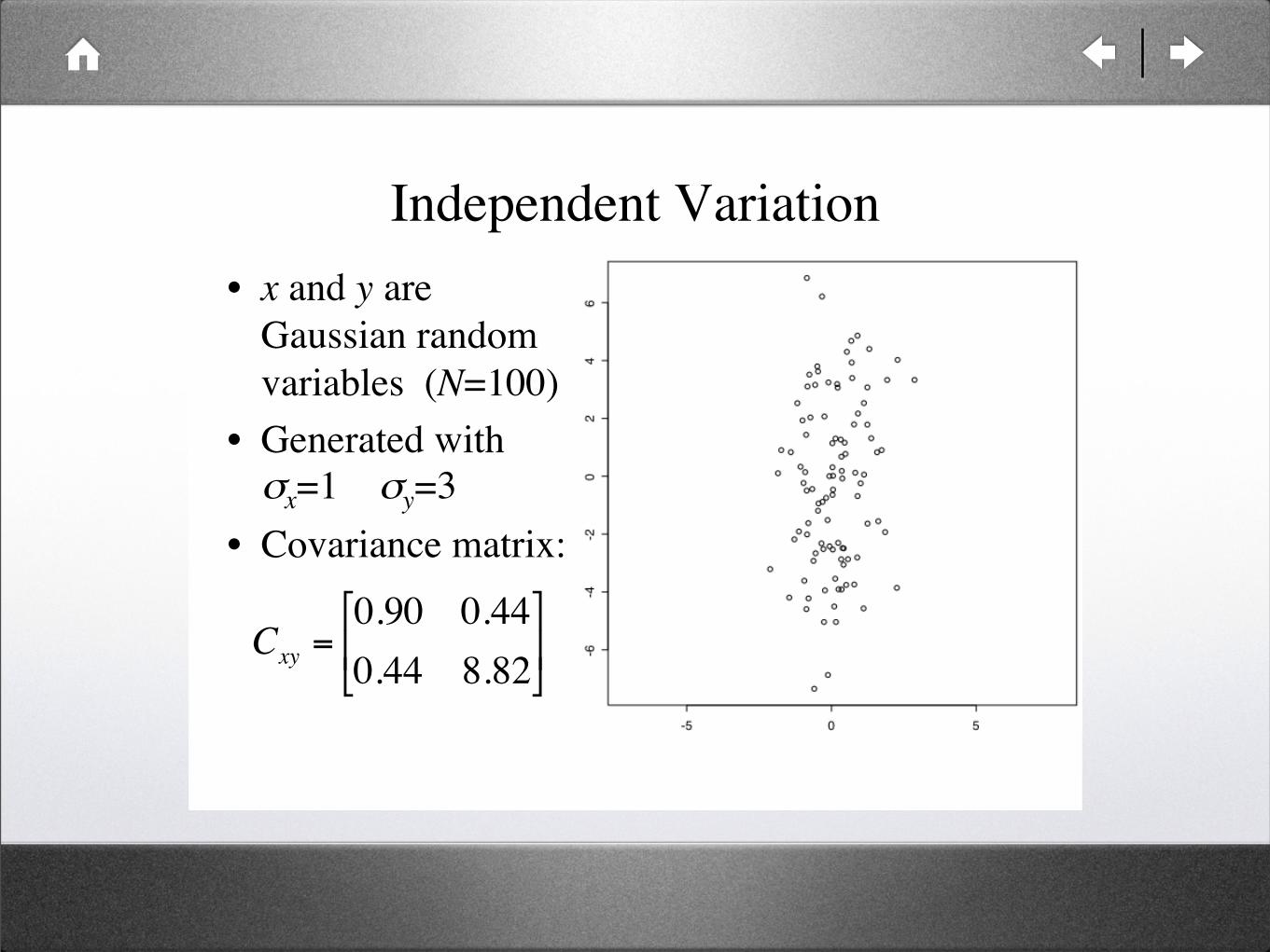
Independent Variation
• x and y are
Gaussian random
variables (N=100)
• Generated with
!x=1 !y=3
• Covariance matrix:
!
Cxy =0.90 0.44
0.44 8.82
"
# $
%
& '
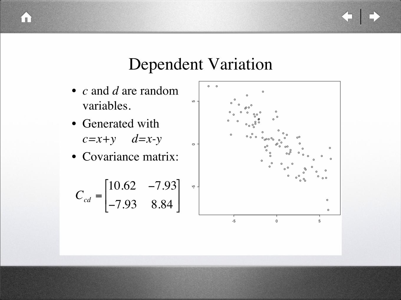
Dependent Variation
• c and d are random
variables.
• Generated with
c=x+y d=x-y
• Covariance matrix:
!
Ccd
=10.62 "7.93
"7.93 8.84
#
$ %
&
' (
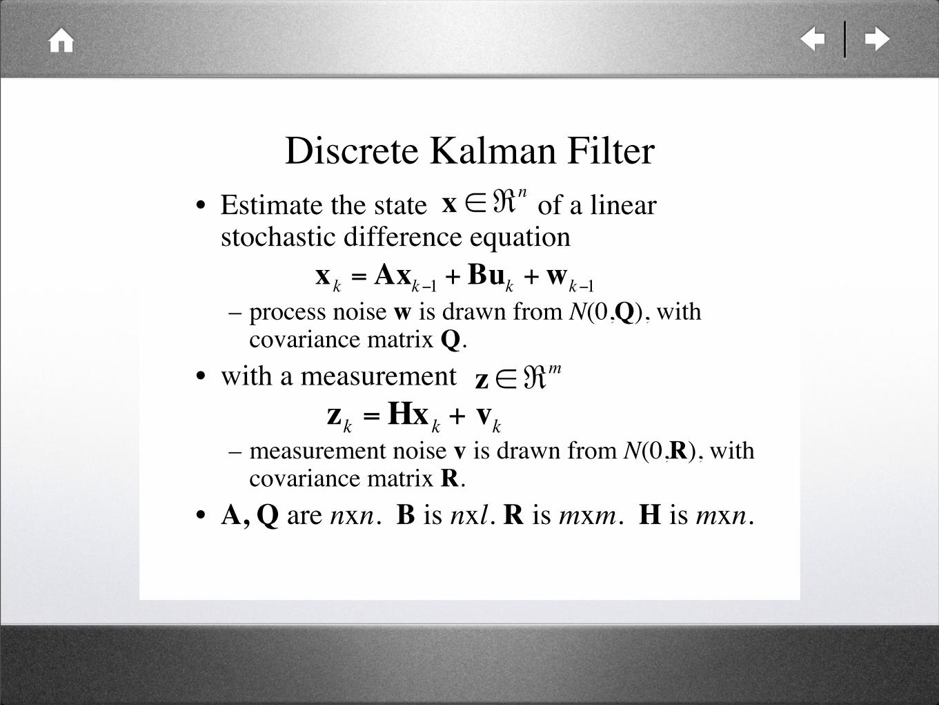
Discrete Kalman Filter
• Estimate the state of a linearstochastic difference equation
– process noise w is drawn from N(0,Q), withcovariance matrix Q.
• with a measurement
– measurement noise v is drawn from N(0,R), withcovariance matrix R.
• A, Q are nxn. B is nxl. R is mxm. H is mxn.
!
xk
=Axk"1 + Bu
k+w
k"1
!
x "#n
!
z "#m
!
zk
=Hxk+ v
k
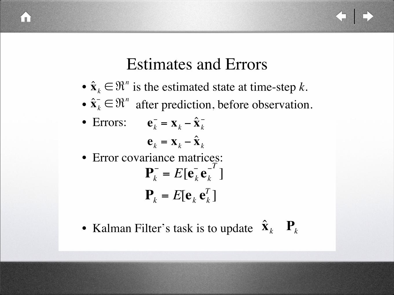
Estimates and Errors
• is the estimated state at time-step k.
• after prediction, before observation.
• Errors:
• Error covariance matrices:
• Kalman Filter’s task is to update
!
ˆ x k"#
n
!
ˆ x k
"# $
n
!
ek
" = xk" ˆ x
k
"
ek
= xk" ˆ x
k
!
Pk
"= E[e
k
"ek
"T
]
Pk
= E[ekek
T]
!
ˆ x k
Pk
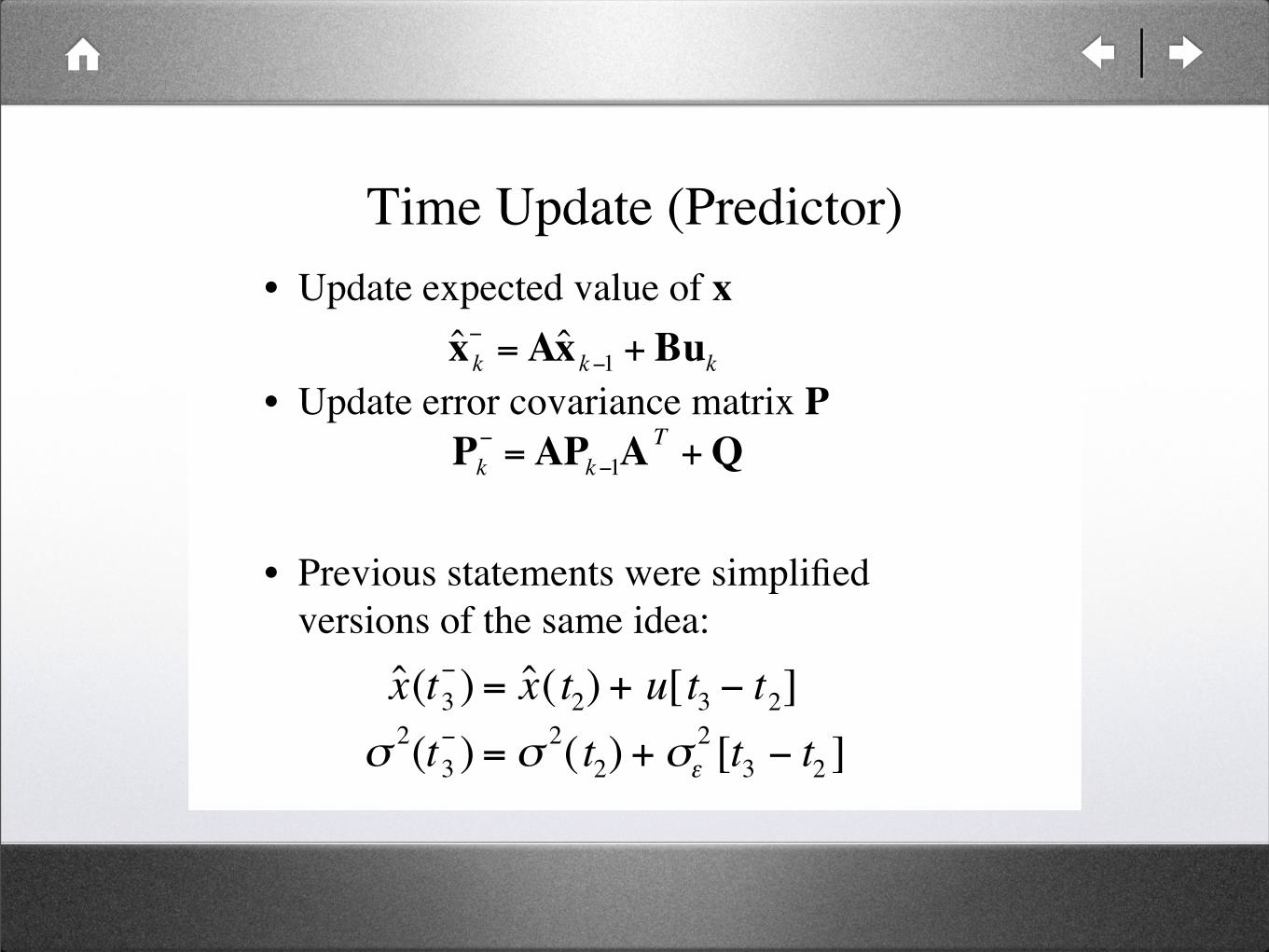
Time Update (Predictor)
• Update expected value of x
• Update error covariance matrix P
• Previous statements were simplified
versions of the same idea:
!
ˆ x k
"= Aˆ x
k"1 + Buk
!
Pk
"=AP
k"1AT
+Q
!
ˆ x (t3
") = ˆ x ( t
2) + u[ t
3" t
2]
!
"2(t3
#) = "
2( t2) + "$
2[t3# t
2]
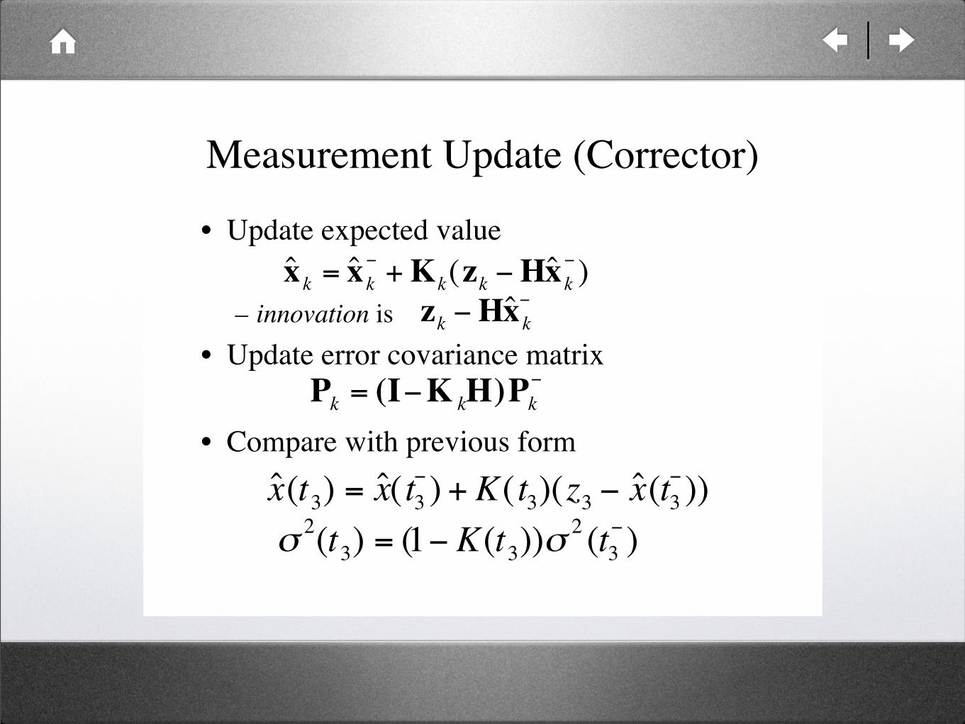
Measurement Update (Corrector)
• Update expected value
– innovation is
• Update error covariance matrix
• Compare with previous form
!
ˆ x k
= ˆ x k
"+ K
k(z
k"Hˆ x
k
")
!
zk"Hˆ x
k
"
!
Pk
= (I"KkH)P
k
"
!
ˆ x (t3) = ˆ x ( t
3
") + K( t
3)(z
3" ˆ x (t
3
"))
!
"2(t3) = (1# K(t
3))"
2(t3
#)
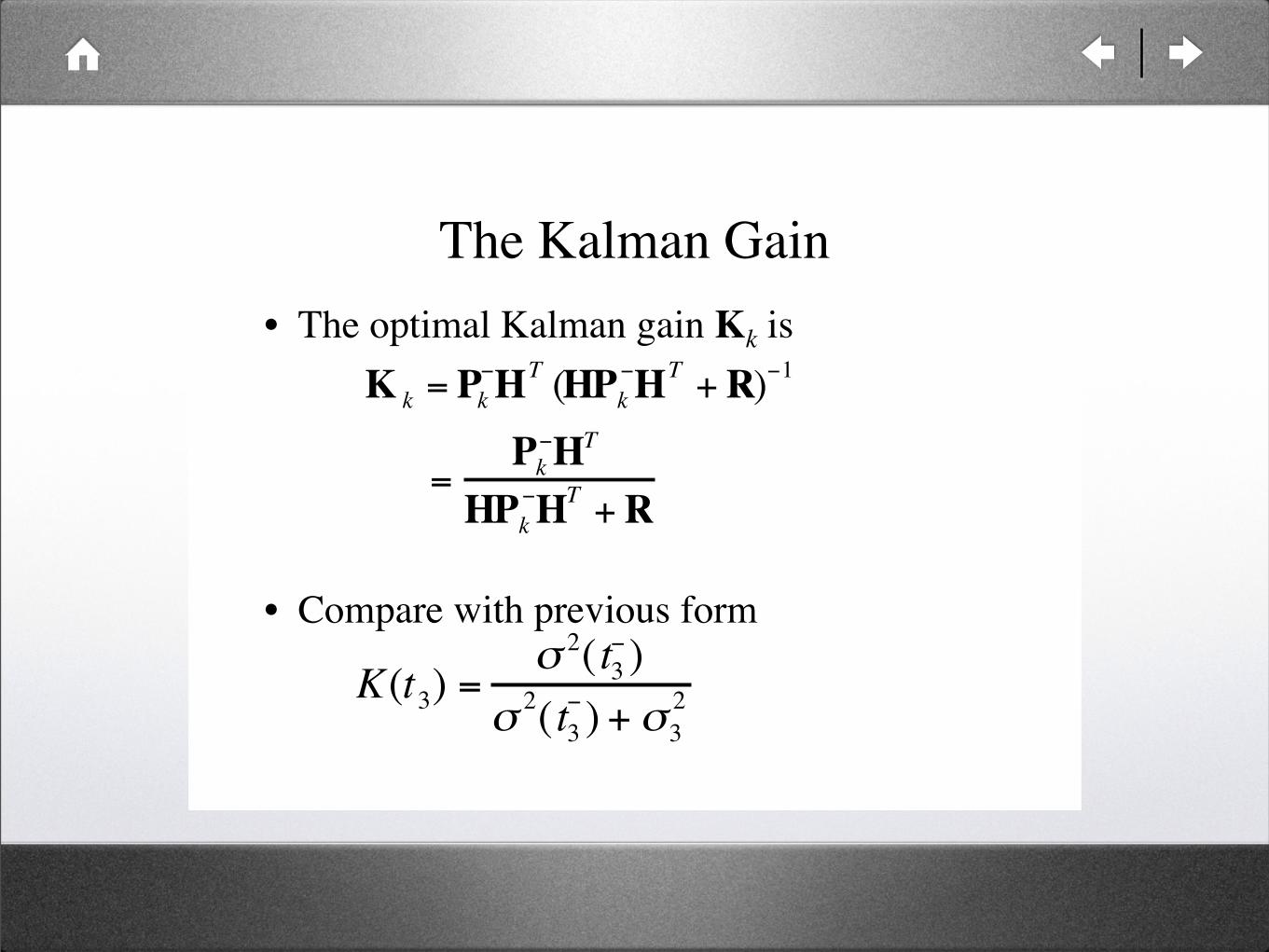
The Kalman Gain
• The optimal Kalman gain Kk is
• Compare with previous form
!
Kk
= Pk
"H
T(HP
k
"H
T+R)
"1
!
=Pk
"H
T
HPk
"H
T+R
!
K(t3) =
" 2( t3
#)
"2( t3
#) + "
3
2
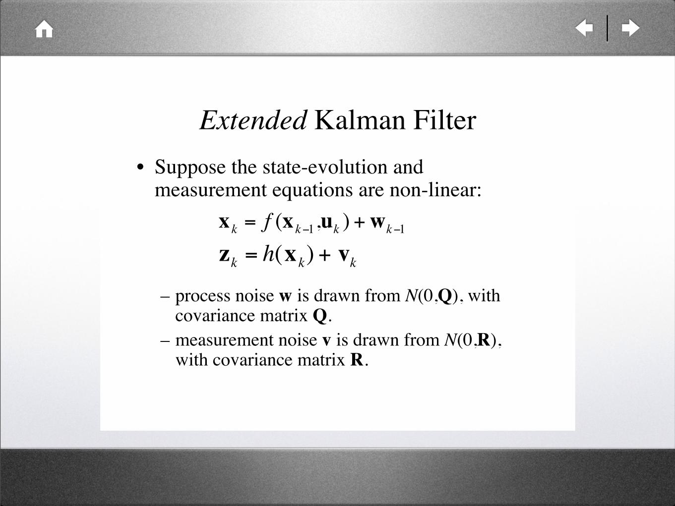
Extended Kalman Filter
• Suppose the state-evolution andmeasurement equations are non-linear:
– process noise w is drawn from N(0,Q), withcovariance matrix Q.
– measurement noise v is drawn from N(0,R),with covariance matrix R.
!
x k = f (x k"1,uk ) +wk"1
!
zk
= h(xk) + v
k
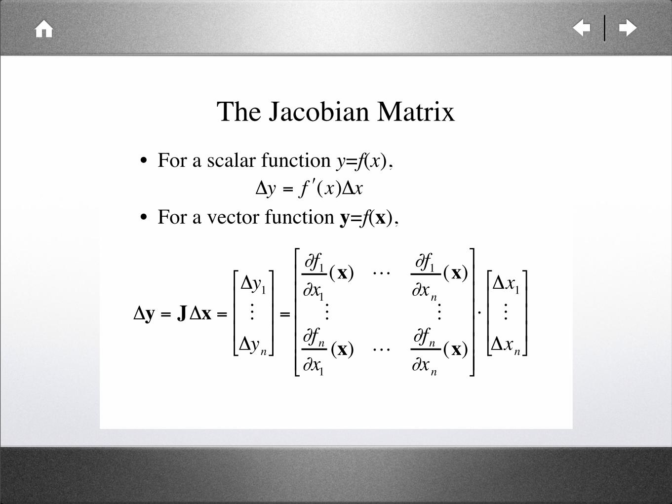
The Jacobian Matrix
• For a scalar function y=f(x),
• For a vector function y=f(x),
!
"y = # f (x)"x
!
"y = J"x =
"y1
M
"yn
#
$
% % %
&
'
( ( (
=
)f1
)x1
(x) L)f1
)xn(x)
M M
)fn)x1
(x) L)fn)xn
(x)
#
$
% % % % % %
&
'
( ( ( ( ( (
*
"x1
M
"xn
#
$
% % %
&
'
( ( (
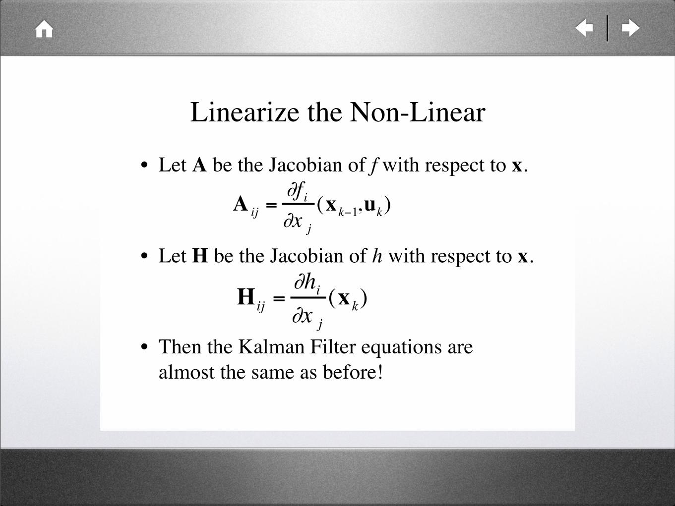
Linearize the Non-Linear
• Let A be the Jacobian of f with respect to x.
• Let H be the Jacobian of h with respect to x.
• Then the Kalman Filter equations are
almost the same as before!
!
A ij ="f i
"x j
(x k#1,uk)
!
H ij ="hi
"x j
(x k)
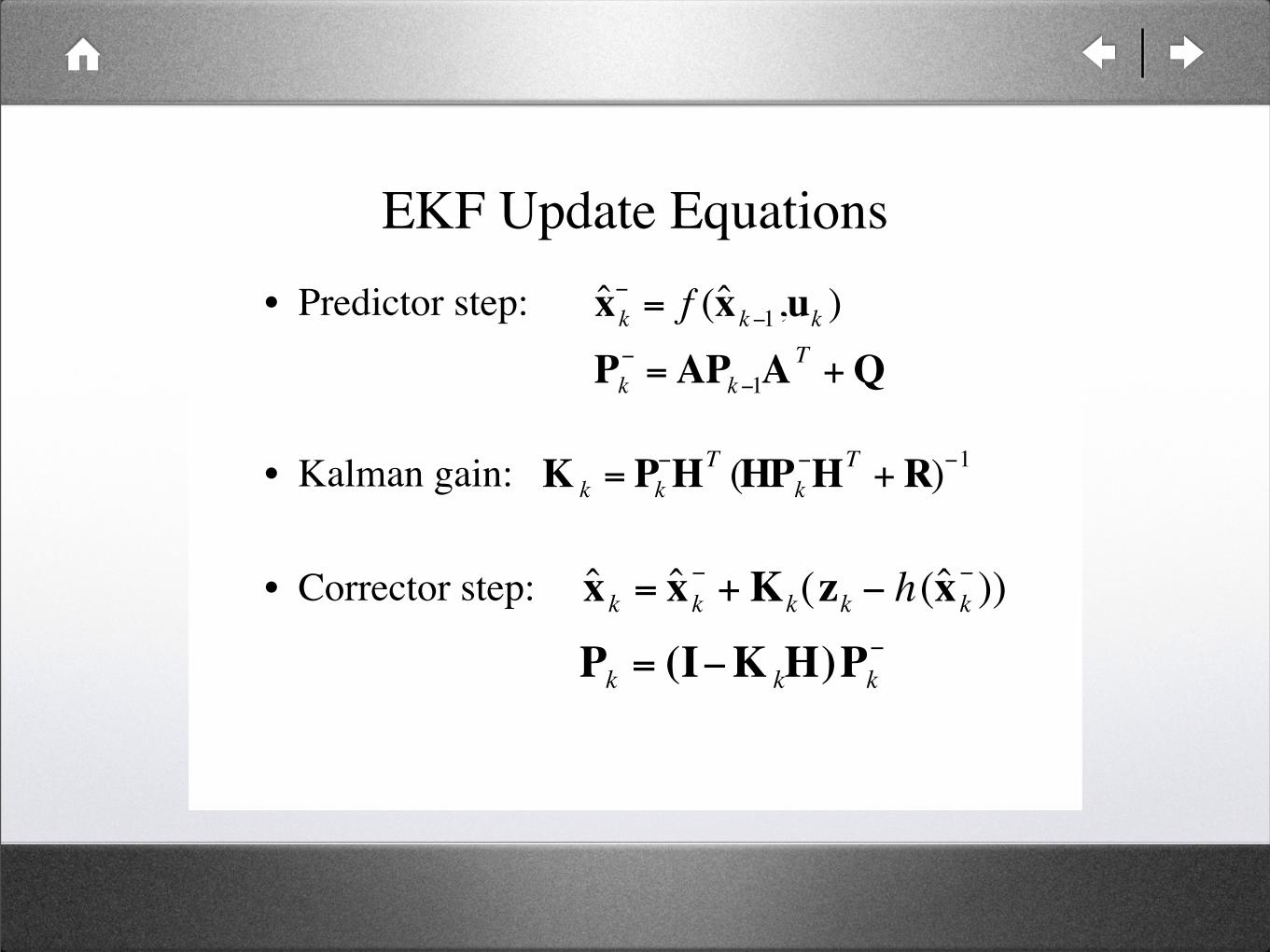
EKF Update Equations
• Predictor step:
• Kalman gain:
• Corrector step:
!
ˆ x k"
= f (ˆ x k"1,uk )
!
Pk
"=AP
k"1AT
+Q
!
Kk
= Pk
"H
T(HP
k
"H
T+R)
"1
!
ˆ x k
= ˆ x k
"+ K
k(z
k" h(ˆ x
k
"))
!
Pk
= (I"KkH)P
k
"
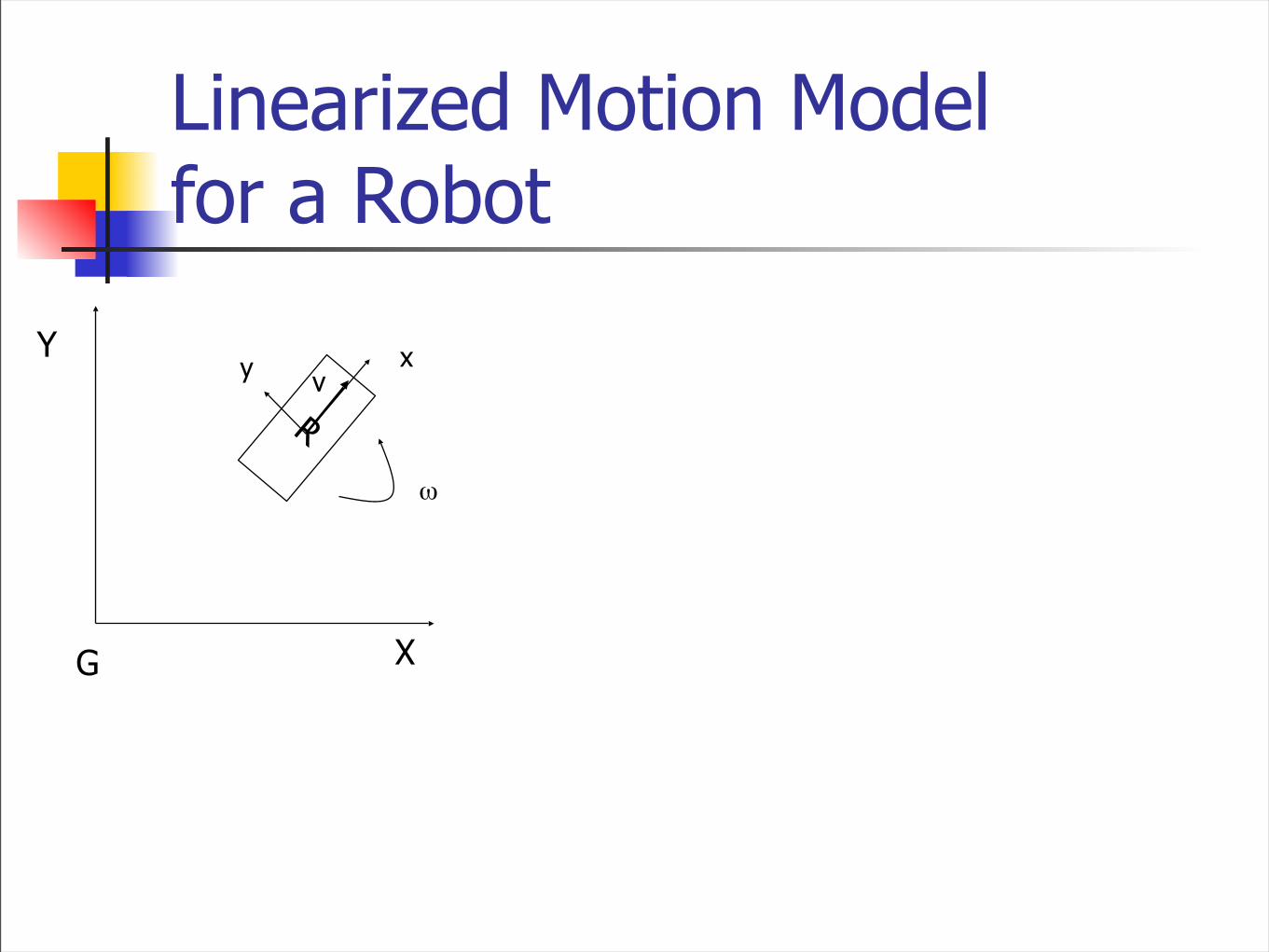
Linearized Motion Model for a Robot
R
X
Y
ω
xy
G
v
Linearized Motion Model for a Robot
R
X
Y
ω
xy
G
v
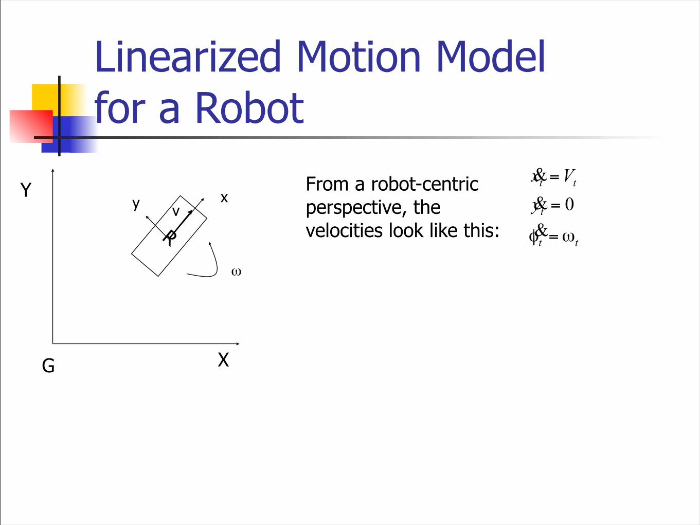
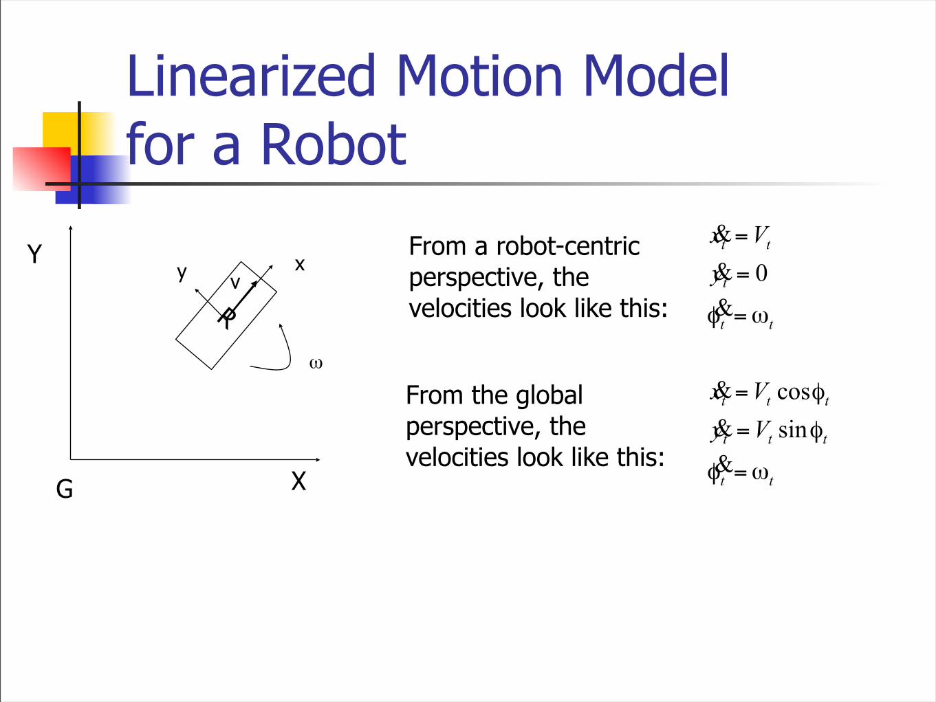
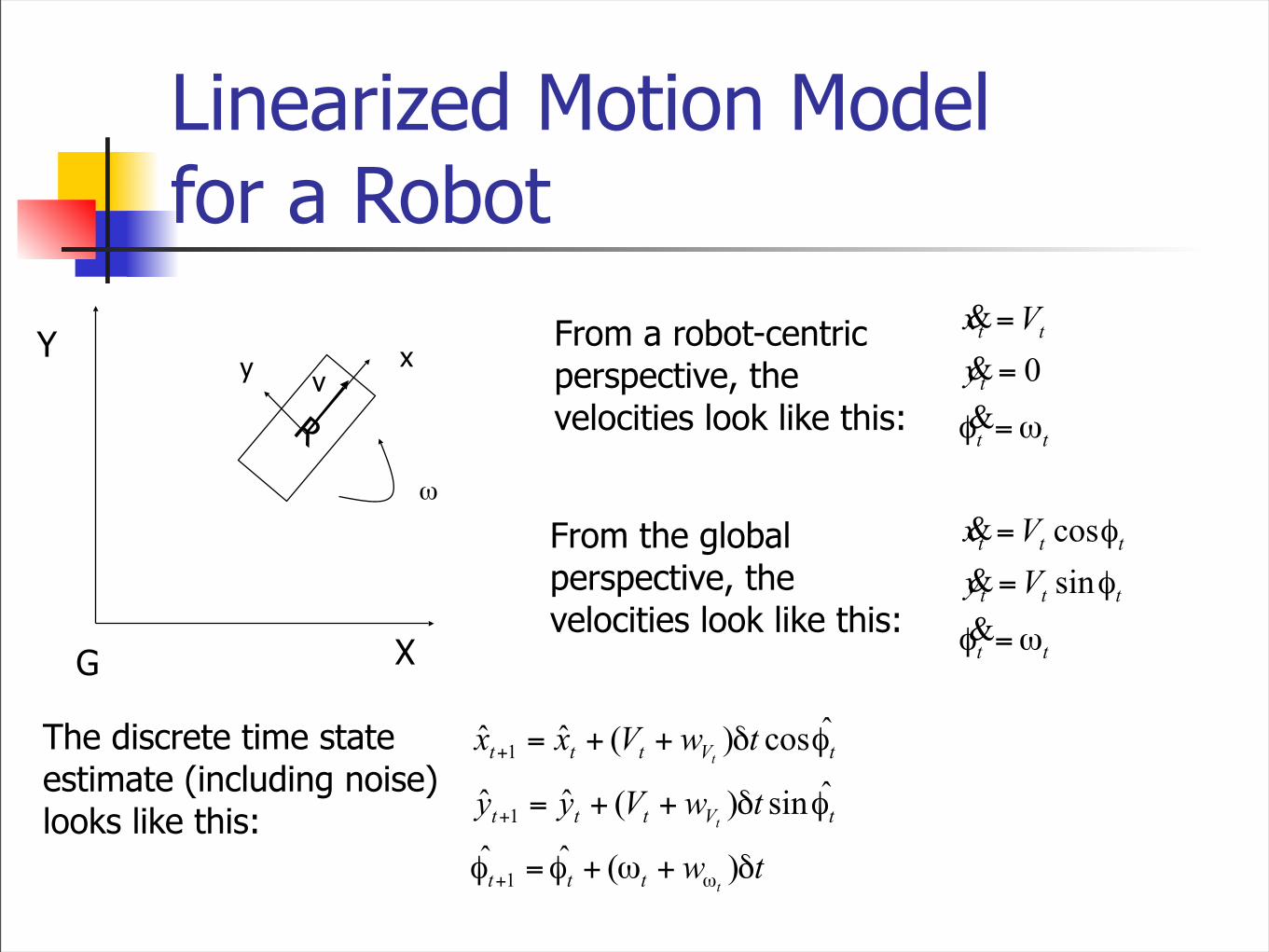
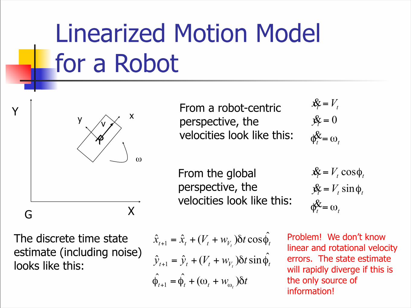
From a robot-centric perspective, the velocities look like this:
Linearized Motion Model for a Robot
R
X
Y
ω
xy
G
v
From a robot-centric perspective, the velocities look like this:
From the global perspective, the velocities look like this:
Linearized Motion Model for a Robot
R
X
Y
ω
xy
G
v
From a robot-centric perspective, the velocities look like this:
From the global perspective, the velocities look like this:
The discrete time state estimate (including noise) looks like this:
Linearized Motion Model for a Robot
R
X
Y
ω
xy
G
v
From a robot-centric perspective, the velocities look like this:
From the global perspective, the velocities look like this:
The discrete time state estimate (including noise) looks like this:
Problem! We don’t know linear and rotational velocity errors. The state estimate will rapidly diverge if this is the only source of information!
Linearized Motion Model for a RobotNow, we have to compute the covariance matrix propagationequations.
Linearized Motion Model for a Robot
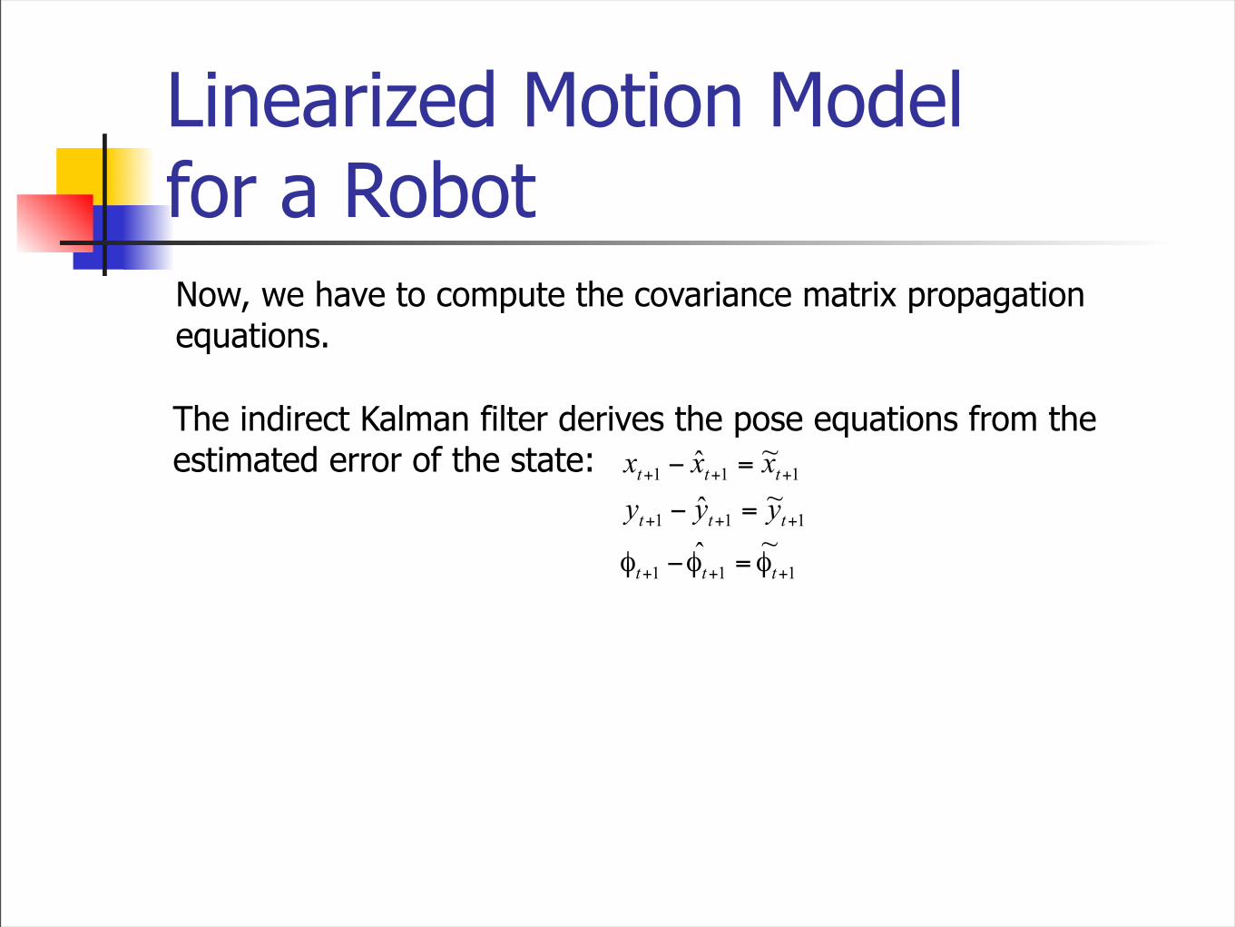
The indirect Kalman filter derives the pose equations from theestimated error of the state:
Now, we have to compute the covariance matrix propagationequations.
Linearized Motion Model for a Robot
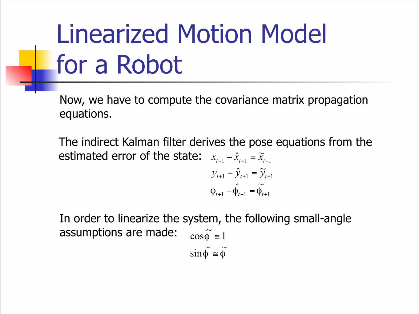
The indirect Kalman filter derives the pose equations from theestimated error of the state:
In order to linearize the system, the following small-angle assumptions are made:
Now, we have to compute the covariance matrix propagationequations.
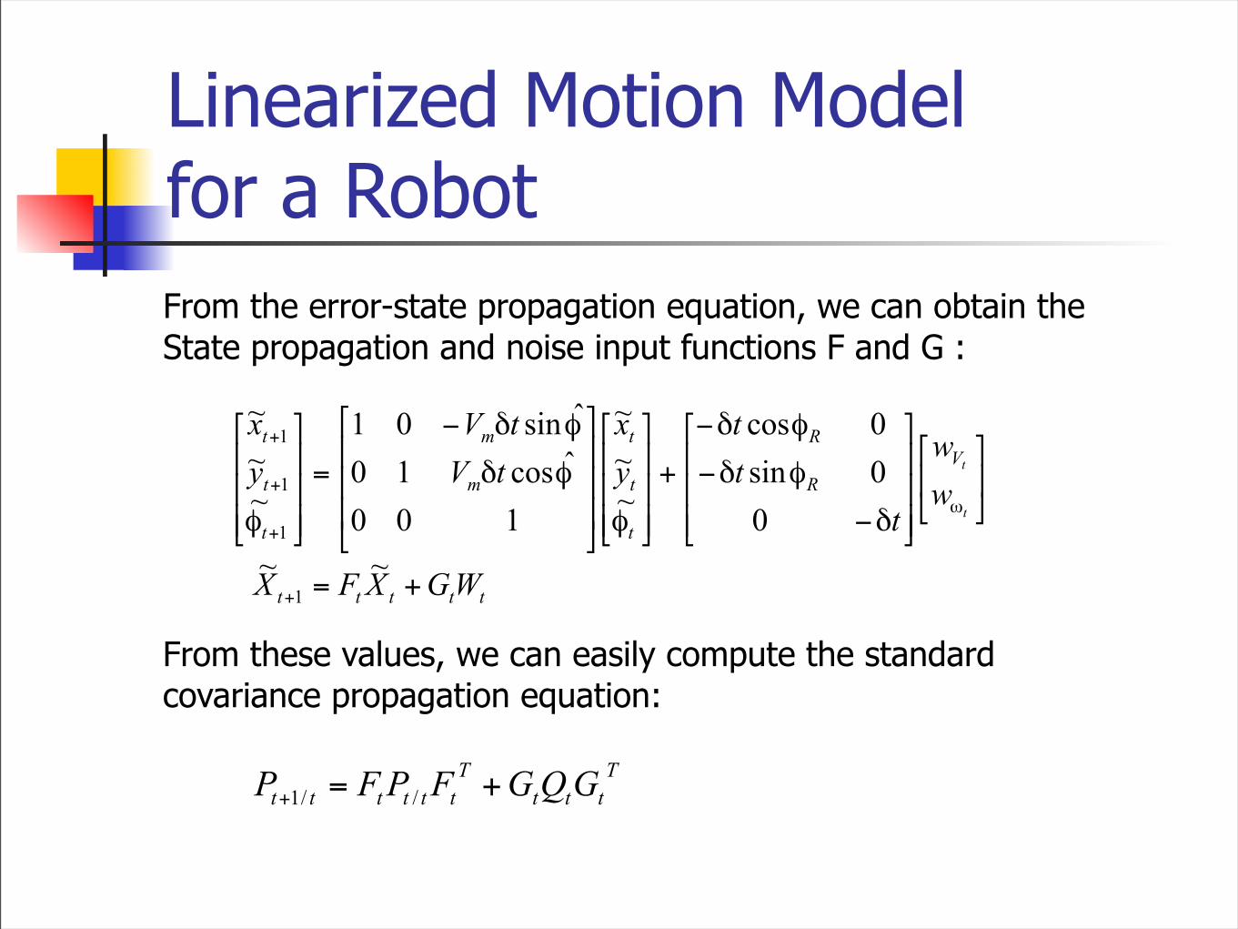
Linearized Motion Model for a RobotFrom the error-state propagation equation, we can obtain theState propagation and noise input functions F and G :
From these values, we can easily compute the standard covariance propagation equation:
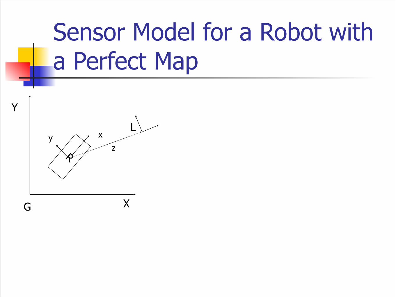
Sensor Model for a Robot with a Perfect Map
R
X
Y
xy
G
L
z
Sensor Model for a Robot with a Perfect Map
R
X
Y
xy
G
L
z
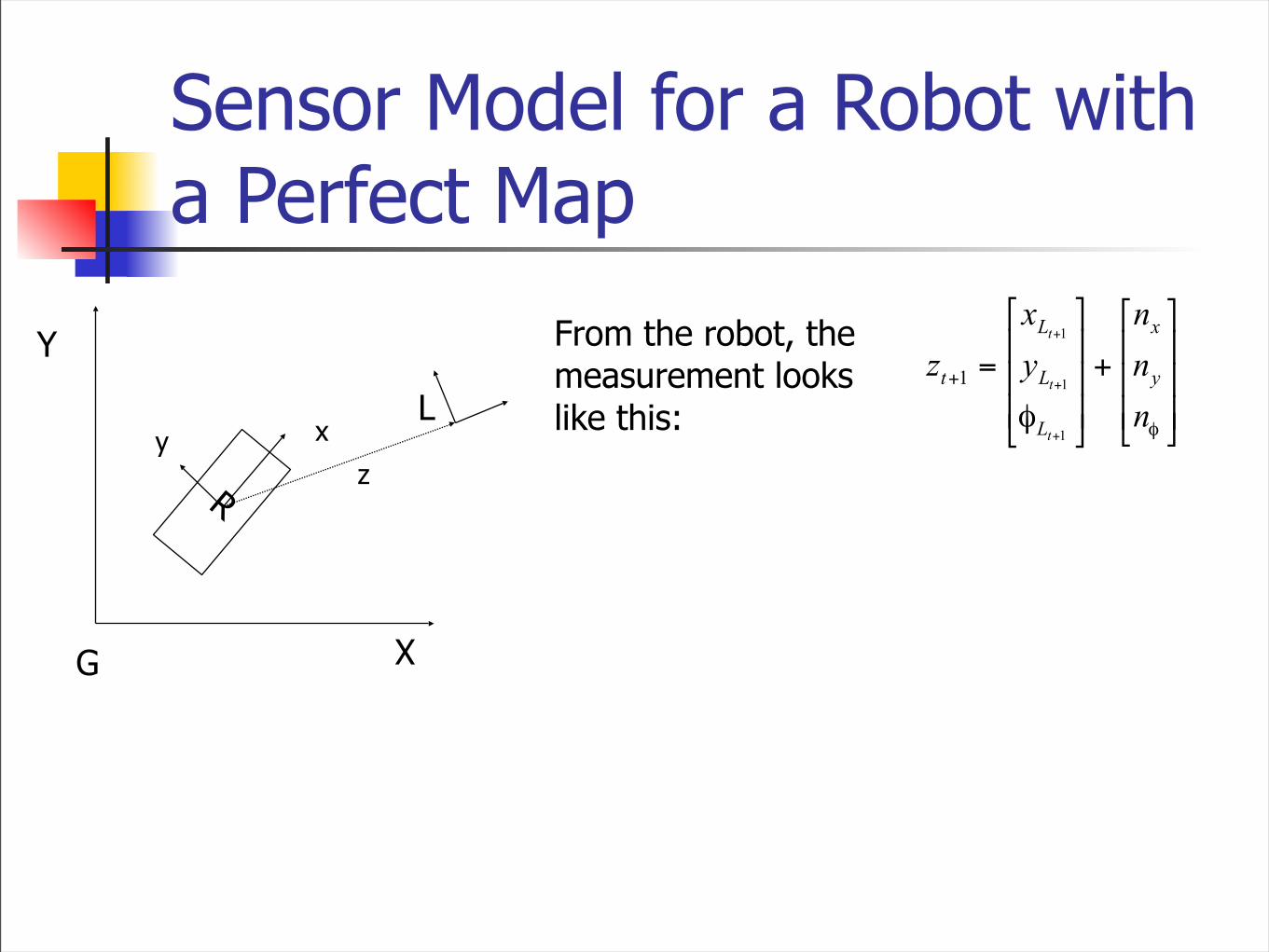
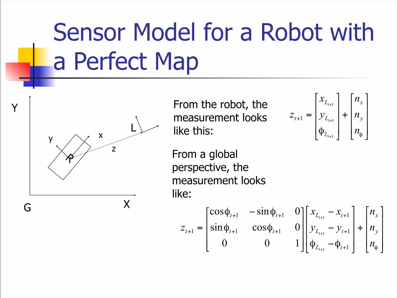
From the robot, the measurement looks like this:
Sensor Model for a Robot with a Perfect Map
R
X
Y
xy
G
L
z
From the robot, the measurement looks like this:
From a global perspective, the measurement looks like:
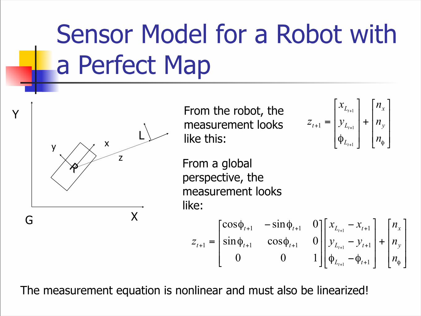
Sensor Model for a Robot with a Perfect Map
R
X
Y
xy
G
L
z
From the robot, the measurement looks like this:
From a global perspective, the measurement looks like:
The measurement equation is nonlinear and must also be linearized!
Sensor Model for a Robot with a Perfect MapNow, we have to compute the linearized sensor function. Onceagain, we make use of the indirect Kalman filter where the error in the reading must be estimated.
Sensor Model for a Robot with a Perfect MapNow, we have to compute the linearized sensor function. Onceagain, we make use of the indirect Kalman filter where the error in the reading must be estimated.
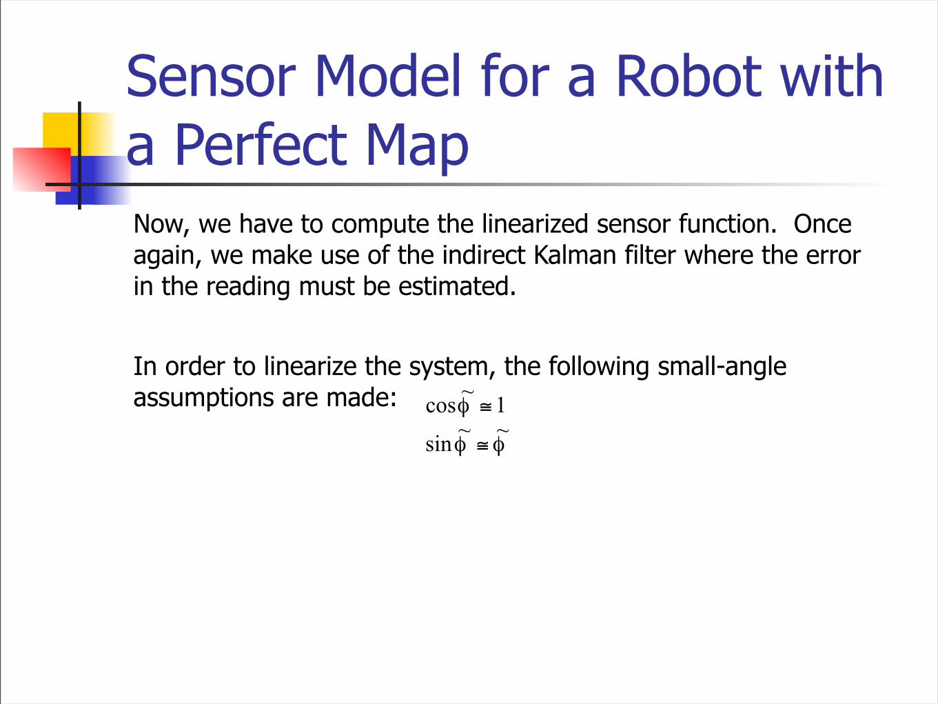
In order to linearize the system, the following small-angle assumptions are made:
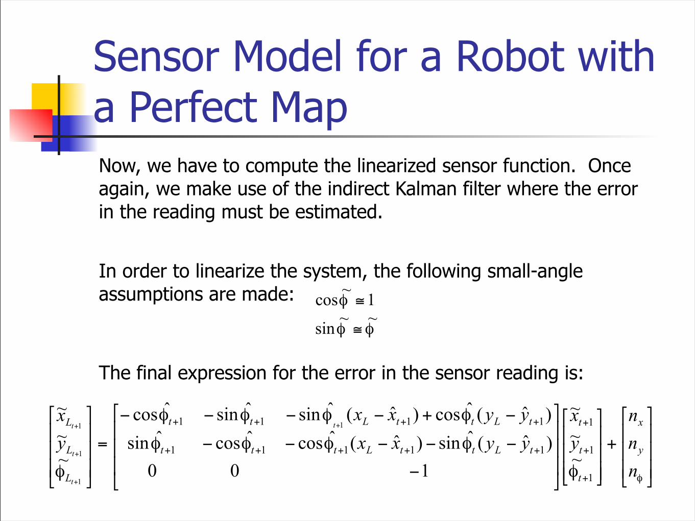
Sensor Model for a Robot with a Perfect MapNow, we have to compute the linearized sensor function. Onceagain, we make use of the indirect Kalman filter where the error in the reading must be estimated.
In order to linearize the system, the following small-angle assumptions are made:
The final expression for the error in the sensor reading is:
Slides
• Slides were taken from:
• http://www.cs.utexas.edu/~pstone/Courses/395Tfall05/resources/
• www.cs.cmu.edu/~robosoccer/cmrobobits/lectures/Kalman.ppt


