Kalman Filter(Ch. 15)

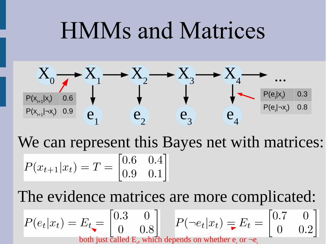
HMMs and Matrices

We can represent this Bayes net with matrices:

The evidence matrices are more complicated:

X0

X1

X2

X3

X4

e1

e2

e3

e4

...P(x

t+1|x

t) 0.6

P(xt+1

|¬xt) 0.9

P(et|x

t) 0.3

P(et|¬x

t) 0.8

both just called Et, which depends on whether e

t or ¬e

t

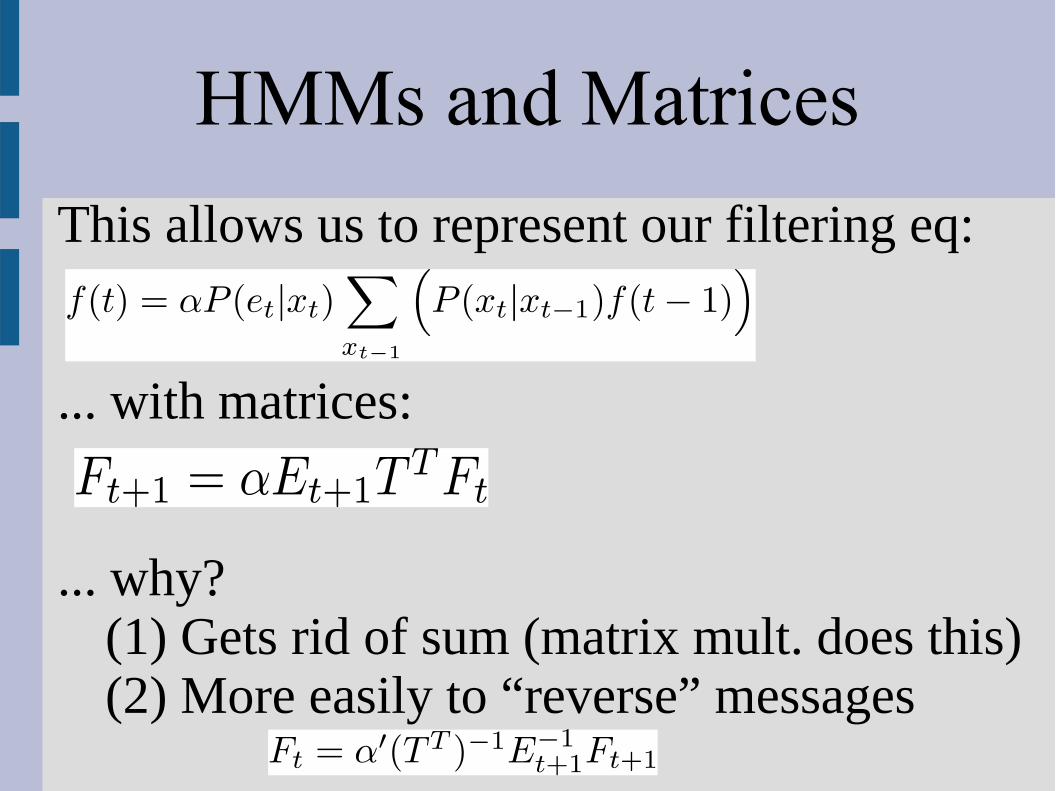
HMMs and Matrices

This allows us to represent our filtering eq:

... with matrices:

... why?(1) Gets rid of sum (matrix mult. does this)(2) More easily to “reverse” messages

HMMs and Matrices

This actually gives rise to a smoothing alg.with constant memory (we did with linear):

Smooth (constant mem):-1. Compute filtering from 1 to t-2. Loop: i=t to 1-2.1. Smooth X

i (have f(i) and backwards(i))

-2.2. Compute backwards(i-1) in normal way-2.3. Compute f(i-1) using previous slide

HMMs and Matrices

Smoothing actually has issues with “online”algorithms, where you need results mid-alg.

The stock market is an example as you havehistorical info and need choose trades today

But tomorrow we willhave the info for todayas well... need alg to not compute “from scratch”

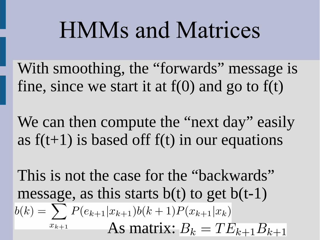
HMMs and Matrices

With smoothing, the “forwards” message isfine, since we start it at f(0) and go to f(t)

We can then compute the “next day” easilyas f(t+1) is based off f(t) in our equations

This is not the case for the “backwards”message, as this starts b(t) to get b(t-1)

As matrix:

HMMs and Matrices

The naive way would be to restart the “backwards” message from scratch

I will switch to the book’s notation of B1:t

as the backward message that uses e1 to e

t

(slightly different as Bk uses e

k+1 to e

t)

Thus we would want some way to computeB

j:t+1 from B

k:t without doing it from scrath

HMMs and Matrices

So we have:

In general:

This [1,1]T matrix is in the way, so let’s store:

... then:

... or generally if j>k:

i starts large,then decreases:for(i=j-1; i>=k; i--)

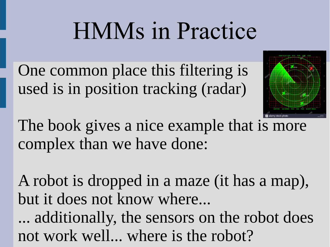
HMMs in Practice

One common place this filtering is used is in position tracking (radar)

The book gives a nice example that is morecomplex than we have done:

A robot is dropped in a maze (it has a map),but it does not know where...... additionally, the sensors on the robot doesnot work well... where is the robot?

HMMs in Practice

where walls are

HMMs in Practice

Average expected distance(Manhattan) from real

perfect sensors

20% error per direction(1-.84) = 59% at least one error

Kalman Filters

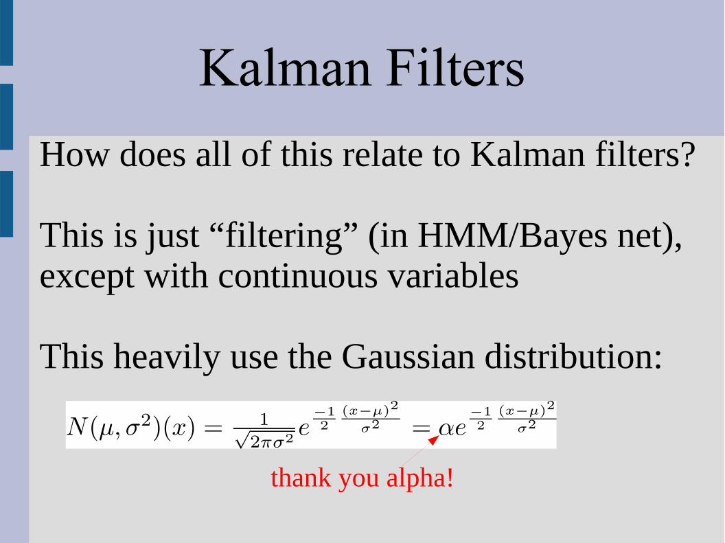
How does all of this relate to Kalman filters?

This is just “filtering” (in HMM/Bayes net),except with continuous variables

This heavily use the Gaussian distribution:

thank you alpha!

Kalman Filters

Why the preferential treatment for Gaussians?

A key benefit is that when you do our normal operations (add and multiply), if you startwith a Gaussian as input, you get Gaussian out

In fact, if you input a linear Gaussian input,you get a Gaussian out: (linear=matrix mult)

More on this later, let’s start simple

Kalman Filters

As an example, let’s say you are playingFrisbee at night

1. Can’t see exactly where friend is

2. Friend will move slightly to catch Frisbee

Kalman Filters

Unfortunately... the math is a bit ugly (asGaussians are a bit complex)

Here we assume:

How do we compute the filtering “forward”messages (in our efficient non-recursive way)?

xt

y-axis =prob x

t+1 is how much friend moves

mean

variance is “can’t see well”

Kalman Filters

Unfortunately... the math is a bit ugly (asGaussians are a bit complex)

Here we assume:

How do we compute the filtering “forward”messages (in our efficient non-recursive way)?

xt

y-axis =prob x

t+1 is how much friend moves

mean

variance is “can’t see well”erm... let’s change variable names

Kalman Filters

Unfortunately... the math is a bit ugly (asGaussians are a bit complex)

Here we assume:

How do we compute the filtering “forward”messages (in our efficient non-recursive way)?

xt

y-axis =prob x

t+1 is how much friend moves

mean

variance is “can’t see well”

Kalman Filters

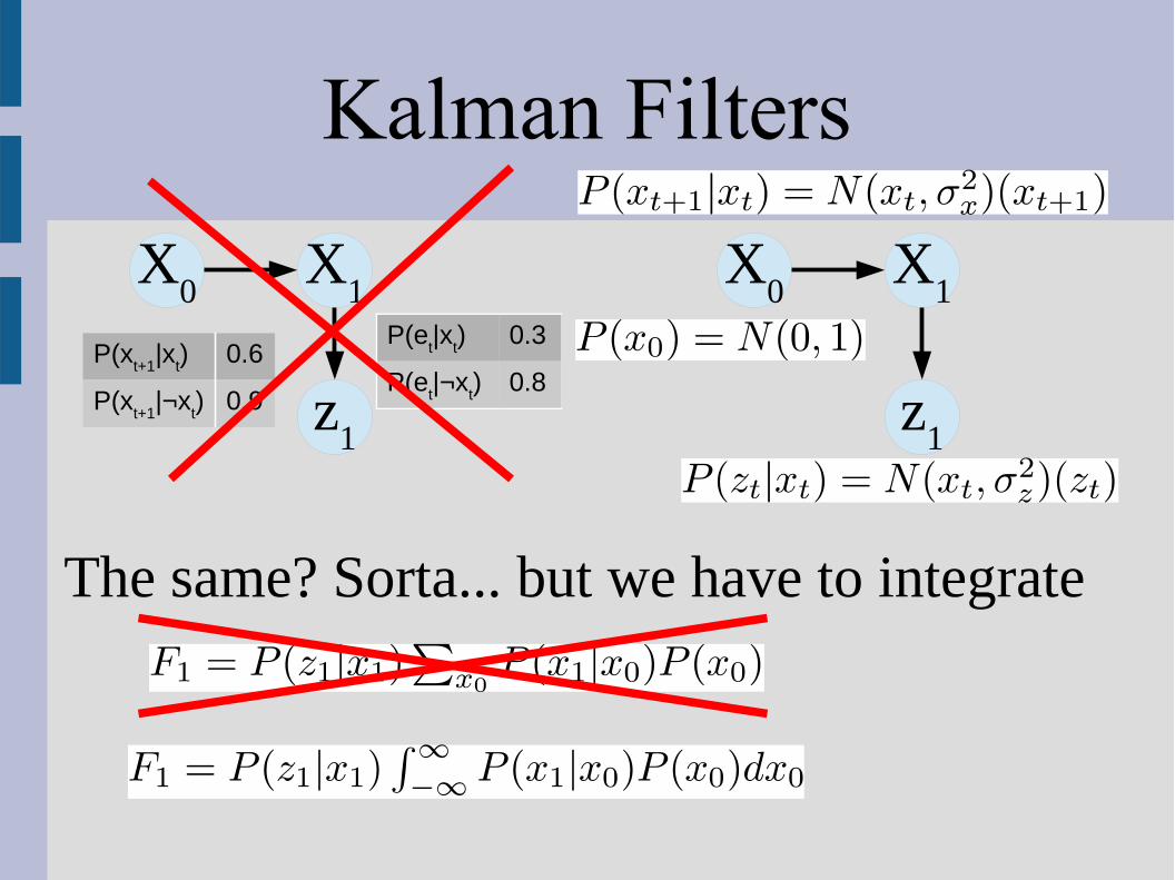
The same? Sorta... but we have to integrate

X0

X1

z1

P(xt+1

|xt) 0.6

P(xt+1

|¬xt) 0.9

P(et|x

t) 0.3

P(et|¬x

t) 0.8

X0

X1

z1

Kalman Filters

Kalman Filters

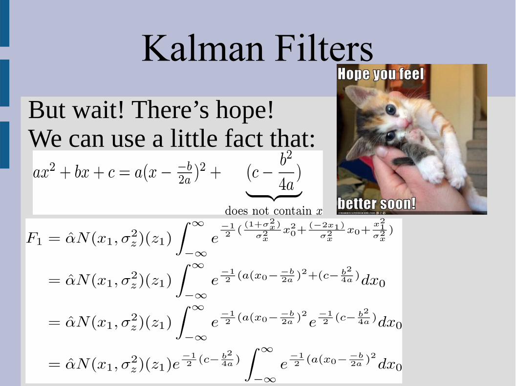
But wait! There’s hope!We can use a little fact that:

Kalman Filters

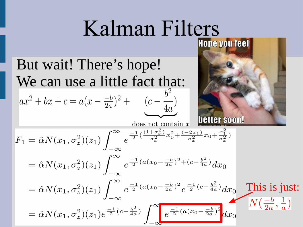
But wait! There’s hope!We can use a little fact that:

This is just:

Kalman Filters

area under all of normal distribution adds up to 1

Kalman Filters

gross after plugging ina,b,c (see book)

Kalman: Frisbee in the Dark

0

σ2=1Initially your friend is N(0,1)

0

σ2=1Initially your friend is N(0,1)

Throw not perfect, so friendhas to move N(0,1.5)

σ2=1.5

(i.e. move from black to red)

Kalman: Frisbee in the Dark

0

σ2=1But you can’t actually see your friend too clearly in the dark

You thought you saw them at 0.75 (σ2=0.2)

σ2=1.5

Kalman: Frisbee in the Dark

0

σ2=1Where is your friend actually?σ2=1.5

σ2=0.2

0.75

Kalman: Frisbee in the Dark

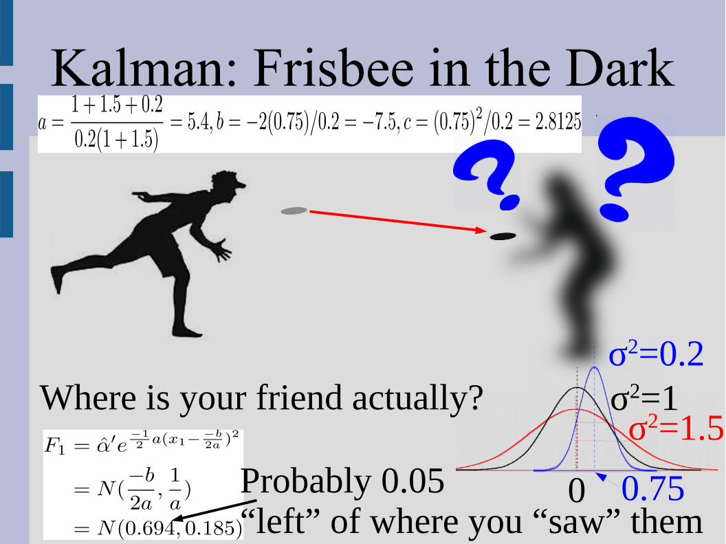
0

σ2=1Where is your friend actually?σ2=1.5

σ2=0.2

0.75Probably 0.05“left” of where you “saw” them

Kalman: Frisbee in the Dark

Kalman Filters

So the filtered “forward” message for throw 1 is:

To find the filtered “forward” message forthrow 2, use instead of(this does change the equations as you needto involve a μ for the old )

The book gives you the full messy equations:

Kalman Filters

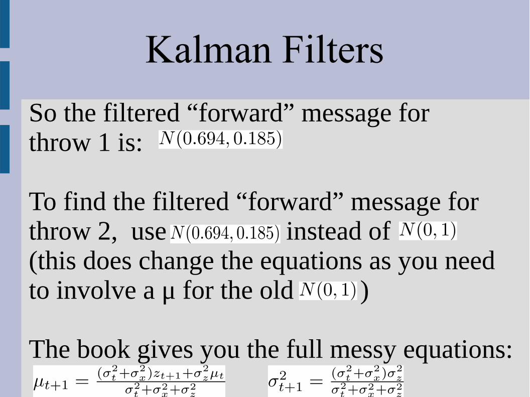
So the filtered “forward” message for throw 1 is:

To find the filtered “forward” message forthrow 2, use instead of(this does change the equations as you needto involve a μ for the old )

The book gives you the full messy equations:

Kalman Filters

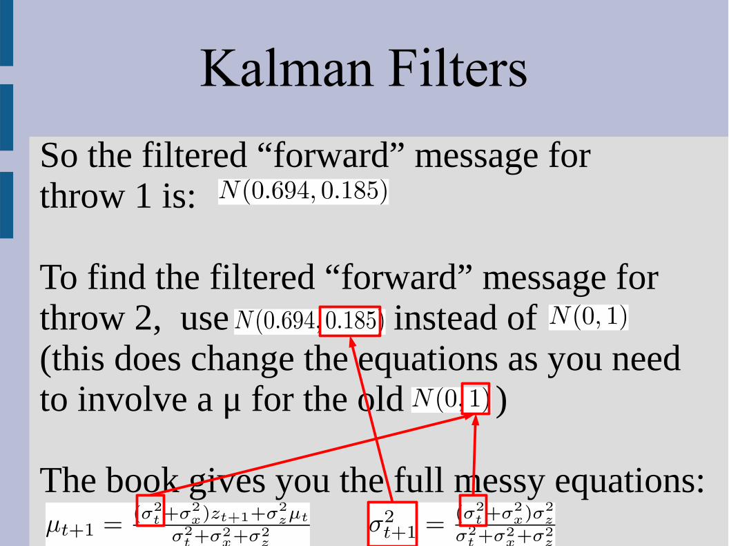
So the filtered “forward” message for throw 1 is:

To find the filtered “forward” message forthrow 2, use instead of(this does change the equations as you needto involve a μ for the old )

The book gives you the full messy equations:

Kalman Filters

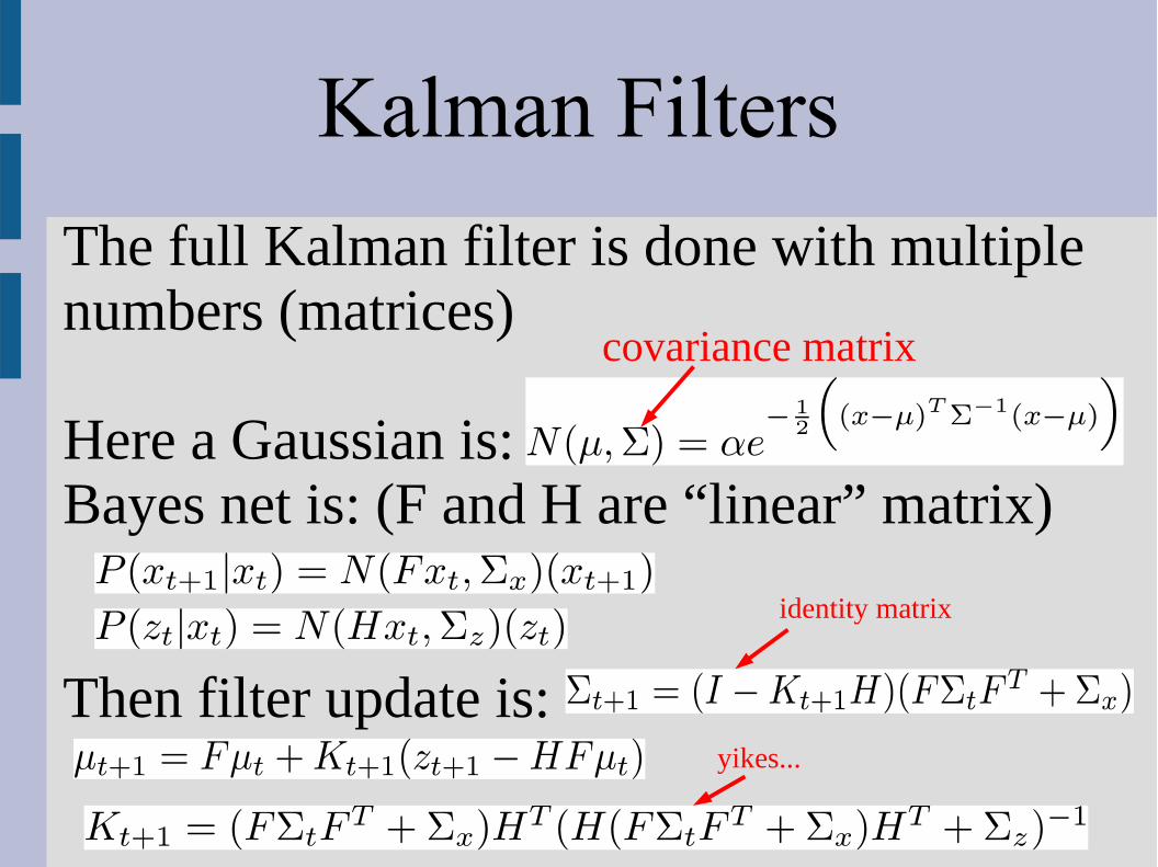
The full Kalman filter is done with multiplenumbers (matrices)

Here a Gaussian is:Bayes net is: (F and H are “linear” matrix)

Then filter update is:

covariance matrix

identity matrix

yikes...

Kalman Filters

Often we use for a 1-dimensionalproblem with both position and velocity

To update xt+1

, we would want:

In matrix form:

so:

So our “mean” at t+1 is [our position at x+vx]

Kalman Filters

Here’s a Pokemon example (not technical)https://www.youtube.com/watch?v=bm3cwEP2nUo

Kalman Filters

Downsides?

In order to get “simple” equations, we are limited to the linear Gaussian assumption

However, there are some cases when thisassumption does not work very well at all

Kalman Filters

Consider the example of balancing a pencilon your finger

How far to the left/right will the pencil fall?

Below is not a good representation:

Kalman Filters

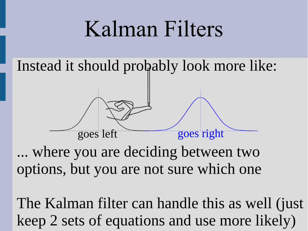
Instead it should probably look more like:

... where you are deciding between twooptions, but you are not sure which one

The Kalman filter can handle this as well (just keep 2 sets of equations and use more likely)

goes left goes right

Kalman Filters

Unfortunately if you repeat this “pencil balance” on the new spot... you would need4 sets of equations

3rd attempt: 8 equations4th attempt: 16 equations... this exponential amount of work/memorycannot be done for a large HMM