THE SADDLE POINT METHOD AND ITS APPLICATIONS TO NUMBER THEORY Kannappan Sampath A thesis submitted in partial fulfillment of the requirements for the degree of Master of Science in Mathematics and Statistics Department of Mathematics and Statistics Queen’s University August, 2015 Copyright c ⃝ Kannappan Sampath, 2015
Transcript
THE SADDLE POINT METHODAND ITS APPLICATIONS TO
NUMBER THEORY
Kannappan Sampath
A thesis submitted in partial fulfillment of therequirements for the degree of Master of Science in
Mathematics and Statistics
Department of Mathematics and StatisticsQueen’s University
August, 2015
Copyright c⃝ Kannappan Sampath, 2015
Abstract
In this thesis, we study the classical procedures useful in obtainingasymptotic expansions of functions defined by integrals and their ap-plications to number theory. The final chapter in the thesis reports ona recent joint work with Ram Murty on the theme of using arithmeticformulas to obtain asymptotic formulas to study the Fourier coefficientsof the j-function and a related sequence jmm⩾0 of modular functions.
3
Acknowledgements
First and foremost, I would like to thank my family for their un-conditional support.
I would like to thank my advisor Professor Ram Murty for intro-ducing me to the ideas discussed in this report. I also thank him forreading through the drafts of this report and providing me with cor-rections and suggestions. I am grateful to Professor Jamie Mingo andProfessor Ivan Dimitrov for agreeing to serve on my examination com-mittee. I also thank them for their careful reading of this report andfor giving me corrections and suggestions. Needless to say, any errorthat remains is solely mine.
I would like to thank my friends Henry de Valence, Dinushi Munas-inghe, Siddhi Pathak, Francois Seguin, Akshaa Vatwani and Peng-JieWong for being there to talk Mathematics with and for getting meaccustomed to the ways of life here at Kingston.
Last but not least, my hearty thanks are also due to SiobhainBroekhoeven for being an overall wonderful host.
5
Contents
Abstract 3
Acknowledgements 5
Introduction 9
Chapter 1. Asymptotics: An introduction 111. Introduction 112. Asymptotic Expansions 123. Integration by parts 154. A very simple proof of Stirling’s formula for n! 16
Chapter 2. Asymptotic methods for integrals depending on alarge parameter 21
1. Watson’s Lemma 212. Laplace’s Method 253. The Method of Steepest Descent 29
Chapter 3. Two Examples 351. Stirling’s formula for the complex Gamma function 352. The Mellin transform and its application to asymptotics 36
Chapter 4. On the asymptotic formula for the Fourier coefficientsof j-function 39
1. Preliminaries 392. Asymptotic formula for j(τ) 413. On the sequence jmm of modular functions 46
Bibliography 49
7
Introduction
Let H denote the upper half-plane z ∈ C : ℑ(z) > 0. Thej-function defined by
j(τ) =(1 + 240
∑∞n=1 σ3(n)q
n)3
q∏∞
n=1(1− qn)24, q = e2πiτ , τ ∈ H
is an SL2(Z)-invariant modular function on H whose q-expansion ati∞ is:
For definitions and basic facts about modular forms, see [22] or [18].On the one hand, the values of the j-function at imaginary quadratic ir-rationalities, called singular moduli, that have been studied extensivelysince Kronecker, generate Hilbert class fields while on the other, thecoefficients c(n) (n ⩾ −1, n = 0) in the q-expansion of j(τ) − 744 ap-pear as dimensions of the head representations of the largest sporadicfinite simple group, the Monster group. The values of the j-functionalso tell one elliptic curve defined over C from another upto isomor-phism. In what can be described as a marriage between these valuesand coefficients, Kaneko [15] discovered a closed formula for c(n) basedon Zagier’s work [25] on ‘modular’ traces of singular moduli. The ap-pearance of this function in these widely varied contexts makes it thetheoretical underpinning of many mathematical phenomena.
Using the circle method introduced by Ramanujan and Hardy [13]to study the partition function p(n), Hans Petersson [16] and laterHans Rademacher [17] independently derived the following asymptoticformula for c(n):
(1) c(n) = [qn]j ∼ e4π√n
√2n3/4
as n→ ∞.
Here we use the convenient notation [qn]f for the coefficient of qn ina q-series f . We must also note that, by using different techniques,Hans Petersson and Hans Rademacher also derived a convergent seriesexpressing the Fourier coefficients for the j-function.
9
10 INTRODUCTION
In 2005, N. Brisebarre and G. Philibert [3] revisited this classi-cal work to derive effective upper and lower bounds (as opposed tomere asymptotic formulas) more generally for the Fourier coefficientsof powers of the j-function. In their paper, using Ingham’s Tauberiantheorem [14], they indicate a quick proof of the following asymptoticformula:
(2) [qn]jm ∼ m1/4e4π√nm
√2n3/4
as n→ ∞.
In 2013, M. Dewar and Ram Murty [9] derived the asymptotic formulafor [qn]jm (and more generally, coefficients of weakly holomorphic mod-ular forms) without using the circle method. They applied an algebraicformula due to Bruinier and Ono [4].
The principal aim of this report is to present a new proof of theasymptotic formula for c(n) as n → ∞. This proof is inspired by theidea that arithmetic (and algebraic) formulas give asymptotic formulaswhen combined with variants of the saddle point method introducedby Ram Murty and Michael Dewar in their earlier works [10] and [9].Towards the goal, we begin by defining asymptotic expansions andstudying their fundamental properties in Chapter 1. In Chapter 2, westudy the classical procedures useful in deriving asymptotic expansions.Two examples are indicated in Chapter 3. In the final Chapter 4, wederive the asymptotic formula for c(n) as n→ ∞ using the arithmeticformula of Kaneko [15] and Laplace’s method.
CHAPTER 1
Asymptotics: An introduction
Those skilled in mathematical analysis know that itsobject is not simply to calculate numbers, but that itis also employed to find the relations betweenmagnitudes which cannot be expressed in numbersand between functions whose law is not capable ofalgebraic expression.
Antoine Augustin Cournot. Researches into theMathematical Principles of the Theory of Wealth,
1897, English transl. by Nathaniel T. Bacon. p. 137
1. Introduction
In many physical and mathematical problems, it is desirable tounderstand the asymptotic behaviour of functions as the independentparameter tends to a limit. These functions may arise as solutionsto differential equations, as integral transforms of functions; or per-haps arise from combinatorial considerations as generating functionsof different kinds. When confronted with problems that require suchan understanding, one’s intuition often formulates statements like “thefunction grows rapidly/slowly”, “the error incurred in this approxima-tion is small” and occassionally, more precise statements like “it growslike log x when x is large” etc. The subject of asymptotic analysis isclassically rooted in attempts to make such intuitively plausible state-ments more precise.
In this chapter, we study the notion of an asymptotic expansion.This chapter owes much to the texts of Bender and Orszag [1] andWong [24]. We take the utilitarian approach to the subject introducingno more than what is needed for our purposes. Consequently, we willonly rarely make historical remarks.
Important Conventions. We shall use the letters x, y etc. forreal variables while s, z, ω, ζ etc. for complex variables. For z ∈ C, thenotation arg(z) means the principal branch of the argument so that−π < arg(z) ⩽ π.
11
12 1. ASYMPTOTICS: AN INTRODUCTION
1.1. Bachmann-Landau Symbols. Let f and g be two complexvalued functions on Ω ⊆ C. Recall the following notation (here z0 ∈ Ωor z0 = ∞):
f(z) = O(g(z)) as z → z0: this means there exists a constant K suchthat |f(z)| < K|g(z)| for all z ∈ U ∩ Ω where U is an openneighbourhood of z0.
f(z) = o(g(z)) as z → z0: this means that limz→z0 f(z)/g(z) = 0.
Remark 1.1. When we work with a fixed subset Ω of C, the limitsin asymptotic statements are assumed to be taken along paths in Ω.For example, if Ω = N, the statement that ω → ∞ just means thatω → +∞.
We write that f(z) ∼ g(z) as z → z0 if limz→z0 f(z)/g(z) = 1.
1.2. Asymptotic relations over R versus C. Given a functionf , one of the principal reasons to study the function g for which the as-ymptotic relation f ∼ g holds is to understand its “leading behaviour”at z = z0 where z0 ∈ C or z0 = ∞. So, we would like this g to be rea-sonably simple, say a function involving the exponential function andpowers of z − z0 (resp. 1
z), and independent of the path along which
the limit z → z0 is taken. A remarkable subtlety here is that thesetwo requirements are practically incompatible if Ω contains an openball around z0. This is due to a simple phenomenon discovered by SirGeorge Stokes (1864) and is related to the exponential function. For adiscussion of this phenomenon, we recommend [1, p.115].
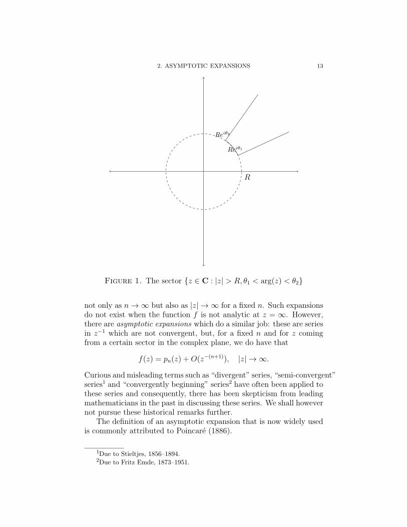
Without getting too technical at this point, we mention that thekey difficulty is that the path along which the limit z → z0 is takenmay wind itself around the point z0 a number of times. So, we shallusually ask that the limit limz→z0 f(z)/g(z) be equal to 1 when takenalong paths in a sector of the form z ∈ C : |z| > R, θ1 < arg(z) < θ2(see Figure 1).
2. Asymptotic Expansions
A function f(z) which is analytic at z = ∞ can be expanded inits Laurent series, more plainly, it is given by a power series in z−1
converging in some annulus of the form |z| > R. Recall the elementaryyet remarkable property of the partial sums pn(z) of the Laurent seriesof f(z):
(3) f(z) = pn(z) + o(1)
2. ASYMPTOTIC EXPANSIONS 13
R
Reiθ1
Reiθ2
Figure 1. The sector z ∈ C : |z| > R, θ1 < arg(z) < θ2
not only as n→ ∞ but also as |z| → ∞ for a fixed n. Such expansionsdo not exist when the function f is not analytic at z = ∞. However,there are asymptotic expansions which do a similar job: these are seriesin z−1 which are not convergent, but, for a fixed n and for z comingfrom a certain sector in the complex plane, we do have that
f(z) = pn(z) +O(z−(n+1)), |z| → ∞.
Curious and misleading terms such as “divergent” series, “semi-convergent”series1 and “convergently beginning” series2 have often been applied tothese series and consequently, there has been skepticism from leadingmathematicians in the past in discussing these series. We shall howevernot pursue these historical remarks further.
The definition of an asymptotic expansion that is now widely usedis commonly attributed to Poincare (1886).
1Due to Stieltjes, 1856–1894.2Due to Fritz Emde, 1873–1951.
14 1. ASYMPTOTICS: AN INTRODUCTION
Definition 2.1. Let f : Ω → C be functions on a domain Ω ⊆ C. Wesay that
(4)∞∑n=0
anz−n
is an asymptotic expansion for the function f as |z| → ∞ and write
(5) f(z) ∼∞∑n=0
anz−n
if there is a sector S in the complex plane such that for every n ⩾ 0,we have:
f(z) =n∑
k=0
akz−k + o(z−n), |z| → ∞ in Ω ∩ S.(6)
This is to be interpreted in the obvious degenerate manner if the func-tion f is real valued.
The usefulness of an asymptotic expansion is not its (lack of!) con-vergence properties but the fact that, for every n ⩾ 0, the error incurredin truncating an asymptotic expansion after first n−1 terms is O(z−n).Indeed, we have from (6) that
(7) f(z) =n−1∑k=0
akz−k +O(z−n) as |z| → ∞ in Ω ∩ S.
To amplify the difference between convergent series and asymptoticexpansions, we note that, for a fixed z, it is usually the case thatthe implied constant in (7) grows indefinitely as n → ∞ so that itis typically not possible to determine f(z) with arbitrary precision byadding more terms of the expansion.
2.1. Uniqueness of asymptotic expansions. If a function fadmits an asymptotic expansion, the coefficients an of that expansionare determined by f . Indeed, we have the following recursive formula:
a0 = limz→∞
f(z) and(8)
am = limz→∞
zm
(f(z)−
m−1∑n=0
anz−n
)for m > 0.(9)
However, two different functions may have the same asymptoticexpansion: for example, the function e−|z| has the identically zero as-ymptotic expansion: e−|z| ∼ 0 as |z| → ∞ in a sector of the formz ∈ C : | arg(z)| < π/2− δ < π/2.
3. INTEGRATION BY PARTS 15
For a discussion of the calculus of asymptotic expansions, see thetexts cited in the introduction.
Notation. Typically, it is the case that a function f by itself may notadmit an asymptotic expansion as defined above but there is a functiong such that f/g admits an asymptotic expansion. In such cases, we willwrite
f(z) ∼ g(z)× (asymptotic expansion of f/g)
by an abuse of notation.
We now study the technique of integration by parts useful in con-structing asymptotic expansions of functions given by integrals.
3. Integration by parts
Let’s begin by pointing out that there is no general theorem here;as with many things we will encounter, the examples here serve as anindication how this technique might be (and sometimes should not be!)employed.
Example 3.1 (Exponential Integral). Consider the integral
E1(z) =
∫ ∞
z
e−s
sds, | arg(z)| < π
where the integral can be taken over any path from z to ∞ taken inthe complex plane with a cut along the non-positive real axis (since theintegrand is holomorphic on the given domain). A repeated integrationby parts proves that:
(10) E1(z) =e−z
z
n∑k=0
(−1)kk!
zk+ (−1)n+1(n+ 1)!
∫ ∞
z
e−s
sn+2ds.
We claim that, in the sector | arg(z)| ⩽ π − δ < π (for any δ > 0):
(11) E1(z) ∼e−z
z
∞∑k=0
(−1)kk!
zk.
To prove this, we need an estimate on the integral in (10). Fix ann ⩾ 0 and let R > 0 be given. Let z = x + iy such that |z| > Rand | arg(z)| < π be arbitrary. We use the ray ℑ(s) = y, ℜ(s) ⩾ xextending from x to∞ parallel to the real line as the path of integrationfor the integral in (10): on this path |s| > y(= |z| sin δ) where 0 < δ < π
16 1. ASYMPTOTICS: AN INTRODUCTION
is such that | arg(z)| < π − δ. Thus, we have:∣∣∣∣(−1)n+1(n+ 1)!
∫ ∞
z
e−s
sn+2ds
∣∣∣∣ ⩽ (n+ 1)!
(sin δ)n+2
|e−zz−1||z|n+1
.
This completes the proof.
We close this chapter with by pointing out that techniques fromCalculus alone can be used to derive some very non-trivial asymptoticformulas. A case in point is the proof of Stirling’s formula for n! wepresent in the following section.
4. A very simple proof of Stirling’s formula for n!
The proof we present here is an excerpt from the paper [19] writtenjointly with Ram Murty.
We shall first prove that
(12) n! ∼ C√n(ne
)nfor some constant C and subsequently prove that C =
√2π. It is a
curious fact that the discovery of (12) is due to de Moivre and Stir-ling’s contribution to Stirling’s formula is recognising that C =
√2π.
The first rigorous proof that the constant is√2π is to be found in de
Moivre’s monograph “Miscellanea Analytica” [6] consisting of resultsabout summation of series. This proof is also the widely known proofthat uses Wallis’s product formula. While Stirling offers no proof of hisclaim, it is likely that Stirling’s own reasoning involves Wallis’s formula.In his extensive analyses of Stirling’s works, I. Tweddle [23] suggeststhat the digits of
√π may have been known to Stirling; Stirling com-
putes the first nine places of√π using Bessel’s interpolation formula
[23, p. 244] but “he certainly offers no proof here for the introductionof π”.
An Observation. For |x| < 1, the logarithm function has a con-vergent Taylor expansion centered at 0:
log(1− x) = −∞∑k=1
xk
k.
This tells us that, for |x| < 1, we have:
| − log(1− x)− x| ⩽∞∑k=2
|x|k = |x|2
1− |x|.
4. A VERY SIMPLE PROOF OF STIRLING’S FORMULA FOR n! 17
Changing x to −x gives us:
(13) | log(1 + x)− x| ⩽ |x|2
1− |x|.
4.1. The proof. We now study the function log n! which is:
(14)n∑
k=1
log k =
∫ n+ 12
12
log t dt+n∑
k=1
(log k −
∫ k+ 12
k− 12
log t dt
).
The first integral is evaluated easily:
I1 :=
∫ n+ 12
12
log t dt =
(n+
1
2
)log
(n+
1
2
)− n+
log 2
2.(15)
Now, note that
log
(n+
1
2
)= log n+ log
(1 +
1
2n
)and our observation (13) gives∣∣∣∣log(1 + 1
2n
)− 1
2n
∣∣∣∣ ⩽(
12n
)21− 1
2n
⩽ 1
2n2
where the last inequality holds since 1− (2n)−1 ⩾ 12for n ⩾ 1. Hence
we have
log
(n+
1
2
)= log n+
1
2n+O
(1
n2
)so that the integral (15) becomes:
(16) I1 =
(n+
1
2
)log n− n+
1 + log 2
2+O
(1
n
).
Let us now consider the sum on the right hand side of (14). The kthsummand is
log k −∫ k+ 1
2
k− 12
log t dt
= log k −(
k +1
2
)log
(k +
1
2
)−(k − 1
2
)log
(k − 1
2
)− 1
= log k −k log
(k + 1/2
k − 1/2
)+
1
2log
(k2 − 1
4
)− 1
.
(17)
18 1. ASYMPTOTICS: AN INTRODUCTION
Now, when |x| < 1, considering the Taylor expansions of the functionslog(1 + x) and log(1− x), we have
(18) log
(1 + x
1− x
)= 2x+O(x3)
so that we get
(19) log
(k + 1/2
k − 1/2
)= log
(1 + 1/2k
1− 1/2k
)=
1
k+O(k−3).
Finally, writing
(20) log
(k2 − 1
4
)= log k2 + log
(1− 1
4k2
),
for k ⩾ 1, we have from our observation (13) that:
(21)
∣∣∣∣log(1− 1
4k2
)+
1
4k2
∣∣∣∣ ⩽ 116k4
1− 14k2
⩽ 1
12k4
so that log(1− 14k2
) = O(k−2). Thus, (20) becomes:
(22) log
(k2 − 1
4
)= 2 log k +O(k−2).
Putting (19) and (22) together into (17), our summand now becomes:
log k −k
(1
k+O(k−3)
)+
1
2
(2 log k +O(k−2)
)− 1
= O(k−2).
In particular, the sum converges as n → ∞ by the comparison test.Thus, we estimate the sum on the right hand side of (14) by passingto the infinite sum: writing Sk for the kth summand, we get
n∑k=1
Sk =∑k>0
Sk −∑k>n
Sk
= A+O(n−1)
for some constant A, since∑
k>n k−2 = O(n−1) by comparison with
the integral. Putting all this together, we have proved that, for someconstant A′,
(23) log n! =
(n+
1
2
)log(n)− n+ A′ + rn
where rn = O(n−1). Exponentiating, we get
(24) n! ∼ C√n(ne
)n
4. A VERY SIMPLE PROOF OF STIRLING’S FORMULA FOR n! 19
for some constant C.
4.2. The constant. We describe a method to arrive at the con-stant C in (12). For every non-negative integer n, consider the integral
(25) In :=
∫ π/2
0
sinn θ dθ.
By integrating by parts, we have the following recurrence:
(26) In =n− 1
nIn−2.
In particular, as n→ ∞, we must have
InIn−2
→ 1.
It is immediate from (25) that I0 =π2and I1 = 1. Thus, using (26), an
induction on n shows that
I2n =
(2n
n
)π
22n+1and I2n+1 =
22n(n!)2
(2n+ 1)!.
Now, since 0 ⩽ sin θ ⩽ 1 when θ ∈ [0, π2], it follows that In−2 ⩾ In−1 ⩾
In and so:
limn→∞
InIn−1
= 1.
Computing along the even subsequence, we are immediately led to alimit due to de Moivre and Stirling [7, pp. 243–254]:
(27) 1 = limn→∞
I2nI2n−1
= limn→∞
πn
24n
(2n
n
)2
.
Now, if the asymptotic formula (12) holds, then, we must have thatC =
√2π in (12). To see this, we use the de Moivre’s formula (27):
limn→∞
√n
22n
(2n
n
)=
1√π
limn→∞
√n
22nC√2n(2ne
)2n(C√n(ne
)n)2 =1√π
limn→∞
√2
C=
1√π
thus proving our claim.
CHAPTER 2
Asymptotic methods for integrals depending on alarge parameter
In this chapter, we will study classical methods useful in derivingasymptotic formula for integrals with a large parameter.
In his memoir “Theorie Analytique des Probabilites” in 1812, Laplacemade a fundamental advance in this subject with what appears to bethe most natural strategy in retrospect: he postulates that the largestcontribution to an integral must come from neighbourhoods of pointswhere the integrand attains its maximum. He also suggested the dis-crete analogue of this philosophy: the asymptotic behaviour of a seriesof positive terms in which the terms steadily increase upto a certainpoint and then steadily decrease can be obtained by studying the orderof magnitude of the largest term in the series.
An extension of this philosophy to the complex plane was foundby Siegel in some unpublished manuscripts of Riemann to study theerror term in the approximate functional equation for the Riemannzeta function. Riemann [20, p. 428] had also used this method in hisstudy of hypergeometric functions. Debye [8, p. 583] used this methodto derive asymptotic expansions of Bessel functions of higher order.
Voluminous literature has since evolved that surveying the histor-ical developments in these few pages is out of the question. One ofthe points to be emphasized is that these methods are not cookbookrecipes but rather an indication of the ideas that should be brought tobear on the problem of determining asymptotic expansions.
1. Watson’s Lemma
We recall the “extended” probability integral: for x ∈ C withℜ(x) > 0, we have
(28) I(x) :=
∫ ∞
−∞exp
(−xt
2
2
)dt =
√2π
x
where x1/2 is its principal value. To see this “extended” version, onemay argue as usual to obtain that I(x)2 = 2π
x; it suffices to note that
I(x) is analytic in the open right half-plane z ∈ C : ℜ(z) > 0 by
21
222. ASYMPTOTIC METHODS FOR INTEGRALS DEPENDING ON A LARGE PARAMETER
Morera’s theorem and the principle of analytic continuation finishesthe proof.
Lemma 1.1 (Watson’s Lemma, Elementary Version). Let g(z) be ana-lytic and bounded on a domain containing the real line and let x ∈ C befixed with ℜ(x) > 0. Writing an for the Taylor coefficients of g around0 so that
(29) g(z) =∞∑n=0
anzn,
we have the following expansion as |x| → ∞
(30)
∫ ∞+0i
−∞+0i
exp
(−x
2z2
2
)g(z) dz ∼
√2π
(∞∑n=0
a2nx2n+1
n∏k=1
(2k + 1)
)in the open right half-plane x ∈ C : | arg(x)| < π
2.
Proof. We begin by noting that
(31)g(z)−
∑2n−1k=0 akz
k
z2n
is bounded and analytic in a domain containing the real axis.For n ⩾ 2, integration by parts gives us:∫ ∞
−∞exp
(−x
2z2
2
)zn dz
=
∫ ∞
−∞zn−1 exp
(−x
2z2
2
)z dz
= zn−1−1
x2exp
(−x
2z2
2
)∣∣∣∣z=∞
z=−∞+n− 1
x2
∫ ∞
−∞exp
(−x
2z2
2
)zn−2 dz
Now, the first term vanishes thanks to the negative exponential andour hypothesis that ℜ(x) > 0. Rearranging what remains, we get, forn ⩾ 2:
(32)
∫ ∞
−∞exp
(−x
2z2
2
)zn dz =
n− 1
x2
∫ ∞
−∞exp
(−x
2z2
2
)zn−2 dz
Now, plugging 2n for n, we have the following for n ⩾ 1:
(33)
∫ ∞
−∞exp
(−x
2z2
2
)z2n dz =
2n− 1
x2
∫ ∞
−∞exp
(−x
2z2
2
)z2n−2 dz
1. WATSON’S LEMMA 23
By induction on n, we have:∫ ∞
−∞exp
(−x
2z2
2
)z2n dz =
∏nk=1(2k − 1)
x2n
∫ ∞
−∞exp
(−x
2z2
2
)dz
=
√2π∏n
k=1(2k − 1)
x2n+1.
Now, on the one hand, we have:∣∣∣∣∣∫ ∞
−∞exp
(−x
2z2
2
)(g(z)−
2n−1∑k=0
akzk
)dz
∣∣∣∣∣(34)
= O(1)
∣∣∣∣∫ ∞
−∞exp
(−x
2z2
2
)z2n dz
∣∣∣∣= O(1)
√2π∏n
k=1(2k − 1)
|x|2n+1,(35)
while on the other hand, the integrals in (34) vanish for odd powers ofz leaving us with the following expression for the left hand side of (34)
(36)
∣∣∣∣∣∫ ∞
−∞exp
(−x
2z2
2
)g(z) dz −
n−1∑k=0
a2k√2π
x2k+1
k∏m=1
(2m− 1)
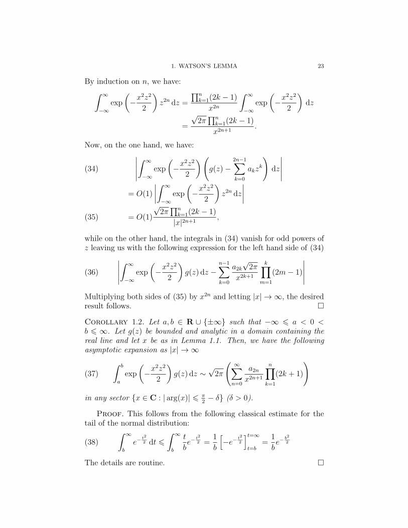
∣∣∣∣∣Multiplying both sides of (35) by x2n and letting |x| → ∞, the desiredresult follows.
Corollary 1.2. Let a, b ∈ R ∪ ±∞ such that −∞ ⩽ a < 0 <b ⩽ ∞. Let g(z) be bounded and analytic in a domain containing thereal line and let x be as in Lemma 1.1. Then, we have the followingasymptotic expansion as |x| → ∞
(37)
∫ b
a
exp
(−x
2z2
2
)g(z) dz ∼
√2π
(∞∑n=0
a2nx2n+1
n∏k=1
(2k + 1)
)
in any sector x ∈ C : | arg(x)| ⩽ π2− δ (δ > 0).
Proof. This follows from the following classical estimate for thetail of the normal distribution:
(38)
∫ ∞
b
e−t2
2 dt ⩽∫ ∞
b
t
be−
t2
2 =1
b
[−e−
t2
2
]t=∞
t=b=
1
be−
b2
2
The details are routine.
242. ASYMPTOTIC METHODS FOR INTEGRALS DEPENDING ON A LARGE PARAMETER
1.1. Examples.
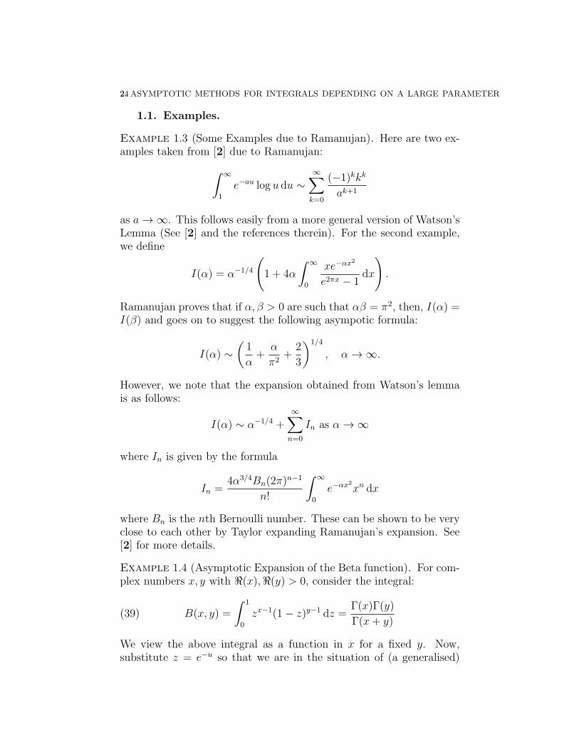
Example 1.3 (Some Examples due to Ramanujan). Here are two ex-amples taken from [2] due to Ramanujan:∫ ∞
1
e−au log u du ∼∞∑k=0
(−1)kkk
ak+1
as a→ ∞. This follows easily from a more general version of Watson’sLemma (See [2] and the references therein). For the second example,we define
I(α) = α−1/4
(1 + 4α
∫ ∞
0
xe−αx2
e2πx − 1dx
).
Ramanujan proves that if α, β > 0 are such that αβ = π2, then, I(α) =I(β) and goes on to suggest the following asympotic formula:
I(α) ∼(1
α+α
π2+
2
3
)1/4
, α → ∞.
However, we note that the expansion obtained from Watson’s lemmais as follows:
I(α) ∼ α−1/4 +∞∑n=0
In as α→ ∞
where In is given by the formula
In =4α3/4Bn(2π)
n−1
n!
∫ ∞
0
e−αx2
xn dx
where Bn is the nth Bernoulli number. These can be shown to be veryclose to each other by Taylor expanding Ramanujan’s expansion. See[2] for more details.
Example 1.4 (Asymptotic Expansion of the Beta function). For com-plex numbers x, y with ℜ(x),ℜ(y) > 0, consider the integral:
(39) B(x, y) =
∫ 1
0
zx−1(1− z)y−1 dz =Γ(x)Γ(y)
Γ(x+ y)
We view the above integral as a function in x for a fixed y. Now,substitute z = e−u so that we are in the situation of (a generalised)
2. LAPLACE’S METHOD 25
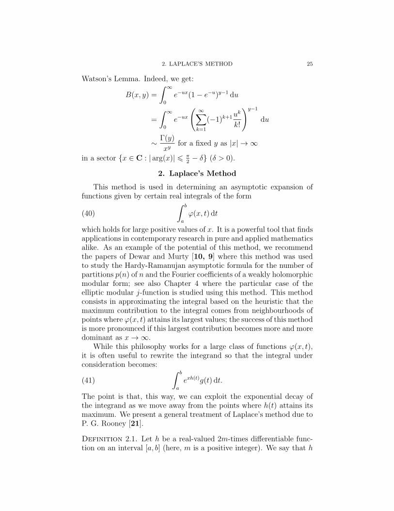
Watson’s Lemma. Indeed, we get:
B(x, y) =
∫ ∞
0
e−ux(1− e−u)y−1 du
=
∫ ∞
0
e−ux
(∞∑k=1
(−1)k+1uk
k!
)y−1
du
∼ Γ(y)
xyfor a fixed y as |x| → ∞
in a sector x ∈ C : | arg(x)| ⩽ π2− δ (δ > 0).
2. Laplace’s Method
This method is used in determining an asymptotic expansion offunctions given by certain real integrals of the form
(40)
∫ b
a
φ(x, t) dt
which holds for large positive values of x. It is a powerful tool that findsapplications in contemporary research in pure and applied mathematicsalike. As an example of the potential of this method, we recommendthe papers of Dewar and Murty [10, 9] where this method was usedto study the Hardy-Ramanujan asymptotic formula for the number ofpartitions p(n) of n and the Fourier coefficients of a weakly holomorphicmodular form; see also Chapter 4 where the particular case of theelliptic modular j-function is studied using this method. This methodconsists in approximating the integral based on the heuristic that themaximum contribution to the integral comes from neighbourhoods ofpoints where φ(x, t) attains its largest values; the success of this methodis more pronounced if this largest contribution becomes more and moredominant as x→ ∞.
While this philosophy works for a large class of functions φ(x, t),it is often useful to rewrite the integrand so that the integral underconsideration becomes:
(41)
∫ b
a
exh(t)g(t) dt.
The point is that, this way, we can exploit the exponential decay ofthe integrand as we move away from the points where h(t) attains itsmaximum. We present a general treatment of Laplace’s method due toP. G. Rooney [21].
Definition 2.1. Let h be a real-valued 2m-times differentiable func-tion on an interval [a, b] (here, m is a positive integer). We say that h
262. ASYMPTOTIC METHODS FOR INTEGRALS DEPENDING ON A LARGE PARAMETER
has a flat maximum of order m if h(n)(a) = 0 for all 0 < n < 2m andh(2m)(a) < 0.
Theorem 2.2. Let a < b be real numbers. Let h : [a, b] → R be anon-increasing function which is C2m([a, a + η]) for some real numberη with 0 < η < b−a. Suppose that h has a flat maximum of order m ata. Suppose further that (x− a)ν |ϕ(x)| is integrable on [a, b] and ϕ(a+)exists. If ϕ(a+) = 0, then, we have the asymptotic formula as λ→ ∞:
I(λ) :=
∫ b
a
exp(λh(x))(x− a)νϕ(x) dx
∼ exp(λh(a))
((2m)!
−λh(2m)(a)
) ν+12m
Γ
(ν + 1
2m
)ϕ(a+)
2m(42)
Proof. Fix an ε such that 0 < ε < |h(2m)(a)|2
. By the definition of
ϕ(a+) and continuity of h(2m) at a, it follows that there exists a δ > 0such that whenever 0 < x− a < δ, it follows that
|ϕ(x)− ϕ(a+)| < ε and(43)
|h(2m)(x)− h(2m)(a)| < ε.(44)
We shall study the integral
I(λ) exp(−λh(a)) =∫ b
a
expλ(h(x)− h(a))(x− a)νϕ(x) dx
=
∫ a+δ
a
+
∫ b
a+δ
= I1 + I2 (say)(45)
and show the following:
(a) contribution I1 from the δ-neighbourhood of the maximumx = a matches with the formula (42);
(b) contribution I2 from outside the δ-neighbourhood of x = a isO(αλ) for 0 < α < 1 as λ→ ∞.
The integral I2 is particularly easy to estimate: indeed, since h isnon-increasing
|I2| ⩽ expλ(h(a+ δ)− h(a))∫ b
a
|ϕ(x)|(x− a)ν dx(46)
and our claim in (b) above follows.
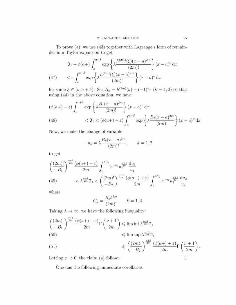
2. LAPLACE’S METHOD 27
To prove (a), we use (43) together with Lagrange’s form of remain-der in a Taylor expansion to get∣∣∣∣I1 − ϕ(a+)
∫ a+δ
a
exp
λh(2m)(ξ)(x− a)2m
(2m)!
(x− a)ν dx
∣∣∣∣< ε
∫ a+δ
a
exp
λh(2m)(ξ)(x− a)2m
(2m)!
(x− a)ν dx(47)
for some ξ ∈ (a, a + δ). Set Bk = h(2m)(a) + (−1)kε (k = 1, 2) so thatusing (44) in the above equation, we have:
(ϕ(a+)− ε)
∫ a+δ
a
exp
λB1(x− a)2m
(2m)!
(x− a)ν dx
< I1 < (ϕ(a+) + ε)
∫ a+δ
a
exp
λB2(x− a)2m
(2m)!
(x− a)ν dx(48)
Now, we make the change of variable
−uk = λBk(x− a)2m
(2m)!, k = 1, 2
to get((2m)!
−B1
) ν+12m (ϕ(a+)− ε)
2m
∫ λC1
0
e−u1uν+12m1
du1u1
< λν+12m I1 <
((2m)!
−B2
) ν+12m (ϕ(a+) + ε)
2m
∫ λC2
0
e−u2uν+12m2
du2u2
(49)
where
Ck =Bkδ
2m
(2m)!k = 1, 2.
Taking λ→ ∞, we have the following inequality:((2m)!
−B1
) ν+12m (ϕ(a+)− ε)
2mΓ
(ν + 1
2m
)⩽ lim inf λ
ν+12m I1
⩽ lim supλν+12m I1(50)
⩽((2m)!
−B2
) ν+12m (ϕ(a+) + ε)
2mΓ
(ν + 1
2m
).(51)
Letting ε→ 0, the claim (a) follows.
One has the following immediate corollaries:
282. ASYMPTOTIC METHODS FOR INTEGRALS DEPENDING ON A LARGE PARAMETER
Corollary 2.3. Let a < b be real numbers. Let h : [a, b] → R be anon-decreasing function which is C2m([b − η, b]) for some real numberη with 0 < η < b−a. Suppose that h has a flat maximum of order m atb. Suppose further that (b− x)ν |ϕ(x)| is integrable on [a, b] and ϕ(b−)exists. If ϕ(b−) = 0, then, we have the asymptotic formula as λ→ ∞:
J(λ) :=
∫ b
a
exp(λh(x))(b− x)νϕ(x) dx
∼ exp(λh(b))
((2m)!
−λh(2m)(b)
) ν+12m
Γ
(ν + 1
2m
)ϕ(b−)
2m(52)
Corollary 2.4. If all the hypotheses in our theorem hold but ϕ(a+) =0, then the asymptotic formula above is to be interpreted as the followingo-estimate:
I(λ) =
∫ b
a
exp(λh(x))(x− a)νϕ(x) dx = o
(exp(λh(a))
λν+12m
).(53)
The next corollary is an important variation on the main theoremthat we state it also as a theorem:
Theorem 2.5. Let a < ξ < b be real numbers. Let h : [a, b] → Rbe a C2m([ξ − η, ξ + η]) function for some real number η with 0 <η < min(b − ξ, ξ − a). Suppose that h has a flat maximum of orderm at ξ and that h has no other maxima in [a, b]. Suppose further that|x−ξ|ν |ϕ(x)| is integrable on [a, b] and ϕ(b+) and ϕ(b−) exist. If ϕ(b+)and ϕ(b−) are both non-zero, then, we have the asymptotic formula asλ→ ∞:
J(λ) :=
∫ b
a
exp(λh(x))(b− x)νϕ(x) dx
∼ exp(λh(b))
((2m)!
−λh(2m)(b)
) ν+12m
Γ
(ν + 1
2m
)ϕ(b+) + ϕ(b−)
2m(54)
Proof. We break the integral J at ξ so that J =∫ b
a=∫ ξ
a+∫ b
ξ.
An application of Corollary 2.3 and Theorem 2.2 respectively to thefirst and second piece gives the claim.
2.1. An Example.
Example 2.6. The modified Bessel function In(x) of order n has thefollowing integral representation
In(x) =1
π
∫ π
0
expx cos t cos(nt) dt
3. THE METHOD OF STEEPEST DESCENT 29
The integral is amenable to Laplace’s method: in fact, our theoremreadily gives the asymptotic formula
(55) In(x) ∼1√2πx
ex
as x→ ∞. (Of course, one uses the fact that Γ(1/2) =√π.)
3. The Method of Steepest Descent
The method of steepest descent (sometimes also known as the sad-dle point method) is an extension of Laplace’s method to the complexplane.
Let Ω be a simply connected domain in C. Let f and g be twoholomorphic functions on Ω and let γ : [0, 1] → Ω be a piecewise differ-entiable curve in Ω. The method of steepest descent aids in derivingan asymptotic formula for integrals the form
(56) F (t) =
∫γ
etf(ξ)g(ξ) dξ
for large positive values of t. For ξ = x + iy, write f(ξ) = u(x, y) +iv(x, y). If we are to appeal to Laplace’s philosophy, since |etf(ξ)| =etu(x,y), we should seek to deform the contour γ to another contourγ′ in Ω which consists of points (x0, y0) where u(x, y) is large. Notefirst that this deformation does not change the value of the integral asthe integrand is analytic in Ω (Cauchy’s theorem). However, the keydifficulty that we are presented with is as follows: “heuristically”, wesee that for large values of t, the function eitv(x,y) might oscillate rapidlyeven for small displacements along the curve γ′ that the positive andnegative swings in the values taken by the function will tend to cancelout.
However, this suggests that there is a reasonable chance of successif we can find a contour γ′ such that etu attains large values on thoseparts of the contour where v is constant and whenever v varies, themagnitude etu is small. One can argue that on a path where v isconstant and u attains its maximum at an interior point, say z0, wemust have that f ′(z0) = 0. Thus, we seek a contour γ′ such that:
(1) γ′ passes through one or more zeroes of f ′(z).(2) v(x, y) is constant on γ′.
A few remarks are in order about the choice of γ′. Consider the surfaceS(x, y, u(x, y)) in R3. If z0 = x0 + iy0 is a zero of f ′(z), then, Cauchy-Riemann equations
(57) f ′(z) = ux − iuy
302. ASYMPTOTIC METHODS FOR INTEGRALS DEPENDING ON A LARGE PARAMETER
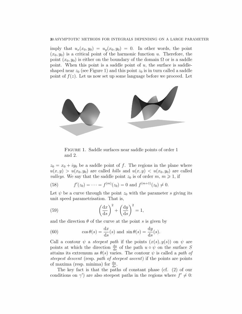
imply that ux(x0, y0) = uy(x0, y0) = 0. In other words, the point(x0, y0) is a critical point of the harmonic function u. Therefore, thepoint (x0, y0) is either on the boundary of the domain Ω or is a saddlepoint. When this point is a saddle point of u, the surface is saddle-shaped near z0 (see Figure 1) and this point z0 is in turn called a saddlepoint of f(z). Let us now set up some language before we proceed. Let
Figure 1. Saddle surfaces near saddle points of order 1and 2.
z0 = x0 + iy0 be a saddle point of f . The regions in the plane whereu(x, y) > u(x0, y0) are called hills and u(x, y) < u(x0, y0) are calledvalleys. We say that the saddle point z0 is of order m, m ⩾ 1, if
(58) f ′(z0) = · · · = f (m)(z0) = 0 and f (m+1)(z0) = 0.
Let ψ be a curve through the point z0 with the parameter s giving itsunit speed parametrisation. That is,
(59)
(dx
ds
)2
+
(dy
ds
)2
= 1,
and the direction θ of the curve at the point s is given by
(60) cos θ(s) =dx
ds(s) and sin θ(s) =
dy
ds(s).
Call a contour ψ a steepest path if the points (x(s), y(s)) on ψ arepoints at which the direction du
dsof the path u ψ on the surface S
attains its extremum as θ(s) varies. The contour ψ is called a path ofsteepest descent (resp. path of steepest ascent) if the points are pointsof maxima (resp. minima) for du
ds.
The key fact is that the paths of constant phase (cf. (2) of ourconditions on γ′) are also steepest paths in the regions where f ′ = 0:
3. THE METHOD OF STEEPEST DESCENT 31
indeed,
(61)du
ds= cos θ
∂u
∂x+ sin θ
∂u
∂y
attains its extrema at points where the derivative of duds
with respect toθ
(62) − sin θ∂u
∂x+ cos θ
∂u
∂y= − sin θ
∂v
∂y− cos θ
∂v
∂x= −dv
ds
vanishes and the second derivative of duds
with respect to θ
(63) − cos θ∂u
∂x− sin θ
∂u
∂y=
du
ds
is non-zero. Note further that γ′ is a path of steepest ascent (resp.descent) if du
ds> 0 (resp. du
ds< 0).
Remark 3.1. The discussion above can also be paraphrased in termsof gradient of multivariate function: a path ψ would then be calleda steepest path if the tangent vector (dx
ds, dyds) at s of the path ψ is
parallel to ∇u at ψ(s); equivalently, we require that the normal vector(−dy
ds, dxds) and ∇u are perpendicular (cf. (62)).
Suppose now that z0 is a saddle point of order m, m ⩾ 1. Then,the Taylor expansion of f at z = z0 + reiθ around z0 is given by
(64) f(z) = f(z0) +rm+1
(m+ 1)!ai(m+1)θ+φ + · · ·
where we have let f (m+1)(z0) = aeiφ (a > 0). This gives us:
• the direction of the curves v(x, y) = v(x0, y0) of constant phaseat z0, viz, the solutions to the equation sin((m+1)θ+φ) = 0:
(65) θ =1
m+ 1(−φ+ kπ), k = 0, . . . , 2m+ 1
• the direction of the level curves of u, viz, the solutions to theequation cos((m− 1)θ + φ) = 0:
(66) θ =1
m+ 1
(−φ+ (2k + 1)
π
2
), k = 0, . . . , 2m+ 1.
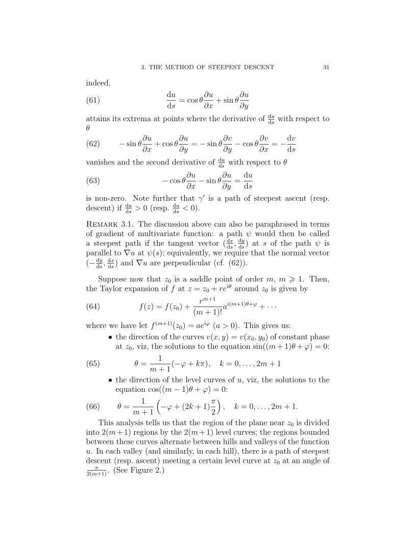
This analysis tells us that the region of the plane near z0 is dividedinto 2(m+1) regions by the 2(m+1) level curves; the regions boundedbetween these curves alternate between hills and valleys of the functionu. In each valley (and similarly, in each hill), there is a path of steepestdescent (resp. ascent) meeting a certain level curve at z0 at an angle of
π2(m+1)
. (See Figure 2.)
322. ASYMPTOTIC METHODS FOR INTEGRALS DEPENDING ON A LARGE PARAMETER
Figure 2. Lines of constant phase (solid) and levelcurves of u (dotted) near saddle points of order 1 and2.
Suppose now that γ′ is a steepest path through z0. Then, the realpart is either monotonically increasing to or decreasing from u(x0, y0)on this path γ′. The paths γ′ lying in valleys (viz, those along which udecreases) are paths of steepest decent.
The thesis of the method of steepest descents is the following: byTaylor expanding f near a saddle point z0, the expansion obtained byterm-wise integration is asymptotic if we can shift our contour γ to acontour γ′ lying in valleys and passing through a saddle point betweenvalleys.
3.1. Contribution from a saddle point. Throughout what fol-lows, we shall assume that z0 is a saddle point of order 1 for f . Thekey feature of this assumption is that, in this case, there are two pathsof steepest descent at an angle of ±π from each other (so oppositelydirected rays emanating from z0).
Expanding f in Taylor series around z0, we have (since f′(z0) = 0):
(67) f(z) = f(z0) +f ′′(z0)
2!(z − z0)
2 + · · · .
We cut down to a small neighbourhood of z0 in which
f1(z) :=f(z)− f(z0)
(z − z0)2
is analytic. If γ is the part of the curve γ in this neighbourhood, then,the saddle point z0 contributes
(68)
∫γ
exp(tf1(z0)(z − z0)
2)g(z) dz
to the integral (56). Since (z − z0)2f ′′(z0) is real and negative on a
path of the steepest descent, we put −12ζ2 = f1(z)(z− z0)
2 so that ζ is
3. THE METHOD OF STEEPEST DESCENT 33
determined as the principal value of the square root of the appropriatequantity. This change of variable leaves us with:
(69) etf(z0)∫γ
exp
(−1
2ζ2)g(z)
dz
dζdζ.
This puts us in the situation of Watson’s lemma showing the existenceof an asymptotic expansion. Now, we are faced with the problem ofinverting the given power series ζ(z) to get z(ζ). This is usually cum-bersome.
However, getting just the leading term in the series z(ζ) is nothard and gives us the first term of the asymptotic expansion (Watson’slemma). Write z − z0 = r(z)e−iφ (recall that φ = arg(f ′′(z0))) so that
ζ = ±r√|f ′′(z0)| (the correct sign being given by the sign of the rate
of change of the real part on γ: thus, + would be the right sign if thereal part is increasing and − otherwise). Via Watson’s Lemma, weconclude that the amount I(z0) contributed by the saddle point z0 is
(70) I(z0) = ±g(z0)etf(z0)
√2πe−iφ√
|tf ′′(z0)|This completes our discussion of the saddle point method.
CHAPTER 3
Two Examples
In this chapter, we present a proof of Stirling’s formula for thecomplex Gamma function and explore the technique of using Mellintransforms to obtain asymptotic formulas.
1. Stirling’s formula for the complex Gamma function
We apply the method of steepest descent to the complex Gammafunction defined as follows:
(71) Γ(z + 1) :=
∫ ∞
0
e−ssz ds, for ℜ(z) > −1.
We rewrite the integrand so that we have:
(72) Γ(z + 1) =
∫ ∞
0
e−s+z ln s ds.
For z ∈ C with ℜ(z) > 0, put s = z(1 + t) so that ds = zdt and:
Γ(z + 1) = zz+1e−z
∫ ∞
−1
exp(−tz + z ln(1 + t)) dt.(73)
Now, analysing the function f(t) = ln(1 + t)− t, we see that the onlysaddle point t = 0 of order 1 has the property that f ′′(0) = −1. In thiscase, the real line is already a path of steepest descent and the sign inI(0) given by the contour is +. Putting these facts together, we have
(74) I(0) =√2π/z.
This gives us the Stirling’s formula for the complex Gamma function
(75) Γ(z + 1) ∼√2πz
(ze
)zwhen |z| → ∞ in any sector z ∈ C : | arg(z)| ⩽ π
2− δ < π
2.
35
36 3. TWO EXAMPLES
2. The Mellin transform and its application to asymptotics
In this section, following Flajolet et. al. [11], we expose a techniqueintroduced by De Bruijn and Knuth to obtain asymptotic formula forthe sums of the form
(76) G(x) =∑k
λkg(µkx)
where g is a continuous function. These sums are called harmonic sumssince one may view G as the linear superposition of “harmonics” of thefunction g; in view of this analogy, one calls λk’s the amplitudes andµk’s the frequencies of the harmonic sum.
This technique uses the Mellin transform which we briefly review.
2.1. The Mellin transform. Let us begin with the followinglemma:
Lemma 2.1. Let f be a locally integrable complex-valued function de-fined on (0,∞). Suppose further that
f(x) =
O(xα), as x→ 0
O(xβ), as x→ ∞.(77)
Then the integral
f ∗(s) =
∫ ∞
0
f(x)xsdx
x(78)
converges for all s such that −α < ℜ(s) < −β and defines an analyticfunction in this (possibly empty!) strip.
Proof. This is obvious: break the integral∫∞0
=∫ 1
0+∫∞1, esti-
mate using (77):∣∣∣∣∫ ∞
0
f(x)xsdx
x
∣∣∣∣ ⩽ ∫ 1
0
|f(x)xs| dx|x|
+
∫ ∞
1
|f(x)xs| dx|x|∫ 1
0
xℜ(s)+α−1 dx+
∫ ∞
1
xℜ(s)+β−1 dx
Since the integrals in the last step are convergent in −α < ℜ(s) < −β,the first claim follows. For the second claim, we may use Morera’stheorem together with absolute convergence of the integral in the saidregion.
We introduce the notation ⟨a, b⟩ to denote the vertical open stripa < ℜ(s) < b. In view of this lemma, it is appropriate to make thefollowing definition:
2. THE MELLIN ASYMPTOTICS 37
Definition 2.2. Let f be a locally integrable complex-valued functiondefined on (0,∞) satisfying (77). Then, the function f ∗(s) is called theMellin transform of f and the largest open strip on which f ∗ is definedis called its the fundamental strip.
We now list some important functional properties of this transform,easily proven using change of variables.
Theorem 2.3. Let g be a locally integrable complex-valued functionwith Mellin transform g∗. Suppose that g∗ has the fundamental strip⟨α, β⟩. Then:
Function Mellin Transform Fundamental Stripg(x) g∗(s) ⟨α, β⟩
We close this section with an extension of the last entry in our tableto handle infinite harmonic sums.
Theorem 2.4. Suppose that g is a locally integrable complex valuedfunction on (0,∞). Consider the harmonic sum (76) and put Λ for theDirichlet series
(79) Λ(s) =∑k
λkµsk
If the halfplane on which Λ is convergent has a non-empty intersectionwith the fundamental strip of g∗, then, G(x) exists for all x and theidentity G∗(s) = Λ(s)g∗(s) holds in the intersection.
2.2. The fundamental correspondence. We now have the fun-damental correspondence which states that associated to each pole off ∗(s) there corresponds a term in the asymptotic expansion as x→ ∞.
Theorem 2.5. Let f be r-times differentiable function on (0,∞) withr ⩾ 2. Suppose that f ∗ has the non-empty fundamental strip ⟨α, β⟩ andcan be meromorphically continued to ⟨β, η⟩ for some η > β. Supposethat f ∗ is analytic in a domain containing ℜ(s) = η and that f ∗ hasonly finitely many poles with real part < η. Then, we have the following
38 3. TWO EXAMPLES
asymptotic formula:
f(x) =∑
(ξ,k)∈A
dξ,k
((−1)k−1
(k − 1)!x−ξ(log x)k
)+O(x−η), x→ ∞(80)
where the sum runs over the real parts ξ of the poles of f ∗ and theirmultiplicities k; here dξ,k is the residue of the respective pole.
Proof. See [11, Theorem 4]. The remarkable feature is that this correspondence is also reversible.
In fact, if one assumes an asymptotic expansion upto a certain orderfor f , then, one may obtain a meromorphic continuation for f ∗ and adescription of the location of the poles and their respective residues.See [11, 26] for more details.
We close this section with the following remark:
Remark 2.6. The fundamental correspondence given in Theorem 2.5can be generalised so as to study continuous functions f for which f ∗
admits a singular expansion. See [11] for more details.
2.3. Application to Harmonic sums. The key theorem in thissection is the following asymptotic expansion for a harmonic sum asx→ ∞.
Theorem 2.7. Consider the harmonic sum (76) which is assumed tobe convergent for all x ∈ (0,∞). Assume that G∗ satisfies the hypothe-ses of the theorem 2.5. Then, we have the following asymptotic formulaas x→ ∞:
G(x) =∑
(ξ,k)∈A
dξ,k
((−1)k−1
(k − 1)!x−ξ(log x)k
)+O(x−η), x→ ∞(81)
where the sum runs over the real parts ξ of the poles of g∗ and theirmultiplicities k; here dξ,k is the residue of the pole.
Proof. See [11, Section 3, Theorem 5].
CHAPTER 4
On the asymptotic formula for the Fouriercoefficients of j-function
The contents of this chapter are joint with Ram Murty. This workwill appear in Kyushu Math Journal under this same title.
1. Preliminaries
In this section, we shall set up the notation and review the keyingredients necessary for the proof.
The first fact we need is a well-known fact about binary quadraticforms (see [12, Chapter 6] for an introduction). We shall write [a, b, c]for the form aX2 + bXY + cY 2. The discriminant of the form [a, b, c]is b2 − 4ac, consequently, the discriminant of any form is 0 or 1 mod 4accordingly as b is even or odd.
Definition 1.1 (Principal form of discriminant D). The binary qua-dratic form
(82) ID =
[1, 0,−D
4
], D ≡ 0 mod 4[
1, 1, 1−D4
], D ≡ 1 mod 4
is a form with discriminant D and is called the principal form of dis-criminant D.
Recall that a form P is said to represent an integer m if there arex, y ∈ Z such that P (x, y) = m. The following lemma offers a keysimplification to our proof:
Lemma 1.2. The following are equivalent for a form P of discriminantD:
(i) P represents 1.(ii) P is SL2(Z)-equivalent to [1, B, C] for some B,C ∈ Z.(iii) P is SL2(Z)-equivalent to the principal form of discriminant
D.
Proof.(i) =⇒ (ii): Suppose that x and y are integers such that P (x, y) = 1.
39
40 4. THE FOURIER COEFFICIENTS OF j-FUNCTION
Then, we have that (x, y) = 1; so there are integers r, s such thatxr− ys = 1. Putting p for the matrix corresponding to P , we see that(
x sy r
)t
p
(x sy r
)=
(P (x, y) ∗
∗ P (s, r)
)=
(1 ∗∗ P (s, r)
)as required.(ii) =⇒ (iii): The equations:(
1 0−B
21
)(1 B
2B2
C
)(1 −B
20 1
)=
(1 0
0 4C−B2
4
), when B is even(
1 0−B−1
21
)(1 B
2B2
C
)(1 −B−1
20 1
)=
(1 1
212
14+ 4C−B2
4
), when B is odd
establish the claim.(iii) =⇒ (i): Let iD (resp. p) denote the matrix corresponding tothe principal form (resp. P ). Then, there exists S ∈ SL2(Z) such thatStiDS = p. We note that:(
1 0)(S−1)tpS−1
(10
)=(1 0
)iD
(10
)= 1
so that P represents 1 as claimed.
We now review Kaneko’s arithmetic formula for c(n), one of the keyingredients in our proof:
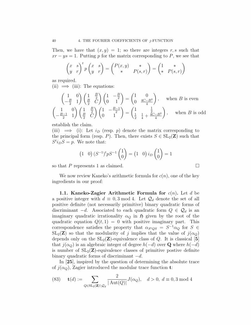
1.1. Kaneko-Zagier Arithmetic Formula for c(n). Let d bea positive integer with d ≡ 0, 3 mod 4. Let Qd denote the set of allpositive definite (not necessarily primitive) binary quadratic forms ofdiscriminant −d. Associated to each quadratic form Q ∈ Qd is animaginary quadratic irrationality αQ in H given by the root of thequadratic equation Q(t, 1) = 0 with positive imaginary part. Thiscorrespondence satisfies the property that αStQS = S−1αQ for S ∈SL2(Z) so that the modularity of j implies that the value of j(αQ)depends only on the SL2(Z)-equivalence class of Q. It is classical [5]that j(αQ) is an algebraic integer of degree h(−d) over Q where h(−d)is number of SL2(Z)-equivalence classes of primitive postive definitebinary quadratic forms of discriminant −d.
In [25], inspired by the question of determining the absolute traceof j(αQ), Zagier introduced the modular trace function t:
(83) t(d) :=∑
Q∈SL2(Z)\Qd
2
|Aut(Q)|J(αQ), d > 0, d ≡ 0, 3 mod 4
2. ASYMPTOTIC FORMULA FOR j(τ) 41
for the normalised Hauptmodul J(τ) := j(τ) − 744 for SL2(Z). Also,for convenience, define t(0) = 2 and t(−1) = −1 and set t(d) = 0 ifd ≡ 1, 2 mod 4 or if d < −1.
Recall the well-known fact about automorphs of binary quadraticforms ([12, Theorem 6.1.9]):
(84) |Aut(Q)| =
6, Q ∼ [a, a, a]
4, Q ∼ [a, 0, a]
2, otherwise.
Based on Zagier’s theorems, Kaneko [15] gave a closed form expres-sion for the coefficients c(n) of the j-function:
Theorem 1.3 (Kaneko). For any n ⩾ 1, we have that(85)
c(n) =1
n
∑r∈Z
t(n− r2) +∑
r⩾1, r odd
((−1)nt(4n− r2)− t(16n− r2))
.
2. Asymptotic formula for j(τ)
In this section, we shall prove (1) using Kaneko’s arithmetic formula(85). We begin by noting that the contribution to t(d) comes only fromI−d.
Lemma 2.1. With notations as before, we have the following asymp-totic formula:
(86) c(n) ∼ 1
n
∑1⩽r⩽
√16n−1
r odd
eπ√16n−r2
as n→ ∞.
Proof. In view of Kaneko’s formula (85), let us analyse the mod-ular trace t(d), d > 0 to get started: recall from (83) that
t(d) =∑
Q∈SL2(Z)\Qd
2
|Aut(Q)|J(αQ).
We claim that the only class that contributes to this sum is the class[I−d]. Indeed, if Q = [a, b, c] is a form of discriminant −d, then, wehave:
e2πiαQ = exp
(2πi
(−b+ i
√d
2a
))= exp
(−πib
a
)exp
(−π
√d
a
)
42 4. THE FOURIER COEFFICIENTS OF j-FUNCTION
and consequently:
J(αQ) = j(αQ)− 744
= q−1 +O(q)
= exp
(πib
a
)exp
(π√d
a
)+O
(exp
(−π
√d
a
)).
In view of this, the contribution to t(d) comes only from classes thathave forms with a = 1. By Lemma 1.2, any such form is equivalent tothe principal form I−d so that we have:
(87) t(d) = O(exp(−π√d)) +
exp(π
√d), d ≡ 0 mod 4, d = 4
− exp(π√d), d ≡ 3 mod 4, d = 3
.
Since eπ√n = o(e4π
√n) and e2π
√n = o(e4π
√n), the contribution to c(n)
comes only from the last summand of the formula. Since 16n − r2 ≡3 mod 4 when r is odd, the claim follows from (85) and (87) on amoment’s reflection.
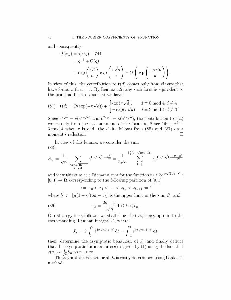
In view of this lemma, we consider the sum(88)
Sn :=1√n
∑1⩽r⩽
√16n−1
r odd
e4π√n
√1− r2
16n =1
2√n
⌊ 12(1+
√16n−1)⌋∑
k=1
2e4π√n
√1− (2k−1)2
16n
and view this sum as a Riemann sum for the function t 7→ 2e4π√n√1−t2 :
[0, 1] → R corresponding to the following partition of [0, 1]:
0 =: x0 < x1 < · · · < xbn < xbn+1 := 1
where bn := ⌊12(1 +
√16n− 1)⌋ is the upper limit in the sum Sn and
(89) xk =2k − 1
4√n, 1 ⩽ k ⩽ bn.
Our strategy is as follows: we shall show that Sn is asymptotic to thecorresponding Riemann integral Jn where
Jn := 2
∫ 1
0
e4π√n√1−t2 dt =
∫ 1
−1
e4π√n√1−t2 dt;
then, determine the asymptotic behaviour of Jn and finally deducethat the asymptotic formula for c(n) is given by (1) using the fact thatc(n) ∼ 1√
nSn as n→ ∞.
The asymptotic behaviour of Jn is easily determined using Laplace’smethod:
2. ASYMPTOTIC FORMULA FOR j(τ) 43
Lemma 2.2. We have the following asymptotic formula
(90) Jn ∼ e4π√n
√2n1/4
as n→ ∞.
Proof. We apply Theorem 2.5 from Chapter 2 to our integralwith the obvious candidate function: put h(t) = 4π
√1− t2 on (−1, 1).
Then, the function h has a unique maximum at ξ = 0. Its first twoderivatives are given by:
h′(t) = −4πt√
1− t2and h′′(t) =
−4π
(1− t2)3/2
and (54) gives the claim.
Corollary 2.3. We have the following asymptotic formula
(91)1√nJn ∼ e4π
√n
√2n3/4
as n→ ∞.
This corollary leaves us with showing that Sn ∼ Jn as n→ ∞. Thisis done in the following lemma:
Lemma 2.4. With notations as before, we have that:
(92) limn→∞
∣∣∣∣Sn
Jn− 1
∣∣∣∣ = 0.
In other words, the sum Sn is asymptotic to the integral Jn.
Proof. Let f be the function defined on [0, 1] by f(x) = 2e4π√n√1−x2
.
Then f is a decreasing function. Let b := bn = ⌊1+√16n−12
⌋ denote theupper limit in Sn. We estimate the difference Sn − Jn (with xk as in(89)):
Sn − Jn
=1
2√n
b∑k=1
f(xk)−∫ 1
0
f(t) dt
=
(1
2√nf(x1)−
∫ x1
0
f(t) dt
)+
b∑k=2
∫ xk
xk−1
(f(xk)− f(t)) dt−∫ 1
xb
f(t) dt
= Σ1(n) + Σ2(n) + Σ3(n) (say).
44 4. THE FOURIER COEFFICIENTS OF j-FUNCTION
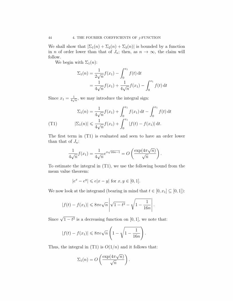
We shall show that |Σ1(n) + Σ2(n) + Σ3(n)| is bounded by a functionin n of order lower than that of Jn; then, as n → ∞, the claim willfollow.
We begin with Σ1(n):
Σ1(n) =1
2√nf(x1)−
∫ x1
0
f(t) dt
=1
4√nf(x1) +
1
4√nf(x1)−
∫ x1
0
f(t) dt
Since x1 =1
4√n, we may introduce the integral sign:
Σ1(n) =1
4√nf(x1) +
∫ x1
0
f(x1) dt−∫ x1
0
f(t) dt
|Σ1(n)| ⩽1
4√nf(x1) +
∫ x1
0
|f(t)− f(x1)| dt.(T1)
The first term in (T1) is evaluated and seen to have an order lowerthan that of Jn:
1
4√nf(x1) =
1
4√neπ
√16n−1 = O
(exp(4π
√n)√
n
).
To estimate the integral in (T1), we use the following bound from themean value theorem:
|ex − ey| ⩽ e|x− y| for x, y ∈ [0, 1].
We now look at the integrand (bearing in mind that t ∈ [0, x1] ⊆ [0, 1]):
|f(t)− f(x1)| ⩽ 8πe√n
∣∣∣∣∣√1− t2 −√
1− 1
16n
∣∣∣∣∣ .Since
√1− t2 is a decreasing function on [0, 1], we note that:
|f(t)− f(x1)| ⩽ 8πe√n
(1−
√1− 1
16n
).
Thus, the integral in (T1) is O(1/n) and it follows that:
Σ1(n) = O
(exp(4π
√n)√
n
).
2. ASYMPTOTIC FORMULA FOR j(τ) 45
This completes the analysis of the sum Σ1(n). We study the sum Σ2(n):
|Σ2(n)| ⩽b∑
k=2
∫ xk
xk−1
|f(xk)− f(t)| dt.(T2)
As before, we study the integrand:
|f(t)− f(xk)| ⩽ 8πe√n
∣∣∣∣√1− t2 −√1− x2k
∣∣∣∣⩽ 8πe
√n
(√1− x2k−1 −
√1− x2k
)Using the inequality 1− x
2− x2
2⩽
√1− x ⩽ 1− x
2, we get:
|f(t)− f(xk)| ⩽ 4πe√n(x4k + x2k − x2k−1)
In view of equation (T2), we have:
|Σ2(n)| ⩽ 2πe
(b∑
k=2
x4k +b∑
k=2
(x2k − x2k−1)
)
= 2πe
(1
256n2
b∑k=2
(2k − 1)4 + x2b − x21
)
⩽ 2πe
(1
256n2
b∑k=2
(2k − 1)4 +8n− 1
8n
)
which is indeed bounded by a rational function in n. Let us now con-sider Σ3(n):
Σ3(n) = −∫ 1
xb
f(t) dt
|Σ3(n)| ⩽ 2
∫ 1
xb
e4π√n√1−t2 dt.(T3)
For x ∈ R, writing x for the fractional part x − ⌊x⌋ of x, we notethat
1 +√16n− 1
2
⩽ max
(1
2+
√16n− 12
,√16n− 12
)=
1
2+
√16n− 12
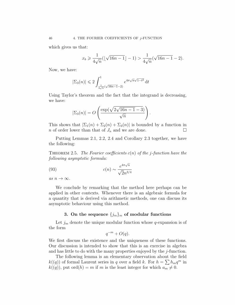
46 4. THE FOURIER COEFFICIENTS OF j-FUNCTION
which gives us that:
xb ⩾1
4√n(⌊√16n− 1⌋ − 1) >
1
4√n(√16n− 1− 2).
Now, we have:
|Σ3(n)| ⩽ 2
∫ 1
14√n(√16n−1−2)
e4π√n√1−t2 dt
Using Taylor’s theorem and the fact that the integrand is decreasing,we have:
|Σ3(n)| = O
(exp(
√2√16n− 1− 3)√n
).
This shows that |Σ1(n) + Σ2(n) + Σ3(n)| is bounded by a function inn of order lower than that of Jn and we are done.
Putting Lemmas 2.1, 2.2, 2.4 and Corollary 2.3 together, we havethe following:
Theorem 2.5. The Fourier coefficients c(n) of the j-function have thefollowing asymptotic formula:
(93) c(n) ∼ e4π√n
√2n3/4
as n→ ∞.
We conclude by remarking that the method here perhaps can beapplied in other contexts. Whenever there is an algebraic formula fora quantity that is derived via arithmetic methods, one can discuss itsasymptotic behaviour using this method.
3. On the sequence jmm of modular functions
Let jm denote the unique modular function whose q-expansion is ofthe form
q−m +O(q).
We first discuss the existence and the uniqueness of these functions.Our discussion is intended to show that this is an exercise in algebraand has little to do with the many properties enjoyed by the j-function.
The following lemma is an elementary observation about the fieldk((q)) of formal Laurent series in q over a field k. For h =
∑hmq
m ink((q)), put ord(h) = m if m is the least integer for which am = 0.
3. ON THE SEQUENCE jmm OF MODULAR FUNCTIONS 47
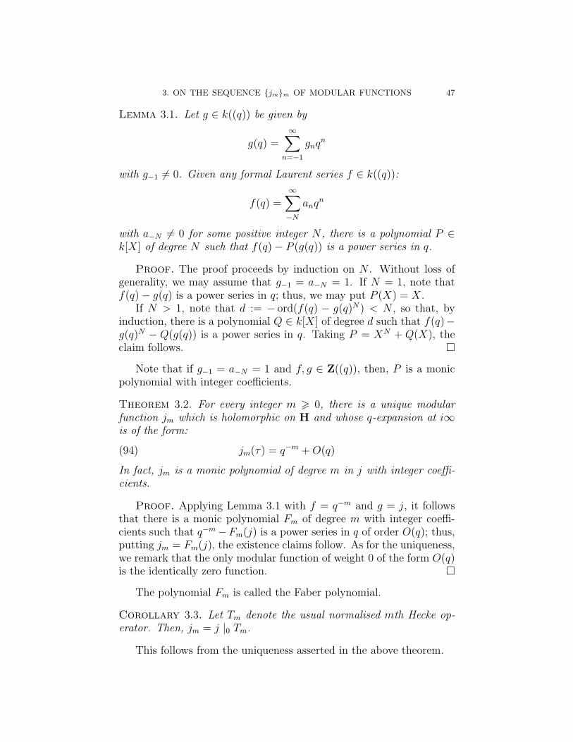
Lemma 3.1. Let g ∈ k((q)) be given by
g(q) =∞∑
n=−1
gnqn
with g−1 = 0. Given any formal Laurent series f ∈ k((q)):
f(q) =∞∑−N
anqn
with a−N = 0 for some positive integer N , there is a polynomial P ∈k[X] of degree N such that f(q)− P (g(q)) is a power series in q.
Proof. The proof proceeds by induction on N . Without loss ofgenerality, we may assume that g−1 = a−N = 1. If N = 1, note thatf(q)− g(q) is a power series in q; thus, we may put P (X) = X.
If N > 1, note that d := − ord(f(q) − g(q)N) < N , so that, byinduction, there is a polynomial Q ∈ k[X] of degree d such that f(q)−g(q)N − Q(g(q)) is a power series in q. Taking P = XN + Q(X), theclaim follows.
Note that if g−1 = a−N = 1 and f, g ∈ Z((q)), then, P is a monicpolynomial with integer coefficients.
Theorem 3.2. For every integer m ⩾ 0, there is a unique modularfunction jm which is holomorphic on H and whose q-expansion at i∞is of the form:
(94) jm(τ) = q−m +O(q)
In fact, jm is a monic polynomial of degree m in j with integer coeffi-cients.
Proof. Applying Lemma 3.1 with f = q−m and g = j, it followsthat there is a monic polynomial Fm of degree m with integer coeffi-cients such that q−m −Fm(j) is a power series in q of order O(q); thus,putting jm = Fm(j), the existence claims follow. As for the uniqueness,we remark that the only modular function of weight 0 of the form O(q)is the identically zero function.
The polynomial Fm is called the Faber polynomial.
Corollary 3.3. Let Tm denote the usual normalised mth Hecke op-erator. Then, jm = j |0 Tm.
This follows from the uniqueness asserted in the above theorem.
48 4. THE FOURIER COEFFICIENTS OF j-FUNCTION
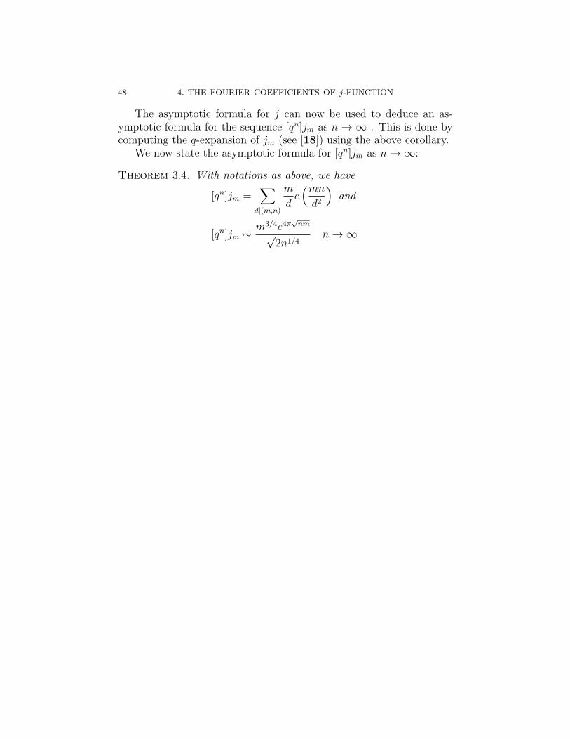
The asymptotic formula for j can now be used to deduce an as-ymptotic formula for the sequence [qn]jm as n → ∞ . This is done bycomputing the q-expansion of jm (see [18]) using the above corollary.
We now state the asymptotic formula for [qn]jm as n→ ∞:
Theorem 3.4. With notations as above, we have
[qn]jm =∑
d|(m,n)
m
dc(mnd2
)and
[qn]jm ∼ m3/4e4π√nm
√2n1/4
n→ ∞
Bibliography
[1] Carl M. Bender and Steven A. Orszag. Advanced Mathematical Methods forScientists and Engineers I: Asymptotic Methods and Perturbation Theory.Springer-Verlag, 1978.
[2] Bruce C. Berndt and Ronald J. Evans. Some elegant approximations and as-ymptotic formulas of Ramanujan. J. Comp. and App. Math., 37:35–41, 1991.
[3] Nicolas Brisebarre and Georges Philibert. Effective lower and upper boundsfor the Fourier coefficients of powers of the modular invariant j. J. RamanujanMath., 20(4):255–282, 2005.
[4] Jan Hendrik Bruinier and Ken Ono. Algebraic formulas for the coefficientsof half-integral weight harmonic weak Maass forms. Adv. Math., 246:198–219,2013.
[5] David A. Cox. Primes of the form x2+ny2. A Wiley-Interscience Publication.John Wiley & Sons, Inc., New York, 1989.
[6] Abraham de Moivre.Miscellanea Analytica de Seriebus et Quadraturis. Tousonand Watts, London, England, 1730.
[7] Abraham de Moivre. The Doctrine of Chances: Or, A Method of CalculatingProbabilities of Events in Play. A. Millar, London, England, Third edition,1756.
[8] P. Debye. Collected Works. Interscience Publishers, Inc., 1953.[9] M. Dewar and M. Ram Murty. An asymptotic formula for the coefficients of
j(z). International J. of Number Theory, 9(3):1–12, 2013.[10] Michael Dewar and M. Ram Murty. A derivation of the Hardy-Ramanujan
formula from an arithmetic formula. Proceedings of the American MathematicalSociety, 141:1903 – 1911, 2012.
[11] P. Flajolet, X. Gourdon, and P. Dumas. Mellin transform and asymptotics:Harmonic sums. Theoretical Computer Science, 144:3–58, 1995.
[12] Franz Halter-Koch. Quadratic Irrationals: An Introduction to Classical Num-ber Theory. CRC Press, Boca Raton, FL, 2013.
[13] G. H. Hardy and S. Ramanujan. Asymptotic formulae in combinatory analysis.Proc. London Math. Soc. (2), 17:75–115, 1918.
[14] A. E. Ingham. A Tauberian Theorem for Partitions. Ann. of Math. (2),42:1075–1090, 1941.
[15] Masanobu Kaneko. Traces of singular moduli and the Fourier coefficients ofthe elliptic modular function j(τ). In Number Theory (Ottawa, ON, 1996),volume 19 of CRM Proc. Lecture Notes, pages 173–176. Amer. Math. Soc.,Providence, RI, 1999.
[16] H. Petersson. Uber die Entwicklungskoeffizienten der automorphen Formen.Acta Math., 58(1):169–215, 1932.
49
50 BIBLIOGRAPHY
[17] H. Rademacher. The Fourier coefficients of the Modular Invariant J(τ). Amer.J. Math., 60(2):501–512, 1938.
[18] M. Ram Murty. Problems in the Theory of Modular Forms. IMSc LectureNotes, No. 1. Hindustan Book Agency, 2015.
[19] M. Ram Murty and Kannappan Sampath. A very simple proof of Stirling’sformula. The Mathematics Student, 84(1-2):129–133, May 2015.
[20] Bernhard Riemann. Gesammelte Mathematische Werke. Dover Publications,Inc., 1953.
[21] P. G. Rooney. Some Remarks on Laplace’s Method. Trans. Roy. Soc. Canada,XLVII:29–34, Jun 1953.
[22] Jean-Pierre Serre. A Course in Arithmetic. Graduate Texts in Mathematics,No. 7. Springer-Verlag, 1973.
[23] Ian Tweddle. James Stirling’s Methodus Differentialis: An Annotated Trans-lation of Stirling’s Text. Springer-Verlag, London, England, 2003.
[24] R. Wong. Asymptotic Approximations of Integrals. Computer Science and Sci-entific Computing. Academic Press, Inc., 1989.
[25] Don Zagier. Traces of singular moduli. In Motives, polylogarithms and Hodgetheory, Part I (Irvine, CA, 1998), volume 3 of Int. Press Lect. Ser., pages211–244. Int. Press, Somerville, MA, 2002.
[26] Don Zagier. The Mellin transform and other useful analytic techniques, chapterAppendix, pages 305–323. Springer-Verlag, Berlin-Heidelberg-New York, 2006.