44
State of Kansas 5-Year Ambient Air Monitoring Network Assessment October 16, 2015 Department of Health and Environment Division of Environment Bureau of Air (785) 296-6024

State of Kansas
5-Year Ambient Air Monitoring Network Assessment
October 16, 2015
Department of Health and Environment Division of Environment
Bureau of Air (785) 296-6024

ii
Table of Contents List of Tables ..................................................................................................................... iii List of Figures .................................................................................................................... iv Introduction ......................................................................................................................... 1 Kansas Weather .................................................................................................................. 1 Uses of Network Data ......................................................................................................... 2 Population Summary ........................................................................................................... 3
Metropolitan Statistical Areas......................................................................................... 3 Combined Statistical Areas ............................................................................................. 4 Micropolitan Statistical Areas......................................................................................... 4
Anticipated Growth/Decline ........................................................................................... 6 Kansas Criteria Pollutant Emissions Trends ....................................................................... 6 Current Criteria Emissions in Kansas ................................................................................. 7 Ozone Monitoring Network ................................................................................................ 9
Current Ozone Standard and Monitoring Requirements ................................................ 9 State of Kansas Current Ozone Monitoring Network ..................................................... 9 Ozone Measurements Trend Analysis .......................................................................... 10 Correlations between Kansas Ozone Monitors ............................................................. 14 Ozone Removal Bias Analysis...................................................................................... 15 Proposed Kansas Ozone Monitoring Network 2015-2020 ........................................... 16
PM2.5 Monitoring Network ............................................................................................... 17
Current PM2.5 Standard and Monitoring Requirements ................................................ 17 State of Kansas Current PM2.5 Monitoring Network .................................................... 18 PM2.5 Measurements Trend Analysis............................................................................ 19 Correlations between Kansas PM2.5 Monitors .............................................................. 23 PM2.5 Removal Bias Analysis ....................................................................................... 24 Proposed Kansas PM2.5 Monitoring Network 2015-2020 ............................................ 25
PM10 Monitoring Network ................................................................................................ 26 Current PM10 Standard and Monitoring Requirements ................................................ 26 State of Kansas Current PM10 Monitoring Network ..................................................... 27 PM10 Measurements Trend Analysis ............................................................................ 28 Proposed Kansas PM10 Monitoring Network 2015-2020 ............................................. 30
NCore Monitoring Site ..................................................................................................... 31 National Ambient Air Monitoring Strategy .................................................................. 31
NCore Site - Urban ....................................................................................................... 32 Kansas Ambient Air Monitoring Plan for Lead (Pb) ........................................................ 33
Source-oriented Monitoring .......................................................................................... 33 Population based Lead Monitoring ............................................................................... 35
Mercury Deposition Monitoring in Kansas ...................................................................... 35
Sulfur Dioxide Monitoring Network ................................................................................ 36 Proposed Kansas Sulfur Dioxide Monitoring Network 2015-2020 .............................. 37
Nitrogen Dioxide Monitoring Network ............................................................................ 37 Proposed Kansas Nitrogen Dioxide Monitoring Network 2015-2020 ......................... 39
Carbon Monoxide ............................................................................................................. 40 Proposed Kansas Carbon Monoxide Monitoring Network 2015-2020 ........................ 40

iii
List of Tables Table 1. Kansas Criteria Pollutant Emissions 2002-2011 (tons) ........................................ 6 Table 2. State of Kansas Ozone Monitor Site ID and Location .......................................... 9 Table 3. Ozone Design Values for all Kansas Monitors during the Past 5 Years ............ 14 Table 4. PM2.5 Minimum Monitoring Requirements (Number of Stations per MSA) ..... 17 Table 5. Minimum Number of PM2.5 Monitors Required in Kansas MSAs ..................... 18 Table 6. State of Kansas PM2.5 Monitor Site ID and Location ......................................... 18 Table 7. 24-hr PM2.5 Design Values (98th percentile) - Kansas Monitors (µg/m3) .......... 22 Table 8. Annual PM2.5 Design Values for all Kansas Monitors (µg/m3) .......................... 23
Table 9. PM10 Minimum Monitoring Requirements (Number of Stations per MSA) 1 ... 26 Table 10. Minimum Number of PM10 Monitors Required in Kansas MSA ..................... 27 Table 11. State of Kansas PM10 Monitor Site ID and Location ........................................ 27 Table 12. PM10 Design Values for all Kansas Monitors (µg/m3) ..................................... 30 Table 13. NCore Parameters ............................................................................................. 32

iv
List of Figures Figure 1 - Point Source Emissions Trends 2000-2013 ....................................................... 7 Figure 2. Kansas Population Density Map with Ozone Monitor Locations ..................... 10 Figure 3. 30-day Rolling Avg. of Daily Maximum 8-hr. Ozone Concentrations at Monitors near Kansas City 2010-2014 ............................................................................. 11 Figure 4. 30-day Rolling Avg. of Daily Maximum 8-hr. Ozone Concentrations at Monitors near Wichita 2010-2014 .................................................................................... 12 Figure 5. 30-day Rolling Avg. of Daily Maximum 8-hr. Ozone Concentrations at Topeka/KNI, Cedar Bluff and Chanute 2010-2014 .......................................................... 13
Figure 6. Correlation Matrix for 2011-13 Ozone Measurements in Kansas..................... 15 Figure 7. Ozone Monitoring Removal Bias Analysis Map............................................... 16 Figure 8. Proposed Ozone Monitoring Network 2015-2020 ............................................ 17 Figure 9. Kansas Population Density Map and PM2.5 Monitor Locations ........................ 19 Figure 10. 24-hr Avg. PM2.5 Filter Based Monitoring Data w/ Trendline 2010-2014 ..... 20 Figure 11. 24-hr Avg. PM2.5 Continuous Monitoring Data w/ Trendline 2010-2014 ...... 21 Figure 12. Annual Avg. Filter Based PM2.5 Monitoring Data 2002-2014 ........................ 22 Figure 13. Correlation Matrix for 2011-13 PM2.5 Measurements in Kansas .................... 24 Figure 14. PM2.5 Removal Bias Map ................................................................................ 25 Figure 15. Proposed PM2.5 Monitoring Network 2015-2020............................................ 26 Figure 16. Kansas Population Density Map and PM10 Monitor Locations ...................... 28
Figure 17. 24-hr Avg. of PM10 Continuous Monitoring Data w/ Trendline 2010-2014 ... 29 Figure 18. 24-hr Avg. Filter Based PM10 Monitoring Data w/ Trendline 2010-2014 ...... 29 Figure 19. Proposed PM10 Monitoring Network 2015-2020 ............................................ 31 Figure 20. Kansas City, KS JFK NCore Site Map ............................................................ 32 Figure 21. Kansas City, KS JFK NCore Site .................................................................... 33 Figure 22. Salina, KS Lead Source Monitoring Site ........................................................ 34 Figure 23. Salina, KS Lead Source Monitoring Site Map ................................................ 34 Figure 24. Salina, KS Lead Nonattainment Area Map ..................................................... 35 Figure 25. Proposed Mercury Wet Deposition Network (incl. recently closed sites) 2015-2020................................................................................................................................... 36
Figure 26. Proposed Sulfur Dioxide Monitoring Network 2015-2020 ............................. 37
Figure 27. Kansas City (MO.) Near-Road Nitrogen Dioxide Monitoring Site, 2015 ...... 38 Figure 28. Kansas City (MO.) Near-Road Nitrogen Dioxide Mon. Site Map, 2015 ........ 39
Figure 29. Proposed Nitrogen Dioxide Monitoring Network 2015-2020 ......................... 39 Figure 30. 2015 Carbon Monoxide Monitoring Network ................................................. 40

1
Introduction The U.S. Environmental Protection Agency (EPA) requires each state, or where applicable, local monitoring agencies to conduct network assessments once every five years [40 CFR 58.10(d)].
“(d) The State, or where applicable local, agency shall perform and submit to the EPA Regional Administrator an assessment of the air quality surveillance system every 5 years to determine, at a minimum, if the network meets the monitoring objectives defined in appendix D to this part, whether new sites are needed, whether existing sites are no longer needed and can be terminated, and whether new technologies are appropriate for incorporation into the ambient air monitoring network. The network assessment must consider the ability of existing and proposed sites to support air quality characterization for areas with relatively high populations of susceptible individuals (e.g., children with asthma), and, for any sites that are being proposed for discontinuance, the effect on data users other than the agency itself, such as nearby States and Tribes or health effects studies. For PM2.5, the assessment also must identify needed changes to population-oriented sites. The State, or where applicable local, agency must submit a copy of this 5-year assessment, along with a revised annual network plan, to the Regional Administrator. The first assessment is due July 1, 2010.”
The network assessment includes (1) re-evaluation of the objectives for air monitoring, (2) evaluation of a network’s effectiveness and efficiency relative to its objectives and costs, and (3) development of recommendations for network reconfigurations and improvements. This assessment details the current monitoring network in Kansas for the criteria pollutants: carbon monoxide (CO), nitrogen dioxide (NO2), sulfur dioxide (SO2), ozone (O3), particulate matter (PM10 and PM2.5), and lead (Pb). The monitoring sites are categorized by the following types: NCore (national trend sites), SLAMS (state and local air monitoring sites), SPM (special purpose monitors), PM2.5 speciation sites (trend and State), and CASNET (Clean Air Status and Trends Network). Specific site information includes location information (address and latitude/longitude), site type, objectives, spatial scale, sampling schedule, and equipment used. The assessment also describes the air monitoring objectives and how they have shifted recently with updates to National Ambient Air Quality Standards (NAAQS) and associated monitoring requirements.
Kansas Weather Kansas experiences four distinct seasons because of the state’s geographical location in the middle of the country. Cold winters and hot, dry summers are the norms for the state. The other constant in Kansas weather is the wind. Kansas ranks high in the nation in average daily wind speed. In 2014, the average wind speed across the state was almost 12 miles per hour (m.p.h.). The predominant wind direction was from the south. The wind roses in Appendix A show wind speed and direction from meteorological sites in Goodland, Topeka, Wichita, Kansas City and Chanute. Each “petal” of the wind rose shows the predominant direction from which the wind is blowing. These factors combine to affect the two major areas of air quality concern in the state, ozone and particulate matter.

2
The air pollution meteorology problem is a two-way street. The presence of pollution in the atmosphere may affect the weather and climate. At the same time, the meteorological conditions greatly affect the concentration of pollutants at a particular location, as well as the rate of dispersion of pollutants. The ground-level ozone or smog problem develops in Kansas during the period from April through October. Ozone is formed readily in the atmosphere by the reaction of volatile organic compounds (VOCs) and oxides of nitrogen (NOx) in the presence of heat and sunlight, which are most abundant in the summer months. Kansas tends to experience ozone episodes in the summer, especially in the large metropolitan areas, when high pressure systems stagnate over the area which leads to cloudless skies, high temperatures and light winds. Another element of these high pressure systems that contributes to pollution problems is the development of upper air inversions. This will typically “cap” the atmosphere above the surface and not allow the air to mix and disperse pollutants. Therefore, pollution concentrations may continue to increase near the ground from numerous pollution sources since the air is not mixing within and above the inversion layer. The other pollutant of concern mentioned earlier is particulate matter. Kansas has a long history of particulate matter problems caused by our weather. The Great Dust Bowl of the 1930s was caused, in part, by many months of minimal rainfall and high winds. This natural source of PM pollution, although not as bad as in the 1930s, is still a concern today as varying weather conditions across the state from year to year cause soil to be carried into the air and create health problems for citizens of Kansas. Another source of PM pollution is anthropogenic, generated by processes that have been initiated by humans. These particles may be emitted directly by a source or formed in the atmosphere by the transformation of gaseous emissions such as sulfur dioxide (SO2) and NOx. Meteorological conditions also affect how these man-made sources of PM form and disperse. One factor that is common in Kansas that can lead to high pollution episodes is a surface inversion. Like upper air inversions, warmer air just above the surface of the earth forms a surface inversion and caps pollutants below it. These inversions are mainly caused by the faster loss of heat from the surface than the air directly above it. In Kansas, surface inversions are more common in the winter months, but can occur during any season and lead to pollution problems.
Uses of Network Data Data collected by the Kansas Department of Health and Environment’s Bureau of Air (KDHE/BOA) network has various end uses. Data is submitted to EPA’s Air Quality System (AQS), which in turn determines whether or not network site monitors are in compliance with the NAAQS. AIRNow uses PM and ozone data to generate Air Quality Index forecasts. Weather or Not, a private weather forecasting company, collects and reviews air quality data to forecast ozone and PM2.5 in Kansas City. The BOA also posts ambient air monitoring data to the following website for dissemination: http://keap.kdhe.state.ks.us/airvision/. The BOA uses ambient monitoring data for Prevention of Significant Deterioration (PSD) permitting, for special studies and planning purposes such as State Implementation Plans (SIP’s). The Health side of the agency uses ambient data to conduct health outcome analysis.

3
Population Summary This section addresses the breakdown of overall and Core-Based Statistical Areas in the state of Kansas. There are six Metropolitan Statistical Areas (MSAs), three Combined Statistical Areas (CSAs), and sixteen Micropolitan Statistical Areas (μSAs) in the State of Kansas.
Metropolitan Statistical Areas The six MSAs in Kansas are Kansas City, MO-KS, Lawrence, Manhattan, St. Joseph, MO-KS, Topeka, and Wichita. The MSAs are defined as follows: Kansas City, MO-KS MSA Bates County (MO) Caldwell County (MO) Cass County (MO) Clay County (MO) Clinton County (MO) Jackson County (MO) Johnson County (KS) Lafayette County (MO) Leavenworth County (KS) Linn County (KS) Miami County (KS) Platte County (MO) Ray County (MO) Wyandotte County (KS) Lawrence MSA Douglas County Manhattan MSA Pottawatomie County Riley County St. Joseph, MO-KS MSA Doniphan County (KS) Andrew County (MO) Buchanan County (MO) DeKalb County (MO) Topeka MSA Jackson County Jefferson County Osage County Shawnee County Wabaunsee County Wichita MSA
Butler County Harvey County

4
Kingman County Sedgwick County Sumner County
The Wichita MSA has seen a population increase of 1.61% from 2010 to 2014. In the Wichita MSA, KDHE/BOA has monitors in Sedgwick and Sumner Counties. The Manhattan MSA has seen a population increase of 5.2% from 2010 to 2014. The BOA currently has no monitoring stations in this MSA. The Topeka MSA has seen a population decrease of 0.05% from 2010 to 2014. The BOA has one monitoring site in Shawnee County. The Lawrence MSA has seen a population increase of 5.2% from 2010 to 2014. BOA currently does not have a monitoring site in Douglas County although an ozone monitor ran in this county from 2003 to 2006. The Kansas City MSA has seen a population increase of 3.08% from 2010 to 2014. In the Kansas City MSA, BOA has monitors in Leavenworth, Johnson and Wyandotte Counties. The U. S. Census Bureau 2000-2009 population change data of these MSAs is shown in Appendix B.
Combined Statistical Areas The three CSAs in Kansas are Kansas City-Overland Park-Kansas City, MO-KS CSA, Manhattan-Junction City, KS CSA and Wichita-Arkansas City-Winfield, KS CSA. The CSAs are defined as follows: Kansas City-Overland Park-Kansas City, MO-KS CSA Atchison, KS μSA Kansas City, MO-KS MSA Lawrence, KS MSA Ottawa, KS μSA St. Joseph, MO-KS MSA Warrensburg, MO μSA Manhattan-Junction City, KS CSA Junction City, KS μSA Manhattan, KS MSA Wichita-Arkansas City-Winfield, KS CSA Arkansas City-Winfield, KS μSA
Wichita, KS MSA The Kansas City-Overland Park-Kansas City, MO-KS CSA has seen a population increase of 2.16% from 2010 to 2014. The KDHE/BOA operates four monitoring sites in this CSA. The Wichita-Arkansas City-Winfield, KS CSA has seen a population increase of 0.95% from 2010 to 2014. The BOA operates five monitoring sites in this CSA. The Manhattan-Junction City, KS CSA has seen a population increase of 6.6% from 2010 to 2014. The BOA does not operate any monitoring sites in this CSA. The U. S. Census Bureau 2010-2014 population change data of these CSAs is also shown in Appendix B.
Micropolitan Statistical Areas KDHE operates monitors in two micropolitan statistical areas, Dodge City and Salina. The sixteen μSAs in Kansas are defined as follows: Atchison μSA*** Atchison County

5
Coffeyville μSA*** Montgomery County Dodge City μSA Ford County Emporia μSA*** Lyon County Garden City μSA*** Finney County Kearny County Great Bend μSA*** Barton County Hays μSA*** Ellis County Hutchinson μSA*** Reno County Junction City μSA*** Geary County Liberal μSA*** Seward County McPherson μSA*** McPherson County Ottawa μSA*** Franklin County Parsons μSA*** Labette County Pittsburg μSA*** Crawford County Salina μSA Ottawa County Saline County Arkansas City -Winfield μSA*** Cowley County
*** The KDHE/BOA does not operate any monitors in these μSAs. The U. S. Census Bureau 2010-2014 population change data of these μSAs is shown in Appendix C.

6
Anticipated Growth/Decline According to the U. S. Census Bureau, the growth or decline of these three Combined Statistical Areas (CSAs), six Metropolitan Statistical Areas (MSAs), and sixteen Micropolitan Statistical Areas (μSAs) is anticipated to maintain a similar trend over the next several years.
Kansas Criteria Pollutant Emissions Trends Emissions of criteria pollutants in Kansas continue to decrease as vehicles become cleaner and as facilities become more efficient and install controls. Table 1 below shows historic and recent criteria pollutant emissions (tons) in the EPA’s NEI database from 2002-2011. In general, emissions in the on-road mobile sector continue to decrease as tougher fleet emission standards and fuel requirements are implemented. Point source emissions have also decreased for most pollutants during this time period with major decreases in NOx and SO2 emissions. Note that the methodology from period to period can change leading to large differences in reported values. For example, in 2002 the NH3 inventory for Kansas included CAFO’s as point sources, thus the NH3 for point sources in this period was high while the nonpoint NH3 values were lower for this period. Table 1. Kansas Criteria Pollutant Emissions 2002-2011 (tons)
Year Source Category CO NH3 NOx PM10 SO2 VOC
2002 Area (nonpoint) 843,535 113,057 41,836 720,047 36,182 132,0432005 Area (nonpoint) 897,771 168,761 49,411 754,205 39,384 181,9812008 Area (nonpoint) 32,503 149,039 60,669 464,040 9,672 84,8582011 Area (nonpoint) 267,622 172,257 106,338 785,422 3,013 179,5102002 Nonroad mobile 268,920 35 82,129 7,994 7,050 24,2292005 Nonroad mobile 220,441 45 86,691 5,986 8,081 24,7022008 Nonroad mobile 178,997 37 42,010 3,930 816 19,6692011 Nonroad mobile 155,397 39 37,647 3,434 88 17,3262002 On-road mobile 679,737 2,869 85,585 2,200 2,893 47,2512005 On-road mobile 538,060 3,021 68,176 1,915 1,824 43,8982008 On-road mobile 548,564 2,968 62,450 1,665 490 46,1362011 On-road mobile 273,125 1,135 62,255 2,978 313 24,3122002 Point 81,234 52,681 165,586 17,038 140,619 27,1872005 Point 38,253 1,813 157,984 11,166 146,997 26,106
2008 Point 31,495 1,936 107,911 10,928 103,417 21,4682011 Point 43,802 1,949 95,994 10,244 46,891 18,283
Source: EPA National Emissions Inventory (NEI) (http://www.epa.gov/ttn/chief/eiinformation.html) Kansas conducts an annual point source inventory of permitted sources in the state. The inventory covers both permitted Title V facilities and those facilities that take a permit limit to avoid a Title V permit. Figure 1 below shows the trend in emissions from 2000 – 2013. As one can see from the graph, point source emissions have all trended down over the years except for CO. CO increases can be attributed to the installation of low-NOx burners on EGU’s. KDHE expects this trend to continue for all pollutants, especially for SO2, due to operation of scrubbers

7
on electric generating units (EGU’s), and NOx, due to installation and operating of low NOx burners and selective catalytic reduction (SCR) at EGU’s. Figure 1 - Point Source Emissions Trends 2000-2013
Source - KDHE Air Emissions Inventory, Permitting, and Compliance Database
Current Criteria Emissions in Kansas Particle pollution is a general term used for a mixture of solid particles and liquid droplets found in the air. EPA regulates particle pollution as PM2.5 (fine particles) and PM10 (all particles 10 micrometers or less in diameter). PM2.5 emission densities correlate closely with large facilities, populated areas, and areas in the Flint Hills where burning occurs. KDHE expects direct PM2.5 emissions to remain fairly consistent in the near term. Secondary formation of PM2.5 will likely continue to decrease as emissions of NOx and SOx continue to decrease. Generally the secondary PM2.5 will be formed in upwind counties (and states) and be transported downwind. This transport can occur from large distances. PM10 emissions densities track closely with population centers. This correlation includes both the residential and industrial processes as well as the mobile component. Much like PM2.5, KDHE anticipates PM10 emissions will remain fairly flat into the near future. Carbon monoxide (CO) is a colorless and odorless gas formed when carbon in fuel is not burned completely. CO emission densities track population centers very closely. Because CO is a function of fossil fuel combustion, the residential, commercial and industrial component along with the mobile portion drives the CO emissions. The large drop in CO emissions that occurred in 2004 can be attributed to Columbian Chemicals, a carbon black plant, which significantly decreased their CO emissions by installing a flare. The slow rise in CO values since 2009 are

8
attributed to the installation and operation of low-NOx burners on EGUs in the state. KDHE anticipates CO emissions will level off and remain fairly constant throughout the coming years. Ground level ozone is the pollutant of concern that necessitates tracking emissions of nitrogen oxides (NOx) and volatile organic compounds (VOCs). Ozone forms when VOC and NOx react in the presence of sunlight. These ingredients come from motor vehicle exhaust, power plant and industrial emissions, gasoline vapors, chemical solvents, and from natural sources. Nitrogen dioxide (NO2) is a member of the nitrogen oxide (NOx) family of gases. It is formed in the air through the oxidation of nitric oxide (NO) emitted when fuel is burned at a high temperature. NOx emission densities are higher in counties with large EGU’s, numerous gas compressor stations or those counties with a large population. Kansas has several large power plants that made up a significant portion of the total NOx emissions in the state. Many of these power plants have or will be reducing their NOx emissions in the coming years. In the Kansas City area, a NOx RACT rule went into place in June 2010 after contingency measures for ozone were triggered. These RACT rules further decreased NOx emissions in this area. The trend line for NOx indicates a large reduction over the years (~99,000 tons since 2000) with a significant downward slope in the recent years. KDHE expects additional NOx reductions as additional NOx controls and/or fuel switching takes place on other power plants within the state. VOC emissions densities are associated with both population centers and the Flint Hills area in Kansas where burning occurs. The overall trend in point source VOC emissions has been a decrease as various controls over the years have decreased these emissions. KDHE anticipates VOC emissions from the point sector will remain fairly flat over the coming years. VOC emissions associated with burning will vary from year to year as the amount burned varies from year to year. VOC is a precursor pollutant for ozone. Sulfur dioxide (SO2), a member of the sulfur oxide (SOx) family of gases, is formed from burning fuels containing sulfur (e.g., coal or oil) or from the oil refining process. SO2 dissolves in water vapor to form acid and can interact with NH3 and particles to form sulfates. SOx emissions densities reflect the location of the coal fired power plants within the state. Coal fired EGU’s and the states’ refineries are the largest sources of SOx emissions in Kansas. Similar to NOx emissions, the trend is downward for this pollutant. KDHE saw significant reductions in SO2 beginning in 2007 as scrubbers were installed and operated on the largest coal fired power plants within the state. There was a significant decrease of SO2 emission at Jeffrey Energy Center, the largest SO2 emission source in the state, between 2008 and 2009. Ammonia (NH3) emissions densities in Kansas are most strongly associated with confined animal feeding operations and agriculture in general. NH3 is a precursor to secondary sulfate and nitrate particulate formation. KDHE anticipates NH3 emissions will remain fairly consistent over the next few years and will continue to remain strongly associated with agricultural related activities. Appendix F contains emissions density (tons/miles2) plots on a county basis for Kansas. The emissions densities were calculated using the 2011 NEI emissions and include all anthropogenic emissions categories. Biogenic emissions are not included in these numbers. As one would expect, emissions are generally higher in heavily populated counties or in counties that have large emitting facilities such as power plants. Appendix D contains the latest (2014) emission inventory for individual sources in the state and a map of all Title V and PSD permitted facility source locations in the state.

9
Ozone Monitoring Network
Current Ozone Standard and Monitoring Requirements Current national ambient air quality standards (NAAQS) for Ozone (O3) have been set to 0.075 parts per million (ppm) for both the primary standard and the secondary standard. EPA is proposing to strengthen the 8-hour ozone standard, designed to protect public health, to a level within the range of 0.065-0.070 parts per million (ppm) in the proposed rules published on December 17, 2014 (https://www.federalregister.gov/articles/2014/12/17/2014-28674/national-ambient-air-quality-standards-for-ozone). The proposed monitoring revisions would change monitoring requirements for the Photochemical Assessment Monitoring Stations (PAMS) network, revise the FRM for measuring O3, revise the FEM testing requirements, and extend the length of the required ozone monitoring season in several states. The new rule is expected to be finalized in October 2015; therefore the current network assessment for the upcoming 5 years must take the proposed rules into consideration. However, since the standard has not yet been announced or set, and the new monitoring requirements are not yet in effect, KDHE will take the proposals into consideration but will still rely upon the current monitoring standard and guidelines. Since monitoring data quality assurance reviews of the 2015 measurements have not yet been completed, monitoring data from 2010-2014 are used in this analysis.
State of Kansas Current Ozone Monitoring Network Current Kansas O3 monitoring network includes 9 monitors located throughout the state. Monitors are listed in Table 2 along with detailed site information. No collocated O3 measurements are available in Kansas. Table 2. State of Kansas Ozone Monitor Site ID and Location
Site Name Site ID Latitude Longitude Address Heritage Park 091 - 0010 38.838575 -94.746424 13899 W 159th (Heritage Park) Leavenworth 103 - 0003 39.327391 -94.951020 2010 Metropolitan Chanute 133 - 0003 37.676960 -95.475940 1500 West 7th Street Sedgwick 173 - 0018 37.897506 -97.492083 12831 W. 117N Sedgwick, KS Wichita Health Dept. 173 - 0010 37.702066 -97.314847 Health Dept., 1900 East 9th St. Topeka KNI 177 - 0013 39.024265 -95.711275 2501 Randolph Avenue
Peck 191 - 0002 37.476890 -97.366399 707 E 119th St South, Peck Community Bldg.
Cedar Bluff 195 - 0001 38.770081 -99.763424 Cedar Bluff Reservoir, Pronghorn & Muley
Kansas City JFK (NCore) 209 - 0021 39.117219 -94.635605 1210 N. 10th St., JFK Recreation
Center Figure 2 shows the population density of the State of Kansas along with the monitoring sites. Among these monitors, Wichita HD, Topeka KNI, Peck and Kansas City JFK NCore are urban

10
scale monitors measuring population exposure; Sedgwick is an urban scale monitor measuring highest concentration; Heritage Park, Chanute and Leavenworth are neighborhood scale monitors measuring population exposure; Peck is a regional scale monitors measuring regional transport; and Cedar Bluff is regional scale monitor measuring the general background O3 concentration in the state of Kansas. Figure 2. Kansas Population Density Map with Ozone Monitor Locations
Ozone Measurements Trend Analysis 30-day rolling averages of the daily maximum 8-hour O3 concentrations during 2010-2014 are presented in Figure 3 – Figure 5. Figure 3 included measurements from monitors within close proximity to Kansas City area. In general, O3 concentrations at 3 of the monitors show similar magnitude of concentration and track each other fairly well during the entire 5-year period. However, the concentrations recorded at the JFK site during 2010 and 2011 consistently were lower than the other monitors. This monitor then began recording similar concentrations to the other monitors in early 2012. This anomaly is being investigated by KDHE. High concentrations were observed in summer and low concentrations appear during the winter season as expected. Multiple spikes are observed during the ozone season (April 1 – October 31) each year; the spikes do not necessarily appear at the same time from year to year since summer ozone concentrations are also substantially affected by meteorological conditions (such as ambient temperature, cloud coverage, humidity and precipitation). However, each year the very first distinguishable peaks appear around April, with a high probability that significant contributions to these peeks are from the O3 formed by the annual burning activities occurring in the Flint Hills area approximately 120 miles west of Kansas

11
City. The data does show that the measurements at Kansas City JFK site observed lower O3 concentration in winter in comparison with the other measurements nearby possibly caused by the slower rate of O3 production in winter due to reduced insolation and low temperatures, combined with O3 consumption by NOx in urban center (Kansas City JFK) where NOx is readily available. For clarification purposes, JFK Center and KC NCore is the same monitoring site. KDHE renamed the site when it officially began operating as an NCore site. Figure 3. 30-day Rolling Avg. of Daily Maximum 8-hr. Ozone Concentrations at Monitors near Kansas City 2010-2014
The 30-day rolling averages of the daily maximum 8-hour O3 concentrations in or near Wichita are presented in Figure 4. Wichita Health Department is the urban center site located in downtown Wichita; Peck monitor is located to the south-southwest of the Wichita Health Department monitor, measuring regional O3 transport into Wichita; and the Sedgwick monitor is located to the northwest of Wichita measuring O3 concentration after the air parcel travels through the city. Measurements from all three monitors show a consistent pattern: O3 concentrations are high in summer and low in winter. In the past, the highest O3 concentrations were measured at Peck as the air parcel coming into the city. Since the installation of the Sedgwick monitor, it had the highest design value for 2010-2012 and 2011-2013 time periods. All monitor’s design values only vary by one or two ppb throughout the period.

12
There are discernable spikes starting around April each year. This likely indicates that the Flint Hills burning also affects the Wichita area. The April peaks in Wichita do not show the same pattern as those in Kansas City. This is because a different predominant wind direction determines the area which the burning affects. Kansas City and Wichita are in different directions with respect to the Flint Hills region; therefore, it is less likely that the O3 concentrations at both of these areas are significantly impacted by the burning activities at the same time. Figure 4. 30-day Rolling Avg. of Daily Maximum 8-hr. Ozone Concentrations at Monitors near Wichita 2010-2014
Measurements of the other three Kansas O3 monitors are shown in Figure 5. Topeka/KNI site has been operated since late 2006; it continues to follow the trend of the other measurements. The Chanute monitoring site is new and began operations in 2014. In its limited time, it seems to be tracking well with the Topeka/KNI monitoring site. In general, all 3 measurements show seasonal pattern with high O3 concentrations observed in summer and low concentrations in winter. An interesting observation is that although Cedar Bluff is chosen as the background site due to the fact that it is not near any significant emission sources, the 30-day rolling averages of daily maximum 8-hour O3 concentrations at Cedar Bluff have been generally higher than both Topeka/KNI and Chanute. This indicates that the background O3 concentration in Kansas is fairly high, and it is likely that the actual contributions from local emissions on average are a fairly small contribution to the existing conditions at many Kansas ozone monitors. KDHE also suspects that the extensive oil and gas fields of the Texas panhandle

13
and western Oklahoma are contributing to the elevated readings at Cedar Bluff. Local emissions do play a role in the urban areas, especially in the Kansas City metro area on peak ozone days. Figure 5. 30-day Rolling Avg. of Daily Maximum 8-hr. Ozone Concentrations at Topeka/KNI, Cedar Bluff and Chanute 2010-2014
The design values for each O3 monitor during the last 5 years have been listed in Table 3. The values exceeding the current NAAQS for O3 are listed in bold italic font. An upward, then downward trend in O3 design values is observed at most sites. This is attributed to a very hot and dry 2012 ozone season that led to many exceedances across the country, including Kansas. During the past 5 years, all sites in Kansas have no more than 1 year with O3 design value exceeding the NAAQS, except for Peck and Sedgwick, where 2 design values (consecutive years) exceed the standard. These data indicate none of the Kansas monitors show consistent exceedance of the current O3 standard; rather it is the special conditions or episodes that pushed the O3 concentration above the standard. It is important to note that meteorological conditions play a large part in producing ozone, thus a downward ozone trend does not necessarily indicate a reduction in the pre-cursor emissions that cause ozone. The downward trends could be a function of both favorable meteorological conditions and reductions in emissions.

14
Table 3. Ozone Design Values for all Kansas Monitors during the Past 5 Years
Site Name 08-10 Average
09-11 Average
10-12 Average
11-13 Average
12-14 Average
Heritage Park 0.065 0.069 0.076 0.073 0.070 Leavenworth 0.065 0.069 0.074 0.073 0.071 Mine Creek 0.064 0.067 0.072 0.071 0.070(term.) Park City 0.065 terminated terminated terminated terminated Wichita Health Dept. 0.071 0.074 0.077 0.075 0.073 Topeka KNI 0.065 0.068 0.074 0.073 0.069 Peck 0.072 0.075 0.077 0.076 0.073 Cedar Bluff 0.067 0.071 0.074 0.072 0.069 Kansas City JFK 0.061 0.060 0.067 0.070 0.070 Chanute 0.062** Sedgwick 0.073 0.077 0.077 0.072 **-Not a three-year average, began in early 2014
Correlations between Kansas Ozone Monitors Figure 6 presents the correlation matrix produced from the LADCO NetAssess analysis tool (http://ladco.github.io/NetAssessApp/index.html) for January 1, 2011 through December 31, 2013 O3 measurements. The Correlation Matrix tool generates a graphical display that summarizes the correlation, relative difference and distance between pairs of monitoring sites. Within the graphical display, the shape of the ellipses represents the Pearson correlation between sites. Circles represent zero correlation and straight diagonal lines represent a perfect correlation. The correlation between two sites quantitatively describes the degree of relatedness between the measurements made at two sites. That relatedness could be caused by various influences including a common source affecting both sites to pollutant transport caused meteorology. The correlation, however, may indicate whether a pair of sites is related, but it does not indicate if one site consistently measures pollutant concentrations at levels substantially higher or lower than the other. For this purpose, the color of the ellipses represents the average relative difference between sites where the daily relative difference is defined as:
Where s1 and s2 represent the ozone concentrations at sites one and two in the pairing, abs is the absolute difference between the two sites and avg is the average of the two site concentrations. The average relative difference between the two sites is an indicator of the overall measurement similarity between the two sites. Site pairs with a lower average relative difference are more similar to each other than pairs with a larger difference. Both the correlation and the relative difference between sites are influenced by the distance by which site pairs are separated. Usually, sites with a larger distance between them will generally be more poorly correlated and have large differences in the corresponding pollutant concentrations. The distance between site pairs in the correlation matrix graphic is displayed in kilometers in the middles of each ellipse.

15
Figure 6. Correlation Matrix for 2011-13 Ozone Measurements in Kansas
In general, good correlations were observed for the Kansas City monitoring sites. Among the three monitoring sites near Kansas City, JFK (20-209-0021) shows very high correlation and low relative difference compared to the other 2 sites. Therefore measurements at JFK are good representations of the entire Kansas City region on the Kansas side. The correlations between Heritage Park (20-091-0010) and Leavenworth (20-103-0003) are only slightly different, assumed to be attributed to Leavenworth being on the north side of the metro area and more likely to receive higher emissions from the predominant southerly wind direction during ozone season. Topeka/KNI (20-177-0013) is an urban site not too far away (50 miles west) from the Kansas City urban center sites; this site generally tracks very well with the three Kansas City sites (high correlation and low relative difference). The Chanute monitor (20-133-0003) was not included in this evaluation as it only began operations in early 2014. All three Wichita sites (WHD: 20-173-0010; Sedgwick: 20-173-0018; Peck: 20-173-0002) also show extremely high correlation among each other. These three sites are located within 30 miles of each other. The correlations between Wichita sites and Kansas City sites are generally not as good since the monitoring sites are quite far away and are influenced by different factors most of the time.
Ozone Removal Bias Analysis The NetAssess removal bias tool is meant to aid in determining redundant sites. The bias estimation uses the nearest neighbors to each site to estimate the concentration at the location of the site if the site had never existed. This is done using the Voronoi Neighborhood Averaging

16
algorithm with inverse distance squared weighting. The squared distance allows for higher weighting on concentrations at sites located closer to the site being examined. The bias was calculated for each day at each site by taking the difference between the predicted value from the interpolation and the measured concentration. A positive average bias would mean that if the site being examined was removed, the neighboring sites would indicate that the estimated concentration would be larger than the measured concentration. Likewise, a negative average bias would suggest that the estimated concentration at the location of the site is smaller than the actual measured concentration. So, those sites with large positive bias are more likely candidates to be removed or relocated because they are not measuring the peak ozone in the area. Figure 7 shows the results of this removal bias tool run for the Kansas monitors (excluding Chanute). Red circles indicate positive bias while blue indicate negative bias. JFK has a high positive removal bias which indicates the removal of this site would make the average of the remaining sites increase. JFK is an NCore monitoring site and was located in this area as an urban core site monitoring for population exposure. It appears that the JFK monitor is experiencing NOx titration and thus ozone is being depressed at this monitor from the local NOx emissions from the urban core. Figure 7. Ozone Monitoring Removal Bias Analysis Map
Proposed Kansas Ozone Monitoring Network 2015-2020 After a careful review of all the above factors, the proposed Kansas O3 monitoring network for the upcoming 5 years is presented in Figure 8. This proposal does not reflect any potential proposed changes associated with the ozone standard due to be released in October of 2015. Overall, KDHE proposes maintaining its current network configuration and will adjust the network if required as part of the new ozone standard.

17
Figure 8. Proposed Ozone Monitoring Network 2015-2020
PM2.5 Monitoring Network
Current PM2.5 Standard and Monitoring Requirements Current national ambient air quality standards (NAAQS) for PM2.5 have been set to 12 micrograms per meter cubed annual average and 35 micrograms per meter cubed 24-hour average for both the primary standard and the secondary standard (http://www.gpo.gov/fdsys/pkg/FR-2013-01-15/pdf/2012-30946.pdf). The annual standard is based on a 3 year average of the annual mean. The 24-hour standard is based on a 3 year 98th percentile average of 24-hour values. Current minimum monitoring requirements for PM2.5 are shown in Table 4. Table 4. PM2.5 Minimum Monitoring Requirements (Number of Stations per MSA)
Population Category 3-yr design value > 85% of NAAQS
3-yr design value < 85% of NAAQS
> 1,000,000 3 2 500,000 - 1,000,000 2 1 50,000 - <500,000 1 0
In addition to the minimum number of monitors required, there are also requirements for a minimum number of continuous monitors to be deployed. Fifty percent of the minimum required numbers of monitoring sites are required to be a continuous PM2.5 monitor. For Kansas this means that at a minimum two continuous PM2.5 monitors need to be operated in the state. Applying the minimum monitoring requirements to Kansas urban areas, population totals and historical PM2.5 measurements results in the design requirements are shown in Table 5.

18
According to Tables 4 and 5, PM2.5 monitors could be removed from the Wichita area and the Kansas City area assuming the Missouri side of Kansas City retains a PM2.5 monitor(s). Table 5. Minimum Number of PM2.5 Monitors Required in Kansas MSAs
MSA Population
(2014) Number of Existing
PM2.5 Monitors PM2.5 Monitors
Required Wichita, KS 641,076 4 1 Topeka, KS 233,758 1 0 Lawrence, KS 116,585 0 0 St. Joseph, MO-KS 127,431 0 0 Manhattan, KS 98,091 0 0 Kansas City, MO-KS 2,071,133 3 (KS side only) 2
State of Kansas Current PM2.5 Monitoring Network Current Kansas PM2.5 monitoring network includes 11 monitors located throughout the state at 10 different monitoring sites. Nine of the monitors are filter based while the remaining two monitors are continuous Tapered Element Oscillating Microbalance (TEOM). Both TEOMs are Thermo Scientific 1405-DF TEOM Continuous Dichotomous Ambient Air Monitors and are considered a federal equivalent monitors. Monitor locations and type are listed in Table 6 along with detailed site information. Two sites have collocated filterable PM2.5 measurements, one at JFK in Kansas City and one at the Wichita Health Department. In addition, the JFK site also has a continuous PM2.5 monitor. Table 6. State of Kansas PM2.5 Monitor Site ID and Location
Site Name Site ID City Address Lat_DD Lon_DD PM2.5 (filter) CPM2.5
Cedar Bluff 195 - 0001 Cedar Bluff Cedar Bluff Reservoir, Pronghorn & Muley 38.77028 -99.7636 NO YES
Justice Center 091 - 0007 Overland Park 85th And Antioch 38.97444 -94.6869 YES NO
Heritage Park 091 - 0010 Olathe 13899 W 159th (Heritage Park) 38.83859 -94.7464 YES NO Glenn & Pawnee 173 - 0009 Wichita Fire Sta#12 Glenn & Pawnee 37.65111 -97.3622 YES NO
Health Dept. 173 - 0010 Wichita Health Dept., 1900 East 9th St. 37.70111 -97.3139 YES NO KNI 177 - 0013 Topeka 2501 Randolph Avenue 39.02427 -95.7113 YES NO
Peck 191 - 0002 Peck 707 E 119th St South, Peck Community Bldg. 37.47694 -97.3664 YES NO
K-96 & Hydraulic 173 - 1012 Wichita K-96 & Hydraulic 37.74722 -97.3163 YES NO
Chanute 133 - 0003 Chanute 1500 West Seventh, Chanute, KS 37.67696 -95.4759 YES NO
JFK 209 - 0021 Kansas City
1210 N. 10th St., JFK Recreation Center 39.1175 -94.6356 YES YES
19
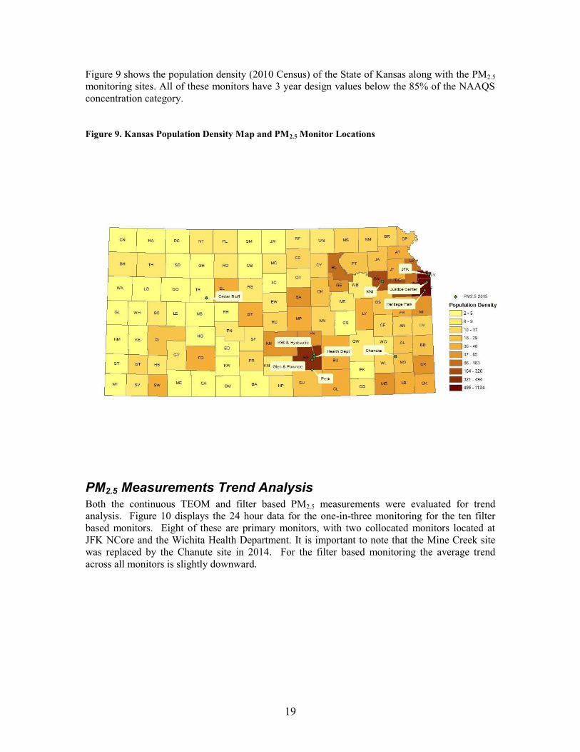
Figure 9 shows the population density (2010 Census) of the State of Kansas along with the PM2.5 monitoring sites. All of these monitors have 3 year design values below the 85% of the NAAQS concentration category. Figure 9. Kansas Population Density Map and PM2.5 Monitor Locations
PM2.5 Measurements Trend Analysis Both the continuous TEOM and filter based PM2.5 measurements were evaluated for trend analysis. Figure 10 displays the 24 hour data for the one-in-three monitoring for the ten filter based monitors. Eight of these are primary monitors, with two collocated monitors located at JFK NCore and the Wichita Health Department. It is important to note that the Mine Creek site was replaced by the Chanute site in 2014. For the filter based monitoring the average trend across all monitors is slightly downward.

20
Figure 10. 24-hr Avg. PM2.5 Filter Based Monitoring Data w/ Trendline 2010-2014
0
5
10
15
20
25
30
35
40
45
50
55
1/1
/20
10
3/1
/20
10
5/1
/20
10
7/1
/20
10
9/1
/20
10
11
/1/2
01
0
1/1
/20
11
3/1
/20
11
5/1
/20
11
7/1
/20
11
9/1
/20
11
11
/1/2
01
1
1/1
/20
12
3/1
/20
12
5/1
/20
12
7/1
/20
12
9/1
/20
12
11
/1/2
01
2
1/1
/20
13
3/1
/20
13
5/1
/20
13
7/1
/20
13
9/1
/20
13
11
/1/2
01
3
1/1
/20
14
3/1
/20
14
5/1
/20
14
7/1
/20
14
9/1
/20
14
11
/1/2
01
4
µg/m
3
Date
Chanute PM25FP Glen & Pawnee PM25FP Health Dept. Wichita PM25FD Health Dept. Wichita PM25FP
Heritage Park PM25FP Justice Center PM 2.5 PM25FP K96 & Hydraulic PM25FP KC Ncore PM25FD
KC Ncore PM25FP KNI Topeka PM25FP Mine Creek PM25FP Peck-Sumner County PM25FP
Average Linear (Average) For the continuous data the trend over the 5-year period, 2010-2014, has also been slightly downward. Figure 11 shows the 24-hour average of the two continuous monitors along with the linear trendline. JFK Center and NCore are the same site location but a 1405DF instrument replaced the existing continuous monitor in 2013. These two continuous monitors are located in opposite ends of the state and one (JFK/NCore) is located in an urban area while the other (Cedar Bluff) is located in a rural area of western Kansas. The JFK/NCore monitor is located in the Kansas City urban area and raises the overall average because it has slightly higher readings on average than the other monitor. Overall, the average continuous and filterable PM2.5 readings across the state are below the NAAQS standard.

21
Figure 11. 24-hr Avg. PM2.5 Continuous Monitoring Data w/ Trendline 2010-2014
0
10
20
30
40
50
60
70
80
90
100
110
120
130
140
150
160
170
180
190
200
210
220
230
240
250
1/1
/20
10
3/1
/20
10
5/1
/20
10
7/1
/20
10
9/1
/20
10
11
/1/2
01
0
1/1
/20
11
3/1
/20
11
5/1
/20
11
7/1
/20
11
9/1
/20
11
11
/1/2
01
1
1/1
/20
12
3/1
/20
12
5/1
/20
12
7/1
/20
12
9/1
/20
12
11
/1/2
01
2
1/1
/20
13
3/1
/20
13
5/1
/20
13
7/1
/20
13
9/1
/20
13
11
/1/2
01
3
1/1
/20
14
3/1
/20
14
5/1
/20
14
7/1
/20
14
9/1
/20
14
11
/1/2
01
4
µg/m
3
DATE
Cedar Bluff JFK Center NCore Average Linear (Average)
Very similar trends are seen when looking at the annual averages. Figure 12 provides the annual average filter based PM2.5 readings from 2002 – 2014. As is seen in the 24-hr case, the trend is slightly downward.

22
Figure 12. Annual Avg. Filter Based PM2.5 Monitoring Data 2002-2014
6.0
8.0
10.0
12.0
14.0
16.0
18.0
2002 2003 2004 2005 2006 2007 2008 2009 2010 2011 2012 2013 2014
µg/m
3PM2.5 Annual Means
Wichita Health Dept. Peck Chanute JFK/KCK JC/KC KNI/Topeka
Annual Standard = 12.0 ug/m3
The design values for each PM2.5 monitor have been listed in Tables 8 and 9. There are no values exceeding the current NAAQS for PM2.5 annual or 24-hour standards. All federal reference monitors are also below 85% NAAQS threshold used for determining minimum monitoring requirements. The TEOM monitors are listed in Italic in Tables 7 and 8 below. Table 7. 24-hr PM2.5 Design Values (98th percentile) - Kansas Monitors (µg/m3)
Site Name 12-14 Average
Heritage Park 16 Cedar Bluff (TEOM,1405-DF) 15
Wichita Health Dept. 22 Pawnee & Glenn 23 K96 & Hydraulic 24 Topeka KNI 20 Peck 21 Kansas City JFK/NCore (TEOM-FDMS,1405-DF)
26
Kansas City JFK 20 Justice Center 17

23
Table 8. Annual PM2.5 Design Values for all Kansas Monitors (µg/m3)
Site Name 12-14 Average
Heritage Park 7.2 Cedar Bluff (TEOM,1405-DF) 7.1
Wichita Health Dept. 8.7 Pawnee & Glenn 9.4 Topeka KNI 8.5 Peck 8.1 Kansas City JFK/NCore (TEOM-FDMS,1405-DF)
**
Kansas City JFK 9.3 Justice Center 7.9 K96 & Hydraulic 8.9 **- Data Not Available for Calculation
Correlations between Kansas PM2.5 Monitors Figure 13 presents the correlation matrix produced from the LADCO NetAssess analysis tool (http://ladco.github.io/NetAssessApp/index.html) for January 1, 2011 through December 31, 2013 PM2.5 measurements. The Correlation Matrix tool generates a graphical display that summarizes the correlation, relative difference and distance between pairs of monitoring sites. Within the graphical display, the shape of the ellipses represents the Pearson correlation between sites. Circles represent zero correlation and straight diagonal lines represent a perfect correlation. The correlation between two sites quantitatively describes the degree of relatedness between the measurements made at two sites. That relatedness could be caused by various influences including a common source affecting both sites to pollutant transport caused meteorology.

24
Figure 13. Correlation Matrix for 2011-13 PM2.5 Measurements in Kansas
Good correlations were observed for the Kansas City monitoring sites. Among the three monitoring sites in Kansas City on the Kansas side all these sites showed a >0.7 R2 correlation and low relative difference. These three sites are also fairly well correlated with the Kansas City, Missouri monitors. All four of the Wichita sites also show very high (> 0.8 R2) correlation among each other. All four sites are located within 25 miles of each other. Note that not all monitors are included in the correlation tool based on data availability. Based on the correlation and the relative close distance between all sites it seems feasible that one of the Wichita PM2.5 sites could be removed. Topeka/KNI is an urban site not too far away (50 miles west) from the Kansas City urban center sites; this site does not show a correlation with the three Kansas City sites. The remaining sites are also further distances from the urban core and generally are not correlated because of the large distances between locations. Even though the correlations are low, most of these sites have similar low design values all below the NAAQS for both the annual and 24-hour standard.
PM2.5 Removal Bias Analysis The NetAssess removal bias tool is meant to aid in determining redundant sites. The bias estimation uses the nearest neighbors to each site to estimate the concentration at the location of the site if the site had never existed. This is done using the Voronoi Neighborhood Averaging algorithm with inverse distance squared weighting. The squared distance allows for higher weighting on concentrations at sites located closer to the site being examined. The bias was

25
calculated for each day at each site by taking the difference between the predicted value from the interpolation and the measured concentration. A positive average bias would mean that if the site being examined was removed, the neighboring sites would indicate that the estimated concentration would be larger than the measured concentration. Likewise, a negative average bias would suggest that the estimated concentration at the location of the site is smaller than the actual measured concentration. So, those sites with large positive bias are more likely candidates to be removed or relocated because they are not measuring the peak PM2.5 in the area. Figure 14 shows the results of this removal bias tool run for PM2.5 sites in Kansas. Red circles indicate positive bias while blue indicate negative bias. Figure 14. PM2.5 Removal Bias Map
Proposed Kansas PM2.5 Monitoring Network 2015-2020 After a careful review of all the above factors, the proposed Kansas PM2.5 monitoring network for the upcoming 5 years is presented in Figure 15. This proposal reflects the population based monitoring requirements along with the current PM2.5 monitored values. Overall, KDHE proposes to install continuous PM2.5 monitors at Heritage Park and Topeka KNI. This will supplement the two current continuous monitors located at Cedar Bluff and the NCore site in Kansas City. In addition, a continuous 1405-DF monitor will be installed at the Wichita Health Department site in the next several years. KDHE will also examine the possibility of removing one PM2.5 monitor in the Wichita area and one of the three monitors in Kansas City. KDHE will continue to make efforts, as funds allow, to replace filter based PM2.5 monitors with continuous monitors across the network.

26
Figure 15. Proposed PM2.5 Monitoring Network 2015-2020
PM10 Monitoring Network
Current PM10 Standard and Monitoring Requirements Current national ambient air quality standards (NAAQS) for PM10 has been set to 150 micrograms per meter cubed for both the primary standard and the secondary standard (http://www.epa.gov/ttn/naaqs/standards/pm/data/fr20061017.pdf). This standard is not to be exceeded more than once per year on average over 3 years. Current minimum monitoring requirements for PM10 are shown in Table 9 (http://edocket.access.gpo.gov/2006/pdf/06-8478.pdf). Table 9. PM10 Minimum Monitoring Requirements (Number of Stations per MSA) 1
Population Category
High Concentration2
Medium Concentration3
Low Concentration4
> 1,000,000 6 - 10 4 - 8 2 - 4 500,000 - 1,000,000 4 - 8 2 - 4 1 - 2
250,000 - 500,000 3 - 4 1 - 2 0 - 1 100,000 - 250,000 1 -2 0 - 1 0
1 Selection of urban areas and actual numbers of stations per area within the ranges shown in this table will be jointly determined by EPA and the State Agency. 2 High concentration areas are those for which ambient PM10 data show ambient concentrations exceeding the PM10 NAAQS by 20% or more. 3 Medium concentration areas are those for which ambient PM10 data show ambient concentrations exceeding 80% of the PM10 NAAQS. 4 Low concentration areas are those for which ambient PM10 data show ambient concentrations < 80% of the PM10 NAAQS.

27
5 These minimum monitoring requirements apply in the absence of a design value. Applying the minimum monitoring requirements to Kansas urban areas, population totals and historical PM10 measurements results in the design requirements are shown in Table 10. According to Tables 9 and 10, PM10 monitors could be removed from the Wichita area and the Kansas City area assuming the Missouri side of Kansas City retains a PM10 monitor. Table 10. Minimum Number of PM10 Monitors Required in Kansas MSA
MSA Population
(2014) Number of Existing
PM10 Monitors PM10 Monitors
Required Wichita, KS 641,076 3 1-2 Topeka, KS 233,758 1 0-1 Lawrence, KS 116,585 0 0 St. Joseph, MO-KS 127,431 0 0 Manhattan, KS 98,091 0 0 Kansas City, MO-KS 2,071,133 2 (KS side only) 2-4
State of Kansas Current PM10 Monitoring Network Current Kansas PM10 monitoring network includes 10 monitors located throughout the state at 8 monitoring sites. Three of the monitors are filter based while the remaining seven monitors are continuous. Monitor locations and type are listed in Table 11 along with detailed site information. One site at JFK/NCORE, has collocated filterable and continuous PM10 measurements. Table 11. State of Kansas PM10 Monitor Site ID and Location
Site Name Site ID City Address Lat_DD Lon_DD Filter PM10
Cont. PM10
Dodge City 057 - 0002 Dodge City
Dodge City Community College 37.77527 -100.035 NO YES
Glen & Pawnee 173 - 0009 Wichita Fire Sta#12 Glen & Pawnee 37.651111 -97.362222 NO YES
Health Dept. 173 - 0010 Wichita Health Dept., 1900 East 9th St. 37.701111 -97.313889 NO YES
Chanute 133 - 0002 Chanute 1500 West Seventh 37.676111 -95.474444 NO YES
Goodland 181 - 0001 Goodland City Fire Sta , 1010 Center 39.348333 -101.713056 YES NO
JFK 209 - 0021 Kansas City
1210 N. 10th St., JFK Recreation Center 39.1175 -94.635556 YES+Colo YES
K-96 And Hydraulic 173 - 1012 Wichita
K-96 And Hydraulic 37.747222 -97.316389 NO YES
KNI 177 - 0013 Topeka 2501 Randolph Avenue 39.02427 -95.71128 NO YES

28
Figure 16 shows the population density of the State of Kansas along with the monitoring sites. All of these monitors have 3 year design values in the Low (< 80% of the NAAQS) concentration category. Figure 16. Kansas Population Density Map and PM10 Monitor Locations
PM10 Measurements Trend Analysis Both the continuous TEOM and filter based PM10 measurements were evaluated for trend analysis. For the continuous data the trend over the 5-year period, 2010-2014, has been slightly downward. Figure 17 shows the daily average of the eight continuous monitors along with the linear trendline. Overall, the average continuous readings across the state are well below the NAAQS standard. The two days of exceedances (Oct. 2012 & April 2014) were caused by dust storms and exceptional event requests letters have been submitted to EPA Region 7.

29
Figure 17. 24-hr Avg. of PM10 Continuous Monitoring Data w/ Trendline 2010-2014
0
20
40
60
80
100
120
140
160
180
200
1/1
/20
10
3/1
/20
10
5/1
/20
10
7/1
/20
10
9/1
/20
10
11
/1/2
01
0
1/1
/20
11
3/1
/20
11
5/1
/20
11
7/1
/20
11
9/1
/20
11
11
/1/2
01
1
1/1
/20
12
3/1
/20
12
5/1
/20
12
7/1
/20
12
9/1
/20
12
11
/1/2
01
2
1/1
/20
13
3/1
/20
13
5/1
/20
13
7/1
/20
13
9/1
/20
13
11
/1/2
01
3
1/1
/20
14
3/1
/20
14
5/1
/20
14
7/1
/20
14
9/1
/20
14
11
/1/2
01
4
µg/m
3
DATE
Chanute Dodge City Glen & Pawnee GWashington&Skinner Health Dept. Wichita
K96 & Hydraulic KC Ncore KNI Topeka Average Linear (Average) Looking at the filter based one-in-six data, a slight downward trend was also apparent like the continuous data. Figure 18 shows the PM10 filter based monitoring data for PM10 sites in the state. Note the higher readings that occurred in 2011 and 2013. These two exceedances were located at the Goodland monitor and were both caused by dust storms associated with strong low pressure systems. Both of these days have been flagged and exceptional event requests were sent to EPA Region 7. EPA has concurred on the Goodland 2011 event. The important point is both the continuous and filter based monitors are all well below the standard. The 420 Kansas monitoring site in Kansas City, Kansas was removed at the end of the 2013. Figure 18. 24-hr Avg. Filter Based PM10 Monitoring Data w/ Trendline 2010-2014
0
20
40
60
80
100
120
140
160
180
1/1
/20
10
3/1
/20
10
5/1
/20
10
7/1
/20
10
9/1
/20
10
11
/1/2
01
0
1/1
/20
11
3/1
/20
11
5/1
/20
11
7/1
/20
11
9/1
/20
11
11
/1/2
01
1
1/1
/20
12
3/1
/20
12
5/1
/20
12
7/1
/20
12
9/1
/20
12
11
/1/2
01
2
1/1
/20
13
3/1
/20
13
5/1
/20
13
7/1
/20
13
9/1
/20
13
11
/1/2
01
3
1/1
/20
14
3/1
/20
14
5/1
/20
14
7/1
/20
14
9/1
/20
14
11
/1/2
01
4
µg/m
3
DATE
Goodland 420 Kansas JFK Primary JFK Collocated Average Linear (Average)

30
The design values for each of the PM10 monitors have been listed in Table 12. There are no values exceeding the current NAAQS. The Goodland monitor has the highest design value reading of 99 µg/m3, is well below the 150 µg/m3 standard. This monitor has been affected by several dust storms during this period which has increased its design value significantly. Several monitors do not have three years of data and no design values are provided for those monitors. Table 12. PM10 Design Values for all Kansas Monitors (µg/m3)
Site Name 2012 2nd High
2013 2nd High
2014 2nd High
12-14 Design Value
Chanute (TEOM) * * 80 ** Goodland 107 136 53 99 KCK JFK 51 44 49 48 KCK NCore * 61 62 ** Dodge City (TEOM) 55 31 62 49 Washington & Skinner (TEOM) 86 36 * **
Glen & Pawnee (TEOM) 95 71 103 90
Wichita Health Dept (TEOM) 86 71 104 87
K96 & Hydraulic (TEOM) 82 85 110 92
Topeka KNI (TEOM) 48 55 62 55 *No data **3 years of data not available for calculation
Proposed Kansas PM10 Monitoring Network 2015-2020 After a careful review of all the above factors, the proposed Kansas PM10 monitoring network for the upcoming 5 years is presented in Figure 19. This proposal reflects the population based monitoring requirements along with the current PM10 monitored values. Overall, KDHE proposes removing the filter based PM10 monitors in Goodland and in Kansas City. KDHE will replace the Goodland filter based monitor with a continuous monitor located at the Cedar Bluff monitoring site. KDHE has installed this monitor and is currently evaluating it against the Goodland monitor. This will leave eight continuous PM10 monitors, one in Dodge City, one at Cedar Bluff, three in Wichita, one in Chanute, one in Topeka and one in Kansas City, KS. KDHE will continue to examine the data from the three existing PM10 monitors in Wichita and decide whether there is a need for all of those sites in the future.

31
Figure 19. Proposed PM10 Monitoring Network 2015-2020
NCore Monitoring Site
National Ambient Air Monitoring Strategy The Environmental Protection Agency (EPA) developed a National Ambient Air Monitoring Strategy (NAAMS). The goal of the strategy is “to improve the scientific and technical competency of existing air monitoring networks to be more responsive to the public, and the scientific and health communities, in a flexible way that accommodates future needs in an optimized resource-constrained environment” (National Ambient Air Monitoring Strategy Document). As part of the Strategy, a network design was proposed called the National Core Network (NCore). This network accommodates the overall strategic goals as well as determines air quality trends, report to the public, assess emission reduction strategy effectiveness, provide data for health assessments and help determine attainment / non-attainment status. NCore introduced a new multi-pollutant monitoring component, and addressed the following major objectives: The NCore monitoring network addresses the following monitoring objectives which are equally valued at each site:
timely reporting of data to the public through AIRNow, air quality forecasting, and other public reporting mechanisms;
support development of emission strategies through air quality model evaluation and other observational methods;
accountability of emission strategy progress through tracking long-term trends of criteria and non-criteria pollutants and their precursors;
compliance through establishing nonattainment/attainment areas by comparison with the NAAQS;

32
support of scientific studies ranging across technological, health, and atmospheric process disciplines; support long-term health assessments that contribute to ongoing reviews of the National Ambient Air Quality Standards (NAAQS); and
support of ecosystem assessments, recognizing that national air quality networks benefit ecosystem assessments and, in turn, benefit from data specifically designed to address ecosystem analysis.
At a minimum, NCore monitoring sites must measure the parameters listed in Table 13. Table 13. NCore Parameters
NCore Site - Urban 20-209-0021; Kansas City: This site (Figs. 20-21), which currently serves as an urban core multi-pollutant monitoring station, is designated as a NCore station. The site is located close to Nebraska Ave and North 10th Street, Kansas City, Kansas (N 39.117219; W -94.635605). Figure 20. Kansas City, KS JFK NCore Site Map

33
Figure 21. Kansas City, KS JFK NCore Site
KDHE does not plan to expand the NCore Monitoring Network in the near future.
Kansas Ambient Air Monitoring Plan for Lead (Pb)
Source-oriented Monitoring According to 40 CFR Part 58, Appendix D, paragraph 4.5(a), state and, where appropriate, local agencies are required to conduct ambient air monitoring for lead (Pb) considering Pb sources that are expected to or have been shown to contribute to a maximum Pb concentration in ambient air in excess of the NAAQS. At a minimum, there must be one source-oriented SLAMS site located to measure the maximum Pb concentration in ambient air resulting from each Pb source that emits one-half (0.5) or more tons per year. A search of reported emissions for 2007 revealed that only one source in Kansas exceeds the one-half ton threshold. This source is located at Salina. According to 40 CFR Part 58, Appendix D, paragraph 4.5(a), source-oriented monitors are to be sited at the location of predicted maximum concentration in ambient air taking into account the potential for population exposure, and logistics. Typically, dispersion modeling will be required to identify the location of predicted maximum concentration. Dispersion modeling was performed by KDHE to determine the area of maximum concentration for sampler placement. KDHE prepared a Monitoring Plan for Airborne Lead in 2009. The Pb site near the Exide Technologies facility at Salina, KS has been designated with AQS site ID 020-169-0004. A high volume (HiVol), total suspended particulate (TSP) sampler is running at the site on a 1/6 day schedule and began sampling on February 2, 2010. KDHE installed an additional high volume (HiVol), total suspended particulate (TSP) sampler at the Salina monitoring site to use for collocation purposes in 2013. This monitor runs on the same 1/6 day sampling schedule as the existing lead monitor and was installed next to the existing monitor. The monitoring site is located at the following legal description: SOUTH INDUSTRIAL AREA, S1, T15, R3, BLOCK 2, ACRES 13.4, LTS 21-30 EXC E 32 LT 30

34
Figure 22. Salina, KS Lead Source Monitoring Site
Figure 23. Salina, KS Lead Source Monitoring Site Map

35
Figure 24. Salina, KS Lead Nonattainment Area Map
Population based Lead Monitoring EPA also requires lead monitoring in large urban areas. These monitors are located along with multi-pollutant ambient monitoring sites (known as the “NCore network”). Lead monitoring at these sites began January 1, 2012. KDHE located a high volume (HiVol), total suspended particulate (TSP) sampler at the JFK NCore site in Kansas City, Kansas to fulfill this requirement. It is running at the site on a 1/6 day schedule and began running December 27, 2011 and took its first sample on January 4, 2012. Because of low values recorded at these NCore based lead monitor sites across the country, EPA has proposed to eliminate this monitoring requirement. As of April 2015, this proposal has not yet become finalized and lead monitoring will continue at this site.
Mercury Deposition Monitoring in Kansas KSA 75-5673 originally required that the Kansas Department of Health and Environment (KDHE) establish a statewide mercury deposition network consisting of at least six monitoring sites. Monitoring for a period of time long enough to determine trends (five or more years) was also specified. Legislative changes were enacted in 2014 that keep a network in place but allow the KDHE to re-examine the network size and location of the original six sites as established in

36
response to KSA 75-5673. KDHE has reconfigured the network to now include four sites across the state. These network changes will continue to assure compatibility with the national Mercury Deposition Network (MDN). The MDN, coordinated through the National Atmospheric Deposition Program (NADP), is designed to study and quantify the atmospheric fate and deposition of mercury. The MDN collects weekly samples of wet deposition (rain and snow) for analysis to determine total mercury. The current Kansas Mercury Wet Deposition Monitoring Network (KMDN) consists of four sites distributed across the state. The locations of existing and future sites in the states of Nebraska and Oklahoma were also taken into consideration to optimize regional mercury network coverage. A more detailed report on this network may be found at http://www.kdheks.gov/bar/air-monitor/mercury/Hg_Report.pdf. A map of the network appears below in Figure 25. Figure 25. Proposed Mercury Wet Deposition Network (incl. recently closed sites) 2015-2020
Sulfur Dioxide Monitoring Network On June 2, 2010, EPA revoked the primary annual and 24-hour SO2 standards from 30 ppb and 140 ppb, respectively, to a 1-hour standard of 75 ppb. The new SO2 rule, published June 22, 2010, also stated the following:
Any new monitors must be in operation by January 1, 2013. Monitoring required in Core Based Statistical Areas (CBSA’s) based

37
on population size and SO2 emissions. Additional monitoring would also be required based on the state’s
contribution to national SO2 emissions, which could be placed either within or outside a CBSA’s.
Reporting requirement added to include maximum 5-minute block average of each hour.
KDHE currently monitors for SO2 at the following sites; Cedar Bluff, Peck (Wichita), Chanute and JFK (Kansas City).
Proposed Kansas Sulfur Dioxide Monitoring Network 2015-2020 KDHE intends to maintain the current configuration of its SO2 network. Figure 26. Proposed Sulfur Dioxide Monitoring Network 2015-2020
Nitrogen Dioxide Monitoring Network The state is required by 40 CFR 58 Appendix D to install and operate one microscale near-road NO2 monitoring station and it is to be operational by January 1, 2017. The state is beginning to perform preliminary analysis on the selection of an appropriate near-road monitoring site in Wichita and will wait funding to establish this site. (EPA is currently discussing the possibility of not proceeding with the implementation of this phase of the NO2 Rule. As of the development of

38
this plan, no final decisions have been made.) EPA amended the applicability requirements of 40 CFR 58 Appendix D in March of 2013 to address the near road monitoring network and introduced a phased approach to implementation of the network. Two criteria have been set up for NO2 monitoring:
Near-road NO2 monitoring; 1 micro-scale site would be required in CBSAs >= 350,000 at a location of expected highest hourly NO2 concentrations sited near a major road with high AADT (Annual Average Daily Traffic) counts.
Community-wide; required in CBSAs >= 1 million at a location of expected highest NO2 concentrations representing neighborhood or larger (urban) spatial scale.
Based on the near-road criteria, one monitor site was installed in 2013 in the Kansas City Metropolitan Area by the Missouri Department of Natural Resources Air Pollution Control Program and is located near I-70 and Sterling Avenue (39.047911, -94.450513, Figures 27-28). Based on the community-wide criteria, the Kansas City CBSA would be required to have a monitor and the JFK NCore monitoring site (20-209-0021) satisfies this requirement. Figure 27. Kansas City (MO.) Near-Road Nitrogen Dioxide Monitoring Site, 2015

39
Figure 28. Kansas City (MO.) Near-Road Nitrogen Dioxide Mon. Site Map, 2015
Proposed Kansas Nitrogen Dioxide Monitoring Network 2015-2020 KDHE intends to maintain the current configuration of its NO2 network. Figure 29. Proposed Nitrogen Dioxide Monitoring Network 2015-2020

40
Carbon Monoxide EPA conducted a review of the CO NAAQS and decided to retain the existing standards in 2011. The BOA currently has one CO monitoring site in the state (Figure 30). It is located at the JFK NCore site in Kansas City, KS.
Proposed Kansas Carbon Monoxide Monitoring Network 2015-2020 KDHE intends to maintain the current configuration of its CO network. Figure 30. 2015 Carbon Monoxide Monitoring Network


