Eotvos Lorand UniversityFaculty of Science

Katalin Papp

An Artificial Neural Network:the Support Vector Machine

BSc Thesis

Supervisor: Gabriella KeszthelyiDepartment of Analysis

Acknowledgments

I would like to thank my supervisor, Gabriella Keszthelyi, for introducing meto this intriguing topic, and guiding me steadily through both good times andbad. She has shown me how analysis holds more beauty than it lets on at firstglance, and never let me lose faith in our work together.

I am also grateful for the support of my mother and my friends, and myfellow students at ELTE. They made these years truly worth it.

Contents

1 Introduction 11.1 A different point of view . . . . . . . . . . . . . . . . . . . . . . . 1

1.1.1 What measure is an intelligent machine? . . . . . . . . . . 11.1.2 Neurobiological inspirations . . . . . . . . . . . . . . . . . 2

1.2 A brief history of artificial neural networks . . . . . . . . . . . . 3

2 Artificial Neural Networks 52.1 Structure and function . . . . . . . . . . . . . . . . . . . . . . . . 5

2.1.1 How to build an artificial brain . . . . . . . . . . . . . . . 52.1.2 Trial and error: teaching our machine . . . . . . . . . . . 7

2.2 Basic feedforward networks . . . . . . . . . . . . . . . . . . . . . 112.2.1 Perceptron and Adaline . . . . . . . . . . . . . . . . . . . 112.2.2 Multilayer perceptron and the backpropagation algorithm 132.2.3 Radial basis function networks . . . . . . . . . . . . . . . 16

3 Support Vector Machines 173.1 Linear SVM . . . . . . . . . . . . . . . . . . . . . . . . . . . . . . 18

3.1.1 The linearly separable case . . . . . . . . . . . . . . . . . 183.1.2 Soft margin: the linearly mostly separable case . . . . . . 23

3.2 Nonlinear SVM . . . . . . . . . . . . . . . . . . . . . . . . . . . . 243.2.1 Feature map: transforming the problem . . . . . . . . . . 243.2.2 Kernel trick . . . . . . . . . . . . . . . . . . . . . . . . . . 25

4 Implementations & Applications 284.1 Implementations . . . . . . . . . . . . . . . . . . . . . . . . . . . 28

4.1.1 ANN Software . . . . . . . . . . . . . . . . . . . . . . . . 284.1.2 Hardware implementations . . . . . . . . . . . . . . . . . 28

4.2 Applications . . . . . . . . . . . . . . . . . . . . . . . . . . . . . . 294.2.1 Traditional and modern uses . . . . . . . . . . . . . . . . 294.2.2 Interpreting the model . . . . . . . . . . . . . . . . . . . . 31

4.3 A conclusion . . . . . . . . . . . . . . . . . . . . . . . . . . . . . 31

1 Introduction

1.1 A different point of view

1.1.1 What measure is an intelligent machine?

In the XX. century, with the introduction of computers with a high comput-ing capacity, lots of previously unsolvable problems got feasible solutions. Manycenturies worth of mathematicians’ work came to fruition: with a machine to cal-culate millions of operations in the nick of time, numerical methods are thriving.The general approach is as follows: identify the problem, devise an algorithmwith realistic run-time, and let the computer do the dirty work.

The question follows naturally: what if we can not come up with an efficientalgorithm, or, worse, with any sensible algorithm at all? For example: we needa program that can read handwriting and can quickly digitalize the sentenceswritten by the user. How do we tell the machine what the letter ”A” looks like,if every person writes it differently? Why can’t a machine solve a task than anyeight-year-old can?

Figure 1: A set of handwritten digits. A neural network trained to recognizethem can be found at [1].

The problem lies in the difference between how humans and computers solveproblems. The latter view everything as data, while the former view everythingas patterns. Humans have difficulty memorizing data that does not ”makesense” such as telephone numbers, or dozens of dates for a History test. Itshouldn’t come as a surprise that many learning techniques for students consistof making up some artificial relations between bits of information. Computers,on the contrary, can store, sort, or summarize without much effort, but they lagbehind when it comes to classic AI problems: speech and handwriting recogni-tion, and vision. [2]

The issue is a bit more general: we do not know nearly enough about how ourbrains work, how information is stored, organized and recalled, and this leavesus helpless in the face of teaching a computer to complete the aforementionedtasks. That aside, we are not completely unarmed: what neuroscience gave usis the concept of artificial neural networks (ANN).

1

Figure 2: A biological neuron and its mathematical representation [3]

1.1.2 Neurobiological inspirations

Animals and humans interact with the world through their nervous systems,which consists of cells called neurons. They are star-shaped with a long tailcalled axon, and they function by transmitting signals to one another, creatingcomplex systems capable of guiding our senses, controlling our body and pro-cessing information. Our central nervous system, which lets us think and solveproblems, is located in our spine and our head. (Through decades of research),neuroscientists have managed to find correlations between certain parts of thebrain and their activity. The patterns in which the neurons are interconnectedare probably responsible for our memories, but there are lots of theories on thesubject.

A neuron receives signals from the ones connected to it through gates calledsynapses, and these signals either excite or inhibit its activity, and if the col-lected signals reach a certain threshold, the neuron sends an electrochemicalpulse called action potential through its axon, alerting other cells.

The nervous system’s adaptiveness and its ability to learn gave rise to theconcept of ANNs. The basic premise is that instead of a huge, linear algorithmicsolution, we could use many parallel ”cells” arranged in layers, that each eval-uate their input and send it the ones connected to it, with a decision functionat the end to combine them.

The most interesting feature of these networks is their ability to learn. Ahuman infant is equipped with millions of neurons when she is born, all readyto grow connections with each other to let her understand the world. If wecould arm our computers with the same ability, they could solve unimaginableproblems.

2

Figure 3: Frank Rosenblatt with the image sensor of the Mark I Perceptron [4]

1.2 A brief history of artificial neural networks

As early as 1943, Warren McCulloch and Walter Pitts, a neurophysiologist anda logician came up with a computational model that consisted of neurons, whichthey believed to be the base logic units of the brain. McCulloch and his teamexamined the structure of the frog’s visual system, and the way it not onlytransmitted, but organized information.

Alan Turing has proposed the idea as early as 1948, under the name ’un-organized machines’. He thought of the neural model as the simplest way toimitate a child’s learning.

In 1949, psychologist Donald O. Hebb sought to understand the brain’s learn-ing process, and he proposed a theory that became known as ’Hebbian learning’.His premise is as follows: if two neurons often fire at similar moments, in re-sponse to similar stimuli, their connection becomes stronger. A catchy phrasingof this theory is ”neurons that fire together, wire together”.

The first researcher to actually endeavor to build a neural machine wasNathanial Rochester, working at the IBM laboratories in the 50s. These at-tempts failed, at first, but similar efforts have succeeded afterwards, for exampleB. G. Fairley’s and Wesley A. Clark’s Hebbian network at MIT.

In 1956, at the famous Darthmouth Summer Conference, which becameknown as the inception of modern artificial intelligence research, neural networkswere a prominent topic, among language processing and many other classic AIproblems.

Frank Rosenblatt built the perceptron in 1960 at the Cornell AeronauticalLaboratory in Buffalo. Inspired by the eye of the fly, it was capable of binary

3

classification in linearly seperable cases.In the same year, at Stanford University Bernard Widrow and Ted Hoff builtthe adaline, a linear network with similar abilites. They have also proposeda multi-layer network called madaline, but without backpropagation, they re-sorted to less effective learning algorithms.

All of this early success, and the general hype led to expectations that themachines of the era could not live up to. Traditional von Neumann modelsproved more useful, and neural reasearchers lost both interest and funding.In 1969, Marvin Minsky and Seymour Papert wrote Perceptrons, an infamousbook known for diminishing the last grains of belief in neural networks. In thiswork, they’ve proved that the XOR function couldn’t be learned by a single-layer machine, as it is linearly non-separable. They have left the chance formulti-layer networks to succeed in this simple task, but their book was heavilymisinterpreted, and neural research halted for almost two decades.

The renewed interest in the field in the 80s could be attributed to numerousfactors: the discovery of the backpropagation method and thus the advent ofgenerally applicable networks such as the multi-layer perceptron, the competi-tion with Japanese researchers, and increased computational power.Another decline in popularity came in the 90s through the early 00s, as simplermodels such as the support vector machine were found to be more effective,easier to inperpret, and computationally more feasible.

Nowadays neural networks live their third renessaince, under the umbrellaname deep learning. Deep neural networks are multi-layer networks in whichthe layers act very differently. They are believed to circumvent the classic datamining step of feature extraction, a method which is more art than science.Instead, these machines are fed extreme amounts of raw data, and left alone tofigure out the rest themselves.Of course, the success of these systems higly depends on the underlying hard-ware, as they consume massive computing resources. Contemporary networksuse GPUs, as they are built to handle the vast amounts of matrix and vectorcalculations demanded by the deep learning algorithms.Another area of recent interest are the so-called recurrent neural networks, whichpossess their own sort of internal memory, for example the long-short term mem-ory (LSTM) machine.

These modern networks, and hybrid solutions using them perform best inpattern recognition problems such as handwriting, traffic light and voice recogni-tion, and they find their uses in numerous other fields, such as biology, medicine,or financial forecasting.This is a rapidly developing field, with many unanswered questions and mys-teries to explore, and learning machines may play a very important part in thefuture of computing in general.

4

2 Artificial Neural Networks

2.1 Structure and function

2.1.1 How to build an artificial brain

While there is no single definition of what an ANN is, it can be defined as aparallel information processing machine with the following characteristics:

1. An ANN is composed of mostly uniform processing units called neurons,which are connected according to a previously defined order.

2. An ANN approximates a non-linear function of its input vector.

3. An ANN is capable of learning by tuning a set of adaptive weights, andthis process is defined by a learning algorithm.

There are two stages of life that all ANNs go through: the learning phase,and the recall phase.

In the learning phase, of which one may think as the ANN’s childhood, itis fed the learning set, a set of data we usually have some information about.During this stage the ANN sets its weights using its learning algorithm. This isoften a slow and memory-consuming process.After fine-tuning itself on the learning set, the recall phase begins, in which ituses the knowledge it learnt to solve the actual problem, now working fast andefficiently. It should be noted that these stages are often mixed, as the ANNcan continue its learning. When its environment changes over time, it is able toreevaluate itself over and over again.

There are three different learning methods in use: supervised, unsupervised,and reinforcement learning. The first one, also called ’learning with a teacher’is the one we will discuss in detail in the following chapters, as all of ANNsdescribed here use it. Supervised learning means we, the ’teachers’ are smarterthan the machine: for example, this is the case in image recognition. We knowvery well which of the pictures depict people and which do not. The untrainedmachine makes guesses, and after each guess, we tell it if it was right, and itlearns - modifies its weights - based on our answers.Unsupervised learning, or ’learning without a teacher’ means we are just asbefuddled with the input as the machine. We have little idea what kind of re-sult do we expect. This is the case in data mining and statistics: the machineshould look for patterns in enormous amounts of data, or preprocess it some-how to make it more digestible for other methods. This involves clustering theinformation, or rooting out redundancies in large databases.Reinforcement learning differs greatly from the previous ones as there is noready-made data set to learn from. The machine is placed in an environmentand offered some courses of action instead; think of a mouse in a labyrinth.After performing an action, it experiences a reaction from the world around it,and weights its choice depending on the reaction. In this case, we expect themachine to optimize its own behavior in the selected environment, for example,it should learn to control a robot, or play a game effectively.

5

An ANN is composed of processing units called neurons, arranged in oneor more layers, which are sorted into one of three categories: the input layer,the output layer, and the hidden layer(s). There can be as many of theseas convenient, but there should be at least one input layer, since it mostlyjust serves as a buffer for the information the ANN receives, performing somesimple linear function. Maybe the easiest way to visualize the ANN’s structureis as a digraph, with the neurons as nodes and the directed edges denoting theinterconnections between them. If the resulting graph is a Directed AcyclicGraph (DAG), then we are looking at a feedforward network. Otherwise it iscalled a recurrent network.I will examine the following structures in detail:

1. the most basic single-layer networks (the perceptron and the adaline)

2. the multilayer perceptron (MLP)

3. the radial basis function (RBF) network

4. and, of course the support vector machine (SVM).

While there are numerous other models in use, those are beyond the limitsof this paper.

The ANN’s capabilities highly depend on its structure, on its complexity.The simplest ANN model, composed of a single neuron, calculates a non-linearfunction of the input vector x, taken from the input space X, which is usuallysome subset of Rn, by first multiplying it with their weight vector w ∈ Rn, andthen feeding the product to their decision function f : R→ R. The latter, some-times called the activation function is a monotonically increasing function. Asimple slope or a non-continuous function like the Heaviside function can serveas a decision function, but in later example we will mostly use continuous sig-moid functions such as the hyperbolic tangent and the logistic function, becausein multilayer networks their easily computable derivatives make them more con-venient. If we refer to the elements of the input vector as x = {x0, x1, ..., xn},and to the elements of the weight vector as w = {w0, w1, ..., wn}, then theanswer a neuron gives us is as follows:

y = f(wTx) = f(

n∑i=0

wixi)

Usually the actual input only begins from the first index, and w0 is used tochange the activation function’s threshold, with x0 as constant 1.In this form, an ANN can be viewed as a non-linear function f(w,x), whosevalues depend on both the parameter and the input, so it is really only an ele-ment of a function class defined by its parameter. As we will see in the followingchapter, its learning simply means finding an optimal parameter w*.But let us not forget that choosing the function class and the number of theparameters is up to us, too, and this is what we will refer to as the machine’scomplexity: the size of the function class to choose from, the size of the vectorw. This correlates to the structure of the ANN, but their exact relationship,and the methodology of choosing a function class with ideal complexity is notat all trivial.

6

2.1.2 Trial and error: teaching our machine

As I have mentioned before, in this paper we will take a closer look on thesupervised learning model. This means that for each input vector xi, we havea desired response di, so the training set consists of pairs of (xi, di). In classifi-cation problems, when we are expecting a yes-or-no answer, di has a value of 0or 1. We want the machine to give a correct answer to as much of the xi inputsas possible, or, in other words, to minimize the following:

ε =

m∑i=1

yi − di

,granted that we have m elements in the training set.

Since the machine’s answers and thus its error is defined by the parameter w,we should include w in the function to be minimized. This is called the lossfunction, or the cost function L(d, f(x,w)), which can be chosen according tothe task at hand. In classification problems, for a (x, d) element of the trainingset it is simply 1 or 0 depending on whether d = f(x,w) or not. In regressionproblems it means some kind of distance between d and f(x,w), for examplethe square of their difference:

L(d, f(x,w)) = (d(x)− f(x,w))2

The empirical risk is the mean of the machine’s errors on the training set,

Remp(w) =1

m

m∑i=1

L(di, f(xi,w)).

If the loss function is continuous and differentiable, then finding its minimumin w is equal to looking for the global minimum point of a function of manyvariables, w*, which is a formidable problem on its own. If we set the inputvector x as a constant, the loss function defines an n-dimensional surface on theparameter space. In case this surface has a convenient shape, for example itis convex, or better, quadratic, then the local minimum is easily approximablewith gradient-based numerical methods. The basic premise is calculating theloss function’s gradient in a starting w, and then going the opposite direction,where the function descends the steepest. We can choose the amount we movein each step arbitrarily, thus defining the ”learning speed”.Of course there are smarter ways to do this, for example one of the most popularmethods is the conjugate gradient method. In each iteration of this algorithmwe calculate the best amount to descend in the gradient’s direction, by solvinga one-dimensional minimization problem. There are many variations to thismethod that result in faster convergence on problematic surfaces, like narrowcanyons or banana-shaped trenches.

We are in much deeper trouble if the loss function has local minima. Thereare lots of heuristic methods of avoiding these pits on the loss surface, but inthis case we might try our chances with a so-called stochastic search algorithm.These algorithms wander the parameter space randomly or according to someagenda.

7

Figure 4: The non-linear conjugate gradient method falls into one of the localminima, depending on its starting point. [5]

A popular class of these is called the genetic algorithms. These methods uti-lize another biological phenomenon, the principle of the survival of the fittest.First, some sufficiently diverse elements of the parameter space are chosen, thesevectors are the starting population. Then, using each of them the value ofL(d, f(x,w)) is calculated to evaluate their fitness. Finally, the fittest of themare ”bred”, by mixing some of their coordinates and thus producing offspring,some part of the population is randomly mutated, and the least fit are retired,and the whole process starts again with the new population until an adequatespecimen is produced. The size of the population, the percentages correspond-ing to the amount of breeding and mutations are all chosen arbitrarily, tailoredto the actual problem.Generally, there are as many minimization methods in use as many ANNs, butin any case we should end up with an optimal w*, or at least a sufficient ap-proximation, an we can take comfort in the fact that our network has in factlearnt the training samples.

However, now we encounter a problem inherent in our teaching method: wecan train the machine on the training set as much as we want, but how canwe guarantee that it will perform just as well on unknown inputs? Aside fromthe learning capability, we should introduce a new, desired trait of the ANNs:generalization.Generalization is one of the key elements of human learning. Although onlybeing exposed to a small set of experiences, we are able to react accordinglyto a vast number of events, for example, after being bitten by a stray dog atthe age of 5, we will be cautious with animals of all kinds. Or having tastedapple tea, we are eager to drink other fruit infusions as well. While prejudicescan be both beneficial and harmful, our reliance on them makes assessing newinformation somewhat easier.

Let’s see what we expect from our machines. At this point, it is useful tointroduce the R risk function separately from the empirical risk function, be-

8

Figure 5: Separating all possible colorings of three points on the two-dimensionalplane, and the linearly non-separable XOR problem

cause we can only measure the latter, but would prefer to minimize the former.The risk function is the expected value of the loss function on the unknown prob-ability distribution of the possible inputs, p(w, d), which we hope to estimateby calculating the empirical risk.

R(w) = Ex,d(L(d, f(x,w))),

where the loss function is defined as above.

Generally, supervised learning would be useless if it only meant that themachine can predict information we already know, albeit doing that with ex-treme precision. We would like to assume that by using larger training sets,meaning when m→∞, the Remp → R, but for more certainity, we should turnto Statistical Learning Theory.Russian statisticians Vladimir Vapnik and Alexey Chervonenkis proposed theempirical risk minimization (ERM) principle, defining the conditions of consis-tency, calculating bounds on the risk, and making predictions on the convergencespeed.

They introduced the so-called VC-dimension to measure the complexity oflearning machines, or, as I have mentioned before, the underlying functionclasses. While there are more than one ways to define this number, I willuse the one I have found easiest to understand, one used only for classifyingmachines.A function class’ VC-dimension is h, if there exists an arrangement of h ele-ments of the input space of which each labeling (associating them with 0 or 1,or coloring them black or white) is separable by an element of the function class,but there are no h+1 such elements. For example, if we are using n dimensionalhyperplanes to separate point in a n+ 1 dimensional space, this function class’VC-dimension is n + 1. At the same time, it is not true that we can separateall the colorings of all the n + 1 points in the space, for example, if the pointsare not linearly independent, then there are colorings that can not be linearlyseparated. The definition only demands the existence of one totally separable

9

set of points.There are function classes with ∞ VC-dimension, for example the multi-layerperceptron is one of them. In these cases the following results are mostly useless,but this does not mean that these systems are useless too. It only means thattheir analysis demands a different approach.

The connection of a function class’ complexity and its generalization abilitiesis best illustrated with the example of polynomial interpolation.In interpolation, the complexity is simply the degree of the interpolating poly-nomial. This should match the number of base points (or be less than that, incurve fitting), or else the polynomial is not unique: it can be random outsidethe base points, generating an arbitrarily big error while fitting perfectly on thetraining values.

Vapnik and Chervonenkis calculated the following upper bound on the actualrisk, which holds with a probability of 1− η, called the level of confidence:

R(w) = Remp(w) +ε(h)

2

√1 +

4Remp(w)

ε(h)

and ε(h) denotes

ε(h) = 4h(ln( 2m

h ) + 1)− ln(η4 )

m

This formula shows how the real risk depends on two values: the empiricalrisk, as we expected, but also on the model’s VC-dimension, or, rather, the ratioof the VC-dimension h, and the number of training points, m. As the latterincreases, the upper bound depends more and more on the empirical risk, justas we hoped it would. If the second part is sufficiently low, we can be sure thatthe w* found by the learning algorithm on the surface defined by Remp(w) isclose to the minimum point of the R(w) as well.However, a more complex machine can learn a training set with more precision,producing a lower empirical risk, but its VC-dimension is higher, and it needsmore training points to keep the m

h ratio in balance.

While it seems like using as many training points as possible is the bestsolution to all of these problems, in reality this is not a feasible solution. In realproblems our training sets are finite, and broadening them is costly or otherwiseinadvisable.Vapnik and Chervonenkis suggested a technique called structural risk minimiza-tion (SRM) to find the optimal function class for an actual problem with a giventraining set. It involves using more and more complex systems to solve the sameproblem, with monotonously increasing VC-dimensions, and in each step calcu-lating both parts of the upper bound, looking for the ideal function class. Thebound will first decrease, as the system becomes capable of learning the trainingset, but after a point it will start increasing, at which point we should stop, anduse the system with the lowest bound.

This is a fine idea, but in most cases determining the VC-dimension of afunction class is very difficult, and we only have rough estimates.

10

Another problem is that this upper bound is not very tight either, the actualperformance of a machine can be considerably better. This is especially truein case of models with an infinite VC-dimension, where this upper bound ismeaningless.

Still, the SRM method is a good idea, and its founders formulated the Sup-port Vector Machine in accordance to it. Its whole purpose is lowering bothparts of the bound simultaneously, as we will see in the next chapter.

All in all, choosing the right model, and the best number of parametersand neurons is just as interesting a problem as choosing the exact parameters.This is usually an empirical process, and it involves trying many different meth-ods until we find an appropriate one for the problem at hand. Let’s finish thistopic with a few useful tips on how to make do with a finite set of training points.

For the reasons described above, the value of the empirical risk in its mini-mal point is not very reliable in itself. To measure the machine’s abilities moreprecisely, we should separate a subset of the training set, and create a so-calledvalidation set. Then we teach the network on the remaining points, and thentest it against the validation set’s points, thus getting a more realistic pictureabout how well it would perform on unknown input.For an even more thorough examination, we could divide the training set into ksmall sets, and teach it using k− 1 sets, then test it on the remaining one; thenrepeat the whole process leaving out another small set. This method is calledcross-validation. If the training set’s size is extremely limited, we could leaveonly one point out in each iteration. Of course, this means going through thewhole training process k times, which may take lots of time.

This method could also be applied when we need to compare algorithms im-partially. According to the ”no free lunch” principle, in machine learning thereis no single solution that works in all of the cases; the problems we are tryingto solve are too diverse. One model may triumph victoriously over another inone field, and lag behind embarrassingly in another. Universal solutions aretrumped by specialized ones. Therefore, if we encounter a new problem, thebest we can do is try, fail and learn ourselves, too.

2.2 Basic feedforward networks

2.2.1 Perceptron and Adaline

The two networks I present in this section, Frank Rosenblatt’s perceptron andBernard Widrow’s adaline (adaptive linear neuron) have been invented inde-pendently, only a few years apart. Both function as classifiers, so if we dividethe learning set X into subsets X1 and X2, these machines will learn how todistinguish the training vectors belonging to each, and they are capable of sort-ing new, unknown input vectors into their respective categories as well. Thisproblem could also be formulated as a yes-or-no question, where one subset rep-resents the inputs for which the answer is positive, and the other as the inputswhere the answer is negative.

11

While they are very similar in their structure, their learning algorithms arevery different, giving them different abilities. They both look like the simplenetwork I’ve defined in the previous chapter, calculating a weighted sum of theinput vectors’ elements, and they both use the step function as their decisionfunction.

Figure 6: The perceptron gives its answer y by calculating a weighted sum ofthe input vector, and then feeding it to a step function

Rosenblatt’s perceptron, invented in 1956, is a simple linear classifier. Itgives yes-or-no answers by calculating a weighted sum of the input vector, wTx,and then checking whether it is positive or negative with its decision function f .Its learning algorithm looks for a hyperplane in the n-dimensional input spacethat separates the vectors of the two subsets, or rather the normal vector of onesuch hyperplane. This w* vector is usually not unique, and, if the classes arenot linearly separable, may not even exist.The latter is a serious drawback of the perceptron model. The good news is,however, that there is concrete proof that the learning algorithm I will describealways finds a sufficient hyperplane in a finite amount of steps, and with a con-vergence speed only affected by the dimensionality of the input.

The learning algorithm is as follows: in the k-th learning step, we changethe weight vector according to

w(k+1) = w(k) + αε(k)x(k),

where ε(k) is the classification error and α is the learning rate, a positivevalue, usually between 0 and 1. This learning algorithm is as simple as it gets:if the perceptron got the answer right, then w remains unchanged, if it made amistake, then w is altered by a signed amount of the misclassified vector.The teaching must go on until all the training vectors are learned, and whilethe algorithm may need to process the whole training set repeatedly to get itright, it will eventually find an optimal w*.

The adaline, conceived in 1959, while similar in structure, learns very dif-ferently. While it also has a step function as a decision function, it evaluatesits error and corrects itself according to the weighted sum wTx instead of ayes-or-no answer. It minimizes a cost function which is the mean of the squarederrors:

12

C(w) =1

m(

m∑j=0

dkj −wTxj)

Minimizing this function is relatively easy, since it is equal to solving a sys-tem of linear equations.

The adaline is not limited to linearly separable cases, it finds the optimalw* that minimizes the error. However, the cost function’s value in its minimumpoint may be greater than zero, and this means the machine can not learn everytraining set perfectly.

There are many variations to these simple networks, for example the trainingrate in the perceptron can be defined as a function of k, this way the algorithmcould take smaller steps as it processes the training set again and again.While these networks, especially modern versions of the perceptron are still inuse, their applicability is very limited. Most of their limitations can be negatedwith introducing more layers, as it is seen in the next part. Of course, thisincrease in complexity creates new problems in itself.

2.2.2 Multilayer perceptron and the backpropagation algorithm

The multilayer perceptron’s (MLP) name is a bit misleading: instead of a morecomplex perceptron, it is actually a network of perceptrons arranged in at leasttwo layers. Its elements, usually referred to as nodes or neurons, are linked to-gether to form a feed-forward network, where each layer’s neurons receive all theoutputs of the nodes in the previous layer, combine them with their weights,feed the sum into their activation function, and send the results to the nextlayer.This is the part where the indices get out of control.

Figure 7: The graph representation of a MLP with l layers

If there are l layers, composed of k0, k1, ..., kl neurons, and each layer’s neu-rons are connected to all of the previous layer’s neurons, then we can denote

the r-th layer’s i-th neuron’s j-th weight as w(r)ij . In some notations the i and

the j may change place, to better resemble a DAG edge.

13

If we denote the r-th layer’s input vector as x(r), which is composed of theoutputs of the previous layer, then the r-th layer’s i-th neuron’s output is

y(r)i = f

(r)i (w

(r)Ti x

(r)i ) = f

(r)i (

kr−1∑j=0

w(r)ij x

(r)ij ),

where the f functions are the sigmoid activation functions, and the first layer’sinput vector is the actual input vector.

As classifiers, these networks are capable of classifying not linearly separa-ble data, resolving the problem presented above. In place of exact proof, I willpresent an example of how increasing the number of layers can help solve morecomplex problems.In this example scenario let us have some points in the two-dimensional space,some colored red, some colored blue. Our goal is to have a network that candivide the whole two-dimensional plane into two parts, an accepted set and arejected set, neither of them necessarily bounded nor connected. All the redpoints should be accepted, and all the blue ones should be rejected.A single neuron, a perceptron described above looks for a hyperplane to sepa-rate the points, or, in this case, a straight line. In general, there is no such line,illustrating the limitations of the perceptron.However, if we take a few perceptrons like this, and combine their results withan AND logical function, ideally we will end up with a network that divides theplane into two connected sets, at least one of them unbounded. This applies ifthe intersection of the accepted sets of the neurons isn’t empty. This network,using one hidden layer and an output layer to combine them, can discriminatesome not linearly separable cases, for example, if all the red points are within acircle, and all the blue ones are outside of it. It still fails if the points are mixedtoo well.Let us introduce more AND neurons in the second layer, and a final OR outputlayer to aggregate them. In this model, the AND neurons select some boundedregions of the plane, and then the OR neuron decides if the point under in-vestigation falls into any of them. Thus, this three-layer network can perfectlyclassify all non-degenerate cases.

While this example is very over-simplified, and generally there is no simpleway to interpret a trained network’s decision making process, it nicely showshow the number of layers needed correlates to the complexity of the trainingset. Simply put, a complex case requires a complex network.MLPs with at least one hidden layer and sigmoid activation functions are uni-versal approximators. It has been shown that they are capable of approximatingany continuous function, but the proof is not constructive, so we still don’t knowhow to construct or teach a network for a given function.

As MLPs can increase in size arbitrarily, the only serious limit is computa-tional power. Both teaching and evaluating a many-layered network takes toomuch time to be feasible in real-life cases.

Teaching the MLP utilizes the same gradient descent method as describedpreviously. All the weight modifications are calculated by partially differenti-

14

ating the loss function by the weight at hand. This is simple enough for theoutput layer’s weights, but if the weight belongs to a neuron in a hidden layer,the calculation becomes significantly more complicated, as we need to calculatepartial differentials of a composition of non-linear functions.The backpropagation algorithm shows us how, if we choose the right activationfunctions, this problem is much less scary than it looks.

Let the output layer’s error’s derivative - the amount we should change theirweights - be

δ(l)i = f

′(l)i (w

(l)Ti x

(l)i )(di − y(l)i ),

where di is the expected output of the output layer’s i-th neuron. These arevalues we can easily calculate. Then, using these δs, we can infer the deeperlayers’ errors:

δ(r)i = f

′(r)i (w

(r)Ti x

(r)i )

kr∑i=0

w(r+1)ij δ

(r+1)i ,

where r = l − 1, ..., 1.

Backpropagation of the network’s error means that in each learning step, webegin by first calculating the correction of the output layer’s weights, and thenuse these modification values to calculate the change in the penultimate layer’sweigths, and then going backwards layer to layer. This means that teachingadditional layers only multiplies the learning time by the number of the layers.Also, the logistic function and other popular sigmoid functions have easily cal-culable differentials.

Building MLPs present new and exciting problems, because they give greatfreedom to the designer. There are no exact methods to determine how manylayers are needed, for example, only tips and tricks.It may be a good idea to start with a big network, which can learn the problemwell enough, and then trim it by removing redundant parts, for example if aneuron’s outputs all have weights close to zero then it can not be all that im-portant. Or, the other way round, we may build only a small network first andadd neurons one by one to see if it is complex enough.

Although MLPs are versatile tools, they have some serious drawbacks whichresulted in their popularity fading in the ’90s. One of the problems is the vastamount of time they need for learning, as teaching an MLP can take weeks,which makes them useless in problems that change over time, and demand con-stant readjustments.Another serious issue is a result of the great number of layers. In 1991, SeppHochreiter called the problem the ’vanishing gradient’. It basically means thatin the process of backpropagation, the error gets exponentially smaller, thus thedeepest layers learn very slowly.

Still, the MLPs inspired many contemporary ANN structures, each success-ful in their respective applications. One of these are the so-called deep neuralnetworks (DNN). They are basically multi-layered networks that use different

15

teaching methods for different layers.

2.2.3 Radial basis function networks

Basis function networks can be considered a special case of the MLPs. Theyhave two active layers. The hidden layer’s neurons apply their basis functionson the input vector, and the output layer calculates a linear combination of thebasis functions’ values.These basis functions are continuous real-valued multivariate functions, so if theinput vectors’ are n-dimensional, and there are m neurons in the hidden layer,then the hidden layer as a whole maps the input vectors from the n-dimensionalspace to the m-dimensional space.Let us denote these basis functions as φi where i = 1, 2, ..,m, and an input vec-tor as x, so the transformed input vector is composed of φ1(x), φ2(x), .., φn(x) =Φ(x), where Φ is an Rn → Rm vector field.

If we forget for a moment about the hidden layer, and think of the trans-formed input vectors as the input vectors of the now one-layered network, thenwe are looking at a basic perceptron (or an adaline, depending on how we mea-sure its error) that is searching for a separating hyperplane in the m-dimensionalspace. As we have seen at the perceptron, it only works in linearly separablecases, but in those cases it learns quickly and efficiently. So the basis functionnetworks’ great trick is the way they can transform the linearly not separablevectors into another, possibly higher dimensional space, where they are linearlyseparable, and then search for the separating hyperplane there.

They have the same universal approximation abilities as the MLPs, but theywork quite differently. Here I will only discuss the radial basis function (RBF)networks in detail, as they provide a good introduction to support vector ma-chines.These networks use radial basis functions, functions whose values only dependon the input vector’s distance from their centers: φi(x) = ϕi(‖x− ci‖) = ϕi(r).The ϕi(r) function here could be a number of functions, the most popular of

these is called the Gaussian function: ϕi(r) = e− r

2σ2i , where σi is called the

width parameter. Usually these width parameters are the same for all the basisfunctions.

As with the MLPs, constructing the network is just as much a challenge asteaching it. MLP had the number of layers and the number of neurons to choose,with RBFs, the arbitrary parameters are the radial basis functions’ centers andwidths. There are no universal answers here either.Choosing the centers is the tougher part, as they should somehow represent thelearning set adequately but still cover the input field as much as possible, sincethe machine will be practically clueless about inputs beyond the basis functions’boundaries.

If the training set is relatively small, then we can choose all the training vec-tors as centers. This method results in a system of linear equations and shouldwork just fine.

16

Figure 8: The linearly non-separable XOR problem becomes linearly separablein the transformed space. The transformations φ1(x1, x2), φ2(x1, x2) measurethe distance of a point from the accepted points

The problem gets interesting if the training set is too abundant to use themall as centers, then we can apply some unsupervised learning method to cre-ate clusters of the input vectors, and find a representative center for all theseclusters, which may or may not be an input vector in itself. The k − meansclustering method is one of the simplest solutions.If we are adamant about using a subset of the traning set as centers, then theOLS method yields an arbitrarily optimal solution in feasible time.

There are only heuristic methods for choosing the optimal width parameterstoo. As these parameters have a smaller influence on the network’s performance,it is harder to go wrong with them, as long as they are not too small. A simplemethod for choosing σi is calculating the mean of the distances of the othercenters from ci.

Finally, there is a popular modification to the RBF networks, in which wedivide each basis function by the sum of all the basis functions, so the sum ofthe basis functions’ values on any input vector is equal to 1. This is called thenormalized architecture, and this version usually outperforms the original one.

3 Support Vector Machines

As capable as they might be, there are many practical problems with the ad-vanced ANN structures I have described above: the MLP and the RBF. Bothrequire trial and error methods to determine their structure, let it be the num-ber of layers or the center of the basis functions.In this part of my thesis, I will describe an ANN that makes these decisionsmostly automatically. It combines ideas that arose in the previous chapter, andat the same time it offers a novel approach that is simple both to understandand to implement.Let us meet the Support Vector Machine (SVM).

17

3.1 Linear SVM

3.1.1 The linearly separable case

First, we will solve the linearly separable classification problem. This is some-thing even the most simple ANN, the perceptron could have done, but this timewe will put some extra constraints on the task.

Let X+ and X− be the two disjoint subsets of the training set X, whichis itself a finite subset of the input space X ⊆ Rn, so both the accepted andthe rejected subsets are composed of n-dimensional vectors. Let us denote theelements of X+ as x+ and the elements of X− as x−. We are looking for ann−1 dimensional hyperplane to separate these vectors. Finding the hyperplaneis equal to determining a normal vector w so the following holds:

wTx > c

for every x+ from X+, andwTx < c

for every x− from X− for some constant c. This could be rephased as

wTx+ + b > 0

wTx− + b < 0

for some consant b. This b is called the bias, as it determines the decisiontreshold where the machine changes its opinion about the input vector. In ourexample, of course, b = −c.

The machine will accept an unlabeled x input vector if its wTx+b is positive,and it rejects it if this value is negative. So its decision function is a step function,and its decision making process can be summarized as

yi = sgn(wTxi + b),

where yi is the machine’s answer to the xi input.

Finding such a w means that the machine can classify the learning set per-fectly. This time, however, we are not satisfied with any such separating hyper-plane. We want the classifier to generalize what it has learnt as well as possible,and this means the hyperplane should separate the training points with thewidest margin possible.

Since we can assume that there are no vectors on the actual hyperplane,with careful scaling we can modify these inequalities so they amount to

wTx+ + b ≥ 1

wTx− + b ≤ −1

This means that instead of only being on either side of the hyperplane, thereshould be at least distance of 1 between the sets and the hyperplane, so all ofX+ is on the other side of a hyperplane parallel to the separating one, and all

18

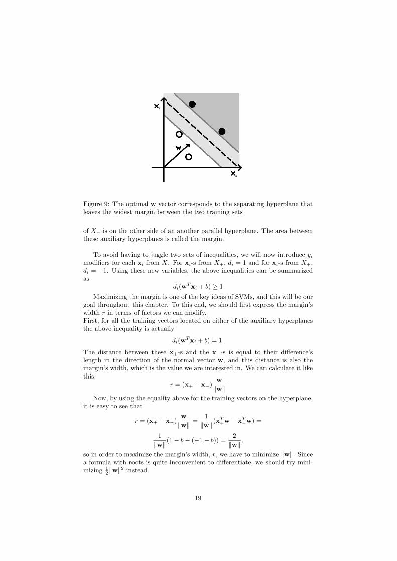
Figure 9: The optimal w vector corresponds to the separating hyperplane thatleaves the widest margin between the two training sets

of X− is on the other side of an another parallel hyperplane. The area betweenthese auxiliary hyperplanes is called the margin.

To avoid having to juggle two sets of inequalities, we will now introduce yimodifiers for each xi from X. For xi-s from X+, di = 1 and for xi-s from X+,di = −1. Using these new variables, the above inequalities can be summarizedas

di(wTxi + b) ≥ 1

Maximizing the margin is one of the key ideas of SVMs, and this will be ourgoal throughout this chapter. To this end, we should first express the margin’swidth r in terms of factors we can modify.First, for all the training vectors located on either of the auxiliary hyperplanesthe above inequality is actually

di(wTxi + b) = 1.

The distance between these x+-s and the x−-s is equal to their difference’slength in the direction of the normal vector w, and this distance is also themargin’s width, which is the value we are interested in. We can calculate it likethis:

r = (x+ − x−)w

‖w‖Now, by using the equality above for the training vectors on the hyperplane,

it is easy to see that

r = (x+ − x−)w

‖w‖=

1

‖w‖(xT+w− xT−w) =

1

‖w‖(1− b− (−1− b)) =

2

‖w‖,

so in order to maximize the margin’s width, r, we have to minimize ‖w‖. Sincea formula with roots is quite inconvenient to differentiate, we should try mini-mizing 1

2‖w‖2 instead.

19

Let us alter the inequalities one last time, to gain a form better suited formultivariate minimization:

di(wTxi + b)− 1 ≥ 0

Now we are ready to face the problem: we are looking for the minimum of afunction with n variables, on a set bounded by the inequalities. The best toolsto use here are the Lagrange multipliers.

Generally, if we have some differentiable function f(x1, x2, ..., xn) = f(x),and we want to find its extreme points, a minimum or a maximum, then wecalculate its partial derivatives, arrange them in a vector called the gradient,and look for an x∗ where the gradient is equal to zero. This point is a finecandidate for a local minimum or maximum, but there is a chance that it isneither, that it is a saddle point, and further evaluation is needed. However, ifthe function’s domain is the whole Rn, then all the minimums and maximumshave a gradient of zero.Sadly, this is not the case if we look for the function’s extreme point on a regionbounded by differentiable restriction functions g(x)i. This point may fall eitherinside the region, which is the less interesting case for us, since then the gradientshould still be zero there. What makes our life hard right now is the fact thatwhen the minimum or the maximum is on the border of the region, where (someof )the g(x)is are equal to zero, the gradient in that point could take any value.This is the part where we turn to Lagrange multipliers.

This handy method utilizes the fact that the possible extreme point x∗ onthe boundary of the region enclosed by the restriction functions g(x)i = 0 ischaracterized by a peculiar feature. On that point, the gradient of f(x) is alinear combination of the gradients of the g(x)is.To better understand why this is true, let us consider the case where n = 2and there is only one constraint, g(x). Let the border be a circle, for example.Now the search for the extreme point x∗ is equal to looking for a contour lineof f(x), a curve defined by f(x) = c, which touches the circle, but does notintersect it. In the point where the two curves meet the gradient of f(x) andthe gradient of g(x) are parallel to each other, or, in other terms, there existsa λ that ∇f(x∗) = λ∇g(x∗) (we do not care about the case where any of themare null vectors). In other words,

∇f(x∗)− λ∇g(x∗) = 0

This train of thought also holds in n dimensions and for k restrictions, withthe λis as coefficients for a linear combination. Thus, in the extreme point x∗,the following must hold:

L(x) = ∇f(x∗)−k∑i=1

λi∇g(x∗)i = 0

Let us use this knowledge to create the Lagrangian form of our problem.

20

The function to minimize, with the boundaries included, is as follows:

L(w, b) =1

2‖w‖2 −

l∑i=1

αi(di(wTxi + b)− 1),

where αi are non-negative values. This formula is called the primal optimizationproblem.

Since we want to minimize this function with respect to the w vector andthe b value, we will now differentiate it separately according to these variables.We will then look for the optimal w∗ and the optimal b∗ where this derivative is0. Fortunately this function is quadratic in w, so we will not get stuck in localminima.

Let us differentiate L(w, b) by the vector w. This is equal to partially differ-entiating the multivariate function by all but one of its variables. By assemblingthese partial derivatives, ∂L

∂wjfor j = 1, ..., n in a vector, we get the gradient

vector of L(w, b),

∂L

∂w(w, b) = w−

l∑i=1

αidixi.

To find the minimum in w, let us see where this gradient is equal to zero.

w−l∑i=1

αidixi = 0

w∗ =

l∑i=1

αidixi

This means that the ideal weight vector w∗ is a linear combination of the trainingvectors. If we knew the Lagrange multipliers’ exact values, our problem wouldbe solved.On the other hand, the derivative of L(w, b) by its variable b is much simpler:

∂L

∂b= −

l∑i=1

αidi.

To find the minimum in b, let us equate this expression to zero.

0 =

l∑i=1

αidi

This might be helpful down the road.Now let us substitute this sum form of w∗ into L(w, b), and also let us expandit to gain the dual form of L(w, b), which only depends on the α vector.

L(w, b) =1

2‖w‖2 −

l∑i=1

αi(di(wTxi + b)− 1) =

21

1

2wTw−

l∑i=1

αidiwTxi −

l∑i=1

αidib+

l∑i=1

αidi =

1

2(

l∑i=1

αidixi)T (

l∑j=1

αidixi)−l∑i=1

αidi

l∑j=1

αidixTi xi − b

l∑i=1

αidi +

l∑i=1

αi

Since the first two expressions are the same amount multiplied by 12 and −1,

and the third one is equal to zero according to the derivative by b, the dual formof the problem is

L(α) = −1

2

l∑i=1

l∑j=1

αidiαidixTi xi +

l∑i=1

αi

with the conditions of αi ≥ 0 for i = 1, ..., l and 0 =∑li=1 αidi. These con-

straints are called the Karsh-Kuhn-Tucker conditions, which guarantee us thatmaximizing the dual form is equal to minimizing the primal form.

At this point we are free to solve this quadratic programming problem aswe see fit, usually by using some numerical software. The solution’s α∗i coef-

ficients determine the ideal weight vector w∗ =∑li=1 α

∗i dixi. The ideal bias,

b∗ is calculable by, for example, substituting this w∗ into one of the inequali-ties that contain a training vector located on one of the auxiliary hyperplanes:di((w

∗)Txi + b) = 1. This results in a simple equation for b∗.

Having acquired the ideal w∗ and b∗ parameters, our now complete SVMwill make its decisions as follows:

y = sgn((w∗)Tx + b∗) = sgn(

l∑i=1

α∗i dixTi x + b∗),

where x is an unlabeled element of the input space.

This decision rule shows how similar the SVM is to the basis function net-works, with the basis functions xTi x. In the SVM’s case, however, we do notchoose the number of basis functions arbitrarily, with a trial and error method:the α∗i coefficients determine the number of them, since many of these α∗i s willbe zero. It is apparent from the QP problem’s conditions that the only α∗i s witha chance of being positive are those corresponding to xis on the auxiliary hy-perplanes, that is, the ones for which the inequality holds sharply. This meansthe number of required basis functions may be much lower than the numberof training vectors, and this speeds up the SVM’s decision making process im-mensely. This favorable trait of the SVM is called sparsity. The training vectorswith positive coefficients, the ones who play a real part in the decision makingare called the support vectors.

Another notable characteristic of the SVM is also apparent from the deci-sion function: it only demands the unknown input vector’s dot product with thesupport vectors for its calculations, not the actual input vector itself. While itmay not be obvious at first glance why this is so significant, this feature makes

22

the SVM the powerful tool it is in real-world applications.Note how we only solved the linear classification problem in this chapter, some-thing we already have done with a much less sophisticated construct. Thisdependence on the dot product guarantees that the non-linearly separable casewill not be that different a problem.

3.1.2 Soft margin: the linearly mostly separable case

The SVM’s heart is the wide margin it provides between the accepted and therejected vectors. This margin lets it minimize both parts of the general errorwe discussed in the previous chapter, as it learns the training set and keeps itscomplexity low simultaneously.But what if some of the training vectors of the two sets are too close to eachother, so even the widest margin is too narrow, or, worse, if the training vectorsare not linearly separable? In this chapter we will relax the constraints a bit,letting some of the training vectors slip inside the margin, or even fall on thewrong side of the separating hyperplane. These methods are called soft marginSVMs, and while there are various versions in use, we will only discuss the mostsimple solution, sometimes called the C-SVM.

Let us modify the constraints on the training vectors’ desired answers withthese ξi ≥ 0 slack variables:

di(wTxi + b) ≥ 1− ξi,

for i = 1, ..., l. As we want these slack variables to remain relatively small,because the machine should still classify as well as possible, we will includethese slack variables in the function to minimize:

L(w, b, ξ) =1

2‖w‖2 + C

l∑i=1

ξi,

where C ≥ 0 is some constant that determines how much we penalize the mis-classifications and the vectors wandering into the margin. It is chosen arbitrarily,and it represents how much are we willing to sacrifice in order to keep a widemargin. Note how for C = 0, meaning we do not compromise, the problem isthe original linear classification.Now let us use Lagrange multipliers once again:

L(w, b) =1

2‖w‖2 + C

l∑i=1

ξi −l∑i=1

αi(di(wTxi + b)− 1 + ξi)−

l∑i=1

γiξi

This time, in addition to the first two, we have to differentiate this function byits third group of variables, the ξis.

∂L

∂ξi= C − αi + γi

for i = 1, ..., l. This yields the following optimality criteria:

0 = C − αi + γi

23

C = αi + γi

This means that by calculating the αis, we also get the corresponding γisthrough the simple formula γi = C − αi.In this case the dual form only differs in one of the constraints: instead of simplylooking for any αi ≥ 0, we put a cap on these αis, so the new constraint is

0 ≤ αi ≤ C

for i = 1, ..., l. The non-negativity of the γis demands this constraint, but thisis the only way the relaxation affects the dual form.

Now we should solve this quadratic problem as we see fit. In this case, how-ever, the support vectors are not necessarily those on the auxiliary hyperplanes.This time they are those for which

di(wTxi + b) = 1− ξi

holds.

Choosing an appropriate C for relaxation is a problem in itself. It requiressome kind of heuristic method, trying many C-s until we find one that leaves asufficiently wide margin without letting too many training vectors go astray.Despite these further complications in training, soft margin SVMs are just aspopular as they are useful. In most implementations, built-in SVMs have twodefining parameters to choose arbitrarily by the user, and one of these is therelaxation parameter. We will discuss the other one, the feature that lies in theheart of the SVM in the next part.

3.2 Nonlinear SVM

3.2.1 Feature map: transforming the problem

Let us assume that the training vectors are very non-linearly separable, that theyare so intertwined that simply softening the margin would distort the problembeyond recognition, for example if all of X+ is located inside a sphere, and allof X− is scattered outside of it, in all directions. This is a very realistic scenarioin classification problems, so our model should be ready to tackle it.

First, we should recall an idea we have discussed in the previous part: basisfunctions. Their primary role was to transform the input vectors into a spacewhere they are linearly separable, even at the cost of increasing their dimension.So, this time, instead of working with n-dimensional xis, we apply some basisfunction Φ = (φ1, φ2, ..., φm) : Rn → Rm on all of them, and use the resultingm-dimensional Φ(xi)s.This possibly dimension-expanding function is called the feature map, and itsrange is the feature space. This name suggests how the function should somehowemphasize the input vectors’ important features, for example, if our machineshould somehow prefer shorter vectors, and reject longer ones, then the featurespace could be R+, and the feature map is Φ(x) = (‖x‖. In this special case,

24

the dimension actually shrinks, contrary to the usual.

Let us see how this transformation changes the constraints from the lastchapter:

di(wTΦ(xi) + b) ≥ 1.

Using these transformed vectors, the problem is equal to a linearly separableone in the feature space, which is also know as the feature space. This meansthe optimal - now m − 1 dimensional - separating hyperplane’s normal vectorw∗ is a linear combination of the transformed training vectors:

w∗ =

l∑i=1

α∗i diΦ(xi).

We can find the optimal α∗i coefficients the same way as before, throughsolving the quadratic optimization problem, and this will yield the followingdecision function for the unlabeled vector x:

y = sgn(

l∑i=1

α∗i diΦ(xi)TΦ(x) + b∗).

Of course, most of the α∗i s will be zeros this time too, and the support vectors’Φ(xi) forms will lie on the auxiliary hyperplanes in the feature space, and inthe input space they will fall on the border of the non-linear margin.

Note how the decision function above only uses the Φ transformation im-plicitly, through the inner products: we only need the inner product of thetransformed Φ(xi) and Φ(x) vectors, not the transformed vectors themselves.This observation makes solving the non-linear case immensely easier, becauseit means that if we had a function K(xi,x) = Φ(xi)

TΦ(x) that calculates thetransformed vectors’ inner products directly, then we could save both computa-tional power and a significant amount of headache caused by trying to appraisethe characteristics of the feature space.

3.2.2 Kernel trick

These K(xi,x) functions are called kernel functions. While the feature spacemay be very complex, and even of infinite dimension, the corresponding kernelfunction could be simple and easily calculable. This benevolent effect of usingkernel functions instead of the basis functions is referred to as the ”kernel trick”.The decision function using the kernel trick is:

y = sgn(

l∑i=1

α∗i diK(xi,x) + b∗).

Now let us see what functions are fit to be used as kernels. Of course, theyshould stand for a dot product in some space, but how do we determine abouta given function if there exists such a space?To get more familiar with kernel functions, let us arrange the K(xi,xj) valuesfor all elements of the training set X in the kernel matrix K. According to the

25

Figure 10: The two-degree polynomial kernel in use [6]

assumption that this kernel function stands for a dot product in some unknownspace, endowed with all of its dot product traits, K is symmetric. If it satisfiesMercer’s condition, that is, it is also positive semi-definite, then K(x,y) is adot product for some space, and thus a valid kernel function.

Mercer’s theorem also provides us with a theoretical method of identifyingthe underlying feature map Φ(x), for which K(x,y) = Φ(x)TΦ(y), for a givenpositive semi-definite kernel function.Let the input space X be a closed subset of Rn. If a symmetric, continuousK(x,y) function is positive semi-definite, meaning for all x1,x2, ...,xk elementsof the input space and any c1, c2, ..., ck real numbers

k∑i=1

k∑j=1

K(xi,xj)cicj ≥ 0,

and also ∫X

∫X

K(x,y)2dxdy,

then we can define an integral operator

LK(f(x)) =

∫X

K(x, t)f(t)dt

for all f(x) from L2(X). This is a self-adjointed, non-negative compact oper-ator on L2(X), so, according to the spectral theory of compact operators, itseigenvalues λi are non-negative and square-summable, and its eigenfunctionsφ(x)iare orthonormal and they form a base in L2(X).Mercer’s theorem states that the kernel function can be represented with theseeigenfunctions as

K(x,y) =

∞∑i=1

λiφ(x)iφ(y)i,

and the converge is absolute and uniform on each compact subset of X.

In practice, a kernel function should measure some kind of similarity betweenits variables. This means it should be

26

• symmetric: K(xi,xj) = K(xi,xj)

• non-negative: K(xi,xj) ≥ 0

• maximal if the variables are the same: K(xi,xi) ≥ K(xi,xj)

One of the simplest kernels are the polynomial kernels. In their most basicform, called homogeneous polynomial kernels, they are

K(x,y) = (xTy)d,

where d ≥ 1 is a natural number. For d = 1 this kernel is the dot product of itsinputs, so using it results in the linear SVM. Let us expand this expression ford = 2:

K(x,y) = (xTy)2 = (

n∑i=1

xiyi)2 =

n∑i=1

x2i y2i +

n∑i=2

i−1∑j=1

2xiyixjyj

They are called homogeneous because all of its terms are the same degree. Toinclude all terms up to d in the kernel, one must use an inhomogeneous kernel:

K(x,y) = (xTy + c)2 = (

n∑i=1

xiyi + c)2,

where c is a positive real parameter, and it defines how much influence we wouldlike the lower degree terms to have compared to the higher degree terms.

Let us backtrack the Φ(x) feature map this one time, for the homogeneousd = 2 case:

Φ(x) = (x21, x22, ..., x

2n,√

2x1x2,√

2x1x2, ...,√

2xn−1xn).

It is easy to see how rapidly the feature space’s dimension grows: if the inputspace’s dimension is n, then it increases to nd. This case illustrates how evenwhen computing the actual Φ(x)s is not feasible, the kernel function K(x,y)can be well within our reach. With homogeneous polynomial kernels, it meansthat instead of nd computations to map the vector into the feature space, andexecuting the dot product there, we need only to calculate the original dot prod-uct an then raise it the power d.

Another popular kernel is the RBF kernel, also called the Gaussian kernel.It depends on the Euclidean distance between its variables, and while its featurespace is of infinite dimensions, in practice it’s useful and readily calculable. Itis usually written as

K(x,y) = exp(−‖x− y‖2

2σ2),

for some real parameter σ. Note how similar the SVM becomes to the RBFnetwork if we use this kernel, hence the name. We can also imitate the MLPwith another special kernel, the sigmoid kernel:

K(x,y) = tanh(kx)TΦ(y + θ).

27

This kernel is not positive semi-definite for every combination of its parameters,so they must be chosen carefully.

The truly marvelous thing about kernel functions is the fact that they canbe generalized into any similarity measure, as long as it makes sense and iseasily computable on the elements of the input space. For example, the so-called string kernels are extremely useful in text processing. Their feature mapsextract words, phonemes, or shorter word combinations with respect to theirorder in the original strings, and the kernels themselves measure how hard it isto transform one of the strings to the other. This method can compare stringsof different lengths.Similarly, there are graph kernels that measure the difference between twographs, and tree kernels specialized on rooted trees.

4 Implementations & Applications

4.1 Implementations

4.1.1 ANN Software

There are numerous approaches to implementing neural methods.One of these are the simulator softwares, whose primary purpose is to illustratewhat the machine looks like, and to gain a better understanding of how it works.They have graphical user interfaces and they are more intuitive to learn and use.One of such simulators is the Stuttgart Neural Network Simulator (SNNS), de-veloped at the University of Stuttgart.Usually they are self-contained, and programs produced using them cannot beintegrated very well into grater projects. This unfortunate trait made them losetheir popularity over time.

Still, such an isolated approach could be used to simulate a biological net-work. Programs dedicated to this effort include Neuron and GENESIS.

If our goal, however, is only to exploit the data mining abilities of neuralnetworks, we should turn to more generic machine learning software.Very extensive ANN implementations can be found in the Neural Network Tool-box of Matlab, but if one is looking for open-source programs, the OpenCVlibrary is free, multi-platform collection of learning algorithms. Developed byIntel, it is mainly focused on computer vision, hence the name.A similar open-source project is OpenNN, currently developed by Intelnics, witha focus on neural networks. It has won two awards in 2014 for being an efficientdata mining tool.

4.1.2 Hardware implementations

In the ’60s two engineers, Bernard Widrow and his doctoral student Ted Hoffbuilt the adaline, the first neural network to exist as more than a theoretical

28

tool. Liquid-based memristors represented the adjustable weights, and the ma-chine was able to discriminate crude geometric shapes, translate speech intotext, forecast weather, balance a broom standing on its head, and even to playblackjack.[7]

Recently, modern memristor-based implementations are under development.IBM Research, Hewlett-Packard and HRL Laboratories are working on projectSyNAPSE, funded by the DARPA, a US military research agency. The project’sgoal is to create neuromorphic computer chips with the characteristics of a mam-malian brain: low energy consumption paired with high performance.While generally neuromorphic programming’s aim is to imitate the human brain,SyNAPSE takes a step towards abstraction: the researchers concern themselvesless with simulation, as they would rather take hold of the advantages a biologicprocessing system enjoys.

The chip they have constructed, TrueNorth, contains a million neurons,each with 256 synapses, grouped into 4096 cores.[8] All of these nanometer scalesynapses have adjustable weights, which makes the chip capable of learning.The cores are arranged into a two-dimensional array, and they communicate inan event-driven manner, unlike the traditional clock-based von Neumann sys-tems.

SyNAPSE’s long-term goal is building a neuro-synaptic system of billions ofneurons that still consumes one kilowatt of power.They also plan on fusing traditional computer technology, based on analyticalthinking, with neuromorphic chips, representing pattern recognition, thus cre-ating a new intelligence whose abilities surpass both.

4.2 Applications

4.2.1 Traditional and modern uses

The ANNs have made their way into many computational tasks, with varyingsuccess.

Their classical applications, the tasks they were created for are problemspertaining to artificial intelligence. They include pattern classification, cluster-ing, function approximation, forecasting, optimization, associative memory andcontrol.[9]

Nowadays, biology and medicine have discovered ANNs and the SVM.In modern biology, information technology and mathematics have a greater rolethan ever, as new research methods produce vast amounts of data to analyze.This data is often disorganized, and interpreting the results demands elaboratenew methods.

One of the greatest challenges of biologists is protein classification. Proteinshave received great attention in the recent decades, as they are responsible foralmost all things our cells do. They serve as carriers and catalysts in living crea-

29

Figure 11: The different levels of protein structure. Ideally, at some point wemay be able to predict the three higher forms from the primary sequence, andmaybe even backtrack the sequence from the higher forms. [10]

tures’ biological processes, and understanding them could help cure diseases anddevelop more efficient ways to tame nature.

Their versatility and diversity, however, makes them hard to study. In sim-ple terms, each protein consists of a few hundreds or thousands of amino acids,arranged in a given order. This sequence of amino acids is called the primarystructure. Researchers are more interested in the higher level structures, as theycorrespond to the shape the protein takes when it is synthesized and ready towork. Another point of interest is the correspondence between a protein’s aminoacid sequence and its 3-dimensional structure. This is more of a mathematicalproblem than a biological one, and a very difficult one at that.

Protein classification is the problem of determining a given protein’s func-tion and location in the cell from some research data, such as its amino acidsequence, amino acid composition (how many of the 20 kinds of amino acidsdoes it consist of, or in what ratio does it contain them), or some vague infor-mation about its shape.This is a field where ANNs, and the SVM could be deployed, as we have massiveamounts of noisy data and yes-or-no questions, such as: could this protein belocated in the nucleus? Could it work as an enzyme in this reaction?

SVMs are at work in determining protein structure from their amino acidcomposition. [11]An online functional classifier that makes its assumptions based on amino acidsequence can be found at [12].

Neural networks have found their uses in modern medicine, too. As an ad-vanced data mining method, they help the doctors in diagnosis and prognosisin case of illnesses with no effective diagnostic tools.[13]ANNs have been used to diagnose cancer, and the SVM to diagnose psychiatricdiseases.

30

4.2.2 Interpreting the model

As a counterpoint to their versatility, the difficulty of their interpretation is aserious drawback of using neural networks. Simply put, they do their work,they draw their mostly correct conclusions from the input, but they do not tellhow they do it.We may be lucky enough to use a software that visualizes the complex systemof weights the machine is made of, and we could look for important nodes andedges, but in a multi-layered network that is little consolation.

SVMs are a bit more helpful in this respect: by selecting the support vectors,they highlight some data points for us. In the psychiatric study I have mentionedpreviously the researchers have tried training the SVM with multiple subsets ofthe data at hand, to decide which features yield the most precise classifier. Theytheorized that these features and their relation to diseases should be examinedmore thoroughly.This example shows how there is a natural need for an interpretation of themachine’s results: it is helpful to have a network to make guesses for us, butwe would like to know on what basis does it make its decisions. What are itsregions of interest, what patterns does it notice that eludes human observers?

Without a sufficient answer to these questions, the network remains a blackbox, a magic oracle to consult. Such an adviser is hard to trust, even if it isright most of the time.

Let us finish with a cautionary tale about a failed experiment with artificialneural networks.In the 1980s, the Pentagon has tried to build a network that could recognizeenemy tanks hiding behind trees. The computer scientists who were tasked withcreating this machine went out, and took photos of trees with or without tankslurking behind them.They first trained the network with half of these photos, until it has learned toclassify them sufficiently. Afterwards, for testing, they used the remaining pic-tures. They were relieved to see that the machine has not only learned the testexamples, but was able to generalize its knowledge to the previously unknowndata. They submitted their creation to the Pentagon.The Pentagon, suspicious as always, took new pictures, and tested the machinewith them. The results were embarrassingly random. It took a while for theashamed computer scientists to find out what was the problem.They looked at all the photos they used to teach and to test their system: thepictures with tanks in them were taken on a cloudy day, and on all the othersthe sky was clear, and the sun was shining. They have accidentally taught thenetwork to tell what the weather was like.[14]

4.3 A conclusion

Machine learning’s aim is to recreate the living organism’s superior ability oflearning, of generalizing its knowledge and adapting to its environment.Doing so is equal to letting go of the certainty of a classic, high level, instruction-

31

based computational model in favor of a probabilistic one. It means that wecannot predict what the intelligence we create will end up like, of how it willsee best to operate, and how well it will be able to negotiate the obstacles weput in its way.While there is a great danger in this approach, it also opens up myriads ofpossibilities: a deep-learning architecture could see patterns where we cannot,could solve problems that we can hardly formalize.

The recent successes of such machines show that the field merits out atten-tion. Computer science companies such as Google and Microsoft initiate deeplearning research in vision, speech recognition and drug discovery.Even though artificial intelligence has a reputation of going through cycles ofhype and disillusionment, machine learning may very well play a huge part inthe future of computing.

References

[1] Hubert Eichner, 2014.

[2] B. Yegnanarayana. Artificial Neural Networks. Prentice Hall of India, NewDelhi, 2006.

[3] David Leverington. A basic introduction to feedforward backpropagationneural networks, 2009.

[4] Robert Hecht-Nielsen. Neurocomputing. Addison-Wesley, 1990.

[5] Jonathan Richard Shewchuk. An introduction to the conjugate gradientmethod without the agonizing pain, 1994.

[6]

[7] Bernard Widrow. Birth, life and death in microelectronic systems, 1961.

[8] Dharmendra S. Modha et al. Cognitive computing building block: A ver-satile and efficient digital neuron model for neurosynaptic cores. 2013.

[9] Anil K. Jain and Jianchang Mao. Artificial neural networks: A tutorial.1996.

[10]

[11] Xue-biao Xu Yu-Dong Cai, Xiao-Jun Liu and Guo-Ping Zhou. Supportvector machines for predicting protein structural class. 2001.

[12] Bioinformatics and Drug Design Group. Svmprot: Protein functional fam-ily prediction, 2003.

[13] W. G. Baxt MD. Application of artificial neural networks to clinicalmedicine. 1995.

[14] Neil Fraser. Neural network follies, 1998.

32

[15] Christopher J.C. Burges. A tutorial on support vector machines for patternrecognition. 1998.

[16] Horvath Gabor, Pataki Bela, Strausz Gyorgy, Takacs Gabor, Valyon Jozsef,and Altrichter Marta. Neuralis halozatok. Panem Konyvkiado Kft., Bu-dapest, 2006.

[17] James E. Gentle, Wolfgang Karl Hardle, and Yuichi Mori. Handbook ofComputational Statistics. Springer, Berlin, 2007.

[18] Ha Quang Minh, Partha Niyogi, and Yuan Yao. Mercer’s theorem, featuremaps, and smoothing. 2006.

[19] Dan Klein. Lagrange multipliers without permanent scarring. Permanentlyin rough draft form.

33