MNRAS 485, 5153–5167 (2019) doi:10.1093/mnras/stz645Advance Access publication 2019 March 7

Keck HIRES spectroscopy of SkyMapper commissioning surveycandidate extremely metal-poor stars

A. F. Marino ,1,2,3‹ G. S. Da Costa ,1 A. R. Casey ,1,4,5 M. Asplund ,1,6

M. S. Bessell ,1 A. Frebel ,7 S. C. Keller,1 K. Lind,8,9 A. D. Mackey,1

S. J. Murphy ,1,10 T. Nordlander,1,6 J. E. Norris,1 B. P. Schmidt 1 and D. Yong 1

1Research School of Astronomy & Astrophysics, Australian National University, ACT 2611, Australia2Dipartimento di Fisica e Astronomia ‘Galileo Galilei’ – Univ. di Padova, Vicolo dell’Osservatorio 3, Padova, IT-35122, Italy3Centro di Ateneo di Studi e Attivita Spaziali ‘Giuseppe Colombo’ – CISAS, Via Venezia 15, Padova, IT-35131, Italy4School of Physics and Astronomy, Monash University, Wellington Rd, Clayton, VIC 3800, Australia5Faculty of Information Technology, Monash University, Wellington Rd, Clayton, VIC 3800, Australia6Center of Excellence for Astrophysics in Three Dimensions (ASTRO-3D), Australia7Department of Physics and Kavli Institute for Astrophysics and Space Research, Massachusetts Institute of Technology, Cambridge, MA 02139, USA8Max-Planck-Institut fur Astronomie, Konigstuhl 17, D-69117 Heidelberg, Germany9Observational Astrophysics, Department of Physics and Astronomy, Uppsala University, Box 516, SE-751 20 Uppsala, Sweden10School of Physical, Environmental and Mathematical Sciences, University of New South Wales, Canberra, ACT 2600, Australia

Accepted 2019 February 25. Received 2019 February 4; in original form 2018 December 2

ABSTRACTWe present results from the analysis of high-resolution spectra obtained with the Keck HIRESspectrograph for a sample of 17 candidate extremely metal-poor (EMP) stars originally selectedfrom commissioning data obtained with the SkyMapper telescope. Fourteen of the starshave not been observed previously at high dispersion. Three have [Fe/H] ≤ −3.0, whilethe remainder, with two more metal-rich exceptions, have −3.0 ≤ [Fe/H] ≤ −2.0 dex. Apartfrom Fe, we also derive abundances for the elements C, N, Na, Mg, Al, Si, Ca, Sc, Ti, Cr, Mn,Co, Ni, and Zn, and for n-capture elements Sr, Ba, and Eu. None of the current sample of starsis found to be carbon-rich. In general, our chemical abundances follow previous trends foundin the literature, although we note that two of the most metal-poor stars show very low [Ba/Fe](∼−1.7) coupled with low [Sr/Ba] (∼−0.3). Such stars are relatively rare in the Galactic halo.One further star, and possibly two others, meet the criteria for classification as a r-I star. Thisstudy, together with that of Jacobson et al. (2015), completes the outcomes of the SkyMappercommissioning data survey for EMP stars.

Key words: stars: abundances – stars: Population II – Galaxy: halo – Galaxy: stellar content.

1 IN T RO D U C T I O N

As reviewed by Frebel & Norris (2015), the detailed study ofthe most metal-poor stars in the Galaxy can provide vital cluesto the processes of star formation and to the synthesis of thechemical elements at the earliest times. Such stars, however, areextremely rare and at the present time only a handful are known with[Fe/H] ≤−4.5 dex. The importance of these objects has neverthelessprompted a number of previous and ongoing searches for suchextremely metal-poor (EMP) stars [e.g. the HK survey (Beers,Preston & Shectman 1992), the HES (Frebel et al. 2006; Christliebet al. 2008), the SDSS (see Aoki et al. 2013), the ‘Best and Brightest’survey (Schlaufman & Casey 2014), LAMOST (see Li et al. 2015a),

� E-mail: anna.marino@unipd.it

and Pristine (Starkenburg et al. 2017), and references therein]. Thediscovery of such stars is one of the prime science drivers behindthe SkyMapper imaging survey of the Southern hemisphere sky(Keller et al. 2007; Wolf et al. 2018). The metallicity sensitivityis achieved through the incorporation of a relatively narrow v-filter, whose bandpass includes the Ca II H and K lines, into theSkyMapper filter set (Bessell et al. 2011). The SkyMapper uvgrizphotometric survey of the southern sky is ongoing (Wolf et al.2018) but during the commissioning of the telescope a number ofvgi images were taken to search for EMP candidates. Despite thesub-optimal quality of many of the images, the program, whichwe will refer to as the ‘SkyMapper commissioning survey forEMP-stars’ (to distinguish it from the current ongoing work), wassuccessful in that it resulted in the discovery of the currently most-iron poor star known SMSS J031300.36–670839.3 (Keller et al.2014; Bessell et al. 2015; Nordlander et al. 2017). The analysis

C© 2019 The Author(s)Published by Oxford University Press on behalf of the Royal Astronomical Society

Dow

nloaded from https://academ

ic.oup.com/m

nras/article-abstract/485/4/5153/5371160 by MIT Libraries user on 22 July 2019

5154 A. F. Marino et al.

Table 1. Details of the target stars and the Keck HIRES observations.

ID RA Dec. g (g − i)0 mi Exp Time S/N [450 nm] S/N [600 nm] RV(J2000)(h:m:s) (J2000)(o:′:′′) (s) (pix−1) (pix−1) (km s−1) Notes

SMSS J202059.17–043447.0 20:20:59.17 − 04:34:47.0 13.815 0.837 0.243 660 34 38 − 190.7SMSS J202400.03–024445.9 20:24:00.03 − 02:44:45.9 15.631 0.850 0.235 660 15 17 − 133.8SMSS J202601.44–033002.5 20:26:01.44 − 03:30:02.5 15.508 0.541 0.140 1800 21 26 − 149.5SMSS J202659.41–031149.2 20:26:59.41 − 03:11:49.2 14.180 0.641 0.027 600 28 29 − 199.1SMSS J204654.92–020409.2 20:46:54.92 − 02:04:09.2 15.026 0.882 0.131 1200 26 30 − 451.2SMSS J211657.83–012517.5 21:16:57.83 − 01:25:17.5 14.515 0.675 − 0.054 900 21 22 − 155.4SMSS J212001.71–001158.6 21:20:01.71 − 00:11:58.6 15.582 0.942 0.134 1500 22 26 − 350.2SMSS J212113.63–005132.2 21:21:13.63 − 00:51:32.2 14.854 0.712 0.002 1200 21 23 +33.9SMSS J212217.52–295552.7 21:22:17.52 − 29:55:52.7 16.387 0.554 0.040 2700 18 19 +200.8SMSS J220514.10–013407.6 22:05:14.10 − 01:34:07.6 13.933 0.802 0.225 600 22 26 − 199.2SMSS J220535.05–004403.6 22:05:35.05 − 00:44:03.6 14.214 0.704 0.043 600 25 28 − 62.2SMSS J221334.13–072604.1 22:13:34.13 − 07:26:04.1 15.310 0.759 0.072 1500 19 22 − 392.7 1SMSS J222349.48–114751.1 22:23:49.48 − 11:47:51.1 15.177 0.719 0.028 1500 22 23 − 367.1SMSS J225336.83–270435.4 22:53:36.83 − 27:04:35.4 16.024 0.685 0.022 1500 16 17 +116.6SMSS J230306.22–041621.8 23:03:06.22 − 04:16:21.8 14.606 0.699 0.003 1200 26 28 − 244.6SMSS J010839.58–285701.5 01:08:39.58 − 28:57:01.5 12.747 0.615 0.033 300 34 35 +144.3 2SMSS J034249.52–284215.8 03:42:49.52 − 28:42:15.8 14.646 0.676 0.108 1200 29 31 +157.2 2

Notes: (1) In Aoki et al. (2013) as SDSS J2213–0726; and (2) in Jacobson et al. (2015)

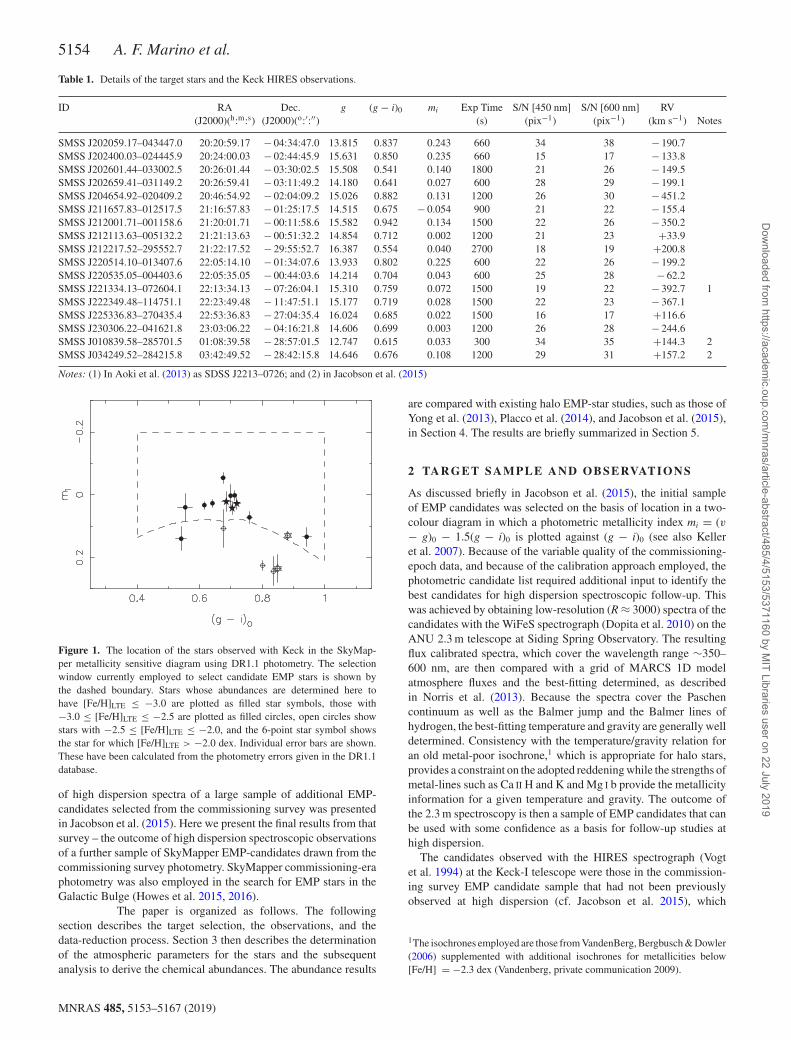
Figure 1. The location of the stars observed with Keck in the SkyMap-per metallicity sensitive diagram using DR1.1 photometry. The selectionwindow currently employed to select candidate EMP stars is shown bythe dashed boundary. Stars whose abundances are determined here tohave [Fe/H]LTE ≤ −3.0 are plotted as filled star symbols, those with−3.0 ≤ [Fe/H]LTE ≤ −2.5 are plotted as filled circles, open circles showstars with −2.5 ≤ [Fe/H]LTE ≤ −2.0, and the 6-point star symbol showsthe star for which [Fe/H]LTE > −2.0 dex. Individual error bars are shown.These have been calculated from the photometry errors given in the DR1.1database.

of high dispersion spectra of a large sample of additional EMP-candidates selected from the commissioning survey was presentedin Jacobson et al. (2015). Here we present the final results from thatsurvey – the outcome of high dispersion spectroscopic observationsof a further sample of SkyMapper EMP-candidates drawn from thecommissioning survey photometry. SkyMapper commissioning-eraphotometry was also employed in the search for EMP stars in theGalactic Bulge (Howes et al. 2015, 2016).

The paper is organized as follows. The followingsection describes the target selection, the observations, and thedata-reduction process. Section 3 then describes the determinationof the atmospheric parameters for the stars and the subsequentanalysis to derive the chemical abundances. The abundance results

are compared with existing halo EMP-star studies, such as those ofYong et al. (2013), Placco et al. (2014), and Jacobson et al. (2015),in Section 4. The results are briefly summarized in Section 5.

2 TARGET SAMPLE AND OBSERVATI ONS

As discussed briefly in Jacobson et al. (2015), the initial sampleof EMP candidates was selected on the basis of location in a two-colour diagram in which a photometric metallicity index mi = (v− g)0 − 1.5(g − i)0 is plotted against (g − i)0 (see also Kelleret al. 2007). Because of the variable quality of the commissioning-epoch data, and because of the calibration approach employed, thephotometric candidate list required additional input to identify thebest candidates for high dispersion spectroscopic follow-up. Thiswas achieved by obtaining low-resolution (R ≈ 3000) spectra of thecandidates with the WiFeS spectrograph (Dopita et al. 2010) on theANU 2.3 m telescope at Siding Spring Observatory. The resultingflux calibrated spectra, which cover the wavelength range ∼350–600 nm, are then compared with a grid of MARCS 1D modelatmosphere fluxes and the best-fitting determined, as describedin Norris et al. (2013). Because the spectra cover the Paschencontinuum as well as the Balmer jump and the Balmer lines ofhydrogen, the best-fitting temperature and gravity are generally welldetermined. Consistency with the temperature/gravity relation foran old metal-poor isochrone,1 which is appropriate for halo stars,provides a constraint on the adopted reddening while the strengths ofmetal-lines such as Ca II H and K and Mg I b provide the metallicityinformation for a given temperature and gravity. The outcome ofthe 2.3 m spectroscopy is then a sample of EMP candidates that canbe used with some confidence as a basis for follow-up studies athigh dispersion.

The candidates observed with the HIRES spectrograph (Vogtet al. 1994) at the Keck-I telescope were those in the commission-ing survey EMP candidate sample that had not been previouslyobserved at high dispersion (cf. Jacobson et al. 2015), which

1The isochrones employed are those from VandenBerg, Bergbusch & Dowler(2006) supplemented with additional isochrones for metallicities below[Fe/H] = −2.3 dex (Vandenberg, private communication 2009).

MNRAS 485, 5153–5167 (2019)

Dow

nloaded from https://academ

ic.oup.com/m

nras/article-abstract/485/4/5153/5371160 by MIT Libraries user on 22 July 2019

Keck spectroscopy of SkyMapper EMP candidates 5155

Figure 2. Top panel: the adopted corrected spectroscopic temperatures areshown as a function of the temperatures obtained from spectral fits to thelow-resolution 2.3 m spectra. The dashed line is the 1:1 relation. Middlepanel: the adopted spectroscopic gravities are plotted against the log g valuesderived from the fits to the low-resolution spectra. The dashed line is the 1:1relation. Bottom panel: a comparison of the [Fe/H]LTE values determinedfrom the Keck spectra with those estimated from the low-resolution spectralfits. The dashed line is again a 1:1 relation.

were accessible from the Keck Observatory on the scheduled dateand which had low-resolution spectroscopic abundance estimates[Fe/H]2.3m ≤ −2.5 dex, as determined from the 2.3m spectra. Inall, HIRES spectra were obtained for 15 candidate EMP stars onthe ANU-allocated night of 2013 September 21 (UT), together withspectra of two stars that had also been observed at Magellan withthe MIKE spectrograph in the Jacobson et al. (2015) study. Onefurther star, SMSS J221334.13–072604.1, was subsequently foundto be included in the sample analysed by Aoki et al. (2013) underthe designation SDSS J2213–0726.

Observing conditions were good with the seeing slowly risingfrom 0.6 to 1 arcsec by the end of the night. The spectrograph wasconfigured with the HIRESb cross-disperser and the C1 decker thathas a slit width of 0.86 arcsec yielding a resolution R ≈ 50 000.Detector binning was 2 (spatial) × 1 (spectral) and the low-gainsetting (∼2e−/DN) was used for the three CCDs in the detectormosaic. Details of the observations are given in Table 1. The tablelists the SkyMapper survey designations, the positions, and theSkyMapper g, (g − i)0 and mi photometry taken from the SkyMap-per DR1.1 data release (Wolf et al. 2018), which supersede theoriginal commissioning-era photometry. The reddening correctionsfollow the procedure outlined in Wolf et al. (2018) while mi is themetallicity index, defined as (v − g)0 − 1.5(g − i)0, for whichmore negative values at fixed colour indicate potentially lowermetallicity (see Keller et al. 2007; Da Costa et al. ). Also given arethe integration times and the S/N per pixel of the reduced spectraat 450 and 600 nm. The median values are 22 pix−1 at 450 nm and26 pix−1 at 600 nm.

In Fig. 1 we show the location of the observed stars in theSkyMapper metallicity-sensitive diagram based on the DR1.1photometry. Shown also in the figure is the selection window thatis used in defining photometric EMP candidates for the current(post-commissioning) survey, where the lower boundary is setby the location of the [M/H] = −2.0 dex, 12.5 Gyr isochronein this plane (see Da Costa et al., in preparation for details).While photometric uncertainties, particularly in the v-magnitudes,introduce scatter in this diagram, it is reassuring that all but 1of the 12 candidates that are found in the analysis here to have[Fe/H]LTE ≤ −2.5 dex (where LTE means that the Fe abundance isobtained assuming the local thermodynamic equilibrium, LTE) arewithin the selection window while there is only one contaminant– a star found here to have [Fe/H]LTE > −2.0 despite lying (just)in the selection region. Although the sample is small, Fig. 1 doesverify that the current SkyMapper photometric selection processefficiently finds stars with [Fe/H]LTE ≤ −2.5 with only a very minordegree of contamination. In fact, Da Costa et al. () show that in thecurrent ongoing program, ∼85 per cent of the SkyMapper DR1.1photometric EMP candidates that lie within the selection windowshown in Fig. 1, and which also possess metallicity estimates fromlow-resolution 2.3 m spectra, have [Fe/H]2.3m ≤ −2.0 dex, while∼40 per cent have [Fe/H]2.3m ≤ −2.75 dex. The best candidatesare then followed up at high dispersion with the MIKE echellespectrograph on the Magellan 6.5 m telescope.

The observed spectra were processed with the standard HIRESreduction pipeline MAKEE to obtain flat-fielded, extracted,wavelength-calibrated, velocity-corrected spectra for each echelleorder. For the subsequent analysis, the individual spectral orderswere merged into a single continuous spectrum for each of thethree CCD detectors, which was then continuum normalized andwavelength-offset by the observed geocentric velocity.

Radial velocities (RVs) were derived using the IRAF@FXCORtask, which cross-correlates the object spectrum with a template

MNRAS 485, 5153–5167 (2019)

Dow

nloaded from https://academ

ic.oup.com/m

nras/article-abstract/485/4/5153/5371160 by MIT Libraries user on 22 July 2019

5156 A. F. Marino et al.

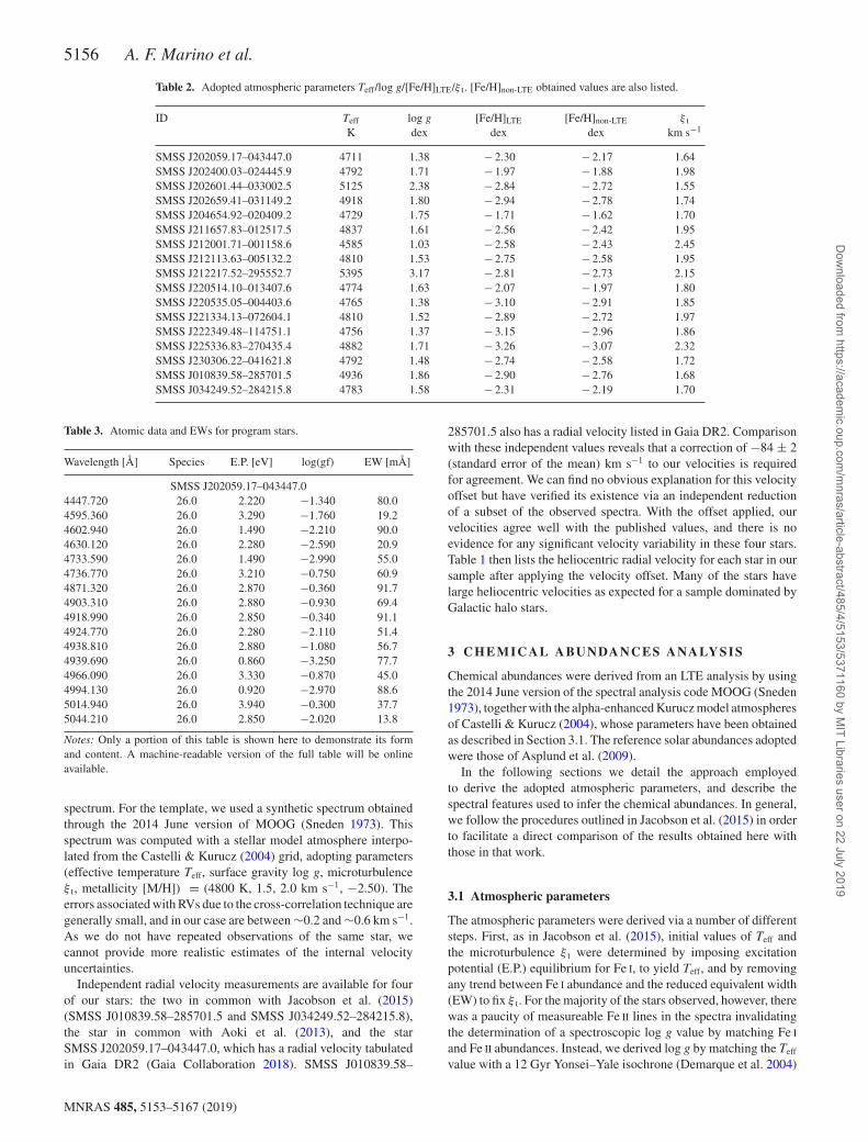
Table 2. Adopted atmospheric parameters Teff/log g/[Fe/H]LTE/ξ t. [Fe/H]non-LTE obtained values are also listed.

ID Teff log g [Fe/H]LTE [Fe/H]non-LTE ξ t

K dex dex dex km s−1

SMSS J202059.17–043447.0 4711 1.38 − 2.30 − 2.17 1.64SMSS J202400.03–024445.9 4792 1.71 − 1.97 − 1.88 1.98SMSS J202601.44–033002.5 5125 2.38 − 2.84 − 2.72 1.55SMSS J202659.41–031149.2 4918 1.80 − 2.94 − 2.78 1.74SMSS J204654.92–020409.2 4729 1.75 − 1.71 − 1.62 1.70SMSS J211657.83–012517.5 4837 1.61 − 2.56 − 2.42 1.95SMSS J212001.71–001158.6 4585 1.03 − 2.58 − 2.43 2.45SMSS J212113.63–005132.2 4810 1.53 − 2.75 − 2.58 1.95SMSS J212217.52–295552.7 5395 3.17 − 2.81 − 2.73 2.15SMSS J220514.10–013407.6 4774 1.63 − 2.07 − 1.97 1.80SMSS J220535.05–004403.6 4765 1.38 − 3.10 − 2.91 1.85SMSS J221334.13–072604.1 4810 1.52 − 2.89 − 2.72 1.97SMSS J222349.48–114751.1 4756 1.37 − 3.15 − 2.96 1.86SMSS J225336.83–270435.4 4882 1.71 − 3.26 − 3.07 2.32SMSS J230306.22–041621.8 4792 1.48 − 2.74 − 2.58 1.72SMSS J010839.58–285701.5 4936 1.86 − 2.90 − 2.76 1.68SMSS J034249.52–284215.8 4783 1.58 − 2.31 − 2.19 1.70

Table 3. Atomic data and EWs for program stars.

Wavelength [Å] Species E.P. [eV] log(gf) EW [mÅ]

SMSS J202059.17–043447.04447.720 26.0 2.220 −1.340 80.04595.360 26.0 3.290 −1.760 19.24602.940 26.0 1.490 −2.210 90.04630.120 26.0 2.280 −2.590 20.94733.590 26.0 1.490 −2.990 55.04736.770 26.0 3.210 −0.750 60.94871.320 26.0 2.870 −0.360 91.74903.310 26.0 2.880 −0.930 69.44918.990 26.0 2.850 −0.340 91.14924.770 26.0 2.280 −2.110 51.44938.810 26.0 2.880 −1.080 56.74939.690 26.0 0.860 −3.250 77.74966.090 26.0 3.330 −0.870 45.04994.130 26.0 0.920 −2.970 88.65014.940 26.0 3.940 −0.300 37.75044.210 26.0 2.850 −2.020 13.8

Notes: Only a portion of this table is shown here to demonstrate its formand content. A machine-readable version of the full table will be onlineavailable.

spectrum. For the template, we used a synthetic spectrum obtainedthrough the 2014 June version of MOOG (Sneden 1973). Thisspectrum was computed with a stellar model atmosphere interpo-lated from the Castelli & Kurucz (2004) grid, adopting parameters(effective temperature Teff, surface gravity log g, microturbulenceξ t, metallicity [M/H]) = (4800 K, 1.5, 2.0 km s−1, −2.50). Theerrors associated with RVs due to the cross-correlation technique aregenerally small, and in our case are between ∼0.2 and ∼0.6 km s−1.As we do not have repeated observations of the same star, wecannot provide more realistic estimates of the internal velocityuncertainties.

Independent radial velocity measurements are available for fourof our stars: the two in common with Jacobson et al. (2015)(SMSS J010839.58–285701.5 and SMSS J034249.52–284215.8),the star in common with Aoki et al. (2013), and the starSMSS J202059.17–043447.0, which has a radial velocity tabulatedin Gaia DR2 (Gaia Collaboration 2018). SMSS J010839.58–

285701.5 also has a radial velocity listed in Gaia DR2. Comparisonwith these independent values reveals that a correction of −84 ± 2(standard error of the mean) km s−1 to our velocities is requiredfor agreement. We can find no obvious explanation for this velocityoffset but have verified its existence via an independent reductionof a subset of the observed spectra. With the offset applied, ourvelocities agree well with the published values, and there is noevidence for any significant velocity variability in these four stars.Table 1 then lists the heliocentric radial velocity for each star in oursample after applying the velocity offset. Many of the stars havelarge heliocentric velocities as expected for a sample dominated byGalactic halo stars.

3 C H E M I C A L A BU N DA N C E S A NA LY S I S

Chemical abundances were derived from an LTE analysis by usingthe 2014 June version of the spectral analysis code MOOG (Sneden1973), together with the alpha-enhanced Kurucz model atmospheresof Castelli & Kurucz (2004), whose parameters have been obtainedas described in Section 3.1. The reference solar abundances adoptedwere those of Asplund et al. (2009).

In the following sections we detail the approach employedto derive the adopted atmospheric parameters, and describe thespectral features used to infer the chemical abundances. In general,we follow the procedures outlined in Jacobson et al. (2015) in orderto facilitate a direct comparison of the results obtained here withthose in that work.

3.1 Atmospheric parameters

The atmospheric parameters were derived via a number of differentsteps. First, as in Jacobson et al. (2015), initial values of Teff andthe microturbulence ξ t were determined by imposing excitationpotential (E.P.) equilibrium for Fe I, to yield Teff, and by removingany trend between Fe I abundance and the reduced equivalent width(EW) to fix ξ t. For the majority of the stars observed, however, therewas a paucity of measureable Fe II lines in the spectra invalidatingthe determination of a spectroscopic log g value by matching Fe I

and Fe II abundances. Instead, we derived log g by matching the Teff

value with a 12 Gyr Yonsei–Yale isochrone (Demarque et al. 2004)

MNRAS 485, 5153–5167 (2019)

Dow

nloaded from https://academ

ic.oup.com/m

nras/article-abstract/485/4/5153/5371160 by MIT Libraries user on 22 July 2019

Keck spectroscopy of SkyMapper EMP candidates 5157

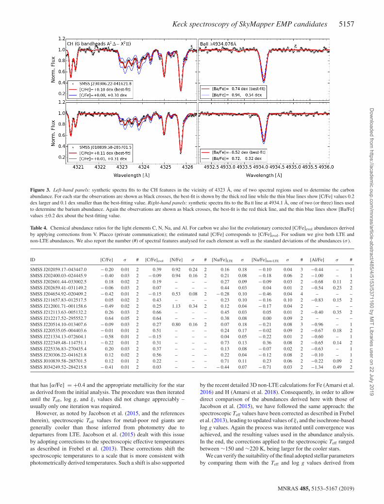
Figure 3. Left-hand panels: synthetic spectra fits to the CH features in the vicinity of 4323 Å, one of two spectral regions used to determine the carbonabundance. For each star the observations are shown as black crosses, the best-fit is shown by the thick red line while the thin blue lines show [C/Fe] values 0.2dex larger and 0.1 dex smaller than the best-fitting value. Right-hand panels: synthetic spectra fits to the Ba II line at 4934.1 Å, one of two (or three) lines usedto determine the barium abundance. Again the observations are shown as black crosses, the best-fit is the red thick line, and the thin blue lines show [Ba/Fe]values ±0.2 dex about the best-fitting value.

Table 4. Chemical abundance ratios for the light elements C, N, Na, and Al. For carbon we also list the evolutionary corrected [C/Fe]evol abundances derivedby applying corrections from V. Placco (private communication); the estimated natal [C/Fe] corresponds to [C/Fe]evol. For sodium we give both LTE andnon-LTE abundances. We also report the number (#) of spectral features analysed for each element as well as the standard deviations of the abundances (σ ).

ID [C/Fe] σ # [C/Fe]evol [N/Fe] σ # [Na/Fe]LTE σ [Na/Fe]non-LTE σ # [Al/Fe] σ #

SMSS J202059.17–043447.0 − 0.20 0.01 2 0.39 0.92 0.24 2 0.16 0.18 − 0.10 0.04 3 −0.44 – 1SMSS J202400.03–024445.9 − 0.40 0.03 2 − 0.09 0.94 0.16 2 0.21 0.08 − 0.18 0.06 2 −1.00 – 1SMSS J202601.44–033002.5 0.18 0.02 2 0.19 – – – 0.27 0.09 − 0.09 0.03 2 −0.68 0.11 2SMSS J202659.41–031149.2 − 0.06 0.03 2 0.07 – – – 0.44 0.03 0.04 0.01 2 −0.54 0.23 2SMSS J204654.92–020409.2 − 0.42 0.01 2 − 0.15 0.53 0.08 2 − 0.28 0.10 − 0.46 0.04 4 – – –SMSS J211657.83–012517.5 0.05 0.02 2 0.43 – – – 0.23 0.10 − 0.16 0.10 2 −0.83 0.15 2SMSS J212001.71–001158.6 − 0.49 0.02 2 0.25 1.13 0.34 2 0.12 0.04 − 0.17 0.04 2 – – –SMSS J212113.63–005132.2 0.26 0.03 2 0.66 – – – 0.45 0.03 0.05 0.01 2 −0.40 0.35 2SMSS J212217.52–295552.7 0.64 0.05 2 0.64 – – – 0.38 0.08 0.00 0.09 2 – – –SMSS J220514.10–013407.6 − 0.09 0.03 2 0.27 0.80 0.16 2 0.07 0.18 − 0.21 0.08 3 −0.96 – 1SMSS J220535.05–004403.6 − 0.01 0.01 2 0.51 – – – 0.24 0.17 − 0.02 0.09 2 −0.67 0.18 2SMSS J221334.13–072604.1 − 0.58 0.01 2 − 0.15 – – – 0.04 0.05 − 0.22 0.01 2 −0.60 – 1SMSS J222349.48–114751.1 − 0.22 0.01 2 0.31 – – – 0.73 0.13 0.36 0.08 2 −0.65 0.14 2SMSS J225336.83–270435.4 0.20 0.03 2 0.37 – – – 0.13 0.08 − 0.07 0.02 2 −0.63 – 1SMSS J230306.22–041621.8 0.12 0.02 2 0.56 – – – 0.22 0.04 − 0.12 0.08 2 −0.10 – 1SMSS J010839.58–285701.5 0.12 0.01 2 0.22 – – – 0.71 0.11 0.23 0.06 2 −0.22 0.09 2SMSS J034249.52–284215.8 − 0.41 0.01 2 0.03 – – – − 0.44 0.07 − 0.71 0.03 2 −1.34 0.49 2

that has [α/Fe] = +0.4 and the appropriate metallicity for the staras derived from the initial analysis. The procedure was then iterateduntil the Teff, log g, and ξ t values did not change appreciably –usually only one iteration was required.

However, as noted by Jacobson et al. (2015, and the referencestherein), spectroscopic Teff values for metal-poor red giants aregenerally cooler than those inferred from photometry due todepartures from LTE. Jacobson et al. (2015) dealt with this issueby adopting corrections to the spectroscopic effective temperaturesas described in Frebel et al. (2013). These corrections shift thespectroscopic temperatures to a scale that is more consistent withphotometrically derived temperatures. Such a shift is also supported

by the recent detailed 3D non-LTE calculations for Fe (Amarsi et al.2016) and H (Amarsi et al. 2018). Consequently, in order to allowdirect comparison of the abundances derived here with those ofJacobson et al. (2015), we have followed the same approach: thespectroscopic Teff values have been corrected as described in Frebelet al. (2013), leading to updated values of ξ t and the isochrone-basedlog g values. Again the process was iterated until convergence wasachieved, and the resulting values used in the abundance analysis.In the end, the corrections applied to the spectroscopic Teff rangedbetween ∼150 and ∼220 K, being larger for the cooler stars.

We can verify the suitability of the final adopted stellar parametersby comparing them with the Teff and log g values derived from

MNRAS 485, 5153–5167 (2019)

Dow

nloaded from https://academ

ic.oup.com/m

nras/article-abstract/485/4/5153/5371160 by MIT Libraries user on 22 July 2019

5158 A. F. Marino et al.

Table 5. Chemical abundances for α elements, Mg, Si, Ca, and Ti. For each element we report the number (#) of analysed spectral features and the resultingstandard deviations (σ ).

ID [Mg/Fe] σ # [Si/Fe] σ # [Ca/Fe] σ # [Ti I/Fe] σ # [Ti II/Fe] σ #

SMSS J202059.17–043447.0 0.40 0.05 3 0.43 0.18 2 0.35 0.19 2 0.10 0.07 6 0.37 0.10 8SMSS J202400.03–024445.9 0.63 0.23 3 0.42 0.01 2 0.58 0.30 2 0.19 0.09 5 0.38 0.13 8SMSS J202601.44–033002.5 0.42 0.01 2 0.57 0.19 2 0.46 – 1 0.45 0.19 2 0.10 0.13 5SMSS J202659.41–031149.2 0.42 0.12 2 0.75 0.32 2 0.39 0.01 2 0.39 0.16 2 0.43 0.17 7SMSS J204654.92–020409.2 0.19 0.16 3 0.18 0.15 2 0.34 0.16 3 − 0.01 0.06 7 0.25 0.12 8SMSS J211657.83–012517.5 0.47 0.07 2 0.56 0.43 2 0.34 0.02 2 0.30 0.15 4 0.03 0.18 8SMSS J212001.71–001158.6 0.36 0.12 2 0.69 0.15 2 0.36 0.07 2 0.20 0.08 5 0.25 0.15 8SMSS J212113.63–005132.2 0.35 0.04 2 0.64 0.46 2 0.33 0.21 2 0.38 0.01 2 0.00 0.15 7SMSS J212217.52–295552.7 0.21 0.09 2 0.87 – 1 – – – – – – − 0.21 0.04 2SMSS J220514.10–013407.6 0.43 0.16 3 0.28 0.33 2 0.37 0.03 2 0.22 0.04 6 0.31 0.13 8SMSS J220535.05–004403.6 0.26 0.19 2 0.72 0.36 2 0.21 – 1 0.28 0.17 2 0.21 0.09 3SMSS J221334.13–072604.1 0.31 0.18 2 0.70 0.03 2 0.38 0.03 2 0.46 0.33 2 0.26 0.17 6SMSS J222349.48–114751.1 0.47 0.00 2 0.60 0.18 2 0.45 – 1 0.43 0.15 2 0.35(1) 0.20 5SMSS J225336.83–270435.4 0.32 0.25 2 0.58 0.14 2 0.48 – 1 – – – 0.03(1) 0.03 2SMSS J230306.22–041621.8 0.48 0.01 2 0.75 0.25 2 0.45 0.03 2 0.32 0.10 5 0.15 0.10 7SMSS J010839.58–285701.5 0.40 0.15 3 0.74 0.27 2 0.43 – 1 0.37 0.11 7 0.34 0.08 6SMSS J034249.52–284215.8 − 0.24 0.06 2 0.11 0.29 2 − 0.08 0.01 2 − 0.28 0.08 4 − 0.20 0.09 8

Notes: (1) Given the lack of Fe II abundances, Fe I has been used for the Ti II abundances relative to Fe.

the spectrophotometric fits to the 2.3 m low-resolution spectra.The comparison is shown in the upper panels of Fig. 2. The toppanel compares the corrected spectroscopic Teff values with thespectrophotometric determinations: it shows excellent agreement– the points scatter about the 1:1 line and the mean differencebetween the determinations is only 10 K (spectroscopic Teff hotter)with a standard deviation of 150 K. Ascribing equal uncertaintiesto each method then indicates that the uncertainty in the adoptedspectroscopic Teff values is of order 100 K. The largest discrepancyoccurs for star SMSS J212217.52–295552.7 where the correctedspectroscopic temperature is ∼450 K hotter than the spectrophoto-metric determination. There is no straightforward explanation forthis difference although we note that, based on the other stars in thesample, the spectrophotometric temperature for this star is too coolby ∼200 K for its (g − i)0 colour. We also note that with g ≈ 16.4,this star is fainter than the usual g = 16 limit for 2.3m follow-upobservations, while the HIRES observations have one of the lowestS/N values in the sample. For consistency of approach we retain theuse of the corrected spectroscopic temperature for this star, althoughthe uncertainty is likely larger than the typical ±100 K value.

The middle panel shows the comparison for the log g values.Here the mean difference, in the sense log g2.3m − log gspec, is+0.05 dex with a standard deviation of 0.35 dex after excludingSMSS J212217.52–295552.7 where the large difference in tem-perature and our isochrone-based approach to fix log gspec, resultsin a significant offset from the spectrophotometric value. Againassuming equal uncertainties in each method, this suggests that theuncertainty in the adopted log g values is of order of ∼0.25 dex.The adopted atmospheric parameters and the resulting [Fe/H]LTE

values are given in Table 2. Together with the [Fe/H]LTE, we list the[Fe/H]non-LTE values obtained by applying non-LTE corrections toFe I lines as in Lind, Bergemann & Asplund (2012) and Lind et al.(2017). For comparison reasons, in the following we will use our[Fe/H]LTE values.

An independent check on the adopted atmospheric parameters isprovided by a comparison with those adopted in Jacobson et al.(2015) for the two stars in common. For SMSS J010839.58–285701.5 we find Teff/log g/[Fe/H]LTE values of 4936/1.86/−2.90,while Jacobson et al. (2015) list 4855/1.55/−3.02. Similarly, forSMSS J034249.52–284215.8 we find 4783/1.58/−2.31 compared

to 4828/1.60/−2.33 in Jacobson et al. (2015). The differences inthe parameters are reassuringly low giving confidence that theresults derived here can be straightforwardly compared with those ofJacobson et al. (2015). We also note that for star SMSS J221334.13–072604.1, Aoki et al. (2013) list parameters of 5150/1.8/−2.55while we find 4810/1.52/−2.89; the higher abundance given by Aokiet al. (2013) is likely largely a direct consequence of the more than300 K higher temperature employed in that study. For completeness,we note that Aoki et al. (2013) did not determine spectroscopictemperatures, rather they used the temperatures determined by theSEGUE Stellar Parameter Pipeline (SSPP) from the SEGUE low-resolution spectra (see Lee et al. 2011 and references therein). Forthis particular star, however, the temperature estimates given (butnot used) by Aoki et al. (2013) from the (V − K)0 and (g − r)0

colours, namely 4724 K and 4867 K, are much more consistentwith our determination of 4810 K than the SSPP value used byAoki et al. (2013).

For completeness we also show in the bottom panel of Fig. 2 acomparison between the [Fe/H]2.3m values estimated from the fits tothe low-resolution spectra and the final [Fe/H]LTE values determinedfrom the analysis of the high-resolution Keck spectra. Given thatthe low-resolution values are quantized at the 0.25 dex level, theagreement is reasonable: the mean difference is 0.33 dex, with thelow-resolution estimates being lower, and the standard deviation ofthe differences is 0.32 dex.

In the following estimates of the internal uncertainties in chem-ical abundances due to the adopted model atmospheres will beestimated by varying the stellar parameters, one at a time, byTeff/log g/[M/H]/ξ t = ±100 K/±0.40 cgs/±0.30 dex/±0.40 km s−1.

3.2 Chemical species analysed

A list of the spectral lines used in the abundance analysis, togetherwith the excitational potentials (E.P.), the total oscillator strengths(log gf) employed, and the measured EWs, is provided in Table 3.The atomic data come from Jacobson et al. (2015), with theexception of a few lines highlighted in Table 3. In most cases theanalysis is based on the measurement of EWs via Gaussian fits to theprofiles of well-isolated lines, as described in Marino et al. (2008);exceptions to this approach are discussed below. When required, and

MNRAS 485, 5153–5167 (2019)

Dow

nloaded from https://academ

ic.oup.com/m

nras/article-abstract/485/4/5153/5371160 by MIT Libraries user on 22 July 2019

Keck spectroscopy of SkyMapper EMP candidates 5159

Tabl

e6.

Che

mic

alab

unda

nces

for

FeI

and

FeII

,and

Fe-p

eak

elem

ents

Sc(S

cII

),C

r,M

n,C

o,N

i,an

dZ

n.Fo

rea

chel

emen

twe

repo

rtth

enu

mbe

r(#

)of

anal

ysed

spec

tral

feat

ures

and

the

resu

lting

rms

(σ).

ID[F

eI/H

]σ

#[F

eII

/H]

σ#

[Sc/

Fe]

σ#

[CrI

/Fe]

σ#

[CrI

I/Fe]

#[M

n/Fe

]σ

#[C

o/Fe

]σ

#[N

i/Fe]

σ#

[Zn/

Fe]

σ#

SMSS

J202

059.

17–0

4344

7.0

−2.3

00.

1738

−2.3

60.

074

0.13

0.35

4−

0.19

0.09

60.

131

−0.2

50.

033

+0.1

00.

166

−0.

02–

10.

060.

022

SMSS

J202

400.

03–0

2444

5.9

−1.9

70.

1936

−1.8

10.

114

0.27

0.32

4−

0.20

0.11

6−0

.01

1−0

.78

0.21

3+0

.28

0.29

6−

0.21

0.01

20.

290.

112

SMSS

J202

601.

44–0

3300

2.5

−2.8

40.

1527

−2.5

40.

122

0.00

–1

0.09

0.20

2–

–−0

.56

0.18

3+0

.36

0.23

6–

––

0.47

–1

SMSS

J202

659.

41–0

3114

9.2

−2.9

40.

1430

−2.8

40.

172

0.41

–1

−0.

120.

153

––

−0.8

40.

033

+0.3

20.

238

––

––

––

SMSS

J204

654.

92–0

2040

9.2

−1.7

10.

1443

−1.6

10.

094

0.10

0.46

4−

0.21

0.09

60.

111

−0.7

40.

083

+0.2

00.

246

−0.

200.

108

0.01

0.01

2SM

SSJ2

1165

7.83

–012

517.

5−2

.56

0.15

29−2

.42

0.07

2–

––

−0.

040.

164

0.17

1−0

.57

0.16

3+0

.21

0.35

50.

18–

1–

––

SMSS

J212

001.

71–0

0115

8.6

−2.5

80.

1638

−2.4

80.

074

0.29

0.23

2−

0.23

0.11

50.

241

−0.5

60.

043

+0.2

10.

374

−0.

17–

10.

420.

032

SMSS

J212

113.

63–0

0513

2.2

−2.7

50.

2135

−2.5

00.

132

0.02

–1

−0.

080.

313

––

−0.5

70.

173

−0.1

10.

154

––

–0.

450.

072

SMSS

J212

217.

52–2

9555

2.7

−2.8

10.

1410

−2.6

2–

1–

––

––

––

–−0

.55

0.11

3–

––

––

––

––

SMSS

J220

514.

10–0

1340

7.6

−2.0

70.

1543

−2.0

20.

074

0.29

0.43

4−

0.15

0.03

60.

221

−0.5

80.

213

+0.4

50.

114

0.06

0.14

60.

220.

072

SMSS

J220

535.

05–0

0440

3.6

−3.1

00.

1829

−3.0

6–

10.

340.

402

−0.

200.

112

––

−0.4

40.

113

+0.1

20.

075

––

––

––

SMSS

J221

334.

13–0

7260

4.1

−2.8

90.

1524

−2.8

0–

1–

––

−0.

100.

132

––

−0.6

90.

153

+0.1

90.

297

––

–0.

59–

1SM

SSJ2

2234

9.48

–114

751.

1−3

.15

0.16

21–

––

––

–−

0.28

–1

––

−1.1

30.

093

+0.1

60.

197

––

––

––

SMSS

J225

336.

83–2

7043

5.4

−3.2

60.

198

––

––

––

––

––

–−1

.05

0.04

3+0

.18

0.36

4–

––

––

–SM

SSJ2

3030

6.22

–041

621.

8−2

.74

0.16

32−2

.53

–1

−0.

14–

1−

0.17

0.03

2–

–−0

.54

0.05

3+0

.28

0.12

7–

––

0.38

–1

SMSS

J010

839.

58–2

8570

1.5

−2.9

00.

1333

−2.9

1–

1–

––

−0.

200.

032

––

−0.5

90.

163

+0.2

40.

229

––

–0.

570.

002

SMSS

J034

249.

52–2

8421

5.8

−2.3

10.

1342

−2.2

10.

064

−0.

41–

1−

0.31

0.11

60.

191

−0.6

20.

053

−0.3

50.

208

−0.

170.

103

––

– when atomic data are available from the literature, hyperfine and/orisotopic splitting was incorporated in the analysis, as indicated inthe last column of Table 3.

We now comment in detail on the transitions used in the analysesfor different element classes, noting that for some species abun-dances are determined only for a subset of the sample depending onthe S/N of the spectrum and the adopted atmospheric parameters.

3.2.1 Light elements

Carbon abundances were derived via spectral synthesis of the CHG-band (A2� − X2�) heads near 4312 and 4323 Å. An oxygenabundance ratio of [O/Fe] = +0.4 dex was assumed as the S/N ofthe spectra does not allow a determination of the oxygen abundancefrom the forbidden [O I] lines at 6300 and 6363 Å. Examples of thesynthetic spectrum fits are shown in the left-hand panels of Fig. 3.Similarly, nitrogen abundances come from spectral synthesis of theCN bands B2� − X2� at ∼3880 and ∼4215 Å, using the carbonabundance derived from the G-band fits. Sodium abundances wereinferred from the Na resonance doublet at ∼5893 Å. For three starswe were able to estimate Na from the doublet ∼5685 Å. Sodiumabundances were then corrected for non-LTE effects, as in Lindet al. (2011), and listed in Table 4. For most stars, we were able toinfer Al abundances from the spectral synthesis of the lines usedalso in Jacobson et al. (2015), namely at ∼3961 and ∼3944 Å.

3.2.2 α-Elements

We determined chemical abundances for the α-elements Mg, Si, Ca,and Ti. For magnesium, silicon, and titanium the abundances couldbe determined for all the stars in the observed sample, since at leastone up to three strong lines were available for these elements; alarger number of lines were generally detectable for Ti, particularlyfor Ti II. Calcium abundances were inferred from only one or twolines (see Table 5).

3.2.3 Iron-peak elements

A few lines were available for each of the iron-peak elements Sc,Cr, Mn, Co, Ni, and Zn (see Table 6). The abundances for theseelements were determined from the measured EWs except for Mnwhere we synthesized the triplet at ≈4033 Å to take into accounthyperfine structure.

3.2.4 Neutron-capture elements

We derived abundances for the neutron-capture elements Sr (fromthe resonance lines 4078,4215 Å), Ba (from the resonance lines4554,4934 Å, and the spectral feature 5854 Å), and Eu (fromthe resonance line 4130 Å). Specifically, we employed a spectrumsynthesis approach to the analysis since hyperfine and/or isotopicsplitting and/or blended features needed to be taken into account.For example, the spectral features of Eu II have both significanthyperfine substructure and isotopic splitting. For this element Solarsystem, isotopic fractions were assumed in the computation. Theright-hand panels of Fig. 3 show examples of the synthetic spectrumfits to the strong Ba II line at 4934.1 Å. Our Ba abundanceswere computed assuming the McWilliam (1998) r-process isotopiccomposition and hyperfine splitting. The derived abundances arelisted in Table 7.

MNRAS 485, 5153–5167 (2019)

Dow

nloaded from https://academ

ic.oup.com/m

nras/article-abstract/485/4/5153/5371160 by MIT Libraries user on 22 July 2019

5160 A. F. Marino et al.

Table 7. Chemical abundances for the n-capture elements, Sr, Ba, and Eu. For each element we report the number (#) of analysed spectral features and theresulting rms (σ ). For some stars we report upper limits.

ID [Sr/Fe] σ # [Ba/Fe] σ # [Eu/Fe] σ #

SMSS J202059.17–043447.0 0.12 0.08 2 − 0.42 0.13 3 − 0.07 – 1SMSS J202400.03–024445.9 0.20 0.29 2 0.05 0.04 3 0.68 0.03 2SMSS J202601.44–033002.5 0.20 0.04 2 − 0.41 0.10 2 <0.80 – –SMSS J202659.41–031149.2 − 1.94 0.06 2 − 1.69 0.00 1 <0.10 – –SMSS J204654.92–020409.2 0.03 0.00 2 − 0.13 0.16 3 0.35 0.19 2SMSS J211657.83–012517.5 − 0.18 0.21 2 − 0.41 0.09 3 0.28 – 1SMSS J212001.71–001158.6 − 0.41 0.07 2 − 0.82 0.15 3 − 0.28 – 1SMSS J212113.63–005132.2 − 0.51 0.01 2 − 1.00 0.02 2 <0.20 – –SMSS J212217.52–295552.7 − 1.15 0.05 2 <− 0.90 0.10 2 <0.80 – –SMSS J220514.10–013407.6 0.03 0.07 2 − 0.38 0.10 3 0.05 – 1SMSS J220535.05–004403.6 − 0.82 0.03 2 − 1.45 0.09 2 <0.30 – –SMSS J221334.13–072604.1 − 0.36 0.04 2 − 1.00 0.09 2 <0.30 – –SMSS J222349.48–114751.1 − 2.00 0.10 2 − 1.63 0.02 2 <0.20 – –SMSS J225336.83–270435.4 − 0.61 0.10 2 − 1.12 0.15 2 <0.90 – –SMSS J230306.22–041621.8 − 0.01 0.01 2 − 0.58 0.10 3 <0.30 – –SMSS J010839.58–285701.5 0.07 0.01 2 − 0.41 0.11 2 <0.30 – –SMSS J034249.52–284215.8 − 0.10 0.01 2 − 0.14 0.10 3 0.55 0.01 2

Table 8. Sensitivity of derived abundances to the uncertainties in atmospheric parameters, the limilted S/N (σ S/N), and the total error due to these contributions(σ tot).

�Teff �log g �ξ t �[A/H] σ S/N σ total

±100 K ±0.40 ±0.40 km s−1 0.30 dex

[C/Fe] ±0.09 −0.10 ±0.05 ±0.11 0.14 0.23[N/Fe] ±0.16 −0.08 ±0.06 −0.20 0.14 0.31[Na/Fe] ±0.01 −0.05 −0.10 −0.01 0.14 0.18[Mg/Fe] −0.06 −0.01 ±0.02 ±0.01 0.14 0.15[Al/Fe] ±0.01 −0.12 −0.10 ±0.03 0.35 0.38[Si/Fe] −0.01 −0.05 −0.03 ±0.01 0.33 0.34[Ca/Fe] −0.05 ±0.01 ±0.04 ±0.01 0.14 0.15[Ti I/Fe] ±0.02 ±0.00 ±0.05 ±0.00 0.10 0.11[Ti II/Fe] ±0.04 −0.01 −0.08 ±0.00 0.08 0.12[Fe I/H] ±0.12 −0.03 −0.08 −0.02 0.04 0.15[Fe II/H] −0.00 ±0.12 −0.03 ±0.02 0.14 0.19[Sc/Fe] ±0.02 −0.04 ±0.01 ±0.00 0.33 0.33[Cr I/Fe] −0.01 ±0.00 ±0.05 ±0.01 0.16 0.17[Cr II/Fe] −0.01 −0.07 ±0.02 −0.01 0.20 0.21[Mn/Fe] ±0.06 −0.07 −0.08 −0.13 0.12 0.21[Co/Fe] ±0.02 −0.03 −0.07 −0.01 0.17 0.19[Ni/Fe] −0.06 ±0.03 ±0.08 ±0.01 0.12 0.16[Zn/Fe] −0.09 ±0.07 ±0.07 ±0.02 0.14 0.19[Sr/Fe] ±0.07 −0.06 −0.22 −0.04 0.14 0.30[Ba/Fe] ±0.07 −0.02 −0.05 −0.02 0.14 0.30[Eu/Fe] ±0.05 ±0.01 ±0.03 ±0.06 0.20 0.22

3.2.5 Abundance errors

Estimates of the uncertainties in the chemical abundances dueto errors in the atmospheric parameteres have been obtained byrerunning the abundances, one at a time, varying Teff/log g/[m/H]/ξ t

by ±100 K/±0.40/±0.30/±0.40 km s−1, assuming that the errorsare symmetric for positive and negative changes. The uncertaintiesused in Teff, log g, and [m/H] are reasonable, as suggested bythe comparison with the spectrophotometric fits to the 2.3 m low-resolution spectra and stars in common with Jacobson et al. (2015)(see Section 3.1). As internal errors in ξ t, we conservatively adopt±0.40 km s−1. The variations in chemical abundances for eachelement are listed in Table 8.

To obtain the total error estimates, we follow the approach byNorris et al. (2010) and Yong et al. (2013). For each element, wereplace the r.m.s (σ ) in Tables 4, 5, 6, and 7 by the maximum(σ ,0.20), where the second term is what would be expected for a set ofN lines (Nlines) with a dispersion of 0.20 dex (a conservative valuefor the abundance dispersion of Fe I lines as listed in Table 6).Then, we derive max(σ , 0.20)/

√Nlines. Typical values obtained

for each element are listed in column (6) of Table 8. The totalerror is obtained by quadratically adding this random error withthe uncertainties introduced by atmospheric parameters. For Sr andBa we conservatively adopt an uncertainty of 0.30 dex, consideringthat the abundances for these elements mostly come from strong

MNRAS 485, 5153–5167 (2019)

Dow

nloaded from https://academ

ic.oup.com/m

nras/article-abstract/485/4/5153/5371160 by MIT Libraries user on 22 July 2019

Keck spectroscopy of SkyMapper EMP candidates 5161

Figure 4. Distribution of the [Fe/H]LTE abundances of our analysed stars(filled-grey histogram) and of the larger sample analysed in Jacobson et al.(2015) (dashed-empty histogram).

resonance lines. Finally, we note that this 1D LTE analysis is subjectto abundance uncertainties from three-dimensional (3D) and non-LTE effects (Asplund 2005).

4 R ESULTS

The distribution of [Fe/H]LTE for the sample of 17 commissioning-era SkyMapper EMP candidates observed at Keck is shown inFig. 4, where it is compared with the [Fe/H]LTE distribution forthe larger sample of 122 commissioning-era SkyMapper EMPcandidates observed at Magellan and analysed in Jacobson et al.(2015). In the Jacobson et al. (2015) sample, one-third of thestars have [Fe/H]LTE < −3.0, while 43 per cent have [Fe/H]LTE

<−2.8 dex. Given the smaller size, the current sample is fullyconsistent with these fractions as ∼20 per cent (3/17) of the starsare found here to have [Fe/H]LTE<−3.0 dex and 47 per cent (8/17)have [Fe/H]LTE <−2.8 dex. The SkyMapper photometric selectiontechnique is therefore clearly quite efficient in selecting metal-poor stars. Indeed, as noted above, using the SkyMapper DR1.1

photometry, ∼40 per cent of the candidates that fall within theselection window shown in Fig. 1, have [Fe/H]2.3m ≤ −2.75 dex. Asa comparison, the similar Northern hemisphere photometric surveyfor EMP stars, Pristine, finds that ∼24 per cent of candidates pho-tometrically selected to have [Fe/H] < −3.0 have spectroscopicallydetermined abundances below [Fe/H] = −3.0 dex (Starkenburget al. 2017). As in Jacobson et al. (2015), we caution againstusing the commissioning-era results to constrain the metallicitydistribution function at low abundances, as the selection biasescannot be reliably established. Future papers based on a much largersample of stars selected from SkyMapper DR1.1 photometry andobserved at low resolution, coupled with an extensive follow-upinvestigation with Magellan, will, however, address this issue.

In the following subsections we consider the abundance trendsamong and between elements of different nucleosynthetic groups.We use as our comparison samples those of Jacobson et al. (2015)and the giant stars in the compilation of Yong et al. (2013), notingthat the parameter determination approaches and the line-lists inthose works are not identical to those used here so that the possibilityof systematic differences cannot be ruled out. Unless otherwisenoted, all abundances and abundance ratios are 1D LTE values.

4.1 Light elements

4.1.1 Carbon

As a star ascends the red giant branch, the envelope expandsinwards, reaching layers affected by CN-cycling, a consequenceof which is a reduction of the carbon abundance in the surfacelayers (and an increase in the surface abundance of N). Since weare interested in the carbon abundance at the star’s birth, the so-called ‘natal’ abundance, our measured carbon abundances needto be corrected for the effects of this evolutionary mixing. Theevolutionary mixing corrections depend on Teff, log g, and [Fe/H]and have been discussed in detail in Placco et al. (2014). Dr. V.Placco (Placco, 2018, private communication) kindly generatedthe appropriate corrections to our observed carbon abundances byassuming a natal [N/Fe] = + 0.0 and applying the Placco et al.(2014) procedure. Table 4 lists the observed [C/Fe] values and the

Figure 5. [C/Fe], corrected for evolutionary mixing effects, as a function of [Fe/H]LTE for our sample of stars, which are shown as black open 5-pointedstar symbols. The left-hand panel shows the comparison of our observed values with the compilation of Placco et al. (2014), shown as grey- and red-filleddiamonds with the latter marking CEMP stars. In the right-hand panel we compare our evolutionary-mixing corrected values with those of Jacobson et al.(2015), plotted as grey-filled circles, that are also corrected for evolutionary-mixing effects. The two stars indicated with blue open circles are the stars withlow neutron-capture elements, as will be discussed in Section 4.4.1.

MNRAS 485, 5153–5167 (2019)

Dow

nloaded from https://academ

ic.oup.com/m

nras/article-abstract/485/4/5153/5371160 by MIT Libraries user on 22 July 2019

5162 A. F. Marino et al.

Figure 6. Nitrogen, sodium, and aluminum abundance ratios, relative to iron, as a function of [Fe/H]LTE. The [N/Fe] abundances are compared with the sampleof Yong et al. (2013) in the upper-left panel where upper limits on the [N/Fe] values are shown as downward-pointing arrows. The LTE [Na/Fe] abundanceratios derived here are compared with the Yong et al. (2013) values in the middle-left panel (symbols as for the upper-left panel), and with the Jacobson et al.(2015) sample in the middle-right panel. In the middle-right panel we also show, as blue-filled stars, our [Na/Fe] values corrected for non-LTE (NLTE) effects.These lie at lower values and are connected to the corresponding LTE points by thin blue lines. Aluminum abundances are compared with the Yong et al.(2013) and the Jacobson et al. (2015) in the lower-left and lower-right panels, respectively. The two stars indicated with blue open circles are the stars with lowneutron-capture elements, as will be discussed in Section 4.4.1.

correction for evolutionary mixing: the estimated ‘natal’ [C/Fe] isformed by adding the correction to the observed value.

In Fig. 5 we show in the left-hand panel a comparison of ourobserved [C/Fe] values with those listed in Placco et al. (2014),which are corrected for evolutionary-mixing effects. The right-handpanel shows the comparison of our [C/Fe] values, after applyingthe evolutionary mixing corrections, with the evolutionary mixingcorrected values of Jacobson et al. (2015). Placco et al. (2014)have demonstrated that the fraction of carbon-enhanced metal-poor(CEMP) stars, defined as stars possessing [C/Fe] ≥ +0.7 dex,increases with decreasing metallicity with CEMP stars dominantbelow [Fe/H] ≤ −4.0 (see also Yoon et al. 2016, 2018). ThePlacco et al. (2014) CEMP frequencies (e.g. ∼40 per cent for[Fe/H] ≤ −3.0) would suggest that our sample of three starswith [Fe/H]LTE ≤ −3.0 should contain one CEMP-star whereasthere are none. While the statistical weight of the lack of CEMP-stars compared to the number expected is not high, inspectionof Fig. 5 reveals that none of our sample of 17 stars has a[C/Fe] value that would cause it to be classified as CEMP-star:the highest evolutionary corrected [C/Fe] values are 0.66 dex forSMSS J212113.63–005132.2 ([Fe/H]LTE = −2.74) and 0.64 dex

for SMSS J212217.52–295552.7 ([Fe/H]LTE = −2.81). In general,our evolutionary mixing corrected [C/Fe] values are completelyconsistent with those from the larger sample of Jacobson et al.(2015). Jacobson et al. (2015) discussed the frequency of CEMP-stars in their sample and concluded that it is comparable with thatof Placco et al. (2014) although, as is evident in Fig. 5, the Jacobsonet al. (2015) sample lacks CEMP-stars with [C/Fe] significantlyabove 1.0.

The most likely explanation lies in the selection of EMP candi-dates from the SkyMapper photometry. As discussed in Da Costaet al. (), the strong CH bands in the spectrum of a CEMP-starcan depress the flux in the SkyMapper v-filter sufficiently that theinferred metallicity index mimics a more metal-rich star, and thusdecreases the probability that it will be selected for low-resolutionspectroscopic follow-up. Nevertheless the commissioning surveydid result in the discovery of the most iron-poor star currentlyknown, a star that is extremely C-rich (Keller et al. 2014; Bessellet al. 2015; Nordlander et al. 2017). Evidently at sufficiently lowoverall abundance the contaminating carbon features in the v bandweaken enough that selection as a photometric candidate againbecomes possible.

MNRAS 485, 5153–5167 (2019)

Dow

nloaded from https://academ

ic.oup.com/m

nras/article-abstract/485/4/5153/5371160 by MIT Libraries user on 22 July 2019

Keck spectroscopy of SkyMapper EMP candidates 5163

Figure 7. Chemical abundance ratios with respect to Fe for the α-elements measured in this study as a function of [Fe/H]LTE. The 5-point star symbols are thestars in the current sample, while the grey solid circles are stars from Yong et al. (2013, left-hand panels) and Jacobson et al. (2015, right-hand panels). Thetwo stars indicated with blue open circles are the stars with low neutron-capture elements, as will be discussed in Section 4.4.1.

4.1.2 Nitrogen, sodium, and aluminum

The nitrogen, sodium, and aluminum abundance ratios with respectto iron for our sample are shown in Fig. 6 as a function of [Fe/H]LTE.Because of low S/N at the wavelength of the CN bands in many ofthe spectra, [N/Fe] values could be determined only for five stars inour sample. The values, which lie between 0.5 and ∼1.0, and whichare listed in Table 4, are nevertheless consistent with the midpointof the substantial range of [N/Fe] values found in the sample ofYong et al. (2013).

For sodium, while noting that the non-LTE corrections wouldresult in lower abundance ratios, we have plotted the LTE abundanceratios to facilitate comparison with the Yong et al. ( 2013) andJacobson et al. (2015) samples. In the comparison plot withJacobson et al. (2015) we have also plotted our non-LTE-correctedvalues of Na (Lind et al. 2011), to highlight the general lowerabundances for this element that would be obtained with a propernon-LTE analysis. It is clear from the panels of Fig. 6 that our resultsfor [Na/Fe] are generally consistent with those of the earlier studies.The one possible exception is the star SMSS J034249.52–284215.8,which has [Na/Fe]LTE of −0.44 and [Fe/H]LTE = −2.31 dex. Sucha low [Na/Fe] is reminiscent of the low [Na/Fe] values seen inred giant members of dwarf Spheroidal galaxies (e.g. Geisler et al.

2005; Hasselquist et al. 2017; Norris et al. 2017, and referencestherein). The low value for [Na/Fe] found here is consistent withthat listed by Jacobson et al. (2015): [Na/Fe]LTE = −0.29, thelowest [Na/Fe]LTE in their entire sample. We give both the LTE andnon-LTE [Na/Fe] values for our stars in Table 4.

Aluminum abundance ratios of our sample are comparable to boththose of Yong et al. (2013) and Jacobson et al. (2015) (lower panelsof Fig. 6). We note that the uncertainties associated with our [Al/Fe]values are large due to the relatively low S/N of our spectra, espe-cially below 4000 Å. As for [Na/Fe] we expect the application ofnon-LTE corrections to generate systematic offsets in the [Al/Fe]LTE

values; such corrections can be as large as +0.65 dex (Baumueller &Gehren 1997). As discussed in the previous work, such higher non-LTE [Al/Fe] abundances would be more consistent with predictionsof chemical evolution models (e.g. Kobayashi et al. 2006).

4.2 α-Elements

The individual α-element (Mg, Si, Ca, Ti I, Ti II) abundances forour sample are displayed as a function of [Fe/H]LTE in Fig. 7 andlisted in Table 5. With the exception of one star, all our stars areα-enhanced and their location in the [element/Fe] panels is fullyconsistent with the larger comparison samples of Jacobson et al.(2015) and Yong et al. (2013).

MNRAS 485, 5153–5167 (2019)

Dow

nloaded from https://academ

ic.oup.com/m

nras/article-abstract/485/4/5153/5371160 by MIT Libraries user on 22 July 2019

5164 A. F. Marino et al.

Figure 8. Chemical abundance ratios with respect to Fe for the iron-peak elements as a function of [Fe/H]LTE. Symbols are as in Fig. 7. The left-hand panelsshow the comparison with the results of Yong et al. (2013), while the right-hand panels show the comparison with Jacobson et al. (2015). The two starsindicated with blue open circles are the stars with low neutron-capture elements, as will be discussed in Section 4.4.1.

The one star that does not show any α-enhancement is thestar SMSS J034249.52–284215.8, which was identified as a ‘Fe-enhanced’ star in Jacobson et al. (2015, specifically Section 5.1). Forthis star we find ([Mg/Fe], [Si/Fe], [Ca/Fe], [Ti/Fe] I and [Ti/Fe] II)values of (−0.24, +0.11, −0.08, −0.28, −0.20), values that arefully consistent with those of Jacobson et al. (2015), which are(−0.17, +0.14, −0.16, −0.37, −0.13). We find also that the otherelements analysed in this star generally have sub-solar ratios, againconsistent with Jacobson et al. (2015). We note that in Section 3.1we have used α-enhanced isochrones for all the stars. A solar-scaled[α/Fe] isochrone, more appropriate for this star, results in a lowerlog g by ∼0.10 dex, which does not significantly affect the derivedabundances relative to Fe (see Table 8).

Discussion of the possible origin(s) of this star is given inJacobson et al. (2015). We only note that as mentioned above, thelow [Na/Fe] for this star, plus its ‘alpha-poor’ nature, is reminiscentof abundance ratios seen in dSph stars. The kinematics of the starare not unusual in comparison with those for the rest of the sample.

This star also has the lowest [Al/Fe] in both our sample and that ofJacobson et al. (2015).

4.3 Fe-peak elements

In Fig. 8 we show our results for the abundance ratios with respectto iron for the iron-peak elements Sc, Cr I, Cr II, Mn, Co, Ni, and Znas a function of [Fe/H]LTE. The values are listed in Table 6 alongwith both the number of spectral features analysed and the standarddeviations (σ ). Also shown in the panels are the equivalent data,where available, for the stars in the comparison samples of Yonget al. (2013) and Jacobson et al. (2015). Although our sample is notlarge compared to the others, it is evident from the figure that ourresults are consistent with the abundance ratio trends seen in thecomparison samples. There is, however, a suggestion that the Keckdata presented here have some systematic differences relative to thecomparison samples. For example, although the Keck stars show thesame rate of increase in [Zn/Fe] with decreasing [Fe/H]LTE as the

MNRAS 485, 5153–5167 (2019)

Dow

nloaded from https://academ

ic.oup.com/m

nras/article-abstract/485/4/5153/5371160 by MIT Libraries user on 22 July 2019

Keck spectroscopy of SkyMapper EMP candidates 5165

Figure 9. Upper panels: Chemical abundance ratios with respect to Fe for the neutron-capture elements Sr and Ba as a function of [Fe/H]LTE. Lower panels:[Sr/Ba] as a function of [Ba/Fe]. We compare our results with data from Yong et al. (2013) in the left-hand panels and with Jacobson et al. (2015) in theright-hand panels. Symbols are as in Fig. 5. The two stars indicated with blue open circles are the stars with low neutron-capture elements.

stars in the Jacobson et al. (2015) sample, there might be an offsetin that the current sample have [Zn/Fe] abundance ratios ∼0.2 dexhigher than the Jacobson et al. (2015) values at similar [Fe/H]. Thestar observed here that is in common with Jacobson et al. (2015) isconsistent with this offset.

4.4 n-Capture elements

4.4.1 Strontium and barium

Among the n-capture elements, those that could be analysed in thespectra of the majority of the stars observed here are Sr and Ba.As regards the s-process, Sr is a first s-process peak element whileBa occurs in the second s-process peak. Both can be generatedby the 22Ne or the 13C neutron source depending on the neutronexposure. These elements can also have r-process contributions andthus the relative abundances of these elements in metal-poor starscan provide information on nucleosynthetic processes at early times.

The abundance ratios [Sr/Fe] and [Ba/Fe] for the stars in oursample are shown as a function of [Fe/H]LTE in the upper and middlepanels of Fig. 9 and are listed in Table 7. We note first that none ofour stars show high (>1 dex) abundance ratios for these elements,i.e. none can be classified as s-enhanced stars. This is consistent withthe lack of CEMP-stars in our sample, as discussed in Section 4.1.As is also apparent in the panels of Fig. 9, our results are generallyconsistent with those of Yong et al. (2013), which include CEMP-s stars, and Jacobson et al. (2015). There is some indication that

perhaps our [Sr/Fe] values are systemically lower than those ofJacobson et al. (2015), by approximately 0.3 dex, which is howeverwithin our observational uncertainties (see Table 8).

It is well-known that as overall abundance decreases, the disper-sion in the abundance ratios for the n-capture elements relative toiron increases markedly (e.g. McWilliam et al. 1995; Frebel & Nor-ris 2015, and references therein), undoubtedly reflecting variationsin the relative contributions of the numerous nucleosynthetic originsfor these elements. This is illustrated in the lower panels of Fig. 9,where we show the [Sr/Ba] ratio as a function of [Ba/Fe], includingCEMP-s stars. Concentrating on the stars without s-enhancements,i.e. those with [Ba/Fe] ≤ 0.0 approximately, we see that the rangein [Sr/Ba] increases substantially as [Ba/Fe] decreases reachingalmost two orders of magnitude at the lowest [Ba/Fe] values. Thedata suggest that the upper limit on [Sr/Ba] increases as [Ba/Fe]decreases, whereas the lower limit appears approximately constantwith decreasing [Ba/Fe]. The Solar system r-process pattern has[Sr/Ba] = −0.5 dex, though lower values are seen in some ultra-faint dwarf galaxy member stars (see Frebel & Norris 2015 andreferences therein) and do occur in both the Yong et al. (2013) andJacobson et al. (2015) data sets.

Casey & Schlaufman (2017) found a star with [Ba/Fe] ∼ −3,with typical main r-process abundance patterns, a signature ofthe universality of the r-process. Six stars with very low [Ba/Fe]([Ba/Fe]<−1.5) but which show a range of [Sr/Ba] of ∼2 dexwere identified by Jacobson et al. (2015). One of these stars has[Sr/Ba] ≈ −0.5, i.e. the Solar system r-process value, with an upper

MNRAS 485, 5153–5167 (2019)

Dow

nloaded from https://academ

ic.oup.com/m

nras/article-abstract/485/4/5153/5371160 by MIT Libraries user on 22 July 2019

5166 A. F. Marino et al.

Figure 10. Upper panel: [Eu/Fe] as a function of [Fe/H]LTE for our samplecompared with the Jacobson et al. (2015) sample. In both cases upper limitson [Eu/Fe] are indicated by downward pointing arrows. The dashed lines are[Eu/Fe] = +0.3 and [Eu/Fe] = +1 show the classification values for r-I andr-II stars, respectively. The two stars indicated with blue open circles arethe two stars with the lowest neutron-capture element abundances. Lowerpanel: [Ba/Eu] as a function of [Fe/H]LTE for the stars with measured Euabundances or upper limits. Symbols are as in the upper panel. The fouropen circles in the Jacobson et al. (2015) sample are the stars with upperlimits in both Ba and Eu. One star in our sample also has only upper limitsand has been represented with a small star-like symbol, without upwardlimit. The black dashed line and the grey dotted-dashed line are the mean[Ba/Eu] abundances in our sample and Jacobson et al. (2015), respectively.The size of the y-axis has been kept the same as in the upper panel.

limit on [Eu/Fe] of ∼0.4 dex. It is therefore strongly depleted inn-capture elements. We have identified two similar stars in our sam-ple: SMSS J202659.41–031149.2 for which [Fe/H]LTE = −2.94,[Ba/Fe] = −1.69 and [Sr/Ba] = −0.25, and SMSS J222349.48–114751.1 for which the corresponding values are −3.15, −1.63,and −0.37 dex. Neither star has a detectable Eu II line at 4129 Åyielding an approximate upper limit of [Eu/Fe] ≈ 0.10–0.20 dex.Detailed abundances for other n-capture elements for these starswould provide important information on n-capture nucleosynthesisprocesses at early times, e.g. the weak r-process versus the mainr-process (e.g. Roederer 2013; Li et al. 2015b).

4.4.2 Europium

Europium is predominantly synthesized by the r-process (e.g.Sneden, Cowan & Gallino 2008) and as such, the [Eu/Fe] abundanceratio is used to identify r-processed enhanced stars: r-II stars have[Eu/Fe] ≥ + 1.0 while the more moderately enhanced r-I stars have0.3 ≤ [Eu/Fe] ≤ 1.0 dex. Both types have [Ba/Eu] < 0 (Barklem

et al. 2005). We have measured Eu abundances for as many ofthe stars in our sample as possible, and derived upper limits for theothers. The results are shown in the upper panel of Fig. 10, where wecompare our results with those of Jacobson et al. (2015) (we note thatYong et al. 2013 did not determine Eu abundances). The agreementis reasonable. The [Eu/Fe] determinations are also given in Table 7.Overall, the scatter in the [Eu/Fe] values is comparable to that seenin Jacobson et al. (2015) and to that in the literature compilationof Frebel (2010). One star in our sample, SMSS J202400.03–024445.9, is a probable r-I star – for this star, which has [Fe/H]LTE

= −1.95, we find [Eu/Fe] = +0.68 and [Ba/Eu] = −0.63 dex.Star SMSS J034249.52–284215.8, which we have already drawnattention to because of its low values of [α/Fe] and [Na/Fe], andwhich is the ‘Fe-enhanced’ star discussed in Jacobson et al. (2015),is also a candidate r-I star. It has [Fe/H]LTE = −2.31, [Eu/Fe]= +0.55, and [Ba/Eu] = −0.67 dex. Star SMSS J204654.92–020409.2 also just meets the r-I classification with [Fe/H]LTE =−1.70, [Eu/Fe] = +0.35, and [Ba/Eu] = −0.48 dex. Indeed the[Ba/Eu] abundance ratio in all three stars is consistent with thescaled-solar r-process value. The lower panel of Fig. 10 shows theabundance ratio [Ba/Eu] as a function of [Fe/H]LTE. The average[Ba/Eu] for all the seven stars with both Ba and Eu measurementsis −0.54, close to the scaled-solar r-process value. We note thatfor these stars, the standard deviations of the [Ba/Fe] and [Eu/Fe]values are 0.28 and 0.34 dex, respectively. However, the standarddeviation of the [Ba/Eu] ratio for these stars is substantially less at0.13 dex. This may indicate that while the total production of Baand Eu is variable, the nucleosynthetic site(s) involved produce Baand Eu in very similar relative amounts.

5 SU M M A RY

We have presented here the results of an analysis of high-resolutionspectra, obtained with the Keck telescope and the HIRES spec-trograph, of 17 candidate EMP stars selected from SkyMappercommissioning-era photometry. Fourteen of the stars had notpreviously been observed at high dispersion. We find that, asin Jacobson et al. (2015), the candidate selection process, i.e.photometry plus low-resolution spectroscopy, is robust with almosthalf of the sample having [Fe/H]LTE ≤ −2.8 and with only one‘false positive’ – an EMP candidate for which [Fe/H] turned outto exceed [Fe/H]LTE = −2.0 dex. In general, the distribution ofelement abundances and abundance ratios for this sample closelymimics the earlier results of Jacobson et al. (2015) that was based onMagellan/MIKE high-dispersion spectroscopy of a large sample ofSkyMapper commissioning-era EMP candidates. Specifically, wefind that none of the present sample can be classified as CEMP stars.Further, we confirm the results of Jacobson et al. (2015) that thestar SMSS J034249.52–284215.8 is an example of the relativelyrare class of objects known as ‘Fe-enhanced’ stars – stars withgenerally sub-solar abundance ratios, including for the α-elements.The star may have originated in a dwarf spheriodal galaxy. Twofurther stars, SMSS J202659.41–031149.2 and SMSS J222349.48–114751.1, are found to be strongly depleted in n-capture elements:[Ba/Fe]<−1.6, [Sr/Ba] ≈ −0.3 dex, and [Eu/Fe] � +0.10–0.15joining the similar star identified in Jacobson et al. (2015), whilethe star SMSS J202400.03–024445.9 is a probable r-I star with[Eu/Fe] = +0.68, [Ba/Eu] = −0.63, and [Fe/H]LTE = −1.95 dex.

AC K N OW L E D G E M E N T S

We thank the anonymous referee for his or her suggestions thatimproved the manuscript. We thank Dr Vini Placco for providing the

MNRAS 485, 5153–5167 (2019)

Dow

nloaded from https://academ

ic.oup.com/m

nras/article-abstract/485/4/5153/5371160 by MIT Libraries user on 22 July 2019

Keck spectroscopy of SkyMapper EMP candidates 5167

evolutionary mixing corrections to the observed carbon abundances.SkyMapper research on EMP stars has been supported in partthrough the Australian Research Council (ARC) Discovery Grantprograms DP120101237 and DP150103294 (Lead-CI Da Costa).A. F. M., A. R. C., and A. D. M. have been in part supportedby ARC through the Discovery Early Career Researcher AwardDE160100851, the Discovery Project DP160100637, and the FutureFellowship FT160100206, respectively. M. A. gratefully acknowl-edges generous funding from an ARC Laureate Fellowship (grantFL110100012). Parts of this research were conducted under theauspices of the Australian Research Council Centre of Excellencefor All Sky Astrophysics in 3 Dimensions (ASTRO 3D), whichis supported through project number CE170100013. This projecthas received funding from the European Union’s Horizon 2020research and innovation programme under the Marie Skłodowska-Curie Grant Agreement No. (797100; Beneficiary: A. F. M.).

The national facility capability for SkyMapper has been fundedthrough ARC LIEF grant LE130100104 from the Australian Re-search Council, awarded to the University of Sydney, the AustralianNational University, Swinburne University of Technology, theUniversity of Queensland, the University of Western Australia,the University of Melbourne, Curtin University of Technology,Monash University, and the Australian Astronomical Observatory.SkyMapper is owned and operated by The Australian NationalUniversity’s Research School of Astronomy and Astrophysics. Thesurvey data were processed and provided by the SkyMapper Teamat ANU. The SkyMapper node of the All-Sky Virtual Observatory(ASVO) is hosted at the National Computational Infrastructure(NCI). Development and support the SkyMapper node of the ASVOhave been funded in part by Astronomy Australia Limited (AAL)and the Australian Government through the Commonwealth’sEducation Investment Fund (EIF) and National Collaborative Re-search Infrastructure Strategy (NCRIS), particularly the NationaleResearch Collaboration Tools and Resources (NeCTAR), and theAustralian National Data Service Projects (ANDS).

The high dispersion spectra presented herein were obtained at theW.M. Keck Observatory, which is operated as a scientific partner-ship among the California Institute of Technology, the University ofCalifornia, and the National Aeronautics and Space Administration.The Observatory was made possible by the generous financialsupport of the W.M. Keck Foundation.

The authors wish to recognize and acknowledge the very sig-nificant cultural role and reverence that the summit of Mauna Keahas always had within the indigenous Hawaiian community. We aremost fortunate to have the opportunity to conduct observations fromthis mountain.

We also acknowledge the traditional owners of the land on whichthe SkyMapper telescope stands, the Gamilaraay people, and payour respects to elders past and present.

REFERENCES

Amarsi A. M., Lind K., Asplund M., Barklem P. S., Collet R., 2016,MNRAS, 463, 1518

Amarsi A. M., Nordlander T., Barklem P. S., Asplund M., Collet R., LindK., 2018, A&A, 615, A139

Aoki W. et al., 2013, AJ, 145, 13Asplund M., 2005, ARA&A, 43, 481Asplund M., Grevesse N., Sauval A. J., Scott P., 2009, ARA&A, 47, 481Barklem P. S. et al., 2005, A&A, 439, 129Baumueller D., Gehren T., 1997, A&A, 325, 1088Beers T. C., Preston G. W., Shectman S. A., 1992, AJ, 103, 1987Bessell M. S. et al., 2015, ApJ, 806, L16

Bessell M., Bloxham G., Schmidt B., Keller S., Tisserand P., Francis P.,2011, PASP, 123, 789

Casey A. R., Schlaufman K. C., 2017, ApJ, 850, 179Castelli F., Kurucz R. A., 2004, preprint (astro-ph/0405087)Christlieb N., Schorck T., Frebel A., Beers T. C., Wisotzki L., Reimers D.,

2008, A&A, 484, 721Demarque P., Woo J.-H., Kim Y.-C., Yi S. K., 2004, ApJS, 155, 667Dopita M. A. et al., 2010, Ap&SS, 327, 245Frebel A., 2010, Astron. Nachr., 331, 474Frebel A., Norris J. E., 2015, ARA&A, 53, 631Frebel A. et al., 2006, ApJ, 652, 1585Frebel A., Casey A. R., Jacobson H. R., Yu Q., 2013, ApJ, 769, 57Gaia Collaboration, 2018, A&A, 616, A1Geisler D., Smith V. V., Wallerstein G., Gonzalez G., Charbonnel C., 2005,

AJ, 129, 1428Hasselquist S. et al., 2017, ApJ, 845, 162Howes L. M. et al., 2015, Nature, 527, 484Howes L. M. et al., 2016, MNRAS, 460, 884Jacobson H. R. et al., 2015, ApJ, 807, 171Keller S. C. et al., 2007, Publ. Astron. Soc. Aust., 24, 1Keller S. C. et al., 2014, Nature, 506, 463Kobayashi C., Umeda H., Nomoto K., Tominaga N., Ohkubo T., 2006, ApJ,

653, 1145Lee Y. S. et al., 2011, AJ, 141, 90Li H., Aoki W., Zhao G. et al., 2015a, PASJ, 67, 84Li H.-N. et al., 2015b, ApJ, 798, 110Lind K., Asplund M., Barklem P. S., Belyaev A. K., 2011, A&A, 528, A103Lind K., Bergemann M., Asplund M., 2012, MNRAS, 427, 50Lind K. et al., 2017, MNRAS, 468, 4311Marino A. F., Villanova S., Piotto G., Milone A. P., Momany Y., Bedin L.

R., Medling A. M., 2008, A&A, 490, 625McWilliam A., 1998, AJ, 115, 1640McWilliam A., Preston G. W., Sneden C., Searle L., 1995, AJ, 109, 2757Nordlander T., Amarsi A. M., Lind K., Asplund M., Barklem P. S., Casey

A. R., Collet R., Leenaarts J., 2017, A&A, 597, A6Norris J. E. et al., 2013, ApJ, 762, 25Norris J. E., Yong D., Venn K. A., Gilmore G., Casagrande L., Dotter A.,

2017, ApJS, 230, 28Norris J. E., Yong D., Gilmore G., Wyse R. F. G., 2010, ApJ, 711, 350Placco V. M., Frebel A., Beers T. C., Stancliffe R. J., 2014, ApJ, 797, 21Roederer I. U., 2013, AJ, 145, 26Schlaufman K. C., Casey A. R., 2014, ApJ, 797, 13Sneden C. A., 1973, PhD thesis, Univ. TexasSneden C., Cowan J. J., Gallino R., 2008, ARA&A, 46, 241Starkenburg E. et al., 2017, MNRAS, 471, 2587VandenBerg D. A., Bergbusch P. A., Dowler P. D., 2006, ApJS, 162, 375Vogt S. S. et al., 1994, Proc. SPIE Conf. Ser. Vol. 2198 , HIRES: the high-

resolution echelle spectrometer on the Keck 10-m Telescope, SPIE,Bellingham, p. 362

Wolf C. et al., 2018, PASA, 35, 10Wolf C. et al., 2018, Publ. Astron. Soc. Aust., 35, e010Yong D. et al., 2013, ApJ, 762, 26Yoon J. et al., 2016, ApJ, 833, 20Yoon J. et al., 2018, ApJ, 861, 146

SUPPORTI NG INFORMATI ON

Supplementary data are available at MNRAS online.

linelist paper.tex

Please note: Oxford University Press is not responsible for thecontent or functionality of any supporting materials supplied bythe authors. Any queries (other than missing material) should bedirected to the corresponding author for the article.

This paper has been typeset from a TEX/LATEX file prepared by the author.

MNRAS 485, 5153–5167 (2019)

Dow

nloaded from https://academ

ic.oup.com/m

nras/article-abstract/485/4/5153/5371160 by MIT Libraries user on 22 July 2019