Companies in energy markets employ a wide variety of trading and hedging strategies for their power stations. All strategies basically stem from the wish to maximise profit or minimise risk, or both. In this article we explain

the logic of several such strategies and compare various ways of implementation these for gas and coal-fired power stations. We focus in particular on the delta-hedging strategy and ways to calculate deltas. One of our findings is that simple formulas to calculate delta hedges lead to severe biases in risk reporting and portfolio management. However, this does not need to be so, as relatively quick

calculation methods exist to come up with more accurate figures. Hedging means trading in a market in order to reduce risk on an

existing position. In the context of a power station, hedging comes down to selling power forward and buying fuels and carbon credits forward, so as to avoid the spot markets. The hedging transactions can be placed in tradable contracts (forwards, futures, swaps) or can be in the form of structured contracts, such as power purchasing agreements (PPAs) and long-term gas contracts (swing or take-or-pay contracts). Entering into such contracts will generally reduce risk but might be necessary due to the limited liquidity (or absence) of spot markets.

A comparison of common delta hedging strategies and calculations finds that simple formulas used to calculate delta hedges can lead to severe biases. Cyriel de Jong, Hans van Dijken and Alexandra Bundalova suggest a relatively fast, but more accurate calculation method

64 risk.net/energy-risk November 2011

Power plant hedging strategies

Dm

itry

Na

um

ov /

Sh

utt

erst

ock.

com

Keeping your options open

November 2011 risk.net/energy-risk 65

Power plant hedging strategies

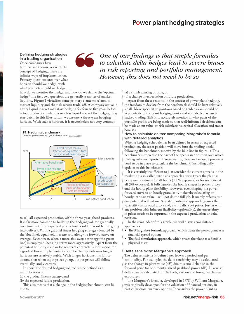
Defi ning hedging strategies in a trading organisation Once companies have familiarised themselves with the concept of hedging, there are infi nite ways of implementation. Primary questions are: over what horizon should we hedge, with what products should we hedge, how do we monitor the hedge, and how do we defi ne the ‘optimal’ hedge? Th e fi rst two questions are generally a matter of market liquidity. Figure 1 visualises some primary elements related to market liquidity and the risk-return trade-off . A company active in a very liquid market may start hedging for four to fi ve years before actual production, whereas in a less liquid market the hedging may start later. In this illustration, we assume a three-year hedging horizon. With such a horizon, it is nevertheless not very common

to sell all expected production within three-year-ahead products. It is far more common to build up the hedging volume gradually over time until the expected production is sold forward before going into delivery. With a gradual linear hedging strategy (denoted by the blue line), equal volumes are sold along the forward curve on average. By contrast, when a more-risk averse strategy (the green line) is employed, hedging starts more aggressively. Apart from the potential liquidity issue in longer-term contracts, a motivation for a gradual linear implementation can be that spreads over longer horizons are relatively stable. With longer horizons it is fair to assume that when input prices go up, output prices will follow eventually, and vice versa.

In short, the desired hedging volume can be defi ned as a multiplication of (a) the gradual linear strategy; and (b) the expected future production.

Th is also means that a change in the hedging benchmark can be due to:

(a) a simple passing of time; or (b) a change in expectation of future production.

Apart from these reasons, in the context of power plant hedging, the freedom to deviate from the benchmark should be kept relatively small. More speculative positions based on trader views should be kept outside of the plant hedging books and not labelled as asset-backed trading. Th is is to accurately monitor in what parts of the portfolio profi ts are being made so that well-informed decisions can be made about value-at-risk calculations, capital allocation and trader bonuses. How to calculate deltas: comparing Margrabe’s formula with detailed analyticsWhen a hedging schedule has been defi ned in terms of expected production, the asset position will move into the trading books following the benchmark (shown by the blue line in fi gure 1). Th is benchmark is then also the part of the open-asset position over which trading risks are reported. Consequently, clear and accurate processes need to be in place to calculate the benchmark, including daily updates to this benchmark.

It is certainly insuffi cient to just consider the current spreads in the market: this so-called intrinsic approach always treats the plant as being in-the-money for all hours (100% exposure) or for no hours at all (0% exposure). It fully ignores the hourly shapes in power prices and the hourly plant fl exibility. However, even shaping the power forward curve to an hourly granularity – thereby calculating an hourly intrinsic value – will not do the full job. It merely refl ects just one potential realisation. Any static intrinsic approach ignores the variability in forward prices and, eventually, spot prices. Just as with any position with inherent fl exibility (optionality), the uncertainty in prices needs to be captured in the expected production or delta position.

In the remainder of this article, we will discuss two distinct approaches: • Th e Margrabe’s formula approach, which treats the power plant as a

fi nancial spread option;• Th e full-simulation approach, which treats the plant as a fl exible

physical asset.

Delta sensitivity: Margrabe’s approachTh e delta sensitivity is defi ned per forward period and per commodity. For example, the delta sensitivity may be calculated as the change in plant value (dV) due to a small change in the forward price for one-month-ahead peakload power (dP). Likewise, deltas can be calculated for the fuels, carbon and foreign exchange exposures.

Th e Margrabe’s formula, developed in 1978 by William Margrabe, was originally developed for the valuation of fi nancial options, in particular cross-currency options. It considers the power plant as

Time before production-1-2

Fixed benchmark =fraction of expected futureproduction (linear dripping)

Flexibility of tradeposition to deviatefrom benchmark

Max capacity

-3

MW

Expectedproduction =delta position

Alternative benchmark=

lower price risk butmore liquidity risk

F1. Hedging benchmarkDeltahedgeimplementedgraduallyovertimeSource: KYOS

One of our fi ndings is that simple formulas to calculate delta hedges lead to severe biases in risk reporting and portfolio management. However, this does not need to be so

66 risk.net/energy-risk November 2011

Power plant hedging strategies

being a call option to produce power by consuming fuel and carbon credits. It takes the spread between the power price and the ‘fuel plus carbon’ price as the underlying commodity. The formula yields both the option value and the two delta sensitivities in closed-form. We take a gas-fired power station as an example, assuming 50% lower heating value efficiency. The efficiency implies 2 megawatt hours (MWh) of gas are needed to produce 1 MWh of power. Together with a carbon content of 0.22 ton/MWh of gas, the spark spread and the spark spread option are defined as follows:

Spark spread power price gas price -

2 0.22

=

∗

∗ ∗

-2

CCO priceSpark spread option spark spread,

2

= max 00( )

The option reflects the principle that the plant is only dispatched when the spark spread is positive, so only then it generates a pay-off, equal to this same spark spread.

The Margrabe’s formula requires the current forward price levels of the underlying spread as an input, where the spread consists of only two commodities. In the case of the carbon markets, this means that we need to treat the fuel plus carbon price as a single commodity. In our example, the second leg equals twice the forward price of gas plus 0.44 times the forward price of carbon. For the direct application of Margrabe’s formula, we have to assume that this second leg follows a Geometric Brownian Motion (GBM) process.

The major issue in the application of the Margrabe’s formula is treatment of the flexibility and constraints. There are basically two potential approaches to remedy this:• On the one extreme, the plant can be considered a strip of hourly

call options, which can be exercised independently. To implement this within the Margrabe’s concept, all inputs – including, the forward prices for power, gas and carbon, and the corresponding volatilities and correlations – have to be hourly. For example, the power price volatility must be a weighted average of the volatility from now to production, therefore a mix of forward and spot

volatility. However, this is difficult to calibrate. Apart from this practical difficulty, the independence assumption is often quite unrealistic due to start costs, minimum run-times and various other constraints.

• On the other extreme, the plant can be considered as a strip of monthly call options, separately for peak and off-peak. This has the advantage that the volatilities and correlations can be based on forward products. Even when not all individual months are traded, most companies are capable of calculating a monthly volatility term structure and correlation term structure, albeit requiring some approximations. The main drawback is the assumption that the plant will run in each month either continuously in peak load, continuously in base load or not at all. The possibility to switch the dispatch between days or within a day is not incorporated.

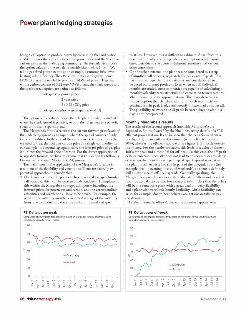
Monthly Margrabe’s resultsThe results of the second approach (monthly Margrabe’s) are depicted in figures 2 and 3 by the blue lines, using details of a 50% efficient power station. It can be seen that the peak forward curve (see figure 2) is currently in-the-money (with delta clearly above 50%), whereas the off-peak approach (see figure 3) is mostly out-of-the-money. For the nearby contracts, this leads to a delta of almost 100% for peak and almost 0% for off-peak. In this case, the off-peak delta calculation especially does not lead to an accurate nearby delta: even when the monthly average off-peak spark spread is negative, the plant is still expected to run in part of the off-peak hours (for example, during evening hours and weekends), so there is definitely still an exposure to off-peak spreads. Generally speaking, the Margrabe’s approach assumes a static dispatch pattern independent from the actual constraints. For example, this implies that the deltas will be the same for a plant with a great deal of hourly flexibility and a plant with very little hourly flexibility. Little flexibility can arise, for example, due to heat delivery obligations or take-or-pay constraints.

Further out on the off-peak curve, the opposite happens: over

0

20

40

60

80

100

120

Jan

11

Apr

11

Jul 1

1

Oct

11

Jan

12

Apr

12

Jul 1

2

Oct

12

Jan

13

Apr

13

Jul 1

3

Oct

13

Jan

14

Apr

14

Jul 1

4

Oct

14

Margrabe

Actual

%

F2. Delta power peakComparisonofpowerplantdeltasensitivitybasedonMargrabe’sformulaandMonteCarlosimulationapproachSource: KYOS

0

10

20

30

40

50

60

Jan

11

Apr

11

Jul 1

1

Oct

11

Jan

12

Apr

12

Jul 1

2

Oct

12

Jan

13

Apr

13

Jul 1

3

Oct

13

Jan

14

Apr

14

Jul 1

4

Oct

14

Margrabe

Actual

%

F3. Delta power off-peakComparisonofpowerplantdeltasensitivitybasedonMargrabe’sformulaandMonteCarlosimulationapproachSource: KYOS

November 2011 risk.net/energy-risk 67

Power plant hedging strategies

longer horizons, the off-peak spark spread is assumed to have a quite wide distribution, so can easily become positive. This leads to deltas going towards the 50%-mark. It is a general problem with the Margrabe’s formula that it assumes that the price dynamics can be described fully by daily returns and return correlations. In brief: it does not incorporate the concept of cointegration (Engel and Granger, 1987). Various researchers have shown the relevance of cointegration in today’s energy markets (Los, de Jong, van Dijken, 2009).

Delta sensitivity: full-simulation approach The limitations and biases of Margrabe’s formula as described above imply a more detailed calculation is required. The bias in the Margrabe’s formula when applied to power stations is too large to be ignored.

We believe a good solution does exist in the form of a more detailed calculation that looks at the optimal dispatch for a large number of scenarios, not only for the intrinsic scenario. Each scenario derives from a Monte Carlo simulation model of forward and spot prices, incorporating cointegration and other realistic market dynamics. Every dispatch schedule fulfils the actual physical constraints of the power station. For this we apply a plant dispatch model, based on a combination of dynamic programming and other optimisation techniques. The methodology of this dynamic programming model is excellently described in a paper (Tseng and Barz, 2002)

With this approach, a full Monte Carlo-based plant valuation on a typical power station may require as little as 30 seconds for one year and 200 scenarios. This is much faster than mixed-integer linear programming (MILP) dispatch software can achieve. Deltas can be derived by either: (a) shocking the prices per traded product and recalculating the plant value; or (b) taking the average production per traded product period.

It is our experience that the second approach, which can be performed in a second, gives very accurate results. The more accurate deltas are depicted in figures 2 and 3 by the red line. They are much more stable along the curve. There are two major explanations for this. First, the quite sharp hourly shaping of power spot prices makes the expected production pattern relatively similar now and in the future. Second, cointegration between power and fuel prices keeps spark spreads in a relatively narrow bandwidth.

The discussion so far has assumed that the relevant fuel prices are market quotes. In countries where a liquid spot market does not exist, plant owners are typically forced to use oil-indexed contracts to price natural gas. This is for example the case in the German market. As gas markets develop, an interim period may arise where plants use a combination of market fuel and oil-indexed contracts. Due to take-or-pay obligations, the relevant market price for dispatching can either be gas, oil or other commodities.

This creates an exposure to a variety of oil, coal and potentially foreign exchange prices.

Another advantage of the simulation approach is that this additional exposure can be derived as well. The individual exposures show up, as long as the dispatching routine incorporates the optimal switching between market gas and oil-indexed gas.

Conclusion In a dynamic environment, prices of all commodities vary continuously. This leads to continuous changes in spark and dark spreads, creating a need to hedge. The starting point of almost any hedging strategy is the calculation of the delta sensitivities. We have discussed two potential methods for calculation: the Margrabe’s formula and the Monte Carlo simulation approach. When comparing the two, Margabe’s deltas are often quite inaccurate. One explanation is that Margrabe’s does not incorporate the real hourly structure in price patterns, nor does it take into account the hourly dispatch constraints. Another explanation is that the Margrabe’s formula assumes that the price dynamics can be described fully by daily return volatilities and correlations, and ignores, for example, cointegration and spiky spot returns. Risk reporting, value attribution and hedge performance will improve via a full Monte Carlo simulation approach. Although this will take somewhat more time to calculate than Margrabe’s, we believe the benefits justify this effort. ■

Cyriel de Jong, Hans van Dijken and Alexandra Bundalova are consultants at Kyos Energy Consulting

References

Engle R and C Granger, 1987Co-integration and error correction: Representation, estimation and testingEconometrica 55(2), pages 251–276

Los HS, C de Jong and H van Dijken, 2009Realistic power plant valuationsWorld Power, pages 48–53

Tseng CL and G Barz, 2002Short-term generation asset valuation: a real options approachOperations Research, 50(2), pages 297–310

The Margrabe’s formula requires the current forward price levels of the underlying spread as an input, where the spread consists of only two commodities. In the case of the carbon markets, this means that we need to treat the fuel plus carbon price as a single commodity