46
Keras with Tensorflow back-end in R and Python Longhow Lam
| Date post: | 24-Jan-2018 |
| Category: |
Data & Analytics |
| Upload: | longhow-lam |
| View: | 2,368 times |
| Download: | 1 times |

Keras with Tensorflowback-end in R and Python
Longhow Lam
Agenda
• Introduction to neural networks &Deep learning
• Keras some examples• Train from scratch
• Use pretrained models
• Fine tune
Introduction to neural networks
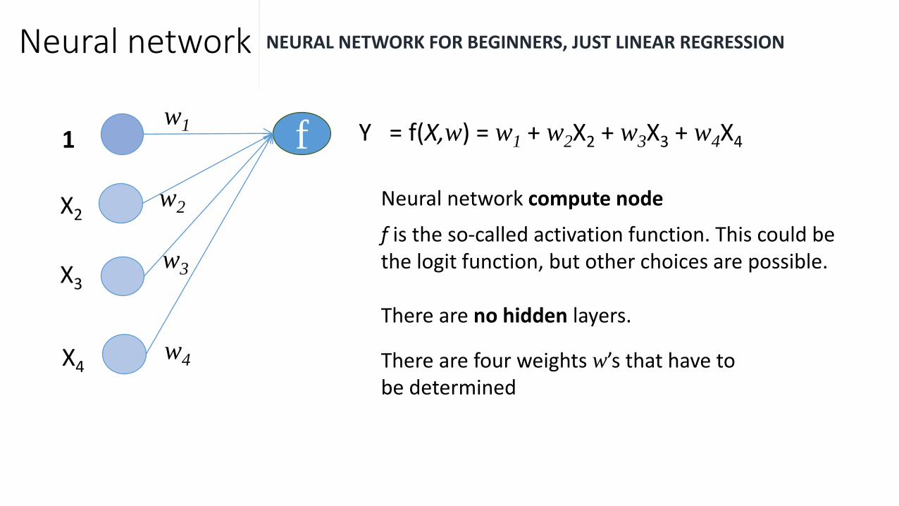
Neural network NEURAL NETWORK FOR BEGINNERS, JUST LINEAR REGRESSION
f Y = f(X,w) = w1 + w2X2 + w3X3 + w4X41
X2
X3
X4w4
w3
w1
w2 Neural network compute node
f is the so-called activation function. This could be the logit function, but other choices are possible.
There are no hidden layers.
There are four weights w’s that have to be determined

Neural networks ONE HIDDEN LAYER, MATHEMATICAL FORMULATION
Age
Income
Region
Gender
X1
X2
X3
X4
Z1
Z2
Z3
f
X inputs Hidden layer z outputs
α1
β1
neural net prediction f = 𝑔 𝑇𝑌
𝑇𝑌 = 𝛽0𝑌 + 𝛽𝑌𝑇𝑍
𝑍𝑚 = 𝜎 𝛼0𝑚 + 𝛼𝑚𝑇 𝑋
The function σ is defined as:
𝜎(𝑥) =1
1+𝑒−𝑥
𝝈 is also called the activation function,
In case of regression the function g is the Identify function I
In case of a binary classifier, g is the softmax 𝑔 𝑇𝑌 =𝑒𝑇𝑌
𝑒𝑇𝑁+𝑒𝑇𝑌
The model weights w = (α , β) have to be estimated from the data
m = 1, ... ,M
number of nodes / neurons in the hidden layer
Neural networks
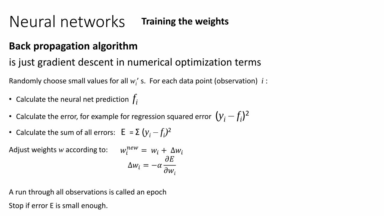
Back propagation algorithm
is just gradient descent in numerical optimization terms
Randomly choose small values for all wi’ s. For each data point (observation) i :
• Calculate the neural net prediction fi
• Calculate the error, for example for regression squared error (yi – fi)2
• Calculate the sum of all errors: E = Σ (yi – fi)2
Adjust weights w according to:
A run through all observations is called an epoch
Stop if error E is small enough.
Training the weights
𝑤𝑖𝑛𝑒𝑤 = 𝑤𝑖 + ∆𝑤𝑖
∆𝑤𝑖 = −𝛼𝜕𝐸
𝜕𝑤𝑖
Deep learning

Deep learning LOOSELY DEFINED:
NEURAL NET WORK WITH MORE THAN 2 HIDDEN LAYERS
Don’t use deep learning for ‘simple’ business analytics problems… it is really an overkill!
Keep it simple if you have ‘classical’ churn or response models: logistics regression, trees, or forests.
In this example all layers are fully connected (or also called dense layers)
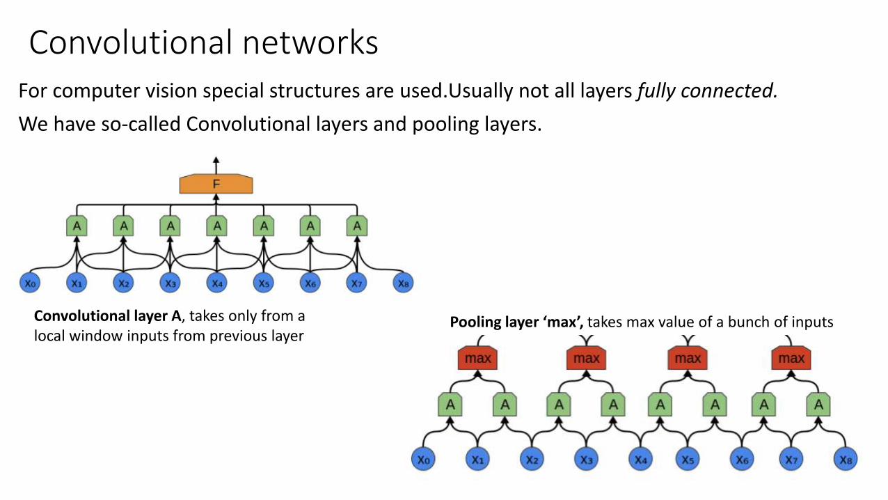
Convolutional networksFor computer vision special structures are used.Usually not all layers fully connected.
We have so-called Convolutional layers and pooling layers.
Convolutional layer A, takes only from a local window inputs from previous layer
Pooling layer ‘max’, takes max value of a bunch of inputs
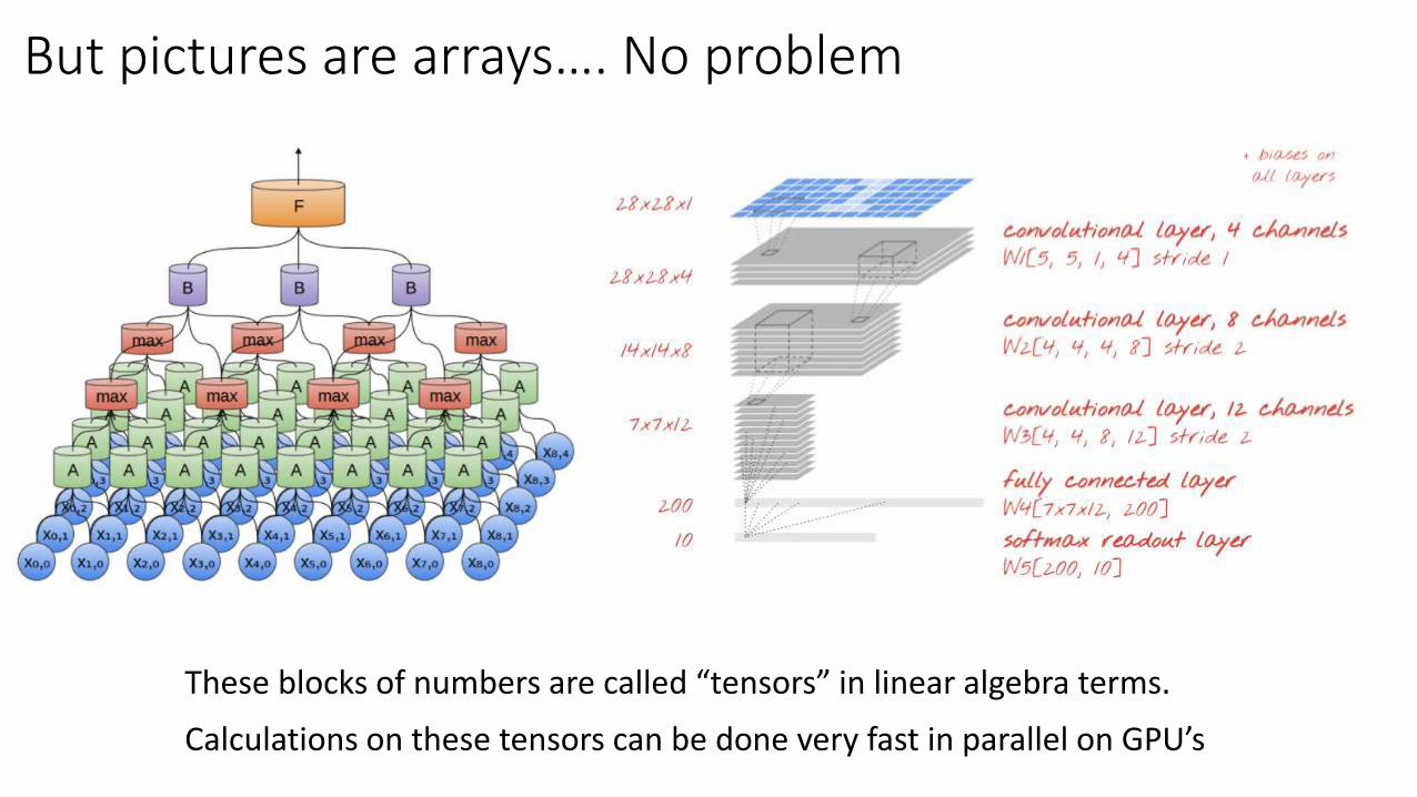
But pictures are arrays…. No problem
These blocks of numbers are called “tensors” in linear algebra terms.
Calculations on these tensors can be done very fast in parallel on GPU’s
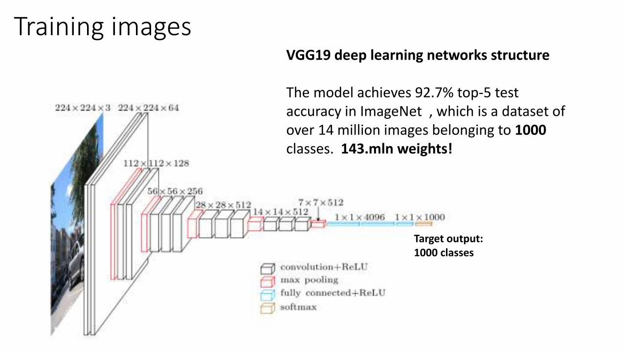
Training imagesVGG19 deep learning networks structure
The model achieves 92.7% top-5 test accuracy in ImageNet , which is a dataset of over 14 million images belonging to 1000classes. 143.mln weights!
Target output: 1000 classes

KERAS on Tensorflow
Keras
• Keras is a high-level neural networks API, written in Python and capable of running on top of either TensorFlow or Theano.
• It was developed with a focus on enabling fast experimentation.
• Being able to go from idea to result with the least possible delay is key to doing good research.
• Specifying models in keras is at a higher level than tensorflow, but you still have lot’s of options
• There is now also an R interface (of course created by Rstudio… )
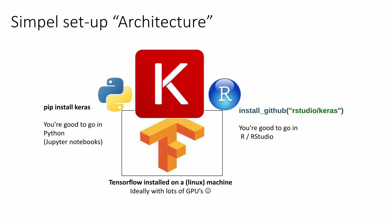
Simpel set-up “Architecture”
Tensorflow installed on a (linux) machineIdeally with lots of GPU’s
pip install keras
You’re good to go in Python (Jupyter notebooks)
install_github("rstudio/keras")
You’re good to go inR / RStudio

Training from scratch: MNIST example
MNIST data:
70.000 handwritten digits with a label (“0”, “1”,…,”9”)
Each image has a resolution of 28*28 pixels, so a 28 by 28 matrix

First a simple neural network in R
Treat image as a vector. It has length 784 (28by28), the number of pixels. One hidden layer (fully connected)
Pixel 3
Pixel 2
Pixel 1
Pixel 783
Pixel 784
neuron 1
neuron 256
Label 0
Label 9
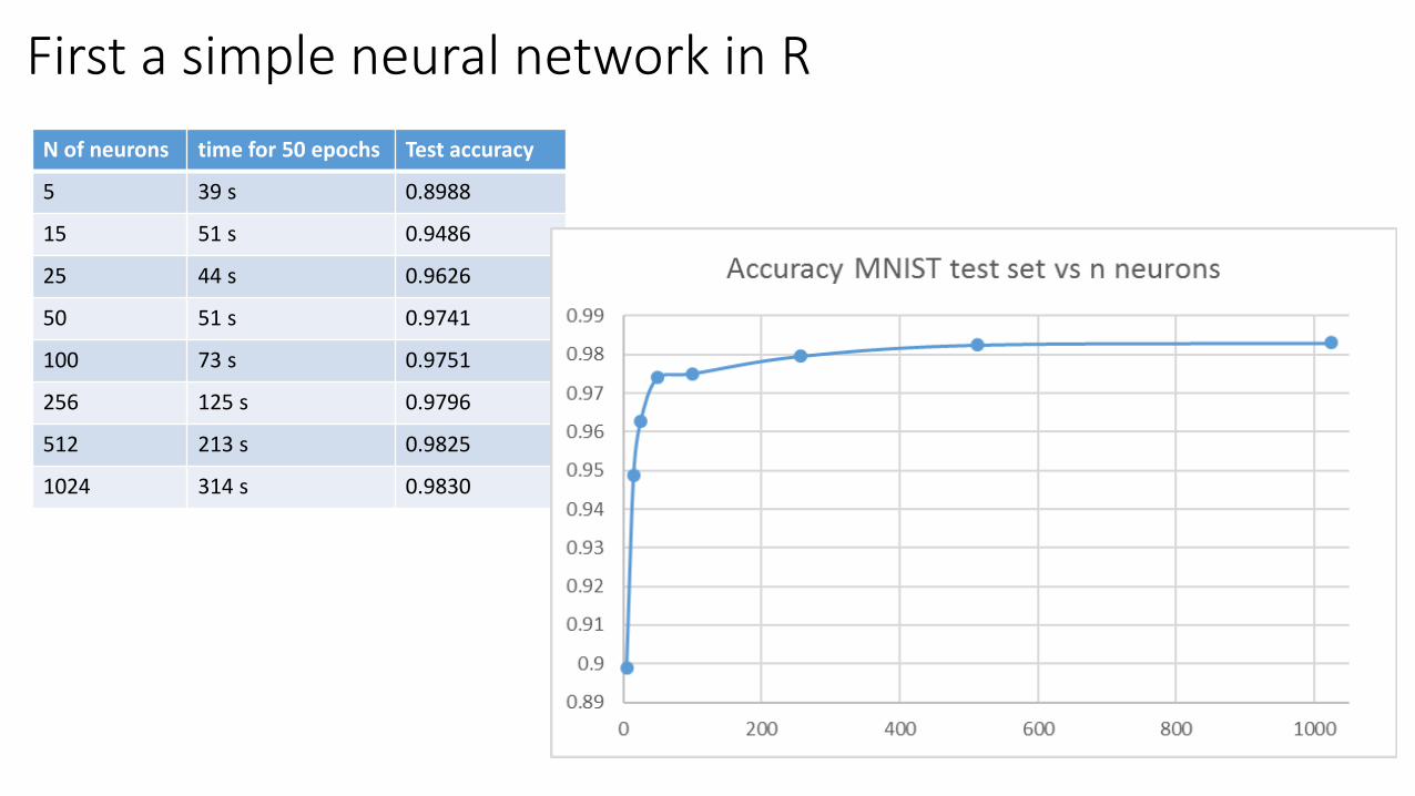
First a simple neural network in R
N of neurons time for 50 epochs Test accuracy
5 39 s 0.8988
15 51 s 0.9486
25 44 s 0.9626
50 51 s 0.9741
100 73 s 0.9751
256 125 s 0.9796
512 213 s 0.9825
1024 314 s 0.9830
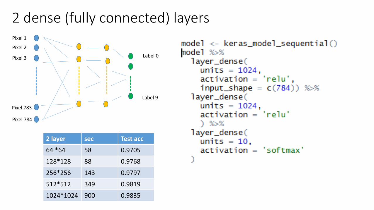
2 dense (fully connected) layers
2 layer sec Test acc
64 *64 58 0.9705
128*128 88 0.9768
256*256 143 0.9797
512*512 349 0.9819
1024*1024 900 0.9835
Pixel 3
Pixel 2
Pixel 1
Pixel 783
Pixel 784
Label 0
Label 9

A more complex model in Python
Images are treated as matrices / arrays• Convolutional layers• Pooling layer• Dropouts• Dense last layer
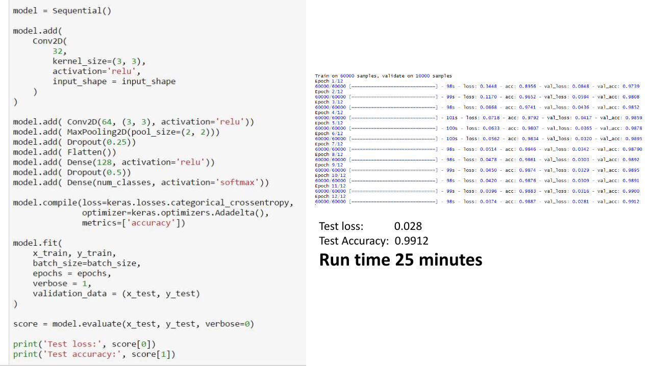
Test loss: 0.028Test Accuracy: 0.9912
Run time 25 minutes

Now compare with GPU
Some extra steps:
1. Spin up: Microsoft NC6 machine: 1 X Tesla K80 GPU ($1.084/hr)
2. Install CUDA toolkit / install cuDNN
3. pip install tensorflow-gpu
Run same model as in previous slide: Now it takes 2.9 minutes
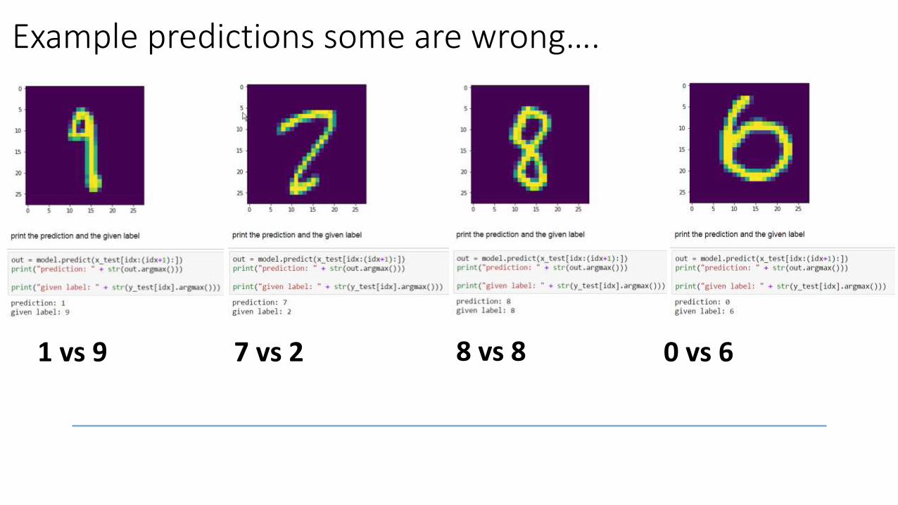
Example predictions some are wrong….
1 vs 9 7 vs 2 8 vs 8 0 vs 6
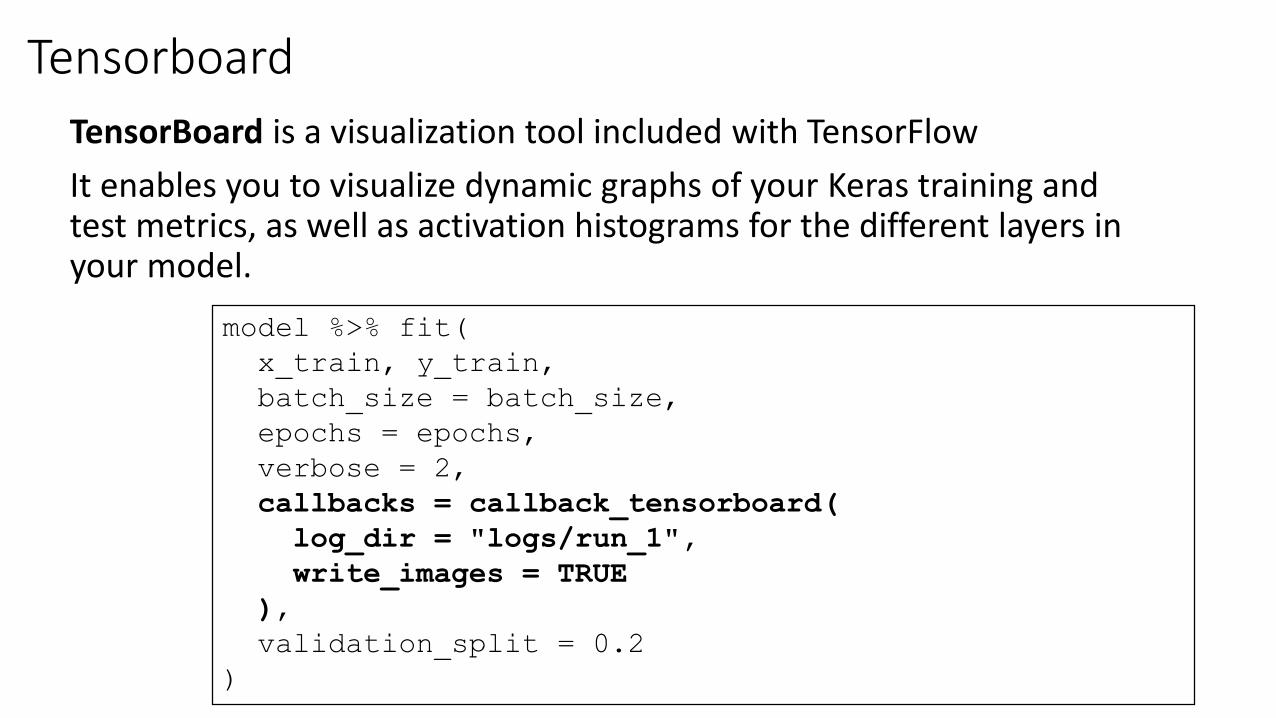
Tensorboard
TensorBoard is a visualization tool included with TensorFlow
It enables you to visualize dynamic graphs of your Keras training and test metrics, as well as activation histograms for the different layers in your model.
model %>% fit(
x_train, y_train,
batch_size = batch_size,
epochs = epochs,
verbose = 2,
callbacks = callback_tensorboard(
log_dir = "logs/run_1",
write_images = TRUE
),
validation_split = 0.2
)
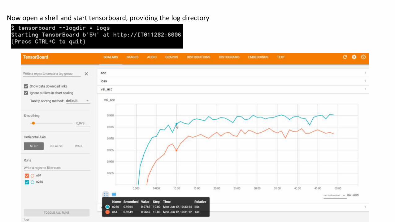
Now open a shell and start tensorboard, providing the log directory

Pre trained neural networks

Using pre-trained models
Image classifiers have been trained on big GPU machines for weeks with millions of pictures on very large networks
Not many people do that from scratch. Instead, one can use pre-trained networks and start from there.
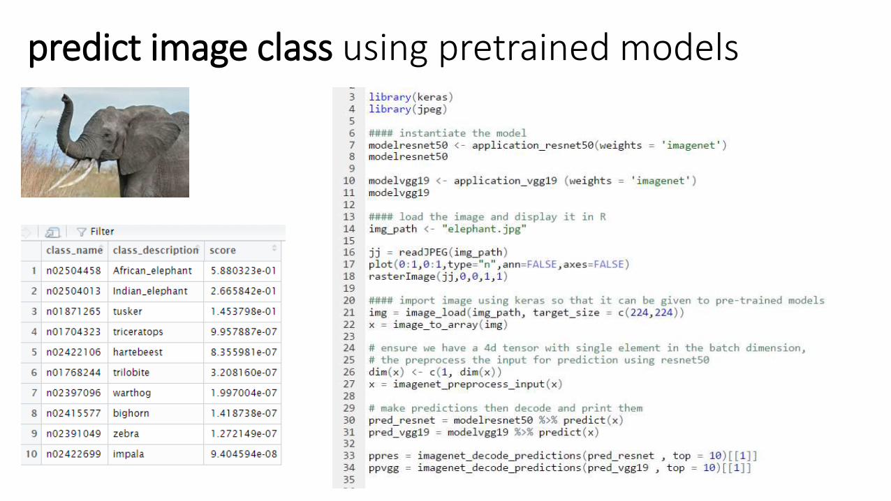
predict image class using pretrained models

RTL NIEUWS Images trough resnet and vgg16
Link to trellisJS app
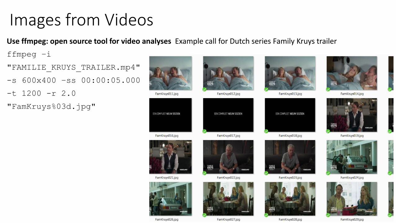
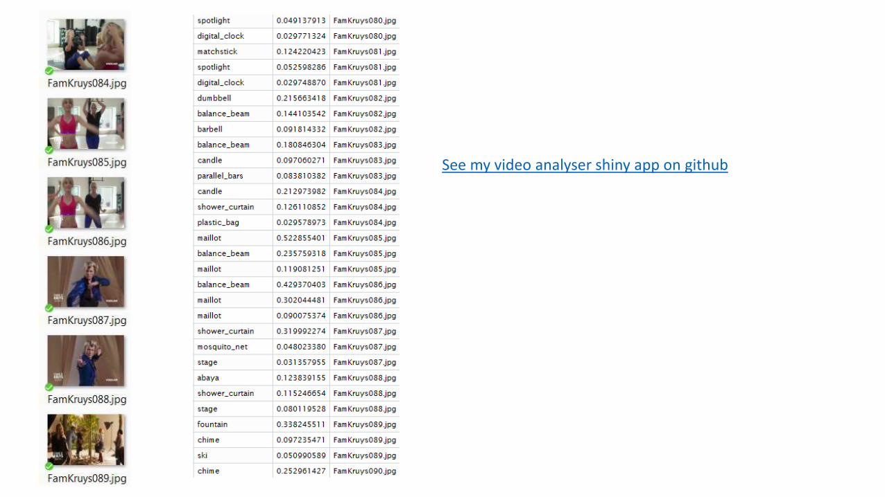
Images from VideosUse ffmpeg: open source tool for video analyses Example call for Dutch series Family Kruys trailer
ffmpeg –i
"FAMILIE_KRUYS_TRAILER.mp4"
-s 600x400 –ss 00:00:05.000
-t 1200 -r 2.0
"FamKruys%03d.jpg"
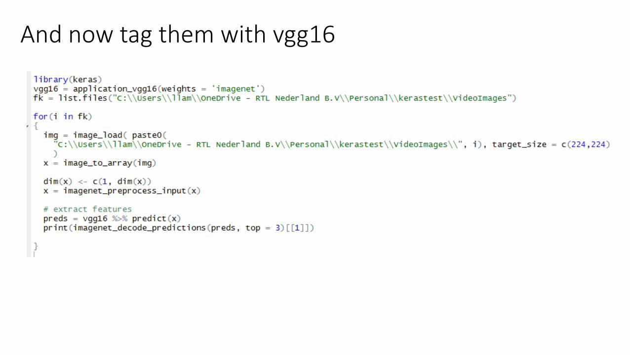
And now tag them with vgg16
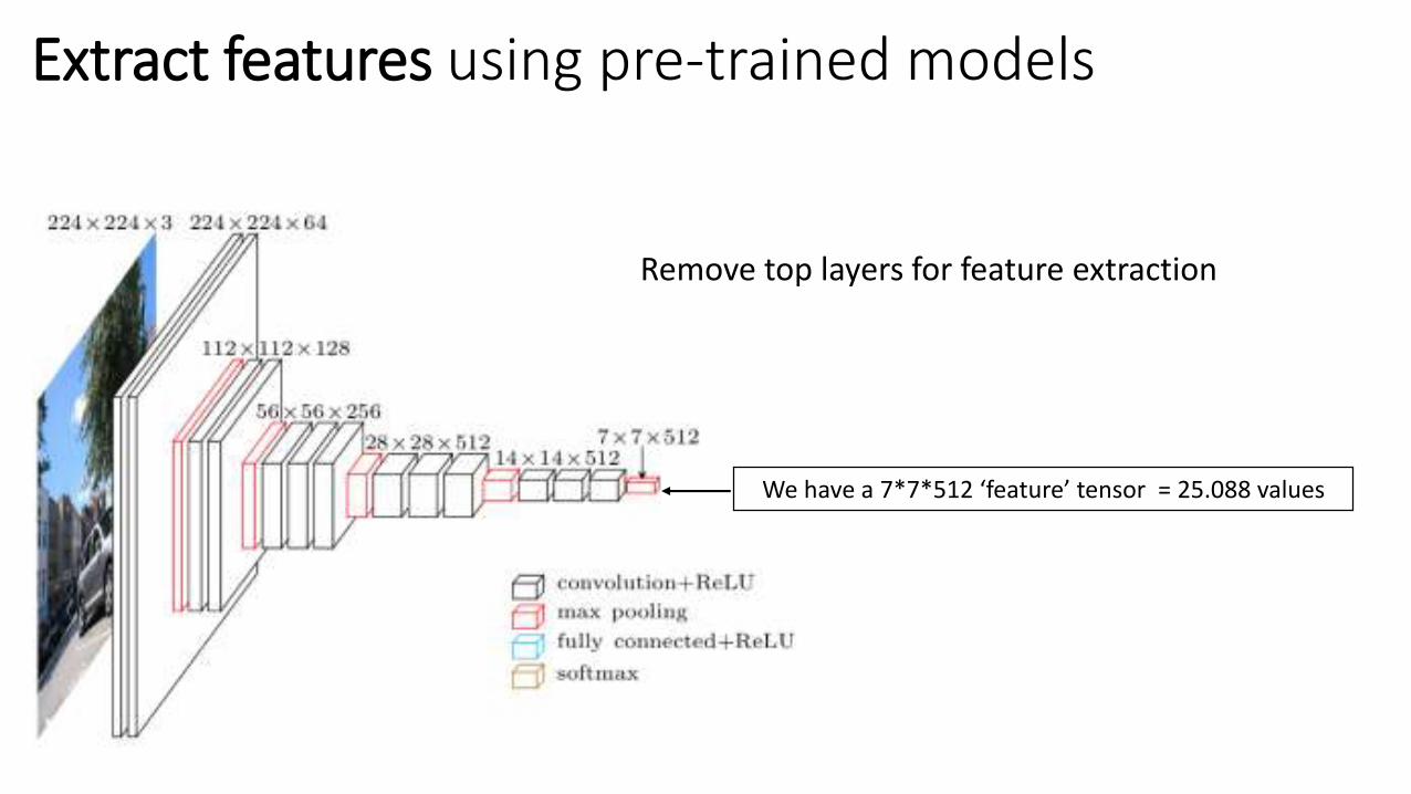
Extract features using pre-trained models
Remove top layers for feature extraction
We have a 7*7*512 ‘feature’ tensor = 25.088 values

Only a few lines of R code
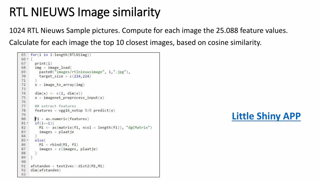
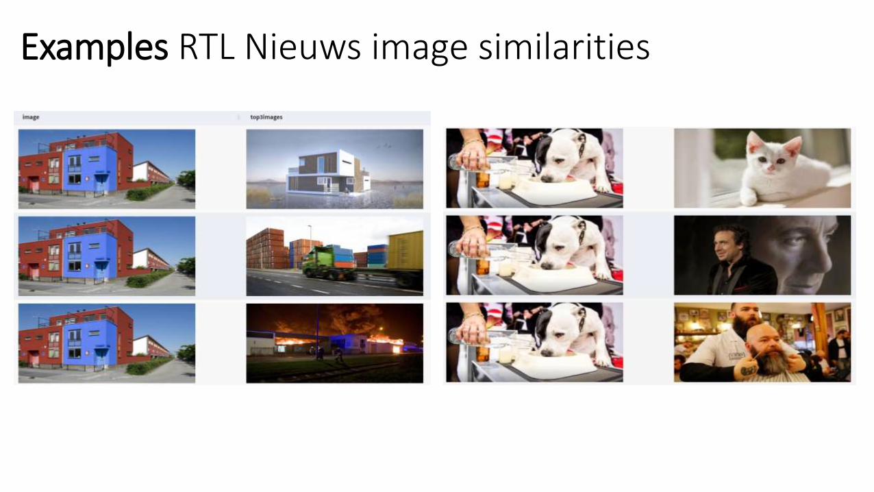
RTL NIEUWS Image similarity
1024 RTL Nieuws Sample pictures. Compute for each image the 25.088 feature values.
Calculate for each image the top 10 closest images, based on cosine similarity.
Little Shiny APP
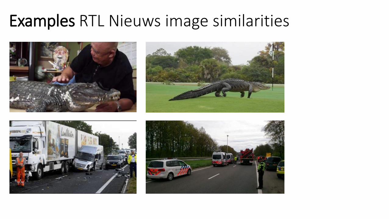
Examples RTL Nieuws image similarities
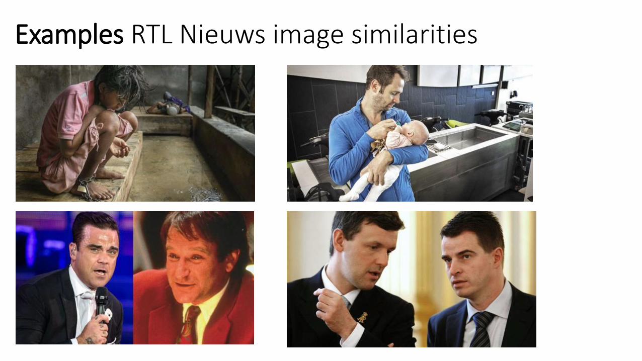
Examples RTL Nieuws image similarities
Examples RTL Nieuws image similarities

Same can be done for Videoland ‘boxarts’
See little shiny app

The Brad Pitt similarity index
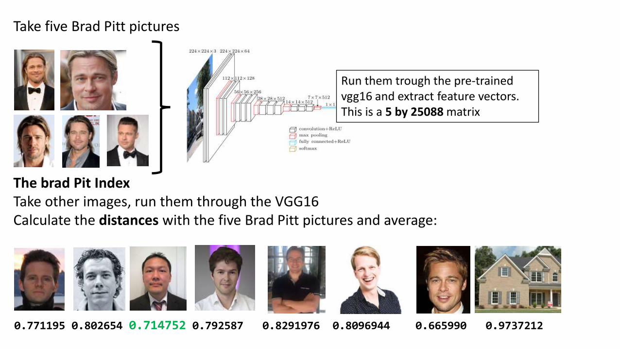
Take five Brad Pitt pictures
Run them trough the pre-trained vgg16 and extract feature vectors. This is a 5 by 25088 matrix
The brad Pit IndexTake other images, run them through the VGG16Calculate the distances with the five Brad Pitt pictures and average:
0.771195 0.802654 0.714752 0.792587 0.8291976 0.8096944 0.665990 0.9737212
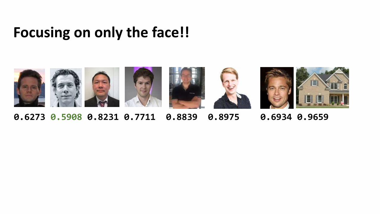
0.6273 0.5908 0.8231 0.7711 0.8839 0.8975 0.6934 0.9659
Focusing on only the face!!

Transfer learning / Fine tune pre trained models
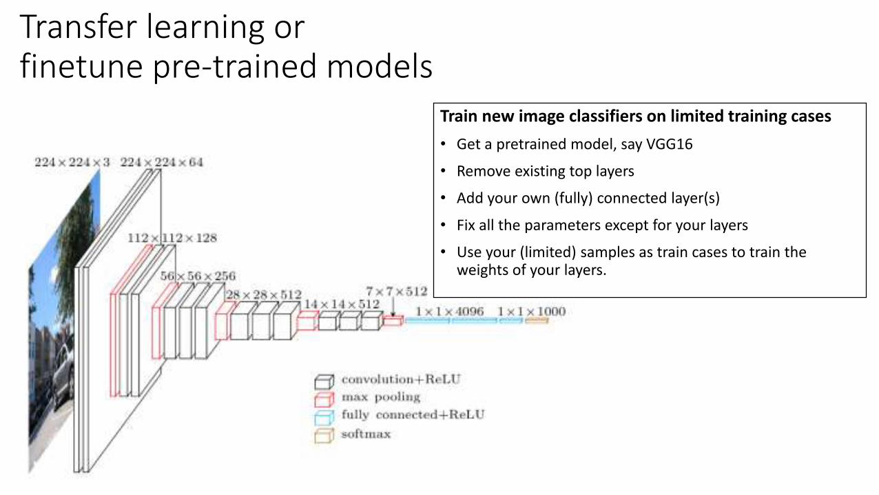
Transfer learning orfinetune pre-trained models
Train new image classifiers on limited training cases
• Get a pretrained model, say VGG16
• Remove existing top layers
• Add your own (fully) connected layer(s)
• Fix all the parameters except for your layers
• Use your (limited) samples as train cases to train the weights of your layers.

Python code examplebase_model = VGG16(weights='imagenet', include_top=False)
x = base_model.outputx = GlobalAveragePooling2D()(x)# let's add a fully-connected layerx = Dense(256, activation='relu')(x)
# and a logistic layer -- 2 classes dogs and catspredictions = Dense(2, activation='softmax')(x)
# this is the model we will trainmodel = Model(inputs=base_model.input, outputs=predictions)
# first: train only the top layers (which were randomly initialized)# i.e. freeze all convolutional layersfor layer in base_model.layers:
layer.trainable = False
# compile the model (should be done *after* setting layers to non-trainable)model.compile(optimizer='rmsprop', loss='categorical_crossentropy', metrics =['accuracy'])
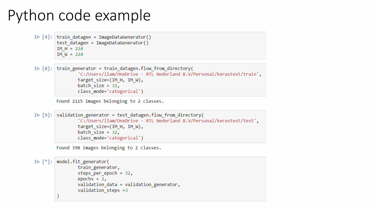
Python code example

1000 cats and dogs example