Key Factors Affecting 3D Reservoir Interpretation and ... · purpose workflows with a closed loop...

____________________________________________________________________________________________

*Corresponding author: E-mail: [email protected], [email protected];

British Journal of Applied Science & Technology3(3): 376-405, 2013

SCIENCEDOMAIN internationalwww.sciencedomain.org

Key Factors Affecting 3D ReservoirInterpretation and Modelling Outcomes:

Industry Perspectives

V. Singh1*, I. Yemez1 and J. Sotomayor1

1Repsol, Mendez Alvaro 44, Campus Azul (IIIrd Floor), 28045 Madrid, Spain.

Authors’ contributions

This work was carried out in collaboration between all authors. All authors read andapproved the final manuscript.

Received 19th January 2013Accepted 1st March 2013

Published 17th March 2013

ABSTRACT

To properly characterizing and modelling a hydrocarbon bearing reservoir is not an easytask because the reservoir properties vary spatially due to reservoir heterogeneities whichoccur at all scales, from pore scale to major reservoir units. The level of reservoircomplexities under study determines the quantity and quality of data requirements for 3Dreservoir modelling activity. An adequate understanding of the limitations imposed by thedata, associated uncertainty, or the underlying geostatistical algorithms or approaches andtheir input requirements for the 3D reservoir models are absolutely necessary to obtainreasonable production forecasts. Generally, industry look-backs continue to show thedifficulty of achieving a production forecast within an uncertainty band (P90 and P10) forboth “Greenfield” projects with limited data and “Brownfield” projects with abundant data.Some of the identified key factors affecting production forecasts are: sparse and non-representative data, biased estimates of Original Hydrocarbon In-Place, non-representative inputs distribution in the reservoir models, inadequate static and dynamicmodels, poor use of seismic data, use of improper analogs, non-unique history matchingcalibration processes for brownfields and inappropriate use of uncertainty workflows andtools. This paper briefly discusses some of these factors which affect 3D reservoirinterpretation and modelling outcomes for the conventional reservoirs, to provide betterunderstanding, propose effective and practical solutions to improve production forecastsbased on lessons learned from 3D reservoir modelling studies, authors and industryexperiences. In recent years, the industry has developed and used some high-level fit-for-

Review Article

British Journal of Applied Science & Technology, 3(3): 376-405, 2013

377

purpose workflows with a closed loop between 3D static and dynamic reservoir modellingunder uncertainty with use of appropriate geo-statistical techniques and history look-backsapproach which assist capturing the uncertainties in production forecasts and improvingthe project risks assessment. The evolution of closed loop modelling process will continueas new techniques and technologies are developed and implemented, enhancing ourability to capture the physical realities of the real subsurface world, generate betterproduction forecasts to reduce the risk associated with field developments.

Keywords: Reservoir characterization; modelling, facies; petrophysical parameters;simulation; production forecasts; uncertainty; risks.

ACRONYMS AND ABBREVIATIONS

2D/3D SEM – 2D-3D Scanning Electron Microscopy; 3D – Three Dimension; API –American Petroleum Institute; ASHM – Assist or Semi Automatic History matching; Bbls –Barrels; CPU – Central Processing Unit; E&P – Exploration and Production; EOR –Enhanced Oil Recovery; FIB –Focused Ion Beam; GOR – Gas Oil Ratio; HM – HistoryMatching; LPM – Lithotype Proportion Matirx; m – meter; MBO – Millions Barrels of Oil;Micro-CT – MicroComputed Tomography; MPS – Multiple Points Simulation; N/G – Net toGross Ratio; OHIP – Original-Hydrocarbon-In-Place; OOIP – Original-Oil-In-Place; OTC –Offshore Technical Conference; OWC - Oil Water Contact; P90, P50 and P10 – 90%, 50%and 10% probabilities; Pc – Capillary Pressure; PGS – Pluri-Gaussian Simulation; PVT –Pressure Volume Temperature; QA-QC – Quality Assurance Quality Control; SGS –Sequential Gaussian Simulation; SIS – Sequential Indicator Simulation; TI – TrainingImages; TSGS – Truncated Sequential Gaussian Simulation; TVDSS – true Vertical DepthSub Sea; Vp - Compressional (P) Wave Velocity; Vs – Shear (S) Wave Velocity; X-Ray CT –X-Ray Computed Tomography.

1. INTRODUCTION

Finding and developing oil and gas assets has always been a risky business. The industryhas a history of technological advances that have helped to reduce the risk, even asreservoirs and the way they are produced have grown in complexity. However, risk has notbeen fully reduced due to inherent uncertainties in the workflows used to generateproduction forecasts of the oil and gas fields [1-4]. According to Rose [5], in the last 20 yearsof the 20th century, E&P companies delivered only about half of the predicted reserves.Merrow [6] reported in his study that since 2003, the rate of success for E&P megaprojects(1 Billion US$) has declined from 50% to 22%. The main reason for industryunderperformance is attributed to use of evaluation methods that do not account for the “fulluncertainty”. More importantly, a disappointing 64% of these projects experienced seriousand enduring production attainment problems in the first 2 years after first oil or gas.

3D reservoir models are constructed for various purposes in the E&P business and supportvalue-based decisions including: (1) development planning, estimation of reserves,commerciality decisions, acquisitions or farm-in opportunities, re-development of old fieldsand (2) asset management throughout the production period, execution and monitoring,water flood / EOR planning, production cessation/ abandonment. The reservoir modellingprocess is cyclic and never really ends (new data, new technology or new analogs). Industry


378

experience clearly shows that production forecasts obtained from these 3D reservoir modelsare often highly uncertain for “Greenfield” as well as “Brownfield” projects [7,8].

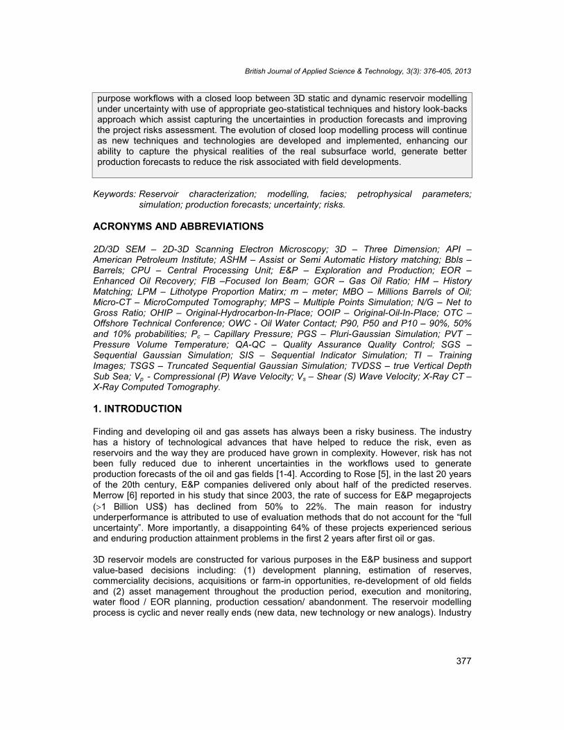
There are highly visible efforts in the industry to improve development planning andproduction forecast accuracy which are mainly driven by the E&P business needs,exponential growth in advances of computing since the early 90’s and advances in software(Fig. 1a). Today, existing computers can easily deliver teraflops (1012) to petaflops (1015).Improved parallel networking algorithms have significantly decreased the Central ProcessingUnit (CPU) run time by building large computers of distributed memory of up to 500 CPUmachines [9]. These rapid developments of CPU and technologies in computing advanceshave lead to:

The mathematical transformation of 10’s to100’s of terabytes of seismic datarecorded in a modern 3D seismic survey into high resolution subsurface images thatgeoscientists can interpret with higher confidence [10, 11].

Convert 3D seismic data into rock properties (Lithology, VP, VS, density, porosity,permeability, saturation, etc.) realizations through full wavefield and generalinversion which require intense computing resources [12, 13].

An exponential increase in cell counts since the 1990’s (from few thousands cells in1990’s to billions of cells in 2012) in 3D reservoir models (Fig. 1b). This isassociated with a significant decrease in the 3D reservoir model cell size from 300 -600m in 1990’s to 5 - 10m in 2012 as can be seen in Fig. 1c [14]. These 3Dreservoir models have allowed better capture of geological heterogeneities.

The reduced CPU run time for dynamic simulation which has significantly reduced oreliminated up-scaling of large size 3D static reservoir models (Fig. 1d). Highernumerical solution accuracy and flexibility to handle fully integrated Giga-Cell 3Dreservoir models, in-turn, has improved production forecasts predictability underuncertainty [15-17].

However, there are still several major issues in 3D reservoir modelling that need to beaddressed.

Some of these issues, related to the conventional clastic/carbonate reservoirs withoutfractures, are discussed along with effective and practical solutions proposed based onlessons learned from 3D reservoir modelling studies, authors’ and industry experiences. Thepresence of fractures in different reservoirs further adds the level of complexities on theseissues which are not considered in this paper. It is emphasized that if data QC, geologicalrules, mapping principles and geostatistics are not handled properly, the resulting model willbe less appropriate, regardless of the sophistication of the software and algorithmsdeployed. Therefore, in-depth understanding and incorporation of these aspects and use ofsubject experts’ knowledge from different disciplines in the 3D integrated reservoir modellingprocess is critical and will continue to improve reservoir modelling outcomes as new state-of-the-art techniques and technologies are developed and implemented. This in turn willenhance our ability to capture the physical realities of the real subsurface reservoirs andreduce the risk associated with field developments.


379

Fig. 1. (a)Increase in computation since 1993 based on top 500 computers (b) Increasein cell counts over the period 1991-2012) (Modified after Dogru, 2011) (c) Variation of

geological model size (decrease in cell size over the period 1991-2012) and (d)Reduction in computing time for a giga-cell model (Source: Dogru, 2011)

2. FACTORS CONTRIBUTING TO PRODUCTION FORECAST UNCERTAINTY

How can one interpret reservoir behaviours and trust production forecast capabilities of a 3Dreservoir model to be used for critical investment and decisions? To properly answer thisquestion, one must characterize and quantify all of the main uncertainties e.g. raw datameasurements, processing and interpretation, structure, stratigraphy, facies andpetrophysical modelling, transmissibility calculations and flow simulation inherent in the 3Dstatic and dynamic models. Techniques are used by calibrating models to availablemeasurement data and by propagating model inputs uncertainties to model outputs withhighest expected accuracy. Interpolating the models prediction is meant to improve theconfidence of a given simulation that has some predictive capability. The predictability andconfidence of these models are validated using some of the wells not used in the modellingor with of new wells drilled to prove the modelling outcomes. Some of the identified possiblecauses for production forecast uncertainty are:


380

Lack of tools that properly integrate all the data. Improper use of 3D reservoirmodelling and uncertainty workflows. Geostatistics failed to provide a solution formodelling many complex reservoirs and is very limited on the use of multiple seismicattributes. Modelling porosity with impedance as a soft constraint does not work inmany complex geologic settings because porosity is controlled by many otherfactors some of which are not represented by the impedance. Poor porosity modelsaffect the OHIP, 3D static and dynamic models. Usually, there is an incompleteevaluation of reservoir uncertainties and their impact on production forecasts is notfully analyzed.

Original or remaining Hydrocarbon In-Place generally too high due to:

Sparse data. Non-representative data: Biased to better reservoir quality. Inadequate or improperly analogs use.

Geological (static) models are inadequate due to:

Data limitation, quantity and quality. Failure to adequately model uncertainty. Optimistic N/G ratio distribution (reservoir versus non-reservoir). Inconsistent facies and reservoir properties distribution. Unidentified permeability contrasts-baffles/barriers, thief zones (reservoir

complexities not captured).

Simulation (dynamic) models are inadequate due to:

Data limitation, quantity and quality. Poor link between static and dynamic models. Poor and simplified up-scaling from fine to coarse grid used for history

matching & production forecasts (grid size). This is particularly critical whensecondary and tertiary recovery mechanisms (e.g. water flooding and gasinjection) are implemented.

Simplistic History matching procedures.

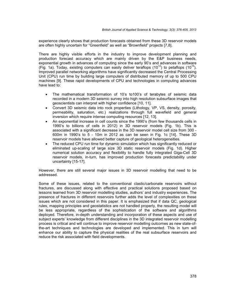
As part of the Quality Assurance-Quality Control (QA-QC) process within our company toimprove the technical quality of the portfolio of projects and reduce investment risk, a total ofaround fifty QA-QC events were carried out over a 5 years period. Around 47% of thefindings (recommendations for improvement) were related to 3D static and dynamic reservoirmodelling improvement opportunities (Fig. 2). These identified issues during the QA-QCprocess in different projects were very similar to those identified by the industry globally [7].


381

Fig. 2. Findings from QA-QC events in 3D reservoir modeling

2.1 Issues Related to Integrated 3D Reservoir Modelling Workflows

An efficient data management system for the vast amount of input data and softwareintegration is a critical component of the 3D reservoir modelling process. In a typical highlevel reservoir modelling and forecasting workflow (fast-track) used in the industry, the staticand dynamic models are built, honouring the limited available well data and may be a singleseismic attribute in the best case scenario, with no consideration of uncertainty. In thisprocess, typically, geological insights and seismic data are first interpreted and the resultsare combined with petrophysical interpretation and used to construct a static model. Duringthis process, most often, geostatistical techniques are misused due to lack of their goodunderstanding, proper application and lack of time to generate multiple realizations. As aresult, a single static model is then exported into the dynamic domain where a singleforecast is generated without any feedback between static and dynamic models. The datainterpretation involved in this process requires multiple assumptions to be made and thefeedback loops used to verify them are often very limited or non-existent. Anothershortcoming of the typical workflow is little or no focus on delivering uncertainty at each stepof the process related to dynamic outcomes. Typically, each discipline tries to pass adeterministic answer to the next one. Uncertainty is usually investigated at each step toexplore volumetric ranges and obtain history matches without any integrated QC of theadjusted ranges. This sequential modelling often makes it difficult to investigate the impact ofstatic model uncertainty in the dynamic realm, because the static parameters variability andits impact have effectively been predetermined. Interdependencies cannot be properlyidentified and history matches often lead to manipulation of dynamic parameters or arbitrarymodifications of permeabilities, without consistent changes to the precursor properties (suchas porosity, facies, saturation) from which they were derived.

To address these limitations of conventional modelling workflows, in recent years, theindustry has started using a closed loop modelling workflow in which the impact of allmodelling parameters and their uncertainties on a particular decision outcome are beingrepresented, i.e., the so called “high level closed-loop modelling and forecasting workflow”keeping in view the input data, modelling objectives and project timelines. In this workflow,


382

all the model components are simultaneously tested against an outcome, thereby quantifyingthe potential impact on uncertainty on development decisions. There are several papers andtext books that discuss the uncertainty assessment using different methodologies: (1)experimental design [18-24]; (2) Monte Carlo simulation [1,25] and; (3) stochastic approach[26-28].

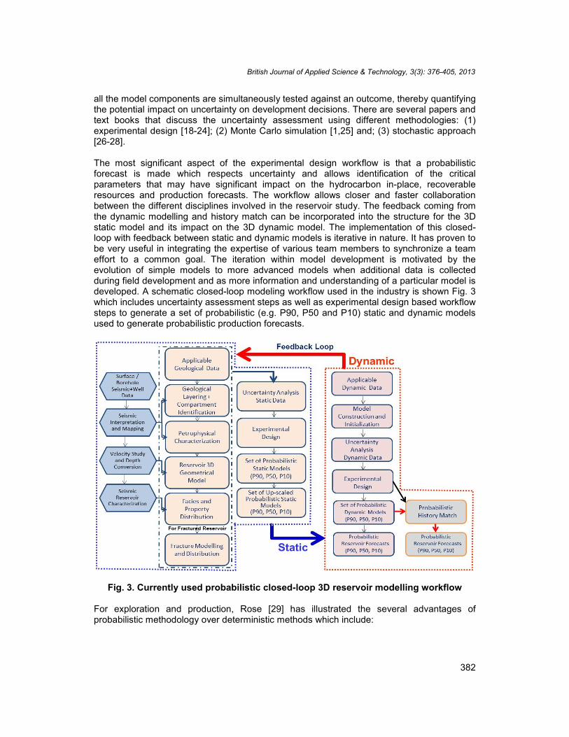
The most significant aspect of the experimental design workflow is that a probabilisticforecast is made which respects uncertainty and allows identification of the criticalparameters that may have significant impact on the hydrocarbon in-place, recoverableresources and production forecasts. The workflow allows closer and faster collaborationbetween the different disciplines involved in the reservoir study. The feedback coming fromthe dynamic modelling and history match can be incorporated into the structure for the 3Dstatic model and its impact on the 3D dynamic model. The implementation of this closed-loop with feedback between static and dynamic models is iterative in nature. It has proven tobe very useful in integrating the expertise of various team members to synchronize a teameffort to a common goal. The iteration within model development is motivated by theevolution of simple models to more advanced models when additional data is collectedduring field development and as more information and understanding of a particular model isdeveloped. A schematic closed-loop modeling workflow used in the industry is shown Fig. 3which includes uncertainty assessment steps as well as experimental design based workflowsteps to generate a set of probabilistic (e.g. P90, P50 and P10) static and dynamic modelsused to generate probabilistic production forecasts.

Fig. 3. Currently used probabilistic closed-loop 3D reservoir modelling workflow

For exploration and production, Rose [29] has illustrated the several advantages ofprobabilistic methodology over deterministic methods which include:


383

Accuracy of estimates can be measured, so estimator can be accountable. Use of statistical tools improves the estimates. Predrill reality checks can detect errors before drilling. Reserves/resources estimation is faster, more efficient and avoids false precision. Realistic communication of uncertainty to decision makers and investors is

facilitated. Results are immediately usable in modern portfolio measurement.

However, there are several shortcomings in the normally used tools (e.g. stochastic,probabilistic, Monte Carlo simulation results) for uncertainty and impact assessments. Someof the important quotes for these statistical tools by the industry experts [30] are as follows:

“The crucial weakness of the stochastic approach is in the inability to assignprobabilities with any degree of certainty”.

“Monte Carlo simulation results are only as good as the subjective inputassumptions of the user”.

“Assigning probabilities to the decision tree branches requires technical expertise aswell as considerable domain knowledge, and specialists from many disciplines haveto be called in for subjective judgement about critical parameters”.

“Apparent capture of uncertainty through probability distributions encouragesintellectual laziness”.

“Simulation lacks the ability to incorporate a wide range of knowledge - key todecision making - from analog fields and studies”.

“Real reservoirs are so complex that the available elegant mathematical tools usedto quantify uncertainty and risks are only of limited use”.

In many ways these shortcomings are still valid. Therefore, understanding the basicassumptions, input requirements for the specific statistical technique used in the 3Dreservoir modelling process, use of expert knowledge from different disciplines with theirskills, selection of appropriate workflows and quality checking of the data as well as theresults at every step of the process are critical to achieve the defined objectives of 3Dreservoir modelling.

2.2 Impact of Limited Data (Quantity and Quality) on Ohip Estimation inGreenfields (Appraisal and Early Development Phases)

Often during exploration and appraisal stages of different projects, relatively safe wells aredrilled with the focus to obtain data that will confirm the presence of significant amount of oiland gas. The data obtained from these wells is used along with analog data/information tosupport the technical evaluation (OHIP, recoverable resources/reserves, well productivity,production forecasts, etc.) and further E&P activities. Authors experience on different E&Pprojects continue to show the difficulty of achieving hydrocarbon-in-place estimates withinthe evaluated uncertainty band (P90 and P10). This is usually due to the uncertainties ofdifferent input parameters and their ranges which are often not estimated properly. This ismainly due to two problems: (1) Need of more data to be acquired as the project moves fromone stage to the next during the early asset life and (2) suboptimal or limited use of existingdata/information.

There are very limited examples available in public domain database (Journals/conferences)where history look-backs shows the evolution of different input parameters range (gross rock


384

volume, porosity, N/G ratio, permeability, saturation, fluid contacts, etc.) and hydrocarbon-in-place estimates over time and the impact of additional data on reduction of uncertainties[31]. When available, they demonstrate that the hydrocarbon-in-place uncertainty look-backapproach has been highly useful in tracking the impact of new data.

There is a need for comprehensive assessment of uncertainties upfront and developing anunderstanding of their impact from the existing data/ information and how these uncertaintiesevolve with time as new data/ information is acquired. The importance of new data has beendemonstrated in this section and the optimal use of existing data/information with differenttechniques and appropriate workflows have been elaborated in the next sections.

The example shown here is from a carbonate field in which a total of 6 wells have beendrilled so far including the discovery well which demonstrates the value of newdata/information. The field is a 4-way dip closure (interpreted based on 3D seismic data)bounded by the east and west side normal faults. The reservoir depth at different welllocations is in the range of 4300-4500m TVDSS. Currently, this field is producing around30,000 Bbls/day oil from 5 producers.

The predrill mean resources for this prospect were around 190 MBO. The discovery well-Aencountered a gross reservoir thickness of around 128m, a net pay of 72m and a well-defined oil water contact. The well test confirmed a daily production of around 5000 Bbls/dayof 30 API oil with GOR of 700scf/Bbl. Second well-B drilled, close to the eastern fault,encountered a gross reservoir thickness of around 242m, a net pay of 190m and lower OWCas compared to Well-A but indicated more reservoir heterogeneity than assumed afterdiscovery. Well-C drilled in the centre part of the structure between two wells and it went dry.Well-D drilled towards to the west of Well-B encountered oil bearing reservoir but with adifferent OWC. Well-E drilled in the western part of the structure up-dip to well-Aencountered oil with similar OWC as found in well-A. Well-F drilled towards the north part ofconfirmed the OWC of Well-B.

The primary pore system in this carbonate reservoir comprises inter-particle porosity thatcoexists with a highly variable secondary system of dissolution voids. As a consequence, thereservoir heterogeneity (from pore to reservoir scale) and its variability pose significantchallenges to data acquisition, petrophysical evaluation, and reservoir description. Theconventional petrophysical evaluations that exclusively use reservoir zonation based on thelithology/mineralogy have very limited application. For identifying the distribution of micro-porosity and its connectivity with macro-porosity, advanced down-hole technologies such ashigh-resolution imaging, magnetic resonance logs with advanced core analysis have provento be very useful.

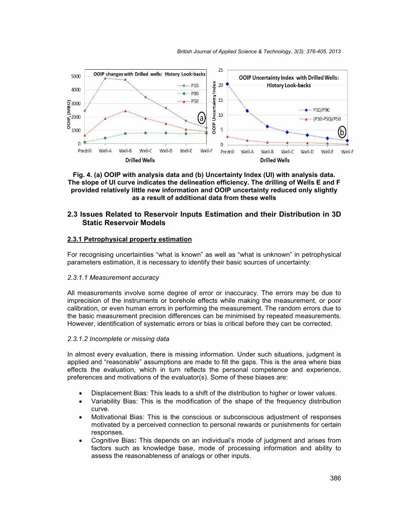
The reservoir and fluid parameters were estimated after the drilling of each well integratingpreviously available data (Table 1). The Original-Oil-In-Place (OOIP) for different categories(P90/P50/P10) was estimated using probabilistic approach. The OOIP uncertainty index and2P recoverable resources were computed after each well following similar workflow ofevaluation. Fig. 4 shows the summary of hydrocarbon-in-place and uncertainty changes overthe appraisal and early development period. The history look-backs approach used hereclearly demonstrates the effective value addition from each drilled well and the evolution ofOOIP, recoverable resources including reduction in OOIP uncertainty.


385

Table 1. Summary of reservoir and fluid parameters estimated after each drilled well

Key parameters Predrill Well-A Well-B Well-C Well-D Well-E Well-FReservoir Top (m) 4350 4404 4363 4456 4414 4394 4497Gross Interval (m) 80 128 242 24 120 138 189Net Pay (m) 56 72 190 0.0 81.5 76 87N/G 0.70 0.56 0.78 0.00 0.68 0.55 0.46Porosity (av.) 10% 9.5% 12.9% 6% 12% 10% 13%Water Saturation 36% 18.3% 27% 39% 36% 22% 25%Formation Volume Factor 1.38 1.37 1.25 1.25 1.25 1.25 1.25Oil Water Contact (m) ------- 4532 4572 None 4505 4532 4572Cut-offs (Vcl/Phi/Sw) 0.5/0.05/0.5 0.5/0.05/0.6 0.5/0.05/0.6 0.5/0.05/0.6 0.5/0.05/0.6 0.5/0.05/0.6Oil API Gravity 25-30 30 30 30 30 30GOR (SCF/Bbl) 500 750 670 ----- 700 740 740CO2/H2S Content (%) 2-5% / none 2-5% / none 2-5% / none 2-5% / none 2-5% / none 2-5% / none 2-5% / noneGas Gravity 0.90- 1.06 0.90- 1.06 0.90- 1.06 0.90- 1.06 0.90- 1.06 0.90- 1.06 0.90- 1.06Reservoir Pressure (psi) 6800-7648 7225 7310 ----- 7268 7242 7344OOIP (P90/P50/P10)(Millions BO)

120/635/2450 425/1874/4850 765/2450/4750 810/1890/3458 800/1503/2650 756/1070/1700 789/926/1185

RF 30% 30% 25% 18% 18% 18% 18%P50 RR(Millions BO) 190 562 613 340 270 193 167Uncertainty Index 1(P10/P90)

20.42 11.41 6.21 4.27 3.31 2.25 1.50

Uncertainty Index 2(P10-P50)/P50

2.86 1.59 0.94 0.83 0.76 0.59 0.28


386

Fig. 4. (a) OOIP with analysis data and (b) Uncertainty Index (UI) with analysis data.The slope of UI curve indicates the delineation efficiency. The drilling of Wells E and Fprovided relatively little new information and OOIP uncertainty reduced only slightly

as a result of additional data from these wells

2.3 Issues Related to Reservoir Inputs Estimation and their Distribution in 3DStatic Reservoir Models

2.3.1 Petrophysical property estimation

For recognising uncertainties “what is known” as well as “what is unknown” in petrophysicalparameters estimation, it is necessary to identify their basic sources of uncertainty:

2.3.1.1 Measurement accuracy

All measurements involve some degree of error or inaccuracy. The errors may be due toimprecision of the instruments or borehole effects while making the measurement, or poorcalibration, or even human errors in performing the measurement. The random errors due tothe basic measurement precision differences can be minimised by repeated measurements.However, identification of systematic errors or bias is critical before they can be corrected.

2.3.1.2 Incomplete or missing data

In almost every evaluation, there is missing information. Under such situations, judgment isapplied and “reasonable” assumptions are made to fill the gaps. This is the area where biaseffects the evaluation, which in turn reflects the personal competence and experience,preferences and motivations of the evaluator(s). Some of these biases are:

Displacement Bias: This leads to a shift of the distribution to higher or lower values. Variability Bias: This is the modification of the shape of the frequency distribution

curve. Motivational Bias: This is the conscious or subconscious adjustment of responses

motivated by a perceived connection to personal rewards or punishments for certainresponses.

Cognitive Bias: This depends on an individual’s mode of judgment and arises fromfactors such as knowledge base, mode of processing information and ability toassess the reasonableness of analogs or other inputs.


387

2.3.1.3 Computational approximations

Approximations inherent in the workflows and methodologies used for estimatingpetrophysical properties such as Vcl, effective porosity, permeability, saturation, cut-offs, andin defining the electrofacies/facies based on petrophysical properties.

To illustrate these aspects, four separate studies were performed for estimating the effectiveporosity in a carbonate reservoir using same log data, core data and software followingsimilar approach shown by Meddaugh et al. [7]. These are: Study A: focused on overallmatch between core and log data for full field, Study B: Best overall match by well, Study C:Best match in higher porosity zones and Study D: Artificial intelligence methods usingmultiple logs for all the wells.

A crossplot of effective porosity values is generated between study C and other studies toshow the variances (Fig. 5) for this reservoir. Porosity of around 14% will be known typicallyonly within an error of 2 units. The solid line shows the 1:1 line and the dashed lines show± 2 porosity units relative to the 1:1 line. Each approach could be technically acceptable butthe variation does bring into focus the potentially large uncertainty associated with what istypically regarded as a “known” in reservoir uncertainty assessments.

Fig. 5. Porosity comparison between three studies A, B, C and D using same data andsoftware

The lessons drawn from this example are valid for other petrophysical properties (e.g.saturation, permeability, net reservoir and fluid contacts), although not discussed here.Therefore, it is recommended to determine uncertainties for the critical petrophysicalparameters including raw data, its processing and interpretation. Most often, the largestuncertainty in petrophysical evaluation may be the interpretation model itself. The knowledgeof possible ranges of petrophysical properties will improve the 3D reservoir modellingresults; enabling better data gathering and study decisions.

2.3.2 Facies identification and rock typing

Most often, simple sand / carbonate shale models are generated without facies analysis.Core data is one of the critical inputs for facies classification. In absence of core,electrofacies can be used as a basis for facies identification. Well log data provide veryuseful information on geological concepts, stratigraphic details and petrophysical properties.


388

Most often, capillary pressure (Pc) curves are used in dynamic modelling as input fordefining oil-in-place and vertical distribution of fluids in a reservoir. These Pc curves canhave significant influence on fluids movement within a model, if not designed adequately.For a displacement process that is controlled by gravity, Pc curves control vertical saturationdistribution. These Pc curves also allow definition of the top of the transition zone and itsthickness which affects to control water/gas breakthroughs time and trends. Often it hasbeen observed that these Pc curves have failed to match initial water saturation at welllocations if they are not analyzed and incorporated based on proper facies / rock typingusing core and log data (Figs. 6a, b and c) in the 3D reservoir models. The impact of usingsingle rather than several rock types for water saturation can be clearly seen in Fig. 6d. Inorder to ensure proper fluids in place volume estimation from simulation modelsinitializations, it is necessary to obtain an acceptable level and trend of matching betweenwater saturation log profiles with simulation models profile for each interval within thereservoir to reduce the gap between static and dynamic models. Integration of the capillarypressure, water saturation and resistivity index results, together with the basic petrophysicaldata including porosity, permeability, NMR, CT scans, mercury injection and thin sectionimages confirm the validity and consistency of the collected data and allows a more robustevaluation of the facies and rock typing.

Fig. 6. (a) Electrofacies typing based on log data, (b) Rock typing based on Core data,(c) Rock typing based on Log data and (d) Comparison of capillary pressure curves

derived versus log derived initial water saturation

2.3.3 Reservoir facies and property distributions

The rock and fluid properties control the volume of Original-Hydrocarbon-In-Place (OHIP)and the recoverable oil gas. Different techniques are used for populating the reservoir faciesand properties in the 3D reservoir models besides geostatistics which require different typesof input parameters and work under different basic assumptions. Therefore, the simulationresults obtained from these techniques are highly dependent on a geomodeler’s


389

geostatistical knowledge and geological experience. For better understanding we groupthem in two categories:

Variogram based techniques. Variogram-free techniques.

2.3.3.1 Variogram based techniques

The variogram models play an extremely important role in representing the geologicalknowledge in 3D static reservoir model building and in analyzing flow behaviours throughdynamic simulation. Variogram, a statistical device to store patterns in a mathematical form,is a “measure of geological variability with distance” (reservoir geometry, continuity andproperties) and is developed using two point statistic correlation functions [32,33]. Almost90% of the reservoir characterization studies use variogram based geostatistical modellingmethods (e.g. Sequential Gaussian Simulation (SGS), Sequential Indicator Simulation (SIS),Truncated Sequential Gaussian Simulation (TSGS), Pluri-Gaussian Simulation (PGS), etc.).These algorithms (SGS, SIS, TSGS, PGS) create a 3D model constrained to local data andthe variogram model [34-36].

The SGS technique distributes reservoir properties (facies, porosity and permeability) within3D model while honouring data at the wells and corresponding vertical and lateral correlationlengths using variograms. This technique does not constrain reservoir properties usingexplicit geological facies information. The variogram cannot be calculated directly from rawdata of reservoir properties because SGS needs inputs to be in a normal distribution.Variograms are calculated using normal score variables. The normal score variables arelater transformed back to reproduce their original distribution. Experimental variograms arecalculated from the well data for normal score variables for the reservoir properties in verticaland lateral directions. This technique is most commonly used for facies distribution but doesnot guarantee honouring of boundary conditions and requires variograms.

The SIS technique for continuous variables divides the continuous distribution of a particularvariable into a number of discrete categories. Each category represents a specific rangewithin the continuous distribution of the attribute. The categories are distributed within thefine scale grid cell using SIS. Similar to SGS, the SIS technique does not constrain reservoirproperties using explicit geological facies information. However, SIS groups similar propertyvalues together. SIS requires an indicator variogram for each category of property which arecalculated for vertical and lateral directions using well data for all indicators. This techniquelacks ability to honour facies boundary conditions and requires a user defined trend(variograms) to impose non-stationarity. SIS is most commonly used for petrophysicalproperties distribution.

The TSGS technique is used to generate the underlying geological framework of the facies.This facies framework together with SGS, is then used to distribute reservoir propertiesvalues separately within each facies. This technique honors the explicit geological faciesinformation at the wells, vertical and lateral correlation lengths for each facies, verticalstratigraphic facies trends, reservoir properties from well data, as well as vertical and lateralcorrelation length of reservoir properties for each facies. This technique allows integration ofboth geological and petrophysical data to generate reservoir description. It works well forgrain size transitions and ordered facies (e.g. carbonate environments, shoreface deposits,progradational fluvial sequences) and requires variograms as input. The TSGS technique,also known as transition modelling, allows for only strict facies boundary conditions and it


390

becomes very unstable in the presence of high density (closely spaced) wells. Non-stationarity further compounds the problem as introduction of simple trends is often notsufficient.

The Plurigaussian simulation is an extension of the truncated (mono) Gaussian method[37,38] allowing for more complex facies relationships under a strict stratigraphic sequence.The geological information is added to the model by: number of Gaussian functions,correlation coefficient among them, facies proportion to calculate thresholds, direct andcross indicators covariances, facies data at conditioning points transformed into Gaussianrules and truncation strategy (rock type rule). There are numerous advantages of PGS overother facies simulation methods. PGS handles non-stationarity through use of multiplevertical proportion curves in the construction of a lithotype proportion matrix (LPM). The LPMconsists of hundreds of high resolution trend maps accounting for vertical and lateral non-stationarity. The trends for each facies within each layer and every reservoir interval in themodel are calculated. This technique is capable of capturing most inter- and intra-faciesrelationships including post depositional overprinting, such as diagenesis. As a pixel basedmethod, PGS can work in the presence of closed spaced or sparse well control but is moresuitable for high density well controls. However, it is important to note that PGS results arehighly dependent on a geomodeler’s geostatistical knowledge and geological experience.

Depending upon the particular simulation algorithm, different types of variogram models(Nugget, Linear, Logarithmic, Gaussian, Spherical, Elliptical, Exponential, Power, etc.) areselected which require different data inputs for computing the variogram parameters (sill,nugget and range) to be used for facies and property distribution in 3D reservoir models.

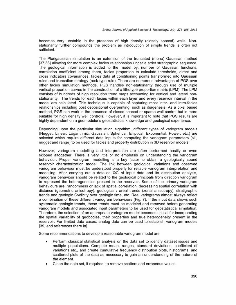
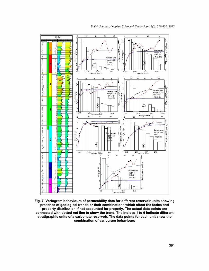
However, variogram modelling and interpretation are often performed hastily or evenskipped altogether. There is very little or no emphasis on understanding the variogrambehaviour. Proper variogram modelling is a key factor to obtain a geologically soundreservoir characterization model. The link between geological variations and observedvariogram behaviour must be understood properly for reliable variogram interpretation andmodelling. After carrying out a detailed QC of input data and its distribution analysis,variogram behaviour should be related to the geological principals from direction variogramto represent the heterogeneities present in the reservoir. Some of the primary variogrambehaviours are: randomness or lack of spatial correlation, decreasing spatial correlation withdistance (geometric anisotropy), geological / areal trends (zonal anisotropy), stratigraphictrends and geologic Cyclicity over geologic time, etc. Real variograms almost always reflecta combination of these different variogram behaviours (Fig. 7). If the input data shows suchsystematic geologic trends, these trends must be modeled and removed before generatingvariogram models and associated input parameters to be used for geostatistical simulation.Therefore, the selection of an appropriate variogram model becomes critical for incorporatingthe spatial variability of geobodies, their properties and true heterogeneity present in thereservoir. For limited data cases, analog data can be used to establish variogram models[39, and references there in].

Some recommendations to develop a reasonable variogram model are:

Perform classical statistical analysis on the data set to identify dataset issues andmultiple populations. Compute mean, ranges, standard deviations, coefficient ofvariations etc., and create cumulative frequency distribution plots, histograms, andscattered plots of the data as necessary to gain an understanding of the nature ofthe element.

Clean the data set, if required, to remove scatters and erroneous values.


391

Fig. 7. Variogram behaviours of permeability data for different reservoir units showingpresence of geological trends or their combinations which affect the facies andproperty distribution if not accounted for properly. The actual data points are

connected with dotted red line to show the trend. The indices 1 to 6 indicate differentstratigraphic units of a carbonate reservoir. The data points for each unit show the

combination of variogram behaviours


392

Analyse the spatial distribution of the data to determine the suitability forgeostatistical analysis. If the data is not suitable, then perform a statistical analysisusing interpolation techniques to prepare it as input for variogram modelling.

Analyse only one variable per lithologic unit at a time and ensure that this variable isstationary over the domain of the study. If the input data has mixed population split itinto subsets with unique population parameters because variogram analysis usingmixed populations can produce misleading results.

Check if the data has the same sample length i.e., sample of different size should beseparated as a different groups of variogram.

Visualise samples for irregular distributions to ensure approximately uniform sampledistribution for variography.

Transform data to standardized normal distribution (zero mean and unit variance). Itsimplifies the data handling and allows the comparison between different data sets.

Follow a three step process to combine qualitative geological knowledge withquantitative variogram modelling: (1) Generate detailed interpretation of geologicalaspects of the reservoir, including environment, sequence stratigraphy, pore spacecharacteristics, iso-chores, iso-porosity, and iso-permeability maps. Using theseinputs, generate a summary table that includes the major continuity direction, lateralextension and anisotropy index of each attribute, (2) Calculate experimentalvariogram using averaging technique and (3) Model the variogram considering theinformation summarised in the first step.

Generate omnidirectional / multidirectional experimental variograms and variogrammaps using the procedure mentioned in the previous point to identify the nugget, sill,anisotropy and major direction of the variogram analysis. Use relevant seismicattributes to compute areal variograms, if seismic data quality is acceptable and welldata to compute vertical variograms.

2.3.3.2 Variogram free techniques

Variogram based simulation techniques (e.g. SGS, SIS, TSGS, PGS) allow construction offacies and properties model conditioned to well, seismic and production data. However,simulated depositional elements do not look geologically realistic as two point statisticalcorrelation functions are not sufficient to model curvilinear or long range continuousgeological bodies. Some other techniques, which do not use variograms, are either objectbased or use other numerical techniques: Multiple Point Simulation [40]; SimulatedAnnealing [41,42,13]; Artificial Neural Networks [43,44,12]; Genetic Algorithms [45-47];Fuzzy Logic [48-50]. Some of them are briefly described below:

2.3.3.2.1 Multiple point simulation (MPS)

The MPS technique, a pixel as well as an object based algorithm, aims at characterisingpatterns using several points (does not require variogram models), typically between 20 and100, instead of two, thus providing more realistic representation of geological patterns. TheMPS technique requires various parameters for facies dimension and geometries (thickness,length, width, orientation, etc.) and is capable of handling many wells, seismic data, faciesproportion maps and curves, variable azimuth maps and interpreted geobodies. It works wellfor complex facies relationships but requires a large number of wells, training images (TI),outcrop mapping or any other source that produces a high resolution exhaustive model atthe same scale as the simulation to capture the spatial patterns for facies and properties [51-55]. The use of TI is not compulsory for the MPS technique; the statistics can come from


393

other sources. Nevertheless, a training image is the most convenient way of deriving the MPstatistics as most desired statistics can be extracted directly with no need to fit them withpositive definite models. The largest stumbling block that prevents the rapid spread of MPSin reservoir simulation tasks is the difficulty of creating TI’s for each definite modelling case.A TI is a 3D conceptual model or pattern that defines the basic laws of property alternationacross space and is a bridge between geological knowledge of the reservoir and thenumerical model. TI’s have the following requirements:

Three dimensional spaces. Stationary, i.e., invariability of the statistical parameters of the TI throughout its

volume. Although, now some modern MPS techniques also work with non-stationaryTI’s.

Recurrence, i.e. repeated use of the same structure elements; Aperiodicity, i.e., no part of the TI may be an identical copy of another part of this TI;

the structure elements must vary in different combinations to cover all the possiblevariants.

Relative simplicity, i.e., the TI must not abound in complex structures that may notbe reproduced in the realizations.

The scale and orientation of the TI measured in grid cells are to be set according tothe field being simulated.

Statistical parameters, such as mean, variograms, unit compartmentalization (pernumber of cells) and dimensions of geological bodies are matched against well dataand target values.

However, the implementation of the MPS technique is quite difficult. Several differentapproaches have been used in the industry: single and extended normal equations, neuralnetwork iterative approach, simulated annealing. As an example, the training images ofporosity obtained from integration of wells and seismic data using different techniques (e.g.krigging, multi-attribute transforms using linear regression, neural networks, combination ofgeostatistics and neural networks), will lead to different spatial distributions, uncertaintyranges and errors [12,44], if used in MPS. Therefore, each of these methodologies has theirown limitations which affect the simulation results. The MPS techniques are still an emergingarea of research and require further R&D efforts to supplement the currently used traditionaltwo-point statistics (e.g. krigging, stochastic simulations).

2.3.3.2.2 Seismic guided techniques (e.g. multi-attribute regression, principal componentattributes analysis, artificial neutral networks, simulated annealing, fuzzy logic,genetic algorithms)

Currently, the industry is also using some techniques separately which allow generatinglithology, porosity and permeability 3D cubes using post- and pre-stack seismic attributesderived from 3D seismic data. These 3D cubes are directly transformed into the 3D reservoirmodels grid and used as inputs for defining reservoir stratigraphy, populating the reservoirand nonreservoir facies along with their properties particularly away from the well locations.All these techniques use validation process through use of blind wells and newly drilledresults to prove their ability to predict reservoir properties at unknown locations butcomparison between them shows that level of errors and uncertainty ranges are entirelydifferent in each technique. Therefore, proper understanding of these techniques, theirassumptions and limitations are critical before using them to generate inputs for 3D reservoirmodelling. Most often it has been observed that seismic data quality does not allow


394

extracting meaningful seismic attributes which limits the use of these techniques. The detailsof these algorithms are beyond the scope of this paper.

It is important to note that each simulation algorithm (variogram based, non-variogram basedand others) has specific input requirements, work under own basic assumptions andboundary conditions, some advantages as well as disadvantages which need to be properlyunderstood. Under these circumstances “which one to use” or “use their combination”. Inpractice, a geomodeler often chooses one algorithm before another based on personalexperience or competences, software capability, or some technical requirements. It is oftendifficult to obtain inputs for these algorithms due to limited subsurface data. Faciesinterpreted from well logs and core data have very high vertical resolution but very poorlateral resolution. Choosing input parameters is often subjective and the problem becomesespecially severe in the lateral directions if seismic attributes are not meaningful. Severalpublished studies have shown that use of different techniques with the same input data (welland core) provide significantly different production forecasts [7,40,53,56-58]. Therefore, athorough understanding of the assumptions and boundary conditions for each simulationalgorithm is necessary before they are used in 3D reservoir modelling.

2.3.4 Permeability measurements and upscaling

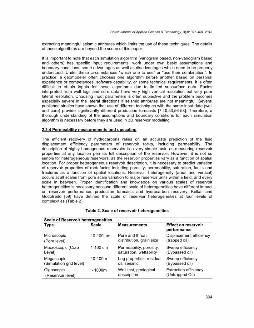
The efficient recovery of hydrocarbons relies on an accurate prediction of the fluiddisplacement efficiency parameters of reservoir rocks, including permeability. Thedescription of highly homogenous reservoirs is a very simple task, as measuring reservoirproperties at any location permits full description of the reservoir. However, it is not sosimple for heterogeneous reservoirs, as the reservoir properties vary as a function of spatiallocation. For proper heterogeneous reservoir description, it is necessary to predict variationof reservoir properties of rock facies including porosity, permeability, saturation, faults andfractures as a function of spatial locations. Reservoir heterogeneity (areal and vertical)occurs at all scales from pore scale variation to major reservoir units within a field, and everyscale in between. Proper identification and knowledge on various scales of reservoirheterogeneities is necessary because different scale of heterogeneities have different impacton reservoir performance, production forecasts and hydrocarbon recovery. Kelkar andGodofredo [59] have defined the scale of reservoir heterogeneities at four levels ofcomplexities (Table 2).

Table 2. Scale of reservoir heterogeneities

Scale of Reservoir heterogeneitiesType Scale Measurements Effect on reservoir

performanceMicroscopic(Pore level)

10-100 m Pore and throatdistribution, grain size

Displacement efficiency(trapped oil)

Macroscopic (CoreLevel)

1-100 cm Permeability, porosity,saturation, wettability

Sweep efficiency(Bypassed oil)

Megascopic(Simulation grid level)

10-100m Log properties, residualoil, seismic

Sweep efficiency(Bypassed oil)

Gigascopic(Reservoir level)

1000m Well test, geologicaldescription

Extraction efficiency(Untrapped Oil)


395

In 3D reservoir models, the permeability variation is represented on a block-centred gridusing a permeability value measured directly from core-plugs or estimated indirectly fromwireline log data using predictive algorithms that relate core data intergranular permeabilityto porosity including some other predicting variable. The key issue is how to use micorscopic(pore throat and grain size)) and macroscopic (core) measurements without introducingartifacts due to indiscriminate transgression of scale as the volume of a typical model gridblock ( 108 cm3) is several orders of magnitude greater than that sampled by a core-plugor wireline log (30-30,000 cm3). It is therefore necessary to upscale the permeability valuesfrom measurement scale to grid-block scale [60,61]. In order to fully understand the effect ofsample volume on the effective single phase permeability of a heterogeneous clasticreservoir, Jackson et al. [62] have carried-out direct measurements using a large rockspecimen (38x32x10 cm). They carried out measurements of permeability in different sizesof samples (starting from 1x1x1 cm to 38x32x10 cm) and observed that both individual andaveraged effective permeability values vary as a function of sample volume, which indicatesthat permeability data obtained from core-plugs will not be representative at the scale of areservoir model grid-block regardless of the number of measurements taken. At smallsample volumes, the distributions of horizontal and vertical permeability are very broad. Asthe sample volume increases, both the horizontal and vertical permeability distributionsnarrow and converge upon the effective permeability of the entire rock specimen. They alsonoted that the average permeability estimated from different samples do not correspond tothe effective permeability of the entire rock specimen.

To understand the permeability upscaling for highly heterogeneous carbonate reservoirs,which hosts around 50% of the world’s hydrocarbons, several laboratory measurements ofporosity and permeability between whole core samples and plugs drilled from the samesamples have been carried out. More recently, the heterogeneity of carbonates at the porescale using powerful image registration techniques (e.g. micro-CT, 2D SEM, 3D SEM/FIB, X-ray-CT, etc.) have been studied to characterize the fine scale structural framework ofcarbonates [61,63-65]. These studies indicate that permeability differences between wholecore and plugs vary greatly sample to sample but whole-core permeability tends to be higherin cases where large differences (two orders of magnitude) are observed.

Different averaging upscaling algorithms (Arithmetic mean, Harmonic mean, Geometricmean) used for permeability upscaling give different results but perform reasonably wellwhen applied to a field of permeability value covering full core-plug. The permeabilityupscaling becomes more critical where reservoir units have high property contrasts and isnot fully represented by the available standard core-plugs. However, the error introduced byaveraged data may be minimised using an appropriate averaging scheme for a given faciestype and flow direction. Conventionally, the arithmetic mean is used to average thepermeability measurements in the horizontal direction (parallel to the bedding), whilegeometric or harmonic mean is used to average permeability measurements in verticaldirection (perpendicular to the bedding). This approach is based on the assumptions thateach core-plug does sample only one lithology (or permeability class). In many geologicalsystems, core-plugs generally sample a mixture of lithologies (or permeability classes) andthe variations in lithology are not simply layered or uncorrelated. The most suitableaveraging technique in such cases is the one which minimises the variation in meanpermeability with sample volume rather than the one which yields the effective permeabilityof a layered or uncorrelated system. Well test data is one of the important inputs forcalibrating the upscaled permeability model as well test represents the large scalepermeability. However, the quality of well test data and its interpretation should always bekept in mind before using it for calibration as it is an effective permeability. The permeability


396

upscaling from pore to reservoir and field scales in different types of reservoirs is still achallenging task and require further R&D efforts to fully understand and establish thesuitable methodology.

2.4 Issues Related to 3D Dynamic Modelling

The objectives of dynamic reservoir modelling are to simulate the reservoir dynamicbehaviour, forecast reservoir parameters for undrilled locations and field productivity fordifferent development scenarios using 3D static reservoir model as an input. The simulationstudies directly integrate geological parameters with engineering data (e.g. production tests,pressure data) but this integration of data requires time and an understanding of reservoirmechanisms. A basic workflow of 3D dynamic modelling consists of 5 steps: (1) dataacquisition, (2) model design, (3) initialization, (4) history matching and (5) forecast. Mostoften, the 3D dynamic models are built separately without proper use of a 3D static model orusing 3D static model that rely-on only well data and ignore the lateral and verticalheterogeneities revealed in the key seismic attributes or with a poor link between static anddynamic models. The main inputs for the dynamic models can be classified as follows:

Petrophysical data:- Absolute/relative permeability, porosity, water saturation, N/Gratio, capillary pressure, rock types.

PVT Data:- Oil properties (density, formation volume factor, gas-oil solution ratio,viscosity and saturation pressure), gas properties (gas gravity, compressibility factor,formation volume factor, viscosity) and water properties (density, formation volumefactor, viscosity, compressibility).

Reservoir Data:- Depth of fluid contacts, initial pressure at a given depth,temperature and aquifer parameters.

Production Data:- Production / Injection fluid rates, bottom hole and tubing headflowing pressure measurements, static bottom hole pressure values.

Completion Data:- Well productivity and injectivity index, wellbore diameter skinfactor (i.e. permeability reduction near wellbore due to drilling and completion mudinvasion).

Well and / or field constraints:- Target (maximum) production / injection rate,maximum water rate, maximum gas-oil ratio, minimum flowing bottom hole andminimum tubing head pressure.

Economic Requirements:- Minimum oil and gas production rates, maximumproduction rate.

Dynamic simulation workflows for Greenfield and Brownfield projects are discussedseparately.

2.4.1 Greenfield 3D dynamic modelling

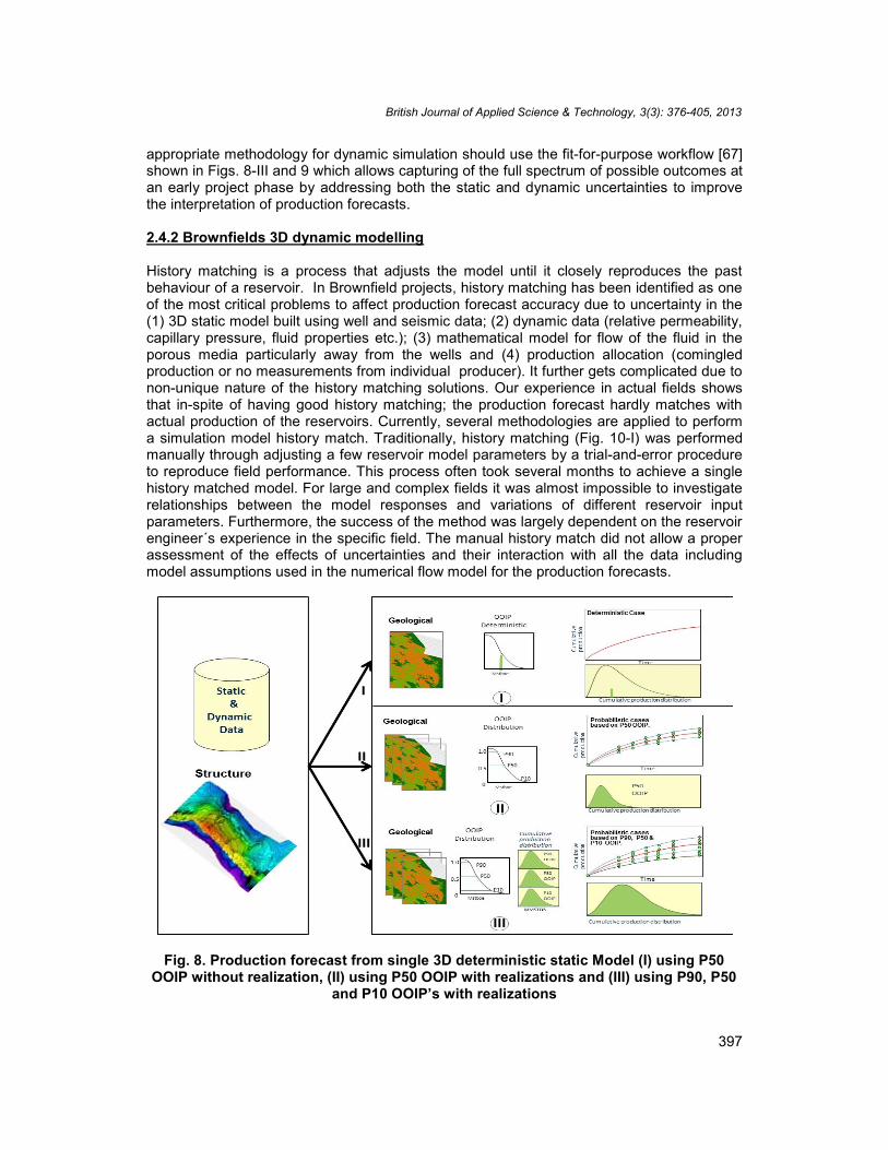
The uncertain production forecasts obtained from 3D dynamic simulation are particularlycritical for offshore “Green Fields” where capital intensive investment decisions are taken forthe field development. The risk of such decisions is that the whole development program, inmany cases, is decided based on deterministic or probabilistic models built with a verylimited amount of available data / information, inadequate workflows and the impact ofreservoir uncertainties on predicted production forecasts is not properly captured (Figs. 8-Iand 8-II). As a result, this leads to either over or under-sizing of the production facilities,impacting overall project value [66]. Depending upon the geological complexities, the


397

appropriate methodology for dynamic simulation should use the fit-for-purpose workflow [67]shown in Figs. 8-III and 9 which allows capturing of the full spectrum of possible outcomes atan early project phase by addressing both the static and dynamic uncertainties to improvethe interpretation of production forecasts.

2.4.2 Brownfields 3D dynamic modelling

History matching is a process that adjusts the model until it closely reproduces the pastbehaviour of a reservoir. In Brownfield projects, history matching has been identified as oneof the most critical problems to affect production forecast accuracy due to uncertainty in the(1) 3D static model built using well and seismic data; (2) dynamic data (relative permeability,capillary pressure, fluid properties etc.); (3) mathematical model for flow of the fluid in theporous media particularly away from the wells and (4) production allocation (comingledproduction or no measurements from individual producer). It further gets complicated due tonon-unique nature of the history matching solutions. Our experience in actual fields showsthat in-spite of having good history matching; the production forecast hardly matches withactual production of the reservoirs. Currently, several methodologies are applied to performa simulation model history match. Traditionally, history matching (Fig. 10-I) was performedmanually through adjusting a few reservoir model parameters by a trial-and-error procedureto reproduce field performance. This process often took several months to achieve a singlehistory matched model. For large and complex fields it was almost impossible to investigaterelationships between the model responses and variations of different reservoir inputparameters. Furthermore, the success of the method was largely dependent on the reservoirengineer´s experience in the specific field. The manual history match did not allow a properassessment of the effects of uncertainties and their interaction with all the data includingmodel assumptions used in the numerical flow model for the production forecasts.

Fig. 8. Production forecast from single 3D deterministic static Model (I) using P50OOIP without realization, (II) using P50 OOIP with realizations and (III) using P90, P50

and P10 OOIP’s with realizations


398

Fig. 9. Production forecasts for reservoirs having complex structure and geology.Different 3D static reservoir geological models are built and used as inputs for

dynamic simulation. Final cumulative distribution was generated by combining themand capturing the full uncertainties

Fig. 10. Production forecasts using (I) manually calibrated 3D static and dynamicmodels and (II) multiple calibrated 3D static and dynamic reservoir models capturing

full range of uncertainties

In order to improve the shortcoming of traditional history matching, the industry has shifted toother methods such as an Assisted or Semi-automatic History Match (ASHM) process [17] tofind multiple matched models, instead of a single set of model parameters that match thedata (Fig. 10-II). This helps to assess the production forecast uncertainty. ASHM is aprocess to compare historical and dynamic data by means of a misfit function [68]. It uses a


399

misfit function as objective function to bind the problem with the model constraints and cangenerate multiple calibrated models. The major problem with ASHM is the lack of robustnessand it requires different algorithms for different kinds of reservoir models. It is almostimpossible to use a unique algorithm or workflow to provide an accurate match of anyreservoir. ASHM technology will require some more time to become a mature technologywhich is more users friendly and flexible (to generate more reliable production forecasts inless time). Most of the existing algorithms have only proved to be very efficient with specificsynthetic cases. But the majorities have failed or were only partially successful with realcomplex reservoirs.

Although, the history match process helps to understand the interactions betweenheterogeneity and fluid flow and gives better reliability to the static and dynamic model, agood history match does not guarantee a more accurate production forecast. Some of therecommended best practices for a good history match are:

Know data quality, quantity and its limitations. Establish dynamic simulation objectives clearly and demonstrate how history match

variables correspond to objectives Perform well and reservoir diagnostics before model construction. Diagnostics

should identify reservoir vs. operational effects on production signature. Keep changes to a minimum, if possible. Minimum changes give higher confidence

level in results. Larger changes can be used as an indicator for revision of the current geological

model. Preserve geological realism using available 3D seismic and well data. Avoid arbitrary and ad-hoc changes. Understand the interaction between different

components. Identify key uncertainties, rank them and analyse their impact on results. Do not

smooth extremes without analyzing them in detail. Developing a reservoir model capable for generating a reliable production forecast

of higher confidence requires a multidisciplinary team with appropriate technicalskills and broad experience.

3. CONCLUSIONS

Robust integrated geological models (integrating data, process, technology and experience)following “a closed loop modelling workflow including history look-backs approach” allowclose interaction between static and dynamic models to capture the full range ofuncertainties in both “known” and “unknown” and their impact on production forecasts. Theconstruction of a 3D reservoir model should be regarded as a dynamic process, subject torepeated updates as new data is made available and subject to frequent modifications wheninconsistencies are found between the understandings that different specialists have aboutthe same model. Identification, quantification and incorporation of uncertainties in 3D staticand dynamic reservoir models to quantify subsurface risks are critical for improved modellingoutcomes and better decision makings.

Use of an experimental design based workflow can be very helpful in identifying and rankingof the key reservoir uncertainties based on their impact at the preliminary stage of thereservoir characterization and modelling activities.


400

Use of more rigorous application of geostatistics (well, model), associated de-biasingtechniques (analog comparison, third party reviews) and detailed QC is important to increasethe confidence of the available data. Selection of appropriate variogram modelsincorporating zonal / geometric anisotropy, trends and cyclic geologic variations to preservegeological heterogeneities is critical for facies and property distribution in 3D static reservoirmodels. To assess the importance of the variogram assumptions, a sensitivity analysis of thevariogram parameters should be considered as an integral part of the 3D modellingworkflow.

Other simulation techniques (e.g. Multiple-Point Statistics) use trend maps/training images(instead of variogram models) to reproduce complex structures featuring curvilinearity orintricate relationship between facies, require more number of well control points to capturethe spatial “patterns” of the facies and properties to be distributed within the 3D reservoirmodel framework. Moreover, the application of these simulation techniques is highlydependent on the geomodeler’s knowledge/ geological experience and is still an emergingarea of research which requires further R&D efforts.

Use of 3D seismic attributes, if rock properties are favourable (seismic friendly), to constrainthe geological models (e.g. facies and properties), particularly for fields with sparse wellcontrol points, should be considered as a part of the 3D reservoir modelling workflow. Theconceptual geological model bridges the gap between reservoir geology and stochasticsimulation practices. They can improve the reliability of 3D reservoir models as a predictiontool for robust production forecasts predictability and hence development concepts.

Use of upscaling QC and selection of appropriate averaging algorithms from core toreservoir scale model is important to minimize errors due to averaging. Retaining staticreservoir (geological) heterogeneities in the dynamic model and considering differentreservoir model scenarios for each static model (P90, P50 and P10) allows to fully captureproduction forecast uncertainties. Assisted history match technology is not yet fully matureddespite significant progress. To obtain reasonable results, good reservoir engineeringknowledge and its integration with the history match process is critical. It is important to notethat simulation models are simplified representations of the highly complex geology andphysics of actual hydrocarbon accumulations.

There is also a need to adopt a History Look-Backs approach for volumetric andresources/reserves evaluation to understand impact of acquired additional data/informationon identified uncertainties and way forward to efficiently reduce uncertainty. These historylook-backs allow calibration and continuous improvement of the quality of productionforecasts over the time. The petroleum industry is, in general, moving away from an “honourthe data” paradigm to “honour the data and respect uncertainty” paradigm for 3D ReservoirModelling.

ACKNOWLEDGEMENTS

The authors thank Repsol management for providing the facilities to carry out this work,guidance and encouragement during the execution and permission to publish this material.Sincere thanks to Reinaldo Michelena (iReservoir, Colorado, USA), Tapan Mukerji (StanfordUniversity, USA) and Satinder Chopra (Arcis Corporation, Calgary, Canada) for theirvaluable comments which were very useful in improving the quality of the paper and toRobert Wilson, Eduardo Celis and William Harmony of Repsol for improving the overallmanuscript’s readability. Authors also acknowledge their gratitude of appreciation to two


401

reviewers; Dr. Ahmed Quenes (SIGMA, Colorado, USA) and another anonymous for theirvaluable comments which have helped to improve the quality manuscript.

COMPETING INTERESTS

Authors have declared that no competing interests exist.

REFERENCES

1. Singh V, Hegazy M, Fontanelli L. Reservoir Uncertainties assessment forDevelopment project evaluation and Risk analysis. The Leading Edge. 2009;28(11):272-281.

2. Wolff M. Probabilistic subsurface forecasting-what do we really know? J. Petroleumtechnology. 2010;62(5):86-92 (also see SPE Paper 132957).

3. Kaleta M, Essen Gijs Van, Doren Jorn Van, Bennet R, Beest Bertwim Van, Hoek PaulVan Den, Brint John, Woodhead Tim. Coupled Static/dynamic modelling for improveduncertainty handling. SPE paper 154400, presented at the EAGE annual conferenceand exhibition incorporating SPE Europec (4-7 June 2012), Copenhagen, Denmark.

4. Obeta CC, Ugonoh MS, Ajayi OC, Sijpesteijn CK. Reducing field development risk inmarginal assets through Probabilistic Quantification of Uncertainties in EstimatedProduction Forecast-TsekelewuStudy. SPE paper 163005, presented at the NigeriaAnnual International Conference and Exhibition (6-8 August 2012), Abuja, Nigeria.

5. Rose PR. Delivering on our E&P promises, The Leading Edge. 2004;23(2):165.6. Merrow EW. Oil industry megaprojects: our recent track record. OTC paper 21858

presented at the OTC (2-5 May, 2011), Houston, Texas, USA.7. Meddaugh WS, Campenoy N, Terry Osterloh W, Tang Hong. Reservoir forecast

optimism-Impact of geostatistics, reservoir modelling heterogeneity, and uncertainty.SPE paper 145721 presented at the SPE Annual Technical Conference and Exhibition(30 October-2 November 2011), Denver, Colorado, USA.

8. Al-Jenaibi Faisal, Salameh Lutfi A, Recham R, Meziani S, Bader Saif Al-badi, Adli M.Best practice for static and dynamic modelling and Simulation “History match case-Model QA/QC criteria for reliable predictive mode”. SPE paper 148279, presented inreservoir characterization and simulation conference and exhibition (9-11 December2011), Abu-Dhabi UAE.

9. Dogru AH, Fung LSK, Middya U, Al-shaalan TM, Pita JA, Hemant Kumar K, Su HJ,Tan JCT, Hoy H, Dreiman WT, Han WA, Al-Harbi R, Al-Youbi A, Al-Zarnel NM,Mezghani M, Al-Mani T. A next generation parallel reservoir simulator for giantreservoirs. SPE Paper 119272, presented in SPE reservoir simulation symposium(February 2-4, 2009), The Woodlands, Texas, USA.

10. Singh V, Srivastava AK. Understanding the seismic resolution and its limit for betterreservoir characterization. Geohorizons. 2004;9(2):5-36.

11. Kim Y, Ji J, Yoon KJ, Wang B, Li Z, Xu W. The future of seismic imaging, reverse timemigration and full wavefield inversion-Multistep Reverse Time Migration. OTC Paper19875 presetned at the Offshore Technology Conference (2-5 May 2011), Houston,Texas, USA.

12. Singh V, Srivastava AK, Tiwari DN, Painuly PK, Chandra Mahesh. Neural Networksand their Applications in Lithostratigraphic interpretation of seismic data for reservoircharacterization. The Leading Edge. 2007;26(10):1244-1260.


402

13. Grana D, Paparozzi E, Mancini S, Tarchiani C. Seismic driven probabilisticclassification of reservoir facies for static reservoir modelling: a case history in theBarents Sea. Geophysical Prospecting, 2012; (online published on October 18).

14. Dogru AH. Giga-cell Simulation, Saudi Aramco J. of Technology 2011 (Spring): 2-8.15. Baker RO, Chugh S, Mcburney C, Mckishnie R. History matching standards; quality

control and risk analysis for simulation. Paper number 2006-129, CanadianInternational Petroleum Conference. 2006:1-16.

16. Benetatos C, Viberti D. Fully integrated hydrocarbon reservoir studies: Myths orReality? American J. of Applied Sciences. 2010;7(11):1477-1486.

17. Cancelliere M, Verga F, Viberti D. Benefits and limitations of assisted historymatching. SPE paper 146278, presented at SPE offshore Europe Oil and GasConference & Exhibitions (6-8 September 2011), Aberdeen, UK.

18. Friedmann F, Chawathe A, Larue DK. Assessing Uncertainty in ChannelizedReservoirs Using Experimental Designs. SPEREE. 2003;264.

19. White CD, Royer SA. Experimental Design as a Framework for Reservoir Studies,”SPE 79676, presented at SPE Reservoir Simulation Symposium during 3-5 February2003, Houston, Texas, USA.

20. Mason RL, Gunst RF, Hess JL. Experimental design and analysis of experiments withapplication to engineering and science. Second Edition, Wiley-Interscience; 2003.

21. Narahara GM, Spokes JJ, Brennan DD, Maxwell G, Bast M. IncorporatingUncertainties in Well-Count Optimization with Experimental Design for the Deep-waterAgbami Field. SPE paper 91012, presented at SPE Annual Technical Conference andExhibition (26-29 September 2004), Houston, USA.

22. Cheong YP, Gupta R. Experimental design and analysis methods for assessingvolumetric uncertainties. SPE Journal. 2005;(September issue):324-335.

23. Cebastiant A, Osbon RA. Experimental design for resource estimation: A comparisonwith the probabilistic method. SPE Paper 147542, presented at SPE reservoircharacterization & simulation conference and exhibition (9-11October 2011), AbuDhabi, UAE.

24. Cyril O. Avoiding misleading performance predictions for a reservoir system withlimited production data by the application of experimental design technology. SPEpaper 150747, Nigeria International Conference and Exhibition (July 30 - Aug 3,2011), Abuja, Nigeria.

25. Joosten G, Altintas A, De Sousa P. Practical, operational use of Assisted HistoryMatching and Model Based Optimization in the Salym Field. SPE Paper 146696,presented at the SPE Annual Conference and Exhibition (30 October – 2 November,2011), Denver, Colorado, USA.

26. Haldorsen HH, Demsleth E. Stochastic modelling. J. Petroleum Technology,1990;40(4):404-412.

27. Campozana FP, Backheuser Y, Antunes RF, Camoleze Z. Stochastic modelling anduncertainty analysis of mature fields. SPE Paper 108274 presented at Latin Americanand Caribbean Petroleum Engineering Conference and Exhibition (15-18 April 2007),Buenos Aires, Argentina.

28. Allan PD. Stochastic analysis of resource plays: maximizing portfolio value andmitigating risks. SPE Journal of Economics and Management. 2011;(July):141-148.

29. Rose PR. Measuring what we think we have found: Advantages of probabilistic overdeterministic methods for estimating oil and gas reserves and resources in explorationand production, AAPG Bull. 2010;V-91(1):21-29.

30. Malhotra V, Lee MD, Khurana A. Decisions and uncertainty management: Expertisematters. SPE Paper 88511, SPE Asia Pacific Oil and Gas \conference and Exhibition(18-20 October, 2004), Perth, Australia.


403

31. Meddaugh WS, Griest S, Barge D. Quantifying uncertainty in carbonate reservoirs -Humma Marrat Reservoir, Partitioned Neutral Zone (PNZ), Saudi Arabia and Kuwait.SPE paper 120102, presented at SPE Middle East Oil & Gas Show and Conference(15–18 March 2009), Kingdom of Bahrain.

32. Gringarten E, Deutsch CV. Methodology for variogram interpretation and modelling forimproved reservoir characterization. SPE paper 56654 presented at SPE annualtechnical conference and exhibition (October 3-6, 1999), Houston, Texas, USA.

33. Bahar A, Ates H, Kelkar M, Al-Deeb M. Methodology to incorporate geologicalknowledge in variogram modelling. SPE Paper 68704, presented at SPE Asia PacificOil and Gas Conference and Exhibition (17-19 April 2001), Jakarta, Indonesia.

34. Deutsch CV, Journel AG. GSLIB: Geostatistical software library and user’s guide. 2nd

edition, Oxford, Oxford University Press, New York, USA, 350 pages; 1998.35. Doligez B, Chen L. Quantification of uncertainties in Volume In Place using

geostatistical approaches, SPE paper 64767, presented at SPE International Oil andGas conference & Exhibition (7-10 November, 2000),Beijing, China.

36. Deutsch CV. Geostatistical reservoir modelling. Oxford University Press, New York,USA. 2002;376.

37. Armstrong A, Galli A, Le Loe’h G, Geffrey G, Eschard R. Plurigaussian Simulations inGeosciences, Springer publications; 2003.

38. Remacre AZ, Zapparolli Luis H. Application of the Plurigaussian simulation techniquein reproducing lithfacies with doublé anisotropy, Revista Brasileira de Geociencias,2009;33(2- supplement):374-42.

39. Kupfersberger H, Deutsch CV. Methodology for integrating analog geologic data in 3Dvariogram modelling, AAPG Bull. 1999;83(8):1262-1278.

40. Larriestra CN, Gomez H. Multiple-point simulation applied to uncertainty analysis ofreservoirs related to high sinuosity fluvial systems: Mina El Carmen Formation, SanJorge Gulf Basin, Argentina. Expanded abstract, presented at AAPG internationalconference & exhibition (15-18 November, 2009), Rio de Janeiro, Brasil.

41. AlQahtani G, Vadapalli R, Siddiqui S, Bhattacharya S. Well optimization strategies inconventional reservoirs. SPE Paper 160861, presented in SPE Saudi Arabia sectionTechnical Symposium and Exhibition (8-11 April 2012), Al-Khobar, Saudi Arabia.

42. Li S. An improved simulated annealing algorithm based on genetic algorithm,Advanced Materials Research. 2012;(490-495):267-271.

43. Hampson D, Schuelke J, Quirein J. Use of multi-attribute transforms to predict logproperties from seismic data. Geophysics. 2001;(66):220–236.

44. Pramanik AG, Singh V, Vig Rajiv, Srivastava AK, Tiwari DN. Estimation of effectiveporosity using geostatistics and multi-attribute transforms: A case study.GEOPHYSICS. 2004;69(3):352-372.

45. McCormack MD, Stoisits RF, MacAllister DJ, Crawford KD. Applications of geneticalgorithms in exploration and production, The Leading Edge. 1999;18(6):716-718.

46. Mallick S. Some practical aspects of pre-stack waveform inversion using a geneticalgorithm: An example from east Texas Woodbine gas sand: Geophysics,1999;64:326–336.

47. Emerick A, Eugênio Silva, Bruno Messer, Almeida Luciana F, Szwarcman Dilza,Pacheco Marco Aurélio C, Marley MBR. Well Placement Optimization Using a GeneticAlgorithm with Nonlinear Constraints. SPE paper 118808, SPE Reservoir SimulationSymposium (2-4 February 2009), The Woodlands, Texas, USA.

48. Lim J, Kim J. Reservoir porosity and permeability estimation from well logs usingFuzzy Logic and Neural Networks, SPE paper 88476, presented at SPE Asia pacificoil and gas conference and exhibition (18-20 October 2004), Perth, Australia.


404

49. Bagheri AM, Biranvand B. Characterization of Reservoir Rock Types in aHeterogeneous Clastic and Carbonate Reservoir. JUST. 32(2):29-38.

50. Zellou AM, Ouenes A. Integrated fractured reservoir characterization using neuralnetworks and Fuzzy logic: three case studies. J. Petroleum Geology, 2007;24(4):459-473.

51. Krishnan S, Journel AG. From Variogram to multiple point measures: MathematicalGeology. 2003;36(8):945-964.

52. Arslan I, Rebeiro MT, Al Neaimi M, Hendrawan I. Facies modelling using multiple-pointstatistics: An example from a carbonate reservoir section located in a small part of alarge shelf margin of Arabian Gulf, UAE. SPE paper 118089 presented at Abu DhabiInternational Petroleum Exhibition and Conference (3-6 November 2008), Abu DhabiUAE.

53. Liu Yuhong, Atan S. A study of static modelling factors that are critical to flowsimulation, IPTC paper number 12894, International Petroleum TechnologyConference (3-5 December 2008), Kuala Lumpur, Malaysia.

54. Bezrukov AV, Davletova AR. Methods of multiple-point statistics in geologicalsimulation practice. SPE paper 135911, presented in Russian Oil and Gas conferenceand Exhibition (26-28 October 2010), Moscow, Russia.

55. Boucher A. Strategies for modelling with Multiple-point simulation algorithms. Closingthe gap-2011, Gussow Geoscience conference (October 3-5, 2011), Benff, Alberta.

56. Hand JL, Yang C, Chopra AK, Moritz Jr. AL. Ability of geostatistical simulations toreproduce geology: A critical evaluation. SPE paper 28414, presented at SPE AnnualTechnical Conference and Exhibition (25-28 September 1994), New Orleans, USA.

57. Journel AG, Gundeso R, Gringarten E, Yao T. Stochastic modelling of a fluvialreservoir: a comparative review of algorithms, J. Petroleum Science & Engineering,1998;21:95-121.

58. Alquassab H, Vaughan L. Impact of facies modeling on reservoir performanceforecasting: a comparison between discrete modelling and mixed lithologyapproaches, SPE paper 163293 presented at SPE Kuwait international petroleumconference and exhibition (December 10-12, 2012), Kuwait city, Kuwait.

59. Kelkar M, Godofredo P. Applied Geostatistics for reservoir characterization, Publishedby Society of Petroleum Engineers (SPE); 2002.

60. Haldorsen HH. Simulator parameters assignment and the problem of scale in reservoirengineering, in L.W. Lake and H.B.Catroll edited Reservoir characterization: AcademicPress, London. 1986:393-340.

61. Khalili AD, Arns CH, Arns JY, Hussain F, Cinar Y, Pinczewski WV, Latham WS, FunkJ. Permeability upscaling for carbonates from the pore scale using multiscale xray-CTImages, SPE Paper 152640, SPE/EAGE unconventional resources conference andexhibition (20-22 March 2012), Vienna, Austria.

62. Jackson MD, Muggeridge Ann H, Yosida Shuji, Johnson Howard D. Upscalingpermeability Measurements within complex heterolithic tidal sandstones. MathematicalGeology. 2003;35(5):499-520.

63. Honarpour MM, Djabbarah NF, Sampth K. Whole core analysis-Experience andchallenges, SPE reservoir evaluation & engineering. 2005;8(6):460-469.

64. Ehrenberg SN. Whole core versus plugs: Scale dependence of porosity andpermeability measurements in platform carbonates, AAPG Bull. 2007;91(6):835-846.

65. Serag El Din S, Dernaika MR, Al Hosani I, Hannan L, Skjaeveland SM, Kalam MZ.Whole core versus plugs: Integrating log and core data to decrease uncertainty inpetrophysical interpretation and STOIP calculations, SPE 137679, presented at AbuDhabi International Petroleum Exhibition & Conference (1-4 November 2010), AbuDhabi, UAE.


405

66. Pippe O, Mayall M, Chandler M, Dodd T, Reid P, Taylor P. Ultra deep water subsaltreservoir characterization: An integrated multi-scenario approach for developmentplanning, SPE paper 142280, SPE Annual Conference and Exhibition (23-26 May2011), Vienna, Austria.

67. Schulze-Riegert R, Ghedan S. Modern Techniques for History Matching. Presented at9th International Forum on Reservoir Simulation (December 9 – 13, 2007), Abu Dhabi,UAE.

68. Al-akhdar S, Ding DY, Dambrine M, Jourdan A. An Integrated Parameterization andOptimization Methodology for Assisted History Matching: Application to a Libyan FieldCase, SPE paper 150716. Presented at the SPE North Africa Technical Conferenceand Exhibition (20-22 February 2012), Cairo, Egypt.

_________________________________________________________________________© 2013 Singh et al.; This is an Open Access article distributed under the terms of the Creative Commons AttributionLicense (http://creativecommons.org/licenses/by/3.0), which permits unrestricted use, distribution, and reproductionin any medium, provided the original work is properly cited.

Peer-review history:The peer review history for this paper can be accessed here:

http://www.sciencedomain.org/review-history.php?iid=210&id=5&aid=1109

Date post:	10-Apr-2018
Category:	Documents
Upload:	hoangthuan
View:	228 times
Download:	1 times

Key Factors Affecting 3D Reservoir Interpretation and ... · purpose workflows with a closed loop...

Documents