Proceedings of GT2008 ASME Turbo Expo 2008: Power for Land, Sea and Air
June 9-13, 2008, Berlin, Germany
GT2008-50874
Simulation of Inlet Fogging and Wet-compression in a Single Stage Compressor Including Erosion Analysis
Jobaidur R. Khan and Ting Wang
Energy Conversion & Conservation Center University of New Orleans
New Orleans, LA 70148-2220
ABSTRACT Gas turbine inlet fog / overspray cooling is considered as a
simple and effective method to increase power output. To help understand the water mist transport in the compressor flow passage, this study conducts a computational simulation of wet compression in a single rotor-stator compressor stage using the commercial code, Fluent. A sliding mesh scheme is used to simulate the stator-rotor interaction in a rotating frame. The effect of different heat transfer models and forces (e.g. drags, thermophoretic, Brownian, Saffman’s lift force etc.) are investigated. Models to simulate droplet breakup and coalescence are incorporated to take into consideration the effect of local acceleration and deceleration on water droplet dynamics. Analysis on droplet history (trajectory and size) with stochastic tracking is employed to interpret the mechanism of droplet dynamics under influence of local turbulence, acceleration, diffusion, and body forces. An erosion model is also included. The results show that droplet local slip velocity is noticeably affected by local acceleration and deceleration of the compressor blade, and in turn, the heat transfer and water evaporation rate are affected. Due to the short droplet residence time in the compressor stage, local thermal equilibrium is not always achieved, and the air may not always reach saturation even sufficient amount of liquid mass is in the air. The results also show erosion occurs near the rotor fore-body on the suction side with the present erosion model, which is subject to continuous improvement and further verification. The transient results of different rotor/stator relative positions show low air-flow blockage produces more effective compression and higher temperature rise. Different types of droplet boundary conditions show the effect is negligible. NOMENCLATURE C Concentration (kg/m3) cp Specific heat (J/kg-K) D Mass diffusion coefficient (m2/s) DPM Discrete Phase Model
d Droplet diameter (m) dsp Spring Damping Coefficient (N-s/m) F Force (N) Fsp Spring force (N) k Turbulence kinetic energy (m2/s2) kc Mass transfer coefficient (m/s) ksp Spring Constant (N/m) h Convective heat transfer coefficient (W/m2-K) hfg Latent heat (J/kg) m Mass (kg) Nu Nusselt number, hd/λ P Static pressure (N/m2) Po Total pressure (N/m2) Pr Prandtl number, ν/α RH Relative humidity (%) Re Reynolds number, ud/ν Sc Schmidt number (ν/D) Sh Sherwood number (kcd/D) T Temperature (K, oF) t Time (s) u Streamwise velocity component (m/s) u', T', C' Turbulence fluctuation terms v Spanwise velocity component (m/s) x, y Coordinates Greek α Thermal diffusivity (m2/s) ε Turbulence dissipation rate (m2/s3) λ Heat conductivity (W/m-K) μ Dynamic viscosity (kg/m-s) ν Kinematic viscosity (m2/s) ρ Density (kg/m3) τ Stress tensor (kg/m-s2) σ Surface Tension (N/m)
aw Adiabatic wall c Coolant g Hot gas/air i,j,k Indices of direction in Inlet p Particle or droplet t Turbulent w Water phase x x-direction (axial) o Cooling without mist ∞ Far away from droplets INTRODUCTION It is always extremely important and required by law for a utility company to meet the peak-load demand during hot weather conditions. Land based gas turbines (GT) are often used to meet these demands. However, power output and efficiency of gas turbines are reduced significantly during the summer because the air becomes less dense (which results in less mass flow rate), and the compressor's work increases with increased ambient temperature. It has been estimated that every 1°F rise of ambient air temperature reduces the gas turbine output by approximately 0.3 to 0.5% [1]. To increase the power output as well as thermal efficiency, gas turbine inlet air-cooling is considered the most convenient and effective method. Among various cooling schemes, fog cooling (a direct evaporative cooling) has gained increasing popularity due to its simplicity and low installation cost at approximately $40-60/kW. During fog cooling, demineralized water is atomized to micro-scaled droplets (or mist) and introduced to the inlet airflow. The inlet air temperature is reduced through water evaporation. To improve the efficiency of the fog cooling process and its safety, many issues related to fog cooling need to be alleviated, such as run-down water on the wall, which holds the potential for water fragments to be entrained from water puddles on the floor to the compressor, and the effect of droplet dynamics on cooling uniformity in the gas turbine entrance duct. The following is a brief summary of related studies. Bhargava and Meher-Homji [2] presented the results of a comprehensive parametric analysis on the effect of inlet fogging on a wide range of existing gas turbines. They analyzed both evaporative and overspray fogging conditions. They showed that the performance parameters indicative of inlet fogging effects have definitive correlation with the key gas turbine design parameters. In addition, they indicated that aero-derivative gas turbines, in comparison to the industrial machines, have higher performance improvement due to the inlet fogging effects. Chaker et. al. [3-5] presented the results of extensive experimental and theoretical studies conducted over several years and coupled with practical aspects learned in the implementation of nearly 500 inlet fogging systems on gas turbines ranging from 5 to 250 MW. They studied the underlying theory of droplet thermodynamics and heat transfer and provided practical points relating to the implementation and application of inlet fogging to gas turbine engines. They also described the different measurement techniques (for droplets) available to design nozzles and provided experimental data on different nozzles. They strongly recommended that a
standardized nozzle testing method for gas turbines be established by the industry. To improve understanding of the fundamental physics of gas turbine inlet fogging, several studies have been conducted via two-phase flow simulation. Payne and White [6] developed a computational method to solve two-phase (air-water mixture) flow, including the evaporative cooling. Their results show that the axial velocity in the compressor reduced due to the progressive droplet evaporation, which affects the flow incidence onto successive blade rows, and as a result, the blade pressure distributions are changed. From the global point of view, stage pressure increases under wet compression. Bianchi et. al. [7] showed the influence of water droplet diameter and surface temperature effect on gas turbine performance. They redrew the performance maps for axial compressor under the influence of water injection. They have shown that the GT power output increases as the diameter of droplets decreases and water temperature increases. Zheng et. al. [8] conducted a wet compression simulation over one stage of a compressor using the CFD software FLUENT using different amounts of water injection and different water droplet diameters. Their result showed that under fogging, the pressure ratio increased a little (1.0273 vs. 1.0269), and the compressor exit temperature decreased. They showed that the cooling effect was better for smaller droplets. Although they made the aerodynamic analysis, their results did not show the effect of wet compression on density, compression work, and axial velocity. It is not clear why the inlet total pressure was zero and the inlet static pressure was severely vacuum which are not possible. This will adversely affect the property calculation during the simulation. The results of their paper need to be further verified. Considering the large variation of the CFD results due to various two-phase and turbulence models incorporated in a typical computational code. Li and Wang [9] conducted a study focusing on examining the effects of these models on mist/air film cooling effectiveness on the turbine blade. They have tested the cooling by changing turbulence models, turbulence intensity, different forces acting upon the droplets, droplet sizes, particle tracking numbers, etc. They found the RSM and standard k-ε turbulence models produced consistent results. Stochastic tracking of droplets provided significant change of the heat transfer and cooling effectiveness. As the interest in burning alternative clean fuels increases, Khan and Wang [10] specifically investigated the inlet fogging on the gas turbine system performance by using low calorific value (LCV) synthetic fuels derived from biomass and coal gasification. When LCV fuels are burned, saturated fogging can achieve a net output power increase of approximately 1-2%; while 2% overspray can achieve 20% net output enhancement. If an on-shelf natural gas fired GT is used for burning LCV fuels, inlet fogging would require the first-stage nozzle to be opened up, and the capacity of the generator shaft could limit the output power augmentation due to fogging. Khan and Wang [11, 12] further extended the program to develop stage-by-stage wet-compression theory for overspray and interstage fogging that includes the analysis and effect of pre-heating and pre-cooling at each small stage inside the compressor. The elemental stage efficiency is kept constant throughout the compressor. An algorithm has been developed to calculate the local velocity diagram and perform one-
dimensional stage-by-stage analysis of the inlet and interstage fogging effect on airfoil aerodynamics and loading.
The objective of this paper is to use CFD simulation to investigate (a) the mechanism of droplet dynamics and air-droplet interactions in the compressor flow passage including droplet breakup and coalescence, (b) the effect of wet compression on local flow and thermal properties over the compressor blade, and (c) the potential erosion on blades.
NUMERICAL MODEL
Geometrical Configuration The geometries of the compressor rotor and stator airfoils
are taken from Hsu and Wo [13] with a chord length of 0.06m, a gap distance of 6 mm, and a blade pitch of 42 mm, as shown in Fig.1. The whole computational domain (area A-B-C-D-E-J-I-H-G-F) is divided into four sub-domains including the inlet sub-domain (area A-B-G-F), the rotor sub-domain (area B-C-H-G), the stator sub-domain (area C-D-I-H) and the exit sub-domain (area D-E-J-I). The width of all the sub-domains are the same as a blade pitch of 42mm. Length of inlet and exit sub-domain are 60 mm each. The inlet and exit sub-domains are rectangular, and the other two sub-domains consist of two vertical straight lines and two repeated curves (e.g. BC and GF in the rotor sub-domain and CD and HI in the stator sub-domain). Here BC and CD are formed following the centerline of the rotor-stator flow passage. GH and HI are the repetitions of BC and CD, respectively. The inlet fogging is simulated at 4 spray locations uniformly spaced at ⅛, ⅜, ⅝, ⅞ inlet between A and F.
Blade pitch = 0.042 m
Cx
= 0.06 m
Stator Vanes (Stationary)Rotor Blades (Moving)
Poin = 101325 Pa Pin = 99655 Pa Ta = 300 K Vx = 55 m/s Re = 154,000 Ma = 2.9 kg/s Vw = 5 m/s Tw = 294.2K Mw = 0.029 kg/s
Gap
= 0.006m
U = 94.72 m/s
A
JI
H
G F
ED
C
B
0.06 m
Blade mean diameter = 0.5 m
Figure 1 Computational domain
The associated flow and blade angles are shown in Fig. 2
along with the velocity diagram of this study. Governing Equations The 2-D, time-averaged, periodically steady-state Navier-Stokes equations as well as equations for mass, energy and species transport are solved. The governing equations for conservation of mass, momentum, and energy are given as:
( ) mii
Sρuxt
=∂∂
+∂ρ∂ (1)
( ) ( ) ( ) jjiijij
jjii
j Fu'u'ρ-τxx
Pgρuρux
ρut
+∂∂
+∂∂
−=∂∂
+∂∂ v (2)
( ) ( ) hipii
ipi
p SμΦT'u'ρc-xTλ
xTuρc
xTρc
t++⎟⎟
⎠
⎞⎜⎜⎝
⎛∂∂
∂∂
=∂∂
+∂∂ (3)
where τij is the symmetric stress tensor defined as
⎟⎟⎠
⎞⎜⎜⎝
⎛
∂∂
−∂∂
+∂
∂=
k
kij
j
i
i
jij x
uδ32
xu
xu
μτ . (4)
The source terms (Sm, Fj and Sh) are used to include the contributions of water vapor mass, droplet forces, and evaporation energy from the dispersed phase (water droplets). μΦ is the viscous dissipation, and λ is the heat conductivity.
59.9°
25.6° Rotor
Rotor Turning Angle= 59.9 – 25.6 = 34.6°
49.5°
0.5°
Stator Turning Angle= 49.5 – 0.5 = 49°
Stator
61.2°
V1 = 52.1m/s
W1 = 108.1m/sU = 94.72m/s
U = 94.72m/s 31.4°
W2 = 61.5m/s
V2 = 81.73m/s
50°
V3 = 56.2m/s
6°
Figure 2 Flow and blade angles and the velocity diagram
During fog cooling, water droplets evaporate and the water vapor diffuses into its surrounding flow. The flow mixture consists of three main species: water vapor (H2O), oxygen (O2) and nitrogen (N2). The equation for species transport is
( ) jjii
jj
iji
iSC'u'ρ-
xC
ρDx
Cρux
+⎟⎟⎠
⎞⎜⎜⎝
⎛
∂
∂
∂∂
=∂∂ , (5)
where Cj is the mass fraction of the species (j) in the mixture, and Sj is the source term for this species. Dj is the diffusion coefficient.
Note that the terms of ρ ji u'u' , ρcp T'u'i , and ρ ji C'u' represent the Reynolds stresses, turbulent heat fluxes and turbulent concentration (or mass) fluxes, which should be modeled properly for a turbulent flow. Turbulence Models
Li and Wang [9] investigated the effect of different turbulence models on the two-phase mist transports in gas turbine blade film cooling application. They reported that the standard k-ε and RSM models achieved better prediction than other turbulence models including RNG k-ε model, k-ω model, and the shear-stress transport SST k-ω model. Based on their recommendation, the standard k-ε turbulence model with enhanced wall function is used in this study because of its robustness.
Standard k-ε Model – The standard k-ε model, based on the Boussinesq hypothesis, relates the Reynolds stresses to the mean velocity as
iji
j
j
itji ρkδ
32
xu
xuμu'u'ρ- −⎟
⎟⎠
⎞⎜⎜⎝
⎛
∂
∂+
∂∂
= (6)
where k is the turbulent kinetic energy, and μt is the turbulent viscosity given by
ε/kρCμ 2μt = (7)
where Cμ is a constant, and ε is the dissipation rate. The equations for the turbulent kinetic energy (k) and the dissipation rate (ε) are:
( ) ( ) ρεGxk
σμμ
xkρu
xρk
t kik
t
ii
i
−+⎥⎥⎦
⎤
⎢⎢⎣
⎡
∂∂
⎟⎟⎠
⎞⎜⎜⎝
⎛+
∂∂
=∂∂
+∂∂ (8)
( ) ( )kερC
kεGC
xε
σμ
μx
ερux
ρt
2
2εk1εiε
t
ii
i
−+⎥⎥⎦
⎤
⎢⎢⎣
⎡
∂∂
⎟⎟⎠
⎞⎜⎜⎝
⎛+
∂∂
=∂∂
+ε∂∂ (9)
The term Gk is the generation of turbulence kinetic energy due to the mean velocity gradients. The turbulent heat flux and mass flux can be modeled with the turbulent heat conductivity (λt) and the turbulent diffusion coefficient (Dt), respectively.
it
tp
itip x
TPrμc
xTλT'u'ρc
∂∂
−=∂∂
−= , (10)
it
t
iti x
CScμ
xCρDC'u'ρ
∂∂
−=∂∂
−= (11)
The constants C1ε, C2ε, Cμ, σk, and σε used are: C1ε = 1.44, C2ε = 1.92, Cμ = 0.09, σk = 1.0, σε =1.3 [14]. The turbulence Prandtl number, Prt, is set to 0.85, and the turbulence Schmidt number, Sct, is set to 0.7.
Enhanced Wall Function – The above k-ε model is mainly valid for high Reynolds number fully-turbulent flow. Special treatment is needed in the region close to the wall. The enhanced wall function is one of several methods that model the near-wall flow. In the enhanced wall treatment, the two-layer model is combined with the wall functions. The whole domain is separated into a viscosity-affected region and a fully turbulent region by defining a turbulent Reynolds number, Rey,
ν/ykRe 1/2y = (12)
where k is the turbulence kinetic energy and y is the distance from the wall. The standard k-ε model is used in the fully turbulent region where Rey > 200, and the one-equation model of Wolfstein [15] is used in the viscosity-affected region with Rey < 200. The turbulent viscosities calculated from these two regions are blended with a blending function (θ) to smoothen the transition.
lt,tenhancedt, θ)μ(1θμμ −+= (13)
where μt is the viscosity from the k-ε model of high Reynolds number, and μt,l is the viscosity from the near-wall one-equation model. The blending function is defined; so it is equal to 0 at the wall and 1 in the fully turbulent region. The linear (laminar) and logarithmic (turbulent) laws of the wall are also blended to make the wall functions applicable throughout the entire near-wall region.
Dispersed-Phase Model (Water Droplets) Droplet Flow and Heat Transfer – Based on the Newton’s 2nd Law, droplets motion in the airflow can be formulated by
sPgDp FFFFdtdm +++== ∑F/vp (14)
where mp is the droplet mass, and vp is the droplet velocity (vector). The right-hand side is the combined force acted on the droplets, which are FD (drag force), Fg (gravity and buoyancy force), FP (pressure force), FS (Saffman lift force) etc. The following are the parameters for magnitude order of various forces for the present study. The density ρp and size dp of particle are 998.2 kg/m3 and 10μm, respectively. The air density ρa is 1.23 kg/m3, and its dynamic viscosity coefficient μ are 1.85×10⁻⁵ kg/(m·s). The average value of pressure gradient ∂p/∂x is about 2.4×10⁴ Pa/m. The value of (ua-up) is near 50 m/s, where up and ua the velocity of particle and air, respectively; the average value d(ua-up)/dt is about 50,000 m/s². f(Rep) ~ 4.76. Taking the above conditions into account, the magnitude order of various forces can be acquired following Wang et. al.’s [16] study.
( ) ( )( )
( ) ( ) 821
apa
2p2
1
as
113pP
12ap
3pg
7pappD
109.1~yuuud61.1F
106.2~xPd
61F
105~gd61F
106.4~Refuud3F
−
−
−
−
×∂∂
−μρ=
×∂∂
π−=
×ρ−ρπ=
×−μπ−=
where, g is the gravitational acceleration, Rep is the droplet Reynolds number and f(Rep) is the correction factor for Stokes-drag force, which are expressed as,
μ
−ρ= ppaa
p
duuRe and ( )
24Re
CRef pDp =
According to the Stokes law for Re < 1, CD Rep/24 =1. There are many models to formulate the term CD Rep/24 for higher particle Reynolds number. Schiller and Naumann [17] correlated the expression up to Re = 800 as,
687.0P
PD Re15.0124ReC
+= (15)
Without considering the radiation heat transfer, droplet’s
heat transfer depends on convection, and evaporation is given as
fgp2
pp hdt
dm T)-h(Tπd
dtdTcm += ∞ (16)
where hfg is the latent heat. The convective heat transfer coefficient (h) can be obtained with an empirical correlation [18-19]:
33.05.0pd PrRe6.00.2
λhdNu +== (17)
where Nu is the Nusselt number, and Pr is the Prandtl number. The mass change rate or vaporization rate in Eq. (16) is governed by concentration difference between droplet surface and the air stream,
where kc is the mass transfer coefficient, and Cs is the vapor concentration at the droplet surface, which is evaluated by assuming the flow over the surface is saturated. C∞ is the vapor concentration of the bulk flow, and is obtained by solving the species transport equations. The values of kc can be given from a correlation similar to Eq. (18) by [18-19].
0.330.5p
cp Sc0.6Re2.0
Ddk
Sh +== (19)
where Sh is the Sherwood number, Sc is the Schmidt number (defined as ν/D), and D is the diffusion coefficient of vapor in the bulk flow. When the droplet temperature reaches the boiling point, the following equation can be used to evaluate its evaporation rate [20]:
( ) pfgp0.5p
2p c/h/)TT(c1ln)0.46Re(2.0dλπd
dtdm
−++⎟⎠⎞
⎜⎝⎛=− ∞
(20)
where λ is the gas/air heat conductivity, and cp is the specific heat of the bulk flow. Theoretically, evaporation can occur at two stages: (a) when the temperature is higher than the saturation temperature (based on local water vapor concentration), water evaporates, and the evaporation is controlled by the water vapor partial pressure until 100% relative humidity is achieved; (b) when the boiling temperature (determined by the air-water mixture pressure) is reached, water continues to evaporate. After the droplet evaporates due to either high temperature or low moisture partial pressure, the water vapor is transported away due to convection and diffusion as described in the water vapor species transport equation (5). Stochastic Particle Tracking - The turbulence effect on droplets dispersion is considered by using stochastic tracking. Basically, the droplet trajectories are calculated by using the instantaneous flow velocity ( u' u + ) rather than the average velocity ( u ). The velocity fluctuations are then given as:
( )0.50.5
2 2k/3ςu'ςu' =⎟⎠⎞⎜
⎝⎛= (21)
where ζ is a normally distributed random number [20]. This velocity will apply during the characteristic lifetime of the eddy (te), a time scale calculated from the turbulence kinetic energy and dissipation rate. After this time period, the instantaneous velocity will be updated with a new ζ value until a full trajectory is obtained. Note when the RSM model is used, the velocity fluctuation is independently decided in each direction.
Droplet Breakup Model – Duan et al. [21] presented the numerical simulation of droplet breakup under an impulsive acceleration in another immiscible fluid by the Moving Particle with Semi-implicit (MPS) method, and the effect of the density ratio between droplet and ambient fluid on a critical Weber number. Their density ratios were very small (e.g. 1, 3, 5, 7 and 9), but the results showed that the Weber number is inversely proportional to density ratio and when the density ratio exceeds 3, the slope gets flatter. They found the critical Weber number for their experimented density ratio to be 0.4.
Taylor Analogy Breakup (TAB) model [22] is employed in the present study. The TAB model is a classic method for calculating droplet breakup, which is applicable to many engineering sprays. This method is based upon Taylor's analogy [22] between an oscillating and distorting droplet and a spring mass system, where the spring surface tension forces, droplet drag force and droplet viscosity forces are analogized with restoring, external, and damping forces, which are shown in Eqs (22) and (23). The equation governing a damped, forced oscillator is,
2
2
spspsp dtxdm
dtdxdxkF =−− (22)
⎪⎪⎪⎪
⎭
⎪⎪⎪⎪
⎬
⎫
ρμ
ρσ
ρρ
2w
wsp
3w
sp
w
2asp
d~
md
d~
mk
du~
mF
(23)
where x is the displacement of the droplet equator from its spherical undisturbed position. The coefficients of this equation are taken from Taylor's analogy:
When the droplet oscillations grow to a critical value of Weber number, droplets break up into a number of child droplets. The critical value for Weber number is 6 as shown by O’Rourke and Amsden [22].
Droplet Coalescence Model – Martuala et. Al. [23] introduced coalescence induced coalescence (CIC) of inviscid droplets in a viscous fluid. They stated that two droplets coalesce when they come into contact at a sufficiently high capillary number (ratio between the viscous force and surface tension). A neck forms at the junction, creating gradients in curvature that cause the newly formed composite droplet to relax to a sphere. This shape relaxation disturbs the surrounding fluid, thereby inducing a flow field. In CIC, the flow field transports nearby droplets and causes other coalescence events. As each subsequent event creates another flow field that can give other droplets into contact and coalescence, a cascade of coalescence events result. The resultant velocity of each droplet in the suspension is calculated by superimposing all of the coalescence-induced flow fields and applying Faxen’s law. Pan and Suga [24] developed a numerical model of two-phase droplet collision for high density ratio (e.g. air-water mixture). They showed the importance of Weber number on coalescence. They located two coalescence regimes, one accompanied with a significant deformation of the drops and another with a minimum deformation during the coalescence process. They linked the appearance of such a feature to the physical properties, i.e., density and viscosity, of both fluids as well as the ambient gas pressure. They also speculated that the intermolecular forces, the molecular structures of the liquid and the ambient gas control the tendency for the final merging of the droplet surface and found that the presence of fuel vapor in a fuel spray promotes coalescence.
An analytical model was presented by Stegmann et. al. [25], which predicts the deformation of Newtonian droplets in an axisymmetric, time-dependent, elongational viscous flow.
An analytical expression for the drop-stretching rate is derived, for a Newtonian droplet subjected to a (time-varying) Newtonian elongational flow. The shape of the droplet is assumed to be an ellipsoid of revolution, which, in first order approximation, is confirmed by experimental results. Their experiments showed the critical length for breakup of visco-elastic droplet exceeds those for Newtonian droplets. A discrete bubble model (DBM) is used by van den Hengel et. al. [26] to investigate the hydrodynamics, coalescence and breakup occurring in a bubble column. They accounted for the encounters between two bubbles and between a bubble and wall. They modeled the coalescence rate as a product of collision frequency and coalescence efficiency (a random function). They formulated contact time and energy dissipation on the basis of turbulence. They formulated the breakup in the similar manner as the result of interaction between turbulent eddy and droplets. However, they found some uncertainty in their coalescence results using two different methods. Qiang et. al. [27] implemented a mesh-independent and less time consuming collision and coalescence model, although it is not clear about the extent of mesh independency. They set some numbers (18 for 2-D, 54 for 3-D) of neighboring droplets as a probable collision partner. Their results showed that they had same collision outcome for coarser and finer mesh, which are not the same in the O’Rourke’s model [28]. Although the coarser mesh gave the same result of coalescence, but might not be good for overall simulation (e.g. mass, momentum and energy conservation equation). O’Rourke coalescence model [28] is used in this study. O'Rourke considered coalescence as an outcome of collision. O'Rourke's algorithm assumes that two droplets may collide only if they are in the same continuous-phase cell. This assumption can prevent droplets that are quite close to each other, but not in the same cell, from colliding, although the effect of this error is lessened by allowing some droplets that are farther apart to collide. The overall accuracy of the scheme is second-order in space. Once it is determined that two parcels collide, the outcome of the collision is “coalescence” if the droplets collide head on, and “bouncing” if the collision is more oblique. Droplet coalescence model improves discrete phase calculation when strong local acceleration or deceleration presents in the flow field such as over the airfoil surface.
The probability of two droplets colliding is derived from the point of view of the larger droplet, called the collector droplet and identified below with the number 1. The smaller droplet is identified in the following derivation with the number 2. The calculation is in the frame of reference of the larger droplet, so the velocity of the collector droplet is zero. Only the relative distance between the collector and the smaller droplet is important in this derivation. If the smaller droplet is on a collision course with the collector, the centers will pass within a distance of (d1+d2)/2. More precisely, if the smaller droplet center passes within a circle centered around the collector of area π(r1+r2)²/4 perpendicular to the trajectory of the smaller droplet, a collision will take place. This disk can be used to define the collision volume, which is the area of the aforementioned disk multiplied by the distance traveled by the smaller droplet in one time step, namely ¼π(r1+r2)²Vrel Δt, where Vrel is the relative velocity between the two droplets. The algorithm of O'Rourke uses the concept of a collision volume to calculate the probability of collision. Rather than calculating
whether or not the position of the smaller droplet center is within the collision volume, the algorithm calculates the probability of the smaller droplet being within the collision volume. It is known that the smaller droplet is somewhere within the continuous-phase cell of volume V. If there is a uniform probability of the droplet being anywhere within the cell, then the chance of the droplet being within the collision volume is the ratio of the two volumes. Thus, the probability of the collector colliding with the smaller droplet is,
( )V4
tVddP rel
221
1Δ+π
= (24)
Eq. (24) can be generalized for parcels, where there are n1 and n2 droplets in the collector and smaller droplet parcels, respectively. The collector undergoes a mean expected number of collisions given by
( )V4
tVddnn rel
2212 Δ+π
= (25)
The actual number of collisions that the collector experiences is not generally the mean expected number of collisions. The probability distribution of the number of collisions follows a Poisson distribution, according to O'Rourke, which is given by,
( )!n
nenPn
n−= (26)
where n is the number of collisions between a collector and other droplets. Hydrodynamic and Thermal Response Time – Both droplet drag and heat transfer depend on the slip velocity. The elapsed time (response time) of a particle to achieve the main flow velocity and to reach main flow temperature varies with the droplet size. To provide an estimate of the response time, the following process is introduced:
Since CD is strongly correlated with the slip velocity, it can be related to the hydrodynamic response time (τv) of a droplet to reach the same velocity as the mean flow (i.e. the elapsed time required to reach zero slip velocity due to the drag.) The equation of motion for a spherical particle in the air is given by,
( ) papaa
2
Dp uuuu
4dC
21
dtdv
m −−ρπ
= (27)
By using the expression of Schiller and Naumann’s CD [17], the hydrodynamic response time is obtained as,
[ ]687.0pa
2a
v Re15.0118d
+μρ
=τ (28)
Similarly, the thermal response time (τt ) is defined as the elapsed time required for a droplet to achieve thermal equilibrium with the mean flow bulk temperature. It can be estimated by the following equation by assuming the temperature is uniform throughout the droplet and radiation effects are unimportant, is
After some algebraic manipulation, the thermal response time can be obtained as,
a
2Pp
t NuK6dCρ
=τ (30)
Erosion Model One of the concerns when employing inlet fogging is associated with the potential erosion that could occur on the compressor blades. There have been conflict reports in the open literature on the significance of the compressor blade erosion induced by water droplets. To simulate the droplet erosion, this study has conducted a literature survey to look for an appropriate erosion model to be incorporated into the computational code. There exits a wealth of information and database on erosion induced by solid particles; but only a handful of publications are related to liquid particle erosion. Bowden and Field [29] clearly differentiated between solid and liquid particle erosion in their study. They emphasized the duration of impulse (collision between the surface and particle) as the distinguishing parameter between the solid and liquid particle induced erosions. They estimated that duration of liquid impact is only a few microseconds, whereas this value for solid is a few hundreds of microseconds. They separately described the mechanism of liquid particle impact on a plane surface and a curved surface. They concluded that liquid particle erosion occurs at much lower impact velocity than solid because of the impact duration. Their study has been adopted by Fayall [30] to study rain drop erosion on aircraft and missiles. Chattopadhyay [31] provided information on the critical velocity for liquid particle erosion. Below the critical velocity, the erosion is negligible. This fact was supported by Bowden and Field [29] and Briscoe et. al. [32], who described the erosion from the solid mechanics point of view by elasticity and plasticity. Briscoe et. al. [32] stated that the particle impact pressure needs to exceed a critical limit to initiate erosion, and they formulated the critical impact pressure and an erosion parameter as a function of impact velocity. In this study, the rate of erosion (kg/m2s) is formulated as,
( ) ( ) ( )
face
bp
AfdCm
Rυυα
=& (31)
Where, C(d) is a function of particle diameter, α is the impact angle of the particle path with the wall face, f(α) is a function of impact angle, υ is the relative particle velocity, b(υ) is a function of relative particle velocity, and Aface is the area of the cell face at the wall. Nokleberg and Sontvedt [33] used this model and found the erosion tests gave peak erosion rates 2-3 times larger than calculated. They reasoned that this large difference was contributed by the variations of surface geometry, particle sharpness and reflection velocities after several impacts in the chokes. They suggested the value of f(α) in a piecewise linear manner between three data points for ductile materials as: f(0°) = 0, f(20°) = 1.0, and f(90°) = 0.3 and two points linear relationship for brittle materials between f(0°) = 0 and f(90°) = 1.0. Haugen et. al. [34] correlated the erosion rate empirically as,
( ) np KfmR υα= & (32)
which is similar to equation (31) and experimentally found the value of K and n for a number of materials. They reported an uncertainty of 15-20%. A total of 28 materials were tested at impact angles of 7.5°, 22.5° and 90° with test velocities at 22, 55 and 320 m/s. Impact angles 22.5° and 90° were selected since maximum erosion is achieved at those angles for ductile and brittle materials, respectively. Their study provided the value of C(d) = 2×10⁻⁹ and b(υ) = 2.6, respectively. The value of f(α) and b are completely dependent on the eroding material; it does not have any relation with the type of particles. Tsuji and Crowe [35] stated that the cutting action of the particle is an important factor that affects erosion on ductile materials, and deformation (or displacement) is more dominant on affecting erosion on brittle materials. Bowden and Field [29] showed that the stress pulse produced by high-speed liquid impact is intense and of a duration of only 1 or 2μs. On the other hand, a solid to solid impact has, by comparison, a much longer impact time of the order of hundreds of microseconds. Based on this discovery, it is assumed in the present study that the C(d) value for the liquid droplets is about two order of magnitude less than solid’s C(d) value. Therefore, C(d) is selected as 2×10-11, which is 1/100th of the steel’s C(d) value. b(υ) is selected as 2.6 and f(α) is modeled by the piecewise linear approach between three data points: f(0°) = 0, f(20°) = 1.0, and f(90°) = 0.3. Boundary Conditions
Continuous Phase – The inlet main flow is assigned as 1
bar air at 300K and 60% RH moving at a uniform velocity of 55 m/s with a mass flow rate of 2.9 kg/s per unit width. The velocity of the air is implemented by stating the static pressure (99,655 Pa) and the total pressure (101,325 Pa) at the inlet, as shown in Fig. 1. Rotor rotates at 3600 RPM with the translational velocity of 94.72 m/s. The turbulent intensity is assigned as 1%.
The flow condition at the exit (outlet) of the main computational domain needs to be accurately assigned to ensure the minimum correctness of the CFD calculation. Since the flow will not reach a fully-developed condition at the exit, and the exit pressure can not be assigned without actually performing the CFD calculation, the exit condition is specified as a "target" mass flow rate that is assigned on the basis of inlet condition as mass is conserved from inlet to outlet. Under the target mass flow rate exit condition, no actual mass flow rate is assigned, therefore the mass flow rate will be calculated according to the density changes at the inlet. The backflow (reverse flow) temperature, if any, is set to 310 K. All the walls in the computational domain are adiabatic and have a non-slip velocity boundary condition. BG, CH and DI are the interfaces between the consecutive sub-domains. The surface A-B-C-D-E is repeated upon the surface of F-G-H-I-J and used here as periodic boundary, i.e. the data calculated at A-B-C-D-E are used at F-G-H-I-J as the input.
Sliding Mesh Data Transfer - BG, CH and DI are the stationary-sliding interfaces between the stationary and moving sub-domains. The calculated data at the exit of the inlet stationary domain (CH) is transferred via the sliding mesh algorithm to the inlet of moving rotor subdomain, and the similar transfer of data is passed between moving rotor subdomain to the stator subdomain.
(d) Leading and Trailing edges of Stator Figure 2 Meshes for (a) rotor (overall), (b) stator (overall), (c) leading and trailing edges of rotor and (d) leading and trailing edges of stator
Dispersed Phase -- The droplet size is uniformly given as 10 μm and 5μm, respectively. Although in the real overspray applications, the water droplet sizes posses a nonuniform distribution, for the purpose of a easy tracking of droplet size variations during the course of evaporation, using uniform droplet size provides a convenient controlling tool. The effect of droplet sizes can be compared between the 5μm and 10μm cases. The mass ratio of water droplet over airflow is 1%, which is about 0.029 kg/s at 294.2K. The effect of turbulent dispersion on droplet trajectories is calculated by tracking a number of trajectories with the stochastic method.
The boundary condition for droplets at the walls can be assigned as either reflected, trapped, or maintaining as a liquid film. Usually, when the wall temperature is 28°C (=50°F) above the water saturation temperature (i.e. at 28oC superheat), the water droplets do not stick to the wall surface; it reflects from the surface. This situation occurs in the later stages of the compressor, but not in the first stage as simulated in the present study. However, since the blade surfaces move very fast, the impact force when the droplets collide with the surface may bounce off the droplets. In the meantime, the water droplets could also stick to the surface and form a liquid film [36]. Since all three conditions could occur in the real application but Fluent code only allows one condition to be assigned at a time, this study employs both reflected and filmed boundary conditions at separated cases and the results are compared. The results of the trapped condition should be between the results of reflected and filmed conditions because it allows water droplets to evaporate when they hit the surfaces. At the outlet, the droplets just simply flee/escape from the computational domain. The model has been associated with break-up and coalescence model to see the effect of these models on droplet. Structured O-mesh is applied to the boundary layer region of rotor and stator and unstructured triangular meshes are constructed outside the boundary layer region, as shown in Fig 2(a), (b), (c) and (d). The cells near the leading edge and trailing edges of rotor and stator are the densest. In the inlet and exit sub-domains, cells are the coarsest. Inlet and exit sub-domains have 12,000 cells each and rotor and stator sub-domains have 30,000 cells each. The total number of cells is 88,000. Numerical Method
The commercial software package Fluent (version 6.2.16) from Ansys, Inc. is adopted for this study. The simulation uses the segregated solver, which employs an implicit pressure-correction scheme and decouples the momentum and energy equations [37]. The SIMPLE algorithm is used to couple the pressure and velocity. Second order upwind scheme is selected for spatial discretization of the convective terms and species. Lagrangian trajectory calculations are employed to model the dispersed phase of droplets. The impact of droplets on the continuous phase is considered as source terms to the governing equations. After obtaining an approximate flow field of the continuous phase (airflow in this study), droplets are injected and their trajectories are calculated. At the same time, drag, heat and mass transfer between the droplets and the airflow are calculated.
Iteration proceeds alternatively between the continuous and discrete phases. Twenty iterations in the continuous phase are conducted between two consecutive iterations in the
discrete phase. Converged results are obtained after the specified residuals are met. A converged result renders mass residual of 10-3, energy residual of 10-6, and momentum and turbulence kinetic energy residuals of 10-3. These residuals are the summation of the imbalance for each cell and scaled by a representative of the flow rate. Typically, 200-300 iterations are needed in initial time steps, and after 20 time steps (i.e. 6,000 iterations), 20-30 iterations are needed to obtain a converged result in each time step, which takes about 2~3 hours on a 2.2 GHz Pentium 4 personal computer. To allow accurate transfer of information across the sliding mesh interface, the iteration time step must be at least less than 50% of the time required to pass one mesh. RESULTS AND DISCUSSION
Studied Cases 1. Baseline case: No fogging. Moist air compression
(conventionally called dry compression) with the ambient air at 300K, 60% RH, and 1 bar pressure.
2. Fog cooling case: Ambient condition is the same as the baseline case with 1% overspray of 294.17K (Wet bulb of air) water.
In this study, the term "fogging" indicates the action of
generating the fog. Depending on the amount of injected water, "saturation fogging" implies the process of saturating the air to 100% relative humidity and "overspray" implies the process of injecting more than the water amount required to achieve saturated air. Strictly speaking, a 1% overspray implies the amount of water that weighs 1% of the dry air flow is injected, in addition to the amount required to saturate the air. However, for simplicity, overspray fogging also includes saturation fogging in this study. For example, 1% water overspray with an ambient condition of 300K and 60% RH implies that 0.245% water is needed to saturate the air, and (1 – 0.245) = 0.755% is actually used for overspray.
The term "moist air compression" indicates that no liquid is in the air and the air humidity is not zero. "Wet compression" means liquid droplets present in the air during compression.
Static Temperature Result
The result of static temperature distribution is shown in Fig. 3. The baseline case has an exit temperature of 305.55K. Wet compression reduces that to 304.36K with 10μm water droplets and 303.97K with 5μm water particle. This is expected since smaller droplets posses more surface areas and produce more cooling effectiveness. The baseline case shows locally higher temperature at the stagnation points near the blade's leading edge, over the pressure side of the rotor, and at the trailing edge of the stator. In the non-fogging baseline case, the temperature becomes low on the suction side of the rotor due to local acceleration. Overspray clearly cools the entire domain. Due to the thermal response time needed for water droplets to evaporate, the cooling effectiveness is more pronounced in the later part of the domain, which is more obvious in the entropy distribution (Fig. 4).
Static Pressure Result
The static pressure distribution over the rotor is shown in Fig. 5. Overall, the wet compression produces lower static
pressure on the rotor. Overspary produces a bit higher pressure ratio (1.058) than the baseline case (1.055).
Figure 3 Static temperature distribution (a) non-fogging baseline (b) overspray fogging
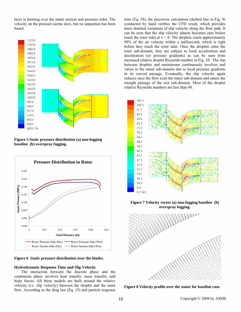
The velocity distribution in Fig. 7 shows that the inlet velocity at rotor is 52 m/s, which does not vary too much with fogging. The exit velocity at the rotor is approximately 81.7 m/s without fogging and 82 m/s with fogging. Due to increased volume flow rate from evaporated water, the exit velocity increases from 56.2 m/s without fogging to approximately 57.9 m/s. Figure 8 shows the velocity distribution over the stator in a magnified view. It is clear from the figure that a boundary
Rotor Pressure Side (Dry) Rotor Pressure Side (Wet)Rotor Suction Side (Dry) Rotor Suction Side (Wet)
Figure 6 Static pressure distribution over the blades. Hydrodynamic Response Time and Slip Velocity
The interaction between the discrete phase and the continuous phase involves heat transfer, mass transfer, and body forces. All these models are built around the relative velocity (i.e. slip velocity) between the droplet and the main flow. According to the drag law (Eq. 15) and particle response
time (Eq. 28), the piecewise calculation (dashed line in Fig. 9) conducted by hand verifies the CFD result, which provides more detailed variations of slip velocity along the flow path. It can be seen that the slip velocity almost becomes zero before reach the rotor inlet at x = 0. The droplets reach approximately 98% of the air velocity within a millisecond, which is right before they reach the rotor inlet. Once the droplets enter the rotor sub-domain, they are subject to local acceleration and deceleration (or pressure gradients) as can be seen from increased relative droplet Reynolds number in Fig. 10. The slip between droplets and mainstream continuously involves and varies in the stator sub-domain due to local pressure gradients in its curved passage. Eventually, the slip velocity again reduces once the flow exits the stator sub-domain and enters the straight passage of the exit sub-domain. Most of the droplet relative Reynolds numbers are less than 40.
Figure 11 Droplet thermal response Thermal Response Time - Theoretical calculation of
thermal response time is more complicated than the calculation of hydrodynamic response time because the temperature and velocity is coupled in Eq. (30). Equation (30) has been used for piecewise hand calculation to verify the CFD result as shown in
Fig. 11. The hand calculation shows the droplet temperature is approximately 1oC different from the mainstream flow bulk temperature before entering the rotor sub-domain; while the CFD result provides a more detailed variation of droplet temperature along the path and predicts the droplet temperature is approximately 2oC below the air temperature before reaches rotor. The hand calculation and CFD result are consistent. Relative Humidity and Liquid Concentration
The effect of liquid evaporation can be seen from the distributions of relative humidity and liquid concentration shown in Figs. 12 and 13, respectively. Low RH is seen over pressure side of both rotor and stator. Saturation is not reached at the exit. This means that the droplet thermal response time is longer than the duration of time for most of droplets flying through the entire domain. The RH is approximately 85% at the exit. The concentration of non-evaporated droplets shown in Fig. 13 is consistent with RH distribution. Also, the survived droplets at exit can be seen in Fig. 14.
Figure 12 Distribution of relative humidity (%)
Figure 13 Distribution of concentration (kg/m³) of liquid water
Breakup and Coalescence
In the present compressor stage study, the difference with and without considering breakup and coalescence is appreciable. Figure 14(a) shows droplets size distribution without considering breakup and coalescence is in a range of 10 to 25μm. Fig 14(b) shows the result without considering breakup and coalescence. It is clear from the figure that the droplets experience coalescence before they reach the rotor due to collisions induced by turbulent dispersion downstream of
sprays. The droplets reduce sizes due to evaporation before reaching the rotor, but once they enter the rotor domain, coalescence takes place and droplets size increases due to local acceleration and deceleration of the flow field.
(a)
(b) m
Figure 14 Droplet diameter (m) distribution (a) with break-up and coalescence (b) without break-up and coalescence.
Figure 15 Erosion (kg/m2s) at the leading edge of the rotor Erosion
The blade material used in the current CFD simulation is ductile metal. According to the erosion theory described earlier, the largest damage could be caused with a droplet attack angle close to 22.5°. Figure 15 shows the CFD simulated erosion rate in the rotor blade. The most eroded area is at the suction side and droplet attack angle is 30°. This deviation can be described from Figs. 14 and 15. Figure 14 shows where the droplets are accumulated and those points are marked in Fig. 15. Out of these three points, the top most point (leading edge), the angle of attack is close to 90°, the second top most point (maximum erosion point) has 30° of angle of attack and the lowest point has the angle of attack of 42°. Among these angles, 30° is closest to 22.5° and this point gives maximum erosion. The largest erosion rate is predicted as 6.15 x10⁻⁸
(kg/m2-s) or 1.93 (kg/m2-yr), which is approximately equivalent to a loss of 200 μm thickness of metal layer per year. Is this erosion serious? Probably yes if fogging is employed over the entire year. However, the current model is preliminary. It seems the model overpredicts the erosion rate. Further investigations and experimental verifications are necessary before the results can be trusted.
Figure 16 Pressure distribution at different rotor-stator relative positions.
Figure 17 Temperature distribution at different rotor-stator relative positions. Comparison of Different Rotor-Stator Relative Positions
Static pressure distribution (for overspray cases) for different rotor-stator relative positions (rotating part of the
compressor) is shown in Fig. 16. In each sub-figure, the percentage shown is the percentage of one pitch distance (0.042m) traveled by the rotor. It is found that the static pressure achieves the maximum rise at the 0% position in Fig. 16(d) because this position produces the least blockage to the airflow. On the other hand, the 75% position produces the least amount of pressure rise due to the maximum blockage. The pressure ratios at 0%, 25%, 50% and 75% position are 1.067, 1.05, 1.038 and 1.032, respectively. Temperature distribution (Fig. 17) is consistent with pressure due to air compression. Less flow blockage results in more effective compression and higher temperature. Comparison of Different Wall Boundary Conditions for Droplets
As explained before, there are three representative types of wall boundary conditions for water droplets including reflect (the droplet bounces back when it touches the wall), film (the droplet accumulates on the wall), and trap (the droplet evaporates as soon as it touches the wall). Since the trap condition will fall between the reflect and the film models, the current study conducts a comparison between using the reflect and the film boundary conditions. The comparison shows the difference at the exit of the domain is negligible (Table 1) although the wall temperature distribution in Fig. 18 shows film boundary condition makes the pressure side a bit cooler near the fore body of the airfoil. . Table 1 Comparison of different droplet wall conditions
Wall Boundary Conditions Reflect Film Inlet Static Pressure (Pa) 99656 99659 Exit Static Pressure (Pa) 105426 105466 Inlet Static Temperature (K) 300.39 300.39 Exit Static Temperature (K) 304.36 304.43 Inlet Relative Humidity (%) 100.3 100.3 Exit Relative Humidity (%) 86.5 86.2 Water Concentration at inlet (kg/m3) 0.2216 0.2314 Water Concentration at exit (kg/m3) 0.0341 0.0364
Temperature Variation on Rotor Blade
296
298
300
302
304
306
0 0.01 0.02 0.03 0.04 0.05
Axial Distance (m)
Tem
pera
ture
(K)
Pressure Side (Reflect)Pressure Side (Film)Suction Side (Reflect)Suction Side (Film)
Figure 18 Comparison of temperature distributions on the rotor wall for two different types of droplet wall boundary conditions: "Reflect" verses "Film."
It should be noted that the 2-D condition studied in this paper does not include important factors of secondary flow and
centrifugal force which will exert additional effects on the droplet dynamics. Also, the flow is subsonic. The presented results may not be representative for high-speed flows.
CONCLUSIONS CFD simulation has been performed on one rotor-stator
stage of a compressor 2-D configuration with and without fogging. The summary of the findings is:
• Under fogging, the temperature reduces, and the overall
temperature distribution in the compressor becomes more uniform. The compressor exit temperature decreases from 305.6K to 304K with 1% overspray fogging.
• Under fogging, pressure ratio rises from 1.055 to 1.058 and the axial velocity increases from 52.1 to 54.1m/s due to increased mass flow rate.
• In this study, most of the droplets reach main flow velocity (i.e. zero slip), but not main flow bulk temperature before entering the rotor passage. Local pressure gradients in both the rotor and stator flow passages drive up the droplet slip velocity during compression. Most of the droplet relative Reynolds numbers are less than 40.
• The thermal response time of the most droplets is longer than the flying time across the entire domain. The air was not saturated at exit. The average RH at exit is 85%.
• The CFD erosion model predicts that the most eroded area occurs in fore-body of the rotor suction side, corresponding to a droplet attack angle of 30°. The largest erosion rate is predicted as 6.15 x10⁻⁸ (kg/m2-s) or 1.93 (kg/m2-yr), which is approximately equivalent to a loss of 200 μm thickness of metal layer per year. The model is preliminary and further investigations are needed.
• The transient results of different rotor/stator relative positions show low air-flow blockage produces more effective compression and higher temperature rise.
• Different types droplet boundary condition shows the effect is negligible.
ACKNOWLEDGEMENT
This study was supported by the Louisiana Governor's Energy Initiative via the Clean Power and Energy Research Consortium (CPERC) and administrated by the Louisiana Board of Regents.
REFERENCES 1. Cortes, C. R. and Willems, D. E., 2003, “Gas Turbine Inlet
Air Cooling Techniques: An Overview of Current Technologies,” POWER-GEN, Las Vegas, Neva, USA.
2. Bhargava, R. and Meher-Homji, C.B., 2002, “Parametric Analysis of Existing Gas Turbines with Inlet Evaporative and Overspray Fogging,” ASME Proc. of Turbo Expo 2002, Vol. 4, pp. 387-401.
3. Chaker, M., Meher-Homji, C.B., Mee, M., 2002, “Inlet Fogging of Gas Turbine Engines - Part A: Fog Droplet Thermodynamics, Heat Transfer and Practical Considerations,” ASME Proceedings of Turbo Expo 2002, Vol. 4, pp. 413-428.
4. Chaker, M., Meher-Homji, C.B., Mee, M., 2002, “Inlet Fogging of Gas Turbine Engines - Part B: Fog Droplet Sizing Aanalysis, Nozzle Types, Measurement and
Testing,” ASME Proceedings of Turbo Expo 2002, Vol. 4, pp. 429-441.
5. Chaker, M., Meher-Homji, C.B., Mee, M., 2002, “Inlet Fogging of Gas Turbine Engines - Part C: Fog Behavior in Inlet Ducts, CFD Analysis and Wind Tunnel Experiments,” ASME Proceedings of Turbo Expo 2002, Vol. 4, pp. 443-455.
6. Payne, R. C. and White, A. J., 2007, “Three-Dimensional Calculations of Evaporative Flow in Compressor Blade Rows”, Proceedings of ASME Turbo Expo 2007, Montreal, Canada, May 14-17, 2007, ASME Paper No: GT-2007-27331.
7. Bianchi, M., Melino, F., Peretto, A., Spina, P.R. and Ingistov S., 2007, “Influence of Water Droplet Size and Temperature on Wet Compression”, Proceedings of ASME Turbo Expo 2007, Montreal, Canada, May 14-17, 2007, ASME Paper No: GT-2007-27458.
8. Zheng, Q., Shao, Y. and Zhang, Y., 2006, “Numerical Simulation of Aerodynamic Performances of Wet Compression Compressor Cascade”, ASME GT-2006-91125.
9. Li, X, and Wang, T, 2007, " Effects of Various Modelings on Mist Film Cooling," ASME Journal of Heat Transfer, vol. 129, pp. 472-482.
10. Khan, J. R. and Wang, T., 2006, “Fog and Overspray Cooling for Gas Turbine Systems with Low Calorific Value Fuels”, Proceedings of ASME Turbo Expo 2006, Barcelona, Spain, May 8-11,ASME Paper GT-2006-90396.
11. Wang, T. and Khan, J.R., 2008, “Overspray and Interstage Fog Cooling in Compressor using Stage-Stacking Scheme -- Part 1: Development of Theory and Algorithm” manuscript submitted to ASME Turbo Expo2008, Berlin, Germany, June 9-13, 2008, ASME Paper: GT-2008-50322.
12. Wang, T. and Khan, J.R., 2008, “Overspray and Interstage Fog Cooling in Compressor using Stage-Stacking Scheme -- Part 2: A Case Study” manuscript submitted to ASME Turbo Expo2008, Berlin, Germany, June 9-13, 2008, ASME Paper No: GT-2008-50323.
13. Hsu, S. T., and Wo, A. M., 1998, ‘‘Reduction of Unsteady blade Loading by Beneficial Use of Vortical and Potential Disturbances in an Axial Compressor with Rotor Clocking,’’ ASME J. Turbomach., 120, pp. 705–713.
14. Launder, B. E. and Spalding, D. B., 1972, Lectures in Mathematical Models of Turbulence, Academic Press, London, England.
15. Wolfstein, M., 1969, “The Velocity and Temperature Distribution of One-Dimensional Flow with Turbulence Augmentation and Pressure Gradient,” Int. J. Heat Mass Transfer, 12, pp. 301-318.
16. Wang, S., Liu, G., Mao, J., and Feng, Z., 2007, “Experimental Investigation on the Solid Particle Erosion in the Control Stage Nozzles of Steam Turbine” Proceedings of ASME Turbo Expo 2007, Montreal, Canada, May 14-17, 2007, ASME Paper: GT-2007-27700.
17. Schiller, L., and Naumann, A., 1933, “Uber die grundlegenden Berechnungen bei der Schwekraftaubereitung”, Zeitschrift des Vereines Deutscher Ingenieure, 77(12), 318-320.
18. Ranz, W. E. and Marshall, W. R. Jr., 1952, “Evaporation from Drops, Part I,” Chem. Eng. Prog., 48, pp. 141-146.
19. Ranz, W. E. and Marshall, W. R. Jr., 1952, “Evaporation from Drops, Part II,” Chem. Eng. Prog., 48, pp. 173-180.
20. Kuo, K. Y., 1986, Principles of Combustion, John Wiley and Sons, New York.
21. Duan, R., Koshizuka, S. and Oka, Y., 2003 “Droplet Breakup Under Impulsive Acceleration Using Moving Particle Semi-Implicit Method” 11 th International Conference on Nuclear Engineering, Tokyo, Japan, April 20-23, 2003, Paper No: ICONE11-36029.
22. O’Rourke, P. J. and Amsden, A. A., 1987, “The Tab Method for Numerical Calculation of Spray Droplet Breakup” SAE Technical Paper 872089, 1987.
23. Martula, D.S., Hasegawa, T., Lloyd, D.R. and Bionnecaze, R. T., 2000, “Coalescence-Induced Coalescence of Inviscid Droplets in a Viscous Fluid” Journal of Colloid and Interface Science 232, 241–253.
24. Pan, Y. and Suga, K., 2005, “Numerical Simulation of Binary Liquid Droplet Collision” Physics of Fluids 17, 082105.
25. Stegeman, Y.W., Chesters, A.K., vd Vosse, F.N. and Meijer, H.E.H., 1999, “Breakup of (non-) Newtonian droplets in a time-dependent elongational flow” Proceedings PPS-15, ’s-Hertogenbosch, 1999.
26. van den Hengel, E. I. V., Deen, N. G. and Kuipers, J. A. M., 2005, “Application of Coalescence and Breakup Models in a Discrete Bubble Model for Bubble Columns” Ind. Eng. Chem. Res. 2005, 44, 5233-5245.
27. Qiang, L. I., Ti-min C. A. I, Guo-qiang, H. E. and Chun-bo, H. U., 2006, “Droplet Collision and Coalescence Model” Applied Math and Mechanics, 27(1):67–73.
28. O’Rourke, P. J., 1981, “Collective Drop Effects on Vaporizing Liquid Sprays” PhD dissertation, Princeton University, , New Jersey, 1981.23.
29. Bowden, F.P. and Field, J.E., 1964, "The Brittle Fracture of Solids by Liquid Impact, by Solid Impact, and by Shock", Proceedings of the Royal Society (London) A, Vol 282, 1964, pp. 331-352.
30. Fayall, A., 1966, "Particle Aspects of Rain Erosion of Aircraft and Missiles", Philosophical Transaction of Royal Society (London) A, Vol. 260, 1966, pp. 161-167.
31. Chattopadhyay, R., 2001, Surface Wear: Analysis, Treatment, and Prevention, 2nd Ed., Chapter 2, ASM International, 2001.
32. Briscoe, B.J., Pickles, M.J., Julian K.S. and Adams M.J., 1997, “Erosion of Polymer-particle Composite Coatings by Liquid Water Jets” Wear 203-204, pp. 88-97.
33. Nokleberg, L. and Sontvedt, T., 1998, “Erosion of Oil and Gas Industry Choke Valves Using Computational Fluid Dynamics and Experiment” International Journal of Heat and Fluid Flow, 19, pp. 636-643.
34. Haugen, K., Kvernvold, O., Ronold, A. and Sandberg, R., 1995, “Sand erosion of wear-resistant materials: Erosion in choke valves” Wear 186-187, pp. 179-188.
35. Tsuji, Y. and Crowe, C.T., 1997, “Multiphase Flows with Droplets and Particles”,1st Ed.,Chap 2, 4 & 5, CRC Press.
36. Guo, T., Wang, T. and Gaddis, J. L., 2000, “Mist/Steam Cooling in a Heated Horizontal Tube – Part 2: Results and Modeling”, Transactions of the ASME, Vol. 122, 366-374.
37. Fluent Manual, Version 6.3, 2006, Fluent, Inc.