Khulna University of Engineering & Technology · Chapter 15 Control of Synchronous Motor Drives...

Chapter 15

Control of SynchronousMotor Drives

15.1 INTRODUCTION

High-power variable-speed synchronous motor drives are widely used in industry.The power rating of a large synchronous motor drive can reach 100 MW while itsvoltage can be as high as 13.8 kV [1]. The synchronous motor drive is often usedin applications where a high dynamic performance is required, such as rolling millsand mine hoists. When the synchronous motor drive is used for extruders, pumps,fans, and compressors, its variable-speed operation can provide considerable energysavings in comparison with the fixed-speed operation. Synchronous motor driveshave also found applications in the propulsion system of large vessels [2].

The synchronous motors can be controlled by various methods, including zerod-axis current (ZDC) control, maximum torque per ampere (MTPA) control, directtorque control (DTC), and power factor control (PFC). In this chapter, the dynamic andsteady-state models of the synchronous motor are introduced. The operating principleof the ZDC, MTPA, and DTC schemes for the voltage source converter (VSC) andcurrent source converter (CSC) fed synchronous motor drives is elaborated. The char-acteristics and dynamic performance of the drives employing these control schemesare analyzed. The important concepts are illustrated by computer simulations.

15.2 MODELING OF SYNCHRONOUS MOTOR

15.2.1 Construction

The synchronous motor used in high-power medium voltage (MV) drives can begenerally classified into two categories: wound rotor synchronous motor (WRSM) andpermanent magnet synchronous motor (PMSM). In the WRSM, the rotor magnetic

High-Power Converters and AC Drives, Second Edition. Bin Wu and Mehdi Narimani.© 2017 by The Institute of Electrical and Electronics Engineers, Inc. Published 2017 by John Wiley & Sons, Inc.

353

354 Chapter 15 Control of Synchronous Motor Drives

StatorStatorwinding slot

Air gap

Shaft

Rotor

Fieldwinding

Figure 15.2-1 Salient-pole WRSM (six-pole configuration).

flux is generated by the current in the rotor field winding while the PMSM usespermanent magnets to produce the rotor flux. Depending on the shape of the rotorand the distribution of the air gap along the perimeter of the rotor, the synchronousmotor can be classified into salient-pole and cylindrical (non-salient-pole) machines.

As its name indicates, the WRSM generates a rotor magnetic flux through awound rotor configuration. Figure 15.2-1 illustrates a typical six-pole WRSM. Theconstruction of the stator is similar to that of the induction motor. The rotor has afield winding, which is wound around the pole shoes. The rotor poles are positionedsymmetrically on the rotor perimeter in a radial configuration around the shaft. Theair gap is uneven in the salient-pole synchronous motors.

The rotor field winding requires direct current excitation. The rotor current can besupplied directly by brushes in contact with slip rings attached to the shaft, and theslip rings are electrically connected to the rotor winding. Alternatively, a brushlessexciter that is physically attached to the shaft can be used. The exciter generatesalternating currents that are converted into dc current for rotor winding by a dioderectifier mounted on the rotor shaft. The first option is simple, but the brushes andslip rings need regular maintenance. In contrast, the second option is more costly andcomplex, but requires little maintenance.

In PMSM, the magnetic flux of the rotor is generated by permanent magnets.Therefore, these motors are brushless. Given the lack of rotor windings, the powerdensity of the motor can be increased, which can in turn reduce the size and weightof the motor. In addition, no rotor winding losses are incurred, thereby increasing theefficiency of the motor. The main drawback of these motors is that they are expensiveand prone to demagnetization. Depending on how the permanent magnets are mountedon the rotor, the PMSM can be classified into surface-mounted and inset PM motors.

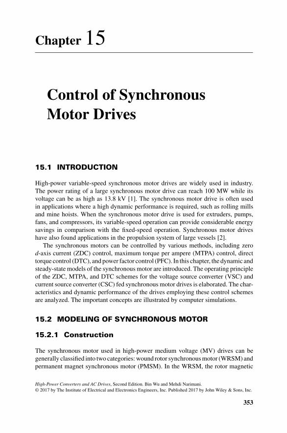
In the surface-mounted PMSM, permanent magnets are placed on the rotor surface.Figure 15.2-2 depicts such a motor, where eight magnets are mounted evenly onthe surface of the rotor core and separated by non-iron materials placed betweentwo adjacent magnets. Given that the permeability of magnets is close to that of

15.2 Modeling of Synchronous Motor 355

StatorStator

winding slot

Permanentmagnet

Shaft

Air gapS

NN

S

S

N N

S

S N

N

S

SNN

S

Rotor

Figure 15.2-2 Surface-mounted PMSM (eight-pole configuration).

non-iron materials, the effective air gap between the rotor and the stator is uniformlydistributed around the rotor surface. This type of motor is known as a cylindrical ornon-salient-pole PMSM.

The main advantage of the surface-mounted PMSM is its simplicity and lowconstruction cost in comparison with the inset PMSM. However, the magnets aresubject to centrifugal forces that may detach them from the rotor at high rotationalspeeds. Therefore, the surface-mounted PMSM is mainly for low-speed applications,where the rotor speed is up to a few thousand revolutions per minute (rpm).

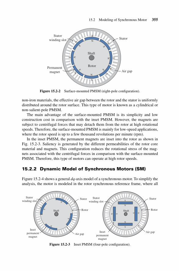
In the inset PMSM, the permanent magnets are inset into the rotor as shown inFig. 15.2-3. Saliency is generated by the different permeabilities of the rotor corematerial and magnets. This configuration reduces the rotational stress of the mag-nets associated with the centrifugal forces in comparison with the surface-mountedPMSM. Therefore, this type of motors can operate at high rotor speeds.

15.2.2 Dynamic Model of Synchronous Motors (SM)

Figure 15.2-4 shows a general dq-axis model of a synchronous motor. To simplify theanalysis, the motor is modeled in the rotor synchronous reference frame, where all

N

Shaft

N

S

N

S

S

N

S

Air gap

Stator

Rotor

Air gap

S

N

N

S

NS

N S

Shaft

Statorwinding slot

Insetpermanent

magnet

Statorwinding slot

Insetpermanent

magnet

Stator

Rotor

Figure 15.2-3 Inset PMSM (four-pole configuration).


Rsids Lls

idm

Ldmvds p

If

Stator Rotor

dsrλωRsiqs Lls

iqm

Lqmvqs

Stator

–

+

(a) d-axis circuit (b) q-axis circuit

qsrλω

λdrpλds pλds

–

+

–

+

–

+

–

++ –+–

Figure 15.2-4 General dq-axis model of a synchronous motor in the rotor synchronousreference frame.

the variables are of dc quantities. The stator circuit of the dq-axis model is essentiallythe same as that of the induction motor (IM) model shown in Fig. 14.3.3 with thefollowing modifications:

� The speed of the arbitrary reference frame 𝜔 in the IM model is replaced withthe rotor speed 𝜔r in the rotor synchronous frame.

� The magnetizing inductance Lm is replaced with the dq-axis magnetizing induc-tances Ldm and Lqm of the synchronous motor. In a cylindrical synchronousmotor, the dq-axis magnetizing inductances are equal (Ldm = Lqm) whereas inthe salient-pole motors, the d-axis magnetizing inductance is normally lowerthan the q-axis magnetizing inductance (Ldm < Lqm).

To model the rotor circuit, the field current in the rotor winding of a WRSM isrepresented by a constant current source If in the d-axis circuit as shown in 15.2-4a[2]. In the PMSM, the permanent magnets that replace the field winding in the WRSMcan be modeled by an equivalent current source If with a fixed magnitude.

To simplify the synchronous motor model presented in Fig. 15.2-4, the followingmathematical manipulations can be performed. The stator voltage equations for themotor can be expressed as

{vds = Rsids − 𝜔r𝜆qs + p𝜆ds

vqs = Rsiqs + 𝜔r𝜆ds + p𝜆qs(15.2-1)

where 𝜆ds and 𝜆qs are the d- and q-axis stator flux linkages, respectively, which aregiven by

{𝜆ds = Llsids + Ldm(If + ids) = Ldids + 𝜆r

𝜆qs = (Lls + Lqm)iqs = Lqiqs(15.2-2)


ωrLqiqs

Ld

λ

Lq

(a) d-axis circuit (b) q-axis circuit

iqs Rsiqs Rs

vqsvds

+–ωrLdids ωr r

+ –+ –+

–

+

–

Figure 15.2-5 Simplified dq-axis model of a synchronous motor in the rotor synchronousreference frame.

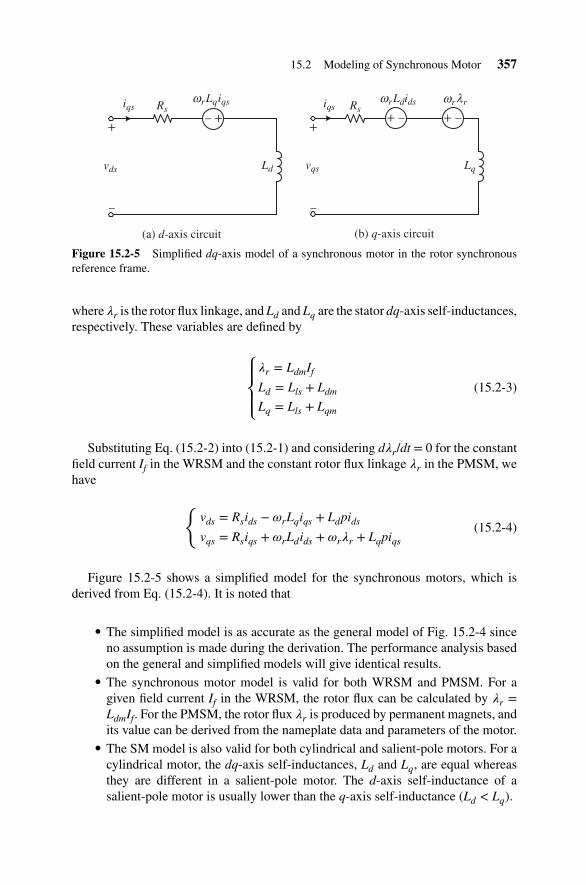
where 𝜆r is the rotor flux linkage, and Ld and Lq are the stator dq-axis self-inductances,respectively. These variables are defined by

⎧⎪⎨⎪⎩𝜆r = LdmIf

Ld = Lls + Ldm

Lq = Lls + Lqm

(15.2-3)

Substituting Eq. (15.2-2) into (15.2-1) and considering d𝜆r/dt = 0 for the constantfield current If in the WRSM and the constant rotor flux linkage 𝜆r in the PMSM, wehave

{vds = Rsids − 𝜔rLqiqs + Ldpids

vqs = Rsiqs + 𝜔rLdids + 𝜔r𝜆r + Lqpiqs(15.2-4)

Figure 15.2-5 shows a simplified model for the synchronous motors, which isderived from Eq. (15.2-4). It is noted that

� The simplified model is as accurate as the general model of Fig. 15.2-4 sinceno assumption is made during the derivation. The performance analysis basedon the general and simplified models will give identical results.

� The synchronous motor model is valid for both WRSM and PMSM. For agiven field current If in the WRSM, the rotor flux can be calculated by 𝜆r =LdmIf. For the PMSM, the rotor flux 𝜆r is produced by permanent magnets, andits value can be derived from the nameplate data and parameters of the motor.

� The SM model is also valid for both cylindrical and salient-pole motors. For acylindrical motor, the dq-axis self-inductances, Ld and Lq, are equal whereasthey are different in a salient-pole motor. The d-axis self-inductance of asalient-pole motor is usually lower than the q-axis self-inductance (Ld < Lq).


The electromagnetic torque produced by a synchronous motor can be calculatedwith the same equation for the induction motor given in Eq. 14.3-8, that is,

Te =3P2

(iqs𝜆ds − ids𝜆qs) (15.2-5)

Substituting Eq. (15.2-2) into (15.2-5), we obtain

Te =3P2

[𝜆r iqs + (Ld − Lq) idsiqs] (15.2-6)

The rotor speed 𝜔r is governed by the motion equation, namely,

𝜔r =PJS

(Te − Tl) (15.2-7)

where P is the number of pole pairs, J is the moment of inertia of the rotor and itsmechanical load, S is the Laplace operator, and Tl is the load torque.

To derive the synchronous motor model for computer simulation, Eq. (15.2-4) canbe rearranged as follows:

⎧⎪⎨⎪⎩ids =

1S

(vds − Rsids + 𝜔rLqiqs)∕Ld

iqs =1S

(vqs − Rsiqs − 𝜔rLdids − 𝜔r𝜆r)∕Lq

(15.2-8)

where the differential operator p in Eq. (15.2-4) is replaced by Laplace operator S.The block diagram for the dynamic simulation of a synchronous motor is shown

in Fig. 15.2-6, which is derived from Eqs. (15.2-6) to (15.2-8). The input variablesof the synchronous motor model are the dq-axis stator voltages vds and vqs, the rotorflux linkage 𝜆r, and the mechanical load Tl. The output variables are the dq-axisstator currents ids and iqs, the rotor speed 𝜔r, and the electromagnetic torque Te ofthe motor.

15.2.3 Steady-State Equivalent Circuits

The steady-state model of a synchronous motor provides a useful tool to analyze thesteady-state operation of the motor. The steady-state model can be developed fromthe dynamic model shown in Fig. 15.2-5. Considering that the dq-axis stator currents,ids and iqs, in the rotor synchronous reference frame are of constant dc values insteady state, their derivatives in Eq. (15.2-4), pids and piqs, become zero. Therefore,


1/Ldids

−

+−

−

1/Lq

Rs

3P/2

λr

iqs

Te

vqs

vds

+

+

−Rs

Tl

×

×

× +

+

Ld ids

Lq iqs

×

–

×

×

λrωr

ωrLqiqs

Lq ids iqs

iqs + Ld ids iqs

rλ

Eq. (15.2–8) Eq. (15.2–6) Eq. (15.2-7)

ids

iqs

1s

1s

PJs

Te

ωr

ωrLdids

ωr

+

–

+

ωr

Figure 15.2-6 Block diagram for the dynamic simulation of synchronous motors.

the equations that describe the steady-state characteristics of the synchronous motorare given by

{vds = Rsids − 𝜔rLqiqs

vqs = Rsiqs + 𝜔rLdids + 𝜔r𝜆r(15.2-9)

Based on Eq. (15.2-9), a steady-state model for the synchronous motor can bederived, which is illustrated in Fig. 15.2-7 for steady-state analysis.

ω LqiqsRsλ

Rs

(a) d-axis circuit

+

–

(b) q-axis circuit

iqsids

vqsvds

r ω Ldidsr ωr r

+

–

+ – + –+–

Figure 15.2-7 Steady-state model of a synchronous motor.


15.3 VSC FED SM DRIVE WITH ZERO d-AXISCURRENT (ZDC) CONTROL

15.3.1 Introduction

The synchronous motor can be controlled by a number of methods to achieve differentobjectives [3]. For instance, the d-axis stator current of the motor can be set to zeroduring the operation to simplify control scheme design and implementation. In thissection, the ZDC control scheme is introduced and analyzed.

15.3.2 Principle of ZDC Control

The ZDC control can be realized by resolving the three-phase stator current in thestationary reference frame into dq-axis components in the synchronous referenceframe. The d-axis component ids is then kept at zero by the controller [4]. With theZDC, the stator current is is equal to its q-axis component iqs, that is,

⎧⎪⎨⎪⎩i⃗s = ids + jiqs = jiqs

is =√

i2ds + i2qs = iqs

for ids = 0 (15.3-1)

where i⃗s is the space vector of the stator current, and is represents its magnitude, whichis also the peak value of the three-phase stator current in the stationary referenceframe.

The electromagnetic torque of the motor

Te =32

P(𝜆r iqs + (Ld − Lq) idsiqs) (15.3-2)

can then be simplified to

Te =32

P𝜆riqs =32

P𝜆ris (15.3-3)

The above equation indicates that when ids = 0, the motor torque is proportionalto the stator current is. With a constant rotor flux linkage 𝜆r, the torque exhibitsa linear relationship with the stator current. This is similar to torque productionin a dc machine with a constant field current, where the electromagnetic torque isproportional to the armature current.

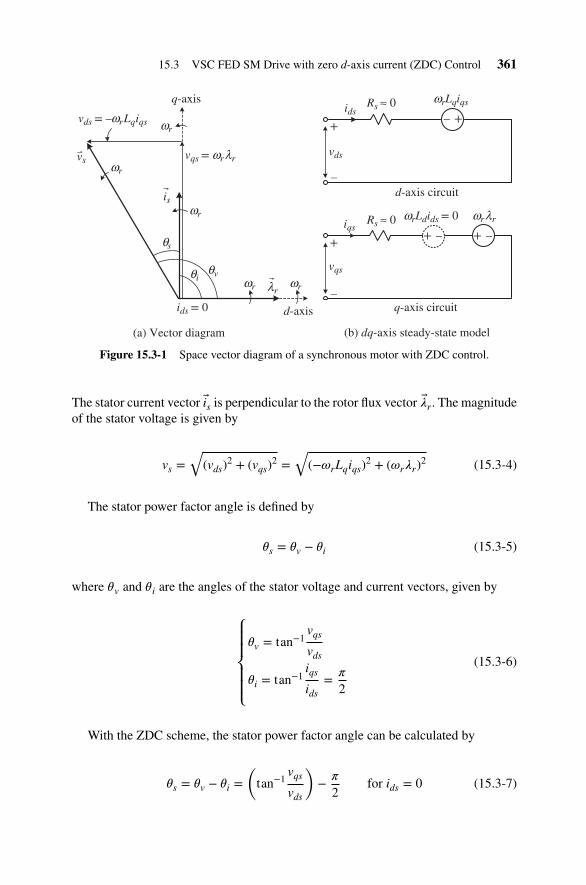
A space vector diagram for a synchronous motor with the ZDC control is illustratedin Fig. 15.3-1. The vector diagram is derived according to the SM steady-state modelunder the assumption that the stator winding resistance Rs is negligibly small and therotor flux linkage vector 𝜆r is aligned with the d-axis of the synchronous referenceframe. All the vectors in the diagram rotate in space at the rotor synchronous speed.

15.3 VSC FED SM Drive with zero d-axis current (ZDC) Control 361

Lqiqs

d-axis

q-axis

vds = –ωr

vqs =

ids = 0

(a) Vector diagram (b) dq-axis steady-state model

iqs

ids

d-axis circuit

q-axis circuit

Rs ≈ 0

vds

vqs

ωrλr

ωr

vsωr

isωr

θs

θiθv

ωr λrωr

+

–

ωrLdids = 0 ωrλr

ωrLqiqsRs ≈ 0

+

–

+ – + –

+–

Figure 15.3-1 Space vector diagram of a synchronous motor with ZDC control.

The stator current vector i⃗s is perpendicular to the rotor flux vector 𝜆r. The magnitudeof the stator voltage is given by

vs =√

(vds)2 + (vqs)

2 =√

(−𝜔rLqiqs)2 + (𝜔r𝜆r)

2 (15.3-4)

The stator power factor angle is defined by

𝜃s = 𝜃v − 𝜃i (15.3-5)

where 𝜃v and 𝜃i are the angles of the stator voltage and current vectors, given by

⎧⎪⎪⎨⎪⎪⎩

𝜃v = tan−1vqs

vds

𝜃i = tan−1iqs

ids= 𝜋

2

(15.3-6)

With the ZDC scheme, the stator power factor angle can be calculated by

𝜃s = 𝜃v − 𝜃i =(tan−1

vqs

vds

)− 𝜋

2for ids = 0 (15.3-7)


PWM

PI

PI

vdc

vs

3L-VSI

C

CylindricalPMSM

= 0

dq/abc abc/dq

PWM

PI

Lg

(vqg = 0)

–1.5 vdg

vdc

vi

3L-VSRGrid

~

abc/dq dq/abc

vg ig

vdg

θgθg

idg

iqg*

*

*vdi*vqi

Qg*

vdc*

vag,vbg

iag,ibg

idg, iqg

ias,ibs

vai,vbi,vci

θr

ids

iqs*

*

ids

Te*

is

*** vas,vbs,vcs***

÷

PI*

r1.5P1

ωr

ωr

ωr, θr

iqg

PI

PI

idg

ids iqsvds*vqs

*

iqs

θg

detector

Load

λ+–

+–

+–

+–

+–

+

–

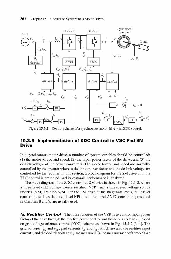
Figure 15.3-2 Control scheme of a synchronous motor drive with ZDC control.

15.3.3 Implementation of ZDC Control in VSC Fed SMDrive

In a synchronous motor drive, a number of system variables should be controlled:(1) the motor torque and speed, (2) the input power factor of the drive, and (3) thedc-link voltage of the power converters. The motor torque and speed are normallycontrolled by the inverter whereas the input power factor and the dc-link voltage arecontrolled by the rectifier. In this section, a block diagram for the SM drive with theZDC control is presented, and its dynamic performance is analyzed.

The block diagram of the ZDC controlled SM drive is shown in Fig. 15.3-2, wherea three-level (3L) voltage source rectifier (VSR) and a three-level voltage sourceinverter (VSI) are employed. For the SM drive at the megawatt levels, multilevelconverters, such as the three-level NPC and three-level ANPC converters presentedin Chapters 8 and 9, are usually used.

(a) Rectifier Control The main function of the VSR is to control input powerfactor of the drive through the reactive power control and the dc bus voltage vdc basedon grid voltage oriented control (VOC) scheme as shown in Fig. 15.3-2 [3, 4]. Thegrid voltages vag and vbg, grid currents iag and ibg, which are also the rectifier inputcurrents, and the dc-link voltage vdc are measured. In the measurement of three-phase


variables, we only need to measure two of them since the third one can be calculatedfrom xa + xb + xc = 0 in a three-phase balanced system.

To realize the grid VOC, the grid voltage angle 𝜃g is detected. This angle is usedfor the transformation of variables from the abc stationary frame to the dq rotatingreference frame through the abc/dq transformation or from the rotating frame backto the stationary frame through the dq/abc transformation as shown in Fig. 15.3-2.With the grid VOC, the speed of the dq-axis rotating frame is given by 𝜔g = 2𝜋fg,where fg is the grid frequency.

To find the grid voltage angle 𝜃g, the grid phase voltages, vag and vbg, are measuredand transformed to the 𝛼𝛽 frame through the abc/𝛼𝛽 transformation presented inChapter 14.

⎧⎪⎪⎨⎪⎪⎩

v𝛼g = 23

(vag −

12

vbg −12

vcg

)= vag

v𝛽g = 23

(√3

2vbg −

√3

2vcg

)=

√3

3(vag + 2vbg)

for vag + vbg + vcg = 0

(15.3-8)

The grid voltage angle 𝜃g and its peak value vg can then be found from

⎧⎪⎨⎪⎩𝜃g = tan−1

v𝛽g

v𝛼g

vg =√

(v𝛼g)2 + (v𝛽g)2

(15.3-9)

There are three feedback control loops in the system: two inner current loops forthe control of the dq-axis currents idg and iqg, and one outer dc voltage feedback loopfor the control of the dc-link voltage vdc. The measured three-phase grid currents inthe abc stationary frame iag, ibg, and icg are transformed to the dq-axis currents idgand iqg in the dq rotating frame, which represent the active and reactive componentsof the three-phase grid current in the VOC scheme, respectively.

With the VOC scheme, the grid voltage vector is aligned with the d-axis of therotating reference frame. In doing so, the q-axis component of the grid voltage, vqg, isequal to zero and its d-axis component is equal to the magnitude of the grid voltage,

that is, vqg = 0 and vdg =√

v2g − v2

qg = vg. As a result, the calculation of the active

and reactive grid power can be simplified as

⎧⎪⎨⎪⎩Pg = 3

2(vdgidg + vqgiqg) = 3

2vdgidg

Qg = 32

(vqgidg − vdgiqg) = −32

vdgiqg

for vqg = 0 (15.3-10)


from which the q-axis current reference can be calculated by

i∗qg =Q∗

g

−1.5vdg(15.3-11)

where Q∗g is the reactive power reference, which can be set to zero for unity power

factor operation, a positive value for leading power factor operation, or a negativevalue for lagging power factor operation. To control the reactive power accurately,the measured dq-axis current iqg is compared with its reference i∗qg, and the error issent to the q-axis current PI controller to generate the q-axis voltage reference v∗qi forthe rectifier, as shown in Fig. 15.3-2.

To control the dc-link voltage tightly, the measured dc-link voltage vdc is comparedwith its reference v∗dc, and the error is sent to the dc-link voltage PI controller, whichgenerates the d-axis current reference i∗dg. Compared with the measured d-axis currentidg, the difference between i∗dg and idg is sent to the d-axis current PI controller, whichgenerates the d-axis voltage reference v∗di for the rectifier.

The dq-axis voltage references v∗di and v∗qi in the dq-axis rotating frame, whichare of dc quantity, are then transformed into three-phase reference voltages v∗ai, v∗bi,and v∗ci in the abc stationary frame via the dq/abc transformation, which are sent tothe PWM generator. The three-phase reference voltages are sinusoidal waveforms,based on which a carrier-based modulation or space vector modulation (SVM) canbe employed to generate gate signals for the switching devices in the rectifier, whichcontrols its reactive power and dc-link voltage according to their respective references.

(b) Inverter Control The main function of the VSI is to control the torque andspeed of the motor while its d-axis stator current is set to zero to achieve ZDC control.This is implemented by three feedback loops: two inner loops for the dq-axis statorcurrents ids and iqs, and one outer loop for the rotor speed 𝜔r as shown in Fig. 15.3-2.

To control the speed of the motor, the rotor speed𝜔r is detected, which is comparedwith its reference 𝜔∗

r . The error is sent to the speed PI controller, which generatesthe torque reference T∗

e . The reference for the q-axis stator current i∗qs, which isthe torque-producing component of the stator current, is calculated according to thetorque equation of (15.3-3). The d-axis stator current reference i∗ds is set to zero.

The measured dq-axis stator currents, ids and iqs, are then compared with theirreferences i∗ds and i∗qs. The errors are sent to two PI controllers, which generate thedq-axis voltage references v∗ds and v∗qs for the inverter. These two references in thesynchronous frame are then transformed into three-phase voltage references v∗as, v∗bs,and v∗cs in the stationary frame via the dq/abc transformation. For the reference frametransformation between the dq-axis rotor synchronous frame and the abc stationaryframe, the rotor position angle 𝜃r is needed, which is detected by an encoder mountedon the rotor shaft as shown in Fig. 15.3-2.

The three-phase voltage references v∗as, v∗bs, and v∗cs are then sent to the PWM gen-erator. Either carrier-based modulation or space vector modulation can be employedto generate gate signals for the switching devices in the inverter, which controls thed-axis stator current ids and the rotor speed𝜔r according to their respective references.


Table 15.3-1 System Parameters of a 2.45 MW VSC Fed Drive

PMSM 2.45 MW/4000 V/53.33 Hz/400 rpm/490 ACylindrical machine

Control scheme Zero d-axis current (ZDC) scheme

System input variables d-axis stator current: i∗ds = 0

Rotor speed reference: 𝜔∗r (step input)

Rectifier reactive power reference: Q∗g = 0

dc-link voltage reference: v∗dc = 7045 V (3.05 pu)

Rectifier Topology: three-level NPC converter

Modulation scheme: SVM

Switching frequency: 740 Hz

Filter inductance Lg: 0.775 mH (0.045 pu)

Inverter Topology: three-level NPC converter

Modulation scheme: SVM

Switching frequency: 740 Hz

Harmonic filter: No

dc-link filter Capacitor: 2500 μF (4.0 pu)

Grid voltage/frequency 4000 V/60 Hz

15.3.4 Transient Analysis

The dynamic performance of a synchronous motor drive using three-level VSCs withthe ZDC scheme is investigated through computer simulation. A 2.45 MW cylindricalPMSM is used in the investigation and its parameters are given in Table A-1 at theend of this chapter. The drive system parameters are listed in Table 15.3-1.

Figure 15.3-3 shows the start-up transient response of the 2.45 MW SM drive withthe ZDC scheme. A three-level neutral point clamped (3L-NPC) converter is used inthe rectifier and inverter, and both converters are modulated by a conventional SVMscheme. The device switching frequency is 740 Hz, which leads to an equivalentswitching frequency of 1480 Hz for both converters due to the three-level convertertopology.

The rotor speed reference 𝜔∗r has a step input from zero to its rated value of 1 pu at

t= 0.05 s. The motor accelerates under the no-load condition while its torque is limitedto the rated value set by the saturation level of the speed PI controller. Due to the ZDCcontrol scheme, the d-axis stator current ids is kept at zero while the q-axis iqs, which isthe torque-producing component of the stator current, is proportional to the torque Te.The peak value of the phase-a stator current ias is equal to iqs with the ZDC scheme.The dc-link voltage vdc is maintained around its reference value, which is 3.05 pu.

It is noted that when the drive is operating in steady state under no-load conditions,after the startup, the stator current ias (and also iqs) is very low. This is mainly due to


0 0.05 0.10 0.15 0.20 0.25 0.30 0.35

iasiqs

ids

t (s)

(pu)rω

ias, ids, iqs (pu)

Te (pu)

vdc (pu)

rω*rω

0

0.5

1.0

–1.5

0

1.5

0

0.5

1.0

2.5

3.0

3.5

Figure 15.3-3 Start-up transient of a 2.45 MWSM drive with ZDC scheme.

the fact that the rotating field in the air gap of the PMSM is produced by the permanentmagnets. A small stator current is provided to cover the stator winding losses andsmall rotational losses (windage and friction). This is not like the induction motors,where a much higher stator current is needed to produce a rotating field in the air gapeven though the motor is running in steady state under no-load conditions. In largeinduction motors, the no-load stator current would be in the range of 0.25 to 0.3 pu,which corresponds to the magnetizing inductance of 4.0 to 3.0 pu, respectively.

It is also noted that in order to reduce the drive start-up time in the simulation, themoment of inertia of the motor is reduced on purpose such that the drive can startwithin a short period of time. In practice, it takes longer time to start, especially whenthe drive starts under the loaded conditions.

Figure 15.3-4 shows the transient response of the 2.45 MW drive to a step changein the load torque. The motor operates initially at its rated speed of 400 rpm (1 pu)under the no-load conditions. A step load torque of 1 pu is applied to the motor at t =0.1 s. The d-axis current ids is kept around zero by the ZDC scheme, and its q-axiscurrent iqs is proportional to the torque Te. The motor speed 𝜔∗

r is kept at the ratedvalue of 1 pu except at the moment when the load torque is applied. The dc-linkvoltage is maintained around its reference value of 3.05 pu.

15.4 VSC FED SM Drive with MTPA Control 367

0.9

0.95

1.0

1.05

0 0.05 0.10 0.15 0.20 0.25 0.30 0.35 t (s)

–1.5

0

1.5

0

0.5

1.0

2.5

3.0

3.5

iasiqsids

Tl Te

ias, ids, iqs (pu)

Te (pu)

vdc (pu)

*rω

rω

(pu)rω

Figure 15.3-4 Response of a 2.45 MW SM drive to a step load torque change (ZDC scheme).

15.4 VSC FED SM DRIVE WITH MTPA CONTROL

15.4.1 Introduction

In addition to the ZDC control scheme presented in the preceding section, the syn-chronous motor can also be controlled by maximum torque per ampere (MTPA)scheme, where the motor torque can be produced by a minimum stator current [3–6].With this approach, the power losses in the stator winding and also in the powerconverters can be minimized, which improves the efficiency of the drive system. Inthis section, the MTPA control method is presented and analyzed.

15.4.2 Principle of MTPA Control

As discussed earlier, the electromagnetic torque of a synchronous motor can becalculated by

Te =32

P(𝜆r iqs + (Ld − Lq) idsiqs) (15.4-1)


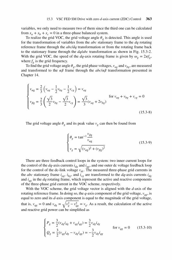
The above equation indicates that the motor torque is a function of dq-axis statorcurrents ids and iqs. By adjusting the ratio of ids to iqs, it is possible to produce a giventorque by a minimum stator current. For a given stator current

is =√

i2ds + i2qs (15.4-2)

its d-axis component can be calculated by

ids =√

i2s − i2qs (15.4-3)

Substituting the above equation into the torque equation of (15.4-1), the electro-magnetic torque of the motor can be rewritten as

Te =32

P(𝜆r iqs + (Ld − Lq)

(√i2s − i2qs

)iqs

)(15.4-4)

In a cylindrical motor, the dq-axis self-inductances, Ld and Lq, are equal. Theabove torque equation is simplified to

Te =32

P𝜆riqs (15.4-5)

where the motor torque is proportional to the q-axis stator current iqs, but it is notaffected by the d-axis stator current ids. To achieve the MTPA control in a cylindricalmotor drive, we can set the d-axis current ids to zero. In doing so, the motor torque isproduced by a minimum stator current (is = iqs). To summarize, the MTPA controlfor a cylindrical motor is essentially the ZDC control.

In a salient-pole motor, the principle of the MTPA scheme can be illustratedthrough the following derivations. By differentiating the torque equation of (15.4-4)with respect to iqs, we have

dTe

diqs= 3P

2

⎛⎜⎜⎜⎝𝜆r + (Ld − Lq) ids − (Ld − Lq) i2qs

1√i2s − i2qs

⎞⎟⎟⎟⎠(15.4-6)

To achieve the MTPA operation, the above equation is set to zero

𝜆r + (Ld − Lq) ids − (Ld − Lq)i2qs

ids= 0 (15.4-7)

from which the d-axis stator current is given by

ids =−𝜆r

2(Ld − Lq)±

√√√√ 𝜆2r

4(Ld − Lq)2+ i2qs for Ld ≠ Lq (15.4-8)


iqs

Rsids

d-axis

≈

≈

circuit

q-axis circuit

vds

vqs

ωr Lq iqs

ωr λrωr Ld ids

(b)

–

– –

–

–

++ +

++

dq-axis steady-state model

0

Rs 0

(a) Vector diagram

d-axis

q-axis

vds = –ωr Lq iqs ωr λr

iqs

ids

is

ωr Ld ids

vqs =ωr Ld ids + ωr λr

λr

vs

θi

θv

ωr

ωr

θs

ωr

Figure 15.4-1 Space vector diagram of a synchronous motor with MTPA control.

The d-axis stator current shown in the above equation has two possible values.The first term on the right side of the equation has a positive value because the d-axisself-inductance Ld of a salient-pole synchronous motor is normally lower than theq-axis self-inductance Lq. To minimize the d-axis stator current for the MTPA control,the second term should have a negative value, that is,

ids =−𝜆r

2(Ld − Lq)−

√√√√ 𝜆2r

4(Ld − Lq)2+ i2qs for Ld ≠ Lq (15.4-9)

The space vector diagram of a synchronous motor with the MTPA control is givenin Fig. 15.4-1a, which is derived according to its dq-axis steady-state model givenin Fig. 15.4-1b. The equations for the calculations of stator voltage angle 𝜃v, statorcurrent angle 𝜃i, and stator power factor angle 𝜃s are the same as those given in theZDC scheme, and therefore are not repeated here. The main difference between thevector diagrams of the two schemes is that the stator current angle 𝜃i for the ZDCscheme is equal to 𝜋/2 whereas it varies with the operating conditions in the MTPAscheme. It is noted that the d-axis stator current ids is negative, which is caused bythe negative value of the d-axis stator voltage vds. Equation (15.4-9) also shows thatthe d-axis current is negative since the second term on the right side of the equationhas a higher value than the first term.

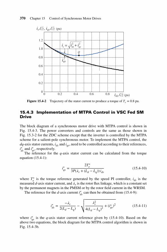
Figure 15.4-2 shows an example of the variation of the stator current is with itsd-axis current ids for a given torque of Te = 0.8 pu. Different combinations of thedq-axis stator currents ids and iqs can produce the same required torque, but theminimum stator current takes place at point Q, at which the MTPA operation isachieved.


Q

0 0.2 0.4 0.6 0.80

0.2

0.4

0.6

0.8

1.0

1.2

ids / (pu)2

22qsdss iii

is / , iqs / (pu)

i

= +

qs

2 2

Figure 15.4-2 Trajectory of the stator current to produce a torque of Te = 0.8 pu.

15.4.3 Implementation of MTPA Control in VSC Fed SMDrive

The block diagram of a synchronous motor drive with MTPA control is shown inFig. 15.4-3. The power converters and controls are the same as those shown inFig. 15.3-2 for the ZDC scheme except that the inverter is controlled by the MTPAscheme for a salient-pole synchronous motor. To implement the MTPA control, thedq-axis stator currents, ids and iqs, need to be controlled according to their references,i∗ds and i∗qs, respectively.

The reference for the q-axis stator current can be calculated from the torqueequation (15.4-1):

i∗qs =2T∗

e

3P(𝜆r + (Ld − Lq)) ids(15.4-10)

where T∗e is the torque reference generated by the speed PI controller, ids is the

measured d-axis stator current, and 𝜆r is the rotor flux linkage, which is a constant setby the permanent magnets in the PMSM or by the rotor field current in the WRSM.

The reference for the d-axis current i∗ds can then be obtained from (15.4-9):

i∗ds =−𝜆r

2(Ld − Lq)−

√√√√ 𝜆2r

4(Ld − Lq)2+ (i∗qs)

2 (15.4-11)

where i∗qs is the q-axis stator current reference given by (15.4-10). Based on theabove two equations, the block diagram for the MTPA control algorithm is shown inFig. 15.4-3b.


PWM

vdc

3L-VSI

C

Salient-polePMSM

PWM

Lg vi

3L-VSR

abc/dq dq/abc

ig

θg

vag,vbg

iag,ibg

idg, iqg

ias,ibs

vai,vbi,vci*** vas,vbs,vcs

***

is

ωr, θr

PI

(vqg = 0)

–1.5

÷

vdg

vdc

vdg

idg

iqg*

*

*vdi*vqi

Qg*

vdc*

iqg

PI

PI++ +

+

–– –

+

+

–

–

–

idg

Eq (15.4–10)

Eq (15.4–11)ids

iqs*

*

(a) System block diagram

Te*

(b) MTPA control

dq/abc abc/dq

θr

ids iqsvds*vqs

*

PI

*

ωr

ωrMTPA

control

Te*

ids

Speed PIcontroller

vs

ids

iqs

PIiqs

*

ids

PIids

*

Grid

~vg

θg

θg

detector

Load

Figure 15.4-3 Block diagram of a salient-pole PMSM drive with MTPA control.


The dynamic performance of a synchronous motor drive with the MTPA scheme isinvestigated by computer simulation. The drive system parameters are the same asthose given in Table 15.3-1 except that the d-axis current reference is no longer to bezero; it varies with the operating conditions of the drive. A salient-pole synchronousmotor of 2.5 MW is used in the study, and its nameplate data and motor parametersare given in Table A-2 at the end of this chapter.

Figure 15.4-4 shows the dynamic response of the SM drive with MTPA controlduring the system start-up followed by a sudden change in load torque. The speedreference 𝜔∗

r has a step increase from zero to the rated value at t = 0.1 s. Themotor accelerates under the no-load condition, and its torque is limited to 1.3 puby the speed PI controller. The rotor speed 𝜔r increases linearly with time due to


0

0.5

1.0

–2.0

0

2.0

0

0.5

1.0

0 0.25 0.5 0.75 1.0 1.25 1.5 1.75

2.5

3.0

3.5

*r r

(pu)r

i

ω

ω ω

as, ids, iqs (pu)

iasiqs

ids

Te (pu)

vdc (pu)

t (s)0.1

ias

iqs

ids

Figure 15.4-4 Transient response of a salient-pole SM drive with MTPA control.

the constant torque operation during the startup transient. When the rotor speed 𝜔rreaches its reference at approximately t = 0.6 s, its torque drops to zero.

At t = 1.0 s, a rated load torque is applied to the motor. The motor torque Teresponds quickly and increases to the rated value as well. Both dq-axis stator currentsvary accordingly such that magnitude of the stator current is minimized by the MTPAscheme to minimize the stator winding and converter power losses. The dc-linkvoltage is maintained around the set value of 3.05 pu by the rectifier.

15.5 VSC FED SM DRIVE WITH DTC SCHEME

15.5.1 Introduction

The DTC is another advanced control scheme developed for motor drives for appli-cations where a high dynamic performance is required [6, 7]. The principle of theDTC scheme was introduced in Chapter 14, but it was for induction motor (IM)drives using two-level VCSs (2L-VSC). In this section, the principle of DTC forsynchronous motor drives using three-level NPC converters is introduced, and itsdynamic performance is investigated.

15.5 VSC FED SM Drive with DTC Scheme 373

15.5.2 Principle of DTC

The electromagnetic torque of a synchronous motor can be expressed by

Te =3P2𝜆s𝜆r sin 𝜃T (15.5-1)

where 𝜃T is the torque angle, which is the angle between the stator flux linkage vector𝜆s and the rotor flux linkage vector 𝜆r.To realize the DTC control, the magnitudeof the stator flux 𝜆s is kept constant (normally at its rated value) by the controller,and the motor torque Te can then be controlled by 𝜃T directly. This method is,therefore, referred to as the DTC. With the magnitude of the stator flux kept constant,the magnitude of the rotor flux 𝜆r is almost constant since the difference betweenthe stator and rotor fluxes is only the leakage flux produced by the stator leakageinductance.

From the synchronous motor model developed in the earlier section, the stator fluxvector 𝜆s can be mainly determined by the stator voltage:

p𝜆s = v⃗s − Rsi⃗s (15.5-2)

where Rs is the stator winding resistance, which is quite small, especially in largesynchronous motors. The above equation indicates that the derivative of 𝜆s reactsinstantly to the changes in v⃗s. As discussed in Chapter 14, the stator voltage v⃗s can becontrolled by the reference vector V⃗ref in the space vector modulation scheme. Since

the reference vector V⃗ref can be synthesized by the voltage vectors of the inverter, the

magnitude and angle of the stator flux vector 𝜆s can be adjusted by proper selectionof the inverter voltage vectors.

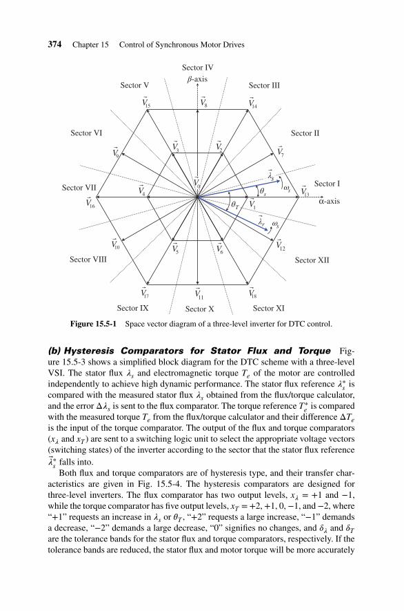
(a) Space Vector Diagram Figure 15.5-1 shows the space vector diagram ofa three-level VSI for the DTC control. There are 19 space vectors, V⃗0 to V⃗18, whichwere defined in Table 8.3.1 in Chapter 8. To realize the DTC control, the space vectordiagram is divided into 12 sectors from I to XXII. The stator flux vector 𝜆s, rotor fluxvector 𝜆r, and torque angle 𝜃T are also shown in the figure. Both stator and rotor fluxvectors are rotating in space at the synchronous speed 𝜔s.

Figure 15.5-2 illustrates the impact of the selection of the voltage vectors on 𝜆s

and 𝜃T . Assuming the stator flux vector 𝜆s is in Sector I, selection of voltage vectorV⃗7 will make both 𝜆s and 𝜃T increase as shown in Fig. 15.5-2a, while selection of V⃗12will make 𝜆s increase and 𝜃T decrease as shown in Fig. 15.5-2b. Similarly, selection ofV⃗10 will make both 𝜆s and 𝜃T decrease whereas selection of V⃗9 will make 𝜆s decreaseand 𝜃T increase. It can be concluded from the above analysis that the magnitude ofthe stator flux 𝜆s and the torque angle 𝜃T can be fully adjusted by selection of propervoltage vectors of the inverter.


Sector I

Sector II

Sector III

Sector IV

Sector V

Sector VI

Sector VIII

Sector IX Sector X Sector XI

Sector XII

α-axiss

s

β-axis

T 1

23

4 13

1817

16

15 14

12

11

10

9

8

7

65

0Sector VII

V V V

VV V

V

V

VVVV

V

VV

V

V V V

λ

θ sω

rλsω

θ

Figure 15.5-1 Space vector diagram of a three-level inverter for DTC control.

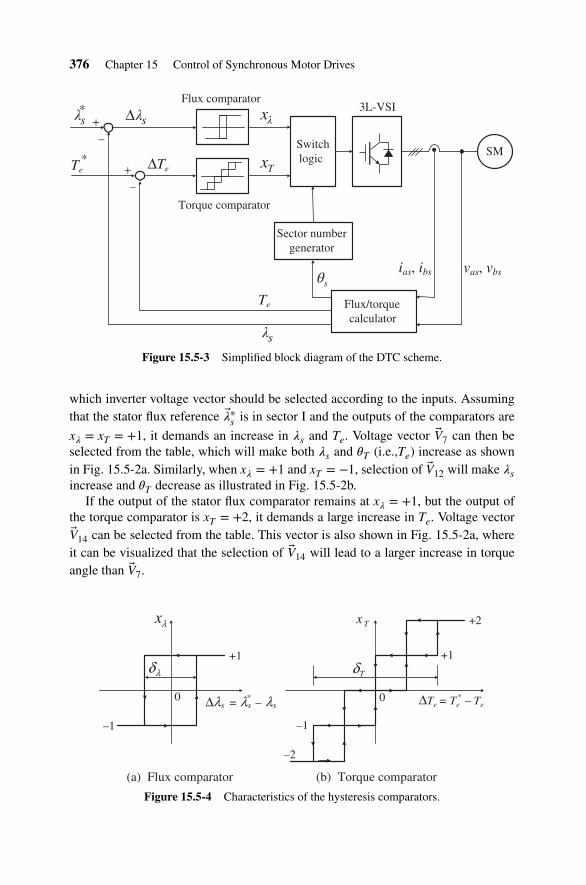
(b) Hysteresis Comparators for Stator Flux and Torque Fig-ure 15.5-3 shows a simplified block diagram for the DTC scheme with a three-levelVSI. The stator flux 𝜆s and electromagnetic torque Te of the motor are controlledindependently to achieve high dynamic performance. The stator flux reference 𝜆∗s iscompared with the measured stator flux 𝜆s obtained from the flux/torque calculator,and the error Δ𝜆s is sent to the flux comparator. The torque reference T∗

e is comparedwith the measured torque Te from the flux/torque calculator and their difference ΔTeis the input of the torque comparator. The output of the flux and torque comparators(x𝜆 and xT ) are sent to a switching logic unit to select the appropriate voltage vectors(switching states) of the inverter according to the sector that the stator flux reference𝜆∗s falls into.

Both flux and torque comparators are of hysteresis type, and their transfer char-acteristics are given in Fig. 15.5-4. The hysteresis comparators are designed forthree-level inverters. The flux comparator has two output levels, x𝜆 = +1 and −1,while the torque comparator has five output levels, xT =+2, +1, 0, −1, and −2, where“+1” requests an increase in 𝜆s or 𝜃T , “+2” requests a large increase, “−1” demandsa decrease, “−2” demands a large decrease, “0” signifies no changes, and 𝛿𝜆 and 𝛿Tare the tolerance bands for the stator flux and torque comparators, respectively. If thetolerance bands are reduced, the stator flux and motor torque will be more accurately


Sector I

Sector II

Sector XII

α-axis

2

18

14

12

7

6

tΔ7

′13

Δt12

(a) Selection of Vector7

(b) Selection of Vector12

Sector I

Sector II

Sector XII

α-axis

2

18

14

12

7

6

′

′

0

10

9≈

≈

10

9

≈≈

0

V

V

V

V

V

V

V

V

VV

V

V

V

V V

V

V

V

V

V

V

V

V

Tθ Tθ

rλ

sλ

sλ

sλ

sλ

rλ

′Tθ Tθ

Figure 15.5-2 Impact of voltage vector selection on 𝜆s and 𝜃T .

controlled with less ripples but this is at the expense of higher switching frequenciesfor the inverter, and vice versa.

(c) Switching Logic Table 15.5-1 presents the switching logic for the statorflux reference 𝜆∗s that rotates in the counter clockwise direction in space [7, 8]. Theinput variables of the table are x𝜆, xT , and the sector number while its output indicates


3L-VSI

SMSwitchlogic

Flux/torquecalculator

Sector numbergenerator

*s

*

Δ

ΔTe

x

Tx

Flux comparator

Torque comparator

vas, vbsias, ibs

λ sλ λ

sθ

+–

+–

sλ

Te

Te

Figure 15.5-3 Simplified block diagram of the DTC scheme.

which inverter voltage vector should be selected according to the inputs. Assumingthat the stator flux reference 𝜆∗s is in sector I and the outputs of the comparators are

x𝜆 = xT = +1, it demands an increase in 𝜆s and Te. Voltage vector V⃗7 can then beselected from the table, which will make both 𝜆s and 𝜃T (i.e.,Te) increase as shownin Fig. 15.5-2a. Similarly, when x𝜆 = +1 and xT = −1, selection of V⃗12 will make 𝜆sincrease and 𝜃T decrease as illustrated in Fig. 15.5-2b.

If the output of the stator flux comparator remains at x𝜆 = +1, but the output ofthe torque comparator is xT = +2, it demands a large increase in Te. Voltage vectorV⃗14 can be selected from the table. This vector is also shown in Fig. 15.5-2a, whereit can be visualized that the selection of V⃗14 will lead to a larger increase in torqueangle than V⃗7.

+1

–1

0

+1

–1

0

λx Tx

sss λλλ –=Δ * Te – Te=ΔTe*

λδ Tδ

(a) Flux comparator (b) Torque comparator

+2

–2

Figure 15.5-4 Characteristics of the hysteresis comparators.


Table 15.5-1 DTC Switching Logic for a Three-Level Voltage Source Inverter

ComparatorOutput

Sector Number

x𝜆 xT I II III IV V VI VII VIII IX X XI XII

+1

+2 V⃗14 V⃗8 V⃗15 V⃗9 V⃗16 V⃗10 V⃗17 V⃗11 V⃗18 V⃗12 V⃗13 V⃗7

+1 V⃗7 V⃗14 V⃗8 V⃗15 V⃗9 V⃗16 V⃗10 V⃗17 V⃗11 V⃗18 V⃗12 V⃗13

0 V⃗0 V⃗0 V⃗0 V⃗0 V⃗0 V⃗0 V⃗0 V⃗0 V⃗0 V⃗0 V⃗0 V⃗0

−1 V⃗12 V⃗13 V⃗7 V⃗14 V⃗8 V⃗15 V⃗9 V⃗16 V⃗10 V⃗17 V⃗11 V⃗18

−2 V⃗18 V⃗12 V⃗13 V⃗7 V⃗14 V⃗8 V⃗15 V⃗9 V⃗16 V⃗10 V⃗17 V⃗11

−1

+2 V⃗15 V⃗9 V⃗16 V⃗10 V⃗17 V⃗11 V⃗18 V⃗12 V⃗13 V⃗7 V⃗14 V⃗8

+1 V⃗9 V⃗16 V⃗10 V⃗17 V⃗11 V⃗18 V⃗12 V⃗13 V⃗7 V⃗14 V⃗8 V⃗15

0 V⃗0 V⃗0 V⃗0 V⃗0 V⃗0 V⃗0 V⃗0 V⃗0 V⃗0 V⃗0 V⃗0 V⃗0

−1 V⃗10 V⃗17 V⃗11 V⃗18 V⃗12 V⃗13 V⃗7 V⃗14 V⃗8 V⃗15 V⃗9 V⃗16

−2 V⃗17 V⃗11 V⃗18 V⃗12 V⃗13 V⃗7 V⃗14 V⃗8 V⃗15 V⃗9 V⃗16 V⃗10

When the output of the torque comparator xT is zero (no need to adjust Te), zerovector V⃗0 can be selected from Table 15.5-1. The switching logic for all 12 sectorsfrom I to XII is summarized in Table 15.5-1.

It is noted that the switching logic presented in Table 15.5-1 is not unique. Forexample, when x𝜆 = +1 and xT = ±1, the selection of the small vectors V⃗2 and V⃗6

instead of the medium vectors V⃗7 and V⃗12 is also valid. However, the selection of thesmall vectors may slow down the system dynamic response due to the shorter length(lower voltage) of these vectors than the medium vectors, but it may result in lowerharmonic distortion in the inverter output voltages.

(d) Stator Flux and Torque Calculator Similar to the DTC scheme forthe induction motor drive presented in Chapter 14, the stator flux vector 𝜆s of thesynchronous motor can be expressed as

𝜆s = 𝜆ds + j𝜆qs

=∫

(vds − Rsids)dt + j∫

(vqs − Rsiqs)dt(15.5-3)

from which the magnitude and angle of the stator flux linkage vector can beobtained by

⎧⎪⎨⎪⎩𝜆s =

√𝜆2

ds + 𝜆2qs

𝜃s = tan−1

(𝜆qs

𝜆ds

) (15.5-4)


The dq-axis stator voltages and currents in Eq. (15.5-3); vds, vqs, ids, and iqs, can becalculated from the measured three-phase stator voltages and currents. The developedelectromagnetic torque can be determined by

Te =3P2

(iqs𝜆ds − ids𝜆qs) (15.5-5)

The above equations illustrate that the stator flux 𝜆s, the stator flux angle 𝜃s, andthe developed torque Te can all be obtained from the measured stator voltages andcurrents. The only motor parameter required in the calculations is the stator resistanceRs, which is easy to measure and its value does not vary with the operating conditionsof the motor too much.

The stator flux vector 𝜆s of a synchronous motor can also be calculated from Eq.(15.2-2), which is

𝜆s = 𝜆ds + j𝜆qs = (Ldids + 𝜆r) + j(Lqiqs) (15.5-6)

Compared with Eq. (15.5-3), the above question does not required integrators tofind the stator flux linkage, but need the motor dq-axis inductances and rotor fluxlinkage in the calculation.

15.5.3 Implementation of DTC Control in VSC Fed SMDrive

Figure 15.5-5 shows the block diagram of a synchronous motor drive with the DTCcontrol scheme, where the rectifier with its control is omitted since it has beendiscussed in the earlier sections. The dc-link voltage is kept constant by the rectifierwhile the motor torque and speed are controlled by the inverter with the DTC scheme.

The control block diagram of Fig. 15.5-5 is essentially the same as that given inFig. 15.5-3 except that a motor speed feedback control is added. As discussed earlier,the essence of the DTC control is to keep the stator flux 𝜆s constant and control thetorque Te independently. This is achieved by the stator flux and torque comparators,whose outputs are sent to the switching logic unit to generate switching signals forthe inverter. The drive system with the DTC scheme has the following features:

� There is only one PI controller for the motor speed control, but no PI controllersare needed for the stator flux or torque control.

� There is no need for PWM schemes such as carrier-based or space vectormodulation. The gate signals for the inverter are directly generated by theswitching logic.

� There is no need for reference frame transformation between the abc stationaryframe and the dq rotating frame.


vdc

3L-VSI

C

Non-salientPMSM

is

ωr,θr

vas,vbs ias,ibs

ias, ibs

vas, vbs

vs

Flux/torquecalculator

sθ

Sector numbergenerator

PI

*

ωr

ωr

Flux comparator

Torque comparator*eT

*sλ

eTsλ

sλΔ

eΔT

Fromrectifier

λx

Tx

Mechanicalload

Switchlogic

Table 15.5–1

+

–

+–

+–

+–

Figure 15.5-5 Block diagram of a synchronous motor drive with DTC control.

Therefore, the DTC scheme is simpler than the ZDC and MTPA schemes whileits dynamic performance is comparable due to the decoupled stator flux and torquecontrol.


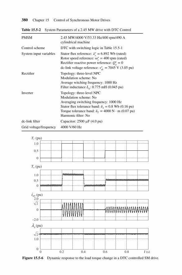
The performance of the DTC scheme for a synchronous motor drive is investigated bycomputer simulation. The parameters of the drive system are given in Table 15.5-2.A 2.45 MW cylindrical PMSM is used in the investigation, and its parameters arelisted in Table A-1 at the end of this chapter.

Figure 15.5-6 shows the dynamic response of the DTC controlled drive to thestep changes in the load torque. The drive initially operates at its rated speed ofnr = 400 rpm under the no-load condition. The load torque Tl is suddenly increasedto its rated value of 1.0 pu at t = 0.2 s, decreased to zero at t = 0.4 s, and finallyincreased to 0.5 pu at 0.6 s. It can be observed that the motor torque Te respondsquickly and follows the load torque profile closely. The torque ripple is set by thetorque tolerance band 𝛿T . The phase-a stator current ias varies with Te accordingly.


Table 15.5-2 System Parameters of a 2.45 MW drive with DTC Control

PMSM 2.45 MW/4000 V/53.33 Hz/400 rpm/490 Acylindrical machine

Control scheme DTC with switching logic in Table 15.5-1

System input variables Stator flux reference: 𝜆∗s = 6.892 Wb (rated)Rotor speed reference: 𝜔∗

r = 400 rpm (rated)Rectifier reactive power reference: Q∗

g = 0dc-link voltage reference: v∗dc = 7045 V (3.05 pu)

Rectifier Topology: three-level NPCModulation scheme: NoAverage witching frequency: 1000 HzFilter inductance Lg: 0.775 mH (0.045 pu)

Inverter Topology: three-level NPCModulation scheme: NoAveraging switching frequency: 1000 HzStator flux tolerance band: 𝛿𝜆 = 0.8 Wb (0.16 pu)Torque tolerance band: 𝛿T = 4000 N ⋅ m (0.07 pu)Harmonic filter: No

dc-link filter Capacitor: 2500 μF (4.0 pu)


(pu)sλ

t (s)

0

0.5

1.0

–2.0

0

2.0

0

1.0

0 0.2 0.4 0.6 0.8

Tl (pu)

Te (pu)

ias (pu)

0

0.5

1.0

2

2

Figure 15.5-6 Dynamic response to the load torque change in a DTC controlled SM drive.

15.6 Control of CSC FED SM Drives 381

The stator flux 𝜆s is kept constant by the stator flux comparator. No obviousdisturbances can be observed from the stator flux waveform during the sudden changesin the load torque. This is due to the fact that the stator flux is calculated by 𝜆s =∫ (vds − Rsids)dt + j ∫ (vqs − Rsiqs)dt, where the stator winding resistance Rs is quitesmall, especially for large-size synchronous motors. In addition, the integral functionin the stator flux calculation can be considered as a low-pass filter. As a result, asudden change in the stator current due to the load torque change does not producenoticeable variations in the stator flux waveform.

15.6 CONTROL OF CSC FED SM DRIVES

15.6.1 Introduction

The CSC fed synchronous motor drives have found various applications in industry.Figure 15.6-1 shows the typical configuration of a PWM CSC fed synchronous motordrive, where a current source rectifier (CSR) and a current source inverter (CSI) areused. The two converters are linked by a dc inductor Ldc, which makes the dc-linkcurrent smooth and continuous.

SM

dcL PWM CSIPWM CSR

Grid

(a) Schematic diagram

(b) Simplified block diagram

CSR CSI

Grid

SM

Cf

CfCg

Cg

dcL

isiw

ic

vsiwgig vg vdcr

idc

vdci

Lg

Lg

+

–

+

–

Figure 15.6-1 Configuration of a PWM CSC fed synchronous motor drive.


The CSC fed SM drive is characterized by a simple converter topology, inherentfour-quadrant operation, and reliable fuseless short-circuit protection. In VSC fedMV drives, both inverter output voltage and frequency are controlled by the inverterPWM scheme. In contrast, in CSC fed drives, the magnitude of the inverter outputcurrent is controlled by the dc-link current idc produced by the rectifier whereasthe output frequency of the inverter is controlled by the inverter PWM scheme. Inaddition, the stator current of the motor is not directly controlled by the inverter due tothe presence of the filter capacitor Cf between the inverter and the motor. Therefore,additional measures are required to control the CSC fed drives.

The control schemes presented in the earlier sections for the VSC fed synchronousmotor drives can also be applied to the CSC fed SM drives, including the ZDC controland MTPA control. This section presents both ZDC and MTPA control methods forthe CSC fed synchronous motor drives.

15.6.2 CSC Fed SM Drive with ZDC Control

(a) Inverter Control To facilitate the analysis of the CSC fed synchronousmotor drive with the ZDC control scheme, a space vector diagram for the drive isshown in Fig. 15.6-2. The rotor rotates in space at the synchronous speed 𝜔r. Therotor axis is aligned with the d-axis of the synchronous reference frame. With theZDC control where the d-axis current ids is zero, the stator current vector i⃗s is alignedwith the q-axis of the synchronous frame, and its magnitude is equal to the q-axiscurrent iqs. The stator voltage vector v⃗s leads its current vector i⃗s by 𝜃s, which is

the stator power factor angle. The capacitor current i⃗c leads v⃗s by 𝜋∕2. The inverterPWM current i⃗w is a vector sum of i⃗s and i⃗c, and its angle with respect to the d-axis ofthe synchronous frame is 𝜃w, which can be calculated by 𝜃w = tan−1(iqw∕idw). FromFig. 15.6-2, the inverter firing angle can be calculated by

𝜃inv = 𝜃w + 𝜃r (15.6-1)

where 𝜃r is the rotor position angle.

Stator

d-axis

q-axis

rω

rθ

sλ

wθ

invθ

ic

ic

is = iqs (ids = 0)

iw

vs

Rotor

rλrω

rωrω

sθ

ZDC scheme

Figure 15.6-2 Vector diagram for a CSC fed SM drive with ZDC control.


PIEq.

(15.6–5)

*

ids = 0

iqs*

ωr

ωr

*

Cartesian topolar

iqw*

idw*

θr

θw

θinv

PWM(SHE)

CSICylindrical

PMSM

PWM(SHE)

Lg iwg

CSRGrid

~ vgig is

Ldc

vdcr vdci

Cg

iw

Cf

ic

idc

PI

idc*

vdcr*

cos–1

θrecθg

vag,vbg

vg

/

1.5 mmax

yxy x

θwg

vG

Capacitor voltagedetector

idc

iCg

Capacitorcompensator

θ

idc

ωr, θr

Load

+

–

+

–

+

+–

+

–+

–+

Figure 15.6-3 Block diagram of a CSC fed SM drive with ZDC scheme.

The block diagram of a CSC fed SM drive with the ZDC scheme is shown inFig. 15.6-3, where the rectifier controls the dc-link current and the inverter controlsthe motor speed. To minimize the harmonic distortion in the rectifier input and inverteroutput currents, selective harmonic elimination (SHE) modulation scheme is used forboth converters. The modulation index of the SHE scheme is fixed at its maximumvalue. The rectifier and the inverter are controlled by their firing angles 𝜃rec and 𝜃inv,respectively.

To achieve the ZDC control, the d-axis stator current reference i∗ds is set to zero,and its q-axis stator current reference i∗qs is set by the speed PI controller as shown inFig. 15.6-3. The PI controller compares the measured rotor speed𝜔r with its reference𝜔∗

r and makes the rotor speed follow its reference closely. The inverter output currentiw is a sum of the filter capacitor current ic and stator current is. The dq-axis inverteroutput currents can be calculated by

{idw = icd + ids = −𝜔rCf vqs + ids

iqw = icq + iqs = 𝜔rCf vds + iqs(15.6-2)

where icd and icq are the dq-axis filter capacitor currents, given by

{icd = −𝜔rCf vqs

icq = 𝜔rCf vds(15.6-3)

Note that the derivative terms associated with the capacitor current are not includedin the above equation for simplicity since these terms have little impact on the dynamicperformance of the drive.


The dq-axis inverter output currents in Eq. (15.6-2) are a function of both dq-axisstator voltages and currents. By substituting the dq-axis stator voltage equations of(15.2-9) into (15.6-2), the inverter dq-axis output currents are a function of the statorcurrent only:

{idw = −𝜔2

r Cf 𝜆r − 𝜔2r Cf Ldids + ids

iqw = −𝜔2r Cf Lqiqs + iqs

(15.6-4)

where the stator winding resistance is omitted for simplicity. Equation (15.6-4) canbe used to serve as the inverter output current references i∗dw and i∗qw with the filtercapacitor current taking into account:

{i∗dw = −𝜔2

r Cf 𝜆r + (1 − 𝜔2r Cf Ld)i∗ds

i∗qw = (1 − 𝜔2r Cf Lq) i∗qs

(15.6-5)

Equation (15.6-5) is implemented in the control scheme of Fig. 15.6-3 as thecapacitor compensator block.

With the cartesian to polar coordinates conversion, the inverter output currentreferences i∗dw and i∗qw can be converted to the dc-link current reference i∗dc andinverter output current angle 𝜃w, given by

⎧⎪⎪⎨⎪⎪⎩

𝜃w = tan−1

(i∗qw

i∗dw

)

i∗dc =√

(i∗dw)2 + (i∗qw)2

(15.6-6)

The inverter firing angle 𝜃inv can then be calculated from Eq. (15.6-1), which is𝜃inv = 𝜃w + 𝜃r.

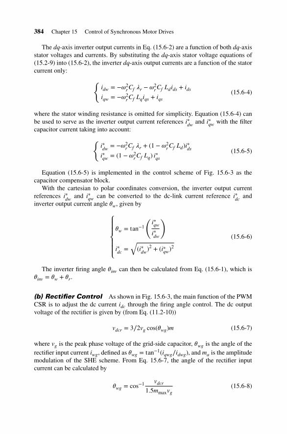
(b) Rectifier Control As shown in Fig. 15.6-3, the main function of the PWMCSR is to adjust the dc current idc through the firing angle control. The dc outputvoltage of the rectifier is given by (from Eq. (11.2-10))

vdcr = 3∕2vg cos(𝜃wg)m (15.6-7)

where vg is the peak phase voltage of the grid-side capacitor, 𝜃wg is the angle of therectifier input current iwg, defined as 𝜃wg = tan−1(iqwg∕idwg), and ma is the amplitudemodulation of the SHE scheme. From Eq. 15.6-7, the angle of the rectifier inputcurrent can be calculated by

𝜃wg = cos−1 vdcr

1.5mmaxvg(15.6-8)


d-axis

q-axis

gθ

wgθ

recθ

iwg

vg

gω

gω

ωg

iCg

iCgig

a-axis(Stationary frame)

idwgiqwg

Figure 15.6-4 Vector diagram of the rectifier with firing angle control.

where mmax is the maximum modulation index, which is between 0.98 and 1.1,depending on the number of harmonics to be eliminated. The above equation isimplemented in the rectifier control scheme shown in Fig. 15.6-3.

The relationship among the rectifier input current angle 𝜃wg, the grid-side capacitorvoltage angle 𝜃g, and the rectifier firing angle 𝜃rec is illustrated in a vector diagramof Fig. 15.6-4. Similar to the grid VOC discussed in Section 15.3, the grid-sidecapacitor voltage vector v⃗g, which is also the rectifier input voltage vector, is alignedwith the d-axis of a rotating reference frame. The rotating reference frame rotatesin space at a speed given by 𝜔g = 2𝜋 fg, where fg is the frequency of the grid. With

the delay angle control, the rectifier input current i⃗wg lags its input voltage v⃗g by

𝜃wg. The capacitor current i⃗Cg leads v⃗g by 𝜋/2. The grid current i⃗g is the sum of

i⃗wg and i⃗Cg as shown in Fig. 15.6-4. The rectifier firing angle can then be obtainedfrom

𝜃rec = 𝜃g − 𝜃wg (15.6-9)

To detect the grid-side capacitor voltage, its phase voltages, vag and vbg, aremeasured. The measured capacitor voltages are sent to the capacitor voltage detector,which calculates the magnitude of the grid-side capacitor voltage vg, and its angle𝜃g. The algorithm for the capacitor voltage detector is the same as that given in Eq.(15.3-9) and thus is not repeated here.

It is noted that with the firing angle control only (no modulation index control),the rectifier input power factor is not controllable. However, the lagging reactivecomponent of the rectifier input current (iqwg) compensates the leading reactivecurrent (iCg) produced by the grid-side capacitor, which improves the overall inputpower factor of the drive system as shown in Fig. 15.6-4. For the full control ofthe rectifier input power factor, the control scheme for the PWM CSR presented inChapter 11 can be considered.


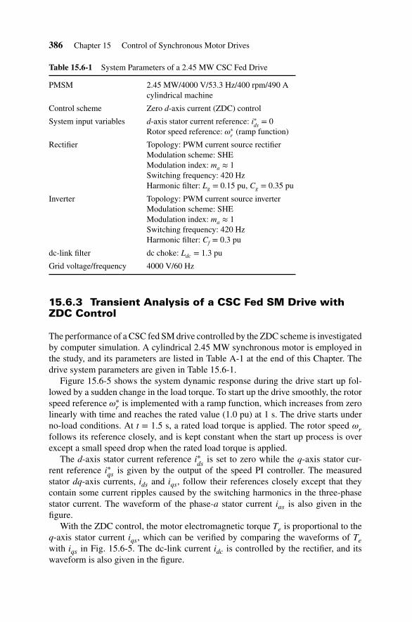
Table 15.6-1 System Parameters of a 2.45 MW CSC Fed Drive

PMSM 2.45 MW/4000 V/53.3 Hz/400 rpm/490 Acylindrical machine

Control scheme Zero d-axis current (ZDC) control

System input variables d-axis stator current reference: i∗ds = 0Rotor speed reference: 𝜔∗

r (ramp function)

Rectifier Topology: PWM current source rectifierModulation scheme: SHEModulation index: ma ≈ 1Switching frequency: 420 HzHarmonic filter: Lg = 0.15 pu, Cg = 0.35 pu

Inverter Topology: PWM current source inverterModulation scheme: SHEModulation index: ma ≈ 1Switching frequency: 420 HzHarmonic filter: Cf = 0.3 pu

dc-link filter dc choke: Ldc = 1.3 pu


15.6.3 Transient Analysis of a CSC Fed SM Drive withZDC Control

The performance of a CSC fed SM drive controlled by the ZDC scheme is investigatedby computer simulation. A cylindrical 2.45 MW synchronous motor is employed inthe study, and its parameters are listed in Table A-1 at the end of this Chapter. Thedrive system parameters are given in Table 15.6-1.

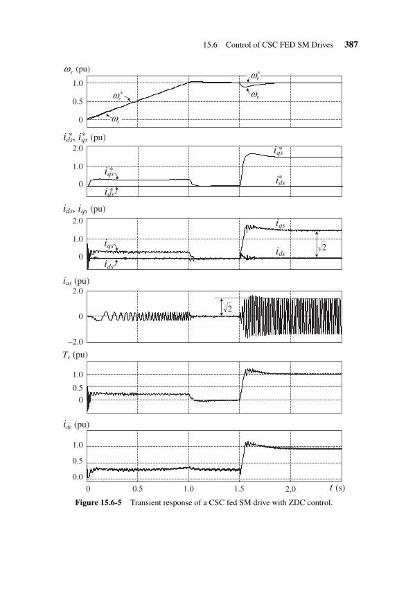
Figure 15.6-5 shows the system dynamic response during the drive start up fol-lowed by a sudden change in the load torque. To start up the drive smoothly, the rotorspeed reference 𝜔∗

r is implemented with a ramp function, which increases from zerolinearly with time and reaches the rated value (1.0 pu) at 1 s. The drive starts underno-load conditions. At t = 1.5 s, a rated load torque is applied. The rotor speed 𝜔rfollows its reference closely, and is kept constant when the start up process is overexcept a small speed drop when the rated load torque is applied.

The d-axis stator current reference i∗ds is set to zero while the q-axis stator cur-rent reference i∗qs is given by the output of the speed PI controller. The measuredstator dq-axis currents, ids and iqs, follow their references closely except that theycontain some current ripples caused by the switching harmonics in the three-phasestator current. The waveform of the phase-a stator current ias is also given in thefigure.

With the ZDC control, the motor electromagnetic torque Te is proportional to theq-axis stator current iqs, which can be verified by comparing the waveforms of Tewith iqs in Fig. 15.6-5. The dc-link current idc is controlled by the rectifier, and itswaveform is also given in the figure.


0

0.5

1.0

0

1.0

2.0

rω

(pu)rω

0

0.5

1.0

Te (pu)

0

1.0

2.0

iqsids

ids, iqs (pu)

ids, iqs (pu)

* *

ids

iqs

iqs

ids

ids

iqs

*

*

*

*

rω

rω

*rω

*

0 0.5 1.0 1.5

0.0

0.5

1.0

idc (pu)

2.0 t (s)

–2.0

0

2.0ias (pu)

2

2

Figure 15.6-5 Transient response of a CSC fed SM drive with ZDC control.


PIEq.

(15.6–5)

*

ωr

ωr

Capacitorcompensator

Cartesian topolar

iqw*

idw*

θr

θw

θinv

PWM(SHE)

CSISalient-pole

PMSM

FromCSR

is Mechanicalload

ωr, θr

Ldc

vdcr vdciiw

Cf

ic

idc

PIidc*vdcr

*θ

idc

MTPAcontrol

iqs*

ids* Eq.

(15.6–10)

Te*

To CSRcontroller

Refer toFig. 15.6–3

θr

ias,ibs

ids iqs

abc/dq

ids

+ +

– –

+–

+

+

+–

Figure 15.6-6 Block diagram of a CSC fed SM drive with MTPA scheme.

It is noted that when the drive is operating in steady state during 1.2 s < t <1.5 s under no-load conditions, the stator current ias is quite small. This phenomenonhas been explained in Section 15.3.4, and is not repeated here. However, the dc-linkcurrent idc is not significantly reduced during this period. It mainly flows through thefilter capacitor Cf at the output of the inverter, but the average dc-link voltage is quitelow. The dc-link power in this case is equal to the sum of the inverter power lossesand motor power losses including copper, iron, and rotational losses.

15.6.4 CSC Fed SM Drive with MTPA Control

The MTPA control presented in the earlier sections for the VSC fed drive can beequally applied to the CSC fed drive. Figure 15.6-6 shows the block diagram of aCSC fed drive with the MTPA control. The block diagram is essentially the same asthat for the CSC fed drive with the ZDC control in Fig. 15.6-3 except that an MTPAblock is added to the system. The essence of the MTPA control is to adjust the dq-axisstator currents separately to produce a given torque with a minimal stator current.The algorithm for the MTPA control was developed earlier, and is given here for thepurpose of convenience:

⎧⎪⎪⎨⎪⎪⎩

i∗qs =2T∗

e

3P(𝜆r + (Ld − Lq)) ids

i∗ds =−𝜆r

2(Ld − Lq)−

√√√√ 𝜆2r

4(Ld − Lq)2+ (i∗qs)

2

(15.6-10)


0

0.5

1.0 *rω rω

(pu)rω

–2.0

2.0iqs

ids

0

0.5

1.0

Te (pu)

ids, iqs (pu)

–2.0

0

2.0ias (pu)

0 0.5 1.0 1.5 2.0 t (s)

2

iqs

ids

rω

0

Figure 15.6-7 Transient response of a CSC fed SM drive with MTPA control.

The dynamic performance of the CSC fed SM drive with the MTPA control isinvestigated by computer simulation. The drive system parameters are the same asthose given in Table 15.6-1 except that the d-axis current reference i∗ds is no longer tobe zero; it varies with the operating conditions of the drive. A 2.5 MW salient-polesynchronous motor is used in the study, and its parameters are given in Table A-2 atthe end of this chapter.

Figure 15.6-7 shows the dynamic response of the drive during the system start upfollowed by a sudden change in load torque. To start up the drive smoothly, the rotorspeed reference 𝜔∗

r is increased linearly with time from zero to the rated value att = 1.0 s. The rotor speed 𝜔r follows its reference closely. At t = 1.5 s, a rated loadtorque is applied to the motor, and the motor torque Te increases accordingly. Withthe MTPA control, both dq-axis stator currents ids and iqs vary accordingly such thatthe magnitude of the stator current is is minimized under any operating conditions.The motor torque Te is produced by both ids and iqs, and it is no longer proportionalto iqs as in the case of the ZDC control. The d-axis stator current ids has a negativevalue as discussed in Section 15.4.2.


15.7 SUMMARY

This chapter focuses on the control schemes for the synchronous motor drives. Thechapter starts with the dynamic and steady-state models for the synchronous motorsin the rotor synchronous frame, which are generalized models suitable for both woundrotor and PMSMs. They are also applicable to salient-pole and cylindrical motors.

A number of control schemes are introduced for the synchronous motor drives,including the ZDC, MTPA control, and DTC. The operating principle of theseschemes is analyzed, and their implementation in VSC and CSC fed synchronousmotor drives is discussed. The drive system dynamic performance is illustrated withcomputer simulations. The synchronous motor drive with the ZDC control featureslinear torque–current characteristics and easy controller design. The drive with theMTPA scheme benefits from reduced power losses in the motor and power converterswhile the DTC controlled drive has the advantage of simple control scheme and easyimplementation.

REFERENCES

1. R. Bhatia, H.U. Krattiger, A. Bonanini, et al., “Adjustable speed drive with a single 100-MWsynchronous motor,” ABB Review, no. 6, pp. 14–20, 1998.

2. “Synchronous Motors - High Performance in all Applications,” ABB Product Brochure, 20pages, 2011.

3. B.K. Bose, Power Electronics and Motor Drives: Advances and Trends, Academic Press,2006.

4. P.C. Sen, Principle of Electric Machines and Power Electronics, 3rd Edition, Wiley, 2013.

5. C.T Pan and S. M. Sue, “A linear maximum torque per ampere control for IPMSM drivesover full-speed range,” IEEE Transactions on Energy Conversion, vol. 20, no. 2, pp. 359–366, 2005.

6. B. Wu, Y. Lang, N. Zargari, and S. Kouro, Power Conversion and Control of Wind EnergySystems, Wiley/IEEE Press, 2011.

7. M. Kadjoudj, S. Taibi, N. Golea, and H. Benbouzid, “Modified direct torque control ofpermanent magnet synchronous motor drives,” International Journal of Sciences and Tech-niques of Automatic Control and Computer Engineering, vol. 1, no. 2, pp. 167–180, 2007.

8. A. Damiano, G. Gatto, I. Marongiu, and A. Perfetto, “An Improved Multilevel DTC Drive,”IEEE Power Electronics Specialists Conference, pp. 1452–1457, 2011.

Appendix 391

APPENDIX

Table A-1 2.45 MW/4000 V/53.3 Hz Cylindrical PMSM

Motor Ratings Motor Parameters

Rated output power 2.45 MW Stator resistance, Rs 24.21 mΩRated line-to-line voltage 4000 V d-axis synchronous inductance, Ld 9.816 mHRated stator current 490 A q-axis synchronous inductance, Lq 9.816 mHRated speed 400 rpm Rated stator frequency 53.33 HzRated torque 58.5 kN ⋅ m Rated power factor 0.716Rated rotor flux linkage 4.97 Wb Number of pole pairs 8Moment of inertia 312 kg ⋅ m2

Table A-2 2.5 MW/4000 V/40 Hz Salient-Pole PMSM

Motor Ratings Motor Parameters

Rated output power 2.5 MW Stator resistance, Rs 24.25 mΩRated line-to-line voltage 4000 V d-axis synchronous inductance, Ld 8.9995 mHRated stator current 485 A q-axis synchronous inductance, Lq 21.8463 mHRated speed 400 rpm Rated stator frequency 40 HzRated torque 59.7 kN ⋅ m Rated power factor 0.739Rated rotor lux linkage 4.76 Wb Number of pole pairs 6Moment of inertia 420 kg ⋅ m2

Date post:	08-Jul-2020
Category:	Documents
Upload:	others
View:	6 times
Download:	0 times

Khulna University of Engineering & Technology · Chapter 15 Control of Synchronous Motor Drives...

Documents