Kill Zone Analysis for a Bank-to-Turn Missile-Target Engagement by Venkatraman Renganathan A Thesis Presented in Partial Fulfillment of the Requirements for the Degree Master of Science Approved July 2016 by the Graduate Supervisory Committee: Armando A. Rodriguez, Chair Panagiotis Artemiadis Spring Melody Berman ARIZONA STATE UNIVERSITY August 2016
Transcript
Kill Zone Analysis for a Bank-to-Turn
Missile-Target Engagement
by
Venkatraman Renganathan
A Thesis Presented in Partial Fulfillmentof the Requirements for the Degree
Master of Science
Approved July 2016 by theGraduate Supervisory Committee:
Armando A. Rodriguez, ChairPanagiotis ArtemiadisSpring Melody Berman
ARIZONA STATE UNIVERSITY
August 2016
ABSTRACT
With recent advances in missile and hypersonic vehicle technologies, the need for
being able to accurately simulate missile-target engagements has never been greater.
Within this research, we examine a fully integrated missile-target engagement envi-
ronment. A MATLAB based application is developed with 3D animation capabilities
to study missile-target engagement and visualize them. The high fidelity environment
is used to validate miss distance analysis with the results presented in relevant GNC
textbooks [51], [52] and to examine how the kill zone varies with critical engagement
parameters; e.g. initial engagement altitude, missile Mach, and missile maximum ac-
celeration. A ray-based binary search algorithm is used to estimate the kill zone
region; i.e. the set of initial target starting conditions such that it will be “killed”.
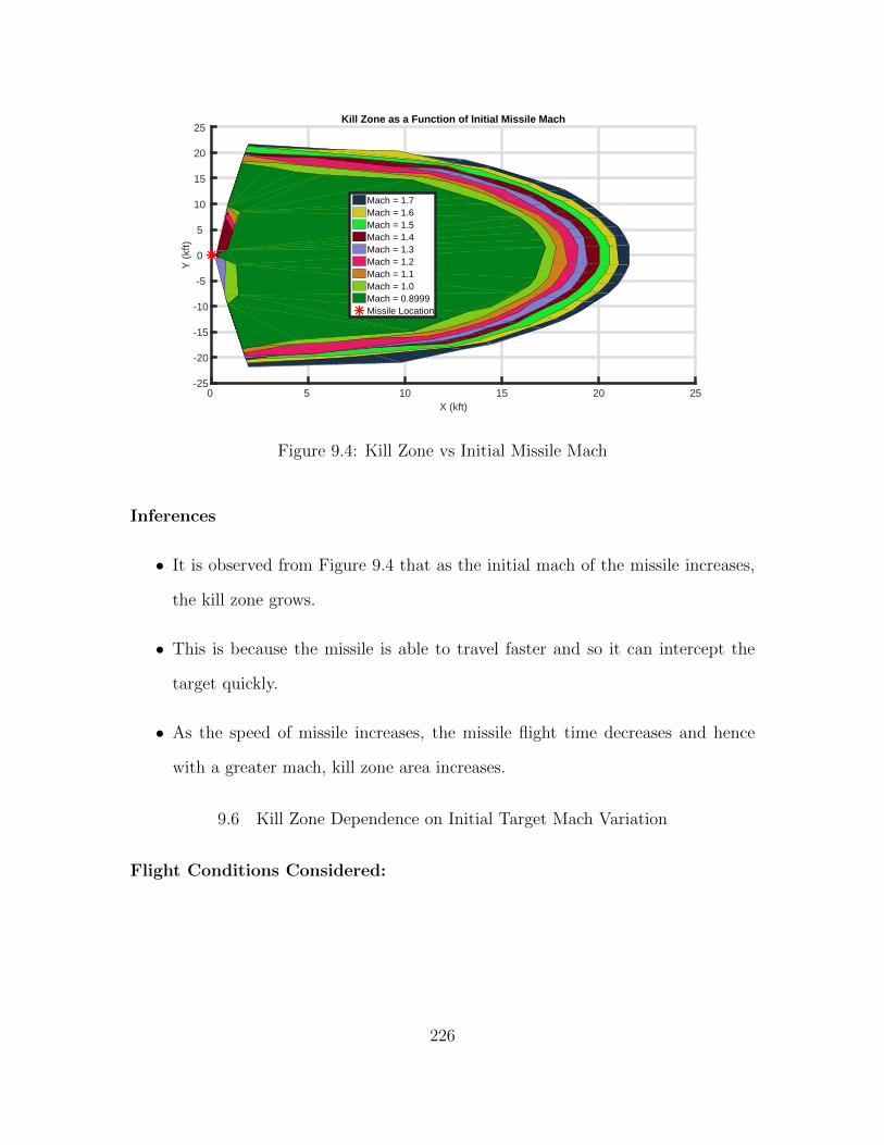
The results show what is expected. The kill zone increases with larger initial missile
Mach and maximum acceleration & decreases with higher engagement altitude and
higher target Mach. The environment is based on (1) a 6DOF bank-to-turn (BTT)
missile, (2) a full aerodynamic-stability derivative look up tables ranging over Mach
number, angle of attack and sideslip angle (3) a standard atmosphere model, (4) actu-
ator dynamics for each of the four cruciform fins, (5) seeker dynamics, (6) a nonlinear
autopilot, (7) a guidance system with three guidance algorithms (i.e. PNG, optimal,
differential game theory), (8) a 3DOF target model with three maneuverability mod-
els (i.e. constant speed, Shelton Turn & Climb, Riggs-Vergaz Turn & Dive). Each
of the subsystems are described within the research. The environment contains lin-
earization, model analysis and control design features. A gain scheduled nonlinear
BTT missile autopilot is presented here. Autopilot got sluggish as missile altitude
increased and got aggressive as missile mach increased. In short, the environment is
shown to be a very powerful tool for conducting missile-target engagement research -
a research that could address multiple missiles and advanced targets.
i
Dedicated to my parents and the loving memory of my brother Ravi
ii
ACKNOWLEDGMENTS
I want to thank the almighty for his blessings. First, I would like to express my
sincere gratitude to my MS thesis advisor Dr. Armando A. Rodriguez for showing
confidence in my work, his continuous motivation and support for my research, for
his patience, motivation, enthusiasm, and immense knowledge. His guidance helped
me throughout the course of the research and writing of this thesis. I could not have
imagined having a better advisor and mentor for my Masters studies. Besides my
thesis advisor, I would like to extend my gratitude to the rest of my thesis committee
Dr. Spring Berman and Dr. Panagiotis Artemiadis. I am grateful to all of the faculty
members who handled graduate courses for me at ASU.
I would also like to acknowledge the support of my fellow research mates Jesus
Aldaco Lopez(Thanks for those daily yoghurts & discussions), Zhichao Li, Xianglong
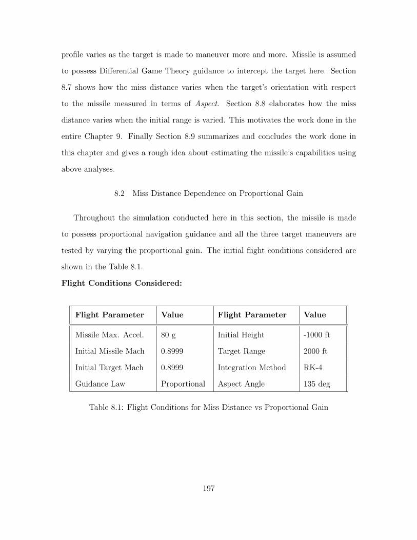
Table 8.1: Flight Conditions for Miss Distance vs Proportional Gain
197
−1 0 1 2 3 4 5 6 7 8 90
50
100
150
200
250
300
350
400
450
500
Proportional Navigation Gain
Mis
s D
ista
nce
(ft)
Miss Distance vs Proportional Navigation Gain
No AccelerationSheldon Turn & ClimbRiggs Vergaz Turn & Dive
Figure 8.1: Miss Distance vs Proportional Gain
2 3 4 5 6 7 80
5
10
15
20
25
30
35
40
45
Proportional Navigation Gain
Mis
s D
ista
nce
(ft)
Miss Distance vs Proportional Navigation Gain
No AccelerationSheldon Turn & ClimbRiggs Vergaz Turn & Dive
Figure 8.2: Zoomed in Figure 8.1
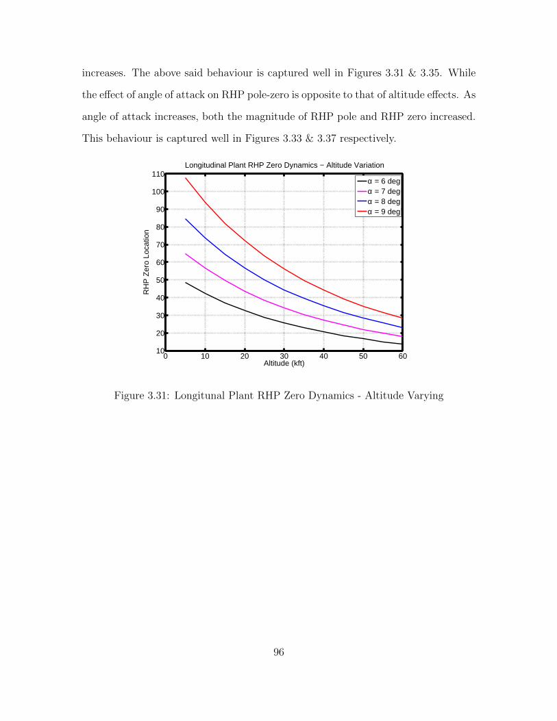
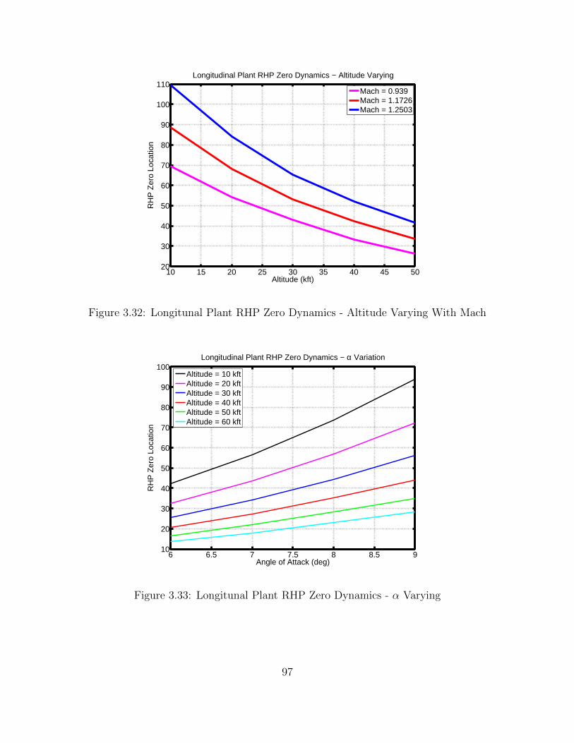
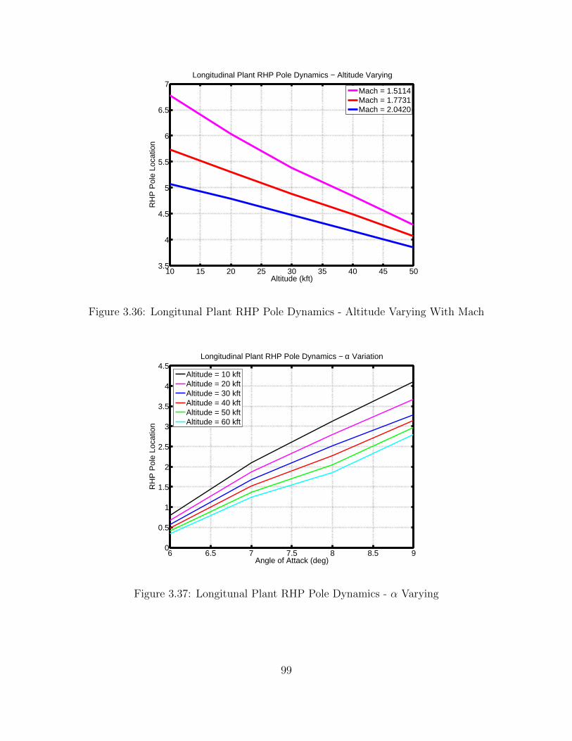
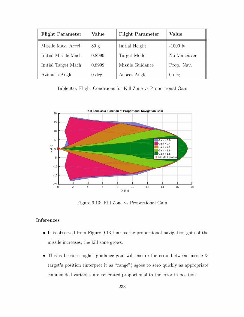
Inferences.
• From Figures 8.1 and 8.2, it is clearly evident that the miss distance is higher
198
when the proportional gain is too small and the miss distance reaches the min-
imum value which is unique for different flight conditions.
• Beyond the minimum, the miss distance increases slowly as we increase the gain
and this behaviour persists irrespective of the target maneuver.
• It is intuitive that if the proportional gain is very small, the missile will respond
slowly and will not be able to catch the target and similarly if the gain is big,
the outer guidance loop will become unstable due to the high frequency seeker
dynamics.
• It is also observed that these changes are observed only when the initial altitude
is small. At higher altitudes, the miss distance essentially becomes independent
of the gain.
• The reader is referred to the [17] for further insight and information about this
section.
8.3 Miss Distance Dependence on Initial Engagement Altitude
Throughout the simulation conducted here in this section, the missile is made
to possess different guidance laws and all the three target maneuvers are tested by
varying the initial engagement altitude. The initial flight conditions considered are
shown in the Table 8.2.
Flight Conditions Considered:
199
Flight Parameter Value Flight Parameter Value
Missile Max. Accel. 80 g Maneuver Index 0.25
Initial Missile Mach 0.8999 Target Range 2000 ft
Initial Target Mach 0.8999 Intgration Method RK-4
Proportional Gain 2.1 Aspect Angle 135 deg
Table 8.2: Flight Conditions for Miss Distance vs Engagement Altitude
0 10 20 30 40 50 60 70 800
50
100
150
200
250
300
350
400
450
500
Altitude (kft)
Mis
s D
ista
nce
(ft)
Miss Distance vs Altitude (No Maneuver)
Proportional NavigationOptimal TheoryDifferential Game Theory
Figure 8.3: Miss Distance vs Engagement Altitude - No Maneuver
200
0 10 20 30 40 50 60 70 800
50
100
150
200
250
300
350
400
450
500
Altitude (kft)
Mis
s D
ista
nce
(ft)
Miss Distance vs Altitude (Sheldon Maneuver)
Proportional NavigationOptimal TheoryDifferential Game Theory
Figure 8.4: Miss Distance vs Engagement Altitude - Sheldon Maneuver
0 10 20 30 40 50 60 70 800
50
100
150
200
250
300
350
400
450
500
Altitude (kft)
Mis
s D
ista
nce
(ft)
Miss Distance vs Altitude (Riggs Vergaz Maneuver)
Proportional NavigationOptimal TheoryDifferential Game Theory
Figure 8.5: Miss Distance vs Engagement Altitude - Riggs Vergaz Maneuver
201
0 10 20 30 40 50 60 70 800
50
100
150
200
250
300
350
400
450
500
Altitude (kft)
Mis
s D
ista
nce
(ft)
Miss Distance vs Altitude
Prop. Nav. − No ManeuverOpt. Th. − No ManeuverDiff Game − No ManeuverProp. Nav. − Sheldon ManeuverOpt. Th. − Sheldon ManeuverDiff Game − Sheldon ManeuverProp. Nav. − Riggs Vergaz ManeuverOpt. Th. − Riggs Vergaz ManeuverDiff Game − Riggs Vergaz Maneuver
Figure 8.6: Miss Distance vs Engagement Altitude - All Maneuvers
Inferences.
• As Altitude increases, the miss distance increases.
• It is intuitive that the air density decreases with increasing altitude, one might
expect that the missile fins lose their aerodynamic effectiveness at higher alti-
tudes.
• Figures 8.3 - 8.6 supports our intuitive inference about the inability of the fins
to control the missile in the thin air of the upper atmosphere.
• The reader is referred to the [17] for further insight and information about this
section.
8.4 Miss Distance Dependence on Missile Maximum Acceleration
Throughout the simulation conducted here in this section, the missile is made to
possess different guidance laws and all the three target maneuvers are tested by vary-
202
ing the initial maximum missile acceleration. The initial flight conditions considered
are shown in the Table 8.3.
Flight Conditions Considered:
Flight Parameter Value Flight Parameter Value
Proportional Gain 2.1 Maneuver Index 0.25
Initial Missile Mach 0.8999 Target Range 2000 ft
Initial Target Mach 0.8999 Time Constant 0.5 sec
Altitude -1000 ft Aspect Angle 135 deg
Table 8.3: Flight Conditions for Miss Distance vs Missile Maximum Acceleration
10 20 30 40 50 60 70 800
100
200
300
400
500
600
Missile Maximum Acceleration (g)
Mis
s D
ista
nce
(ft)
Miss Distance vs Missile Maximum Acceleration (No Maneuver)
Proportional NavigationOptimal Control TheoryDifferential Game Theory
Figure 8.7: Miss Distance vs Missile Max. Acceleration - No Maneuver
203
50 55 60 65 70 75 80
0
10
20
30
40
50
60
70
80
Missile Maximum Acceleration (g)
Mis
s D
ista
nce
(ft)
Miss Distance vs Missile Maximum Acceleration (No Maneuver)
Proportional NavigationOptimal Control TheoryDifferential Game Theory
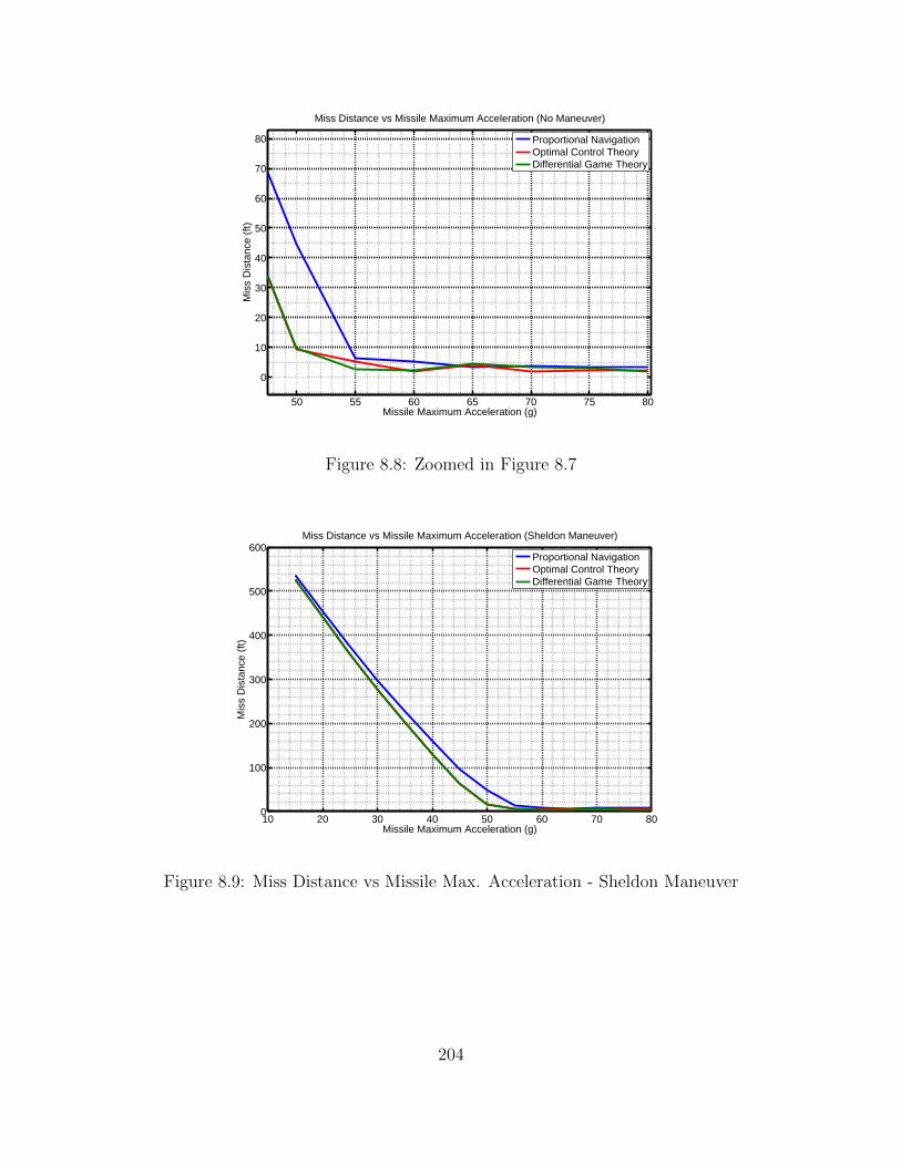
Figure 8.8: Zoomed in Figure 8.7
10 20 30 40 50 60 70 800
100
200
300
400
500
600
Missile Maximum Acceleration (g)
Mis
s D
ista
nce
(ft)
Miss Distance vs Missile Maximum Acceleration (Sheldon Maneuver)
Proportional NavigationOptimal Control TheoryDifferential Game Theory
Figure 8.9: Miss Distance vs Missile Max. Acceleration - Sheldon Maneuver
204
50 55 60 65 70 75 800
10
20
30
40
50
60
70
80
Missile Maximum Acceleration (g)
Mis
s D
ista
nce
(ft)
Miss Distance vs Missile Maximum Acceleration (Sheldon Maneuver)
Proportional NavigationOptimal Control TheoryDifferential Game Theory
Figure 8.10: Zoomed in Figure 8.9
10 20 30 40 50 60 70 800
100
200
300
400
500
600
Missile Maximum Acceleration (g)
Mis
s D
ista
nce
(ft)
Miss Distance vs Missile Maximum Acceleration (Riggs Vergaz Maneuver)
Proportional NavigationOptimal Control TheoryDifferential Game Theory
Figure 8.11: Miss Distance vs Missile Max. Acceleration - Riggs Vergaz Maneuver
205
50 55 60 65 70 75 800
10
20
30
40
50
60
70
80
Missile Maximum Acceleration (g)
Mis
s D
ista
nce
(ft)
Miss Distance vs Missile Maximum Acceleration (Riggs Vergaz Maneuver)
Proportional NavigationOptimal Control TheoryDifferential Game Theory
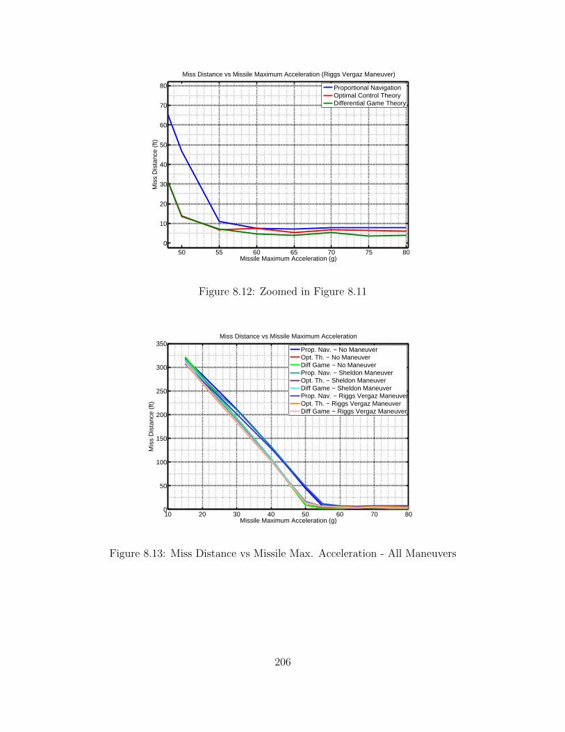
Figure 8.12: Zoomed in Figure 8.11
10 20 30 40 50 60 70 800
50
100
150
200
250
300
350
Missile Maximum Acceleration (g)
Mis
s D
ista
nce
(ft)
Miss Distance vs Missile Maximum Acceleration
Prop. Nav. − No ManeuverOpt. Th. − No ManeuverDiff Game − No ManeuverProp. Nav. − Sheldon ManeuverOpt. Th. − Sheldon ManeuverDiff Game − Sheldon ManeuverProp. Nav. − Riggs Vergaz ManeuverOpt. Th. − Riggs Vergaz ManeuverDiff Game − Riggs Vergaz Maneuver
Figure 8.13: Miss Distance vs Missile Max. Acceleration - All Maneuvers
206
50 55 60 65 70 75 800
10
20
30
40
50
60
Missile Maximum Acceleration (g)
Mis
s D
ista
nce
(ft)
Miss Distance vs Missile Maximum Acceleration
Prop. Nav. − No ManeuverOpt. Th. − No ManeuverDiff Game − No ManeuverProp. Nav. − Sheldon ManeuverOpt. Th. − Sheldon ManeuverDiff Game − Sheldon ManeuverProp. Nav. − Riggs Vergaz ManeuverOpt. Th. − Riggs Vergaz ManeuverDiff Game − Riggs Vergaz Maneuver
Figure 8.14: Zoomed in Figure 8.13
Inferences.
• As missile maximum acceleration increases, the miss distance decreases.
• This goes well with our intuition that given an higher acceleration advantage for
the missile over the target, it is easier for the missile to track down the target.
• Figures 8.7 - 8.14 support our inferences.
• It is also seen that irrespective of the different target maneuver and different
missile guidance laws, the above said conjecture seems to hold true.
8.5 Miss Distance Dependence on Initial Missile Mach
Throughout the simulation conducted here in this section, the missile is made to
possess proportional guidance law and the target has no maneuver and this scenario
is tested by varying the initial missile Mach. The initial flight conditions considered
are shown in the Table 8.4.
207
Flight Conditions Considered:
Flight Parameter Value Flight Parameter Value
Missile Max. Accel. 80 g Initial Height -1000 ft
Integration Method RK-4 Target Range 10000 ft
Initial Target Mach 0.8999 Time Constant 0.5 sec
Target Mode Const. Ve-
locity
Aspect Angle 135 deg
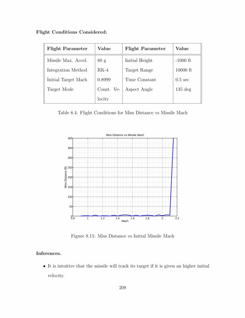
Table 8.4: Flight Conditions for Miss Distance vs Missile Mach
0.8 1 1.2 1.4 1.6 1.8 2 2.20
50
100
150
200
250
300
350
400
Mach
Mis
s D
ista
nce
(ft)
Miss Distance vs Missile Mach
Figure 8.15: Miss Distance vs Initial Missile Mach
Inferences.
• It is intuitive that the missile will track its target if it is given an higher initial
velocity.
208
• But it is also a point of interest to note here that, if the missile initial velocity
is very big, e.g. here in our case if it is bigger than 2.15 for the above flight
condition considered, the missile permanenetly misses the target because it had
travelled probably in the wrong direction initially with higher velocity.
• Missile realizes that the it cannot track down its target as the range keeps on
increasing.
• That is not captured here in Figure 8.15 as miss distance is a very big number
in those cases.
• This scenario can be thought analogous to a condition where our integration
step size is big.
• Reader is referred to the Section 7.3 in Chapter 7.
8.6 Miss Distance Dependence on Target Maneuver
Throughout the simulation conducted here in this section, the missile is made
to possess differential game theory guidance and all the three target maneuvers are
tested by varying the proportional gain. The initial flight conditions considered are
shown in the Table 8.5.
Flight Conditions Considered:
209
Flight Parameter Value Flight Parameter Value
Missile Max. Accel. 80 g Initial Height -1000 ft
Initial Missile Mach 0.8999 Target Range 2000 ft
Initial Target Mach 0.8999 Time Constant 0.5 sec
Integration Method RK-4 Aspect Angle 135 deg
Table 8.5: Flight Conditions for Miss Distance vs Target Maneuver
0 0.5 1 1.5 2 2.5 3 3.50
50
100
150
200
250
300
350
Target Maneuver Index
Mis
s D
ista
nce
(ft)
Miss Distance vs Target Maneuver Index
No AccelerationSheldon Turn & ClimbRiggs Vergaz Turn & Dive
Figure 8.16: Miss Distance vs Target Maneuver
210
0.1 0.2 0.3 0.4 0.5 0.6 0.7 0.8 0.9
0
5
10
15
20
Target Maneuver Index
Mis
s D
ista
nce
(ft)
Miss Distance vs Target Maneuver Index
No AccelerationSheldon Turn & ClimbRiggs Vergaz Turn & Dive
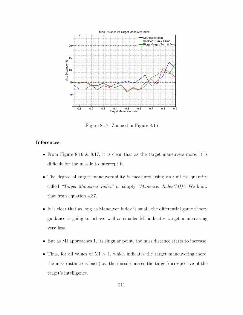
Figure 8.17: Zoomed in Figure 8.16
Inferences.
• From Figure 8.16 & 8.17, it is clear that as the target maneuvers more, it is
difficult for the missile to intercept it.
• The degree of target maneuverability is measured using an unitless quantity
called “Target Maneuver Index” or simply “Maneuver Index(MI)”. We know
that from equation 4.37.
• It is clear that as long as Maneuver Index is small, the differential game thoery
guidance is going to behave well as smaller MI indicates target maneuvering
very less.
• But as MI approaches 1, its singular point, the miss distance starts to increase.
• Thus, for all values of MI > 1, which indicates the target maneuvering more,
the miss distance is bad (i.e. the missile misses the target) irrespective of the
target’s intelligence.
211
• This behaviour is excellently captured in the Figure 8.16.
• For more information on this concept, the reader is referred to the relevant GNC
texts [51] and [52].
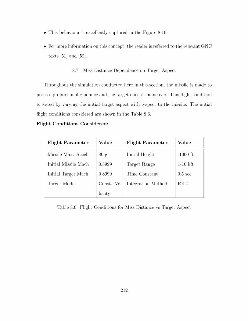
8.7 Miss Distance Dependence on Target Aspect
Throughout the simulation conducted here in this section, the missile is made to
possess proportional guidance and the target doesn’t maneuver. This flight condition
is tested by varying the initial target aspect with respect to the missile. The initial
flight conditions considered are shown in the Table 8.6.
Flight Conditions Considered:
Flight Parameter Value Flight Parameter Value
Missile Max. Accel. 80 g Initial Height -1000 ft
Initial Missile Mach 0.8999 Target Range 1-10 kft
Initial Target Mach 0.8999 Time Constant 0.5 sec
Target Mode Const. Ve-
locity
Integration Method RK-4
Table 8.6: Flight Conditions for Miss Distance vs Target Aspect
212
0 20 40 60 80 100 120 140 160 1800
500
1000
1500
2000
2500
3000
3500
4000
4500
Aspect Angle (deg)
Mis
s D
ista
nce
(ft)
Miss Distance vs Aspect Angle
Range = 1000 ftRange = 2000 ft
Figure 8.18: Miss Distance vs Target Aspect - Range = 1 kft, 2 kft
20 40 60 80 100 120
−5
0
5
10
Aspect Angle (deg)
Mis
s D
ista
nce
(ft)
Miss Distance vs Aspect Angle
Range = 1000 ftRange = 2000 ft
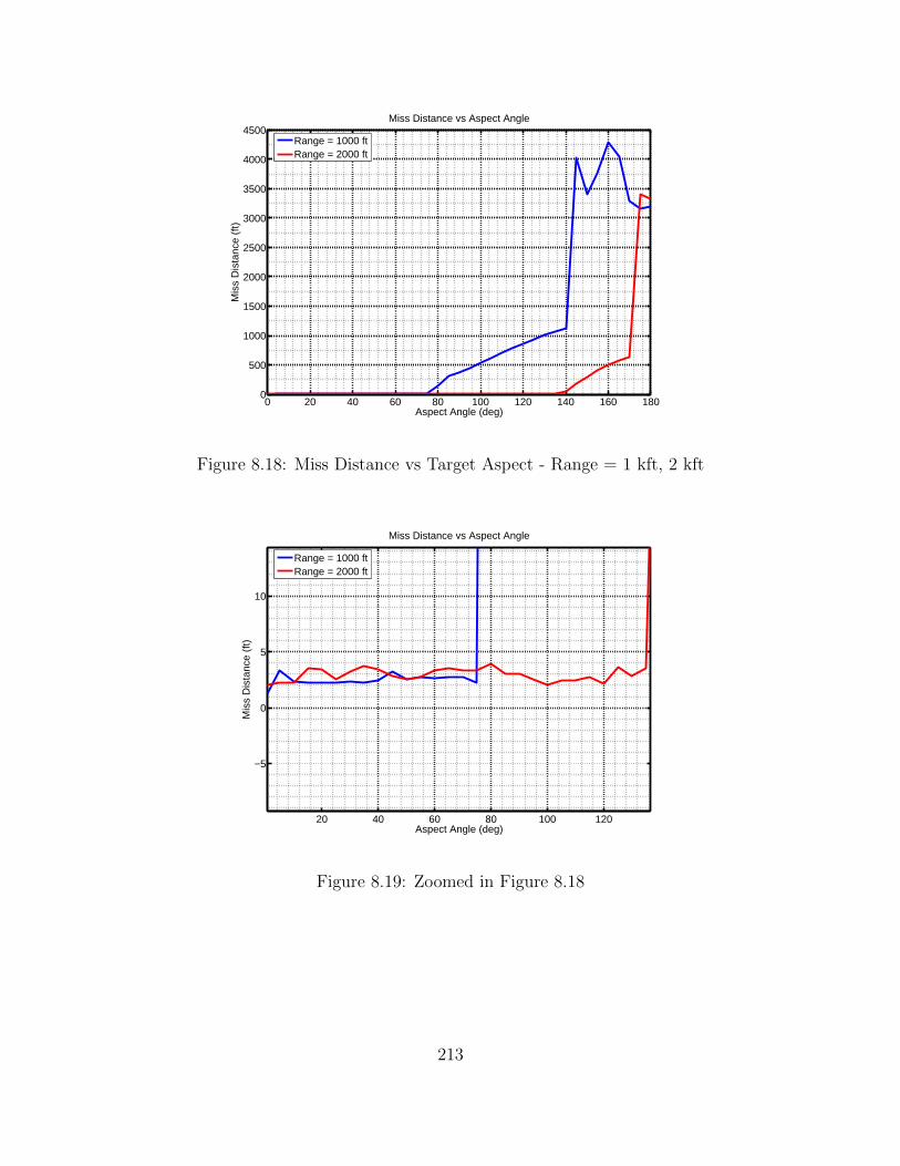
Figure 8.19: Zoomed in Figure 8.18
213
0 20 40 60 80 100 120 140 160 1800
2
4
6
8
10
12
14
Aspect Angle (deg)
Mis
s D
ista
nce
(ft)
Miss Distance vs Aspect Angle
Range = 3000 ftRange = 4000 ftRange = 6000 ftRange = 8000 ftRange = 10000 ft
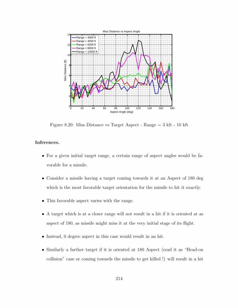
Figure 8.20: Miss Distance vs Target Aspect - Range = 3 kft - 10 kft
Inferences.
• For a given initial target range, a certain range of aspect angles would be fa-
vorable for a missile.
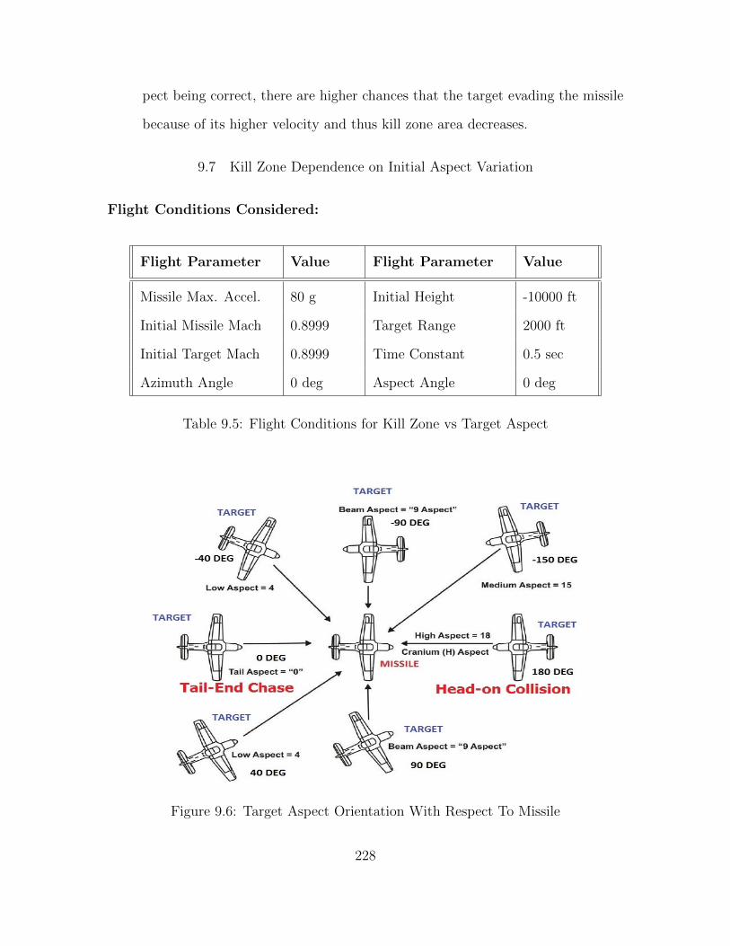
• Consider a missile having a target coming towards it at an Aspect of 180 deg
which is the most favorable target orientation for the missile to hit it exactly.
• This favorable aspect varies with the range.
• A target which is at a closer range will not result in a hit if it is oriented at as
aspect of 180, as missile might miss it at the very initial stage of its flight.
• Instead, 0 degree aspect in this case would result in an hit.
• Similarly a farther target if it is oriented at 180 Aspect (read it as “Head-on
collision” case or coming towards the missile to get killed !) will result in a hit
214
condition, while 0 deg aspect would clearly result in an miss since missile is not
guaranteed to succeed in a tail end chase with target being very far.
• This phenomenon is clearly captured in Figures 8.18 - 8.20.
• As we increase the range, all aspect angles from 0 to 180 degree is expected to
give an hit.
• But going by the basic Physics, if we go on increase the range, there will be a
point where missile will start to miss the target.
• This is explained in below Section 8.8 and this also motivates the work done in
the Chapter 9.
• Thus Aspect is a very important parameter in missile-target engagement and it
depends upon initial target range.
8.8 Miss Distance Dependence on Initial Target Range
Throughout the simulation conducted here in this section, the missile is made
to possess proportional guidance with proportional navigation gain of about 2.3 for
both the channels and the target doesn’t maneuver. This flight condition is tested by
varying the initial target range with respect to the missile. The initial flight conditions
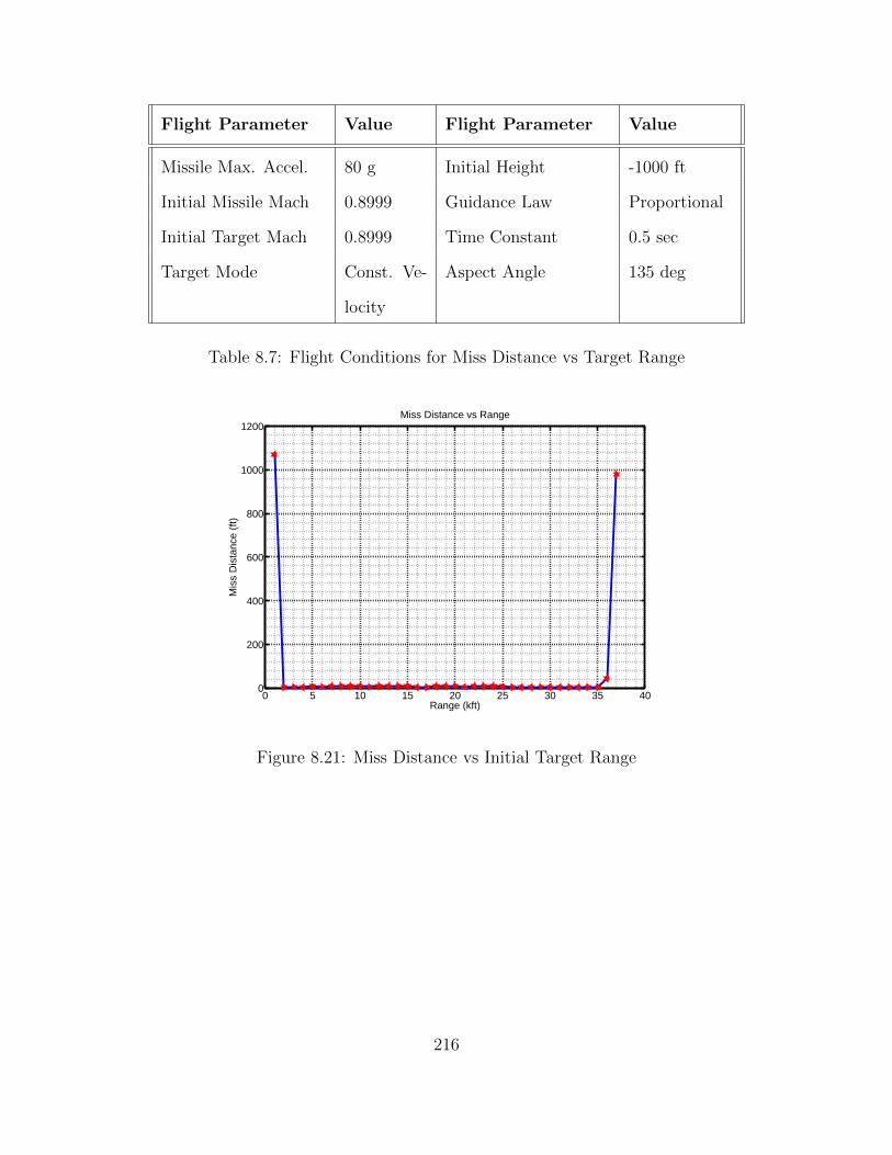
considered are shown in the Table 8.7. Aspect of 135 degrees is considered here.
Flight Conditions Considered:
215
Flight Parameter Value Flight Parameter Value
Missile Max. Accel. 80 g Initial Height -1000 ft
Initial Missile Mach 0.8999 Guidance Law Proportional
Initial Target Mach 0.8999 Time Constant 0.5 sec
Target Mode Const. Ve-
locity
Aspect Angle 135 deg
Table 8.7: Flight Conditions for Miss Distance vs Target Range
0 5 10 15 20 25 30 35 400
200
400
600
800
1000
1200
Range (kft)
Mis
s D
ista
nce
(ft)
Miss Distance vs Range
Figure 8.21: Miss Distance vs Initial Target Range
216
5 10 15 20 25 30 350
10
20
30
40
50
60
70
80
Range (kft)
Mis
s D
ista
nce
(ft)
Miss Distance vs Range
Figure 8.22: Zoomed in Figure 8.21
Inferences.
• For the given aspect, from Figures 8.21 & 8.22 reveal that smaller ranges end
up with high miss distance as missile might initially move in wrong direction
and miss the target completely.
• As range increases, missile can catch up with target’s range and its orientation
and thus our miss distance in those range is very small.
• Finally as the target is far away, missile will start to run out of fuel while
catching up with the target and misses it.
• This clearly motivates the kill estimation work done in Chapter 9.
• Referring to the previous Section 8.7, for different target aspect, the hitting
ranges including from closest hit till the farthest hit will vary.
217
8.9 Summary and Conclusions
In this chapter, the miss distance profiles with respect to different missile/target
engagement parameters were discussed. This will give us a fair idea about how the
miss distance varies as we vary different missile-target engagement parameters. This
shall definitely help us in estimating the capability of a BTT missile.
218
Chapter 9
KILL ZONE COMPUTATION & ANALYSIS
9.1 Introduction and Overview
Launching missiles effectively with high success rate is a complex resource alloca-
tion problem. The cost of manufacturing and operating each missile is realtively very
high and so they have to be launched only when their success is guaranteed. If the
hunting area of the missile with its full capability is known, then any target spotted
within the hunting area can be successfully intercepted by launching the missile. The
purpose of this chapter is to illustrate the hunting zone of the BTT missile considered
in this research. Given a thrust profile and fixed initial conditions for both missile and
target, the analysis made in this chapter will explain about the zone of kill where the
missile will successfully intercept the target. Kill Zone is a closed area on the space
which includes all possible target’s starting position, which will result in the missile
intercepting the target. Estimating such a big area in 2D space will need a powerful
estimation algorithm for faster computation and binary search algorithm [71] & [72]
is used here. The research here has been restricted to 2D space by assuming both the
missile and target initially start at the same altitude with respect to each other. The
high fidelity environment used throughout the simulation in this research is employed
to study the Kill Zone profile with respect to different missile/target engagement pa-
rameters using ideas described in the relevant GNC textbooks [51] and [52]. Also the
work done in this chapter takes its motivation from the Section 8.8 in the Chapter 8.
Conventional warheads carried by the missile have a circular blast radius of about
219
20 ft [70]. Thus any simulation resulting in a final miss distance less than 20 feet is
taken granted as a hit and kill zone estimation is developed as per this logic. Each
section in this chapter will have information about the flight conditions considered, the
result and its inference. The chapter is organized as follows: Section 9.2 will give an
brief overview about the binary search algorithm and its usage here in our simulation.
Section 9.3 analyses the effect of altitude variation on the estimated kill zone. Section
9.4 throws light on effect of varying the maximum acceleration capability of the missile
over on the estimated kill zone. Section 9.5 discusses the effect of initial missile speed
on the estimated kill zone. Section 9.6 discusses the effect of initial target speed on
the estimated kill zone. Section 9.7 shows how the estimated kill zone varies when the
target’s orientation with respect to the missile measured in terms of Aspect. Section
9.8 will briefly discuss the estimated kill zone change when the proportional gain is
varied. Here the missile is assumed to possess Proportional Navigation guidance law
to intercept the target. Finally Section 9.9 summarizes and concludes the work done
in this chapter and gives a rough idea about estimating the missile’s area of kill using
above analyses.
9.2 Binary Search Algorithm
When we have an infinite 2D space, it is very important to chose a proper algo-
rithm for finding out the kill zone area in a shorter span of time. Naturally binary
search will eliminate half of the unwanted space in each and every iteration and help
us to converge faster towards the solution. As per the current simulation used here,
the time required to obtain a kill zone for one flight condition is approximately 1
minute. For knowing more about the binary search algorithm, the reader is referred
to [22], [71] and [72]. Since we are assuming both the missile and target to start
at the same altitude, the search space reduces to 2D. Now the 2D space is divided
220
radially into 360 rays. The challenge here was to find the first hit point and last hit
point along each ray. The following algorithm was used.
Algorithm Steps.
1. Initially the algorithm is started by placing the target to be 100 ft away from
missile along the 180 degree ray.
2. It is assumed that below range of 100 ft, it is pointless to launch a missile
against a target.
3. Now if it is a hit, we double the range and search for a miss or if it is a miss,
we take the average between current hit range and miss range.
4. Thus along a ray, we would find the first hit position.
5. Then the algorithm is restarted with twice the current hit range looking for
final hit range.
6. After averaging and converging to an hit range which differs from miss range
by just 100 ft, we stop the algorithm.
7. This idea is repeated for all the rays. Each ray can be incremented in steps of
2 or 5 degrees to suit the degree of accuracy needed.
8. To speed up the operation, the previous ray final hit range is used in the current
ray final hit range estimation using the motivation from the continuity idea.
9. Finally only the hit positions data are stored. While post processing the data,
we prepare an array of initial hit positions and final hit positions along each ray
and finally plot them using the “boundary” command in MATLAB.
10. The above process is repeated by varying one of the flight condition parameter
and the estimated kill zone is plotted for that parameter variation.
221
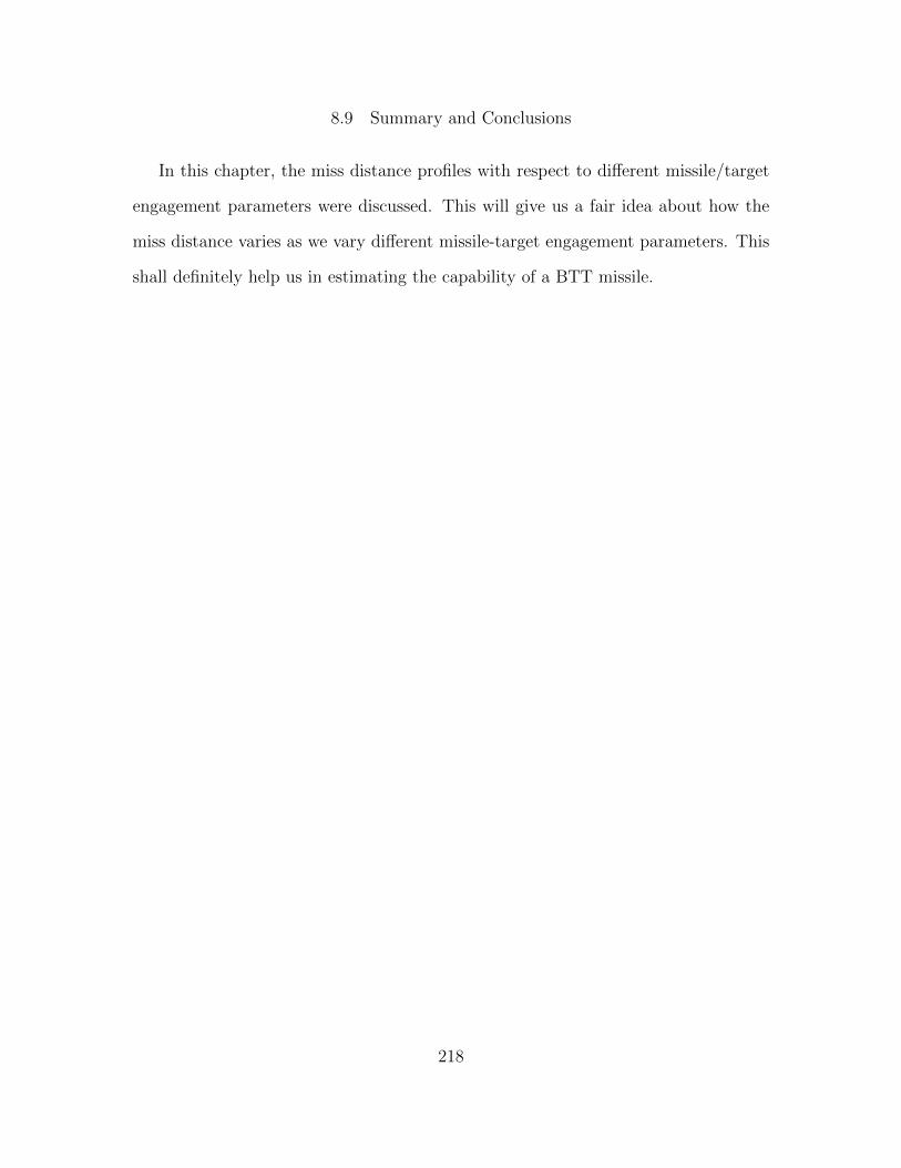
9.3 Kill Zone Dependence on Initial Engagement Altitude Variation
Flight Conditions Considered:
Flight Parameter Value Flight Parameter Value
Missile Max. Accel. 80 g Initial Height -10000 ft
Initial Missile Mach 0.8999 Target Range 2000 ft
Initial Target Mach 0.8999 Time Constant 0.5 sec
Azimuth Angle 0 deg Aspect Angle 0 deg
Table 9.1: Flight Conditions for Kill Zone vs Engagement Altitude
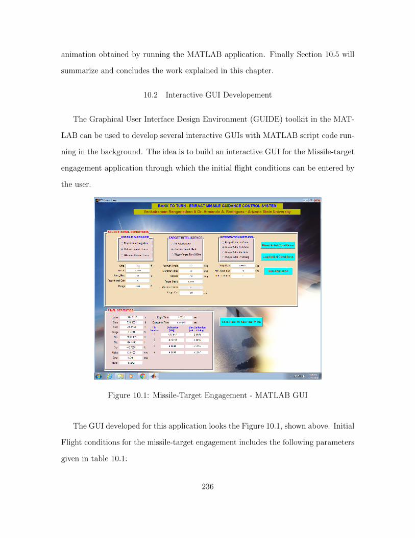
The GUI developed for this application looks the Figure 10.1, shown above. Initial
Flight conditions for the missile-target engagement includes the following parameters
given in table 10.1:
236
Missile Guidance Aspect Integration Method Range
Missile Max. Accel. Step Size Proportional Gain Maneuver Index
Target Mach Elevation Target Maneuver Azimuth
Target Altitude Missile Mach Missile Altitude Target Tau
Table 10.1: GUI Flight Conditions Selection for Missile-Target Engagement
• Once the above parameters are selected, the Load Initial Conditions button is
hit.
• Internally MATLAB will create Missile & Target Class objects and loads the
user entered initial flight conditions.
• Then the Run Animation button is hit which will start the Missile-Target En-
gagement simulation and each and every step of the simulation is updated using
an 3D animation which was developed using VRML toolbox in MATLAB.
• Once the animation, i.e., the simuation gets over, final statistics are displayed
and the post flight data can be analyzed by clicking Plot Data button.
• Thus in one single GUI screen, the user will be able to enter their desired initial
flight conditions, see the animation to get a virtual feel of how the missile would
intercept the target in real time and conclude by seeing all the final statistics
and the post flight data in the same screen.
10.3 3D Animation using MATLAB VRML Toolbox
VRML (Virtual Reality Modeling Language) toolbox in MATLAB can be used
to make different interactive animations. Here in this research, missile-target en-
gagement can be visualized using the features offered by the MATLAB. Since the
237
entire MATLAB application has been coded in an object oriented architecture, the
same program can be easily extended to multiple missile-target engagement just by
using new object for Missile and Target class. Thus the entire simulation data has
to be communicated to animating world in a way that it understands. Once that is
achieved, then whatever happens in simulation can be seen in real time 3D animation
as animation is just updating the simulation flow. The motivation for going for a 3D
animation is to visualize how the missile-target engagement would happen in a real
world scenario (which would be difficult for us to see in real time). And given a better
modeling and design environment, it can be believed that real missile would exactly
behave and intercept the target like it does in 3D animation. Several aerospace com-
panies spend billions of dollar in modeling the environment so that things if they
work in simulation well are expected to work almost the same way in real world.
Thus to prepare an interative 3D animation we require the following,
1. Nice and fancy 3D Background
2. Missile Object
3. Aircraft Object
4. Different Viewpoints
5. Proper interface between VRML editor and MATLAB - Could be either
through MATLAB or SIMULINK. MATLAB interface is used in this
research.
238
Figure 10.2: Missile-Target Engagement - 3D Animation
Figure 10.3: Missile-Target Engagement - 3D Animation Top View
3D World Editor - VRML Editor which comes as a part of MATLAB VRML tool-
box was used to develop the 3D animation environment. There are other commercial
VRML editors available in the market for cheaper costs like V-Realm Builder, 3DStu-
dio, Blender etc... 3D World Editor was good enough to prepare the animation in this
research. VRML files have “.wrl” format which is a short form for “world”. Initially
239
the 3D background was developed, then the missile and target objects were properly
placed in the 3D background in such a way as to mimick the initial conditions given
through the interactive MATLAB GUI. The VRML toolbox in MATLAB already
has different aerospace objects like aircraft, missile, helicopters, rockets etc. One
such missile and target aircraft from that repository is being used in this research.
Then the different viewpoints can be made according to the user requirements. A
missile cockpit viewpoint along with other 4 viewpoints were developed for this re-
search. For example, refer figure 10.3 for a top viewpoint. Cockpit viewpoint as
shown in Figure 10.2 will give a real-time feel as if we were sitting inside the missile
and riding it(Although never done in real life!). Different flight parameters of both
missile and target can be tracked as the animation progresses. This gives a real-time
feel like traveling in a fighter aircraft being a pilot. Given the power of GPUs nowa-
days, this missile-target engagement simulation can be made much faster, while the
current research is done without the usage of GPUs. Also, if the MATLAB is made
aware of intelligently using the GPUs, then this research can get really interesting.
There are other better softwares like Blender, Maya, 3DS Max which is capable of
creating content rich 3D object files in different format. As of now, good resource
files in “.wrl” format are really less available. MATLAB recently extended the 3D
animation capability to “.x3d” format too. Similarly there are ways to import 3D
object files from the 3D authoring worlds like AutoCAD, CATIA, Solidworks and so
into the MATLAB and create animations with them.
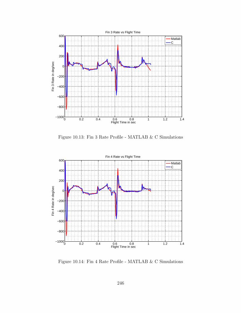
10.4 Simulation Results & Analysis
Post flight analysis from simulating the conditions from table 10.2 are plotted
and comparison of MATLAB results with C program [5] is presented. The plots
ranging from Figure 10.4 - 10.14 show that both C and MATLAB simulations are
240
really close to each other, depicting that MATLAB program is as accurate as C
program, eventhough it is written with different programming style and interpolating
techniques for calculating aerodynamic coefficients.
Flight Conditions Considered:
Flight Parameter Value Flight Parameter Value
Missile Max. Accel. 80 g Initial Height -1000 ft
Initial Missile Mach 0.8999 Target Range 2000 ft
Initial Target Mach 0.8999 Missile Guidance Optimal Control
Target Maneuver Sheldon Aspect Angle 0 deg
Table 10.2: Flight Conditions for MATLAB & C Simulations
0 0.2 0.4 0.6 0.8 1 1.2 1.40
5
10
15
20
25
30Alpha vs Flight Time
Flight Time in sec
Ang
le O
f Atta
ck in
deg
MatlabC
Figure 10.4: Alpha Profile - MATLAB & C Simulations
241
0 0.2 0.4 0.6 0.8 1 1.2 1.40
0.5
1
1.5
2
2.5
3
3.5Beta vs Flight Time
Flight Time in sec
Sid
eslip
Ang
le in
deg
MatlabC
Figure 10.5: Profile - MATLAB & C Simulations
0 0.2 0.4 0.6 0.8 1 1.2 1.40
200
400
600
800
1000
1200
1400
1600
1800
2000Range vs Flight Time
Flight Time in sec
Ran
ge in
feet
MatlabC
Figure 10.6: Profile - MATLAB & C Simulations
242
0 0.2 0.4 0.6 0.8 1 1.2 1.4−10
−8
−6
−4
−2
0
2
4Fin 1 Deflection vs Flight Time
Flight Time in sec
Fin
1 D
efle
ctio
n in
deg
MatlabC
Figure 10.7: Fin 1 Profile - MATLAB & C Simulations
0 0.2 0.4 0.6 0.8 1 1.2 1.4−12
−10
−8
−6
−4
−2
0
2
4Fin 2 Deflection vs Flight Time
Flight Time in sec
Fin
2 D
efle
ctio
n in
deg
MatlabC
Figure 10.8: Fin 2 Profile - MATLAB & C Simulations
243
0 0.2 0.4 0.6 0.8 1 1.2 1.4−6
−4
−2
0
2
4
6
8
10Fin 3 Deflection vs Flight Time
Flight Time in sec
Fin
3 D
efle
ctio
n in
deg
MatlabC
Figure 10.9: Fin 3 Profile - MATLAB & C Simulations
0 0.2 0.4 0.6 0.8 1 1.2 1.4−8
−6
−4
−2
0
2
4
6Fin 4 Deflection vs Flight Time
Flight Time in sec
Fin
4 D
efle
ctio
n in
deg
MatlabC
Figure 10.10: Fin 4 Profile - MATLAB & C Simulations
244
0 0.2 0.4 0.6 0.8 1 1.2 1.4−1400
−1200
−1000
−800
−600
−400
−200
0
200
400
600Fin 1 Rate vs Flight Time
Flight Time in sec
Fin
1 R
ate
in d
eg/s
ec
MatlabC
Figure 10.11: Fin 1 Rate Profile - MATLAB & C Simulations
0 0.2 0.4 0.6 0.8 1 1.2 1.4−1400
−1200
−1000
−800
−600
−400
−200
0
200
400
600Fin 2 Rate vs Flight Time
Flight Time in sec
Fin
2 R
ate
in d
eg/s
ec
MatlabC
Figure 10.12: Fin 2 Rate Profile - MATLAB & C Simulations
245
0 0.2 0.4 0.6 0.8 1 1.2 1.4−1000
−800
−600
−400
−200
0
200
400
600Fin 3 Rate vs Flight Time
Flight Time in sec
Fin
3 R
ate
in d
eg/s
ec
MatlabC
Figure 10.13: Fin 3 Rate Profile - MATLAB & C Simulations
0 0.2 0.4 0.6 0.8 1 1.2 1.4−1000
−800
−600
−400
−200
0
200
400
600Fin 4 Rate vs Flight Time
Flight Time in sec
Fin
4 R
ate
in d
eg/s
ec
MatlabC
Figure 10.14: Fin 4 Rate Profile - MATLAB & C Simulations
246
10.5 Summary and Conclusions
In this chapter, developement of 3D animation using MATLAB VRML toolbox is
explained in detail. Also development of interactive GUI for entering the initial flight
conditions is explained. Visualization of missile-target engagement using MATLAB
will enable us to explore future research, behaviour of both missile and target can be
studied thoroughly. Finally the MATLAB simulation results are compared with C
program [5] results and accuracy of MATLAB simulation is ascertained.
247
Chapter 11
SUMMARY & DIRECTIONS FOR FUTURE RESEARCH
11.1 Summary of Work
This thesis addressed about the analysis, and control issues that are critical about
the BTT missiles. The following summarizes key themes within the thesis.
1. Literature Survey. A fairly comprehensive literature survey of relevant work
was presented.
2. Modeling. A nonlinear dynamical model for the BTT missile was presented
and linearization analysis was performed to understand the full utility of each
model.
3. Control. Both inner-loop and outer-loop control designs were discussed in
the context of an overall hierarchical control inner-outer loop framework. This
framework lends itself to accommodate multiple phase of missile flight; The
need for an nonlinear gain scheduled autopilot was explored and a sample non-
linear autopilot was obtained using incremental nonlinear dynamic inversion
technique for the innermost rate control loop design. Comprehensive inner-loop
trade studies were conducted for the BTT missile. A great deal of effort was
spent on discussion fundamental performance limitations. Attention was spent
on numerical integration step size limitations as well as dynamic (bandwidth)
limitations.
248
4. Miss Distance Analysis. Set of missile-target engagement simulations were
carried out by varying various missile flight conditions and their effects on final
miss distance was analyzed and tabulated.
5. Kill Zone Analysis. Using Binary Search algorithm, a closed area in 2D
space where the probability of missile hitting the target being high was esti-
mated. The estimated result is analyzed for various flight parameter variations
and tabulated.
6. Animation Demonstrations. Many animation demonstrations were con-
ducted - with animation corroborating the simulation data results.
11.2 Directions for Future Research
Complicated research topic like missile control always presents great deal of fu-
ture topics to explore. Remember uncertainity modeling in plant dynamics is not
addressed here. Things get interesting when we try to include uncertainity model in
our control design and we would like to see how they affect our robustness properties
at different loop breaking points. Thus looking forward from the research conducted
here, following points will throw some light on future topics to explore.
1. Integrated Guidance Navigation & Control (GNC) design where guidance loop
is designed as a part of autopilot and the new design can be studied for its
robustness.
2. Studying missile-target engagement with a 6DOF target and learn when would
we need such a complicated target over a simple 3DOF target which is used in
this research. Remember when target is 6DOF, it will have its own autopilot.
249
3. Trying out different target intelligence algorithms and learn how an increase in
target intelligence would affect the missile’s tracking ability.
4. Extending current 2D kill zone search to 3D search space, where both missile
and target can start at any altitude. Also analyzing the same 3D kill zone
with respect to different missile-target engagement parameters and comparitive
studies can be done with 2D kill zone results presented in this thesis.
5. Optimal Control missile guidance law suffers from poor Time-To-Go estimate
problem. This can be addressed using an Extended Kalman Filter (EKF) algo-
rithm.
6. Extending one-on-one missile target engagement to multiple missile-target en-
gagement. Multiple missiles can be made to chose their target dynamically on
the run-time based on some state of emergency (need of the hour) or lethal
nature of target. This is a very interesting resource allocation problem and
interessting solutions can be achieved using game theory techniques developed
for pursuit evasion problems.
250
REFERENCES
[1] Sonne M., Rodriguez A. A., “A Viable PC Tool for the Design and Evaluationof Missile Guidance and Control Systems,” Proceedings of the American ControlConference, Baltimore, MD, June 29-July 1, 1994, pp. 2726-2730.
[2] Wallis M., Feeley J., “BTT Missile-Target Simulations on a Desktop Computer,”The Soc. for Comp. Sim. Int., 1989, pp. 79-84.
[3] Riggs T., Vergaz B., “Adv. Air-to-Air Missile Gui. Using Opt. Control and Est,”AFATL-TR-81-56 AFAL, Eglin AFB, FL.
[4] Sheldon L. C., “6DOF BTT Missile Simulations of the ILAAT Missile with Lookuptables for the Aerodynamic Coefficients,” Air force Armament Laboratory, EglinAFB, FL, 1986.
[5] Sonne M. L., Use of PC’s in Evaluation and Design of Missile Guidance andControl Systems, Arizona State University, MS Thesis, 1994.
[6] Jenniges A., Simulink Based Evaluation and Design of Missile Guidance and Con-trol Systems, Arizona State University, Independent Study Report, 1998.
[7] Cimen T., “A Generic Approach to Missile Autopilot Design using State-Dependent Nonlinear Control,” Preprints of the 18th IFAC World Congress, Mi-lano, Italy, August 28 - September 2, 2011, pp. 9587 - 9600.
[8] Siddarth A. N., Peter F., Holzapfel F., Valasek J., “Autopilot for a NonlinearNon-Minimum Phase Tail-Controlled Missile,” AIAA Guidance, Navigation, andControl Conference, 13-17 January 2014, National Harbor, Maryland.
[9] Wang G., Mei W., Liu H., Xiao Y., “The Design of Virtual Reality Flight Simula-tion Platform Based on Rigid Body Kinematics,” International Journal of DigitalContent Technology and its Applications(JDCTA), Vol. 7, No. 7, April 2013.
[10] Cloutier J. R., Stansbery D. T., “Nonlinear, Hybrid Bank-to-Turn/Skid-to-TurnMissile Autopilot Design,” Proceedings of AIAA Guidance, Navigation & ControlConference, Montreal, Canada, August 2001.
[11] Cloutier J. R., “State-Dependent Riccati Equation Techniques: An Overview,”Proceeding of American Control Conference, Albuquerque, New Mexico, June1997.
[12] Hawley P. A., Blauwkamp R. A., “Six-Degree-of-Freedom Digital Simulations forMissile Guidance, Navigation and Control,” John Hopkins APL Technical Digest,Vol. 29, No. 1, 2010.
[13] Jackson P. B., “Overview of Missile Flight Control Systems,” John Hopkins APLTechnical Digest, Vol. 29, No. 1, 2010.
251
[14] Kaplan J. A., Chappell A. R., Mcmanus J. W., “The Analysis of a Generic Air-to-Air Missile Simulation Model,” NASA Technical Memorandum 109057, June1994.
[15] Rodriguez A. A., Sonne M., “The PC as a Viable Tool in the Design and Evalu-ation Process of Guidance and Control Systems for Missiles,” Proceedings of the1994 International Conference on Simulation in Engineering Education, Tempe,AZ, January 24-26 1994, pp. 329-334.
[16] Rodriguez A. A., Aguilar R., “Graphical Visualization of Missile-Target Air-to-Air Engagements: An Educational Tool for Designing and Evaluating MissileGuidance and Control Systems,” Journal of Computer Applications in Engineer-ing Education, Vol. 3, No. 1, 1995, pp. 5-20.
[17] Rodriguez A. A., Sonne M. L., “Evaluation of Missile Guidance and ControlSystems Simulation,” The Journal of the Society for Computer Simulation, Vol.68, No. 6, June, 1997, pp. 363-376.
[18] Cloutier J. R., Evers J. H., Feeley J. J., “Assesment of Air-to-Air Missile Guid-ance and Control Technology,” IEEE Control Systems Magazine, October 1989,pp. 27-34.
[19] Silbert M., Sarkani S., Mazzuchi T., “Comparing the State Estimates of aKalman filter to a Perfect IMM Against a Maneuvering Target,” 14th Interna-tional Conference on Information Fusion, Chicago, Illinois, July 5-8, 2011, pp.1144-1148.
[20] Cronvich L. L., “Aerodynamic Considerations for Autopilot Design,” Progressin Astronautics and Aeronautics Tactical Missile Aerodynamics, Vol. 141, 1992,p. 37.
[21] Williams D. E., Friedland B., “Modern Control Theory for Design of Autopilotsfor Bank-to-Turn Missiles,” Journal Guidance Control, Vol. 10, No. 4, July-August1987, pp. 378-386.
[22] Das P., Khilar P. M., “A Randomized Searching Algorithm and its Performanceanalysis with Binary Search and Linear Search Algorithms,” The InternationalJournal of Computer Science and Applications (TIJCSA), Volume 1, No. 11, Jan2013, ISSN - 2278-1080.
[23] Hui Y., Nan Y., Chen S., Ding Q., Wu S., “Dynamic Attack Zone of Air-to-Airmissile after being launched in random wind field,” Chinese Journal of Aeronau-tics, 2015, pp. 1519 - 1528.
[24] Shinar J., Gazit R., “Optimal ‘No Escape’ Firing Envelopes of Guided Mis-siles,” AIAA Guidance Navigation & Control Conference, AIAA-paper No. 85-1960, Snowmass, Colorado, August 1985.
[25] Smith R. L., “An Autopilot Design Methodology for Bank-to-Turn Missiles,”Interim Report AFATL-TR-89-49 March 1988 - April 1989 Eglin AFB, FL.
252
[26] Kramer F. S., “Multivariable Autopilot Design and Implementation for TacticalMissiles,” American Institute of Aeronautics and Astronautics, 1998.
[27] Venkatesan R. H., Sinha N. K., “A New Guidance Law for the Defense Missile ofNonmaneuverable Aircraft,” IEEE Transactions on Control Systems Technology,Vol. 23, No. 6, November 2015.
[28] Cloutier J. R., Shamma J. S., “Gain-Scheduled Missile Autopilot Design UsingLinear Parameter Varying Transformations,” Journal of Guidance Control andDynamics, Vol. 16, No. 2, March-April 1993.
[29] Bossi J. A., Langehough M. A., “Multivariable Autopilot Designs for a Bank-to-Turn Missile,” Boeing Aerospace, Seattle.
[30] Birkmire B., “Weapon Engagement Zone Maximum Launch Range Approxima-tion Using a Multilayer Perceptron,” MS Thesis at B.S. Wright State University,2008.
[31] Chen D. Z., “Efficient Parallel Binary Search on Sorted Arrays,” (1990) Com-puter Science Technical Reports, Paper 11.
[32] Corzo C., DeHerrera M. F., Rodriguez A. A., “Missile Target Engagements: ATool for Evaluating Missile Autopilots,” Presented at the 1996 MAES NationalSymposium and Career Fair, Lake Buena Vista, FL, January 10-13, 1996.
[33] Aguilar R., Rodriguez A. A., “Graphical Visualization of Missile-Target Air-to-Air Engagements: A Tool for Designing and Evaluating Missile Guidance andControl Systems,” Presented at the 3rd NSF National Conference on Diversity inthe Scientific and Technological Workforce, October 1994.
[34] Rodriguez A. A., Wang Y., “Saturation Prevention Strategies for an UnstableBank-to-Turn (BTT) Missile: Full Information,” 13th IFAC Symposium: Au-tomatic Control in Aerospace Engineeering - Aerospace Control 1994, Editors:Schaechter D. B., Lorell K. R., Palo Alto, CA, September 12-16, 1994, pp. 149-154.
[35] Wu F., Packard A., Balas G., “LPV Control Design for Pitch- Axis MissileAutopilots,” Proceedings of the 34th Conference on Decision and Control, NewOrleans, LA, December, 1995.
[36] Balas G. J., Packard A., “Design of Robust, Time-Varying Controllers for MissileAutopilots,” Proc. 1st IEEE Conf. Control Applications, 1992.
[37] Abell D. C., Caraway W. D., “A Method for Determination of Target AspectAngle with Respect to an Unleveled Radar,” Army aviation and missile com-mand redstone arsenal al missile research development and engineering center,July 1998.
[38] Rodriguez A. A., Cloutier J. R., “Performance Enhancement for a Missile inthe Presence of Saturating Actuators,” AIAA Journal of Guidance, Control andDynamics, January-February, 1996, Vol 19, pp. 38-46.
253
[39] Rodriguez A. A., Wang Y., “Performance Enhancement for Unstable Bank-to-Turn (BTT) Missiles with Saturating Actuators,” International Journal of Con-trol, Vol. 63, No. 4, 1996, pp. 641-678.
[40] Barker J. M., Balas G. J., “Comparing Linear Parameter-Varying Gain-Scheduled Control Techniques for Active Flutter Suppression,” Journal of Guid-ance, Control and Dynamics, 23(5):948-955, September-October 2000.
[41] Rodriguez A. A., Wang Y., “Saturation Prevention Strategies for Unstable Bank-to-Turn (BTT) Missiles: Partial Information,” Proceedings of the American Con-trol Conference, Seattle, WA, June 21-23, 1995, pp. 2143-2147.
[42] Rodriguez A. A., Spillman M., Ridgely D. B., “Control of a Missile in the Pres-ence of Saturating Actuators,” Presented and Distributed at the American ControlConference, Seattle, WA, June 21-23, 1995.
[43] Puttannaiah K, Echols J, and Rodriguez A, “A Generalized H∞ Control De-sign Framework for Stable Multivariable Plants subject to Simultaneous Outputand Input Loop Breaking Specifications,” American Control Conf. (ACC), IEEE,2015.
[44] Puttannaiah K, Echols J, Mondal K and Rodriguez A, “Analysis and Use of Sev-eral Generalized H-Infinity Mixed Sensitivity Framework for Stable MultivariablePlants Subject to Simultaneous Output and Input Loop Breaking Specifications,”Accepted for publication in Conf. on Decision and Control (CDC), IEEE, 2015.
[45] Rodriguez A. A., “A Methodology for Missile Autopilot Performance Enhance-ment in the Presence of Multiple Hard Nonlinearities,” AFOSR SFRP Report,WL/MNAG, Eglin Air Force Base, FL, Sept, 1993.
[46] Rodriguez A. A., “Development of Control Design Methodologies for Flexible(High Order) Missile Systems with Multiple Hard Nonlinearities,” AFOSR SFRPReport, WL/MNAG, Eglin Air Force Base, FL, September, 1992, pp. 47-1-47-20.
[47] Johnson and Reiss, “Numerical Analysis,” Chapters 7.2.4 - 7.2.5.
[48] Arrow A., “An Analysis of Aerodynamic Requirements of Coordinated Bank-to-Turn Missiles,” NASA CR 3544, 1982.
[49] Chin S., “Missile Configuration Design,” McGraw Hill, 1961, p17.
[50] Cloutier J. et.al, “Assessment of Air-to-Air Missile Guidance and Control Tech-nology,” IEEE C. Sys., Oct 1989, pp. 27-34.
[51] Siouris G. M., “Missile Guidance and Control Systems,” 2004 Springer-VerlagNew York, Inc.
[53] Babister A. W., “Aircraft Stability and Control,” Oxford: Pergamon Press, 1961.
254
[54] Shastry S., Bodson M., “Adaptive Control: Stability, Convergence, and Robust-ness,” Prentice Hall, 1989.
[55] Etkin B., “Dynamics of Flight Stability and Control,” John Wiley and Sons,Inc., 1982, pp. 3.
[56] Reidel F. W., “Bank-To-Turn Control Technology Survey for Homing Missiles,”NASA CR 3325, 1980.
[57] McCormick B., “Aerodynamics, Aeronautics and Flight Mechanics,” John Wileyand Sons, Inc., 1979.
[58] Robert N., “Flight Stability and Automatic Control,” McGraw Hill, 1989, p. 6.
[59] McRuer, Duane et al., “Aircraft Dynamics and Automatic Control,” PrincetonUniversity Press, Princeton, New Jersey, 1973, p. 208.
[60] Lin, Ching-Fang, “Modern Navigation Guidance and Control Processing,” Pren-tice Hall, 1991, pp. 14, 184.
[61] Rodriguez A. A., “Missile Guidance,” Wiley Encyclopedia of Electrical and Elec-tronics Engineering, 15 June 2015.
[62] Blakelock J. H., “Automatic Control of Aircraft and Missiles,” John Wiley andSons, Inc., Second Edition.
[63] Lofberg J., “Yalmip: A toolbox for modeling and optimization in matlab inComputer Aided Control Systems Design,” 2004 IEEE International Symposium,pp. 284-289.
[64] Rodriguez A. A., Analysis and Design of Feedback Control Systems, Con-trol3D,L.L.C., Tempe, AZ, 2002.
[65] Rodriguez A. A., Analysis and Design of Multivariable Feedback Control Systems,Control3D, L.L.C., Tempe, AZ, 2002.
[66] Rodriguez A. A., Linear Systems: Analysis and Design, Control3D,L.L.C.,Tempe, AZ, 2002.
[67] Rodriguez A. A., EEE481: Computer Control Systems, course notes, 2014.
[68] Olver P., “Notes on Nonlinear Ordinary Differential Equations,”https://www.math.umn.edu/∼olver/am /odz.pdf
[69] Hespanha J. P., “Topics in Undergraduate Control Systems Design”.
[70] “Conventional Missiles Warheads and their Blast Radii,”http://kitsune.addr.com/Rifts/Rifts-Missiles/convent.htm
[71] “Wikipedia Link for Studying Binary Search Algorithm,”https://en.wikipedia.org/wiki/Binary search algorithm
255
[72] “C Program Code for Binary Search Algorithm,”http://www.programmingsimplified.com/c/source-code/c-program-binary-search
[73] “Simulink 3D Animation - User’s Guide,”http://www.mathworks.com/help/sl3d/index.html?s cid=doc ftr
[74] “Control of Linear Parameter Varying Systems - Wikipedia,”https://en.wikipedia.org/wiki/Linear parameter-varying control
[75] Gerard Leng, “MDTS Guidance, Aerodynamics & Control Course Website,”http://dynlab.mpe.nus.edu.sg/mpelsb/mdts/index.html
[76] Warnick S. C., Rodriguez A. A., “A Systematic Anti-windup Strategy and theLongitudinal Control of a Platoon of Vehicles with Control Saturations,” IEEETransactions on Vehicular Technology, Vol. 49, No. 3, May 2000, pp. 1006-101
[77] Hedrick J. K., Girard A., Control of Nonlinear Dynamic Systems: Theory andApplications, 2005.
[78] Stein G., “Respect the Unstable,” IEEE Control Systems Magazine, 2003.
[80] Morari M., Zafiriou E., Robust Process Control, Prentice Hall.
256
257
APPENDIX A
C CODE - BINARY SEARCH ALGORITHM
258
1 //2 // VENKATRAMAN RENGANATHAN3 // ASU ID : 12063959924 // MS EE Fa l l 2013 − Summer 20165 // Ph . No − 48062891246 // Thes is on M i s s i l e Guidance Control System7 //8 //BELOW C CODE CAN BE MODIFIED FOR MISS DISTANCE ANALYSIS TOO.9 //BINARY SEARCH KILL ZONE
1011 void main ( )12 13 in t i = 0 , up r ay f i n i s h , h i t r each , miss reach , h i t c oun t e r = 0 ;14 i n t p r ev i ou s r ay h i t c oun t = 0 , ha l f s e a r ch comp l e t e = 0 ;15 i n t r e s t a r t o n = 0 , m i s s th r e sho ld = 0 , NAN check = 0 ;16 f l o a t i n i t i a l r a n g e = 0 , miss range = 0 , f i n a l 1 8 0 h i t r a n g e = 0 ;17 f l o a t p r e v i o u s f i n a l h i t r a n g e = 0 , h i t r ange = 0 , h i t a r r a y [ 1 0 0 ] ;18 f l o a t t a r g e t h i t y p o s i t i o n s [ 1 0 0 ] , t a r g e t h i t x p o s i t i o n s [ 1 0 0 ] ;1920 a l t i t u d e a r r a y [ 0 ] = −1000;21 a l t i t u d e a r r a y [ 1 ] = −2000;22 a l t i t u d e a r r a y [ 2 ] = −5000;23 a l t i t u d e a r r a y [ 3 ] = −8000;24 a l t i t u d e a r r a y [ 4 ] = −10000;2526 max acce l ar ray [ 0 ] = 15 ;27 max acce l ar ray [ 1 ] = 30 ;28 max acce l ar ray [ 2 ] = 45 ;29 max acce l ar ray [ 3 ] = 60 ;30 max acce l ar ray [ 4 ] = 80 ;3132 /∗mach array [ 0 ] = 0 . 8999 ;33 mach array [ 1 ] = 1 . 0 ;34 mach array [ 2 ] = 1 . 1 ;35 mach array [ 3 ] = 1 . 2 ;36 mach array [ 4 ] = 1 . 3 ; ∗/3738 mach array [ 0 ] = 1 . 4 ;39 mach array [ 1 ] = 1 . 5 ;40 mach array [ 2 ] = 1 . 6 ;41 mach array [ 3 ] = 1 . 7 ;42 mach array [ 4 ] = 1 . 8 ;4344 f l i g h t c o nd i t i o n c o un t = 5 ;45 f o r ( i = 0 ; i <100; i++)46 47 // Completely c l e a r the ar rays and make them ready f o r new ray48 h i t a r r a y [ i ] = 0 ;49 t a r g e t h i t x p o s i t i o n s [ i ] = 0 ;50 t a r g e t h i t y p o s i t i o n s [ i ] = 0 ;51 5253 f o r ( mach id = 0 ; mach id <5; mach id++)54 55 a l t i i d = 0 ; //56 max acc id = 4 ; // Max ac c e l = 80g57 f l i g h t c o nd i t i o n c o un t = f l i g h t c o nd i t i o n c o un t + 1 ;58 In t i a l Cond i t i on s Count e r = 0 ; // Reset f o r every f l i g h t cond i t i on59 ray ang l e = 180 ;60 ha l f s e a r ch comp l e t e = 0 ; // r e s e t the f l a g f o r next i t e r a t i o n .61 // K i l l ZONE fo r 1 F l i gh t Condit ion62 whi le ( ray ang l e < 360 && ray ang l e > 0)63 64 i f ( h i t c oun t e r != 0)65 66 OpenOut ( ) ;67 SaveData ( h i t a r ray , t a r g e t h i t x p o s i t i o n s , t a r g e t h i t y p o s i t i o n s ) ;68 f o r ( i = 0 ; i <100; i++)69 70 // Completely c l e a r the ar rays and make them ready f o r new ray71 h i t a r r a y [ i ] = 0 ;72 t a r g e t h i t x p o s i t i o n s [ i ] = 0 ;73 t a r g e t h i t y p o s i t i o n s [ i ] = 0 ;74 75 F i l e c l o s e ( ) ;76 77 // ray search to the f a r end78 // s t o r e l a s t ray h i t counts f o r stopping the search .79 p r ev i ou s r ay h i t c oun t = h i t c oun t e r ;80 i n i t i a l r a n g e = 100 ;81 Range = i n i t i a l r a n g e ;82 h i t r ange = 0 ;83 miss range = 0 ;84 up r a y f i n i s h = 0 ;85 mi s s th r e sho ld = 0 ;86 mis s reach = 0 ;
259
87 h i t c oun t e r = 0 ;88 h i t r e a ch = 0 ;89 r e s t a r t o n = 0 ;9091 // search along 1 ray92 whi le ( u p r a y f i n i s h == 0)93 94 s l ope = tan ((180− ray ang l e )∗Deg2Rad ) ;95 f o r ( i =0; i <36; i++)96 97 X[ i ] = 0 ;98 Xdot [ i ] = 0 ;99
100 Launch ( ) ;101 F l i gh t (X, Xdot ) ; // f l y m i s s i l e , with i n i t i a l i z e d s t a t e s102 NAN check = ( ( Range != Range ) | | (Smx != Smx ) ) ;103 i f ( r e s t a r t o n == 0) // normal search i s happening104 105 i f ( ( Range <= 20 && Range >= 0) && miss reach != 1)106 107 // h i t cond i t i on be f o r e 1 s t miss along ray108 h i t r e a ch = 1 ;109 mi s s th r e sho ld = 0 ;110 h i t r ange = i n i t i a l r a n g e ;111 h i t a r r a y [ h i t c oun t e r ] = h i t r ange ;112 t a r g e t h i t x p o s i t i o n s [ h i t c oun t e r ] = t a r g e t i n i t i a l x ;113 t a r g e t h i t y p o s i t i o n s [ h i t c oun t e r ] = t a r g e t i n i t i a l y ;114 h i t c oun t e r = h i t c oun t e r + 1 ;115 i n i t i a l r a n g e = 2 ∗ h i t r ange ;116 Range = i n i t i a l r a n g e ;117 118 e l s e i f ( ( Range <= 20 && Range >= 0) && miss reach == 1)119 120 // h i t cond i t i on a f t e r 1 s t miss along ray121 h i t r e a ch = 1 ;122 mi s s th r e sho ld = 0 ;123 h i t r ange = i n i t i a l r a n g e ;124 h i t a r r a y [ h i t c oun t e r ] = h i t r ange ;125 t a r g e t h i t x p o s i t i o n s [ h i t c oun t e r ] = t a r g e t i n i t i a l x ;126 t a r g e t h i t y p o s i t i o n s [ h i t c oun t e r ] = t a r g e t i n i t i a l y ;127 h i t c oun t e r = h i t c oun t e r + 1 ;128 i n i t i a l r a n g e = ( h i t r ange + miss range ) /2 ;129 Range = i n i t i a l r a n g e ;130 131 e l s e i f ( ( ( fabs (Range ) > 20) | | (NAN check == 1)) && ( h i t r e a ch != 1))132 133 // miss cond i t i on be f o r e 1 s t h i t134 mis s reach = 1 ;135 mi s s th r e sho ld = mi s s th r e sho ld + 1 ;136 miss range = i n i t i a l r a n g e ;137 i n i t i a l r a n g e = 2∗ miss range ;138 Range = i n i t i a l r a n g e ;139 140 e l s e i f ( ( ( fabs (Range ) > 20) | | (NAN check == 1)) && ( h i t r e a ch == 1))141 142 // miss cond i t i on a f t e r 1 s t h i t143 mis s reach = 1 ;144 mi s s th r e sho ld = mi s s th r e sho ld + 1 ;145 miss range = i n i t i a l r a n g e ;146 i n i t i a l r a n g e = ( h i t r ange + miss range ) / 2 ;147 Range = i n i t i a l r a n g e ;148 149 150 e l s e // r e s t a r t i s happening151 152 i f ( ( Range <= 20 && Range >= 0) && miss reach != 1)153 154 // h i t cond i t i on whi le querying range us ing155 // p r e v i o u s r a y f i n a l h i t r a n g e156 h i t r e a ch = 1 ;157 mi s s th r e sho ld = 0 ;158 h i t r ange = i n i t i a l r a n g e ;159 h i t a r r a y [ h i t c oun t e r ] = h i t r ange ;160 t a r g e t h i t x p o s i t i o n s [ h i t c oun t e r ] = t a r g e t i n i t i a l x ;161 t a r g e t h i t y p o s i t i o n s [ h i t c oun t e r ] = t a r g e t i n i t i a l y ;162 h i t c oun t e r = h i t c oun t e r + 1 ;163 i n i t i a l r a n g e = 2 ∗ h i t r ange ;164 Range = i n i t i a l r a n g e ;165 166 e l s e i f ( ( Range <= 20 && Range >= 0) && miss reach == 1)167 168 // h i t cond i t i on a f t e r 1 s t miss along ray169 h i t r e a ch = 1 ;170 mi s s th r e sho ld = 0 ;171 h i t r ange = i n i t i a l r a n g e ;172 h i t a r r a y [ h i t c oun t e r ] = h i t r ange ;173 t a r g e t h i t x p o s i t i o n s [ h i t c oun t e r ] = t a r g e t i n i t i a l x ;174 t a r g e t h i t y p o s i t i o n s [ h i t c oun t e r ] = t a r g e t i n i t i a l y ;
260
175 h i t c oun t e r = h i t c oun t e r + 1 ;176 i n i t i a l r a n g e = ( h i t r ange + miss range ) /2 ;177 Range = i n i t i a l r a n g e ;178 179 e l s e i f ( ( fabs (Range ) > 20) | | (NAN check == 1))180 181 // miss cond i t i on whi le querying range us ing182 // p r e v i o u s r a y f i n a l h i t r a n g e183 mis s reach = 1 ;184 mi s s th r e sho ld = mi s s th r e sho ld + 1 ;185 miss range = i n i t i a l r a n g e ;186 i n i t i a l r a n g e = ( h i t r ange + miss range ) / 2 ;187 Range = i n i t i a l r a n g e ;188 189 // r e s t a r t module completed190 i f ( ( m i s s th r e sho ld >= 10) && ( h i t r e a ch == 0))191 192 // FINAL TERMINATION CRITERION193 up r a y f i n i s h = 1 ; // ray search over194 195 i f ( ( fabs ( h i t r ange − miss range ) < 100) && ( up r a y f i n i s h == 0))196 // | hit−miss |<100 | | range>20197 i f ( miss range > h i t r ange )198 199 // FINAL TERMINATION CRITERION200 up r a y f i n i s h = 1 ; // ray search over201 202 e l s e203 204 // I n i t i a l Hit Range found .205 // Restart the a lgor i thm to f i nd the f i n a l h i t r ange206 // FORCE RESTART207 i f ( r ay ang l e == 180)208 209 i n i t i a l r a n g e = 2 ∗ h i t a r r a y [ 0 ] ;210 211 e l s e212 213 // search cur rent ray ' s f i n a l h i t p o s i t i o n with214 // idea from prev ious ray ' s f i n a l h i t p o s i t i o n215 i n i t i a l r a n g e = p r e v i o u s f i n a l h i t r a n g e ;216 217 h i t r ange = h i t a r r a y [ 0 ] ;218 h i t r e a ch = 0 ; // r e s e t h i t r e a ch f l a g219 mis s reach = 0 ; // r e s e t mis s reach f l a g220 up r a y f i n i s h = 0 ; // ray search not over221 Range = i n i t i a l r a n g e ;222 r e s t a r t o n = 1 ;223 224 225 // CHECK FOR TERMINATION CRITERION FOR BOTTOM AND TOP SEARCH226 i f ( u p r a y f i n i s h == 1)227 228 i f ( h i t c oun t e r == 0 && pr ev i ou s r ay h i t c oun t != 0229 && ha l f s e a r ch comp l e t e == 0)230 231 // FINAL TERMINATION CRITERION fo r BOTTOM SEARCH232 // h i t c oun t e r == 0 −−−> cur rent ray i s a complete miss ing ray233 // p r ev i ou s r ay h i t c oun t != 0 −−−> prev ious ray had a t l e a s t 1 h i t234 // ha l f s e a r ch comp l e t e == 0 −−> bottom search i s happenning235 // Previous ray had a t l e a s t 1 h i t and current ray has no h i t s .236 // Stop sea rch ing along ray which cont inuous ly g i v e s a miss237 // f o r c e i t to s t a r t s ea r ch ing from 178 deg in the top d i r e c t i o n238 // s e t the bottom search complete f l a g to 1239 up r a y f i n i s h = 1 ;240 ray ang l e = 180 ;241 p r e v i o u s f i n a l h i t r a n g e = f i n a l 1 8 0 h i t r a n g e ;242 ha l f s e a r ch comp l e t e = 1 ;243 244 e l s e i f ( h i t c oun t e r == 0 && pr ev i ou s r ay h i t c oun t != 0245 && ha l f s e a r ch comp l e t e == 1)246 247 // FINAL TERMINATION CRITERION fo r TOP SEARCH248 // h i t c oun t e r == 0 −−−> cur rent ray i s a complete miss ing ray249 // p r ev i ou s r ay h i t c oun t != 0 −−−> prev ious ray had a t l e a s t 1 h i t250 // ha l f s e a r ch comp l e t e == 1 −−> top search i s happenning251 // Previous ray had a t l e a s t 1 h i t and current ray has no h i t s .252 up r a y f i n i s h = 1 ;253 // Stop sea rch ing along ray which cont inuous ly g i v e s a miss254 ray ang l e = 500 ;255 // Stop K i l l Zone Search − big number to get out o f both the loops256 257 258 // ray search ge t s over here259
261
260 // DECIDING HOW TO PROCEED TO NEXT RAY261 i f ( ha l f s e a r ch comp l e t e == 0)262 263 // increment bottom search ray angle by 10 degree264 i f ( r ay ang l e == 180)265 266 f i n a l 1 8 0 h i t r a n g e = h i t a r r a y [ h i t c oun t e r − 1 ] ;267 p r e v i o u s f i n a l h i t r a n g e = f i n a l 1 8 0 h i t r a n g e ;268 269 e l s e270 271 p r e v i o u s f i n a l h i t r a n g e = h i t a r r a y [ h i t c oun t e r − 1 ] ;272 273 ray ang l e = ray ang l e + 5 ;274 275 e l s e // ha l f s e a r ch comp l e t e == 1276 277 // decrement top search ray angle by 10 degree278 i f ( r ay ang l e != 180)279 280 p r e v i o u s f i n a l h i t r a n g e = h i t a r r a y [ h i t c oun t e r − 1 ] ;281 282 ray ang l e = ray ang l e − 5 ;283 284 285 // end o f FOR LOOP286 return ; /∗ . . . and return ∗/287
1 %% DATA PREPARE SIMPLE.M2 %% PREPARE KILL ZONE DAT FILES FOR PLOTTING3 range f i l ename = ' out range .da t ' ;4 s t x f i l e n ame = ' ou t s t x . da t ' ;5 s t y f i l e n ame = ' ou t s t y . da t ' ;6 f i l e name 1 = ' S imu la t i on Resu l t s / Fl ight Cdtn ' ;7 f o r i = 6 :108 % i = 1 ;9 f l i ght number path = s t r c a t ( f i l e name 1 , num2str ( i ) ) ;
10 cd ( f l i ght number path ) ;11 f i l e s t r u c t = d i r ;12 numdi rec tor i e s ( i ) = sum ( [ f i l e s t r u c t . i s d i r ] ) − 2 ;13 cd . .14 cd . .15 end1617 f o r k = 6:1018 % f o r each and every ray − each ray i s an i n i t i a l cond i t i on19 f o r i = 1 : numdi rec to r i e s ( k )20 sim number = num2str ( i ) ;21 f l t cdtn number = num2str (k ) ;22 f l i ght number path = s t r c a t ( f i l e name 1 , f l t cdtn number ) ;23 f i l e name 2 = ' / Simulated IC ' ;24 f i l e name 3 = ' Resu l t s ' ;25 fo lder name = s t r c a t ( f l i ght number path , f i l e name 2 , . . .26 sim number , f i l e name 3 ) ;27 cd ( fo lder name ) ;2829 f i l e ID = fopen ( range f i l ename , ' r+b ' ) ;30 temp h i t range ar ray = f read ( f i l e ID , 50000 , ' ∗ f l o a t ' ) ;31 f c l o s e ( f i l e ID ) ;3233 f i l e ID = fopen ( s tx f i l e name , ' r+b ' ) ;34 t emp h i t s tx a r r ay = f read ( f i l e ID , 50000 , ' ∗ f l o a t ' ) ;35 f c l o s e ( f i l e ID ) ;3637 f i l e ID = fopen ( s ty f i l e name , ' r+b ' ) ;38 t emp h i t s ty a r r ay = f read ( f i l e ID , 50000 , ' ∗ f l o a t ' ) ;39 f c l o s e ( f i l e ID ) ;40 cd . .41 cd . .42 cd . .4344 % Prepare exact array from big array which has l o t o f z e ro s45 f o r j = 1 : l ength ( t emp h i t s t x a r r ay )46 i f ( t emp h i t range ar ray ( j ) > 0)47 h i t r ang e a r r ay ( j ) = temp h i t range ar ray ( j ) ;48 h i t s t x a r r a y ( j ) = temp h i t s tx a r r ay ( j ) ;49 h i t s t y a r r a y ( j ) = temp h i t s ty a r r ay ( j ) ;50 end51 end5253 [ min range , min index ] = min ( h i t r ang e a r r ay ) ;54 [ max range , max index ] = max( h i t r ang e a r r ay ) ;55 i n i t i a l h i t x ( i ) = h i t s t x a r r a y ( min index ) ;
262
56 i n i t i a l h i t y ( i ) = h i t s t y a r r a y ( min index ) ;57 f i n a l h i t x ( i ) = h i t s t x a r r a y (max index ) ;58 f i n a l h i t y ( i ) = h i t s t y a r r a y (max index ) ;5960 c l e a r t emp h i t range ar ray ;61 c l e a r t emp h i t s tx a r r ay ;62 c l e a r t emp h i t s ty a r r ay ;63 c l e a r h i t r ang e a r r ay ;64 c l e a r h i t s t x a r r a y ;65 c l e a r h i t s t y a r r a y ;6667 end6869 h i t x = [ i n i t i a l h i t x ' ; f i n a l h i t x ' ] ;70 h i t y = [ i n i t i a l h i t y ' ; f i n a l h i t y ' ] ;71 da t f i l e name = s t r c a t ( ' k i l l z o n e ' , f l t cdtn number , ' data.mat ' ) ;72 cd ( ' Ki l l Zone Dat F i l e s ' ) ;73 save ( da t f i l e name ) ;74 cd . .75 end
1 %% PLOT KILL ZONE.M2 c l e a r a l l ; c l c ;3 f o r l = 9:−1:14 name 1 = ' k i l l z o n e ' ;5 name 2 = ' data.mat ' ;6 data num = num2str ( l ) ;7 f i l e name = s t r c a t ( name 1 , data num , name 2 ) ;8 load ( f i l e name ) ;9 A = double ( h i t x ) ;
10 B = double ( h i t y ) ;11 k = boundary (A,B) ;12 switch ( l )13 case 114 c o l o r v e c t o r = [0 . 5 . 1 ] ;15 case 216 c o l o r v e c t o r = [ . 5 . 8 . 1 ] ;17 case 318 c o l o r v e c t o r = [ . 8 . 5 . 1 ] ;19 case 420 c o l o r v e c t o r = [ . 9 . 1 . 4 ] ;21 case 522 c o l o r v e c t o r = [ . 5 . 5 . 8 ] ;23 case 624 c o l o r v e c t o r = [ . 5 0 . 1 ] ;25 case 726 c o l o r v e c t o r = [0 . 1 0 . 9 0 . 2 ] ;27 case 828 c o l o r v e c t o r = [0 . 8 0 . 8 0 . 1 ] ;29 case 930 c o l o r v e c t o r = [0 . 1 0 . 2 0 . 3 ] ;31 case 1032 c o l o r v e c t o r = [0 . 9 0 . 8 0 . 7 ] ;33 end34 patch (A(k ) ,B(k ) , c o l o r v e c t o r )35 hold on ;36 end3738 p lo t (0 ,0 , ' r ∗ ' , ' MarkerSize ' , 20)39 hold on ;404142 gr id on ;43 t i t l e ( ' Ki l l Zone as a Function o f I n i t i a l M i s s i l e Mach ' , ' f o n t s i z e ' , 24)44 legend ( 'Mach = 1 .7 ' , 'Mach = 1 .6 ' , 'Mach = 1 .5 ' , 'Mach = 1 .4 ' , . . .45 'Mach = 1 .3 ' , 'Mach = 1 .2 ' , 'Mach = 1 .1 ' , 'Mach = 1 .0 ' , . . .46 'Mach = 0 .8999 ' , ' Mi s s i l e Locat ion ' , ' Locat ion ' , ' Best ' ) ;47 s e t ( gcf , ' PaperPositionMode ' , ' auto ' ) ;48 s e t ( f i ndob j ( gca , ' type ' , ' l i n e ' ) , 'LineWidth ' , 2 ) ;49 h = f i ndob j ( gcf , ' type ' , ' l i n e ' ) ;50 s e t (h , 'LineWidth ' , 3 ) ;51 a = f i ndob j ( gcf , ' type ' , ' axes ' ) ;52 s e t ( a , ' l i n ew idth ' , 6 ) ;53 ax = gca ;54 x vec to r = 0 : 5 : 2 5 ;55 y vec to r = −25:5 :25 ;56 s e t ( ax , 'XTickLabel ' , x vec to r )57 s e t ( ax , 'YTickLabel ' , y vec to r )58 s e t (a , ' FontSize ' , 2 4 ) ;59 hold o f f60 x l ab e l ( 'X ( k f t ) ' , ' f o n t s i z e ' , 2 4 ) ;61 y l ab e l ( 'Y ( k f t ) ' , ' f o n t s i z e ' , 2 4 ) ;
263
APPENDIX B
MATLAB CODE - MISSILE PLANT & AUTOPILOT ANALYSIS
264
1 %========================================================================+2 % M− f i l e ” b t t l i n r .m ” SOLVES FOR THE NON−DIMENSIONAL STABILITY3 % DERIVATIVES OF THE NON−DIMENSIONAL ( i . e . , SCALED) STATE−SPACE SYSTEM.4 % THIS M−FILE ALSO FORMS THE A, B, C & D STATE−SPACE MATRICES OF5 % LINEAR MODEL.6 %7 % Written by : Venkatraman Renganathan8 % −−−−−−−−−−− (480)628−9124 (Mobile Number) %9 %========================================================================+
1011 %∗∗∗∗∗∗∗∗∗∗∗∗∗∗∗∗∗∗∗∗∗∗∗∗∗∗∗∗∗∗∗∗∗∗∗∗∗∗∗∗∗∗∗∗∗∗∗∗∗∗∗∗∗∗∗∗∗∗∗∗∗∗∗∗∗∗∗∗∗∗∗12 % Reference ( trim va lues ) Inputs to the L i n e r i z a t i o n Procedure :13 %∗∗∗∗∗∗∗∗∗∗∗∗∗∗∗∗∗∗∗∗∗∗∗∗∗∗∗∗∗∗∗∗∗∗∗∗∗∗∗∗∗∗∗∗∗∗∗∗∗∗∗∗∗∗∗∗∗∗∗∗∗∗∗∗∗∗∗∗∗∗∗14 mach array = [1 .068 1 .5114 2 .0420 ] ;15 th ru s t a r r ay = [600 1400 2000 ] ;16 mach length = length ( mach array ) ;1718 f o r j j =1:21920 a l t i t r e f = 30000 .00 ; % Mi s s i l e Geometric Al t i tude Reference Value [ f t ]21 a l pha r e f = 14 ; % Mi s s i l e Angle o f Attack Reference Value [ deg ]22 b e t a r e f = 0 . 0 ; % Mi s s i l e Side−s l i p Reference Value [ deg ]23 d e lP r e f = 0 . 0 ; % ”Rol l ” Fin De f l e c t i on Reference Value [ deg ]24 de lR r e f = 0 . 0 ; % ”Yaw” Fin De f l e c t i on Reference Value [ deg ]25 P re f = 0 . 0 ; % Rol l Rate Reference Value [ rad/ s ]26 Q re f = 0 . 0 ; % Pitch Rate Reference Value [ rad/ s ]27 R re f = 0 . 0 ; % Yaw Rate Reference Value [ rad/ s ]28 Ph i r e f = 0 . 0 ; % Bank Angle Reference Value [ deg ]29 Theta re f = 0 . 0 ; % Att i tude Angle [ deg ]30 P s i r e f = 0 . 0 ; % Heading Angle [ deg ]31 ThrustX = th ru s t a r r ay ( j j ) ; % Sea Level 2nd Stage Thrust Force in32 % the Body X−d i r e c t i o n [ l b f ]3334 %∗∗∗∗∗∗∗∗∗∗∗∗∗∗∗∗∗∗∗∗∗∗∗∗∗∗∗∗∗∗∗∗∗∗∗∗∗∗∗∗∗∗∗∗∗∗∗∗∗∗∗∗∗∗∗∗∗∗∗∗∗∗∗∗∗∗∗∗∗∗∗35 % Actuator Dynamics ( parameters ) :36 %∗∗∗∗∗∗∗∗∗∗∗∗∗∗∗∗∗∗∗∗∗∗∗∗∗∗∗∗∗∗∗∗∗∗∗∗∗∗∗∗∗∗∗∗∗∗∗∗∗∗∗∗∗∗∗∗∗∗∗∗∗∗∗∗∗∗∗∗∗∗∗37 KdelP = 1 .0 ; % E f f e c t i v e ”Rol l ” actuator c losed−loop gain38 KdelR = 1 .0 ; % E f f e c t i v e ”Yaw” actuator c losed−loop gain39 KdelQ = 1 .0 ;40 tau delP = .005 ; % E f f e c t i v e ”Rol l ” Actuator time constant [ s ec ]41 tau delR = .005 ; % E f f e c t i v e ”Yaw” Actuator time constant [ s ec ]42 tau delQ = .005 ; % E f f e c t i v e ”Pitch ” Actuator time constant [ s ec ]4344 %∗∗∗∗∗∗∗∗∗∗∗∗∗∗∗∗∗∗∗∗∗∗∗∗∗∗∗∗∗∗∗∗∗∗∗∗∗∗∗∗∗∗∗∗∗∗∗∗∗∗∗∗∗∗∗∗∗∗∗∗∗∗∗∗∗∗∗∗∗∗∗45 % Set Aerodynamic Co e f f i c i e n t I t e r a t i o n Loop Absolute Error C r i t e r i a46 %∗∗∗∗∗∗∗∗∗∗∗∗∗∗∗∗∗∗∗∗∗∗∗∗∗∗∗∗∗∗∗∗∗∗∗∗∗∗∗∗∗∗∗∗∗∗∗∗∗∗∗∗∗∗∗∗∗∗∗∗∗∗∗∗∗∗∗∗∗∗∗47 e r r c r i t = 0 .005 ;4849 %∗∗∗∗∗∗∗∗∗∗∗∗∗∗∗∗∗∗∗∗∗∗∗∗∗∗∗∗∗∗∗∗∗∗∗∗∗∗∗∗∗∗∗∗∗∗∗∗∗∗∗∗∗∗∗∗∗∗∗∗∗∗∗∗∗∗∗∗∗∗∗50 % Other Aerodynamic , Mass , and I n e r t i a Parameters :51 %∗∗∗∗∗∗∗∗∗∗∗∗∗∗∗∗∗∗∗∗∗∗∗∗∗∗∗∗∗∗∗∗∗∗∗∗∗∗∗∗∗∗∗∗∗∗∗∗∗∗∗∗∗∗∗∗∗∗∗∗∗∗∗∗∗∗∗∗∗∗∗52 Lre f = 0 .625 ; % Aerodynamic Reference Length [ f t ]53 S r e f = 0 .307 ; % Aerodynamic Reference Area [ f t ˆ2 ]54 mass = 5 .75 ; % Mi s s i l e Mass [ s lug ]55 Ixx = 0 .34 ; % Mi s s i l e Body Frame X−Comp. o f I n e r t i a ( Fuel Spent ) :56 Iyy = 34 .10 ; % Mi s s i l e Body Frame X−Comp. o f Mass Moment [ s lug / f t ˆ2 ]57 I z z = 34 .10 ; % Mi s s i l e Body Frame X−Comp. o f Mass Moment [ s lug / f t ˆ2 ]58 xcg = 0 .0 ; %.525 Fina l Locat ion o f Center o f Mass [ f t ]5960 %∗∗∗∗∗∗∗∗∗∗∗∗∗∗∗∗∗∗∗∗∗∗∗∗∗∗∗∗∗∗∗∗∗∗∗∗∗∗∗∗∗∗∗∗∗∗∗∗∗∗∗∗∗∗∗∗∗∗∗∗∗∗∗∗∗∗∗∗∗∗∗61 % Calcu la te Atmospheric Prope r t i e s :62 %∗∗∗∗∗∗∗∗∗∗∗∗∗∗∗∗∗∗∗∗∗∗∗∗∗∗∗∗∗∗∗∗∗∗∗∗∗∗∗∗∗∗∗∗∗∗∗∗∗∗∗∗∗∗∗∗∗∗∗∗∗∗∗∗∗∗∗∗∗∗∗63 % [ rho , SOS,Patm ,Tatm , grav i ty , drho dz , dSOS dz ] = atmos ( abs ( a l t i t r e f ) ) ;64 [ rho , SOS, g rav i ty ] = Compute Altitude Parameters ( a l t i t r e f ) ;6566 %∗∗∗∗∗∗∗∗∗∗∗∗∗∗∗∗∗∗∗∗∗∗∗∗∗∗∗∗∗∗∗∗∗∗∗∗∗∗∗∗∗∗∗∗∗∗∗∗∗∗∗∗∗∗∗∗∗∗∗∗∗∗∗∗∗∗∗∗∗∗∗67 % In t e r a t e f o r Mach Number , de lQ re f , and Aerodynamic Co e f f i c i e n t s :68 %∗∗∗∗∗∗∗∗∗∗∗∗∗∗∗∗∗∗∗∗∗∗∗∗∗∗∗∗∗∗∗∗∗∗∗∗∗∗∗∗∗∗∗∗∗∗∗∗∗∗∗∗∗∗∗∗∗∗∗∗∗∗∗∗∗∗∗∗∗∗∗6970 %======================================================71 % Correct Sea Level Thrust f o r Al t i tude ( a i r dens i ty ) :72 %======================================================73 rho sea = 0 .0024 ; % Sea Level Air Density [ s lug / f t 3 ]74 ThrustX = ThrustX ∗( rho/ rho sea ) ; % Corrected Propu l s ive Thrust [ l b f ]7576 %=======================================================77 % Load Aerodynamic Tables ( execute m− f i l e ” aerodat.m ” ) :78 %=======================================================79 aerodat8081 %================================82 % Guess Mach Number and de lQ re f83 %================================84 Mach ref = mach array ( j j ) ;85 de lQ re f = 1 . 0 ; % [ deg ]
265
86 e r r o r = 1 .0 ;87 icount = 0 ;8889 %======================90 % Begin I t e r a t i o n Loop91 %======================92 whi le e r r o r > e r r c r i t9394 Vb = SOS∗Mach ref ;95 Vb old = Vb;9697 % Use Absolute Values o f Alpha re f and Beta r e f f o r most I n t e r p o l a t i o n s :98 absAlp = abs ( a l pha r e f ) ;99 absBet = abs ( b e t a r e f ) ;
100101 % Use ”Pitch ” Fin De f l e c t i on to Determine Sign o f delQAlp :102 i f d e lQ re f >= 0 .0103 delQAlp = abs ( a l pha r e f ) ;104 e l s e105 delQAlp = −1. 0 ∗abs ( a l pha r e f ) ;106 end107108 % Use ”Yaw” Fin De f l e c t i on to Determince Sign o f delRBet :109 i f d e lR r e f >= 0 .0110 delRBet = abs ( b e t a r e f ) ;111 e l s e112 delRBet = −1. 0 ∗abs ( b e t a r e f ) ;113 end114115 %========================================================================116 % In t e r po l a t e f o r Drag Co e f f i c i e n t CD=CD( alpha , delQ ,M) :117 % CD i s a three dimens ional array in a c t u a l i t y ; however , MATLAB only118 % supports i n t e r p o l a t i o n o f 2−D Table s . Thus , we w i l l car ry out 2−D119 % in t e r p o l a t i o n between a fami ly o f 2−D tab l e s in the x and y d i r e c t i o n s120 % ( alpha and delQ , r e s p e c t i v e l y ) and then l i n e a r l y i n t e r p o l a t e between121 % these two va lues f o r the f i n a l z−d i r e c t i o n (Mach number ) :122 %========================================================================123 i f Mach ref <= 1 .0124 Mach lo = 0 .9 ;125 Mach hi = 1 .0 ;126 CDlo = inte rp2 (TdelQ ' , Talpha1 ,TCD1, de lQ re f , absAlp , ' b i l i n e a r ' ) ;127 CDhi = in t e rp2 (TdelQ ' , Talpha1 ,TCD2, de lQ re f , absAlp , ' b i l i n e a r ' ) ;128129 e l s e i f Mach ref <= 1 .1130 Mach lo = 1 .0 ;131 Mach hi = 1 .1 ;132 CDlo = inte rp2 (TdelQ ' , Talpha1 ,TCD2, de lQ re f , absAlp , ' b i l i n e a r ' ) ;133 CDhi = in t e rp2 (TdelQ ' , Talpha1 ,TCD3, de lQ re f , absAlp , ' b i l i n e a r ' ) ;134135 e l s e i f Mach ref <= 1 .3136 Mach lo = 1 .1 ;137 Mach hi = 1 .3 ;138 CDlo = inte rp2 (TdelQ ' , Talpha1 ,TCD3, de lQ re f , absAlp , ' b i l i n e a r ' ) ;139 CDhi = in t e rp2 (TdelQ ' , Talpha1 ,TCD4, de lQ re f , absAlp , ' b i l i n e a r ' ) ;140141 e l s e i f Mach ref <= 1 .5142 Mach lo = 1 .3 ;143 Mach hi = 1 .5 ;144 CDlo = inte rp2 (TdelQ ' , Talpha1 ,TCD4, de lQ re f , absAlp , ' b i l i n e a r ' ) ;145 CDhi = in t e rp2 (TdelQ ' , Talpha1 ,TCD5, de lQ re f , absAlp , ' b i l i n e a r ' ) ;146147 e l s e i f Mach ref <= 2 .0148 Mach lo = 1 .5 ;149 Mach hi = 2 .0 ;150 CDlo = inte rp2 (TdelQ ' , Talpha1 ,TCD5, de lQ re f , absAlp , ' b i l i n e a r ' ) ;151 CDhi = in t e rp2 (TdelQ ' , Talpha1 ,TCD6, de lQ re f , absAlp , ' b i l i n e a r ' ) ;152153 e l s e i f Mach ref <= 2 .5154 Mach lo = 2 .0 ;155 Mach hi = 2 .5 ;156 CDlo = inte rp2 (TdelQ ' , Talpha1 ,TCD6, de lQ re f , absAlp , ' b i l i n e a r ' ) ;157 CDhi = in t e rp2 (TdelQ ' , Talpha1 ,TCD7, de lQ re f , absAlp , ' b i l i n e a r ' ) ;158159 e l s e i f Mach ref <= 3 .0160 Mach lo = 2 .5 ;161 Mach hi = 3 .0 ;162 CDlo = inte rp2 (TdelQ ' , Talpha1 ,TCD7, de lQ re f , absAlp , ' b i l i n e a r ' ) ;163 CDhi = in t e rp2 (TdelQ ' , Talpha1 ,TCD8, de lQ re f , absAlp , ' b i l i n e a r ' ) ;164165 e l s e i f Mach ref <= 4 .0166 Mach lo = 3 .0 ;167 Mach hi = 4 .0 ;168 CDlo = inte rp2 (TdelQ ' , Talpha1 ,TCD8, de lQ re f , absAlp , ' b i l i n e a r ' ) ;169 CDhi = in t e rp2 (TdelQ ' , Talpha1 ,TCD9, de lQ re f , absAlp , ' b i l i n e a r ' ) ;170 end171172 % In t e r p l o a t e in the z−d i r e c t i o n (Mach ) : L inea r ly i n t e r p o l a t e between173 % the two i n t e rpo l a t ed t ab l u l a r va lues CDlo and CDhi.174 vv = (Mach ref − Mach lo )/( Mach hi − Mach lo ) ;175 CD = (1 . 0 − vv )∗CDlo + vv∗CDhi ;
266
176177178 %===================================================================179 % In t e r po l a t e f o r the Other Aerodynamic Co e f f i c i e n t s :180 % (NOTE: I n t e r p o l a t i o n func t i on s r e qu i r e that r e f e r e n c e v a r i a b l e s181 % [ e . g . , Mach ref , a lpha r e f , e t c . ] l i e with in the tabu la r va lues −182 % an e r r o r w i l l occur i f t h i s i s not the case )183 %===================================================================184185 %===========================186 % CDT = CDT(M) :187 %===========================188 CDT = inte rp1 (Tmach2 ,TCDT, Mach ref ) ;189190 %===========================191 % CLbeta = CLbeta ( alpha ,M) :192 %===========================193 CLbeta = inte rp2 (Tmach1 ' , Talpha1 , TCLbeta , Mach ref , absAlp , ' b i l i n e a r ' ) ;194195 %===========================196 % CLdelP = CLdelP ( alpha ,M) :197 %===========================198 CLdelP = inte rp2 (Tmach1 ' , Talpha1 , TCLdelP , Mach ref , absAlp , ' b i l i n e a r ' ) ;199200 %===========================201 % CLP = CLP( alpha ,M) :202 %===========================203 CLP = inte rp2 (Tmach1 ' , Talpha3 ,TCLP, Mach ref , absAlp , ' b i l i n e a r ' ) ;204205 %=============================206 % CMalpha = CMalpha( alpha ,M) :207 %=============================208 CMalpha = inte rp2 (Tmach1 ' , Talpha4 ,TCMalpha , Mach ref , absAlp , ' b i l i n e a r ' ) ;209210 %==============================211 % CMQ = CMQ( alpha ,M) :212 %==============================213 CMQ = inte rp2 (Tmach2 ' , Talpha3 ,TCMQ, Mach ref , absAlp , ' b i l i n e a r ' ) ;214215 %==============================216 % CMdelQ = CMdelQ( alpha ,M) :217 %==============================218 CMdelQ = inte rp2 (Tmach1 ' , Talpha2 ,TCMdelQ, Mach ref , delQAlp , ' b i l i n e a r ' ) ;219220 %==============================221 % CNalpha = CNalpha (M) :222 %==============================223 CNalpha = inte rp1 (Tmach1 , TCNalpha , Mach ref ) ;224225 %==============================226 % CNbeta = CNbeta ( alpha ,M) :227 %==============================228 CNbeta = inte rp2 (Tmach1 ' , Talpha1 , TCNbeta , Mach ref , absAlp , ' b i l i n e a r ' ) ;229230 %==============================231 % CNdelR = CNdelR( beta ,M) :232 %==============================233 CNdelR = inte rp2 (Tmach1 ' , Tbeta1 ,TCNdelR , Mach ref , delRBet , ' b i l i n e a r ' ) ;234235 %==============================236 % CNdelQ = CNdelQ( alpha ,M) :237 %==============================238 CNdelQ = inte rp2 (Tmach1 ' , Talpha2 ,TCNdelQ , Mach ref , delQAlp , ' b i l i n e a r ' ) ;239240 %==============================241 % CNR = CNR( beta ,M) :242 %==============================243 CNR = inte rp2 (Tmach2 ' , Tbeta2 ,TCNR, Mach ref , absBet , ' b i l i n e a r ' ) ;244245 %==============================246 % CYbeta = CYbeta ( alpha ,M) :247 %==============================248 CYbeta = inte rp2 (Tmach1 ' , Talpha1 , TCYbeta , Mach ref , absAlp , ' b i l i n e a r ' ) ;249250 %==============================251 % CYdelR = CYdelR( beta ,M) :252 %==============================253 CYdelR = inte rp2 (Tmach1 ' , Tbeta1 ,TCYdelR , Mach ref , delRBet , ' b i l i n e a r ' ) ;254255 %======================================================================256 % Correct s i gn s o f CLbeta and CMalpha to agree with s i gn o f a l pha r e f :257 %======================================================================258 i f a l pha r e f < 0 . 0259 CLbeta = −1. 0 ∗CLbeta ;260 CMalpha = −1. 0 ∗CMalpha ;261 end
267
262263 Theta rad = Theta re f ∗ pi /180 . ;264 Phi rad = Ph i r e f ∗ pi /180 . ;265266 Vbtemp = −2 . ∗(mass∗ g rav i ty ∗ s i n ( Theta rad ) + ThrustX )/ . . .267 ( rho∗ Sr e f ∗(CD+CDT) ) ;268 Vb = sqr t (Vbtemp ) ;269 Mach ref = Vb/SOS ;270 i f Mach ref > 4 . 0271 Mach ref = 4 . 0 ;272 e l s e i f Mach ref < 0 . 9273 Mach ref = 0 . 9 ;274 end275276 %=====================================================================277 % Calcu la te E f f e c t i v e Elevator De f l e c t i on Trim Values :278 %=====================================================================279 de lQ re f = −(CMalpha/CMdelQ)∗ a l pha r e f ;280281 i f d e lQ re f > 20282 de lQ re f = 20 ;283 e l s e i f d e lQ re f < −20284 de lQ re f = −20;285 end286287 Vb new = Vb;288 e r r o r = abs ( ( ( Vb new − Vb old )/Vb new) ) ;289290 i f i count >= 20 % Exit ”whi le ” statement a f t e r 20 i t e r a t i o n s291 e r r o r = 0 ;292 end293 icount = icount + 1 ;294295 end296297 % Fina l l y s e t the m i s s i l e v e l o c i t y with Mach value s a t i s f y i n g the t r im .298 Vb = SOS∗Mach ref ;299 %∗∗∗∗∗∗∗∗∗∗∗∗∗∗∗∗∗∗∗∗∗∗∗∗∗∗∗∗∗∗∗∗∗∗∗∗∗∗∗∗∗∗∗∗∗∗∗∗∗∗∗∗∗∗∗∗∗∗∗∗∗∗∗∗∗∗∗∗∗∗∗300 % End o f I t e r a t i o n Loop301 %∗∗∗∗∗∗∗∗∗∗∗∗∗∗∗∗∗∗∗∗∗∗∗∗∗∗∗∗∗∗∗∗∗∗∗∗∗∗∗∗∗∗∗∗∗∗∗∗∗∗∗∗∗∗∗∗∗∗∗∗∗∗∗∗∗∗∗∗∗∗∗302303 % Clear in te rmed ia te v a r i a b l e s :304 c l e a r Mach lo ;305 c l e a r Mach hi ;306 c l e a r CDlo ;307 c l e a r CDhi ;308 c l e a r vv ;309 c l e a r Theta rad ;310 c l e a r Phi rad ;311 c l e a r Vb old ;312 c l e a r Vb new ;313 c l e a r i count ;314 c l e a r e r r o r ;315 c l e a r e r r c r i t ;316317 % Clear Aerodynamic Tables to Free Memory :318 c l e a r Talpha1 ;319 c l e a r Talpha2 ;320 c l e a r Talpha3 ;321 c l e a r Talpha4 ;322 c l e a r Tbeta1 ;323 c l e a r Tbeta2 ;324 c l e a r TdelQ ;325 c l e a r Tmach1 ;326 c l e a r Tmach2 ;327 c l e a r TCD1;328 c l e a r TCD2;329 c l e a r TCD3;330 c l e a r TCD4;331 c l e a r TCD5;332 c l e a r TCD6;333 c l e a r TCD7;334 c l e a r TCD8;335 c l e a r TCD9;336 c l e a r TCDT;337 c l e a r TCLbeta ;338 c l e a r TCLdelP ;339 c l e a r TCLP;340 c l e a r TCMalpha ;341 c l e a r TCMdelQ ;342 c l e a r TCMQ;343 c l e a r TCNalpha ;344 c l e a r TCNbeta ;345 c l e a r TCNdelR ;346 c l e a r TCNdelQ ;347 c l e a r TCNR;348 c l e a r TCYbeta ;349 c l e a r TCYdelR ;350351 %∗∗∗∗∗∗∗∗∗∗∗∗∗∗∗∗∗∗∗∗∗∗∗∗∗∗∗∗∗∗∗∗∗∗∗∗∗∗∗∗∗∗∗∗∗∗∗∗∗∗∗∗∗∗∗∗∗∗∗∗∗∗∗∗∗∗∗∗∗∗∗352 % Calcu la te Mi s s i l e ' s Ve loc i ty Magnitude and Dynamic Pressure :353 %∗∗∗∗∗∗∗∗∗∗∗∗∗∗∗∗∗∗∗∗∗∗∗∗∗∗∗∗∗∗∗∗∗∗∗∗∗∗∗∗∗∗∗∗∗∗∗∗∗∗∗∗∗∗∗∗∗∗∗∗∗∗∗∗∗∗∗∗∗∗∗354 Vb = SOS∗Mach ref ;
268
355 Qdp = 0 .5 ∗ rho∗Vb∗Vb;356 Qsl = Qdp∗ Sr e f ∗Lre f ;357358 %∗∗∗∗∗∗∗∗∗∗∗∗∗∗∗∗∗∗∗∗∗∗∗∗∗∗∗∗∗∗∗∗∗∗∗∗∗∗∗∗∗∗∗∗∗∗∗∗∗∗∗∗∗∗∗∗∗∗∗∗∗∗∗∗∗∗∗∗∗∗∗359 % Calcu la te Trim Values o f Aerodynamic Forces and Moment Co e f f i c i e n t s :360 % CX = −(Fgx + ThrustX )/(Qdp∗ Sr e f )361 % CY = −( xcg∗mass∗N/ Izz + Fgy/(Qdp∗ Sr e f ) )362 % CZ = −( −xcg∗mass∗M/Iyy + Fgz /(Qdp∗ Sr e f ) )363 % CL = 0364 % CM = −Mg/(Qdp∗ Sr e f ∗Lre f )365 % CN = −Ng/(Qdp∗ Sr e f ∗Lre f )366 %∗∗∗∗∗∗∗∗∗∗∗∗∗∗∗∗∗∗∗∗∗∗∗∗∗∗∗∗∗∗∗∗∗∗∗∗∗∗∗∗∗∗∗∗∗∗∗∗∗∗∗∗∗∗∗∗∗∗∗∗∗∗∗∗∗∗∗∗∗∗∗367 theta = Theta re f /57 .2958 ;368 phi = Ph i r e f /57 .2958 ;369 CL = 0 ;370 CM = xcg∗mass∗ g rav i ty ∗ cos ( theta )∗ cos ( phi )/ Qsl ;371 CN = −xcg∗mass∗ g rav i ty ∗ cos ( theta )∗ s i n ( phi )/ Qsl ;372 CX = (mass∗ g rav i ty ∗ s i n ( theta ) − ThrustX )/(Qdp∗ Sr e f ) ;373 CY = −(mass∗ g rav i ty ∗ cos ( theta )∗ s i n ( phi )/ (Qdp∗ Sr e f ) + . . .374 mass∗xcg∗Lre f ∗CN/ Izz + . . .375 xcg∗xcg∗mass∗mass∗ g rav i ty ∗ cos ( theta )∗ cos ( phi )/ (Qdp∗ Sr e f ∗ I z z ) ) ;376 CZ = −(mass∗ g rav i ty ∗ cos ( theta )∗ cos ( phi )/ (Qdp∗ Sr e f ) − . . .377 mass∗xcg∗Lre f ∗CM/Iyy + . . .378 xcg∗xcg∗mass∗mass∗ g rav i ty ∗ cos ( theta )∗ s i n ( phi )/ (Qdp∗ Sr e f ∗ Iyy ) ) ;379380381 %∗∗∗∗∗∗∗∗∗∗∗∗∗∗∗∗∗∗∗∗∗∗∗∗∗∗∗∗∗∗∗∗∗∗∗∗∗∗∗∗∗∗∗∗∗∗∗∗∗∗∗∗∗∗∗∗∗∗∗∗∗∗∗∗∗∗∗∗∗∗∗382 % Calcu la te S t a b i l i t y Der i va t i v e s :383 % −−−−−−−−−−−−−−−−−−−−−−−−−−−−−−−−384 % The aerodynamic c o e f f i c i e n t s i n t e rpo l a t ed above are not a l l385 % d imen s i on l e s s . Some have dimensions o f [ degˆ−1] . They w i l l be386 % made d ime s i on l e s s below by the proper conver s ion o f degrees387 % to rad ians ( i . e . , 57 .2958 [ deg/ rad ] ) .388 %∗∗∗∗∗∗∗∗∗∗∗∗∗∗∗∗∗∗∗∗∗∗∗∗∗∗∗∗∗∗∗∗∗∗∗∗∗∗∗∗∗∗∗∗∗∗∗∗∗∗∗∗∗∗∗∗∗∗∗∗∗∗∗∗∗∗∗∗∗∗∗389 tau t ime = (mass∗Vb/(Qdp∗ Sr e f ) ) ; % Time s c a l e f a c t o r [ s ec ]390 g hat = (mass∗ g rav i ty )/(Qdp∗ Sr e f ) ; % Non−dimens ional g rav i ty391 alpha = a l pha r e f ∗ pi /180 . ; % put a l pha r e f in rad ians392 deg2rad = pi /180 . ;393394 %==============================================395 % X−Component o f Acce l e r a t i on ( Pr i n c i pa l Axis ) :396 %==============================================397 x u = 2∗CX∗ cos ( alpha ) ;398 x v = 0 .0 ;399 x w = 2∗CX∗ s i n ( alpha ) ;400 x p = 0 .0 ;401 x q = −s i n ( alpha ) ;402 x r = 0 .0 ;403 x phi = 0 . 0 ;404 x the t =−g hat ∗ cos ( Theta re f ∗deg2rad ) ;405 x delP = 0 .0 ;406 x delQ = 0 .0 ;407 x delR = 0 .0 ;408409 %==============================================410 % Y−Component o f Acce l e r a t i on ( P r i c i p a l Axis ) :411 %==============================================412 y u = 2∗CY∗ cos ( alpha ) ;413 y v = CNbeta∗deg2rad ; % Most S t a b i l i t y d e r i v a t i v e s are in414 y w = 2∗CY∗ s i n ( alpha ) ; % un i t s o f [ 1/ deg ] and we need to415 y p = s in ( alpha ) ; % convert them into r ad i an s .416 y q = 0 .0 ;417 y r =−cos ( alpha ) ;418 y phi = g hat ∗ cos ( Theta re f ∗deg2rad ) ;419 y the t = 0 .0 ;420 y delP = 0 .0 ;421 y delQ = 0 .0 ;422 y delR = CYdelR∗deg2rad ;423424 %==============================================425 % Z−Component o f Acce l e r a t i on ( Pr i n c i pa l Axis ) :426 %==============================================427 z u = 2∗CZ∗ cos ( alpha ) − CNalpha∗ s i n ( alpha )∗ deg2rad ;428 z v = 0 .0 ;429 z w = 2∗CZ∗ s i n ( alpha ) + CNalpha∗ cos ( alpha )∗ deg2rad ;430 z p = 0 .0 ;431 z q = cos ( alpha ) ;432 z r = 0 .0 ;433 z ph i = 0 . 0 ;434 z th e t =−g hat ∗ s i n ( Theta re f /57 .2985 ) ;435 z de lP = 0 .0 ;436 z delQ = CNdelQ∗deg2rad ;437 z delR = 0 .0 ;438439 %======================================================440 % X−Component o f Angular Acce l e r a t i on ( Pr i n c i pa l Axis ) :441 %======================================================
269
442 l u = 0 .0 ;443 l v = (2∗mass∗mass∗Lre f /( rho∗ Sr e f ∗ Ixx ) )∗CLbeta∗deg2rad ;444 l w = 0 .0 ;445 l p = (0 . 5 ∗mass∗Lre f ∗Lre f / Ixx )∗CLP;446 l q = 0 .0 ;447 l r = 0 . 0 ;448 l p h i = 0 . 0 ;449 l t h e t = 0 .0 ;450 l d e lP = (2∗mass∗mass∗Lre f /( rho∗ Sr e f ∗ Ixx ) )∗CLdelP∗deg2rad ;451 l de lQ = 0 .0 ;452 l de lR = 0 .0 ;453454 %======================================================455 % Y−Component o f Angular Acce l e r a t i on ( Pr i n c i pa l Axis ) :456 %======================================================457 m u =−(2∗mass∗mass∗Lre f /( rho∗ Sr e f ∗ Iyy ) )∗CMalpha∗ s i n ( alpha )∗ deg2rad ;458 m v = 0 .0 ;459 m w = (2∗mass∗mass∗Lre f /( rho∗ Sr e f ∗ Iyy ) )∗CMalpha∗ cos ( alpha )∗ deg2rad ;460 m p = 0 .0 ;461 m q = (0 . 5 ∗mass∗Lre f ∗Lre f / Iyy )∗CMQ;462 m r = 0 .0 ;463 m phi = 0 .0 ;464 m thet = 0 .0 ;465 m delP = 0 .0 ;466 m delQ = (2∗mass∗mass∗Lre f /( rho∗ Sr e f ∗ Iyy ) )∗CMdelQ∗deg2rad ;467 m delR = 0 .0 ;468469 %======================================================470 % Z−Component o f Angular Acce l e r a t i on ( Pr i n c i pa l Axis ) :471 %======================================================472 n u = 0 .0 ;473 n v = (2∗mass∗mass∗Lre f /( rho∗ Sr e f ∗ I z z ) )∗CNbeta∗deg2rad ;474 n w = 0 .0 ;475 n p = 0 .0 ;476 n q = 0 .0 ;477 n r = (0 . 5 ∗mass∗Lre f ∗Lre f / I z z )∗CNR;478 n phi = 0 .0 ;479 n thet = 0 .0 ;480 n delP = 0 .0 ;481 n delQ = 0 .0 ;482 n delR = (2∗mass∗mass∗Lre f /( rho∗ Sr e f ∗ I z z ) )∗CNdelR∗deg2rad ;483484 %======================================================485 % Constants needed f o r c o n t r o l l e r s t a t e space486 %======================================================487 K 1 = 7 ;488 K 2 = −10;489 K 3 = 0 .5 ;490 K 4 = 500 ;491 K 5 = −1.75 ;492 K 6 = −1500;493 K 7 = −5000;494 K 10 = K 2 ∗ ( (1/Qdp)−(1/Vb ) ) ;495 K 11 = −K 2∗ Sr e f ∗CNalpha/mass ;496 a zeq = 2573 .12 ;497 a yeq = 0 .5 ;498 a 1 = K 4/Qdp ;499 a 2 = CLbeta/CLdelP ;500 a 3 = K 5 + K 6/Qdp ;501 a 4 = CMalpha/CMdelQ ;502 a 5 = K 7/Qdp ;503 a 6 = CNbeta/CNdelR ;504 a 7 = −38028 .00305929 ; % −omegaˆ2505 a 8 = −117 .00462 ; % −2∗zeta ∗omega506 a 9 = 38028 .00305929 ; % omegaˆ2507508 b 1 = −s i n ( a l pha r e f ) ;509 b 2 = cos ( a l pha r e f ) ;510511512 %% ===============================================================513 % Def ine Linear State−Space System ( i . e . , A, B, and C matr i ces ) :514 % ( The s t a t e vector , f o r r e f e r enc e , i s x=[u v w p q r phi theta ] '515 % and the con t r o l vec tor i s u=[delP delQ delR ] ' )516 %===============================================================517518 A = [ x u x v x w x p x q x r x phi x the t ;519 y u y v y w y p y q y r y phi y the t ;520 z u z v z w z p z q z r z ph i z th e t ;521 l u l v l w l p l q l r l p h i l t h e t ;522 m u m v m w m p m q m r m phi m thet ;523 n u n v n w n p n q n r n phi n thet ;524 0 . 0 0 . 0 0 . 0 1 . 0 0 . 0 0 . 0 0 . 0 0 . 0 ;525 0 . 0 0 . 0 0 . 0 0 . 0 1 . 0 0 . 0 0 . 0 0 . 0 ] ;526527 B = [0 . 0 0 . 0 0 . 0 ;528 0 . 0 0 . 0 y delR ;529 0 . 0 z delQ 0 . 0 ;530 l d e lP 0 . 0 0 . 0 ;531 0 . 0 m delQ 0 . 0 ;
270
532 0 . 0 0 . 0 n delR ;533 0 . 0 0 . 0 0 . 0 ;534 0 . 0 0 . 0 0 . 0 ] ;535536 C = [ y u y v y w y p y q y r y phi 0 ; % a y537 z u z v z w z p z q z r z ph i z th e t ; % a z538 0 . 0 0 . 0 0 . 0 0 . 0 0 . 0 0 . 0 1 . 0 0 . 0 ; % phi539 0 . 0 0 . 0 0 . 0 0 . 0 0 . 0 0 . 0 0 . 0 1 . 0 ; % theta540 0 . 0 1 . 0 0 . 0 0 . 0 0 . 0 0 . 0 0 . 0 0 . 0 ; % beta541 b 1 0 . 0 b 2 0 . 0 0 . 0 0 . 0 0 . 0 0 . 0 ; % alpha542 0 . 0 0 . 0 −1. 0 0 . 0 0 . 0 0 . 0 0 . 0 1 . 0 ; % Gamma543 0 . 0 0 . 0 0 . 0 1 . 0 0 . 0 0 . 0 0 . 0 0 . 0 ; % p544 0 . 0 0 . 0 0 . 0 0 . 0 1 . 0 0 . 0 0 . 0 0 . 0 ; % q545 0 . 0 0 . 0 0 . 0 0 . 0 0 . 0 1 . 0 0 . 0 0 . 0 ] ; % r546547 D = [0 . 0 0 . 0 y delR ;548 0 . 0 z delQ 0 . 0 ;549 0 . 0 0 . 0 0 . 0 ;550 0 . 0 0 . 0 0 . 0 ;551 0 . 0 0 . 0 0 . 0 ;552 0 . 0 0 . 0 0 . 0 ;553 0 . 0 0 . 0 0 . 0 ;554 0 . 0 0 . 0 0 . 0 ;555 0 . 0 0 . 0 0 . 0 ;556 0 . 0 0 . 0 0 . 0 ] ;557558559 %% Fol lowing Linear system i s used f o r ana l y s i s OF LONGITUDINAL DYNAMICS560 %561 % State s − Axial Veloc i ty , Ve r t i c a l Veloc i ty , Pitch Rate , Pitch562 % Contro l s − Flapperon De f l e c t i on 563 % Outputs − Fl i ght Path Angle , Pitch564 %565 % d/dt [dU = [ X u X w X q −gcos ( theta ) ∗ [ dU + [0 ∗ de l q566 % dW Z u Z w Z q −gs in ( theta ) dW Z delq567 % dQ M u M w M q 0 dQ M delq568 % dTheta ] 0 0 1 0 ] ; dTheta ] 0 ]569 %570 % y1 = [1 0 0 0 ] ∗ [dU dW dQ dTheta ] ' +[0] ∗ de l q −> f o r U( s )/ de l q ( s )571 % y2 = [0 0 0 1 ] ∗ [dU dW dQ dTheta ] ' +[0] ∗ de l q −> f o r theta ( s )/ de l q ( s )572 % Outputs are a x i a l v e l o c i t y and p i tch573 %574575 A long i tud ina l = [ x u x w x q x the t576 z u z w z q z th e t577 m u m w m q m thet578 0 0 1 0 ] ;579580 B long i tud ina l = [0581 z delQ582 m delQ583 0 ] ;584585 C long i tud ina l = [0 −1 0 1 ] ; % theta − alpha = gamma586587 D long i tud ina l = 0 ;588589 %% Fol lowing Linear System Analys i s i s made to study LATERAL DYNAMICS590 %591 % State s − Late ra l Veloc i ty , Rol l rate , Yaw Rate , Rol l Angle592 % Contro l s − Ai le ron De f l e c t i on , Rudder De f l e c t i on 593 % Outputs − Roll , Ro l l Rate , S i d e s l i p , Yaw Rate594 %595 % d/dt [dV = [ Y v Y p Y r Y phi ∗ [ dV + [0 y delR ∗ [ delP596 % dP L v L p L r 0 dP l d e lP 0 delR ]597 % dR N v 0 N r 0 dR 0 n delR598 % dphi ] 0 1 0 0 ] dphi ] 0 0 ]599 %600 %601 %602 %603 % When we want S i d e s l i p angle and Rol l r a t e as output604 % Remember dV i s s i d e s l i p ange under assuming e qu i l b . va lue o f V∗ = 0605 %606 % s i d e s l i p angle , [ y3 = [1 0 0 0 ∗ [ dV + [0 0 ∗ [ delP607 % Rol l Rate , y4 ] 0 1 0 0 ] dP 0 0 ] delR ]608 % dR609 % dphi ]610611 A l a t e r a l = [ y v y p y r y phi612 l v l p l r 0613 n v n p n r 0614 0 1 0 0 ] ;615616 B l a t e r a l = [ y delP y delR617 l d e lP 0618 0 n delR
271
619 0 0 ] ;620621 %C l a t e r a l = [1 0 0 0 ] ; % S i d e s l i p angle622 %C l a t e r a l = [0 1 0 0 ] ; % Rol l r a t e623 %C l a t e r a l = [0 0 1 0 ] ; % Yaw rate624 C l a t e r a l = [0 0 0 1 % Rol l Angle625 1 0 0 0 ] ; % S i d e s l i p angle626627 D l a t e r a l = ze ro s ( 2 ) ;628 %====================================================================629 % The f o l l ow ing reduced l a t e r a l and l ong i t ud i n a l dynamics were630 % used to i n v e s t i g a t e the BTT m i s s i l e modes (Appendix E) :631 %====================================================================632 Ar la t2 = [ y v y p y r ;633 l v l p l r ;634 n v n p n r ] ;635636 Ar long2 = [ z w z q ;637 m w m q ] ;638639 nondim time = mass∗Vb/(Qdp∗ Sr e f ) ;640 fname = ' p l o t s ' ;641642 %======================================================================643 % The f o l l ow ing reduced l a t e r a l and l ong i t ud i n a l dynamics were644 % used to i n v e s t i g a t e the BTT m i s s i l e modes645 %======================================================================646 r edu c ed l ong i t ud i n a l p o l e s = e i g ( Ar long2 ) ;647 r e d u c e d l a t e r a l p o l e s = e i g ( Ar la t2 ) ;648 a l l p o l e s = e i g (A) ;649 a l l z e r o s = tze ro ( s s (A, B, C, D) ) ;650 l a t e r a l s y s t em po l e s = e i g ( A l a t e r a l ) ;651 l ong i t ud i n a l s y s t em po l e s = e i g ( A long i tud ina l ) ;652653 %% AUTOPILOT CONTROLLER STATE SPACE654 matr ix 1 = [ a 1 0 0 0 a 2655 0 a 3 0 a 4 0656 0 0 a 5 0 a 6657 0 0 0 0 0 ] ;658 matr ix 2 = [−1 1 −1 1659 −1 1 1 −1660 1 1 −1 −1661 1 1 1 1 ] ;662 matr ix 3 = matr ix 2 ∗ matr ix 1 ;663664 A con t r o l l e r = [0 1 0 0 0 0 0 0665 a 7 a 8 0 0 0 0 0 0666 0 0 0 1 0 0 0 0667 0 0 a 7 a 8 0 0 0 0668 0 0 0 0 0 1 0 0669 0 0 0 0 a 7 a 8 0 0670 0 0 0 0 0 0 0 1671 0 0 0 0 0 0 a 7 a 8 ] ;672 B 1 = [0 0 0 0673 a 9 0 0 0674 0 0 0 0675 0 a 9 0 0676 0 0 0 0677 0 0 a 9 0678 0 0 0 0679 0 0 0 a 9 ] ;680681 B con t r o l l e r = B 1 ∗ matr ix 3 ;682683 Gamma matrix = 0 .25 ∗ [−1 −1 1 1684 1 1 1 1685 −1 1 −1 1686 1 −1 −1 1 ] ;687688 C hat = [1 0 0 0 0 0 0 0689 0 0 1 0 0 0 0 0690 0 0 0 0 1 0 0 0691 0 0 0 0 0 0 1 0 ] ;692693 C con t r o l l e r = Gamma matrix ∗ C hat ;694 D con t r o l l e r = ze ro s ( 4 , 5 ) ;695696 i n n e r l o o p c o n t r o l l e r s t a t e s p a c e = ss ( A cont ro l l e r , B con t ro l l e r , . . .697 C cont ro l l e r , D con t r o l l e r ) ;698699700 %% Plant Analys i s701 P = ss (A, B, C, D) ;702 p l an t z e r o s = tze ro ( s s (A, B, C( 7 , : ) , D( 7 , : ) ) ) ; % with Gamma as output703 l o n g p l an t z e r o s = tze ro ( s s ( A long i tud ina l , B long i tud ina l , . . .704 C long i tud ina l , D long i tud ina l ) ) ;705 l a t e r a l z e r o = tze ro ( s s ( A la t e ra l , B l a t e r a l , C l a t e r a l , D l a t e r a l ) ) ;706 K = ss ( A cont ro l l e r , B con t r o l l e r , C cont ro l l e r , D con t r o l l e r ) ;707 s = t f ( ' s ' ) ;
272
708 s I = s ∗ eye ( 8 ) ;709 sI minus A = s I − A;710 s I minus A inve r s e = sI minus A\eye ( 8 ) ;711 P l an t t r a n s f e r f u n c t i o n ma t r i c e s = minreal ( zpk (C ∗ . . .712 s I m inus A inve r s e ∗ B + D) ) ;713 P l a n t t r a n s f e r f u n c t i o n ma t r i c e s . u = ' a i l e r o n ' , ' e l e va t o r ' , ' rudder ' ;714 P l a n t t r a n s f e r f u n c t i o n ma t r i c e s . y = 'A y ' , 'A z ' , '\phi ' , . . .715 '\ theta ' , '\beta ' , '\alpha ' , '\gamma ' , 'P ' , 'Q ' , 'R ' ;716 [ plant rows , p l a n t c o l s ] = s i z e ( P l a n t t r a n s f e r f u n c t i o n ma t r i c e s ) ;717718 %% INNERMOST RATE CONTROL LOOP719720 s I m inu s A con t r o l l e r = s I − A con t r o l l e r ;721 s I m i nu s A con t r o l l e r i n v e r s e = s I m inu s A con t r o l l e r \eye ( 8 ) ;722 Cont ro l l e r t fm = zpk ( minreal ( C con t r o l l e r ( 1 : 3 , : ) ∗ . . .723 s I m i nu s A con t r o l l e r i n v e r s e ∗ B con t r o l l e r ( : , 1 : 3 ) + . . .724 D con t r o l l e r ( 1 : 3 , 1 : 3 ) ) ) ;725 [ c on t r o l l e r r ows , c o n t r o l l e r c o l s ] = s i z e ( Cont ro l l e r t fm ) ;726 Cont r o l l e r t fm .u = ' e r r o r p ' , ' e r r o r q ' , ' e r r o r r ' ;727 Con t r o l l e r t fm .y = ' a i l e r o n ' , ' e l e va t o r ' , ' rudder ' ;728729 I n t e r e s t e d p l a n t t f ma t r i c e s = P l an t t r a n s f e r f u n c t i o n ma t r i c e s ( 8 : 1 0 , : ) ;730 open loop = I n t e r e s t e d p l a n t t f ma t r i c e s ∗ Cont ro l l e r t fm ;731 [ L rows , L co l s ] = s i z e ( open loop ) ;732 open loop .u = ' e r r o r p ' , ' e r r o r q ' , ' e r r o r r ' ;733 open loop .y = 'P ' , 'Q ' , 'R ' ;734 s e n s i t i v i t y = minreal ( feedback ( eye ( L rows , L co l s ) , open loop ) ) ;735 complementa ry sens i t i v i ty = minreal ( feedback ( open loop , . . .736 eye ( L rows , L co l s ) ) ) ;737 comp l ementa ry s en s i t i v i t y .u = 'P c ' , 'Q c ' , 'R c ' ;738 comp l ementa ry s en s i t i v i t y . y = 'P ' , 'Q ' , 'R ' ;739 pc to p = complementa ry sens i t i v i ty ( 1 , 1 ) ;740 qc to q = complementa ry sens i t i v i ty ( 2 , 2 ) ;741 r c t o r = complementa ry sens i t i v i ty ( 3 , 3 ) ;742 sens p = s e n s i t i v i t y ( 1 , 1 ) ;743 sens q = s e n s i t i v i t y ( 2 , 2 ) ;744 s e n s r = s e n s i t i v i t y ( 3 , 3 ) ;745746 %% Intermediate Loop ( alpha , beta , phi c on t r o l loop )747 % p = d( phi )/ dt ,748 % q = d( theta )/ dt , where i f f l i g h t path angle i s smal l then , theta = alpha749 % r = d( p s i )/ dt , where p s i = −be ta . Reference − Babi s te r Book.750 i n t e g r a t o r = t f ( 1 , [ 1 0 ] ) ;751 In t eg ra to r Mat r ix (1 , 1 ) = i n t e g r a t o r ;752 In t eg ra to r Mat r ix (2 , 2 ) = i n t e g r a t o r ;753 In t eg ra to r Mat r ix (3 , 3 ) = −i n t e g r a t o r ; % because p s i = −beta754755 de s i gn p l an t mat r i x = s e r i e s ( complementary sens i t iv i ty , In t eg ra to r Mat r ix ) ;756757758 %% %%%%%%%%%%%%%%%%%%%%%%%%%%%%%%%%%%%%%%%%%%%%%%%%%%%%%%%%%%%%%%%%%%%759 % NEW IMPLEMENTATION WITH JESUS HELP760 % P C = k 1 ∗ e r r o r ph i761 % Q C = k 11 ∗ e r ro r a lpha , where k 11 = −k 2 ∗C N alpha∗ S r e f / Mass762 % R C = k 3 ∗ e r ro r be ta ,763 % e r r o r b e t a = e r r o r b e t a764 % e r r o r a l pha = e r r o r a l pha765 % Y = DU, where U = [ e r r o r ph i e r r o r a l pha e r r o r b e t a ]766 % Y = [ Pc Qc Rc E alpha E beta ]767 i n t e rm e d i a t e c o n t r o l l e r t f = [ K 1 0 0768 0 K 11 0769 0 0 K 3770 0 1 0771 0 0 1 ] ;772 % Pc ,Qc & Rc773 i n t e r e s t e d i n t e rm e d i a t e c o n t r o l l e r t f = i n t e rm e d i a t e c o n t r o l l e r t f ( 1 : 3 , : ) ;774 % L = PK, where P = 3∗3 , K = 3∗3775 i n t e rmed i a t e c on t r o l op en l oop = des i gn p l an t mat r i x ∗ . . .776 i n t e r e s t e d i n t e rm e d i a t e c o n t r o l l e r t f ;777778 ph i c om vs ph i t f = zpk ( minrea l ( . . .779 feedback ( i n t e rmed i a t e c on t r o l op en l oop (1 , 1 ) , 1 ) ) ) ;780 s en s ph i channe l = zpk ( minrea l (1 − ph i c om vs ph i t f ) ) ;781 ph i ps = zpk ( minrea l ( feedback ( de s i gn p l an t mat r i x (1 , 1 ) , . . .782 i n t e r e s t e d i n t e rm e d i a t e c o n t r o l l e r t f ( 1 , 1 ) ) ) ) ;783 ph i k s = zpk ( minrea l ( feedback ( . . .784 i n t e r e s t e d i n t e rm e d i a t e c o n t r o l l e r t f ( 1 , 1 ) , d e s i gn p l an t mat r i x ( 1 , 1 ) ) ) ) ;785 ph i c om vs ph i t f . u = '\ ph i commanded ' ;786 ph i c om v s ph i t f . y = '\ ph i ac tua l ' ;787788 a lpha com vs a lpha t f = zpk ( minrea l ( feedback ( . . .789 i n t e rmed i a t e c on t r o l op en l oop (2 , 2 ) , 1 ) ) ) ;790 s ens a lpha channe l = zpk ( minreal (1 − a lpha com vs a lpha t f ) ) ;791 a lpha ps = zpk ( minrea l ( feedback ( de s i gn p l an t mat r i x (2 , 2 ) , . . .792 i n t e r e s t e d i n t e rm e d i a t e c o n t r o l l e r t f ( 2 , 2 ) ) ) ) ;
273
793 a lpha ks = zpk ( minrea l ( feedback ( . . .794 i n t e r e s t e d i n t e rm e d i a t e c o n t r o l l e r t f ( 2 , 2 ) , d e s i gn p l an t mat r i x ( 2 , 2 ) ) ) ) ;795 a lpha com vs a lpha t f . u = '\ a lpha commanded ' ;796 a lpha com vs a lpha t f . y = '\ a lpha ac tua l ' ;797798 be ta com vs be ta t f = zpk ( minreal ( feedback ( . . .799 i n t e rmed i a t e c on t r o l op en l oop (3 , 3 ) , 1 ) ) ) ;800 s en s be ta channe l = zpk ( minreal (1 − be ta com vs be ta t f ) ) ;801 beta ps = zpk ( minreal ( feedback ( de s i gn p l an t mat r i x (3 , 3 ) , . . .802 i n t e r e s t e d i n t e rm e d i a t e c o n t r o l l e r t f ( 3 , 3 ) ) ) ) ;803 beta ks = zpk ( minreal ( feedback ( . . .804 i n t e r e s t e d i n t e rm e d i a t e c o n t r o l l e r t f ( 3 , 3 ) , d e s i gn p l an t mat r i x ( 3 , 3 ) ) ) ) ;805 be t a com vs be t a t f . u = '\beta commanded ' ;806 be t a c om vs be t a t f . y = '\beta ac tua l ' ;807808 w = logspace (−2 ,3 , 2000) ;809 [ tf mag , t f pha s e ] = bode ( P l a n t t r a n s f e r f u n c t i o n ma t r i c e s ( 1 , 1 ) ,w) ;810 f i g u r e (100)811 semi logx (w,20∗ l og10 ( tf mag ( 1 , : ) ) , ' Color ' , . . .812 [ 0 .7−0. 1 ∗ j j 0 . 2+0.1 ∗ j j 0 . 2+0.1 ∗ j j ] )813 hold on ;814 t i t l e ( ' Frequency Response − A y to Ai l e ron ' , ' FontSize ' , 2 4 ) ;815 g r id on ;816 ax i s ( [ 0 .01 , 1000 , −60, 2 0 ] )817 s e t ( f i ndob j ( gca , ' type ' , ' l i n e ' ) , 'LineWidth ' , 2 ) ;818 h = f i ndob j ( gcf , ' type ' , ' l i n e ' ) ;819 s e t (h , 'LineWidth ' , 5 ) ;820 a = f i ndob j ( gcf , ' type ' , ' axes ' ) ;821 s e t (a , ' l i n ew idth ' , 4 ) ;822 s e t (a , ' FontSize ' , 2 4 ) ;823 x l ab e l ( ' Frequency ( rad/ sec ) ' , ' FontSize ' , 2 4 ) ;824 y l ab e l ( ' S ingu la r Values (db) ' , ' FontSize ' , 2 4 ) ;825 legend ( 'Mach = 1 .068 ' , 'Mach = 1 .5114 ' , 'Mach = 2 .0420 ' ) ;826827 w = logspace (−2 ,3 , 2000) ;828 [ tf mag , t f pha s e ] = bode ( P l a n t t r a n s f e r f u n c t i o n ma t r i c e s ( 1 , 3 ) ,w) ;829 f i g u r e (200)830 semi logx (w, 20∗ l og10 ( tf mag ( 1 , : ) ) , ' Color ' , . . .831 [ 0 .7−0. 1 ∗ j j 0 . 2+0.1 ∗ j j 0 . 2+0.1 ∗ j j ] )832 hold on ;833 t i t l e ( ' Frequency Response − A y to Rudder ' , ' FontSize ' , 2 4 ) ;834 g r id on ;835 ax i s ( [ 0 .01 , 1000 , −30, 3 0 ] )836 s e t ( f i ndob j ( gca , ' type ' , ' l i n e ' ) , 'LineWidth ' , 2 ) ;837 h = f i ndob j ( gcf , ' type ' , ' l i n e ' ) ;838 s e t (h , 'LineWidth ' , 5 ) ;839 a = f i ndob j ( gcf , ' type ' , ' axes ' ) ;840 s e t (a , ' l i n ew idth ' , 4 ) ;841 s e t (a , ' FontSize ' , 2 4 ) ;842 x l ab e l ( ' Frequency ( rad/ sec ) ' , ' FontSize ' , 2 4 ) ;843 y l ab e l ( ' S ingu la r Values (db) ' , ' FontSize ' , 2 4 ) ;844 legend ( 'Mach = 1 .068 ' , 'Mach = 1 .5114 ' , 'Mach = 2 .0420 ' ) ;845846 w = logspace (−2 ,3 , 2000) ;847 [ tf mag , t f pha s e ] = bode ( P l a n t t r a n s f e r f u n c t i o n ma t r i c e s ( 2 , 2 ) ,w) ;848 f i g u r e (300)849 semi logx (w, 20∗ l og10 ( tf mag ( 1 , : ) ) , ' Color ' , . . .850 [ 0 .7−0. 1 ∗ j j 0 . 2+0.1 ∗ j j 0 . 2+0.1 ∗ j j ] )851 hold on ;852 t i t l e ( ' Frequency Response − A z to Elevator ' , ' FontSize ' , 2 4 ) ;853 g r id on ;854 ax i s ( [ 0 .01 , 1000 , −50, 1 5 ] )855 s e t ( f i ndob j ( gca , ' type ' , ' l i n e ' ) , 'LineWidth ' , 2 ) ;856 h = f i ndob j ( gcf , ' type ' , ' l i n e ' ) ;857 s e t (h , 'LineWidth ' , 5 ) ;858 a = f i ndob j ( gcf , ' type ' , ' axes ' ) ;859 s e t (a , ' l i n ew idth ' , 4 ) ;860 s e t (a , ' FontSize ' , 2 4 ) ;861 x l ab e l ( ' Frequency ( rad/ sec ) ' , ' FontSize ' , 2 4 ) ;862 y l ab e l ( ' S ingu la r Values (db) ' , ' FontSize ' , 2 4 ) ;863 legend ( 'Mach = 1 .068 ' , 'Mach = 1 .5114 ' , 'Mach = 2 .0420 ' ) ;864865 w = logspace (−2 ,3 , 2000) ;866 [ tf mag , t f pha s e ] = bode ( P l a n t t r a n s f e r f u n c t i o n ma t r i c e s ( 3 , 1 ) ,w) ;867 f i g u r e (400)868 semi logx (w, 20∗ l og10 ( tf mag ( 1 , : ) ) , ' Color ' , . . .869 [ 0 .7−0. 1 ∗ j j 0 . 2+0.1 ∗ j j 0 . 2+0.1 ∗ j j ] )870 hold on ;871 t i t l e ( ' Frequency Response − \phi to Ai l e ron ' , ' FontSize ' , 2 4 ) ;872 g r id on ;873 ax i s ( [ 0 .01 , 1000 , −70, 7 0 ] )874 s e t ( f i ndob j ( gca , ' type ' , ' l i n e ' ) , 'LineWidth ' , 2 ) ;875 h = f i ndob j ( gcf , ' type ' , ' l i n e ' ) ;876 s e t (h , 'LineWidth ' , 5 ) ;877 a = f i ndob j ( gcf , ' type ' , ' axes ' ) ;
274
878 s e t (a , ' l i n ew idth ' , 4 ) ;879 s e t (a , ' FontSize ' , 2 4 ) ;880 x l ab e l ( ' Frequency ( rad/ sec ) ' , ' FontSize ' , 2 4 ) ;881 y l ab e l ( ' S ingu la r Values (db) ' , ' FontSize ' , 2 4 ) ;882 legend ( 'Mach = 1 .068 ' , 'Mach = 1 .5114 ' , 'Mach = 2 .0420 ' ) ;883884 w = logspace (−2 ,3 , 2000) ;885 [ tf mag , t f pha s e ] = bode ( P l a n t t r a n s f e r f u n c t i o n ma t r i c e s ( 3 , 3 ) ,w) ;886 f i g u r e (500)887 semi logx (w, 20∗ l og10 ( tf mag ( 1 , : ) ) , ' Color ' , . . .888 [ 0 .7−0. 1 ∗ j j 0 . 2+0.1 ∗ j j 0 . 2+0.1 ∗ j j ] )889 hold on ;890 t i t l e ( ' Frequency Response − \phi to Rudder ' , ' FontSize ' , 2 4 ) ;891 g r id on ;892 ax i s ( [ 0 .01 , 1000 , −150, 8 5 ] )893 s e t ( f i ndob j ( gca , ' type ' , ' l i n e ' ) , 'LineWidth ' , 2 ) ;894 h = f i ndob j ( gcf , ' type ' , ' l i n e ' ) ;895 s e t (h , 'LineWidth ' , 5 ) ;896 a = f i ndob j ( gcf , ' type ' , ' axes ' ) ;897 s e t (a , ' l i n ew idth ' , 4 ) ;898 s e t (a , ' FontSize ' , 2 4 ) ;899 x l ab e l ( ' Frequency ( rad/ sec ) ' , ' FontSize ' , 2 4 ) ;900 y l ab e l ( ' S ingu la r Values (db) ' , ' FontSize ' , 2 4 ) ;901 legend ( 'Mach = 1 .068 ' , 'Mach = 1 .5114 ' , 'Mach = 2 .0420 ' ) ;902903 w = logspace (−3 ,2 , 2000) ;904 [ tf mag , t f pha s e ] = bode ( P l a n t t r a n s f e r f u n c t i o n ma t r i c e s ( 4 , 2 ) ,w) ;905 f i g u r e (600)906 semi logx (w, 20∗ l og10 ( tf mag ( 1 , : ) ) , ' Color ' , . . .907 [ 0 .7−0. 1 ∗ j j 0 . 2+0.1 ∗ j j 0 . 2+0.1 ∗ j j ] )908 hold on ;909 t i t l e ( ' Frequency Response − \ theta to Elevator ' , ' FontSize ' , 2 4 ) ;910 g r id on ;911 ax i s ( [ 0 .001 , 100 , −50, 2 5 ] )912 s e t ( f i ndob j ( gca , ' type ' , ' l i n e ' ) , 'LineWidth ' , 2 ) ;913 h = f i ndob j ( gcf , ' type ' , ' l i n e ' ) ;914 s e t (h , 'LineWidth ' , 5 ) ;915 a = f i ndob j ( gcf , ' type ' , ' axes ' ) ;916 s e t (a , ' l i n ew idth ' , 4 ) ;917 s e t (a , ' FontSize ' , 2 4 ) ;918 x l ab e l ( ' Frequency ( rad/ sec ) ' , ' FontSize ' , 2 4 ) ;919 y l ab e l ( ' S ingu la r Values (db) ' , ' FontSize ' , 2 4 ) ;920 legend ( 'Mach = 1 .068 ' , 'Mach = 1 .5114 ' , 'Mach = 2 .0420 ' ) ;921922 w = logspace (−2 ,3 , 2000) ;923 [ tf mag , t f pha s e ] = bode ( P l a n t t r a n s f e r f u n c t i o n ma t r i c e s ( 5 , 1 ) ,w) ;924 f i g u r e (700)925 semi logx (w, 20∗ l og10 ( tf mag ( 1 , : ) ) , ' Color ' , . . .926 [ 0 .7−0. 1 ∗ j j 0 . 2+0.1 ∗ j j 0 . 2+0.1 ∗ j j ] )927 hold on ;928 t i t l e ( ' Frequency Response − \beta to Ai l e ron ' , ' FontSize ' , 2 4 ) ;929 g r id on ;930 ax i s ( [ 0 .01 , 1000 , −80, 1 0 ] )931 s e t ( f i ndob j ( gca , ' type ' , ' l i n e ' ) , 'LineWidth ' , 2 ) ;932 h = f i ndob j ( gcf , ' type ' , ' l i n e ' ) ;933 s e t (h , 'LineWidth ' , 5 ) ;934 a = f i ndob j ( gcf , ' type ' , ' axes ' ) ;935 s e t (a , ' l i n ew idth ' , 4 ) ;936 s e t (a , ' FontSize ' , 2 4 ) ;937 x l ab e l ( ' Frequency ( rad/ sec ) ' , ' FontSize ' , 2 4 ) ;938 y l ab e l ( ' S ingu la r Values (db) ' , ' FontSize ' , 2 4 ) ;939 legend ( 'Mach = 1 .068 ' , 'Mach = 1 .5114 ' , 'Mach = 2 .0420 ' ) ;940941 w = logspace (−2 ,3 , 2000) ;942 [ tf mag , t f pha s e ] = bode ( P l a n t t r a n s f e r f u n c t i o n ma t r i c e s ( 5 , 3 ) ,w) ;943 f i g u r e (800)944 semi logx (w, 20∗ l og10 ( tf mag ( 1 , : ) ) , ' Color ' , . . .945 [ 0 .7−0. 1 ∗ j j 0 . 2+0.1 ∗ j j 0 . 2+0.1 ∗ j j ] )946 hold on ;947 t i t l e ( ' Frequency Response − \beta to Rudder ' , ' FontSize ' , 2 4 ) ;948 g r id on ;949 ax i s ( [ 0 .01 , 1000 , −100, 2 5 ] )950 s e t ( f i ndob j ( gca , ' type ' , ' l i n e ' ) , 'LineWidth ' , 2 ) ;951 h = f i ndob j ( gcf , ' type ' , ' l i n e ' ) ;952 s e t (h , 'LineWidth ' , 5 ) ;953 a = f i ndob j ( gcf , ' type ' , ' axes ' ) ;954 s e t (a , ' l i n ew idth ' , 4 ) ;955 s e t (a , ' FontSize ' , 2 4 ) ;956 x l ab e l ( ' Frequency ( rad/ sec ) ' , ' FontSize ' , 2 4 ) ;957 y l ab e l ( ' S ingu la r Values (db) ' , ' FontSize ' , 2 4 ) ;958 legend ( 'Mach = 1 .068 ' , 'Mach = 1 .5114 ' , 'Mach = 2 .0420 ' ) ;959960 w = logspace (−2 ,3 , 2000) ;961 [ tf mag , t f pha s e ] = bode ( P l a n t t r a n s f e r f u n c t i o n ma t r i c e s ( 6 , 2 ) ,w) ;962 f i g u r e (900)
275
963 semi logx (w, 20∗ l og10 ( tf mag ( 1 , : ) ) , ' Color ' , . . .964 [ 0 .7−0. 1 ∗ j j 0 . 2+0.1 ∗ j j 0 . 2+0.1 ∗ j j ] )965 hold on ;966 t i t l e ( ' Frequency Response − \alpha to Elevator ' , ' FontSize ' , 2 4 ) ;967 g r id on ;968 ax i s ( [ 0 .01 , 1000 , −90, 0 ] )969 s e t ( f i ndob j ( gca , ' type ' , ' l i n e ' ) , 'LineWidth ' , 2 ) ;970 h = f i ndob j ( gcf , ' type ' , ' l i n e ' ) ;971 s e t (h , 'LineWidth ' , 5 ) ;972 a = f i ndob j ( gcf , ' type ' , ' axes ' ) ;973 s e t (a , ' l i n ew idth ' , 4 ) ;974 s e t (a , ' FontSize ' , 2 4 ) ;975 x l ab e l ( ' Frequency ( rad/ sec ) ' , ' FontSize ' , 2 4 ) ;976 y l ab e l ( ' S ingu la r Values (db) ' , ' FontSize ' , 2 4 ) ;977 legend ( 'Mach = 1 .068 ' , 'Mach = 1 .5114 ' , 'Mach = 2 .0420 ' ) ;978979980 w = logspace (−3 ,2 , 2000) ;981 [ tf mag , t f pha s e ] = bode ( P l a n t t r a n s f e r f u n c t i o n ma t r i c e s ( 7 , 2 ) ,w) ;982 f i g u r e (1000)983 semi logx (w, 20∗ l og10 ( tf mag ( 1 , : ) ) , ' Color ' , . . .984 [ 0 .7−0. 1 ∗ j j 0 . 2+0.1 ∗ j j 0 . 2+0.1 ∗ j j ] )985 hold on ;986 t i t l e ( ' Frequency Response − \gamma to Elevator ' , ' FontSize ' , 2 4 ) ;987 g r id on ;988 ax i s ( [ 0 .001 , 100 , −90, 2 5 ] )989 s e t ( f i ndob j ( gca , ' type ' , ' l i n e ' ) , 'LineWidth ' , 2 ) ;990 h = f i ndob j ( gcf , ' type ' , ' l i n e ' ) ;991 s e t (h , 'LineWidth ' , 5 ) ;992 a = f i ndob j ( gcf , ' type ' , ' axes ' ) ;993 s e t (a , ' l i n ew idth ' , 4 ) ;994 s e t (a , ' FontSize ' , 2 4 ) ;995 x l ab e l ( ' Frequency ( rad/ sec ) ' , ' FontSize ' , 2 4 ) ;996 y l ab e l ( ' S ingu la r Values (db) ' , ' FontSize ' , 2 4 ) ;997 legend ( 'Mach = 1 .068 ' , 'Mach = 1 .5114 ' , 'Mach = 2 .0420 ' ) ;998999 w = logspace (−2 ,3 , 2000) ;
1000 [ tf mag , t f pha s e ] = bode ( P l a n t t r a n s f e r f u n c t i o n ma t r i c e s ( 8 , 1 ) ,w) ;1001 f i g u r e (1100)1002 semi logx (w, 20∗ l og10 ( tf mag ( 1 , : ) ) , ' Color ' , . . .1003 [ 0 .7−0. 1 ∗ j j 0 . 2+0.1 ∗ j j 0 . 2+0.1 ∗ j j ] )1004 hold on ;1005 t i t l e ( ' Frequency Response − P to Ai l e ron ' , ' FontSize ' , 2 4 ) ;1006 gr id on ;1007 ax i s ( [ 0 .01 , 1000 , −10, 3 0 ] )1008 s e t ( f i ndob j ( gca , ' type ' , ' l i n e ' ) , 'LineWidth ' , 2 ) ;1009 h = f i ndob j ( gcf , ' type ' , ' l i n e ' ) ;1010 s e t (h , 'LineWidth ' , 5 ) ;1011 a = f i ndob j ( gcf , ' type ' , ' axes ' ) ;1012 s e t (a , ' l i n ew idth ' , 4 ) ;1013 s e t (a , ' FontSize ' , 2 4 ) ;1014 x l ab e l ( ' Frequency ( rad/ sec ) ' , ' FontSize ' , 2 4 ) ;1015 y l ab e l ( ' S ingu la r Values (db) ' , ' FontSize ' , 2 4 ) ;1016 legend ( 'Mach = 1 .068 ' , 'Mach = 1 .5114 ' , 'Mach = 2 .0420 ' ) ;10171018 w = logspace (−2 ,3 , 2000) ;1019 [ tf mag , t f pha s e ] = bode ( P l a n t t r a n s f e r f u n c t i o n ma t r i c e s ( 8 , 3 ) ,w) ;1020 f i g u r e (1200)1021 semi logx (w, 20∗ l og10 ( tf mag ( 1 , : ) ) , ' Color ' , . . .1022 [ 0 .7−0. 1 ∗ j j 0 . 2+0.1 ∗ j j 0 . 2+0.1 ∗ j j ] )1023 hold on ;1024 t i t l e ( ' Frequency Response − P to Rudder ' , ' FontSize ' , 2 4 ) ;1025 gr id on ;1026 ax i s ( [ 0 .01 , 1000 , −100, 5 0 ] )1027 s e t ( f i ndob j ( gca , ' type ' , ' l i n e ' ) , 'LineWidth ' , 2 ) ;1028 h = f i ndob j ( gcf , ' type ' , ' l i n e ' ) ;1029 s e t (h , 'LineWidth ' , 5 ) ;1030 a = f i ndob j ( gcf , ' type ' , ' axes ' ) ;1031 s e t (a , ' l i n ew idth ' , 4 ) ;1032 s e t (a , ' FontSize ' , 2 4 ) ;1033 x l ab e l ( ' Frequency ( rad/ sec ) ' , ' FontSize ' , 2 4 ) ;1034 y l ab e l ( ' S ingu la r Values (db) ' , ' FontSize ' , 2 4 ) ;1035 legend ( 'Mach = 1 .068 ' , 'Mach = 1 .5114 ' , 'Mach = 2 .0420 ' ) ;10361037 w = logspace (−2 ,3 , 2000) ;1038 [ tf mag , t f pha s e ] = bode ( P l a n t t r a n s f e r f u n c t i o n ma t r i c e s ( 9 , 2 ) ,w) ;1039 f i g u r e (1300)1040 semi logx (w, 20∗ l og10 ( tf mag ( 1 , : ) ) , ' Color ' , . . .1041 [ 0 .7−0. 1 ∗ j j 0 . 2+0.1 ∗ j j 0 . 2+0.1 ∗ j j ] )1042 hold on ;1043 t i t l e ( ' Frequency Response − Q to Elevator ' , ' FontSize ' , 2 4 ) ;1044 gr id on ;1045 ax i s ( [ 0 .01 , 1000 , −40, 2 0 ] )1046 s e t ( f i ndob j ( gca , ' type ' , ' l i n e ' ) , 'LineWidth ' , 2 ) ;1047 h = f i ndob j ( gcf , ' type ' , ' l i n e ' ) ;
276
1048 s e t (h , 'LineWidth ' , 5 ) ;1049 a = f i ndob j ( gcf , ' type ' , ' axes ' ) ;1050 s e t (a , ' l i n ew idth ' , 4 ) ;1051 s e t (a , ' FontSize ' , 2 4 ) ;1052 x l ab e l ( ' Frequency ( rad/ sec ) ' , ' FontSize ' , 2 4 ) ;1053 y l ab e l ( ' S ingu la r Values (db) ' , ' FontSize ' , 2 4 ) ;1054 legend ( 'Mach = 1 .068 ' , 'Mach = 1 .5114 ' , 'Mach = 2 .0420 ' ) ;10551056 w = logspace (−2 ,3 , 2000) ;1057 [ tf mag , t f pha s e ] = bode ( P l a n t t r a n s f e r f u n c t i o n ma t r i c e s (10 , 1 ) ,w) ;1058 f i g u r e (1400)1059 semi logx (w, 20∗ l og10 ( tf mag ( 1 , : ) ) , ' Color ' , . . .1060 [ 0 .7−0. 1 ∗ j j 0 . 2+0.1 ∗ j j 0 . 2+0.1 ∗ j j ] )1061 hold on ;1062 t i t l e ( ' Frequency Response − R to Ai l e ron ' , ' FontSize ' , 2 4 ) ;1063 gr id on ;1064 ax i s ( [ 0 .01 , 1000 , −120, 2 0 ] )1065 s e t ( f i ndob j ( gca , ' type ' , ' l i n e ' ) , 'LineWidth ' , 2 ) ;1066 h = f i ndob j ( gcf , ' type ' , ' l i n e ' ) ;1067 s e t (h , 'LineWidth ' , 5 ) ;1068 a = f i ndob j ( gcf , ' type ' , ' axes ' ) ;1069 s e t (a , ' l i n ew idth ' , 4 ) ;1070 s e t (a , ' FontSize ' , 2 4 ) ;1071 x l ab e l ( ' Frequency ( rad/ sec ) ' , ' FontSize ' , 2 4 ) ;1072 y l ab e l ( ' S ingu la r Values (db) ' , ' FontSize ' , 2 4 ) ;1073 legend ( 'Mach = 1 .068 ' , 'Mach = 1 .5114 ' , 'Mach = 2 .0420 ' ) ;10741075 w = logspace (−2 ,3 , 2000) ;1076 [ tf mag , t f pha s e ] = bode ( P l a n t t r a n s f e r f u n c t i o n ma t r i c e s (10 , 3 ) ,w) ;1077 f i g u r e (1500)1078 semi logx (w, 20∗ l og10 ( tf mag ( 1 , : ) ) , ' Color ' , . . .1079 [ 0 .7−0. 1 ∗ j j 0 . 2+0.1 ∗ j j 0 . 2+0.1 ∗ j j ] )1080 hold on ;1081 t i t l e ( ' Frequency Response − R to Rudder ' , ' FontSize ' , 2 4 ) ;1082 gr id on ;1083 ax i s ( [ 0 .01 , 1000 , −30, 3 0 ] )1084 s e t ( f i ndob j ( gca , ' type ' , ' l i n e ' ) , 'LineWidth ' , 2 ) ;1085 h = f i ndob j ( gcf , ' type ' , ' l i n e ' ) ;1086 s e t (h , 'LineWidth ' , 5 ) ;1087 a = f i ndob j ( gcf , ' type ' , ' axes ' ) ;1088 s e t (a , ' l i n ew idth ' , 4 ) ;1089 s e t (a , ' FontSize ' , 2 4 ) ;1090 x l ab e l ( ' Frequency ( rad/ sec ) ' , ' FontSize ' , 2 4 ) ;1091 y l ab e l ( ' S ingu la r Values (db) ' , ' FontSize ' , 2 4 ) ;1092 legend ( 'Mach = 1 .068 ' , 'Mach = 1 .5114 ' , 'Mach = 2 .0420 ' ) ;10931094 %% AUTOPILOT PLOTS1095 w = logspace (0 ,4 , 2000) ;1096 [ Control ler t fm mag , Cont ro l l e r t fm phase ] = bode ( Cont ro l l e r t fm (1 , 1 ) ,w) ;1097 f i g u r e (1600)1098 semi logx (w, 20∗ l og10 ( Contro l l e r t fm mag ( 1 , : ) ) , ' Color ' , . . .1099 [ 0 .7−0. 1 ∗ j j 0 . 2+0.1 ∗ j j 0 . 2+0.1 ∗ j j ] )1100 hold on ;1101 t i t l e ( 'K i Frequency Response − Error p to Ai l e ron ' , ' FontSize ' , 2 4 ) ;1102 gr id on ;1103 ax i s ( [ 1 0 , 1000 , −40, 0 ] )1104 s e t ( f i ndob j ( gca , ' type ' , ' l i n e ' ) , 'LineWidth ' , 2 ) ;1105 h = f i ndob j ( gcf , ' type ' , ' l i n e ' ) ;1106 s e t (h , 'LineWidth ' , 5 ) ;1107 a = f i ndob j ( gcf , ' type ' , ' axes ' ) ;1108 s e t (a , ' l i n ew idth ' , 4 ) ;1109 s e t (a , ' FontSize ' , 2 4 ) ;1110 x l ab e l ( ' Frequency ( rad/ sec ) ' , ' FontSize ' , 2 4 ) ;1111 y l ab e l ( ' S ingu la r Values (db) ' , ' FontSize ' , 2 4 ) ;1112 legend ( 'Mach = 1 .068 ' , 'Mach = 1 .5114 ' , 'Mach = 2 .0420 ' ) ;111311141115 [ Control ler t fm mag , Cont ro l l e r t fm phase ] = bode ( Cont ro l l e r t fm (2 , 2 ) ,w) ;1116 f i g u r e (16000)1117 semi logx (w, 20∗ l og10 ( Contro l l e r t fm mag ( 1 , : ) ) , ' Color ' , . . .1118 [ 0 .7−0. 1 ∗ j j 0 . 2+0.1 ∗ j j 0 . 2+0.1 ∗ j j ] )1119 hold on ;1120 t i t l e ( 'K i Frequency Response − Error q to Elevator ' , ' FontSize ' , 2 4 ) ;1121 gr id on ;1122 ax i s ( [ 1 0 , 1000 , −20, 2 0 ] )1123 s e t ( f i ndob j ( gca , ' type ' , ' l i n e ' ) , 'LineWidth ' , 2 ) ;1124 h = f i ndob j ( gcf , ' type ' , ' l i n e ' ) ;1125 s e t (h , 'LineWidth ' , 5 ) ;1126 a = f i ndob j ( gcf , ' type ' , ' axes ' ) ;1127 s e t (a , ' l i n ew idth ' , 4 ) ;1128 s e t (a , ' FontSize ' , 2 4 ) ;1129 x l ab e l ( ' Frequency ( rad/ sec ) ' , ' FontSize ' , 2 4 ) ;1130 y l ab e l ( ' S ingu la r Values (db) ' , ' FontSize ' , 2 4 ) ;1131 legend ( 'Mach = 1 .068 ' , 'Mach = 1 .5114 ' , 'Mach = 2 .0420 ' ) ;1132
277
11331134 [ Control ler t fm mag , Cont ro l l e r t fm phase ] = bode ( Cont ro l l e r t fm (3 , 3 ) ,w) ;1135 f i g u r e (160000)1136 semi logx (w, 20∗ l og10 ( Contro l l e r t fm mag ( 1 , : ) ) , ' Color ' , . . .1137 [ 0 .7−0. 1 ∗ j j 0 . 2+0.1 ∗ j j 0 . 2+0.1 ∗ j j ] )1138 hold on ;1139 t i t l e ( 'K i Frequency Response − Error r to Rudder ' , ' FontSize ' , 2 4 ) ;1140 gr id on ;1141 ax i s ( [ 1 0 , 1000 , −25, 2 0 ] )1142 s e t ( f i ndob j ( gca , ' type ' , ' l i n e ' ) , 'LineWidth ' , 2 ) ;1143 h = f i ndob j ( gcf , ' type ' , ' l i n e ' ) ;1144 s e t (h , 'LineWidth ' , 5 ) ;1145 a = f i ndob j ( gcf , ' type ' , ' axes ' ) ;1146 s e t (a , ' l i n ew idth ' , 4 ) ;1147 s e t (a , ' FontSize ' , 2 4 ) ;1148 x l ab e l ( ' Frequency ( rad/ sec ) ' , ' FontSize ' , 2 4 ) ;1149 y l ab e l ( ' S ingu la r Values (db) ' , ' FontSize ' , 2 4 ) ;1150 legend ( 'Mach = 1 .068 ' , 'Mach = 1 .5114 ' , 'Mach = 2 .0420 ' ) ;115111521153 w = logspace (0 ,3 , 2000) ;1154 [ open loop mag , open loop phase ] = bode ( open loop (1 , 1 ) ,w) ;1155 f i g u r e (1700)1156 semi logx (w, 20∗ l og10 ( open loop mag ( 1 , : ) ) , ' Color ' , . . .1157 [ 0 .7−0. 1 ∗ j j 0 . 2+0.1 ∗ j j 0 . 2+0.1 ∗ j j ] )1158 t i t l e ( 'Open Loop (P i K i ) Frequency Response − 1ˆ s t Channel ' , . . .1159 ' FontSize ' , 2 4 ) ;1160 gr id on ;1161 ax i s ( [ 1 0 , 1000 , −50, 2 0 ] )1162 s e t ( f i ndob j ( gca , ' type ' , ' l i n e ' ) , 'LineWidth ' , 2 ) ;1163 h = f i ndob j ( gcf , ' type ' , ' l i n e ' ) ;1164 s e t (h , 'LineWidth ' , 5 ) ;1165 a = f i ndob j ( gcf , ' type ' , ' axes ' ) ;1166 s e t (a , ' l i n ew idth ' , 4 ) ;1167 s e t (a , ' FontSize ' , 2 4 ) ;1168 x l ab e l ( ' Frequency ( rad/ sec ) ' , ' FontSize ' , 2 4 ) ;1169 y l ab e l ( ' S ingu la r Values (db) ' , ' FontSize ' , 2 4 ) ;1170 legend ( 'Mach = 1 .068 ' , 'Mach = 1 .5114 ' , 'Mach = 2 .0420 ' ) ;1171 hold on ;11721173 [ open loop mag , open loop phase ] = bode ( open loop (2 , 2 ) ,w) ;1174 f i g u r e (17000)1175 semi logx (w, 20∗ l og10 ( open loop mag ( 1 , : ) ) , ' Color ' , . . .1176 [ 0 .7−0. 1 ∗ j j 0 . 2+0.1 ∗ j j 0 . 2+0.1 ∗ j j ] )1177 t i t l e ( 'Open Loop (P i K i ) Frequency Response − 2ˆnd Channel ' , . . .1178 ' FontSize ' , 2 4 ) ;1179 gr id on ;1180 ax i s ( [ 1 0 , 1000 , −50, 2 0 ] )1181 s e t ( f i ndob j ( gca , ' type ' , ' l i n e ' ) , 'LineWidth ' , 2 ) ;1182 h = f i ndob j ( gcf , ' type ' , ' l i n e ' ) ;1183 s e t (h , 'LineWidth ' , 5 ) ;1184 a = f i ndob j ( gcf , ' type ' , ' axes ' ) ;1185 s e t (a , ' l i n ew idth ' , 4 ) ;1186 s e t (a , ' FontSize ' , 2 4 ) ;1187 x l ab e l ( ' Frequency ( rad/ sec ) ' , ' FontSize ' , 2 4 ) ;1188 y l ab e l ( ' S ingu la r Values (db) ' , ' FontSize ' , 2 4 ) ;1189 legend ( 'Mach = 1 .068 ' , 'Mach = 1 .5114 ' , 'Mach = 2 .0420 ' ) ;1190 hold on ;11911192 w = logspace (−1 ,3 , 2000) ;1193 [ open loop mag , open loop phase ] = bode ( open loop (3 , 3 ) ,w) ;1194 f i g u r e (170000)1195 semi logx (w, 20∗ l og10 ( open loop mag ( 1 , : ) ) , ' Color ' , . . .1196 [ 0 .7−0. 1 ∗ j j 0 . 2+0.1 ∗ j j 0 . 2+0.1 ∗ j j ] )1197 t i t l e ( 'Open Loop (P i K i ) Frequency Response − 3ˆ rd Channel ' , . . .1198 ' FontSize ' , 2 4 ) ;1199 gr id on ;1200 ax i s ( [ 0 .1 , 1000 , −50, 4 0 ] )1201 s e t ( f i ndob j ( gca , ' type ' , ' l i n e ' ) , 'LineWidth ' , 2 ) ;1202 h = f i ndob j ( gcf , ' type ' , ' l i n e ' ) ;1203 s e t (h , 'LineWidth ' , 5 ) ;1204 a = f i ndob j ( gcf , ' type ' , ' axes ' ) ;1205 s e t (a , ' l i n ew idth ' , 4 ) ;1206 s e t (a , ' FontSize ' , 2 4 ) ;1207 x l ab e l ( ' Frequency ( rad/ sec ) ' , ' FontSize ' , 2 4 ) ;1208 y l ab e l ( ' S ingu la r Values (db) ' , ' FontSize ' , 2 4 ) ;1209 legend ( 'Mach = 1 .068 ' , 'Mach = 1 .5114 ' , 'Mach = 2 .0420 ' ) ;1210 hold on ;121112121213 w = logspace (0 ,3 , 2000) ;1214 [ pc to p mag , pc to p phase ] = bode ( pc to p ,w) ;1215 [ sens p mag , s ens p phase ] = bode ( sens p ,w) ;1216 f i g u r e (1800)1217 semi logx (w, 20∗ l og10 ( pc to p mag ( 1 , : ) ) , ' Color ' , . . .
278
1218 [ 0 .7−0. 1 ∗ j j 0 . 2+0.1 ∗ j j 0 . 2+0.1 ∗ j j ] )1219 hold on ;1220 semi logx (w, 20∗ l og10 ( sens p mag ( 1 , : ) ) , ' Color ' , . . .1221 [ 0 .7−0. 1 ∗ j j 0 . 3+0.1 ∗ j j 0 .9−0. 1 ∗ j j ] )1222 hold on ;1223 t i t l e ( ' Inner Loop P channel S e n s i t i v i t i e s ' , ' FontSize ' , 2 4 ) ;1224 gr id on ;1225 ax i s ( [ 1 , 1000 , −50, 2 5 ] )1226 s e t ( f i ndob j ( gca , ' type ' , ' l i n e ' ) , 'LineWidth ' , 2 ) ;1227 h = f i ndob j ( gcf , ' type ' , ' l i n e ' ) ;1228 s e t (h , 'LineWidth ' , 4 ) ;1229 a = f i ndob j ( gcf , ' type ' , ' axes ' ) ;1230 s e t (a , ' l i n ew idth ' , 4 ) ;1231 s e t (a , ' FontSize ' , 2 4 ) ;1232 x l ab e l ( ' Frequency ( rad/ sec ) ' , ' FontSize ' , 2 4 ) ;1233 y l ab e l ( ' S ingu la r Values (db) ' , ' FontSize ' , 2 4 ) ;1234 legend ( 'T Mach = 1 .068 ' , 'S Mach = 1 .068 ' , 'T Mach = 1 .5114 ' , . . .1235 'S Mach = 1 .5114 ' , 'T Mach = 2 .0420 ' , 'S Mach = 2 .0420 ' ) ;1236 hold on ;123712381239 w = logspace (0 ,3 , 2000) ;1240 [ qc to q mag , qc to q phase ] = bode ( qc to q ,w) ;1241 [ sens q mag , s ens q phase ] = bode ( sens q ,w) ;1242 f i g u r e (1900)1243 semi logx (w, 20∗ l og10 ( qc to q mag ( 1 , : ) ) , ' Color ' , . . .1244 [ 0 .7−0. 1 ∗ j j 0 . 2+0.1 ∗ j j 0 . 2+0.1 ∗ j j ] )1245 hold on ;1246 semi logx (w, 20∗ l og10 ( sens q mag ( 1 , : ) ) , ' Color ' , . . .1247 [ 0 .7−0. 1 ∗ j j 0 . 3+0.1 ∗ j j 0 .9−0. 1 ∗ j j ] )1248 hold on ;1249 t i t l e ( ' Inner Loop Q channel S e n s i t i v i t i e s ' , ' FontSize ' , 2 4 ) ;1250 gr id on ;1251 ax i s ( [ 5 , 1000 , −50, 2 5 ] )1252 s e t ( f i ndob j ( gca , ' type ' , ' l i n e ' ) , 'LineWidth ' , 2 ) ;1253 h = f i ndob j ( gcf , ' type ' , ' l i n e ' ) ;1254 s e t (h , 'LineWidth ' , 5 ) ;1255 a = f i ndob j ( gcf , ' type ' , ' axes ' ) ;1256 s e t (a , ' l i n ew idth ' , 4 ) ;1257 s e t (a , ' FontSize ' , 2 4 ) ;1258 x l ab e l ( ' Frequency ( rad/ sec ) ' , ' FontSize ' , 2 4 ) ;1259 y l ab e l ( ' S ingu la r Values (db) ' , ' FontSize ' , 2 4 ) ;1260 legend ( 'T Mach = 1 .068 ' , 'S Mach = 1 .068 ' , 'T Mach = 1 .5114 ' , . . .1261 'S Mach = 1 .5114 ' , 'T Mach = 2 .0420 ' , 'S Mach = 2 .0420 ' ) ;1262 hold on ;126312641265 w = logspace (0 ,3 , 2000) ;1266 [ rc to r mag , r c t o r pha s e ] = bode ( r c t o r ,w) ;1267 [ sens r mag , s en s r pha s e ] = bode ( s ens r ,w) ;1268 f i g u r e (2000)1269 semi logx (w, 20∗ l og10 ( r c to r mag ( 1 , : ) ) , ' Color ' , . . .1270 [ 0 .7−0. 1 ∗ j j 0 . 2+0.1 ∗ j j 0 . 2+0.1 ∗ j j ] )1271 hold on ;1272 semi logx (w, 20∗ l og10 ( sens r mag ( 1 , : ) ) , ' Color ' , . . .1273 [ 0 .7−0. 1 ∗ j j 0 . 3+0.1 ∗ j j 0 .9−0. 1 ∗ j j ] )1274 hold on ;1275 t i t l e ( ' Inner Loop R channel S e n s i t i v i t i e s ' , ' FontSize ' , 2 4 ) ;1276 gr id on ;1277 ax i s ( [ 1 , 1000 , −50, 2 0 ] )1278 s e t ( f i ndob j ( gca , ' type ' , ' l i n e ' ) , 'LineWidth ' , 2 ) ;1279 h = f i ndob j ( gcf , ' type ' , ' l i n e ' ) ;1280 s e t (h , 'LineWidth ' , 5 ) ;1281 a = f i ndob j ( gcf , ' type ' , ' axes ' ) ;1282 s e t (a , ' l i n ew idth ' , 4 ) ;1283 s e t (a , ' FontSize ' , 2 4 ) ;1284 x l ab e l ( ' Frequency ( rad/ sec ) ' , ' FontSize ' , 2 4 ) ;1285 y l ab e l ( ' S ingu la r Values (db) ' , ' FontSize ' , 2 4 ) ;1286 legend ( 'T Mach = 1 .068 ' , 'S Mach = 1 .068 ' , 'T Mach = 1 .5114 ' , . . .1287 'S Mach = 1 .5114 ' , 'T Mach = 2 .0420 ' , 'S Mach = 2 .0420 ' ) ;1288 hold on ;128912901291 w = logspace (−1 ,1 , 2000) ;1292 [ phi com vs phi mag , ph i com vs ph i phase ] = bode ( ph i com vs ph i t f ,w) ;1293 [ sens phi mag , s en s ph i phase ] = bode ( sens ph i channe l ,w) ;1294 f i g u r e (2100)1295 semi logx (w, 20∗ l og10 ( phi com vs phi mag ( 1 , : ) ) , ' Color ' , . . .1296 [ 0 .7−0. 1 ∗ j j 0 . 2+0.1 ∗ j j 0 . 2+0.1 ∗ j j ] )1297 hold on ;1298 semi logx (w, 20∗ l og10 ( sens phi mag ( 1 , : ) ) , ' Color ' , . . .1299 [ 0 . 5+0.2 ∗ j j 0 . 2+0.1 ∗ j j 0 .7−0. 2 ∗ j j ] )1300 hold on ;1301 t i t l e ( ' Intermediate Loop \phi Channel S e n s i t i v i t i e s ' , ' FontSize ' , 2 4 ) ;1302 gr id on ;1303 ax i s ( [ 0 .1 , 10 , −40, 5 ] )
279
1304 s e t ( f i ndob j ( gca , ' type ' , ' l i n e ' ) , 'LineWidth ' , 2 ) ;1305 h = f i ndob j ( gcf , ' type ' , ' l i n e ' ) ;1306 s e t (h , 'LineWidth ' , 5 ) ;1307 a = f i ndob j ( gcf , ' type ' , ' axes ' ) ;1308 s e t (a , ' l i n ew idth ' , 4 ) ;1309 s e t (a , ' FontSize ' , 2 4 ) ;1310 x l ab e l ( ' Frequency ( rad/ sec ) ' , ' FontSize ' , 2 4 ) ;1311 y l ab e l ( ' S ingu la r Values (db) ' , ' FontSize ' , 2 4 ) ;1312 legend ( 'T Mach = 1 .068 ' , 'S Mach = 1 .068 ' , 'T Mach = 1 .5114 ' , . . .1313 'S Mach = 1 .5114 ' , 'T Mach = 2 .0420 ' , 'S Mach = 2 .0420 ' ) ;1314 hold on ;131513161317 w = logspace (−4 ,1 , 2000) ;1318 [ alpha com vs alpha mag , a lpha com vs a lpha phase ] = bode ( . . .1319 a lpha com vs a lpha t f ,w) ;1320 [ sens alpha mag , s ens a lpha phase ] = bode ( sens a lpha channe l ,w) ;1321 f i g u r e (2200)1322 semi logx (w, 20∗ l og10 ( alpha com vs alpha mag ( 1 , : ) ) , ' Color ' , . . .1323 [ 0 .7−0. 1 ∗ j j 0 . 2+0.1 ∗ j j 0 . 2+0.1 ∗ j j ] )1324 hold on ;1325 semi logx (w, 20∗ l og10 ( sens alpha mag ( 1 , : ) ) , ' Color ' , . . .1326 [ 0 . 5+0.2 ∗ j j 0 . 2+0.1 ∗ j j 0 .7−0. 2 ∗ j j ] )1327 hold on ;1328 t i t l e ( ' Intermediate Loop \alpha Channel S e n s i t i v i t i e s ' , ' FontSize ' , 2 4 ) ;1329 gr id on ;1330 ax i s ( [ 0 .0001 , 10 , −40, 5 ] )1331 s e t ( f i ndob j ( gca , ' type ' , ' l i n e ' ) , 'LineWidth ' , 2 ) ;1332 h = f i ndob j ( gcf , ' type ' , ' l i n e ' ) ;1333 s e t (h , 'LineWidth ' , 5 ) ;1334 a = f i ndob j ( gcf , ' type ' , ' axes ' ) ;1335 s e t (a , ' l i n ew idth ' , 4 ) ;1336 s e t (a , ' FontSize ' , 2 4 ) ;1337 x l ab e l ( ' Frequency ( rad/ sec ) ' , ' FontSize ' , 2 4 ) ;1338 y l ab e l ( ' S ingu la r Values (db) ' , ' FontSize ' , 2 4 ) ;1339 legend ( 'T Mach = 1 .068 ' , 'S Mach = 1 .068 ' , 'T Mach = 1 .5114 ' , . . .1340 'S Mach = 1 .5114 ' , 'T Mach = 2 .0420 ' , 'S Mach = 2 .0420 ' ) ;1341 hold on ;134213431344 w = logspace (−1 ,1 , 2000) ;1345 [ beta com vs beta mag , beta com vs beta phase ] = . . .1346 bode ( be ta com vs be ta t f ,w) ;1347 [ sens beta mag , s en s be ta phase ] = bode ( sens beta channe l ,w) ;1348 f i g u r e (2300)1349 semi logx (w, 20∗ l og10 ( beta com vs beta mag ( 1 , : ) ) , ' Color ' , . . .1350 [ 0 .7−0. 1 ∗ j j 0 . 2+0.1 ∗ j j 0 . 2+0.1 ∗ j j ] )1351 hold on ;1352 semi logx (w, 20∗ l og10 ( sens beta mag ( 1 , : ) ) , ' Color ' , . . .1353 [ 0 . 5+0.2 ∗ j j 0 . 2+0.1 ∗ j j 0 .7−0. 2 ∗ j j ] )1354 hold on ;1355 t i t l e ( ' Intermediate Loop \beta Channel S e n s i t i v i t i e s ' , ' FontSize ' , 2 4 ) ;1356 gr id on ;1357 ax i s ( [ 0 .1 , 10 , −30, 5 ] )1358 s e t ( f i ndob j ( gca , ' type ' , ' l i n e ' ) , 'LineWidth ' , 2 ) ;1359 h = f i ndob j ( gcf , ' type ' , ' l i n e ' ) ;1360 s e t (h , 'LineWidth ' , 5 ) ;1361 a = f i ndob j ( gcf , ' type ' , ' axes ' ) ;1362 s e t (a , ' l i n ew idth ' , 4 ) ;1363 s e t (a , ' FontSize ' , 2 4 ) ;1364 x l ab e l ( ' Frequency ( rad/ sec ) ' , ' FontSize ' , 2 4 ) ;1365 y l ab e l ( ' S ingu la r Values (db) ' , ' FontSize ' , 2 4 ) ;1366 legend ( 'T Mach = 1 .068 ' , 'S Mach = 1 .068 ' , 'T Mach = 1 .5114 ' , . . .1367 'S Mach = 1 .5114 ' , 'T Mach = 2 .0420 ' , 'S Mach = 2 .0420 ' ) ;1368 hold on ;13691370 end % END OF FOR LOOP