Wayne State University

Wayne State University Dissertations

1-1-2018

Kilovoltage Intensity Modulated RadiotherapyBrian LougheryWayne State University,

Follow this and additional works at: https://digitalcommons.wayne.edu/oa_dissertations

Part of the Medicine and Health Sciences Commons, and the Physics Commons

This Open Access Dissertation is brought to you for free and open access by DigitalCommons@WayneState. It has been accepted for inclusion inWayne State University Dissertations by an authorized administrator of DigitalCommons@WayneState.

Recommended CitationLoughery, Brian, "Kilovoltage Intensity Modulated Radiotherapy" (2018). Wayne State University Dissertations. 2045.https://digitalcommons.wayne.edu/oa_dissertations/2045

KILOVOLTAGE INTENSITY MODULATED RADIOTHERAPY

by

BRIAN LOUGHERY

DISSERTATION

Submitted to the Graduate School

of Wayne State University,

Detroit, Michigan

in partial fulfillment of the requirements

for the degree of

DOCTOR OF PHILOSOPHY

2018

MAJOR: Medical Physics

Approved By:

___________________________________

Advisor Date

___________________________________

___________________________________

___________________________________

© COPYRIGHT BY

BRIAN LOUGHERY

2018

All Rights Reserved

ii

DEDICATION

This is for Kylea.

iii

ACKNOWLEDGMENTS

Before this project I had never machined metal, worked with circuitry, 3D printed

anything, used CAD software, performed a superficial x-ray treatment, worked with

radiochromic film, or tried to own a problem of this size. The freedom given to me by

Mike Snyder and Bob Halford to run with this project probably slowed its progress by

two years, but I am eternally grateful to them for giving me the space to figure things out

and try to make them work.

Thanks to the students who worked on pieces of this project before me, especially

Joe Koh, Jeff Riess, Mary Cox, and Alan Mayville, and to the Elekta service engineers

for letting us continue to use the gantry crane in this project.

To my thesis committee, thank you for your tireless effort: Jay, thanks for giving

me a shot at WSU. Dale, thanks for being so flexible. Joe, thanks for the wisdom. Mike,

you’re the man. Thanks also to Matt Pecic for getting me interested in physics, to Earl

King for focusing me into medical physics, and to Sarah McKibben for her poetry class.

Thanks to the medical physics group at the Karmanos Cancer Institute for their

help at key times, especially Kathryn Masi, Rebecca Culcasi, Justin Kamp, Geoff Baran,

and Sam Rusu.

Apologies again to the very kind radiation therapists at Karmanos, especially

Alicia and Toni, whose lunches I ruined for months as I took this data.

Thank you to my family for their undying love and support, especially my

parents, Kevin and Erin. That’s four people, and also why I use Oxford commas.

Finally, thanks to you, Caitlin, for being the best.

iv

TABLE OF CONTENTS

Dedication _____________________________________________________________ ii

Acknowledgments_______________________________________________________ iii

List of Tables __________________________________________________________ ix

List of Figures ___________________________________________________________x

Chapter 1 “Treatment of Glioblastoma Multiforme” _____________________________1

Radiotherapy _____________________________________________________1

Glioblastoma Multiforme ____________________________________________3

Boron Neutron Capture Therapy ______________________________________4

Contrast Enhanced Radiotherapy _____________________________________6

Kilovoltage Intensity Modulated Radiotherapy ___________________________7

Chapter 2 “Contrast Enhanced Radiotherapy” __________________________________9

Megavoltage and Kilovoltage Photon Interactions _______________________10

Quantitative Measures of Dose Enhancement ___________________________13

Linear Quadratic Model ___________________________________________13

Local Effect Model ________________________________________________15

Gold Nanoparticles _______________________________________________17

AuNP Size_______________________________________________________19

AuNP Concentration ______________________________________________20

AuNP Surface Charge _____________________________________________20

AuNP Coating and Targeting Mechanisms _____________________________21

AuNP Toxicity ___________________________________________________22

v

Other Contrast Agents _____________________________________________23

Chapter 3 “X-ray Tube, Superstructure, and Film Calibration” ____________________25

Experimental Setup _______________________________________________25

Pantak 300 DXT __________________________________________________26

Neutron Cyclotron ________________________________________________28

Indico 100 ______________________________________________________29

Timer Error _____________________________________________________31

EDR2 Calibration ________________________________________________31

EBT3 Calibration _________________________________________________32

Setup Accessories _________________________________________________33

Flattening Filter Design and Superficial Compensators ___________________34

Chapter 4 “The Brass Multi-Leaf Collimator” _________________________________35

CAD, CAM, and CNC _____________________________________________35

Milling _________________________________________________________36

The Tormach CNC Mill ____________________________________________37

The Brass Multi-Leaf Collimator _____________________________________37

Brass Leaves ____________________________________________________39

HVL and Penumbra Testing_________________________________________40

Need for Redesign ________________________________________________41

Chapter 5 “The Tungsten Carbide Multi-Rod Collimator” _______________________43

3D Printing _____________________________________________________44

Airwolf 3D HD2x _________________________________________________45

vi

Gear Rack ______________________________________________________46

Comb __________________________________________________________47

Rod Guide ______________________________________________________48

Circuitry Mounts _________________________________________________49

Superficial Compensators __________________________________________50

Flattening Filter __________________________________________________51

Tungsten Carbide Rods ____________________________________________51

Issues with the MRC_______________________________________________53

Chapter 6 “MLC Control System” __________________________________________56

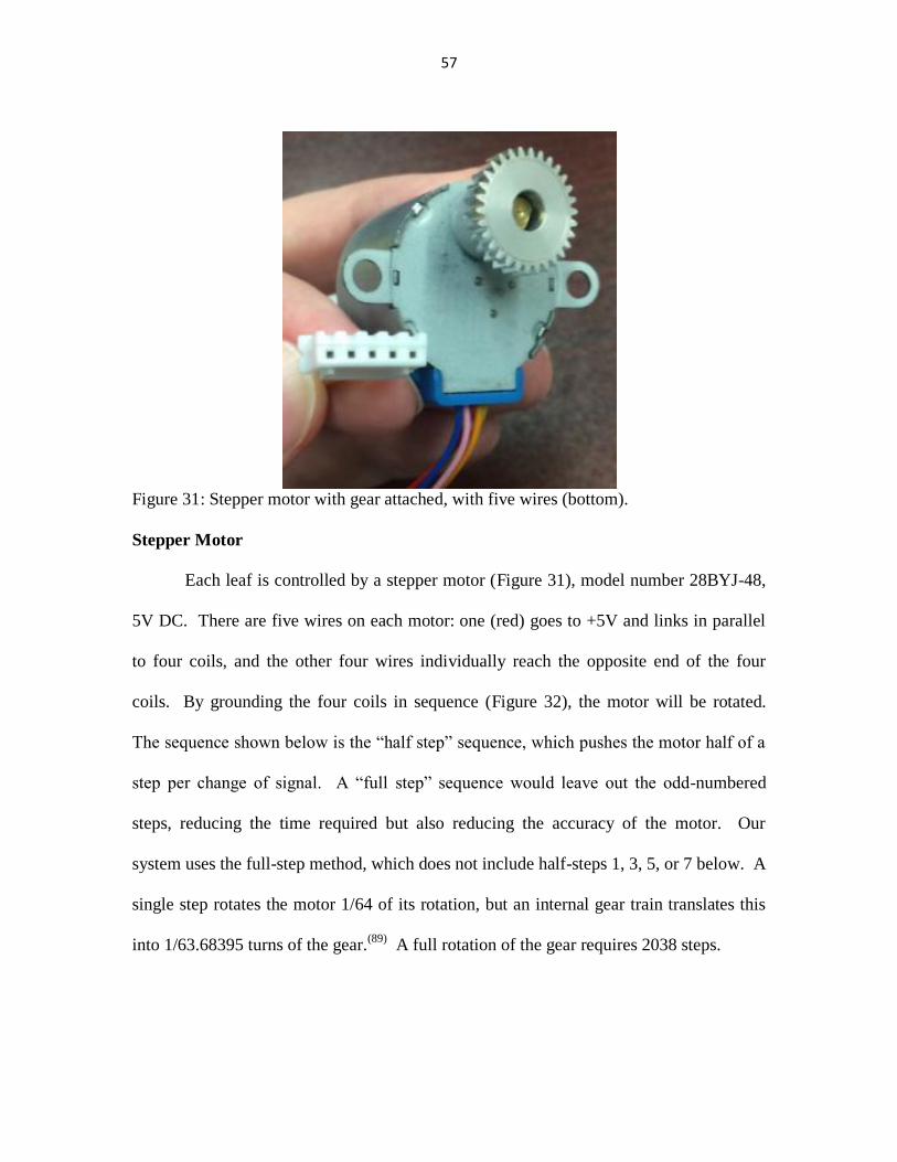
Stepper Motor ___________________________________________________57

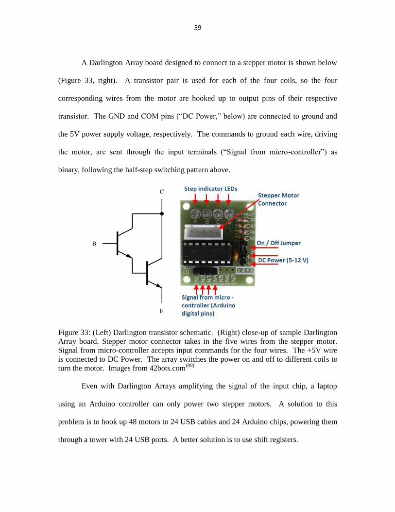
Darlington Array _________________________________________________58

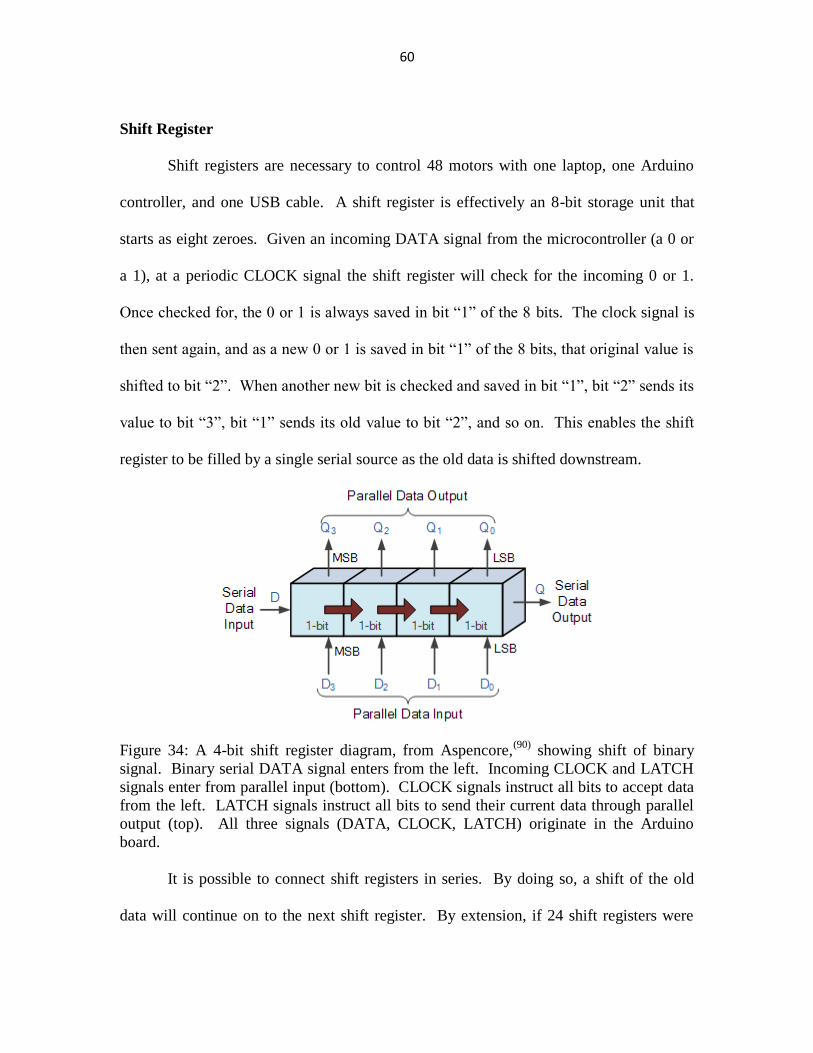
Shift Register ____________________________________________________60

Circuit Board ____________________________________________________62

Arduino Microcontroller ___________________________________________63

Qt Software _____________________________________________________64

Power Supply ____________________________________________________67

Control System Commissioning ______________________________________68

Circuitry Issues and Fixes __________________________________________69

Chapter 7 “Phantoms and Treatment Planning” _______________________________71

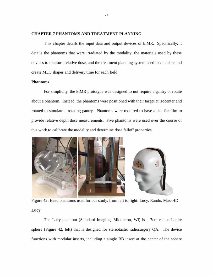
Phantoms _______________________________________________________71

Lucy ___________________________________________________________71

Rando __________________________________________________________72

vii

Max-HD ________________________________________________________73

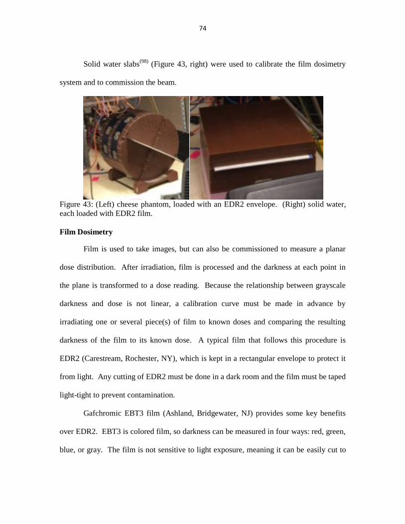
Cheese Phantom__________________________________________________73

Solid Water______________________________________________________73

Film Dosimetry __________________________________________________74

Treatment Planning System _________________________________________76

Planning Techniques ______________________________________________77

Beam on Time Calculation__________________________________________79

MLC Shape Export ________________________________________________80

Plan Summary ___________________________________________________81

Chapter 8 “Proof of Concept of kIMR” ______________________________________82

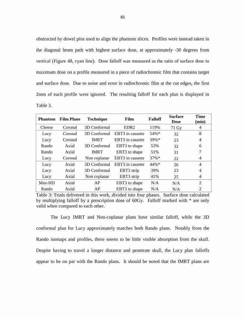
Falloff __________________________________________________________82

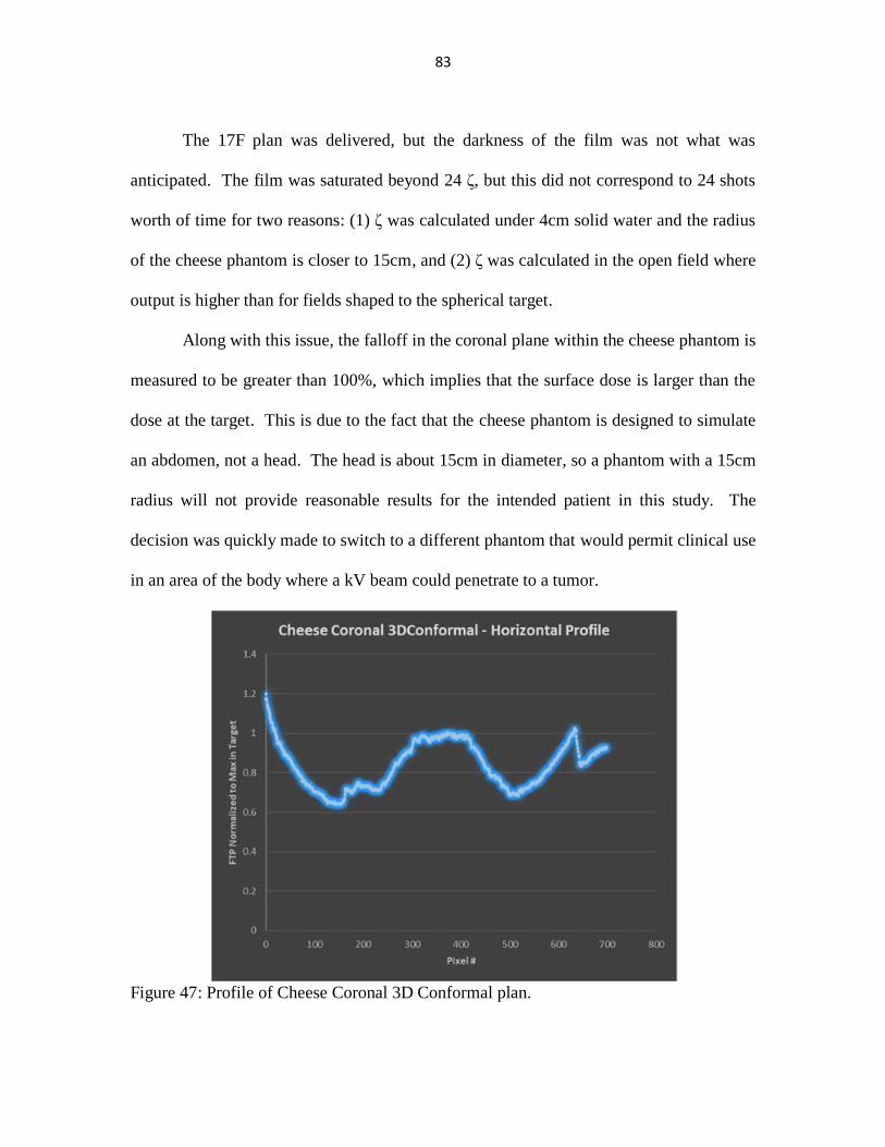
Phase 1: Cheese Phantom __________________________________________82

Phase 2: Lucy Coronal and Rando ___________________________________84

Phase 3: Lucy Axial _______________________________________________88

Phase 4: Single-field Skull __________________________________________89

Evaluation of Beam Penetration and Skin Toxicity _______________________91

Chapter 9 “Dose Falloff, CERT, and Future Feasibilities” _______________________92

Low-cost Conformal kV ____________________________________________92

Penetrability of kIMR ______________________________________________93

Risk to the Skin and Skull ___________________________________________93

Plausibility of GBM Contrast Enhancement ____________________________94

Appendix ______________________________________________________________97

viii

References ____________________________________________________________102

Abstract ______________________________________________________________115

Autobiographical Statement ______________________________________________117

ix

LIST OF TABLES

Table 1: ζ calibration settings ______________________________________________33

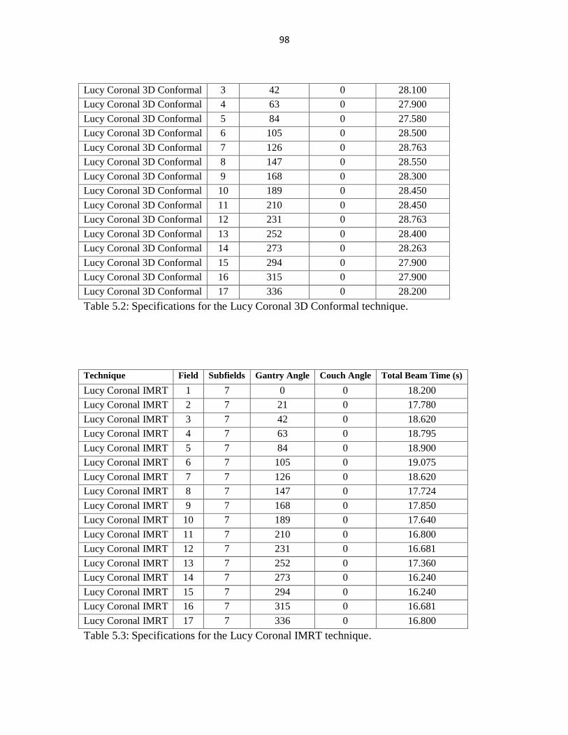
Table 2: Summary of delivered plans ________________________________________81

Table 3: Trials delivered by phase __________________________________________85

Table 4: Possible beam delivery times _______________________________________97

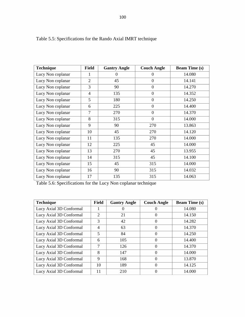
Table 5: Specifications for delivery techniques ________________________________97

x

LIST OF FIGURES

Figure 1: Multi-Leaf Collimator _____________________________________________2

Figure 2: Boron Neutron Capture ____________________________________________5

Figure 3: Dominant Photon Interactions _______________________________________9

Figure 4: The Auger Effect ________________________________________________11

Figure 5: Local Effect Model ______________________________________________12

Figure 6: Linear Quadratic Model __________________________________________14

Figure 7: LEM – AuNP Predictions _________________________________________16

Figure 8: Lycurgus Cup __________________________________________________17

Figure 9: TEM AuNP Sizes _______________________________________________19

Figure 10: Experimental Setup _____________________________________________25

Figure 11: Pantak 300 DXT _______________________________________________26

Figure 12: WSU Neutron Cyclotron _________________________________________28

Figure 13: Indico 100 Controller ___________________________________________30

Figure 14: Setup Accessories ______________________________________________33

Figure 15: CAD-CAM-CNC_______________________________________________35

Figure 16: Mills & Endmills _______________________________________________36

Figure 17: Tormach CNC _________________________________________________37

Figure 18: Brass MLC Model ______________________________________________38

Figure 19: Brass Leaves __________________________________________________39

Figure 20: Penumbra Measurement _________________________________________41

Figure 21: Leaf Straightening Jig ___________________________________________42

xi

Figure 22: Tungsten Carbide ______________________________________________43

Figure 23: 3D Printer ____________________________________________________46

Figure 24: Gear Rack ____________________________________________________47

Figure 25: Comb ________________________________________________________48

Figure 26: Rod Guide ____________________________________________________49

Figure 27: Circuitry Mounts _______________________________________________50

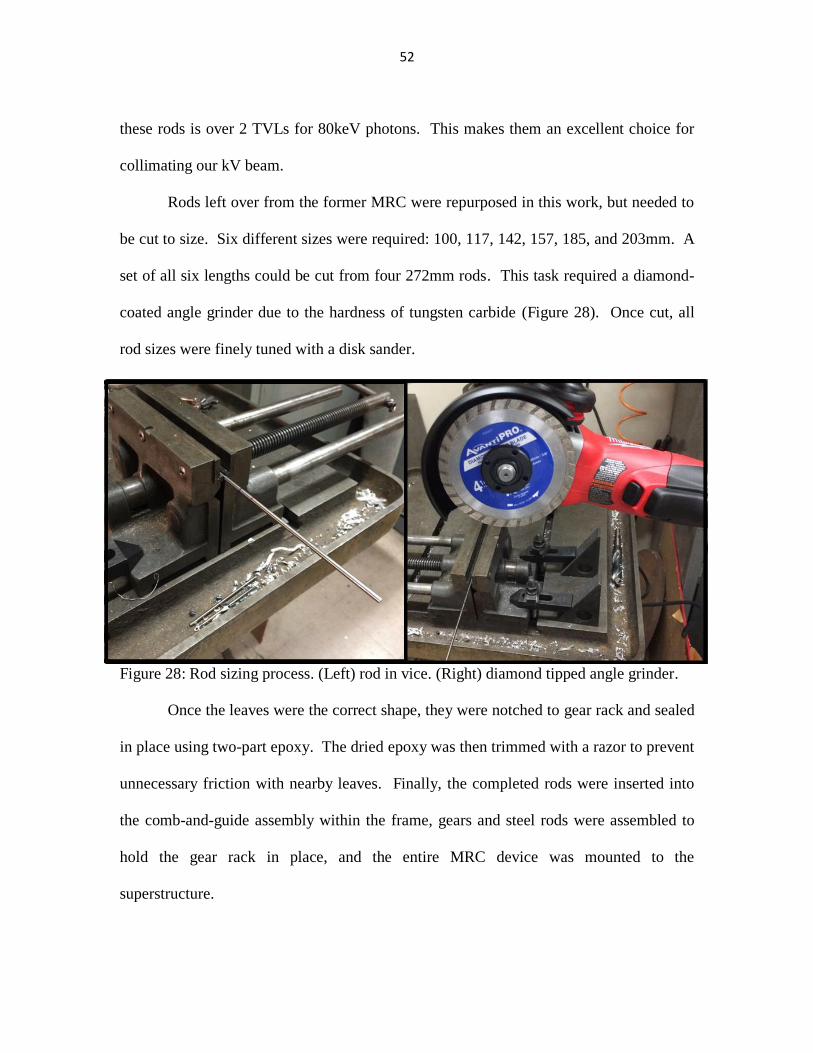
Figure 28: Rod Sizing ____________________________________________________52

Figure 29: EDR2 Alignment _______________________________________________55

Figure 30: Control System Diagram _________________________________________56

Figure 31: Stepper Motor _________________________________________________57

Figure 32: Switching Sequence ____________________________________________58

Figure 33: Darlington Array Schematic ______________________________________59

Figure 34: Shift Register Diagram __________________________________________60

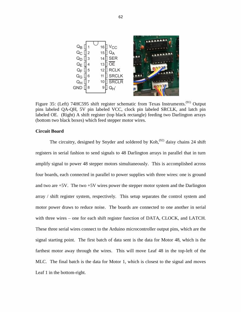
Figure 35: Shift Register Schematic _________________________________________62

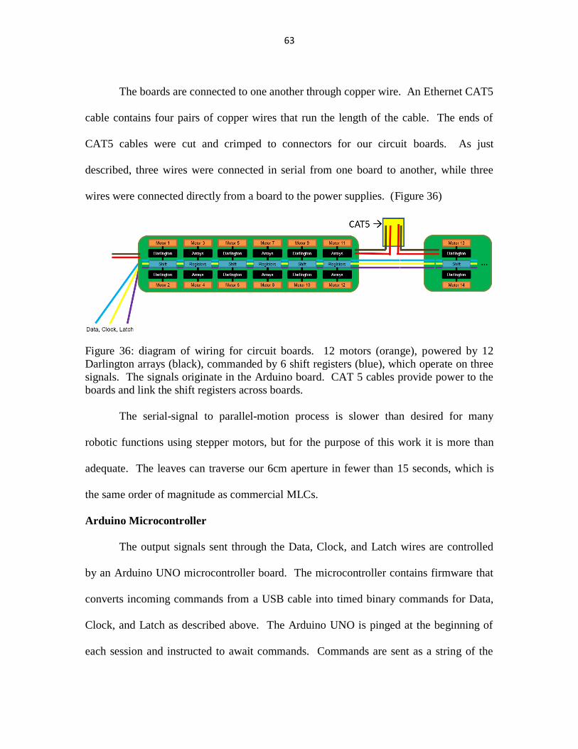
Figure 36: Circuit Board Diagram __________________________________________63

Figure 37: Arduino UNO Microcontroller ____________________________________64

Figure 38: Initialized MLC ________________________________________________65

Figure 39: Qt GUI _______________________________________________________66

Figure 40: Laptop Wiring _________________________________________________67

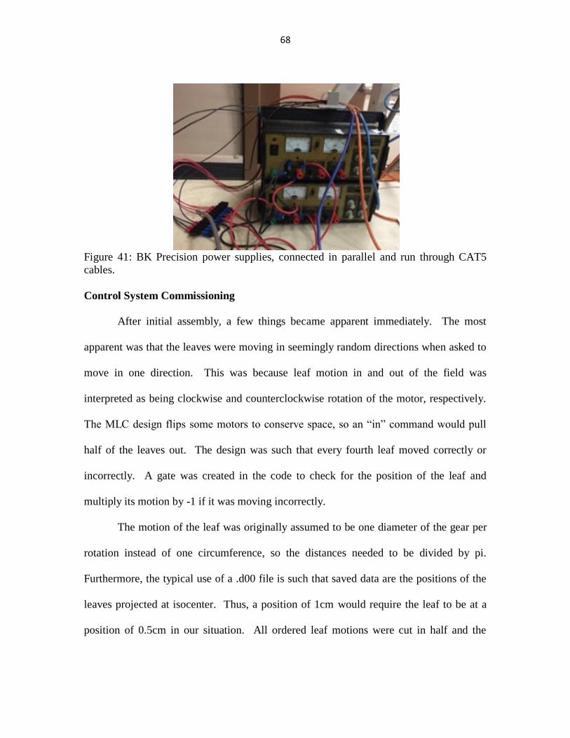
Figure 41: Power Supplies ________________________________________________68

Figure 42: Head Phantoms ________________________________________________71

Figure 43: Cheese Phantom and Solid Water __________________________________74

xii

Figure 44: EBT3 Calibration ______________________________________________75

Figure 45: Eclipse kIMR vs TrueBeam ______________________________________77

Figure 46: Non-coplanar Fields ____________________________________________79

Figure 47: Cheese Profile _________________________________________________83

Figure 48: Isomaps ______________________________________________________86

Figure 49: Lucy Profile ___________________________________________________87

Figure 50: Lucy Strip Inserts ______________________________________________89

Figure 51: Single field PDDs ______________________________________________90

1

CHAPTER 1 TREATMENT OF GLIOBLASTOMA MULTIFORME

Cancer treatment is often divided into three categories: surgery, chemotherapy,

and radiation therapy. This dissertation is a work of medical physics, concentrating in

radiation therapy physics. This chapter briefly introduces radiotherapy, the motivation

for this study, the current state of research, and how this work contributes to the field.

Radiotherapy

The first study of therapeutic radiation was published in 1902,(1)

only seven years

after the discovery of radiation itself. As accelerator technology advanced, the energy of

photons used for radiotherapy steadily increased. Grenz ray tubes (<20keV) gave way to

superficial treatments (50-150keV), which advanced to orthovoltage (150-500keV),

supervoltage (500-1000keV), and eventually megavoltage radiotherapy (>1000keV or

>1MeV).(2)

The discovery of cobalt-60, which naturally emits 1.17 and 1.33MeV

photons, led to a loss of popularity for x-ray beams. Their resurgence was only realized

after the accelerators of the mid-century reached the MeV range.

There are significant advantages to treating a patient with megavoltage

radiotherapy. The most important advantage is that megavoltage photons spare the skin

at their entry point, permitting escalation to modern prescription doses. A second

advantage is that higher energy photons are more penetrating than lower energy photons,

which enables conformity to a deep target while sparing healthy tissue. Finally, higher

energy photon beams penetrate high atomic number (high-Z) media, such as bones, more

easily than lower energy photon beams. Because of these advantages, typical clinical

photon beams have high energies, with maximum energies usually ranging from 6 MeV

2

to 18 MeV. However, the low penetrability of kilovoltage beams through high-Z media

could be a missed opportunity.

The vast majority of radiotherapy beams are shaped to conform to a target and

spare healthy tissue through the use of a multi-leaf collimator (MLC), which forms a

customizable 2D block to shield healthy tissue from radiation (Figure 1). An MLC

permits treatments from several angles without manual block replacement and also opens

the door to forward-planned field-in-field therapy and inverse-planned intensity

modulated radiotherapy (IMRT). IMRT produces the most conformal treatments in the

field, often with the shape of the MLC changing while the beam is on, though it is

simpler to plan with a step-and-shoot delivery. IMRT is the most frequently chosen

technique for tumors in the prostate, lung, esophagus, and head-and-neck region, as well

as partial brain treatments such as those for Glioblastoma Multiforme.

Figure 1: Diagram of Multi Leaf Collimator (MLC) in radiotherapy, from Romeijn et

al.(3)

3

Glioblastoma Multiforme

Cancer is the second leading cause of death in the United States,(4)

and few

cancers are as deadly as Glioblastoma Multiforme (GBM). GBM is another name for a

grade 4 astrocytoma, a highly malignant brain tumor that, while a rare primary diagnosis,

accounts for about 15-20% of tumors in the central nervous system.(5)

Only about 2% of

patients diagnosed with GBM survive for three years,(6)

making this a candidate for

particularly unconventional research and solutions. The standard of care for GBM is to

remove the tumor with surgical resection,(7)

but total resection of a GBM is only achieved

in about 30% of cases.(8)

To treat residual tumor and prevent local recurrence, the

surgical cavity is treated with a combination of chemotherapy (specifically oral

temozolomide(5,7)

or surgically-implanted carmustine wafers(5,9)

) and radiation therapy

(specifically, IMRT with megavoltage photons). Despite these efforts, GBM has an

unusually high rate of local recurrence even when total resection is achieved.(10)

This

could be due to the presence of radioresistant cancer stem cells,(11)

from which cancer can

respawn.

The possible solution to local recurrence is to increase the dosage of chemo- and

radiotherapies at the tumor site to target cancer stem cells and residual malignant tissue,

but a simple increase in dosage leaves many issues unaddressed. The brain is protected

from dangerous chemicals in the bloodstream by a semi-permeable membrane named the

Blood-Brain Barrier (BBB). Designing a chemotherapy drug to penetrate the BBB is a

difficult task.(12)

Additionally, GBM cavity radiotherapy escalation has been found to

have no additional therapeutic benefit beyond 60Gy.(13,14)

In fact, Chan et al found that

4

they were doing more harm than good beyond this point.(14)

Other radiotherapy dose

escalation studies to 70Gy have yielded various results.(15-17)

Thus, GBM radiotherapy

advancements have been refocused to dose enhancement.

Dose enhancement is a relative measure of the radio-biological effect (RBE) of

radiation treatment compared to a standard, which is usually cobalt-60 or a 250 kVp

photon beam. Instead of simply increasing the amount of dose delivered to the body, a

more effective dose is delivered. The RBE of an experimental therapy is equal to:

Some ways to increase RBE involve combating hypoxic tumors through the use

of oxygen enhancement and hypothermia.(18)

A more straightforward way to increase

RBE is to apply heavy charged particles, such as protons or alpha particles. A Phase II

study confirmed survival benefit at 90Gy using a combined photon-proton treatment with

BID fractionation.(19)

Another delivery mechanism for heavy charged particles, Boron

Neutron Capture Therapy (BNCT), is an encouraging option for the treatment of

GBM.(20,21)

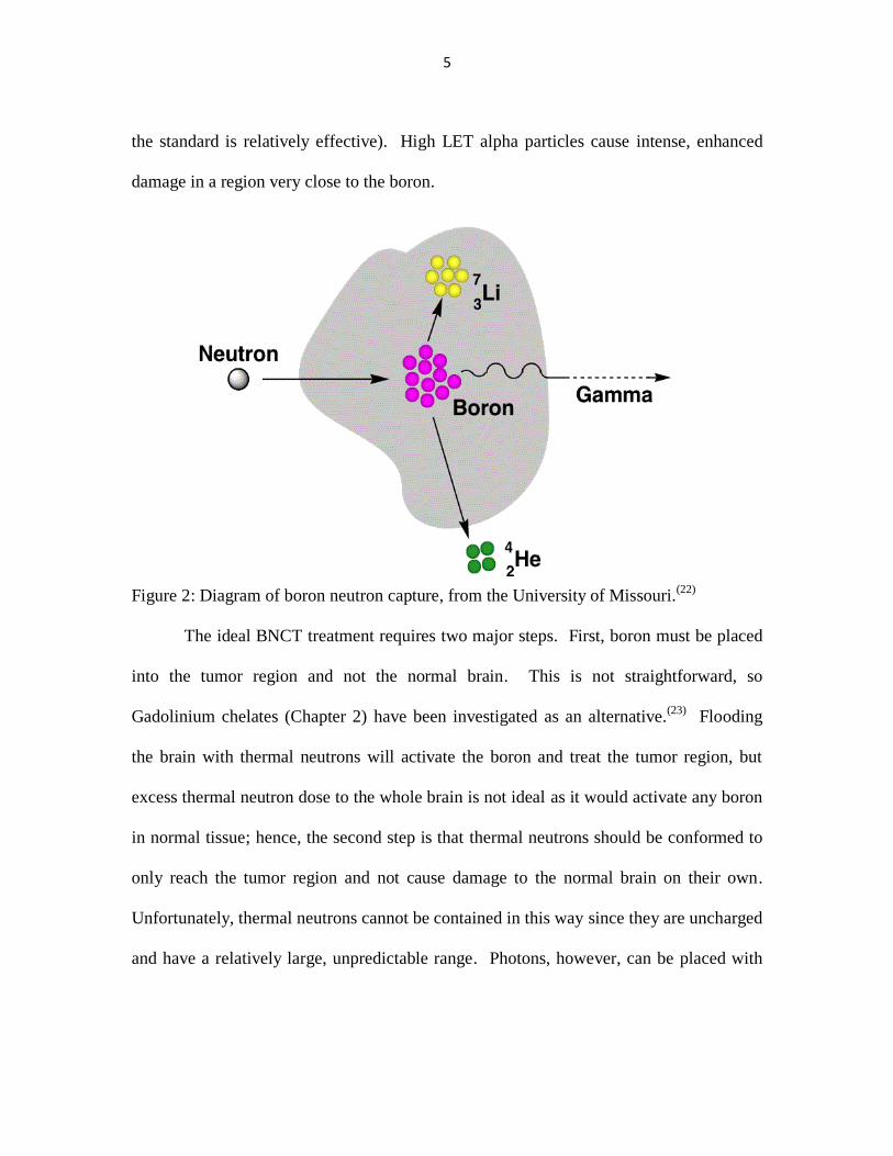
Boron Neutron Capture Therapy

BNCT requires the placement of boron into and around the tumor region. The

entire brain is then flooded with thermal (low-energy) neutrons. Boron has a high

interaction probability with thermal neutrons, and the interaction results in the emission

of a very short range alpha particle and Li-7 ion (Figure 2, in green) that both have high

linear energy transfer (LET). RBE increases with LET (until ~100keV/µm, after which

5

the standard is relatively effective). High LET alpha particles cause intense, enhanced

damage in a region very close to the boron.

Figure 2: Diagram of boron neutron capture, from the University of Missouri.(22)

The ideal BNCT treatment requires two major steps. First, boron must be placed

into the tumor region and not the normal brain. This is not straightforward, so

Gadolinium chelates (Chapter 2) have been investigated as an alternative.(23)

Flooding

the brain with thermal neutrons will activate the boron and treat the tumor region, but

excess thermal neutron dose to the whole brain is not ideal as it would activate any boron

in normal tissue; hence, the second step is that thermal neutrons should be conformed to

only reach the tumor region and not cause damage to the normal brain on their own.

Unfortunately, thermal neutrons cannot be contained in this way since they are uncharged

and have a relatively large, unpredictable range. Photons, however, can be placed with

6

high conformity into deep tumors using techniques such as IMRT. Contrast Enhanced

Radiotherapy (CERT) is a parallel to BNC that uses photons instead of neutrons.

Contrast Enhanced Radiotherapy

CERT commonly involves the implantation of iodine,(24)

gadolinium,(25)

gold

nanoparticles(26)

(AuNPs), or other high-Z materials into a target region followed by

irradiation with low-energy photons. As noted above, high energy photons penetrate

high-Z materials readily; in contrast, low-energy photons interact more often in high-Z

materials due to the photoelectric effect.(27)

This effect has a high rate of transfer of

photon energy into electron energy through Auger electron showers(28)

(Chapter 2). This

increases the LET and the RBE in the region.(27)

Current research into CERT utilizes tunable, monochromatic microbeam

radiation from synchrotrons to improve beam penetration and hone in on desirable K-

edge photon energies (Chapter 2). Clinical microbeam use is only available in a few

centers worldwide, none of which are in North America.(29)

Synchrotrons are high-

demand, prohibitively expensive sources with circumferences on the order of hundreds of

meters and, while powerful, the field size of these devices is on the order of fractions of a

millimeter.(29)

This is insufficient for a tumor the size of a GBM. The use of CT imagers

as therapeutic devices has also been investigated with the addition of iodine contrast(30)

and with modifications to the beam(31)

to perform quasi-monochromatic therapies. Each

of these methods can adhere to the target shape and produce an excellent theoretical dose

distribution in the brain, but their fields are highly focused and require clinically

significant delivery times due to tube cooling.(31)

7

There are many clinical concerns surrounding the use of CERT. Because this

technique requires treating with low-energy photons, there will be an increase in skin

dose. Reactions to skin dose are known to begin at approximately 20Gy for typical

2Gy/fx treatments.(32)

Furthermore, in brain treatments specifically, the skull will need to

be penetrated. Due to the very mechanism of which CERT takes advantage, the skull

will hinder any low-energy dose delivery to the brain due to its high effective atomic

number (approximately 12.3, compared to the effective atomic number of 7.5 in

tissue(33)

). The dose threshold for necrosis in the skull is known to be about 60Gy.(34)

Any increase in dose enhancement at the target will need to outweigh the increased dose

to the skin and skull.

In addition, low energy photons are attenuated more readily than high energy

photons, meaning the beam will not reach deep tumors as easily. Any dose from this

poorly penetrating beam that does reach the target, plus any dose enhancement, must

outweigh the increased dose to the skin and skull.

Kilovoltage Intensity Modulated Radiotherapy

In summary, the primary issues with using kilovoltage (kV) radiotherapy to treat a

large, deep tumor with CERT are fourfold: poor beam penetration, high dose to skin and

bone, expensive radiation delivery mechanisms and difficulty getting contrast into the

target. However, if treatment is exclusively in the brain, the distance to a tumor is

reduced compared to distances to deep tumors in the rest of the body. Also, the increased

RBE from CERT could potentially offset the increased dose to the skin and skull. The

primary questions are:

8

1) Can a conformal kV CERT modality be created at low cost?

2) Is it plausible to deliver a contrast agent to a GBM tumor and not surrounding

normal tissue?

3) Is a clinically acceptable plan deliverable using kV photons?

4) Would a clinically acceptable plan be toxic to skin or skull?

The purpose of this work is twofold: (1) to examine CERT literature to determine

the feasibility of GBM CERT with a conformal kV beam, and (2) to evaluate the

penetration capabilities of conformal kV radiotherapy in the brain. To these ends,

Chapter 2 details the current state of the field with regard to GBM CERT, and Chapters

3-7 detail the design, construction, and testing of our new modality: kilovoltage intensity

modulated radiotherapy (kIMR). In short, we created a low-cost in-house Multi-Rod

Collimator (MRC) and mounted it to the portal imaging tube of a decommissioned

neutron cyclotron to determine the penetration characteristics of a kV beam in the brain.

Chapter 8 details the final experiments into this modality, which include 17-field 3D

conformal and intensity modulated plans on rotating phantoms, utilizing radiochromic

film dosimetry. Tasks required to accomplish this ranged from 3D printing a flattening

filter to CNC milling brass leaves en masse, cutting tungsten carbide rods with an angle

grinder, learning basic robotics, and reprogramming an in-house GUI/control system.

This work aims to justify future pursuits of this modality in the treatment of GBM.

9

CHAPTER 2 CONTRAST ENHANCED RADIOTHERAPY

Photons deposit their energy into a medium in three important ways, each of

which has different biological impact in tissue. The probability of each mechanism

(Figure 3) depends on the energy of the incident photon and the atomic number of the

medium.(27)

Contrast enhanced radiotherapy (CERT) takes advantage of the benefits

gained when using low energy photons to irradiate high atomic number materials. In

short, CERT first adds a high atomic number medium to the target region so that

radiation is enhanced by making photoelectric interactions more likely to happen. The

mechanisms of energy transfer are described below, followed by a discussion on cell

survival models and contrast agents of interest, with a focus on gold nanoparticles.

Figure 3: Dominant photon interaction mechanisms, from Attix.(27)

Photoelectric

interactions are dominant for higher Z, lower incident photon energy.

10

Megavoltage and Kilovoltage Photon Interactions

The three most important modes of photon interactions in radiation therapy are

Compton scattering, the photoelectric effect, and pair production. Pair production will

not be considered because it requires an incident photon to have at least 1.022MeV of

energy, which will not be possible in this work.

Compton scattering is the dominant interaction mechanism in the range of photon

energies used in megavoltage radiotherapy. In Compton events, photons interact with an

electron in the outer shells of an atom. The outer shell electrons have such low binding

energy compared to the incident photon energy that they are considered free electrons.

Due to conservation of momentum and energy, the photon must retain some portion of its

initial energy, the amount of which is calculable using the Klein-Nishina cross

sections.(27,35)

The remaining energy remains nearby (in the kinetic energy of the free

electron) and contributes to dose at the interaction site (minus any radiative loss). The

critical point is that this amount must be less than 100% of the initial photon energy.

Photoelectric interactions(36)

are the dominant interaction mechanism in

kilovoltage radiotherapy and imaging, especially in high-Z materials. A keV photon that

interacts with a tightly bound inner shell electron does not have such high energy that the

electron is considered free, so the nucleus contributes in conservation of momentum and

energy. As a result of this, the photon is completely absorbed by the inner shell electron,

which is then ejected. The entirety of the incident photon energy, less the inner shell

binding energy, is released as kinetic energy through the ejected electron. That lost inner

shell binding energy is accounted for by a cascade of outer shell electrons that fill the

11

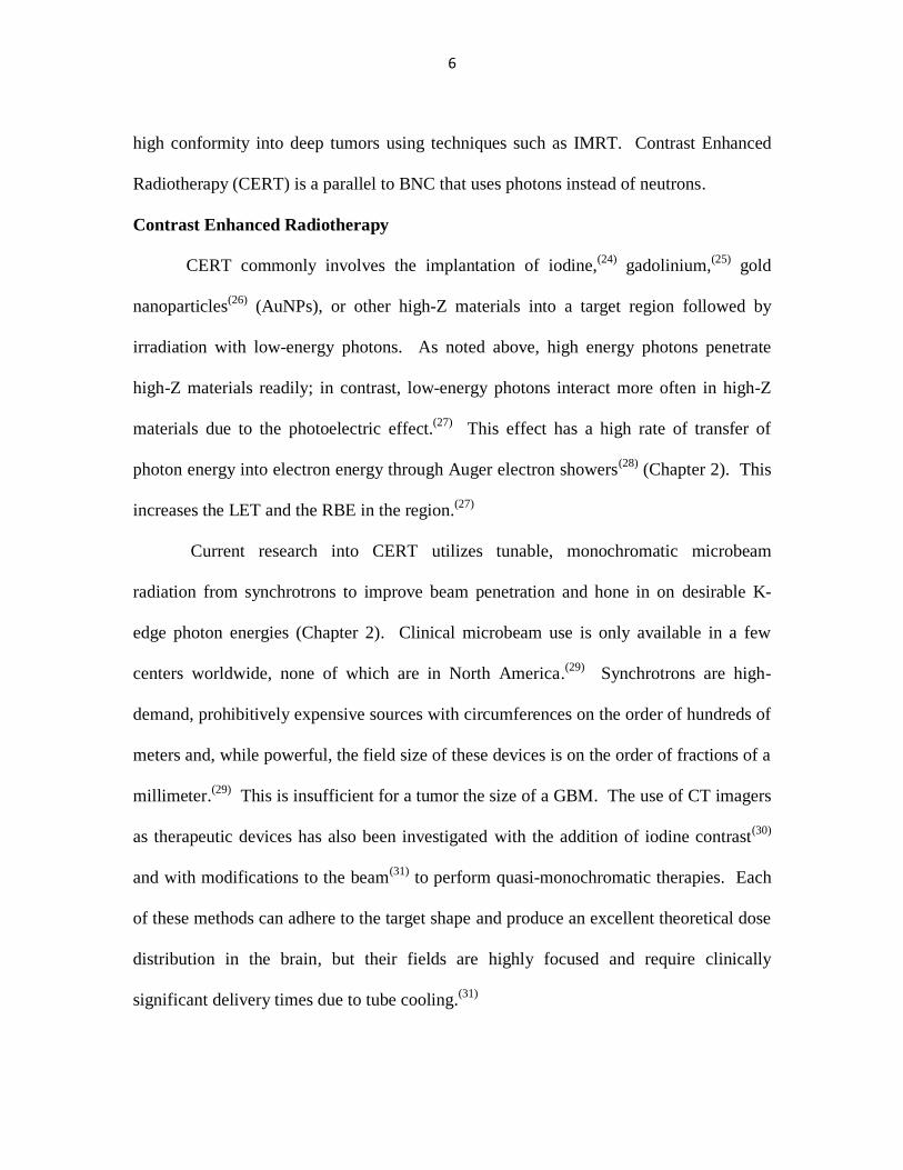
energy gap left by the ejected inner shell electron. The energy released from these

transitions is emitted either as a characteristic x-ray or by ejecting several outer shell

electrons. These ejected electrons are called Auger electrons(28)

and each have very low

energy and, by extension, a very short range. Through the Auger mechanism, 100% of

the incident photon energy can be converted into charged particle kinetic energy and

contribute to dose very near the interaction site. (Figure 4).

Figure 4: The Auger effect. Low energy electrons are released instead of photons from

photoelectric interactions. Image from Nave.(37)

12

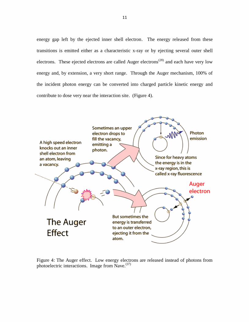
Photoelectric interactions become more probable when photons interact with

materials that have high electron binding energies in the inner shell. Binding energy of

the inner shell increases with the atomic number of the nucleus, meaning that high-Z

materials are more likely to have photoelectric interactions that convert a higher fraction

of incoming energy into charged particle kinetic energy than the Compton interaction.

Likewise, photoelectric interactions become more probable when photon energy exceeds

the binding energy of these electrons, known as the “K-edge” (See Figure 5, right).

Figure 5: Local effect model findings(38)

suggest (left) increased RBE from AuNP of

smaller size, and (right) increased RBE from lower energy photons, with a spike at the K-

edge of gold (80 keV).

Photoelectric interaction probability increases proportional to the quantity (Z/E)3.

That is, there is a cubic dependence with atomic number and an inverse cubic dependence

on incident photon energy. For a given photon energy E, the relative probability of

photoelectric interaction in two media “a” and “b” is equal to (Za/Zb)3. Combining these

effects into low energy CERT will not just increase the dose to the target by increasing

interaction probability, but the interactions that do occur have an increased fraction of

13

their energy deposited as high-LET Auger electron dose. Through CERT, the

photoelectric effect increases both dose to tissue and radiobiological effect.

Quantitative Measures of Dose Enhancement

Formalism has been defined in the literature to describe dose enhancement. Some

quantitative measures of dose enhancement are the Dose Enhancement Factor (DEF),

Sensitizing Enhancement Ratio (SER), and Surviving Fraction (SF). These follow the

same basic principle and structure as RBE (Chapter 1).

Dose enhancement factor (or fraction) is defined as the dose required to produce

an effect divided by the dose required to achieve the same effect in the presence of a

drug. This is very similar to the sensitizing enhancement ratio, which is dose required to

achieve an effect divided by the dose required to produce the same effect in the presence

of a sensitizer.

Surviving fraction is a ratio of the cells that survive a dose of radiation divided by

a control. This is often the metric used to create the above ratios when experimenting in

vitro. Surviving fraction is used to model cell survival.

Linear Quadratic Model

Cell survival differs based on the type of radiation delivered. For a specific type

of radiation (energy and modality, say 6MV photons) semi-log plots are frequently

created of the surviving fraction of cells as a function of dose delivered. These plots can

14

be fitted to a zero-constant second order polynomial with more weight in the linear or

quadratic term, depending on the cell line and the specific kind of radiation.(18)

This is

the basis of the Linear Quadratic (LQ) model. Higher LET radiation doses are more

linear and lower LET radiation is more quadratic. The “bendiness” of the curve (Figure

6) is determined by a constant of linearity (α) and its quadratic counterpart (β), which

solves to the following equation for surviving fraction (S) over dose (D):

Figure 6: LQ plot from RadiologyKey.(39)

High LET radiations have a more linear cell

survival curve with a high α component, while low LET curves have a more quadratic

shoulder with a high β component.

Much of the experimental cell survival data in the literature can be predicted

using Monte Carlo modeling based on macroscopic cell survival curves. However, there

15

are exceptions that include cellular response to kilovoltage CERT using gold

nanoparticles,(38)

leading to investigations using alternative models.

Local Effect Model

According to the authors of the Local Effect Model(40)

(LEM), the LQ model

assumes a macroscopic view of the cell that falls apart at the nanometer scale. Gold

nanoparticle CERT, for example, operates through Auger showers originating in what are

approximately 2nm diameter spheres.

Within a cell containing heterogeneous exposures, the LET and RBE are, strictly

speaking, a function of location in the cell. The LEM assumes that cells die from the

random formation of a number of lesions “N,” with surviving fraction expressed as:

The model then splits the cell into a large number of voxels and calculates, using

radial dose profiles and Monte Carlo code, the differential probability of a lesion forming

in each voxel. These are calculated using the LQ alpha and beta values of photons in the

absence of a contrast medium. The model assumes that N is the integral of these

differential probabilities.(41)

This allows for the effect of a very high LET interaction,

such as from a gold nanoparticle, to be more accurately modeled over an entire cell using

low-LET cell survival data.

The radiobiological enhancement of a gold nanoparticle is not a constant that

affects the dose compared to a standard at individual dose points, but can be modeled as a

single constant that increases the linearity of the cell survival curve. That is, the

16

enhancement increases the α quantity in the LQ model. This agrees with findings that

experimentally found an increase in survival curve linearity.(38)

Predictions from macroscopic models suggest(42,43)

that gold nanoparticle

concentrations on the order of 1% would lead to a DEF of approximately 2, but

experimental data have shown that far smaller concentrations are required to reach this

effect. McMahon et al(38)

used the LEM to provide the first theoretical justification for

this data (Figure 7).

Figure 7: Local effect model predictions(38)

with gold nanoparticles. Solid line plotted

using “No Gold” cell survival data using LQ model. This information was used to run an

LEM prediction of dose enhancement from AuNPs with a known concentration and size

in the same cell line. The results (dashed line) match experimental data (“With Gold”).

17

Gold Nanoparticles

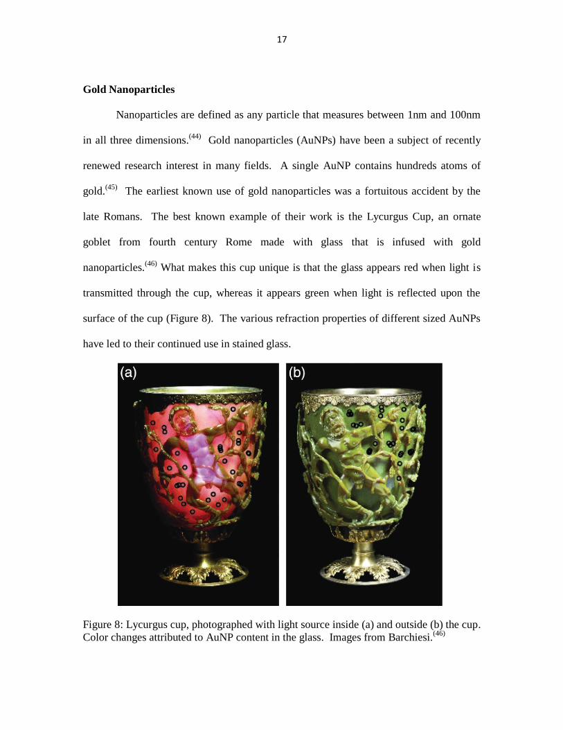
Nanoparticles are defined as any particle that measures between 1nm and 100nm

in all three dimensions.(44)

Gold nanoparticles (AuNPs) have been a subject of recently

renewed research interest in many fields. A single AuNP contains hundreds atoms of

gold.(45)

The earliest known use of gold nanoparticles was a fortuitous accident by the

late Romans. The best known example of their work is the Lycurgus Cup, an ornate

goblet from fourth century Rome made with glass that is infused with gold

nanoparticles.(46)

What makes this cup unique is that the glass appears red when light is

transmitted through the cup, whereas it appears green when light is reflected upon the

surface of the cup (Figure 8). The various refraction properties of different sized AuNPs

have led to their continued use in stained glass.

Figure 8: Lycurgus cup, photographed with light source inside (a) and outside (b) the cup.

Color changes attributed to AuNP content in the glass. Images from Barchiesi.(46)

18

AuNP solutions have also been used in 17th

century alchemical and hermetic

philosophy(47)

and, quite recently, as an environmentally conscious alternative to

conventional ceramic coloring.(48)

Sengani et al list 15 ways to synthesize AuNPs,

ranging from conventional chemical reduction and laser ablation to synthesis mediated by

boiling citrus pulp.(49)

Gold nanoparticles are used throughout the sciences for everything from

nanoscale solar energy absorption(50)

to carbon monoxide conversion.(51)

In medicine,

gold nanoparticles are being researched for imaging contrast, radiosensitization, and as a

mechanism for drug delivery. Drugs can be adhered to the surface of AuNPs to aid in

bringing the treatment molecule to the correct site.(52)

For example, tumor cells can be

directly targeted because they overexpress receptors of the tissue factor (TF) protein.(52)

AuNPs have been fitted with TF and selectively absorbed by nasopharyngeal carcinoma

cells through endocytosis.(52,53)

Very small AuNPs (1-2nm) have been found to penetrate the blood brain barrier

in mice,(54)

with a maximum concentration reached at 6-16 hours post-injection before a

sharp decline.(54)

BBB permeability for AuNPs has been found to increase with the use

of focused ultrasound(12)

and ultrasound contrast media. Once through the BBB, AuNPs

can accumulate in solid tumors due to leaky vasculature.(55)

Tumor targeting can thus be

achieved without the use of a targeting ligand, which will lead to tumors selectively

receiving more dose than healthy tissue.

The review by Haume et al regarding gold nanoparticles in radiotherapy(55)

highlights customizable parameters of consequence. The following sections detail these

19

parameters in the order from Haume(55)

and gives recommendations for optimization of

AuNP setup for kilovoltage photon radiotherapy in the brain. The four customizable

parameters are: size, concentration, surface charge, and coating. Changes in these

parameters affect the nanoparticle delivery mechanism and toxicity. Many of the

following tradeoffs also apply to gadolinium nanoparticles, but gold will be the focus.

AuNP Size

To avoid long term side effects, it is best to keep AuNPs from accumulating in

vital organs such as the heart and liver. To achieve this, all nanoparticles should leave

the body within a few days.(55)

This is generally done through renal clearance.(56)

Studies

have shown that the size of a gold nanoparticle (Figure 9) affects renal clearance

probability.(57,58)

Nanoparticles greater than 10nm in diameter are more likely to be

captured by the liver, while those less than 6nm are usually eliminated independent of

charge. Intermediate particles (6-10nm) are eliminated more quickly when positively

charged.(56)

Figure 9: TEM images of gold nanoparticles of various sizes, from Sigma-Aldrich.(59)

While a small size reduces toxicity, larger sizes (20-60nm) tend to have higher

direct uptakes in cells. Despite this, smaller cells can still accumulate due to an increase

in the enhanced permeability and retention (EPR) effect.(60)

Due to EPR, smaller

20

nanoparticles can be more evenly distributed throughout a larger tumor (like GBM) than

larger particles. This effect may counteract the lower uptake and faster elimination of

smaller particles.(61)

Further studies(38,62,63)

point to the therapeutic advantages of smaller

NPs since Auger interactions, intended to damage tissues, are more likely to deposit their

energy outside the nanoparticle. This effect may help to further offset the negative

effects of small sizes.

AuNP Concentration

Mesbahi et al determined that the concentration of AuNP in cells had more of an

impact on outcomes than the size of the particle.(64)

Brun et al found that the best

radiosensitivity was present at the highest measured concentration and at intermediate

values of size and photon energy.(65)

As stated above, the local effect model has

demonstrated that lower concentrations than previously predicted are necessary to

achieve a desired radiobiological effect. Thus, the concentration may not need to be as

high as predicted in earlier studies.

AuNP Surface Charge

A nanoparticle is a colloid, meaning it consists of hundreds of gold atoms

suspended in water (or another solute). The solute and the gold create a potential

difference, which is known as the surface charge. Surface charge can be adjusted prior to

use through the deliberate adsorption of ions and coating the exterior of the gold core

with specific ligands.

Two key effects occur as a result of positive or negative surface charge: uptake in

cells and tagging for removal by the immune system. The optimal charge of an AuNP is

21

not known, but a theoretical study(66)

showed that the mechanism of absorption depends

on the amount of charge. The lipid membranes in tumor cells that AuNPs must penetrate

are negatively charged, so positively charged particles will more readily penetrate these

barriers. Cancer cells have a structure called glycocalyx(67)

that is larger than in normal

cells and can be more negatively charged, permitting selective permeability of positively

charged AuNPs. Furthermore, positively charged particles induce membrane issues and

interfere with cell functions that cause pores in the membrane. These arguments suggest

that positively charged NPs are superior.

A tradeoff to consider with positively charged NPs is that they are more readily

targeted for clearance by the body, which will reduce their passive targeting

capabilities.(57)

A foreign object in the bloodstream will attract opsonin, a negatively-

charged antibody that tags the cell for clearance. This can be circumvented by coating

the NPs negatively to deflect these tags.

AuNP Coating and Targeting Mechanisms

The coating of a nanoparticle can be customized to generate specific effects that

aid in targeting a tumor. Tumor targeting can be passive or active, the goal of each being

to get AuNPs into the tumor. Passive targeting takes advantage of the porous, poorly

designed, high demand vasculature of a large tumor. Since tumors demand a large

quantity of blood and do not have a refined mechanism for vasculogenesis, nanoparticles

injected into the bloodstream can enter the tumor in larger quantities than normal tissue

and become trapped in vessels with abrupt stoppages and tight curves.(68)

Passive

22

targeting can also be improved by preventing the adsorption of opsonins, which can be

achieved by coating the nanoparticles appropriately.

Active targeting directly connects nanoparticles to the tumor cells by taking

advantage of receptors that are more present in tumor cells than in normal tissue.(69)

By

coating a nanoparticle in a chemical such as TF,(53)

the AuNP is drawn more often into

the overexpressed TF receptors of tumor cells. Many biological components have been

used for active targeting including, from Haume:(55)

antibodies, peptides, folates,

hormones, and glucose molecules.

It should be noted that the selected surface charge and coating of a nanoparticle

contributes to the mechanism and probability of tumor targeting. Coating can help

mediate the negative effects of surface charge and vice versa. Coating may, however,

absorb Auger electrons so that tumors are spared from AuNP dose enhancement. Gilles

et al(70)

investigated this mechanism and suggest a wispy coating for maximum effect.

Due to the large surface area of a gold nanoparticle, it is possible to unify the

effects of coating for active and passive targeting. Combination targeting combines the

two coatings mentioned above, permitting targeting of the TF receptors and repulsion of

opsonin. An optimal balance of the two has not been found, though a group did find that

passive targeting coatings can block the mechanism through which active targeting

coatings work.(71)

Passive coatings must then at least be in the minority in a combined

targeting coating. Other coatings include gadolinium chelate, which enhances MRI, and

the addition of imaging radionuclides such as Tc-99m.(57)

AuNP Toxicity

23

AuNP use will not be worthwhile if the nanoparticles are toxic to the normal

tissue. Commonly chosen characteristics to maximize radiological effect, without regard

to toxicity and based on the above qualifiers, are small particles (<5nm) in high

concentration with a positive charge and a coating that provides combination targeting.

At these sizes, AuNPs are chemically reactive. The mechanisms through which this

happens are unclear. There is suspicion that the particles propagate the “bystander

effect” to non-cancerous local tissues, which leads non-irradiated cells to undergo

apoptosis as if they were irradiated.(55)

Toxicity has been measured in different

proportions in different cancers, so the cancer itself may have a characteristic

dependency.

Toxicity studies are in progress and have been inconsistent. AuNPs are generally

nontoxic for diameters <5nm and >50nm, but toxic in between.(72)

Another study

suggests characteristic toxicity,(73)

with diameters of 3, 8, and 30nm measuring as toxic,

but not 5, 6, 10, 17,or 45nm.

Other Contrast Agents

Gadolinium (Gd) is frequently used as a contrast agent for brain imaging in MRI.

Gd works to reduce T1 and T2 relaxation times of surrounding protons by creating

oscillating magnetic fields due to its inherent paramagnetic properties.(74)

Its high atomic

number (64) makes it a candidate for CERT, however its photoelectric cross section is

approximately 50% of the photoelectric cross section of AuNP, meaning about twice the

external photon fluence would be needed to generate the same effect. Pure Gd is highly

toxic, so it is injected as a chelate to make renal clearance highly probable. Biological

24

half lives for Gd chelates range from 90-120 minutes. The primary benefit of Gd is that

Gd chelates are already FDA-approved for patient use in imaging studies,(75)

and they are

known to passively target GBM(76)

and penetrate the BBB when it is unhealthy.(76)

However, repeated use of Gd chelates has been found to leave permanent Gd

accumulation in its free and toxic form,(74)

so the FDA currently recommends(77)

that Gd

contrast agents not be used in repeated short-term scans when possible, especially not in

patients with kidney disease. Though no harm has been associated with long-term

accumulation of this Gd, it is uncertain whether the effect of a 30-fraction Gd injection

would be safe.

Iodine, as described in Chapter 1, is used as a contrast agent in CT and has been

investigated for use as a CERT agent. Iodine is internally regulated by the thyroid and

therefore safer than Gd. The quasi-monochromatic beam used in Jost(31)

was compared to

the normal CT polychromatic beam in a standard phantom and a gel phantom with iodine

homogeneously distributed. They claimed a DEF of 2.2-3.4 when compared to the

polychromatic beam with no iodine.(31)

Another study claimed a DEF from

concentrations of iodine measured with Fricke dosimetry as high as 4.8 based on very

high concentration in cells.(78)

The same group found no difference between iodine and

Gd contrast effect under equal concentrations under 110kVp photons and a 3.5mmAl

filter.(78)

Iodine is also approved for use as an imaging contrast agent in the brain, but its

atomic number (53) is also far lower than gold. For a given incident photon energy, the

necessary increase in incident photon fluence in iodine over gold to achieve the same

photoelectric interaction intensity (ZAu/ZI)3 is more than a factor of 3.

25

CHAPTER 3 X-RAY TUBE, SUPERSTRUCTURE, AND FILM CALIBRATION

This chapter describes the overall setup of our experiment and the logic that went

into its design. The kIMR modality is broadly overviewed, including the placement of

the X-ray tube, MLC, measuring device, and all necessary accessories. Then, the film

calibration procedure is explained for each type of film used in this study.

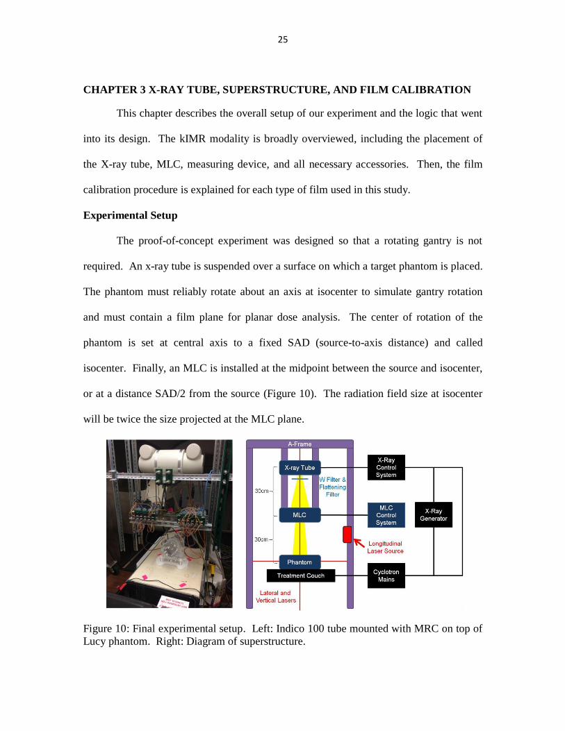
Experimental Setup

The proof-of-concept experiment was designed so that a rotating gantry is not

required. An x-ray tube is suspended over a surface on which a target phantom is placed.

The phantom must reliably rotate about an axis at isocenter to simulate gantry rotation

and must contain a film plane for planar dose analysis. The center of rotation of the

phantom is set at central axis to a fixed SAD (source-to-axis distance) and called

isocenter. Finally, an MLC is installed at the midpoint between the source and isocenter,

or at a distance SAD/2 from the source (Figure 10). The radiation field size at isocenter

will be twice the size projected at the MLC plane.

Figure 10: Final experimental setup. Left: Indico 100 tube mounted with MRC on top of

Lucy phantom. Right: Diagram of superstructure.

26

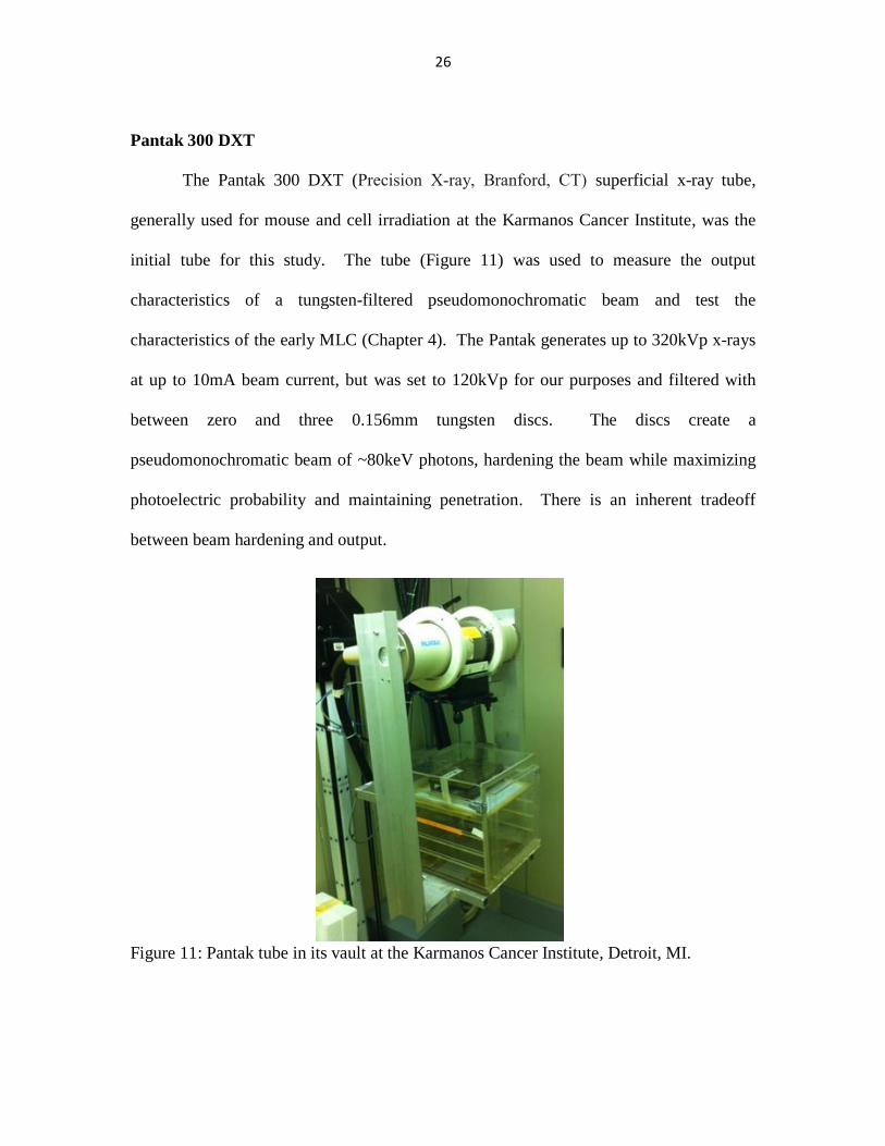
Pantak 300 DXT

The Pantak 300 DXT (Precision X‐ray, Branford, CT) superficial x-ray tube,

generally used for mouse and cell irradiation at the Karmanos Cancer Institute, was the

initial tube for this study. The tube (Figure 11) was used to measure the output

characteristics of a tungsten-filtered pseudomonochromatic beam and test the

characteristics of the early MLC (Chapter 4). The Pantak generates up to 320kVp x-rays

at up to 10mA beam current, but was set to 120kVp for our purposes and filtered with

between zero and three 0.156mm tungsten discs. The discs create a

pseudomonochromatic beam of ~80keV photons, hardening the beam while maximizing

photoelectric probability and maintaining penetration. There is an inherent tradeoff

between beam hardening and output.

Figure 11: Pantak tube in its vault at the Karmanos Cancer Institute, Detroit, MI.

27

As his thesis project, Jeff Riess(79)

characterized the Pantak tube for this project.

Riess directly measured many beam characteristics including profiles and PDD curves,

scatter factors using Cerrobend (Cerron Metal Products Company, Bellefonte, PA) field

size cutouts, virtual source distance, and dose rate determination using AAPM TG-61.(80)

However, TG-61 appendices require the half value layer of a beam (in mmCu or mmAl)

to determine the backscatter factor for dose calculation, which he was not equipped to

measure.

The most critical problems encountered by Riess were the loss of output from

tungsten filtration and the timer error. The tungsten discs reduced the output of the beam

substantially. The first disc reduced output to about 10% of the original output, and each

subsequent disc further reduced output by about a factor of 3. Regarding timer error, the

beam took about 2.5 seconds to begin delivering radiation after being activated. Accurate

dose rate calculation from this beam was only possible using deliveries on the order of

100 seconds, which is a mAs of 1000.

Measurements were taken to confirm Riess’s findings on the very long timer error

of the device and the effect of tungsten filters on the output of the device. Further

measurements were taken to determine the penumbra of the initial brass MLC design

(Chapter 4, below). In addition to the issues brought up by Riess, the Pantak unit is not

located in our department. The decision was made to discontinue use of the Pantak tube

in favor of a dedicated space in the vault of our decommissioned neutron cyclotron.

Neutron Cyclotron

28

Figure 12: Dr. Mark Yudelev and the WSU Superconducting Cyclotron, circa 1995.

Picture from http://medicalphysics.med.wayne.edu/history

The Karmanos Cancer Institute is home to one of the few medical neutron

accelerator vaults in the country. The accelerator is no longer operational, but the vault

room is still powered and the x-ray generator for its portal imaging tube remains useable.

The x-ray tube was brought back into operation and used it as a replacement for the

Pantak tube. This dramatically shortened setup time and transport, and provided

exclusive use of the modality for this work for a period of about two years.

The cyclotron vault features a working treatment couch, which was raised and

lowered throughout this study. There is no digital position indicator for this couch, so all

measurements were taken manually with a tape measure. Interlocks prevent the portal

imager from being activated when the door to the cyclotron room is open. These

interlocks were designed to be passed in a sequence from the basement pit to the

treatment door so that workers would not be in the pit during beam operation. As a result

29

of this system, any power surges or brownouts over the course of this study necessitated

resetting interlocks in the pit.

Indico 100

The Indico 100 (CPI, Palo Alto, CA) in our cyclotron vault is a traditional x-ray

tube with an angled reflection anode that causes the heel effect (Chapter 5). From our

experience with the Pantak tube, a single 0.156mm disc of tungsten was used as a filter to

balance the tradeoff between output and approximation of a monochromatic beam.

The Indico controller (Figure 13) has three adjustable parameters: kVp, mA, and

ms. The kVp setting controls the voltage across the x-ray tube and the maximum energy

of the spectrum of photons that are released. This was always set to 120kVp. The mA

setting controls the current of electrons through the tube. This was always set at 100mA.

The ms setting controls the beam on time. A 200mA, 2500ms shot and a 100mA,

5000ms shot are equivalent (both 500mAs). Many different beam on times were used,

but 5000ms is the highest setting used. A list of the discrete possible time settings is in

the Appendix. These are important because they limit the temporal resolution of our

fields and can affect timer error.

30

Figure 13: Indico 100 controller interface set to a 5000ms shot. Heating is monitored in

the top left of the screen.

Another important consideration is the cooling of the tube. The Indico is an air-

cooled system with no oil reservoir or external cooling capabilities. The control panel

keeps track of heating units on a scale from 1 to 100, with an interlock that prevents

exposures that start with over 80 heating units. This scale was (likely) not calibrated with

high-volume output in mind. Our irradiation for one field would typically surpass three

shots of 5000ms. These three shots would take the heating scale from 20 to 80, and the

tube would be hot to the touch.

An external fan was introduced to point directly at the tube during irradiation so

that it could be kept as cool as possible. With this fan running, the tube could be safely

irradiated from 20 to 80, then left to cool back down to 20 (about 17 minutes). When

31

irradiating the subfields of an IMRT plan, it typically took 2 minutes to set up the MLC

for the next port. 14 subfields (2 fields) could be run in continuity before about a 30-

minute wait for cooling. These cooling wait times were among the biggest time sinks in

the project, but were acceptable for a proof-of-concept study. An IMRT plan took about

4 days to deliver, while a 3D-conformal plan took about 2 days.

Timer Error

Timer error was evaluated with a series of exposures at 50ms, 200ms, 1000ms,

and 5000ms with a Farmer chamber (PTW 23333) at 1cm depth in brown solid water

with 6.5cm backscatter, 60cm source-to-detector distance. Timer error was calculated as

follows, where B is the reading of a measurement of time tB and A is the reading of n

measurements of time tB = n * tA:

Timer error was found to be less than 3.6ms per exposure for all measurements.

When extrapolated to the approximately 100 exposures needed to darken EDR2 in a

cheese phantom, this would represent 0.36s out of 480s, which is less than 0.1% and

therefore negligible. This could become more of an issue with shorter exposures, but will

be neglected for this study. The beam was turned on for no less than 2.5mAs per

exposure, and no less than 232 mAs for a complete subfield.

EDR2 Calibration

All measurements in this work are relative to a time based relative index, which is

named ζ for simplicity. The system is calibrated for EDR2 to enable use of the cheese

phantom as used in Tomo DQA. For EDR2, one ζ is equal to the average reading of a

32

5cm x 5cm region of interest in ImageJ from a TIFF-formatted Vidar scan of a processed

film that was irradiated in an open field under calibration conditions for 5000ms.

Calibration conditions are defined as follows: 60cm source-to-film distance, under 4cm

depth of brown (30cm x 30cm) solid water, on 7.5cm brown solid water backscatter, on a

7.5cm slab of Styrofoam, with a beam setting of 120 kVp, 100mA.

The conversion of film darkness to ζ requires a calibration curve (see Chapter 7).

A 13-point calibration curve was created with a blank film and twelve other films from

the same batch irradiated to the various times (Table 1). All EDR2 film used in this study

came from the same batch as these calibration films. All films were processed at a

temperature of 95° after waiting at least two hours.

EBT3 Calibration

A similar method was used to calibrate EBT3 film in the Indico beam. An early

set of measurements found that approximately 8 minutes of beam-on time under

calibration conditions (below) would be sufficient to deliver a darkness that is visually

comparable to about 2Gy of dose delivered by a conventional megavoltage linac. Four

minutes of beam on time is suitable for our use.

One ζ for EBT3 film is defined as the triple channel optimized reading by

FilmQA Pro for the central region of a strip of radiochromic film centered at central axis

with long edge lateral at 1cm depth in a 10.8cm stack of solid water, 60cm source-to-film

distance, and irradiated at of 120kVp, 100mA, and 5000ms under the MRC, which is

parked with rods at 5mm from the open field edge. Radiochromic film strips from the

33

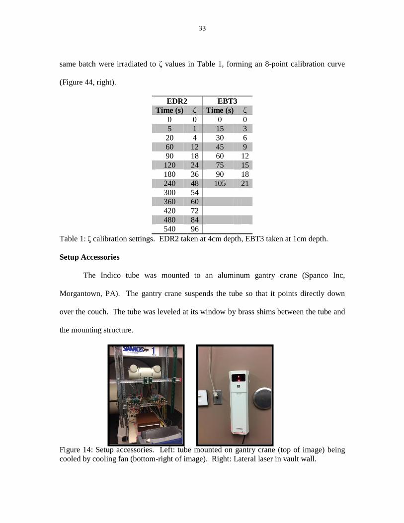
same batch were irradiated to ζ values in Table 1, forming an 8-point calibration curve

(Figure 44, right).

EDR2 EBT3

Time (s) ζ Time (s) ζ

0 0 0 0

5 1 15 3

20 4 30 6

60 12 45 9

90 18 60 12

120 24 75 15

180 36 90 18

240 48 105 21

300 54

360 60

420 72

480 84

540 96

Table 1: ζ calibration settings. EDR2 taken at 4cm depth, EBT3 taken at 1cm depth.

Setup Accessories

The Indico tube was mounted to an aluminum gantry crane (Spanco Inc,

Morgantown, PA). The gantry crane suspends the tube so that it points directly down

over the couch. The tube was leveled at its window by brass shims between the tube and

the mounting structure.

Figure 14: Setup accessories. Left: tube mounted on gantry crane (top of image) being

cooled by cooling fan (bottom-right of image). Right: Lateral laser in vault wall.

34

A second independent mounting structure was hung from the gantry crane to

support the MLC. Commissioning of the beam required aligning the MLC to the center

of the beam, which was performed experimentally (see Chapter 5).

A laser alignment system is necessary to align the phantom with isocenter before

and during treatment. A lateral laser was mounted into the wall of the cyclotron room,

and a longitudinal laser was held in place by magnetic supports on the MLC support

structure. A vertical laser exists, but was not necessary because the couch was kept static

throughout each treatment. Vertical distances were measured using a tape measure from

the point of interest to the source position on the x-ray tube, as indicated by a sticker and

adjusted relative to the vertical laser. The MLC was placed, taking advantage of the laser

system, halfway between the beam and the target.

Flattening Filter Design and Superficial Compensators

The flattening filter for the Indico tube was created as part of a study to create 3D

printed superficial compensators for kilovoltage tubes. This study will be detailed in

Chapter 5. The filter is located in a 3D-printed jig along with a 0.156mm tungsten disc at

the beam aperture (Figure 10, right).

35

CHAPTER 4 THE BRASS MULTI-LEAF COLLIMATOR

This chapter discusses computer-aided metalworking, the original brass multi-leaf

collimator design and creation, the errors that arose, and how their severity necessitated a

redesign of the MLC.

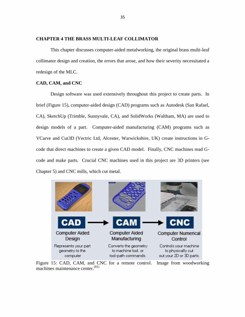
CAD, CAM, and CNC

Design software was used extensively throughout this project to create parts. In

brief (Figure 15), computer-aided design (CAD) programs such as Autodesk (San Rafael,

CA), SketchUp (Trimble, Sunnyvale, CA), and SolidWorks (Waltham, MA) are used to

design models of a part. Computer-aided manufacturing (CAM) programs such as

VCarve and Cut3D (Vectric Ltd, Alcester, Warwickshire, UK) create instructions in G-

code that direct machines to create a given CAD model. Finally, CNC machines read G-

code and make parts. Crucial CNC machines used in this project are 3D printers (see

Chapter 5) and CNC mills, which cut metal.

Figure 15: CAD, CAM, and CNC for a remote control. Image from woodworking

machines maintenance center.(81)

36

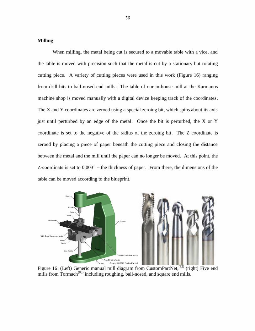
Milling

When milling, the metal being cut is secured to a movable table with a vice, and

the table is moved with precision such that the metal is cut by a stationary but rotating

cutting piece. A variety of cutting pieces were used in this work (Figure 16) ranging

from drill bits to ball-nosed end mills. The table of our in-house mill at the Karmanos

machine shop is moved manually with a digital device keeping track of the coordinates.

The X and Y coordinates are zeroed using a special zeroing bit, which spins about its axis

just until perturbed by an edge of the metal. Once the bit is perturbed, the X or Y

coordinate is set to the negative of the radius of the zeroing bit. The Z coordinate is

zeroed by placing a piece of paper beneath the cutting piece and closing the distance

between the metal and the mill until the paper can no longer be moved. At this point, the

Z-coordinate is set to 0.003” – the thickness of paper. From there, the dimensions of the

table can be moved according to the blueprint.

Figure 16: (Left) Generic manual mill diagram from CustomPartNet,

(82) (right) Five end

mills from Tormach(83)

including roughing, ball-nosed, and square end mills.

37

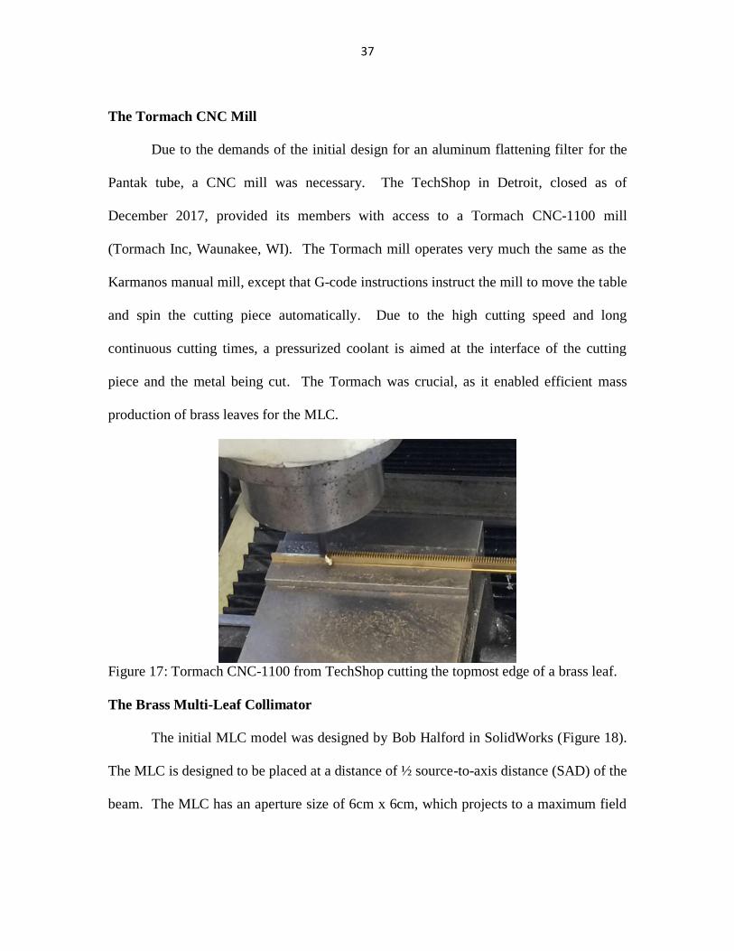
The Tormach CNC Mill

Due to the demands of the initial design for an aluminum flattening filter for the

Pantak tube, a CNC mill was necessary. The TechShop in Detroit, closed as of

December 2017, provided its members with access to a Tormach CNC-1100 mill

(Tormach Inc, Waunakee, WI). The Tormach mill operates very much the same as the

Karmanos manual mill, except that G-code instructions instruct the mill to move the table

and spin the cutting piece automatically. Due to the high cutting speed and long

continuous cutting times, a pressurized coolant is aimed at the interface of the cutting

piece and the metal being cut. The Tormach was crucial, as it enabled efficient mass

production of brass leaves for the MLC.

Figure 17: Tormach CNC-1100 from TechShop cutting the topmost edge of a brass leaf.

The Brass Multi-Leaf Collimator

The initial MLC model was designed by Bob Halford in SolidWorks (Figure 18).

The MLC is designed to be placed at a distance of ½ source-to-axis distance (SAD) of the

beam. The MLC has an aperture size of 6cm x 6cm, which projects to a maximum field

38

size of 12cm x 12cm at isocenter. The design contains 24 brass leaves in each of two

banks for a total of 48 leaves. Leaves are moved using powered gears in gear rack that is

milled directly into the leaves. The gears are spun about a rod by a stepper motor and

gear assembly, which is held in place between a two-sheet frame with brass bearings.

The gears and steel rods act to hold the leaves in place at their contact point, regardless of

MLC orientation. The stepper motors are controlled (Chapter 6) by an Arduino assembly

driven by a custom graphical user interface (GUI). The vast majority of this design was

kept for the MRC that would be built, and further details will be described in the MRC

section below. The brass leaves, however, did not make it through to the final design.

Figure 18: Initial model of MLC in Solidworks.

39

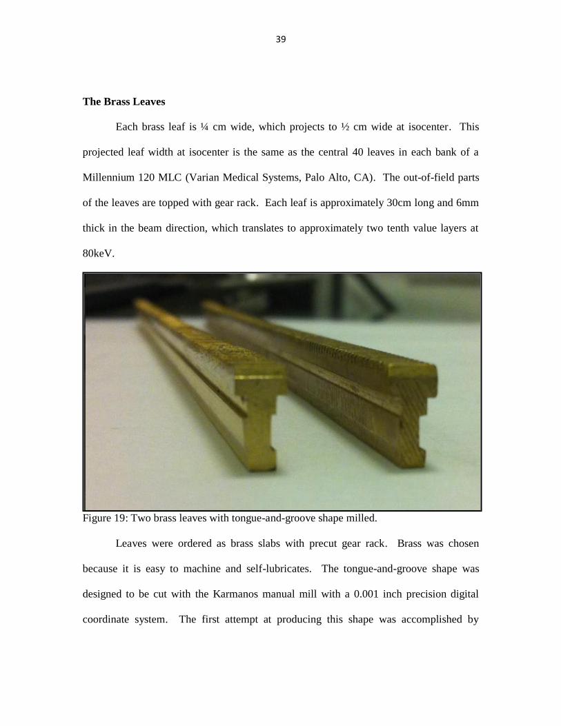
The Brass Leaves

Each brass leaf is ¼ cm wide, which projects to ½ cm wide at isocenter. This

projected leaf width at isocenter is the same as the central 40 leaves in each bank of a

Millennium 120 MLC (Varian Medical Systems, Palo Alto, CA). The out-of-field parts

of the leaves are topped with gear rack. Each leaf is approximately 30cm long and 6mm

thick in the beam direction, which translates to approximately two tenth value layers at

80keV.

Figure 19: Two brass leaves with tongue-and-groove shape milled.

Leaves were ordered as brass slabs with precut gear rack. Brass was chosen

because it is easy to machine and self-lubricates. The tongue-and-groove shape was

designed to be cut with the Karmanos manual mill with a 0.001 inch precision digital

coordinate system. The first attempt at producing this shape was accomplished by

40

Mayville(84)

and Koh. Six cuts and three end mill sizes were required. Mayville(84)

milled a steel jig to aid in fastening the leaf in place for cutting.

Equipment used for production of the 48 brass leaves included Cut3D CAM

software and the Tormach CNC mill. Cut3D was used to learn G-code basics. The G-

code produced from Cut3D was then hand-modified to create four toolpath scripts for the

brass leaves – one for the tongue side, one for the groove side (each with a 1/8” steel

square end mill), one for the groove itself (with a smaller 5/32” steel square end mill),

and one final cut (with the 1/4” tungsten carbide square end mill) for gear rack removal

of the portion of the leaf that would collimate the beam. All 48 brass leaves were cut

using this method to tolerance.

HVL and Penumbra Testing

An experiment was performed to determine whether the penumbra and HVL of

the brass were sufficient to attenuate the Pantak beam. Leaves were placed into the MLC

assembly and mounted to the Pantak tube. EDR2 film was irradiated in four situations:

MLC open so one edge was isocentric, and MLC open more than isocentric, completely

closed MLC, and an open field shot with the MLC removed. The first two scans tested

penumbra for our rectangular edges due to unfocused design. The final two scans tested

transmission and interleaf leakage. All four experiments were set to 120 kVp and 10 mA

for two minutes.

41

Figure 20: Brass leaf penumbra measurements, taken at and off isocenter.

(85)

Transmission and interleaf leakage were found to be zero. Interleaf leakage is

faintly visible on film, but undetected by our film scanner despite 71 DPI spatial

resolution. Penumbra at isocenter was found to be 0.72mm, which matched the

penumbras of true field edges. Penumbra off-isocenter was 1.1mm.

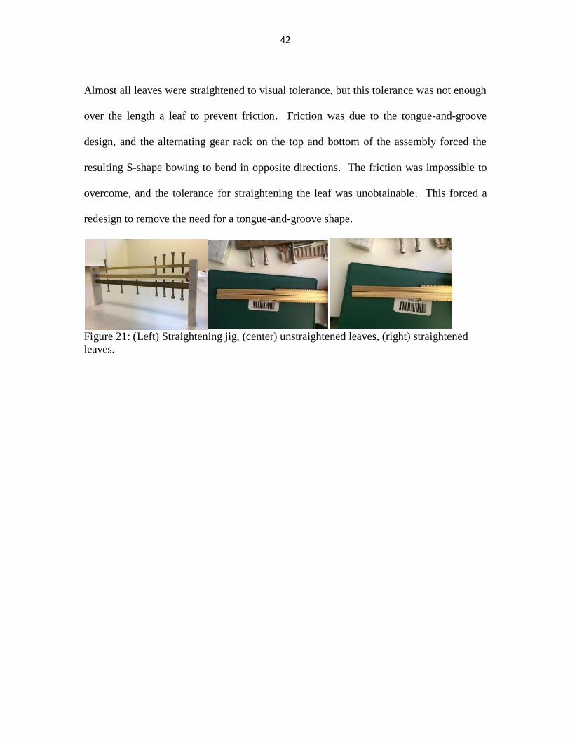
Need for Redesign

Substantial bowing was expected in the cut brass. The invaluable steel jig from

Mayville was created specifically to minimize bowing during the cutting process. A

bowing in the X-Y direction was easy to flex out physically due to the long and thin

shape of the leaves. Bowing in the Z direction, however, could not be fixed by hand. All

leaves were placed on a perfectly-flat stone (or “surface plate”) under heavy weight for

one month to remove bowing. This was not sufficient.

A four-piece straightening jig (Figure 21) was designed and fabricated using the

Tormach CNC mill, a tap, and Autodesk CAD software at TechShop. The jig was

capable of receiving a leaf and straightening it at several pressure points using screws.

42

Almost all leaves were straightened to visual tolerance, but this tolerance was not enough

over the length a leaf to prevent friction. Friction was due to the tongue-and-groove

design, and the alternating gear rack on the top and bottom of the assembly forced the

resulting S-shape bowing to bend in opposite directions. The friction was impossible to

overcome, and the tolerance for straightening the leaf was unobtainable. This forced a

redesign to remove the need for a tongue-and-groove shape.

Figure 21: (Left) Straightening jig, (center) unstraightened leaves, (right) straightened

leaves.

43

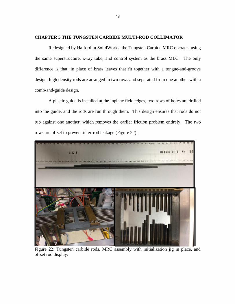
CHAPTER 5 THE TUNGSTEN CARBIDE MULTI-ROD COLLIMATOR

Redesigned by Halford in SolidWorks, the Tungsten Carbide MRC operates using

the same superstructure, x-ray tube, and control system as the brass MLC. The only

difference is that, in place of brass leaves that fit together with a tongue-and-groove

design, high density rods are arranged in two rows and separated from one another with a

comb-and-guide design.

A plastic guide is installed at the inplane field edges, two rows of holes are drilled

into the guide, and the rods are run through them. This design ensures that rods do not

rub against one another, which removes the earlier friction problem entirely. The two

rows are offset to prevent inter-rod leakage (Figure 22).

Figure 22: Tungsten carbide rods, MRC assembly with initialization jig in place, and

offset rod display.

44

Plastic gear rack was created separately and glued to the rods with two-part

epoxy. A plastic comb was required for each bank to serve three purposes: to keep the

gear rack aligned with the rods, to prevent friction between the gear rack of adjacent

leaves, and to provide sufficient force to oppose pressure from the gears. Rods needed to

be cut to a position-specific size to accommodate this design.

3D Printing

Three plastic pieces were briefly described above: comb, guide, and gear rack.

Each of these designs could have been ordered online or fabricated from spare plastic in

the department, but this would have been at great expense or would require precise mass

manufacturing skills. Instead, an investment was made in a 3D printer, which also

permitted manufacturing of other parts and opens significant research and prototyping

potential. There are many kinds of 3D printers that print everything from plastic trumpet

mouthpieces to concrete and steel skyscrapers.(86)

This section will only consider the

fused deposition modeling (FDM) technique.

FDM 3D printing requires a long string of cold filament material to be forced

through a hot end, which is a heated nozzle. The tip of the hot end is precisely placed in

the X-Y plane parallel to the ground.(87)

The filament melts in the hot end and is extruded

as a molten smear onto a bed, which is a sheet of glass about the size of a piece of paper.

This bed heats up to better adhere to the molten material, which is smeared in a thin layer

and quickly cools. The bed then moves downward in the Z direction and a new layer is

printed upon the old layer. This process repeats over and over again until the part is

45

created in a desired shape. The most typical filaments in FDM 3D printing are ABS

(acrylonitrile butadiene styrene) and PLA (polylactic acid).

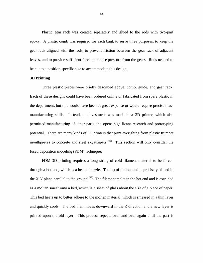
Airwolf 3D HD2x

Our group invested in an Airwolf 3D (Fountain Valley, CA) HDx for this project.

The device was later upgraded to an HD2x through firmware and the addition of a dual

nozzle mechanism. The HD2x is capable of producing a part with a slice area of 30cm x

30cm and a height of 20cm in layers 0.1mm thick (fine resolution) through 0.3mm thick

(coarse resolution) using two materials simultaneously. The included hot end nozzles

have a 0.5mm diameter, which was upgraded to a finer diameter of 0.35mm. The hot end

and glass bed move with submillimeter accuracy using stepper motors. After a slice is

complete, the glass bed shifts down by one slice thickness and the next slice begins. The

first slice of a part is unique in that it is 0.4mm thick and difficult to adhere to the hot

glass.

The HD2x operates with MatterControl (MatterHackers, Foothill Ranch, CA)

CAM control software that translates any model in the stereolithography (.stl) file format

into G-code for printer layers. CAD models for the guide, comb, and gear rack were

created in SolidWorks. All other models were drawn in SketchUp.

46

Figure 23: Airwolf 3D HD2x FDM 3D Printer.

We found that PLA plastic properly adheres to the bed if the bed is kept at 40ºC

and layered with 3M (Maplewood, MN) blue painter masking tape. PLA printed best

with a hot end temperature of 220ºC. This technique was used for all printed parts.

Our printer was used to print gear rack, comb halves, rod guides, mounts for the

circuitry, and a flattening filter for the beam. Flattening filter design was a subject of

intense study and will be saved for its own section farther below. The other parts are

described here:

Gear Rack

Gear rack was printed on its side with the 0.35mm nozzle to enhance resolution of

the rack teeth. All racks were identical regardless of rod position in the MRC. Racks

measured 0.3cm x 0.3cm x 10cm, with a divot on the bottom side 2cm from an edge to

aid in the adhesion of a tungsten carbide rod to the proper location. There are 64 teeth on

47

each rack. In one instance, due to milling errors, a gear was positioned too high for its

rack to reach. This was fixed by printing a rack with an additional 3mm of thickness.

Figure 24: Gear rack, with gear and rod.

Comb

Two combs (Figure 25) were printed to provide each gear rack its own dedicated

track. As stated above, the comb keeps the gear racks aligned with the rods, prevents

rubbing between adjacent gear racks, and acts as a pressure point to oppose the gears.

Because 3D printed parts require a flat surface to adhere to the printing bed, the combs

were printed in two halves and attached with two-part epoxy. The combs were held in

place in the frame by four thin metal rods each, requiring holes to be drilled into the

frame and combs.

A slight rotation of one comb is blamed for a load issue on two particular leaves

in the MRC. One rack of one leaf was found to be so far from its gear that a new gear

rack had to be printed at a larger height. A second gear is so pressed into its gear rack

that the gear cannot turn without hand-motion.

48

Figure 25: Comb, fully assembled.

Rod Guide

A rod guide (Figure 26) was printed as an entry point for each carriage. When the

leaves are parked, the tips of the leaves are flush with the field side of the rod guide. The

printed guides included pilot holes. These holes, due to the layering nature of the

printing process, were not perfectly round and needed to be drilled out. Additional holes

and surfaces are used to fasten the guide to the steel frame.

49

Figure 26: Rod guide, as rendered by 3D Paint CAD (Microsoft Corp, Redmond, WA)

Circuitry Mounts

Four large green circuit boards distribute power to move the leaves. These boards

needed to be suspended within the cable length of the motors, out of the field, and had to

move with the device. The solution was to mount them to the outside of the exterior

motors. Brackets were designed and printed to hold the circuit boards in place with

screws. Holes were tapped into the steel frame approximately 60mm apart to align with

the holes present in the circuit board. The brackets hook on the bottom of the boards to

permit removal and attachment of stepper motor connections with appropriate force. The

brackets were printed on coarse (.3mm/layer) resolution as described above. The use of a

flat edge on the sides allowed for fast, easy printing. A jig was also designed to hold the

microcontroller board (Chapter 6) above some of the motors. This design takes

advantage of existing screws that hold the motors to the frame and repurposes them to

also hold this jig in place.

50

Figure 27: Microcontroller jig (left) and circuitry mount (right), as modeled in SketchUp.

Superficial Compensators

The 3D printer was also used to create the plastic flattening filter using a script

written in MATLAB to create compensators for superficial beams.(88)

The necessary

inputs for this script are the HVL of the plastic filament for the incident beam energy, the

contour for which compensation is necessary, and an origin point within the model. The

contour is exported from a TPS in DICOM-CT, smoothed, simplified, and converted into

.stl format using open-source software. In .stl, a vertex maps each point on the patient

surface from an origin point. Our in-house MATLAB package normalizes this map to

originate at the tube focal spot and transforms each vertex as a ray length through the

initial fluence function. Adjusted rays are modeled through exponential attenuation in a

user-selected material to achieve uniform surface fluence. Calculated material thickness

for each ray is projected to a flat plane at a predetermined distance from the source,

which forms a 3D-printable model of a compensator.

This workflow was tested on a 3D-printed breast scar phantom using PLA and the

Indico 100. The phantom was irradiated for a set mAs with and without a compensator,

taping OSLDs to the surface at eight locations for each measurement. These readings

51

were used to calculate relative deviation from the central OSLD. OSLD measurements

demonstrate that the compensator substantially improves dose deviations across the part

contour. Crossplane maximum deviations improved from 17% to 2.0%, while inplane

and diagonal deviations improved from over 25% each to approximately 10% each. This

is due to the heel effect

Briefly, the heel effect occurs as a consequence of the design of a reflection x-ray

tube (Chapter 3). Many of the x-rays produced in the anode are attenuated within the

anode itself. This results in decreased intensity on the anode side of the field in the

inplane direction. The inplane direction is much more difficult to compensate, and the

shape of a compensator or flattening filter must take this into account.

Flattening Filter

A flattening filter can be defined as a compensator for a flat surface at a chosen

depth. Flattening filters in MV beams are considered successful if they produce a flat

dose distribution at 10cm depth in a cube of water with its surface at isocenter. Our

Monte Carlo model assumed a flat isodose distribution at the surface of a phantom placed

at isocenter. The superficial compensator work was directly applied to the kV beam to

create its flattening filter by assuming a flat surface at 60cm.

Tungsten Carbide Rods

The since-decommissioned neutron cyclotron at the Karmanos Cancer Center was

equipped with a large multi-rod collimator made from many 1/8” diameter, 272mm long

tungsten carbide rods (Figure 22, above). While intended for neutrons, the diameter of

52

these rods is over 2 TVLs for 80keV photons. This makes them an excellent choice for

collimating our kV beam.

Rods left over from the former MRC were repurposed in this work, but needed to

be cut to size. Six different sizes were required: 100, 117, 142, 157, 185, and 203mm. A

set of all six lengths could be cut from four 272mm rods. This task required a diamond-

coated angle grinder due to the hardness of tungsten carbide (Figure 28). Once cut, all

rod sizes were finely tuned with a disk sander.

Figure 28: Rod sizing process. (Left) rod in vice. (Right) diamond tipped angle grinder.

Once the leaves were the correct shape, they were notched to gear rack and sealed

in place using two-part epoxy. The dried epoxy was then trimmed with a razor to prevent

unnecessary friction with nearby leaves. Finally, the completed rods were inserted into

the comb-and-guide assembly within the frame, gears and steel rods were assembled to

hold the gear rack in place, and the entire MRC device was mounted to the

superstructure.

53

Issues with the MRC

Many difficulties were encountered while testing the MRC. The two-part epoxy

was difficult to trim down to the point where the leaves would not contact one another.

Due to the point of insertion with the original neutron device, some rods had an irregular

end. Whenever possible, these were kept out of the field and instead glued to the gear

rack. Leaf ends were lubricated with white lithium grease to help with friction in the rod

guide, the holes of which needed to be drilled out further than designed. Due to

continuing issues with the rods in the rod guide, the “Park” command in the Qt GUI

withdraws leaves to 5mm from the field edge so a leaf is never fully retracted. It is for

this reason that the relative time index ζ for EBT3 is defined with the field in this position

(Chapter 3). Finally, the .mlc files required editing to account for an interdigitation flaw

(Chapter 6).

More pressing issues involved the control system (Chapter 6). One carriage

performed admirably throughout the process, but the other carriage had some leaves

under too high or too low of a physical load. This may have been due to the comb being

slightly improperly drilled when placed into the frame, but troubleshooting this issue

would have required disassembling the entire device. Issues with load were partially

resolved with the printing of a larger piece of gear rack for one rod, but the remaining

load necessitated placing the faulty carriage closer to the microcontroller along the circuit

as outlined in Chapter 6. The phantom irradiation was treated with this flip in mind, as it

required reorienting the coordinate system so that the foot of the couch became the head

of the patient (as pictured in Figure 42, left).

54

Once the MRC worked, there were minor flaws in the design that required the

creation of pseudo-jaws. Due to the two-level effect of the rod guide, the rods on each

level project slightly different widths on the phantom (Figure 29). While this impact is

minimal, the projection of the far exterior rods is not sufficient to cover the very edge of

the field. As a result, there are lines of fine leakage on the longitudinal edges where Y

jaws would normally be on a Varian device. Also due to the absence of Y jaws, the rod

closure points cause interleaf leakage that must be covered. A set of pseudo-jaws was

created from several layers of lead sheet taped together and carefully placed over the gaps

before each field. A pair of tungsten carbide rods that were considered waste from the

cutting process were cut to size and inserted on the fine field edges so they were

permanently covered.

To extend the life of the power supplies, they were turned off after each leaf

motion and only turned on just before launching the Qt software. This slowed down the

delivery of IMRT fields, but erratic behavior of the Qt software was not an issue from

this point forward. This is likely because the software was restarted after each use.

55

Figure 29: EDR2 alignment image, with rods exposed at random. Fine leakage is seen at the bottom right and top left.

56

CHAPTER 6: MLC CONTROL SYSTEM

The MLC is controlled by in-house software and custom-printed circuitry. This

chapter details the flow of control from the shaping command (in the form of a .mlc file,

as exported from Eclipse), to the turn of the motors that drive the leaves to make the

desired shape (Figure 30). Much of this is done by a control application written in Qt

(Santa Clara, CA) by Snyder. It is easiest to describe this process starting with the

motors and moving back along the control system signal pathway to its origin as a .mlc

file.

Figure 30: Diagram of MLC control system. Data originates as .mlc, imported into Qt,

translated into Arduino commands, into Arduino microcontroller, converted into binary

switch commands to appropriately power motors. Motors are connected in serial, but

powered in parallel via shift registers and Darlington arrays.

57

Figure 31: Stepper motor with gear attached, with five wires (bottom).

Stepper Motor

Each leaf is controlled by a stepper motor (Figure 31), model number 28BYJ-48,

5V DC. There are five wires on each motor: one (red) goes to +5V and links in parallel

to four coils, and the other four wires individually reach the opposite end of the four

coils. By grounding the four coils in sequence (Figure 32), the motor will be rotated.

The sequence shown below is the “half step” sequence, which pushes the motor half of a

step per change of signal. A “full step” sequence would leave out the odd-numbered

steps, reducing the time required but also reducing the accuracy of the motor. Our

system uses the full-step method, which does not include half-steps 1, 3, 5, or 7 below. A

single step rotates the motor 1/64 of its rotation, but an internal gear train translates this

into 1/63.68395 turns of the gear.(89)

A full rotation of the gear requires 2038 steps.

58

Figure 32: Stepper motor connected to Darlington Array board; circuit diagram showing

4 coils and +5V wire opposite coils from wires 1-4; half-step sequence, with each half-

step in a column and each participating coil in a row. Image from 42bots.com(89)

To ground the four wires in sequence, an accurate signal must be sent. The code

for such a signal is simple: send 0001; 0011; 0010; 0110; 0100; 1100; 1000; 1001 in

order to get the switching sequence in Figure 32. An important issue is that this sequence

must be sent with enough energy to actually turn the motor. The Arduino UNO board,

powered by a USB cable from a laptop, cannot power a single motor without an

amplifier.

Darlington Array

A Darlington Array is a set of seven pairs of bipolar transistors (Figure 33, left).

Transistors are used to amplify electronic power or switch signal on and off. The motor

will draw the necessary current through the Darlington Array switch when thrown. The

array further provides suppression diodes that prevent back EMF after switch-off of coils.

59

A Darlington Array board designed to connect to a stepper motor is shown below

(Figure 33, right). A transistor pair is used for each of the four coils, so the four

corresponding wires from the motor are hooked up to output pins of their respective

transistor. The GND and COM pins (“DC Power,” below) are connected to ground and

the 5V power supply voltage, respectively. The commands to ground each wire, driving

the motor, are sent through the input terminals (“Signal from micro-controller”) as

binary, following the half-step switching pattern above.

Figure 33: (Left) Darlington transistor schematic. (Right) close-up of sample Darlington

Array board. Stepper motor connector takes in the five wires from the stepper motor.

Signal from micro-controller accepts input commands for the four wires. The +5V wire

is connected to DC Power. The array switches the power on and off to different coils to

turn the motor. Images from 42bots.com(89)

Even with Darlington Arrays amplifying the signal of the input chip, a laptop

using an Arduino controller can only power two stepper motors. A solution to this

problem is to hook up 48 motors to 24 USB cables and 24 Arduino chips, powering them

through a tower with 24 USB ports. A better solution is to use shift registers.

60

Shift Register

Shift registers are necessary to control 48 motors with one laptop, one Arduino

controller, and one USB cable. A shift register is effectively an 8-bit storage unit that

starts as eight zeroes. Given an incoming DATA signal from the microcontroller (a 0 or

a 1), at a periodic CLOCK signal the shift register will check for the incoming 0 or 1.

Once checked for, the 0 or 1 is always saved in bit “1” of the 8 bits. The clock signal is

then sent again, and as a new 0 or 1 is saved in bit “1” of the 8 bits, that original value is

shifted to bit “2”. When another new bit is checked and saved in bit “1”, bit “2” sends its

value to bit “3”, bit “1” sends its old value to bit “2”, and so on. This enables the shift

register to be filled by a single serial source as the old data is shifted downstream.

Figure 34: A 4-bit shift register diagram, from Aspencore,(90)

showing shift of binary

signal. Binary serial DATA signal enters from the left. Incoming CLOCK and LATCH

signals enter from parallel input (bottom). CLOCK signals instruct all bits to accept data

from the left. LATCH signals instruct all bits to send their current data through parallel

output (top). All three signals (DATA, CLOCK, LATCH) originate in the Arduino

board.

It is possible to connect shift registers in series. By doing so, a shift of the old

data will continue on to the next shift register. By extension, if 24 shift registers were

61

connected in series, then only the first bit of the first shift register would be filled by

incoming data. That data could then shift all the way down the chain to the final bit of

the 24th shift register after 192 CLOCK signals. So, data for the last shift register in a

chain can be sent early and shifted down until all 24 shift registers are filled with a

deliberate combination of zeroes and ones.

Once filled appropriately, the series of shift registers is sent a signal called

LATCH, which commands the shift register to send its stored data simultaneously

through its eight output pins. These pins, for our circuit, are connected to Darlington

Arrays. Since there are eight shift register outputs and only four required Darlington

inputs per motor, each shift register connects to two Darlington Arrays. The signal for a

single shift register could be 10011001, which would command both of the attached

motors to continue a half-step from, say, half-step 7 to half-step 8 in Figure 32. This

command drives the leaves 1/4076 of the circumference of the gear and takes about

0.5ms.

The 16 pins of a shift register include eight output pins, one pin each for incoming

and outgoing data, one pin each for 5V and GND, a pin for LATCH, a pin for CLOCK,

and two pins that are not used in this project.

62

Figure 35: (Left) 74HC595 shift register schematic from Texas Instruments.(91)

Output

pins labeled QA-QH, 5V pin labeled VCC, clock pin labeled SRCLK, and latch pin

labeled OE. (Right) A shift register (top black rectangle) feeding two Darlington arrays

(bottom two black boxes) which feed stepper motor wires.

Circuit Board

The circuitry, designed by Snyder and soldered by Koh,(92)

daisy chains 24 shift

registers in serial fashion to send signals to 48 Darlington arrays in parallel that in turn

amplify signal to power 48 stepper motors simultaneously. This is accomplished across

four boards, each connected in parallel to power supplies with three wires: one is ground

and two are +5V. The two +5V wires power the stepper motor system and the Darlington

array / shift register system, respectively. This setup separates the control system and

motor power draws to reduce noise. The boards are connected to one another in serial

with three wires – one for each shift register function of DATA, CLOCK, and LATCH.

These three serial wires connect to the Arduino microcontroller output pins, which are the

signal starting point. The first batch of data sent is the data for Motor 48, which is the

farthest motor away through the wires. This will move Leaf 48 in the top-left of the

MLC. The final batch is the data for Motor 1, which is closest to the signal and moves

Leaf 1 in the bottom-right.

63

The boards are connected to one another through copper wire. An Ethernet CAT5

cable contains four pairs of copper wires that run the length of the cable. The ends of

CAT5 cables were cut and crimped to connectors for our circuit boards. As just

described, three wires were connected in serial from one board to another, while three

wires were connected directly from a board to the power supplies. (Figure 36)

Figure 36: diagram of wiring for circuit boards. 12 motors (orange), powered by 12

Darlington arrays (black), commanded by 6 shift registers (blue), which operate on three

signals. The signals originate in the Arduino board. CAT 5 cables provide power to the

boards and link the shift registers across boards.

The serial-signal to parallel-motion process is slower than desired for many

robotic functions using stepper motors, but for the purpose of this work it is more than

adequate. The leaves can traverse our 6cm aperture in fewer than 15 seconds, which is

the same order of magnitude as commercial MLCs.

Arduino Microcontroller

The output signals sent through the Data, Clock, and Latch wires are controlled

by an Arduino UNO microcontroller board. The microcontroller contains firmware that

converts incoming commands from a USB cable into timed binary commands for Data,

Clock, and Latch as described above. The Arduino UNO is pinged at the beginning of

each session and instructed to await commands. Commands are sent as a string of the

64

number of steps for each motor, separated by colons and followed by a colon and an

asterisk, which signals the Arduino that the string has terminated and to initiate motions.

Conversion of this string into timed signals is governed by custom firmware.

Figure 37: (Left) Arduino UNO microcontroller attached to MLC. (Right) Pin

connection to board, wires from the front are data, latch, clock.

Qt software

The Arduino board receives a signal from an in-house GUI and command

software created using the Qt software suite. The GUI contains functionality to test

communication with the Arduino board. Though there is no secondary check, the

software does prevent motion that would cause leaves to come in contact with one

another. The software can be used to move any leaf or leaves to any position, and

contains initialization, parking, and .mlc file loading capabilities.

To initialize the MLC, a 3D-printed plastic jig is inserted into the frame snugly

such that a 1.0cm-thick block is in the path of all leaves and centered along the central

axis (Figure 38). After leaves are moved to make contact with the block, the

65

initialization function saves all positions as 0.5mm or -0.5mm, depending on carriage.

This effectively zeroes the leaves.

Figure 38: Initialized MLC. Leaves are manually set to touch the edges of a 1cm-thick

plastic jig. The GUI then knows the absolute location of each leaf and can send relative

commands.

The GUI can be used to load field shapes in the format exported from Eclipse

(.mlc) after conversion to .d00 in a text editor. To load a .d00 file, the software calculates

the displacement between the current location of the leaves and the destination of the

leaves. If leaf motion is necessary, the software calculates the number of millimeters that

each leaf must be moved and the necessary direction. The number of millimeters is

translated into the appropriate number of steps using the known diameter of the gear, and

commands are then sent to the microcontroller to turn the motors. Due to the position of

the MLC at ½ SAD, actual motion of the leaves is ½ the motion of the field projected at

isocenter in .d00 files.

66

Figure 39: GUI in Qt

To summarize the entire process: a laptop with Qt is plugged via USB into an

Arduino UNO board. The board is pinged, and a .d00 file is loaded into the software.

The software calculates the number of steps and direction necessary to move each leaf

from its current position to the desired position, and these are sent as positive or negative

integers separated by colons in a string to Arduino. Arduino then converts these into a

timed set of DATA and CLOCK signals that are sent through 24 shift registers connected

in serial. At the conclusion of each step, a LATCH signal is sent that sends the DATA in

parallel out through Darlington Arrays and into Stepper Motors. The motors then move

the leaves. When the appropriate number of steps is run, the Arduino stands by. The GUI

updates its files with the current leaf position and also stands by.

67

Figure 40: Qt software running to MLC.

Power Supply

The entire control system functions with +5V power. This voltage must remain

constant. A pair of +5V/4A power supplies were connected in parallel in constant

voltage mode. This permitted a maximum power draw of 8A. The motors each have 42

Ohms of resistance, so at 5V this requires about 5.7A. Power also needed to be supplied

to the shift registers, Darlington arrays, and the Arduino microcontroller, and the motors

needed to operate under load.

68

Figure 41: BK Precision power supplies, connected in parallel and run through CAT5

cables.

Control System Commissioning

After initial assembly, a few things became apparent immediately. The most

apparent was that the leaves were moving in seemingly random directions when asked to

move in one direction. This was because leaf motion in and out of the field was

interpreted as being clockwise and counterclockwise rotation of the motor, respectively.

The MLC design flips some motors to conserve space, so an “in” command would pull

half of the leaves out. The design was such that every fourth leaf moved correctly or

incorrectly. A gate was created in the code to check for the position of the leaf and

multiply its motion by -1 if it was moving incorrectly.

The motion of the leaf was originally assumed to be one diameter of the gear per

rotation instead of one circumference, so the distances needed to be divided by pi.

Furthermore, the typical use of a .d00 file is such that saved data are the positions of the

leaves projected at isocenter. Thus, a position of 1cm would require the leaf to be at a

position of 0.5cm in our situation. All ordered leaf motions were cut in half and the

69

initialization and park codes were adjusted accordingly. Other than these very minor

issues, the Qt software worked as designed.

Circuitry Issues and Fixes

Capacitors were wired in the circuit boards to minimize noise. Several capacitors

were lost over the course of this project and needed to be replaced and soldered. Some

wires required crimping to new connectors after these were pulled out by accidental

tugging on the wires. One faulty motor required replacing, but otherwise the circuitry

performed admirably. No Darlington Array or shift register replacements were

necessary. Due to load issues, the right-side carriage of leaves was harder to move. The

connections were adjusted to make the right-side carriage closer to the initial signal,

which cleared up this issue to the point where only severe load problems caused motor

issues.

One power supply was lost over the course of this work. This happened after the

parallel connection between the negative terminals of the two supplies was accidentally

severed. In order for current to reach ground in the top supply, it had to flow through the

bottom supply. This resulted in a burnt-out bottom supply. Luckily, a replacement was

on site that lasted the duration of the experiment.

An issue that is left unresolved is mechanical. Stepper motors have a small

amount of play when reversing direction. This caused issues during IMRT deliveries, in

that after four fields worth of delivery the leaves needed to be reinitialized about 2mm to

the left, with respect to the field. Leaf position is therefore estimated to have

submillimeter precision just after initialization, growing to +- 2mm uncertainty after four

70

IMRT fields. Leaves were visually inspected prior to each delivery for obvious errors,

such as those that arose due to interdigitation problems.

71

CHAPTER 7 PHANTOMS AND TREATMENT PLANNING

This chapter details the input data and output devices of kIMR. Specifically, it

details the phantoms that were irradiated by the modality, the materials used by these

devices to measure relative dose, and the treatment planning system used to calculate and

create MLC shapes and delivery time for each field.

Phantoms

For simplicity, the kIMR prototype was designed to not require a gantry or rotate

about a phantom. Instead, the phantoms were positioned with their target at isocenter and

rotated to simulate a rotating gantry. Phantoms were required to have a slot for film to

provide relative depth dose measurements. Five phantoms were used over the course of

this work to calibrate the modality and determine dose falloff properties.

Figure 42: Head phantoms used for our study, from left to right: Lucy, Rando, Max-HD

Lucy

The Lucy phantom (Standard Imaging, Middleton, WI) is a 7cm radius Lucite

sphere (Figure 42, left) that is designed for stereotactic radiosurgery QA. The device

functions with modular inserts, including a single BB insert at the center of the sphere

72

and a radiochromic film insert that pricks a small square of film twice in one corner for

alignment and once in the other three corners. The Lucite sphere can be aligned to rotate

about the coronal and axial planes, and an angle indicator with 5-degree intervals is

clearly marked on its stand. The stand suspends the center of Lucy about 18cm above the

couchtop.

Rando

The Alderson(93)

Rando phantom (Radiology Support Devices, Long Beach, CA)

is a real human skeleton encased in a mold of solid water, with lower density plastic in

the lungs. The skeleton and plastic mold is sliced into many axial slabs, which permits

custom-cut radiochromic film to be placed between slabs in order to measure depth dose

characteristics in an anatomically accurate heterogeneous subject. Rando phantoms are

commonplace in medical physics and have even been sent to outer space for various

experiments.(94)

The head of the KCI Rando phantom was used to provide anthropomorphic,

heterogeneous measurements to determine the effect of the skull. The top three slabs of

the head were viced in a MedTec (Orange City, IA) MT-DS-2000 IMRT phantom

(Figure 42, center). A wooden disc at the top of the Rando head was used to align the

phantom at the correct angle against a 360-degree protractor printed at the size of the disc

and attached to the solid water. The center of this protractor was taped at the vertical and

lateral location of the isocenter, and the longitudinal location was placed between slabs 2

and 3 (laser in Figure 42, center). Radiochromic film was custom-cut with a paper cutter

to fit between these slabs, and holes were carefully punched at dowel pin locations.

73

Max-HD

The IMT Max-HD head-and-neck phantom(95)

was originally set to be used in this

experiment for 3D conformal and IMRT deliveries, but it could not be reproducibly

rotated about isocenter. The phantom contains an axial dose plane in its brain, along with

several OSLD and ion chamber locations in the neck region. The phantom is

anthropomorphic and heterogeneous (Figure 42, right) due to proprietary anatomically

accurate plastic composition. The Max-HD was irradiated with a single field in order to

determine if skull dose could be measured more accurately with its plastic distribution

compared to the Rando phantom (Chapter 8). This phantom was also extensively

tested(96)

prior to this project, in part to introduce the author to radiochromic film

dosimetry.

Cheese Phantom

The cheese phantom (Tomotherapy Inc, Madison, WI) comes standard with

Tomotherapy accelerators and is used for patient-specific quality assurance.(97)

The

phantom is a cylinder of solid water with a radius of 15cm that is placed on a couchtop

rack. The center of the cylinder is clearly marked by white guide lines, which improved

isocenter placement accuracy. A single coronal film plane bisects the cylinder (Figure

43, left). All holes were filled with solid water plugs prior to irradiation. Indents in the

plastic mark the rotational angle in 10 degree intervals and were used for accurate

rotation of the device. The two halves of the cheese phantom were secured with duct

tape prior to rotation.

Solid Water

74

Solid water slabs(98)

(Figure 43, right) were used to calibrate the film dosimetry

system and to commission the beam.

Figure 43: (Left) cheese phantom, loaded with an EDR2 envelope. (Right) solid water,

each loaded with EDR2 film.

Film Dosimetry

Film is used to take images, but can also be commissioned to measure a planar

dose distribution. After irradiation, film is processed and the darkness at each point in

the plane is transformed to a dose reading. Because the relationship between grayscale

darkness and dose is not linear, a calibration curve must be made in advance by

irradiating one or several piece(s) of film to known doses and comparing the resulting

darkness of the film to its known dose. A typical film that follows this procedure is

EDR2 (Carestream, Rochester, NY), which is kept in a rectangular envelope to protect it

from light. Any cutting of EDR2 must be done in a dark room and the film must be taped

light-tight to prevent contamination.

Gafchromic EBT3 film (Ashland, Bridgewater, NJ) provides some key benefits

over EDR2. EBT3 is colored film, so darkness can be measured in four ways: red, green,

blue, or gray. The film is not sensitive to light exposure, meaning it can be easily cut to

75

shape with scissors or a paper cutter. The two primary issues with radiochromic film are

that it its results are noisy and that the dose reading is highly dependent on the orientation

of the film in its scanning bed. Films were carefully oriented during scanning for

consistency between calibration curve scans and data collection.

For this work, all EDR2 films were scanned in a Vidar scanner and analyzed with

Film Analyzer (Tomotherapy Inc, Madison, WI) and ImageJ using a calibration curve

taken in solid water (Chapter 3) as .TIF files at 16-bit depth, 71DPI. EBT3 films were

scanned in an Epson 10000XL with 0.0 focus, 48-bit depth, 72DPI resolution, and

analyzed in FilmQA Pro (Ashland, Bridgewater, NJ) using a tri-color optimization

calibration curve (Figure 44) taken under 1cm of solid water (Chapter 3). All profiles

that were extracted from FilmQA Pro are from the red channel.

Figure 44: Calibration curve from FilmQA Pro (left), with irradiated strips of varying darkness (right, ζ range 0-21). ζ (x-axis) is a time-dependent calibration metric (Chapter

3) that is directly proportional to dose.

It should be noted that neither of these films are capable of detecting Auger

electrons due to their extremely short range.(78)

Any future study attempting to measure

76

Auger electron enhancement with film should choose a different dosimeter or remove the

laminate from the film.(99)

Treatment Planning System

As her thesis project, Mary Cherven(100,101)

commissioned Monte Carlo data from

a pseudomonochromatic beam with average energy of 67keV into the pencil beam

convolution (PBC) model of Eclipse v8 (Varian Medical Systems, Palo Alto, CA). The

heterogeneity correction factor was left off because it was designed for MeV photon

interactions for a given CT value.(100)

Cherven evaluated several plans to determine the

requirements for a clinically viable dose distribution and determined that a plan with 17

fields spread in non-opposing geometry created a dose distribution with a clinically-

acceptable hotspot. To minimize setup and delivery, the two treatment plans evaluated in

this study used the minimum fields necessary to deliver a clinically-acceptable dose

distribution.

The first task I undertook in this project was to recommission the Cherven model

from Eclipse v8 to v11. The commissioning procedure required modification of the

requirement for a TAR table, which was acceptable because it is not used in the PBC

algorithm or the creation of its kernel. The MLC is designed to project the same size leaf

width at isocenter as the central leaves of the Varian Millennium 120, so a copy of this

was used for our MLC calculations. The transmission was kept at its default value of

1.5%.

The kV model in Eclipse was used to model all experimental trial runs prior to

irradiation (Figure 45, left). This also permitted comparison of our expected beam to that

77

of a TrueBeam. Unfortunately, the beam modeled by Cherven is not identical to the

beam that was used in our work due to the findings of Riess (Chapter 3).(79)

Direct

comparison of our results to the TPS is possible, but not meaningful due to these changes.

However, the TPS was still used to determine an estimate for relative monitor unit

calculations and to create MLC fields for all plans.

Figure 45: kIMR beam (left) vs TrueBeam 6X (right) on Eclipse v11

Planning Techniques

The plans created in the TPS can be divided into three techniques: 3D Conformal

(3DC), Intensity Modulated Radiotherapy (IMRT), and Non-coplanar, which was based

off of the Varian HyperArc technique.

The 3D Conformal plans were all planned to a spherical target contoured at the

isocenter in the axial center of the respective phantom. In Lucy, this was the center of the

Lucite sphere as marked by the BB modular insert. In Rando, this was determined to be

at the center of the wooden disc and between slabs 2 and 3. The targets were sized so

they would be small enough for dose falloff to be measured in a film inserted into the

phantom. Gantry angles were separated by 21-degree intervals, starting at 0, which

approximates an even 17-field distribution. This introduces a 3-degree error between the

78

first and last field, but this is offset by permitting more accurate setup with integer degree

measurements. Rotation of the Lucy phantom was accurate to within 1 degree due to its

protractor system. Rotation of Rando is estimated to have been accurate to within 3

degrees.

The IMRT plans were all planned to these same gantry angles. Optimization of

dose was performed to an oblong target 5mm off-center. An optimization structure was

necessary for both IMRT plans to improve coverage in the superior and inferior

directions. Dose was optimized with default settings for the optimization structure,

except priority was changed to 200 and a temporary OAR constraint was introduced and

removed to increase modulation of the plan. The resulting dose calculation from the

fluence map produced was created using step-and-shoot leaf motions with 7 intensity

levels, which created at most 7 subfields per field. Each intensity level received an equal

number of monitor units.

Non-coplanar plans were only conducted on the Lucy phantom because accurate

simulation of a complex gantry-couch rotation was not possible with the

anthropomorphic phantom setup. Eight evenly spaced fields were delivered with 45-

degree gantry rotations in the axial plane, forming a complete arc not unlike a halo at

forehead level. The remaining nine fields were delivered with 45 degree spacing either in

the couch or gantry dimension to follow three half-arcs all on the superior side of the

original arc (Figure 46). The resulting distribution approximates the HyperArc delivery

mode, in which a complete arc and three superior half arcs are delivered on a

megavoltage linac.

79

Figure 46: Sagittal and axial 3D views of the pseudo-HyperArc distribution on Lucy from

Eclipse TPS

True couch rotation was not achievable due to vault construction, but this was

only relevant in the non-coplanar plan. The Lucy phantom gantry rotation with a couch

kick resulted in a geometry issue – the “gantry” was not rotating to a new position despite

“couch” rotations. As a solution, the phantom needed to be removed from its stand and

suspended at 60cm SAD using its setup supports and adjusting the couch height.

MLC ports were intentionally kept identical in the 3D-conformal plans to

minimize setup time and error from leaf motions. IMRT plans were reduced in later runs

from 7 intensity levels to 5 intensity levels, since the difference in dose distribution was

found to be minimal and delivery time was substantially reduced.

Beam on Time Calculation

Because all of our measurements are relative, the amount of exposure time

required per field was determined experimentally. Approximately four minutes of total

beam on time was sufficient to darken a film in the center of the Lucy phantom with a 17-

80

field 3D conformal plan. The prescription dose of all plans was set to 1 fraction of

2000cGy, which results in a large number of monitor units to improve accuracy of

relative monitor unit calculation. The total value of these monitor units was about 16%

larger for the IMRT fields than the 3D conformal fields. With this in mind, the overall

treatment time of the Lucy IMRT fields was increased from four minutes to five. There

was also a larger number of monitor units for Rando fields than Lucy fields, which was

resolved by increasing the delivery time for Rando 3D conformal deliveries from four to

six minutes, and for Rando IMRT deliveries from five to seven minutes.

Once overall treatment time was known, it was multiplied by the relative monitor

units for each field (or subfield). The exposure time per field was determined by

normalizing the monitor units from each field and using these as weighting factors for the

predetermined total time. This gave a treatment time per field. The actual treatment time

was only deliverable in discrete factors determined by the Indico system (Appendix).

The optimal combination of these factors was determined by an in-house macro in Excel

(Microsoft Corp, Redmond, WA) for each field and subfield.

MLC Shape Export

MLC shapes for each field and subfield were exported from Eclipse as files with

the .mlc extension. These files were not readable by the control system, so each was

converted to a .d00 file in a text editor. The shapes needed to be further edited to account

for a small flaw in the design of the MRC (Chapter 5). Due to the thickness and offset of

the rods, inter-rod collisions were possible between closed leaf pairs and their adjacent

leaves. To minimize this effect, there were two options: (1) edit the first (and last) closed

81

rod to only close to the position of the adjacent first (and last) open rod, or (2) change the

gap position of closed rods to the 0 position. The second option proved to be

substantially simpler (especially over the 119-subfield IMRT plans) and was adopted as

standard practice.

Plan Summary

Many plans were created on the TPS and delivered over this experiment (Chapter

8) after the modality was commissioned. These plans are detailed in the Appendix, but

key details are highlighted in the following table in chronological order:

Fields Subfields Technique Beam on Time Phantom Film Plane Film Type

17 17 3DC 4 minutes Cheese Coronal EDR2

17 17 3DC 4 minutes Lucy Coronal EBT3

17 119 IMRT 7 minutes Lucy Coronal EBT3

17 17 3DC 5 minutes Rando Axial EBT3

17 80 IMRT 7 minutes Rando Axial EBT3

17 17 NCP 5 minutes Lucy Coronal EBT3

17 17 3DC 4 minutes Lucy Axial EBT3

17 17 3DC 4 minutes Lucy Axial EBT3

17 17 NCP 4 minutes Lucy Axial EBT3

1 1 LPO 2 minutes Rando Axial EBT3

1 1 LPO 2 minutes Max-HD Axial EBT3

Table 2: Summary of delivered plans. 3DC: 3D conformal. NCP: Non-coplanar. LPO:

left posterior oblique.

82

CHAPTER 8 PROOF OF CONCEPT OF KIMR

The fully-commissioned kIMR modality was used to deliver a series of plans.

These plans were evaluated using the dose falloff metric. The falloff metric is briefly

described, and then the plans and their resulting falloff measurements are detailed in four

phases, listed in chronological order.

Falloff

Ideally, this work would demonstrate the ability of the kV beam to penetrate into

a target region in the head and not be toxic to the skin or skull. Falloff, defined in this

work as the surface ζ (relative dose metric) divided by the maximum measured ζ in a

dose profile, gives a relative measure of penetration and potential skin toxicity. The

effect of the skull on the dose distribution could also be evident from falloff

measurements.

Phase 1: Cheese Phantom

kIMR was first planned to the cheese phantom, which is the best choice for a

rotational study among phantoms in regular clinical use at our department. The phantom

was loaded with EDR2 and a plan was delivered using the 3D conformal technique

(Appendix) to a target sphere contoured in Eclipse at the center of the phantom with a

radius of 1.95cm. A brief study of the total required time was conducted by placing

15cm (the radius of the cheese phantom) of solid water on the base of the cheese phantom

and irradiating EDR2 to several different times. Four minutes of total beam on time was

sufficient to darken the film.

83

The 17F plan was delivered, but the darkness of the film was not what was

anticipated. The film was saturated beyond 24 ζ, but this did not correspond to 24 shots

worth of time for two reasons: (1) ζ was calculated under 4cm solid water and the radius

of the cheese phantom is closer to 15cm, and (2) ζ was calculated in the open field where

output is higher than for fields shaped to the spherical target.

Along with this issue, the falloff in the coronal plane within the cheese phantom is

measured to be greater than 100%, which implies that the surface dose is larger than the

dose at the target. This is due to the fact that the cheese phantom is designed to simulate

an abdomen, not a head. The head is about 15cm in diameter, so a phantom with a 15cm

radius will not provide reasonable results for the intended patient in this study. The

decision was quickly made to switch to a different phantom that would permit clinical use

in an area of the body where a kV beam could penetrate to a tumor.

Figure 47: Profile of Cheese Coronal 3D Conformal plan.

84

Phase 2: Lucy Coronal and Rando

The cheese phantom was abandoned in favor of the Lucy and Rando phantoms.

EBT3 was used in lieu of EDR2 for these phantoms to permit film extension to the

phantom surface and use of the Lucy film cassette. The Lucy phantom is designed to

approximate the average size of a human head (14cm diameter), and Rando provides an

axial anthropomorphic depth measurement. Five plans were designed: one for both

phantoms using 3DC and IMRT techniques, respectively, and a final non-coplanar plan

for Lucy. The 3DC and non-coplanar plans were delivered to a 0.9cm radius spherical

contour with a uniform 0.5cm margin. Data was collected in the coronal film plane in

Lucy to best compare with the cheese phantom measurements.

Prior to plan delivery, EBT3 was commissioned in two steps: first, a film strip

was irradiated to approximate the darkness received from a 200cGy 10x10 irradiation on

the Varian iX. (This darkness was found to be at 8 minutes of beam on time.) Second, a

recalibration of ζ was performed under 1cm of solid water in FilmQA Pro (Chapter 3).

The Lucy plans in this phase were delivered in the coronal plane; however, after

irradiating the Rando head, it was determined that the axial plane was more relevant to

our study since it measures dose falloff directly for each field. All plans in future phases

were delivered in the axial plane.

Film scans from this phase were converted to ζ and analyzed in FilmQA Pro. An

isomap, scaled to the maximum ζ, was stored for each film (Figure 48). Profiles across

the normalized ζ map were taken in the horizontal and vertical direction. An example of

a horizontal profile is shown below in Figure 48. Horizontal dose profiles in Rando were

85

obstructed by dowel pins used to align the phantom slices. Profiles were instead taken in

the diagonal beam path with highest surface dose, at approximately -30 degrees from

vertical (Figure 48, cyan line). Dose falloff was measured as the ratio of surface dose to

maximum dose on a profile measured in a piece of radiochromic film that contains target

and surface dose. Due to noise and error in radiochromic film at the cut edges, the first

2mm of each profile were ignored. The resulting falloff for each plan is displayed in

Table 3.

Phantom Film Plane Technique Film Falloff Surface

Dose

Time

(min)

Cheese Coronal 3D Conformal EDR2 119% 71 Gy 4

Lucy Coronal 3D Conformal EBT3 in cassette 54%* 32 8

Lucy Coronal IMRT EBT3 in cassette 39%* 23 4

Rando Axial 3D Conformal EBT3 to shape 53% 32 6

Rando Axial IMRT EBT3 to shape 51% 31 7

Lucy Coronal Non coplanar EBT3 in cassette 37%* 22 4

Lucy Axial 3D Conformal EBT3 in cassette 44%* 26 4

Lucy Axial 3D Conformal EBT3 strip 39% 23 4

Lucy Axial Non coplanar EBT3 strip 41% 25 4

Max-HD Axial AP EBT3 to shape N/A N/A 2

Rando Axial AP EBT3 to shape N/A N/A 2

Table 3: Trials delivered in this work, divided into four phases. Surface dose calculated

by multiplying falloff by a prescription dose of 60Gy. Falloff marked with * are only

valid when compared to each other.

The Lucy IMRT and Non-coplanar plans have similar falloff, while the 3D

conformal plan for Lucy approximately matches both Rando plans. Notably from the

Rando isomaps and profiles, there seems to be little visible absorption from the skull.

Despite having to travel a longer distance and penetrate skull, the Lucy plan falloffs

appear to be on par with the Rando plans. It should be noted that the IMRT plans are

86

planned to different targets than the 3D conformal and non-coplanar techniques. The

IMRT plans are thus only comparable to one another.

Figure 48: Isodose map for (top) Rando IMRT and (bottom) Lucy Axial 3D Conformal

measurement. Maximum dose shown in red, 50%-70% in green.

87

Figure 49: Original dose falloff profile for Lucy Axial 3D Conformal.

Phase 2 has several critical errors. Most urgently, our definition of dose falloff

requires dose to a surface. The Lucy films do not reach the surface of the Lucy phantom,

since they are contained within a cassette in the center of a sphere. As a result of this

oversight, the falloff measurements in Table 3 marked with an asterisk are incorrect, in

that they were calculated as dose from the film edge divided by maximum dose. Their

values relative to one another are not expected to change if the films were to be retaken to

the surface, but a benchmark measurement is needed.

The second major error with this set of plans is due to the construction of the

Rando slabs. The Rando slabs each have a thin layer of tissue equivalent plastic between

the skull and the edge of the slab. As a result, film does not lie against skull at any point,

so the film does not necessarily detect the absorption of the skull on the dose distribution.

88

To account for these errors, two more phases were run: one to address the surface

dose issue, and another to investigate the effect of the skull on a dose distribution.

Phase 3: Lucy Axial

First, a new set of Lucy plans was delivered with the film oriented in the axial

plane. Two of these plans contained a strip of radiochromic film that ends at the surface

of Lucy with rounded edges. These were performed using the 3D conformal and non-

conformal techniques (Appendix).

None of the modular inserts that come with the Lucy phantom permit a film plane

to reach the surface and center of Lucy. To account for this, a set of inserts was 3D

printed that permits a film plane to lie within the phantom (Figure 50). These inserts are

simple boxes measuring 0.495cm in thickness and 8.495cm in length and width, with

rounded corners that each form a quarter circle 8.00mm in diameter. The two screws that

hold the halves of Lucy in place provide sufficient tension to keep the sphere closed

around the film and inserts with only a submillimeter air gap in parts far from the screws.

It should be noted that the PLA (ρ = 1.25g/cm3) used to create these inserts does not have

the same dosimetric properties as Lucite (ρ = 1.17g/cm3), though both do approximate

tissue.(27,88)

89

Figure 50: White inserts in the Lucy halves, with an example EBT3 strip as delivered.

Falloff results from the axial and strip plans all range between 39% and 44%, with

a slight improvement in the strip measurements over the cassette. The falloff measured

in the strip plans were each approximately 40%, showing no difference between the two

techniques. The axial version of the non-coplanar technique has approximately equal

falloff to its 3D conformal counterpart.

Phase 4: Single-field Skull

A final set of films was taken to investigate the skull dose: one film was placed in

Rando and a second film was placed in the IMT Max-HD phantom. Both were irradiated

with a single left posterior oblique (LPO) field for 2 minutes. These films would have

been easier to take AP, but the Max-HD phantom brain cut goes through the sinuses in

the AP direction. The phantoms had similar skull geometry from the LPO direction, with

each skull measuring about 8mm thick.

90

A measurement of falloff is not instructive in this case since these are direct PDD

measurements. A comparison of these PDD measurements is plotted below (Figure 51).

Figure 51: PDD of Rando (Orange) and Max-HD (Blue) phantoms. Gray line is the

difference between them.

Unlike Rando, the IMT Max-HD heterogeneous plastic reaches all the way to the

edge of its pieces. A film placed within the plane is capable of directly measuring the

impact from the nearby skull-tissue interface. The PDD demonstrates that the Max-HD

has a lower dose at depth than the Rando phantom. This could be a consequence of the

skull absorbing more dose, however. IMT keeps its plastic composition proprietary, so it

is difficult to determine if the Max-HD phantom is a better analogue to the human skull.

91

Evaluation of Beam Penetration and Skin Toxicity

The prescription dose for GBM radiotherapy is 60Gy. Within this context, our

results yield several conclusions regarding the beam penetration capabilities and skin

toxicity of kIMR for GBM treatments (Table 3, “Surface Dose”).

First, the cheese phantom irradiation demonstrates that, in the abdomen, a 60Gy

delivery would deliver approximately 70Gy to the surface. A 70Gy dose to the skin can

trigger serious toxic effects including desquamation.(32)

The kIMR modality is not able to

adequately penetrate a 15cm distance to a target, even with a 17-field delivery. It is not

recommended to use kIMR radiotherapy in the pelvis, abdomen, or thorax.

The Lucy and Rando irradiations demonstrate that falloff on the order of 40-50%

is achievable in a delivery where distance to a target is approximately 7cm. The

measured falloff range translates to approximately 20-35Gy to the surface. Skin

reactions to these doses are mild, including only epilation and erythema.(32)

The

threshold for skull necrosis is 60Gy,(34)

and the measurements in this work demonstrate

that the kIMR technique will not approach this limit.

It was expected that a higher amount of skull absorption would be evident in our

measurements, so the Max-HD single-field measurement was taken and compared to the

Rando single-field measurement through similar skull thicknesses. These measurements

show little difference between the two deliveries.

92

CHAPTER 9 DOSE FALLOFF, CERT, AND FUTURE FEASIBILITIES

This work has evaluated GBM CERT and the falloff of relative dose from

experimental data in a low-cost kV modality with 3D conformal and IMRT capabilities.

This section concludes the dissertation with evaluations of its accomplishments, a look to

the potential of CERT inclusion, and recommendations for future work.

Low-cost Conformal kV

We constructed the kIMR modality at a low cost by repurposing an x-ray tube,

creating necessary software in-house, crafting leaves from spare metal, purchasing simple

circuitry, and 3D-printing the remaining requirements. Future versions of the MLC can

be made with more reliable leaf motion from professionally-milled brass leaves at a

higher, but still low cost. The prototype served its purpose well, but there are many

improvements that could be made to the device.

A proper version should have a secondary positioning feedback system.

Initialization of the leaves could be automated using an LED-sensor system. The

modality can be produced at a significantly lower cost than commercially-available

MLCs, and it is likely that no MLC has been with leaves this thin or a window this small.

The modality could also be mounted to a proper gantry and a superficial x-ray

radiotherapy (SXRT) tube that does not overheat as easily as the Indico 100. SXRT is

the intended source and, with the advent of our 3D-printable superficial compensator

technology, could be used for more than just advanced stage brain cases. Increased

output could enable the addition of more tungsten discs to the filtration system, which

93

will better tune the beam for CERT. An absolute dose measurement would also be a vital

step to calculating the expected treatment time for a patient.

Penetrability of kIMR

As can be seen from the cheese phantom, falloff measurements for an abdomen

delivery would result in significantly increased relative surface dose when compared to a

brain delivery. Extension of kIMR beyond the brain is not recommended, except perhaps

for the skin and extremities.

Falloff measurements in head-sized phantoms show that a pseudomonochromatic

low energy beam can be used to treat targets in the center of the brain with a reasonable

dose distribution that delivers about 40-50% of maximum dose to the surface. These

falloff measurements suggest that dose enhancement would be required if skin effects

were to be completely avoided. For a 60Gy prescription without enhancement, skin dose

remains an issue with possible expected effects including, but not exceeding, epilation

and erythema.(32)

Non-coplanar beams with a pseudo-HyperArc distribution can aid in

spreading the dose over more of the surface, which should reduce the surface dose at any

one point. True arc therapy would be ideal.

Risk to the skin or skull

The risks to skin from radiotherapy are documented by Archambeau et al.(32)

Using 200cGy/day fractionation, the lowest measured dose to create an effect (epilation)

is 20Gy, which is also the beginning of the erythema range (20-40Gy). More severe

reactions begin at 45Gy, including late pigmentation and moist desquamation that heals.

94

Dose falloff results, while not ideal, are not clinically detrimental. The worst case

scenario measured was a dose falloff of 53%. For a 60Gy treatment to the center of a

GBM, the skin dose would then be 30Gy, which is within the erythema range. It would

be a judgment for physicians as to whether the improved biological effect of kIMR would

be worth raising the risk of skin effects, as is done in breast cancer where there is a

tolerated risk of desquamation. The prescription could be written to maximize the BED

to the tumor while pushing the skin to take as much as it can tolerate. Additional low

dose washing with an arc-style delivery could help to mitigate skin effects.

While there was no significant difference between the Lucy Axial measurements

of 3D conformal and non-coplanar deliveries, the non-coplanar delivery spreads its dose

across a wider area of normal brain, and arc planning with this technique would further

dilute dose to the skin and skull by covering a larger area.

With this in mind, the risk to the skull is likely not the limiting factor. With a

60Gy threshold for necrosis, we need only prove that dose to the skull is less than the

dose to the tumor, which is clearly demonstrated in the results.

Plausibility of GBM Contrast Enhancement

The measurements in this work become much more exciting when dose

enhancement is considered. A dose enhancement factor even as low as 2.0 would reduce

the projected effect of skin toxicity to below the erythema range. Given Iodine or a single

fraction of Gadolinium, the enhancement of GBM is not only plausible, but FDA-

approved. It is to be determined whether these can be used for multi-fraction

enhancement.

95

Gold nanoparticles provide higher photoelectric enhancement than these

materials, with a DEF of approximately 2-3. The enhancement is dependent on many

factors, but research into the Local Effect Model has shown that dense heavy metal

nanoparticle enhancement is stronger and requires a lower concentration of nanoparticles

than is predicted by the traditional sparsely-ionizing Linear Quadratic formalism alone.

While it is well beyond what has been measured here, it is exciting to imagine the

possibility of a GBM patient receiving this treatment with gold nanoparticle enhancement

potential. A patient could receive an injection of gold nanoparticles specifically designed

for kIMR (small, high concentration, positive surface charge, combination targeting)

prior to a fraction. The nanoparticles could penetrate the blood brain barrier through

focused ultrasound, or could be injected into the brain directly. A period of time passes

to optimize the concentration of AuNP in the target region and reduce the concentration

in healthy tissue, made possible by nanoparticle design. A conformal, targeted kIMR

fraction is then delivered, with the enhancement of the gold nanoparticles only requiring

a 20-30Gy dose to be delivered to match the current prescription. This reduces the skin

dose to below the threshold for erythema. With this in mind, a physician could decide to

instead increase the dose to a tolerable skin reaction. This dose is delivered with a higher

RBE than the photon doses studied in previous escalation studies, which could lead to an

effect more closely resembling what was seen in high-LET studies.

It is fascinating to project, but more research needs to be done on the toxicity of

gold nanoparticles, or perhaps a chelated version of AuNP could be invented to prevent

exposure of toxic nanoparticles to the body as is done with Gadolinium. It is at least

96

plausible that contrast-enhanced radiotherapy with gold can be done in GBM, and the

enhancement can be conservatively estimated to be approximately a factor of 2 over

photons alone. This enhancement can be achieved sooner with Gadolinium chelate and

(at very high concentration) with Iodine, but the toxicities of these have not been

established for standard fraction schemes.

Even without gold nanoparticle contrast enhancement, the kIMR modality will

not be clinically detrimental if a GBM is irradiated to 50Gy. Factoring in the

enhancement from gold nanoparticles, it is exciting to imagine how kilovoltage intensity

modulated radiotherapy could contribute to the future of GBM radiotherapy.

97

APPENDIX

Possible Times (ms)

-- 800 80 8

6300 630 63 6.3

5000 500 50 5

4000 400 40 --

3200 320 32 --

2500 250 25 --

2000 200 20 --

1600 160 16 --

1250 125 12.5 --

1000 100 10 --

Table 4: Possible beam delivery times for Indico 100

Technique Field Gantry Angle Couch Angle Beam Time (s)

Cheese Coronal 3D Conformal 1 0 0 6.610

Cheese Coronal 3D Conformal 2 21 0 7.125

Cheese Coronal 3D Conformal 3 42 0 7.050

Cheese Coronal 3D Conformal 4 63 0 7.125

Cheese Coronal 3D Conformal 5 84 0 7.200

Cheese Coronal 3D Conformal 6 105 0 7.200

Cheese Coronal 3D Conformal 7 126 0 7.160

Cheese Coronal 3D Conformal 8 147 0 7.200

Cheese Coronal 3D Conformal 9 168 0 7.250

Cheese Coronal 3D Conformal 10 189 0 7.320

Cheese Coronal 3D Conformal 11 210 0 7.125

Cheese Coronal 3D Conformal 12 231 0 6.920

Cheese Coronal 3D Conformal 13 252 0 6.920

Cheese Coronal 3D Conformal 14 273 0 6.800

Cheese Coronal 3D Conformal 15 294 0 6.850

Cheese Coronal 3D Conformal 16 315 0 7.063

Cheese Coronal 3D Conformal 17 336 0 7.080

Table 5.1: Specifications for the Cheese Coronal 3D Conformal technique.

Technique Field Gantry Angle Couch Angle Beam Time (s)

Lucy Coronal 3D Conformal 1 0 0 28.000

Lucy Coronal 3D Conformal 2 21 0 28.100

98

Lucy Coronal 3D Conformal 3 42 0 28.100

Lucy Coronal 3D Conformal 4 63 0 27.900

Lucy Coronal 3D Conformal 5 84 0 27.580

Lucy Coronal 3D Conformal 6 105 0 28.500

Lucy Coronal 3D Conformal 7 126 0 28.763

Lucy Coronal 3D Conformal 8 147 0 28.550

Lucy Coronal 3D Conformal 9 168 0 28.300

Lucy Coronal 3D Conformal 10 189 0 28.450

Lucy Coronal 3D Conformal 11 210 0 28.450

Lucy Coronal 3D Conformal 12 231 0 28.763

Lucy Coronal 3D Conformal 13 252 0 28.400

Lucy Coronal 3D Conformal 14 273 0 28.263

Lucy Coronal 3D Conformal 15 294 0 27.900

Lucy Coronal 3D Conformal 16 315 0 27.900

Lucy Coronal 3D Conformal 17 336 0 28.200

Table 5.2: Specifications for the Lucy Coronal 3D Conformal technique.

Technique Field Subfields Gantry Angle Couch Angle Total Beam Time (s)

Lucy Coronal IMRT 1 7 0 0 18.200

Lucy Coronal IMRT 2 7 21 0 17.780

Lucy Coronal IMRT 3 7 42 0 18.620

Lucy Coronal IMRT 4 7 63 0 18.795

Lucy Coronal IMRT 5 7 84 0 18.900

Lucy Coronal IMRT 6 7 105 0 19.075

Lucy Coronal IMRT 7 7 126 0 18.620

Lucy Coronal IMRT 8 7 147 0 17.724

Lucy Coronal IMRT 9 7 168 0 17.850

Lucy Coronal IMRT 10 7 189 0 17.640

Lucy Coronal IMRT 11 7 210 0 16.800

Lucy Coronal IMRT 12 7 231 0 16.681

Lucy Coronal IMRT 13 7 252 0 17.360

Lucy Coronal IMRT 14 7 273 0 16.240

Lucy Coronal IMRT 15 7 294 0 16.240

Lucy Coronal IMRT 16 7 315 0 16.681

Lucy Coronal IMRT 17 7 336 0 16.800

Table 5.3: Specifications for the Lucy Coronal IMRT technique.

99

Technique Field Gantry Angle Couch Angle Total Beam Time (s)

Rando Axial 3D Conformal 1 0 0 32.662

Rando Axial 3D Conformal 2 21 0 32.992

Rando Axial 3D Conformal 3 42 0 24.863

Rando Axial 3D Conformal 4 63 0 21.375

Rando Axial 3D Conformal 5 84 0 20.080

Rando Axial 3D Conformal 6 105 0 18.763

Rando Axial 3D Conformal 7 126 0 18.300

Rando Axial 3D Conformal 8 147 0 19.020

Rando Axial 3D Conformal 9 168 0 19.600

Rando Axial 3D Conformal 10 189 0 19.925

Rando Axial 3D Conformal 11 210 0 19.160

Rando Axial 3D Conformal 12 231 0 17.750

Rando Axial 3D Conformal 13 252 0 17.145

Rando Axial 3D Conformal 14 273 0 15.960

Rando Axial 3D Conformal 15 294 0 16.180

Rando Axial 3D Conformal 16 315 0 18.130

Rando Axial 3D Conformal 17 336 0 28.100

Table 5.4: Specifications for the Rando Axial 3D Conformal technique.

Technique Field Subfields Gantry Angle Couch Angle Total Beam Time (s)

Rando Axial IMRT 1 4 0 0 30.500

Rando Axial IMRT 2 5 21 0 33.000

Rando Axial IMRT 3 5 42 0 28.500

Rando Axial IMRT 4 5 63 0 25.000

Rando Axial IMRT 5 4 84 0 22.320

Rando Axial IMRT 6 5 105 0 24.400

Rando Axial IMRT 7 4 126 0 25.800

Rando Axial IMRT 8 5 147 0 28.000

Rando Axial IMRT 9 5 168 0 27.160

Rando Axial IMRT 10 4 189 0 24.640

Rando Axial IMRT 11 4 210 0 21.480

Rando Axial IMRT 12 5 231 0 20.600

Rando Axial IMRT 13 5 252 0 18.500

Rando Axial IMRT 14 5 273 0 19.125

Rando Axial IMRT 15 5 294 0 20.125

Rando Axial IMRT 16 5 315 0 21.600

Rando Axial IMRT 17 5 336 0 29.250

100

Table 5.5: Specifications for the Rando Axial IMRT technique

Table 5.6: Specifications for the Lucy Non coplanar technique

Technique Field Gantry Angle Couch Angle Beam Time (s)

Lucy Non coplanar 1 0 0 14.080

Lucy Non coplanar 2 45 0 14.141

Lucy Non coplanar 3 90 0 14.270

Lucy Non coplanar 4 135 0 14.352

Lucy Non coplanar 5 180 0 14.250

Lucy Non coplanar 6 225 0 14.400

Lucy Non coplanar 7 270 0 14.370

Lucy Non coplanar 8 315 0 14.000

Lucy Non coplanar 9 90 270 13.863

Lucy Non coplanar 10 45 270 14.120

Lucy Non coplanar 11 135 270 14.000

Lucy Non coplanar 12 225 45 14.000

Lucy Non coplanar 13 270 45 13.955

Lucy Non coplanar 14 315 45 14.100

Lucy Non coplanar 15 45 315 14.000

Lucy Non coplanar 16 90 315 14.032

Lucy Non coplanar 17 135 315 14.063

Technique Field Gantry Angle Couch Angle Beam Time (s)

Lucy Axial 3D Conformal 1 0 0 14.080

Lucy Axial 3D Conformal 2 21 0 14.150

Lucy Axial 3D Conformal 3 42 0 14.282

Lucy Axial 3D Conformal 4 63 0 14.370

Lucy Axial 3D Conformal 5 84 0 14.250

Lucy Axial 3D Conformal 6 105 0 14.400

Lucy Axial 3D Conformal 7 126 0 14.370

Lucy Axial 3D Conformal 8 147 0 14.000

Lucy Axial 3D Conformal 9 168 0 13.870

Lucy Axial 3D Conformal 10 189 0 14.125

Lucy Axial 3D Conformal 11 210 0 14.000

101

Table 5.7: Specifications for the Lucy Axial 3D Conformal technique.

Lucy Axial 3D Conformal 12 231 0 14.000

Lucy Axial 3D Conformal 13 252 0 13.955

Lucy Axial 3D Conformal 14 273 0 14.100

Lucy Axial 3D Conformal 15 294 0 14.000

Lucy Axial 3D Conformal 16 315 0 14.025

Lucy Axial 3D Conformal 17 336 0 14.080

102

REFERENCES

1. W. Pusey, Acne and sycosis treated by exposures to Roentgen rays Journal of

Cutaneous and Genito-urinary Diseases 20, 204-210 (1902).

2. F. M. Khan, The Physics of Radiation Therapy. (Lippincott Williams & Wilkins,

2003).

3. H. Romeijn, R. K. Ahuja, J. F. Dempsey, et al., A Column Generation Approach

to Radiation Therapy Treatment Planning Using Aperture Modulation. (2005).

4. Health United States, 2016 Table 19. (2016). Accessed at

https://www.cdc.gov/nchs/data/hus/hus16.pdf#019.

5. Glioblastoma. (2018). Accessed 2/20/2018 at

http://neurosurgery.ucla.edu/glioblastoma.

6. J. N. Scott, N. B. Rewcastle, P. M. Brasher, et al., Which glioblastoma multiforme

patient will become a long-term survivor? A population-based study Annals of neurology

46 (2), 183-188 (1999).

7. M. E. Davis, Glioblastoma: Overview of Disease and Treatment Clinical journal

of oncology nursing 20 (5), S2-S8 (2016).

8. I. Y. Eyüpoglu, N. Hore, N. E. Savaskan, et al., Improving the Extent of

Malignant Glioma Resection by Dual Intraoperative Visualization Approach PLoS ONE

7 (9), e44885 (2012).

9. J. Perry, A. Chambers, K. Spithoff, et al., Gliadel wafers in the treatment of

malignant glioma: a systematic review Current Oncology 14 (5), 189-194 (2007).

103

10. S. W. Lee, B. A. Fraass, L. H. Marsh, et al., Patterns of failure following high-

dose 3-D conformal radiotherapy for high-grade astrocytomas: a quantitative dosimetric

study International journal of radiation oncology, biology, physics 43 (1), 79-88 (1999).

11. M. B. Leick, C. J. Shoff, E. C. Wang, et al., Loss of imprinting of IGF2 and the

epigenetic progenitor model of cancer American Journal of Stem Cells 1 (1), 59-74

(2012).

12. I. T. Papademetriou and T. Porter, Promising approaches to circumvent the

blood-brain barrier: progress, pitfalls and clinical prospects in brain cancer Therapeutic

delivery 6 (8), 989-1016 (2015).

13. S. N. Badiyan, S. Markovina, J. R. Simpson, et al., Radiation Therapy Dose

Escalation for Glioblastoma Multiforme in the Era of Temozolomide International

Journal of Radiation Oncology*Biology*Physics 90 (4), 877-885 (2014).

14. J. L. Chan, S. W. Lee, B. A. Fraass, et al., Survival and Failure Patterns of High-

Grade Gliomas After Three-Dimensional Conformal Radiotherapy Journal of Clinical

Oncology 20 (6), 1635-1642 (2002).

15. G. Kusumawidjaja, P. Z. H. Gan, W. S. Ong, et al., Dose-escalated intensity-

modulated radiotherapy and irradiation of subventricular zones in relation to tumor

control outcomes of patients with glioblastoma multiforme OncoTargets and therapy 9,

1115-1122 (2016).

16. R. Cardinale, M. Won, A. Choucair, et al., A phase II trial of accelerated

radiotherapy using weekly stereotactic conformal boost for supratentorial glioblastoma

104

multiforme: RTOG 0023 International Journal of Radiation Oncology • Biology • Physics

65 (5), 1422-1428.

17. C. Chen, D. Damek, L. E. Gaspar, et al., Phase I Trial of Hypofractionated

Intensity-Modulated Radiotherapy With Temozolomide Chemotherapy for Patients With

Newly Diagnosed Glioblastoma Multiforme International Journal of Radiation Oncology

• Biology • Physics 81 (4), 1066-1074.

18. M. Joiner and A. van der Kogel, Basic Clinical Radiobiology Fourth Edition.

(Hodder Education, 2009).

19. M. M. Fitzek, A. F. Thornton, J. D. Rabinov, et al., Accelerated fractionated

proton/photon irradiation to 90 cobalt gray equivalent for glioblastoma multiforme:

results of a phase II prospective trial Journal of Neurosurgery 91 (2), 251-260 (1999).

20. J. Capala, J. A. Coderre, A. Z. Diaz, et al., in Frontiers in Neutron Capture

Therapy: Volume 1, edited by M. F. Hawthorne, K. Shelly and R. J. Wiersema (Springer

US, Boston, MA, 2001), pp. 575-579.

21. R. L. Moss, Critical review, with an optimistic outlook, on Boron Neutron

Capture Therapy (BNCT) (1872-9800 (Electronic)).

22. I. I. o. N. a. M. Medicine. Boron Neutron Capture Therapy. (2011). Accessed 3-

28-2018 at http://nanomed.missouri.edu/institute/research/BNCT.html.

23. S. A. Enger, V. Giusti, M.-A. Fortin, et al., Dosimetry for gadolinium neutron

capture therapy (GdNCT) Radiation Measurements 59, 233-240 (2013).

24. R. S. Mello, H. Callisen, J. Winter, et al., Radiation dose enhancement in tumors

with iodine Medical Physics 10 (1), 75-78 (1983).

105

25. S. Kotb, A. Detappe, F. Lux, et al., Gadolinium-Based Nanoparticles and

Radiation Therapy for Multiple Brain Melanoma Metastases: Proof of Concept before

Phase I Trial Theranostics 6 (3), 418-427 (2016).

26. J. F. Hainfeld, H. M. Smilowitz, M. J. O'Connor, et al., Gold nanoparticle

imaging and radiotherapy of brain tumors in mice Nanomedicine (London, England) 8

(10), 1601-1609 (2013).

27. F. H. Attix, in Introduction to Radiological Physics and Radiation Dosimetry

(Wiley-VCH Verlag GmbH, 1986), pp. 124-159.

28. P. Auger, On the secondary β-rays produced in a gas by X-rays CRAS 177, 131-

144 (1923).

29. M. A. Grotzer, E. Schültke, E. Bräuer-Krisch, et al., Microbeam radiation

therapy: Clinical perspectives Physica Medica 31 (6), 564-567 (2015).

30. J. H. Rose, A. Norman, M. Ingram, et al., First radiotherapy of human metastatic

brain tumors delivered by a computerized tomography scanner (CTRx) International

Journal of Radiation Oncology*Biology*Physics 45 (5), 1127-1132 (1999).

31. G. Jost, T. Mensing, S. Golfier, et al., Photoelectric-enhanced radiation therapy

with quasi-monochromatic computed tomography Medical Physics 36 (6Part1), 2107-

2117 (2009).

32. J. O. Archambeau, R. Pezner and T. Wasserman, Pathophysiology of irradiated

skin and breast International Journal of Radiation Oncology • Biology • Physics 31 (5),

1171-1185.

106

33. Y. Prezado, G. Fois, M. Edouard, et al., Biological equivalent dose studies for

dose escalation in the stereotactic synchrotron radiation therapy clinical trials Medical

Physics 36 (3), 725-733 (2009).

34. B. Emami, A. Lyman J Fau - Brown, L. Brown A Fau - Coia, et al., Tolerance of

normal tissue to therapeutic irradiation (0360-3016 (Print)).

35. O. Klein and Y. Nishina, Über die Streuung von Strahlung durch freie Elektronen

nach der neuen relativistischen Quantendynamik von Dirac Zeitschrift für Physik 52

(11), 853-868 (1929).

36. A. Einstein, Concerning an Heuristic Point of View Toward

the Emission and Transformation of Light Ann. Phys 17 (132) (1905).

37. R. Nave. Auger Effect. (2016). Accessed 3/28/2018 at http://hyperphysics.phy-

astr.gsu.edu/hbase/Atomic/auger.html.

38. S. J. McMahon, W. B. Hyland, M. F. Muir, et al., Biological consequences of

nanoscale energy deposition near irradiated heavy atom nanoparticles Scientific Reports

1, 18 (2011).

39. RadiologyKey. Cell Survival Curves. (2016). Accessed 3/20/2018 at

https://radiologykey.com/5-cell-survival-curves/.

40. M. Scholz and G. Kraft, The Physical and Radiobiological Basis of the Local

Effect Model: A Response to the Commentary by R. Katz Radiation Research 161 (5),

612-620 (2004).

41. S. J. McMahon, H. Paganetti and K. M. Prise, Optimising element choice for

nanoparticle radiosensitisers Nanoscale 8 (1), 581-589 (2016).

107

42. S. H. Cho, Estimation of tumour dose enhancement due to gold nanoparticles

during typical radiation treatments: a preliminary Monte Carlo study (0031-9155

(Print)).

43. J. L. Robar, Generation and modelling of megavoltage photon beams for contrast-

enhanced radiation therapy (0031-9155 (Print)).

44. ISO. Nanotechnologies - Vocabulary Part 2: Nano-Objects. (2015). Accessed

3/27/2018 at https://www.iso.org/obp/ui/#iso:std:iso:ts:80004:-2:ed-1:v1:en.

45. Y. Lu, L. Wang, D. Chen, et al., Determination of the Concentration and the

Average Number of Gold Atoms in a Gold Nanoparticle by Osmotic Pressure Langmuir

28 (25), 9282-9287 (2012).

46. D. Barchiesi, Lycurgus Cup: inverse problem using photographs for

characterization of matter J. Opt. Soc. Am. A 32 (8), 1544-1555 (2015).

47. N. Culpeper and N. G. Culpeper, Mr. Culpepper's Treatise of aurum potabile

being a description of the three-fold world, viz., elimentary, celestiall, intellectuall :

containing the knowledge necessary to the study of hermetick philosophy : to which is

added, Mr. Culpepper's Ghost, giving advice to all the lovers of his writings. (London :

Printed for G. Eversden ... 1656).

48. R. H. Lambertson, C. A. Lacy, S. D. Gillespie, et al., Gold nanoparticle colorants

as traditional ceramic glaze alternatives Journal of the American Ceramic Society 100

(9), 3943-3951 (2017).

108

49. M. Sengani, A. M. Grumezescu and V. D. Rajeswari, Recent trends and

methodologies in gold nanoparticle synthesis – A prospective review on drug delivery

aspect OpenNano 2, 37-46 (2017).

50. D. Crisostomo, R. R. Greene and D. E. Cliffel, Effect of Ligand Charge on

Electron-Transfer Rates of Water-Soluble Gold Nanoparticles The Journal of Physical

Chemistry C 119 (21), 11296-11300 (2015).

51. T. Yoshida, T. Murayama, N. Sakaguchi, et al., Carbon Monoxide Oxidation by

Polyoxometalate-Supported Gold Nanoparticulate Catalysts: Activity, Stability, and

Temperature- Dependent Activation Properties Angewandte Chemie 130 (6), 1539-1543

(2018).

52. G. Han, P. Ghosh and V. M. Rotello, Functionalized gold nanoparticles for drug

delivery Nanomedicine 2 (1), 113-123 (2007).

53. P.-H. Yang, X. Sun, J.-F. Chiu, et al., Transferrin-Mediated Gold Nanoparticle

Cellular Uptake Bioconjugate Chemistry 16 (3), 494-496 (2005).

54. H. Sela, H. Cohen, E. Paz, et al., Spontaneous penetration of gold nanoparticles

through the blood brain barrier (BBB) Journal of Nanobiotechnology 13 (2015).

55. K. Haume, S. Rosa, S. Grellet, et al., Gold nanoparticles for cancer radiotherapy:

a review Cancer Nanotechnology 7 (1), 1-20 (2016).

56. M. Longmire, P. L. Choyke and H. Kobayashi, Clearance properties of nano-

sized particles and molecules as imaging agents: considerations and caveats

Nanomedicine 3 (5), 703-717 (2008).

109

57. C. Alric, I. Miladi, D. Kryza, et al., The biodistribution of gold nanoparticles

designed for renal clearance Nanoscale 5 (13), 5930-5939 (2013).

58. L. Sancey, F. Lux, S. Kotb, et al., The use of theranostic gadolinium-based

nanoprobes to improve radiotherapy efficacy The British Journal of Radiology 87 (1041),

20140134 (2014).

59. Sigma-Aldrich. Gold Nanoparticles: Properties and Applications. (2018).

Accessed 3/23/2018 at https://www.sigmaaldrich.com/technical-

documents/articles/materials-science/nanomaterials/gold-nanoparticles.html.

60. H. Maeda, Tumor-Selective Delivery of Macromolecular Drugs via the EPR

Effect: Background and Future Prospects Bioconjugate Chemistry 21 (5), 797-802

(2010).

61. A. Albanese, P. S. Tang and W. C. W. Chan, The Effect of Nanoparticle Size,

Shape, and Surface Chemistry on Biological Systems Annual Review of Biomedical

Engineering 14 (1), 1-16 (2012).

62. J. D. Carter, N. N. Cheng, Y. Qu, et al., Nanoscale Energy Deposition by X-ray

Absorbing Nanostructures The Journal of Physical Chemistry B 111 (40), 11622-11625

(2007).

63. Y. Lin, S. J. McMahon, H. Paganetti, et al., Biological modeling of gold

nanoparticle enhanced radiotherapy for proton therapy Physics in Medicine & Biology

60 (10), 4149 (2015).

110

64. A. Mesbahi, F. Jamali and N. garehaghaji, Effect of Photon Beam Energy, Gold

Nanoparticle Size and Concentration on the Dose Enhancement in Radiation Therapy

Bioimpacts 3 (1), 29-35 (2013).

65. E. Brun, L. Sanche and C. Sicard-Roselli, Parameters governing gold

nanoparticle X-ray radiosensitization of DNA in solution Colloids and Surfaces B:

Biointerfaces 72 (1), 128-134 (2009).

66. C. M. Beddoes, C. P. Case and W. H. Briscoe, Understanding nanoparticle

cellular entry: A physicochemical perspective Advances in Colloid and Interface Science

218, 48-68 (2015).

67. M. J. Paszek, C. C. DuFort, O. Rossier, et al., The cancer glycocalyx

mechanically primes integrin-mediated growth and survival Nature 511, 319 (2014).

68. J. A. Barreto, M. O'Malley W Fau - Kubeil, B. Kubeil M Fau - Graham, et al.,

Nanomaterials: applications in cancer imaging and therapy (1521-4095 (Electronic)).

69. A. Salvati, A. S. Pitek, M. P. Monopoli, et al., Transferrin-functionalized

nanoparticles lose their targeting capabilities when a biomolecule corona adsorbs on the

surface Nature Nanotechnology 8, 137 (2013).

70. M. Gilles, E. Brun and C. Sicard-Roselli, Gold nanoparticles functionalization

notably decreases radiosensitization through hydroxyl radical production under ionizing

radiation Colloids and Surfaces B: Biointerfaces 123, 770-777 (2014).

71. Q. Dai, C. Walkey and C. W. Chan Warren, Polyethylene Glycol Backfilling

Mitigates the Negative Impact of the Protein Corona on Nanoparticle Cell Targeting

Angewandte Chemie International Edition 53 (20), 5093-5096 (2014).

111

72. S. Akhter, M. Z. Ahmad, F. J. Ahmad, et al., Gold nanoparticles in theranostic

oncology: current state-of-the-art Expert Opinion on Drug Delivery 9 (10), 1225-1243

(2012).

73. S. Vijayakumar and S. Ganesan, Size-dependent in vitro cytotoxicity assay of gold

nanoparticles Toxicological & Environmental Chemistry 95 (2), 277-287 (2013).

74. M. Rogosnitzky and S. Branch, Gadolinium-based contrast agent toxicity: a

review of known and proposed mechanisms Biometals 29, 365-376 (2016).

75. FDA. Gadolinium-based Contrast Agents for Magnetic Resonance Imaging

(MRI): Drug Safety Communication - No Harmful Effects Identified With Brain

Retention. (2017). Accessed 3/27/2018 at

https://www.fda.gov/safety/medwatch/safetyinformation/safetyalertsforhumanmedicalpro

ducts/ucm559709.htm.

76. O. van Tellingen, B. Yetkin-Arik, M. C. de Gooijer, et al., Overcoming the blood–

brain tumor barrier for effective glioblastoma treatment Drug Resistance Updates 19, 1-

12 (2015).

77. FDA. Gadolinium-based Contrast Agents (GBCAs): Drug Safety Communication

- Retained in Body; New Class Warnings. (2017). Accessed 3/27/2018 at

https://www.fda.gov/Safety/MedWatch/SafetyInformation/SafetyAlertsforHumanMedica

lProducts/ucm589580.htm.

78. A. A. Cherepanov, A. A. Lipengolts, E. S. Vorobyeva, et al., PO-0792: Direct

dose measurements in contrast enhanced radiotherapy with iodine and gadolinium

Radiotherapy and Oncology 119, S372-S373.

112

79. J. Riess, Characterization of an orthovoltage x-ray beam to be used for

therapeutic glioblastoma treatments. Master's Thesis, Wayne State University, 2015.

80. C. M. Ma, C. W. Coffey, L. A. DeWerd, et al., AAPM protocol for 40–300 kV

x‐ray beam dosimetry in radiotherapy and radiobiology Medical Physics 28 (6), 868-893

(2001).

81. MosbahCNC. CAD/CAM Software Experience. (2018). Accessed 3/28/2018 at

http://mosbahcnc.com/styles-columns.html.

82. Custompart.net. Milling. (2018). Accessed 3/28/2018 at

http://www.custompartnet.com/wu/milling.

83. I. Tormach. Performance carbide end mills for aluminum. (2018). Accessed

3/28/2018 at

https://www.tormach.com/store/index.php?app=ecom&ns=catshow&ref=PERFORMAN

CE_ENDMILLS_ALU&portrelay=1.

84. A. Mayville, Design and construction of a continuously variable micro-

collimation system for teh delivery of low-energy radiotherapy. Master's Thesis, Wayne

State University, 2014.

85. B. Loughery and M. Snyder, SU-E-T-501: Initial Orthovoltage Beam Profile

Analysis of a Small Brass MLC Medical Physics 42 (6Part20), 3450-3450 (2015).

86. in Construction Week (2017).

87. A. Q. Pan, Z. F. Huang, R. J. Guo, et al., Effect of FDM Process on Adhesive

Strength of Polylactic Acid(PLA) Filament Key Engineering Materials 667, 181-186

(2015).

113

88. B. Loughery and M. Snyder, SU-I-GPD-T-500: A Method for the Production of

3D-Printed Compensators for Superficial X-Ray Radiotherapy Medical Physics 44 (6),

2944-2944 (2017).

89. Stan. 28BYJ-48 Stepper Motor with ULN2003 driver and Arduino Uno. (2014).

Accessed 2/20/2018 at http://42bots.com/tutorials/28byj-48-stepper-motor-with-uln2003-

driver-and-arduino-uno/.

90. A. LLC. The Shift Register. (2016). Accessed 3/3/2018 at

https://www.electronics-tutorials.ws/sequential/seq_5.html.

91. T. Instruments. SNx4HC595 8-Bit Shift Registers With 3-State Output Registers.

(1982). Accessed 3/4/2018 at http://www.ti.com/lit/ds/symlink/sn74hc595.pdf.

92. J. Koh, Creation of novel mini-MLC system for use in low energy x-ray field to

treat brain tumors utilizing iodine contrast. Master's Thesis, Wayne State University,

2014.

93. L. L. H. Alderson S, Rollins M, and Spira J, An instrumented phantom system for

analog computation of treatment plans American Journal of Roentgenology 87 (1962).

94. G. D. Badhwar, F. F. Atwell W Fau - Badavi, T. C. Badavi Ff Fau - Yang, et al.,

Space radiation absorbed dose distribution in a human phantom (0033-7587 (Print)).

95. V. V. Zakjevskii, C. S. Knill, J. T. Rakowski, et al., Development and evaluation

of an end-to-end test for head and neck IMRT with a novel multiple-dosimetric modality

phantom Journal of Applied Clinical Medical Physics 17 (2), 497-510 (2016).

114

96. B. Loughery, C. Knill, E. Silverstein, et al., Multi-institutional evaluation of end-

to-end protocol for IMRT/VMAT treatment chains utilizing conventional linacs Medical

Dosimetry (2018).

97. K. M. Langen, N. Papanikolaou, J. Balog, et al., QA for helical tomotherapy:

Report of the AAPM Task Group 148a) Medical Physics 37 (9), 4817-4853 (2010).

98. C. Constantinou, F. H. Attix and R. Paliwal Bhudatt, A solid water phantom

material for radiotherapy x‐ray and γ‐ray beam calibrations Medical Physics 9 (3), 436-

441 (1998).

99. T. Rakowski Joseph, S. Laha Suvra, G. Snyder Michael, et al., Measurement of

gold nanofilm dose enhancement using unlaminated radiochromic film Medical Physics

42 (10), 5937-5944 (2015).

100. M. Cherven, Commissioning the Eclipse treatment planning system for a low

energy photon beam. Master's Thesis, Wayne State University, 2013.

101. M. Cherven, J. Burmeister, J. Rakowski, et al., Commissioning the Eclipse Pencil

Beam for Low Energy X-Rays. (2013).

115

ABSTRACT

KILOVOLTAGE INTENSITY MODULATED RADIOTHERAPY

by

BRIAN LOUGHERY

August 2018

Advisor: Dr. Michael Snyder, PhD, DABR

Major: Medical Physics

Degree: Doctor of Philosophy

Contrast enhanced kilovoltage radiotherapy could be a significant improvement

over the standard of care in glioblastoma multiforme, but its potential benefit has been

hindered by fears of insufficient dose falloff, high skin and skull dose, contrast delivery

concerns, and high cost. This dissertation aims to address the validity of these fears.

Contrast delivery concerns are examined by assuming that sufficient dose can be

safely delivered to the tumor. Iodine, gadolinium, and gold nanoparticle biological effect

and delivery research is examined and the ideal contrast delivery methods are reported.

Dose falloff and skull dose are then investigated through treatment planning and

experimentation.

Our team has created, commissioned, and tested the first reported mechanism for

delivering kilovoltage intensity modulated radiotherapy. This required the invention and

production of a novel 6 x 6 cm2

multi-rod collimator (MRC) with an in-house control

system. The MRC was mounted between a decommissioned portal imager and several

116

phantoms loaded with radiochromic film. Plans were created and delivered, and the

resulting films were analyzed.

Film results were examined for dose falloff and, for the Rando phantom,

enhancement due to the presence of skull. Dose to the surface was found to be

approximately 40% of maximum dose measured, with an increase to approximately 50%

for anthropomorphic phantoms. While higher than the megavoltage dose, these results

demonstrate that 40-50Gy could be delivered to a target even without contrast

enhancement. Dose to the skull was found to be small enough to be clinically relevant,

but well below the threshold for necrosis.

After factoring in an estimated twofold to threefold increase in dose at the tumor

due to gold nanoparticle enhancement, it can be concluded that the kilovoltage beam is

capable of producing a plan that is not considered clinically detrimental. Future work

will involve actualizing the delivery of contrast to a glioblastoma multiforme tumor,

applying arc therapies to minimize dose to the surface, and measuring for ourselves the

dose enhancement produced by contrast enhancement.

117

AUTOBIOGRAPHICAL STATEMENT

Brian Francis Loughery

EDUCATION

Wayne State University School of Medicine, Detroit, MI. PhD 2012-2018

Medical Physics, Radiobiological Physics Minor

San Diego State University, San Diego, CA. MS 2010-2012

Radiological Health Physics

University of Notre Dame, Notre Dame, IN. BS 2006-2010

Physics, Advanced Physics Concentration, Irish Language & Literature Minor

PROFESSIONAL AFFILIATIONS AND CERTIFICATIONS

AAPM, Student Member & Great Lakes Chapter Student Member, 2012-

Eligible for ABR Part 2 Exam, 2018

TechShop Detroit, Student Member 2014-2015

PROFESSIONAL APPOINTMENTS

ABR Initial Certification Committee, Resident Member 2016-2017

AAPM WG on Med Phys Graduate Education Program Curriculum, 2018-

EXPERIENCE

Medical Physics Resident, 2016-2018, Karmanos Cancer Institute

Graduate Student Assistant, 2013-2016, Wayne State University

Primary Instructor, 2014-2015, 2018, Wayne State University

PUBLICATIONS

B Loughery, G Starkschall, K Hendrickson, J Prisciandaro, B Clark, G Fullerton,

G Ibbott, E Jackson, J Burmesiter. “Navigating the Medical Physics Education

and Training Landscape.” J Appl Clin Med Phys, 18:6, 275-87. 2017.

B Loughery, C Knill, E Silverstein, V Zakjevskii, K Masi, E Covington, KC

Snyder, K Song, M Snyder. “Multi-Institutional Evaluation of End-to-End Test

for Conventional Linacs.” Med Dos, available online 2018.

J Burmeister, A Nalichowski, M Snyder, G Baran, B Loughery, A Hammoud, J

Rakowski, T Bossenberger. “Commissioning of a dedicated commercial Co-60

total body irradiation unit.” J Appl Clin Med Phys, available online 2018.

B Loughery, “A Comparison of Deformable Image Registration Algorithms as

they apply to 4DCT Lung Images.” Master’s Thesis, SDSU, 2012.

B Loughery, R Halford, M Snyder. “Proof-of-concept of kilovoltage intensity

modulated radiotherapy.” In production 2018

B Loughery, R Halford, M Snyder. “Method for production of superficial

compensators.” In production 2018