ARTICLE IN PRESS

Soil Dynamics and Earthquake Engineering 30 (2010) 119–132

Contents lists available at ScienceDirect

Soil Dynamics and Earthquake Engineering

0267-72

doi:10.1

� Corr

E-m

journal homepage: www.elsevier.com/locate/soildyn

Kinematic bending moments in pile foundations

F. Dezi a, S. Carbonari b, G. Leoni c,�

a DIMeC—Universit �a di Modena e Reggio Emilia, Modena, Italyb D.A.C.S., Universit �a Politecnica delle Marche, Ancona, Italyc Department ProCAm, Universit �a di Camerino, Ascoli Piceno, Italy

a r t i c l e i n f o

Article history:

Received 6 May 2009

Received in revised form

3 October 2009

Accepted 6 October 2009

Keywords:

Dynamics

Soil–structure interaction

Kinematic interaction

Piles

Pile foundations

61/$ - see front matter & 2009 Elsevier Ltd. A

016/j.soildyn.2009.10.001

esponding author.

ail address: graziano.leoni@unicam.it (G. Leon

a b s t r a c t

In this paper the kinematic seismic interaction of single piles embedded in soil deposits is evaluated by

focusing the attention on the bending moments induced by the transient motion. The analysis is

performed by modeling the pile like an Euler–Bernoulli beam embedded in a layered Winkler-type

medium. The excitation motion is obtained by means of a one-D propagation analysis. A comprehensive

parametric analysis is carried out by varying the main parameters governing the dynamic response of

piles like the soil properties, the bedrock location, the diameter and embedment in the bedrock of piles.

On the basis of the parametric analysis, a new design formula for predicting the kinematic bending

moments for both the cross-sections at the deposit–bedrock interface and at the pile head is proposed.

& 2009 Elsevier Ltd. All rights reserved.

1. Introduction

The dynamic response of piles during transient earthquakemotions has received large attention in recent years and severalresearchers have investigated the nature of input ground motion[1] and the mechanism of soil–pile interaction [2–13] todetermine seismic design loads for pile-supported structures.Modern seismic codes, like Eurocode 8 [14], have acknowledgedthese aspects and suggest accounting for soil–structure interac-tion effects in designing foundations and superstructures.

During earthquakes, piles undergo stresses due both to themotion of the superstructure (inertial interaction) and to that ofthe surrounding soil (kinematic interaction). In practice, structuralengineers commonly take into account stresses induced by theinertial interaction, which may be responsible for pile headfailure, but neglect the effects of the kinematic interaction thatmay be responsible for pile failure in the case of layered soils withhighly contrasting mechanical characteristics [4,15–17]. Under theassumption of linear behaviour for the soil and the foundation,kinematic and inertial interaction effects may be studiedseparately according to the substructure method [18] commonlyused in professional engineering and research practices.

Various sophisticated models, capable of taking into accountgeneric configuration of pile groups and nonlinear behaviour ofthe soil–foundation system, are available. In the case of linearbehaviour, the boundary element method is widely used given itsversatility in accounting for the wave radiation problem [19–23]

ll rights reserved.

i).

whereas in the case of nonlinear behaviour the finite elementmethod is most often used [24–26]. For design purposes, simplerand straightforward methods are available to take into accountthe effects of kinematic interaction, for instance the dynamicWinkler models and the static P–Y models [3,7,27–33].

Many authors have proposed simplified procedures andanalytical solutions for the evaluation of the bending momentsdue to the kinematic interaction. Margason [34] suggestedcomputing pile kinematic bending moments from the evaluationof the free-field soil curvatures by means of a finite differenceapproach without accounting for soil–pile interaction and radia-tion damping. Dobry and O’Rourke [4] presented a simple modelfor the evaluation of the bending moment due to a harmonicexcitation at the bedrock. They proposed a simple formula forevaluating the bending moment at the pile cross-section locatedat the interface between two layers with a sharp change ofproperties. A free-field one-dimensional site analysis is needed forevaluating the soil strain at the interface between layers, which isone of the data necessary to apply the formula. Dente [35]proposed an alternative expression for the evaluation of suchshear strain as a function of maximum acceleration at the free-field ground surface. Nikolaou et al. [15] performed a parametricinvestigation on the bending strains in a pile embedded in a two-layered soil deposit subjected to harmonic steady-state shearwaves and proposed a closed-form expression for the evaluationof the maximum bending moment at the interface between layers.Furthermore they performed analyses using real accelerogramsand real soil profiles in order to find a correlation between thesteady-state and a real transitory response. The formulasproposed may be used to calculate only the bending moment atthe cross-section placed at the interface of two layers with a sharp

ARTICLE IN PRESS

F. Dezi et al. / Soil Dynamics and Earthquake Engineering 30 (2010) 119–132120

change of stiffness but is not valid for calculating bendingmoments at the pile head.

In this paper a numerical procedure, recently proposed by theauthors [36] for the kinematic interaction analysis of pile groupswith generic geometry and layered soil profile, is specialized andvalidated to analyze the seismic behaviour of single pilesembedded in layered soil. A finite element model is used for thepiles and a Winkler-type medium for the soil. Both the piles andthe soil are considered to have a linear behaviour. The soil–pileinteraction is performed in the frequency domain and theexcitation motion is obtained by means of a one-D propagationanalysis.

A comprehensive parametric analysis is carried out byconsidering single piles with fixed-head and by varying the mainparameters governing the dynamic response of piles. Theinfluence of the soil properties, the bedrock location, the stiffnesstransition between layers, the diameter and the bedrock embed-ment of piles are discussed.

Finally, on the basis of the parametric analysis, new designformulas for predicting the kinematic bending moment in end-bearing piles, valid both for the cross-sections at the pile head andat the interface between the soil deposit and the bedrock, areproposed.

2. Soil–pile dynamic interaction analysis

2.1. Analytical model

A pile embedded in a generic horizontally layered half-spacesubjected to seismic excitation is considered (Fig. 1a). The pile,having length L and diameter D, is considered to be an Euler–Bernoulli beam. In the frequency domain, the displacements atdepth z are described by the complex-valued vector

uT ðo; zÞ ¼ u1 u2 u3� �

ð1Þ

where o is the circular frequency and u1, u2 and u3 are thedisplacement components of the pile axis referred to the system{x1, x2, z}.

According to the Euler–Bernoulli model, the pile strains aredescribed by the curvatures and the overall normal strain groupedin the vector

eDuT ðo; zÞ ¼ @2u1

@z2�@2u2

@z2

@u3

@z

" #ð2Þ

By considering a linear elastic behaviour for the material, thestress resultants (bending moments and axial force) are

sðo; zÞ ¼KeDu ð3Þ

Fig. 1. (a) Pile embedded in a l

where

K¼ E

I 0 0

0 I 0

0 0 A

264375 ð4Þ

is the real valued stiffness matrix of the pile in which I and A arethe moment of inertia and the area of the cross-section,respectively. When the pile is subjected to a motion, the followinginertia forces arise:

bðo; zÞ ¼ �o2Mu ð5Þ

where

M¼ rA 0 0

0 A 0

0 0 A

264375 ð6Þ

is the real-valued mass matrix of the pile and r the density.Under the assumption of no-slippage and no-separation at the

soil–pile interface and by considering the soil constituted by infinitehorizontal independent layers with linear behaviour (Fig. 1b), thepile is subjected to line reaction forces given by

rðo; zÞ ¼ � Ksðo; zÞ½u� uff � ð7Þ

where uff(o; z) is the Fourier transform of the vector of the free-field motion at the pile location and

Ksðo; zÞ ¼khðoÞþ iochðoÞ 0 0

0 khðoÞþ iochðoÞ 0

0 0 kvðoÞþ iocvðoÞ

264375ð8Þ

is the complex-valued impedance matrix of the infinite layer placedat depth z. Its inverse is the response to a harmonic point force withunit components along the three directions x1, x2 and z. Coefficientskh, kv, ch and cv are frequency-dependent stiffnesses and dampingsand allow catching both static (o=0) and dynamic behaviour of thelayer including material and radiation dampings. The first twoterms are related to in-plane forces that induce in-plane pressureand shear waves while the third is related to out-of-plane forcesthat induce radiating shear waves.

The stiffness kh, based on comparative finite-element studies[37], could approximately be considered to be frequency-independent and expressed as a multiple of Young’s modulusEs of the local soil

kh � dEs ð9Þ

The evaluation of d is one of the main contributions of theKavvadas and Gazetas [7] study; in this work it is assumed to beequal to 1.2 [2]. According to Makris and Gazetas [30], the stiffnesskv, pertinent to the vertical direction, can be calculated with the

ayered soil and (b) model.

ARTICLE IN PRESS

F. Dezi et al. / Soil Dynamics and Earthquake Engineering 30 (2010) 119–132 121

following formula:

kvðoÞ ¼ 0:6Es 1þ1

2

ffiffiffiffiffiffiffiffioD

Vs

s !ð10Þ

Finally, based on the works of Roesset and Angelides [38],Krishnan et al. [39] and Gazetas and Dobry [37,40], the dampingcoefficients may be evaluated according to the formulas

chðoÞ ¼ 2DrsVs 1þVLa

Vs

� �� �oD

Vs

� ��0:25

þ2Z kh

oð11Þ

cvðoÞ ¼ 1:2pDrsVsoD

Vs

� ��0:25

þ2Z kvðoÞo ð12Þ

where Z is the soil hysteretic damping, Es the Young’s modulus, rs

the density, Vs the velocity of the shear waves and VLa the‘‘Lysmer’s analogue’’ velocity defined as

VLa ¼3:4

pð1� nÞVs ð13Þ

in which n is the Poisson’s ratio of the soil.The equilibrium condition of the pile may be expressed in

weak form by the Lagrange-D’Alembert principle by assumingthat the work resulting from external forces and inertia forcesacting through every virtual consistent displacement field uðzÞ isequal to that resulting from stresses acting through every virtualstrain field eDbuðzÞ. In the frequency domain, this provides thefollowing equation:Z L

0KeDu � eDbudzþ

Z L

0Ksu � budz�o2

Z L

0Mu � budz

¼

Z L

0Ksuff � budz; 8ua0 ð14Þ

Eq. (14) represents a global balance condition and may be usedto solve the problem with variational methods like the Ritz’s orfinite element methods. The latter was used by the authors todevelop a tool for the practical analysis of pile group foundationsin layered soils [36].

Once the problem is solved, the displacement profile is knownand the stress resultants may be evaluated from Eq. (3). Theresults, given in the frequency domain, have to be transformedin the time domain by operating the inverse Fourier transform,in order to evaluate the maximum response attained duringearthquakes (e.g. envelopes of stress resultants).

Fig. 2. Comparisons with three-D finite

2.2. Model validation

The results obtained with the procedure presented arecompared with those given by refined three-D finite elementanalyses. Solid elements are used to model a prismatic soil portionhaving a 100 m�100 m square base and a depth of 30 m (Fig. 2).These dimensions were chosen so as to avoid absorbing elementsat the lateral boundaries. On the contrary, fixed restraints areplaced at the base of the model. The solid mesh is refined in asignificant section around the bedrock–deposit interface andaround the pile as shown in Fig. 2. The seismic action, assumedto act along direction x1, is defined with reference to outcroppingbedrock by considering an artificial accelerogram matching theEurocode 8 Type 1 elastic response spectrum for ground type A[14]. The input motion at the base of the model is calculated bytaking into account the presence of the upper deposit andconsidering the deformable bedrock [41]. In applications usingthe proposed method the free-field motion at the pile location isobtained with linear one-D site response analysis.

A significant number of applications, selected from those to beconsidered in the parametrical analysis, were carried out. For thesake of brevity, only some results are reported in order todemonstrate the potential of the method adopted in theparametrical analysis. In particular the results for 24 m long piles,with diameters of 0.6 and 1.2 m, embedded in a soil with theprofile shown in Fig. 2 are reported.

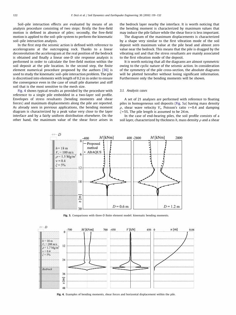
Envelopes of bending moments along the piles are presented inFig. 3. Results obtained with the proposed model are in very goodagreement with those of the refined finite element model. Thisdemonstrates the efficiency of the proposed model in predictingthe kinematic stress resultants in the piles. For this reason theproposed procedure is considered in the following applicationsinstead of the time-consuming refined finite element analysis.

3. Parametric investigation

A comprehensive parametric study is carried out to analyse theeffects of the kinematic interaction on the internal stress resultantsin floating and end-bearing single piles having the restrainedrotational degree of freedom at the head (fixed head). The mainparameters governing the dynamic response of piles such as thediameter, the properties of the soil (in terms of shear wave velocityand density) and the bedrock location are considered.

element model: application data.

ARTICLE IN PRESS

F. Dezi et al. / Soil Dynamics and Earthquake Engineering 30 (2010) 119–132122

Soil–pile interaction effects are evaluated by means of ananalysis procedure consisting of two steps: firstly the free-fieldmotion is defined in absence of piles; secondly, the free-fieldmotion is applied to the soil–pile system to perform the kinematicsoil–pile interaction analysis.

In the first step the seismic action is defined with reference toaccelerograms at the outcropping rock. Thanks to a lineardeconvolution the accelerogram at the real position of the bedrockis obtained and finally a linear one-D site response analysis isperformed in order to calculate the free-field motion within thesoil deposit at the pile location. In the second step, the finiteelement numerical procedure proposed by the authors [36] isused to study the kinematic soil–pile interaction problem. The pileis discretised into elements with length of 0.2 m in order to ensurethe convergence even in the case of small pile diameter and stiffsoil that is the most sensitive to the mesh size.

Fig. 4 shows typical results as provided by the procedure withreference to a single pile embedded in a two-layer soil profile.Envelopes of stress resultants (bending moments and shearforces) and maximum displacements along the pile are reported.As already seen in previous applications, the bending momentdiagram is characterized by a peak value very close to the layerinterface and by a fairly uniform distribution elsewhere. On theother hand, the maximum value of the shear force arises in

Fig. 3. Comparisons with three-D finite elem

Fig. 4. Examples of bending moments, shear force

the bedrock layer nearby the interface. It is worth noticing thatthe bending moment is characterized by maximum values thatmay induce the pile failure while the shear force is less important.

The diagram of the maximum displacements is characterizedby a shape very similar to the first vibration mode of the soildeposit with maximum value at the pile head and almost zerovalue near the bedrock. This means that the pile is dragged by thevibrating soil and that the stress resultants are mainly associatedto the first vibration mode of the deposit.

It is worth noticing that all the diagrams are almost symmetricowing to the cyclic nature of the seismic action. In considerationof the symmetry of the pile cross-section, the absolute diagramswill be plotted hereafter without losing significant information.Furthermore only the bending moments will be shown.

3.1. Analysis cases

A set of 21 analyses are performed with reference to floatingpiles in homogeneous soil deposits (Fig. 5a) having mass densityr, shear wave velocity Vs, Poisson’s ratio n=0.4 and dampingx=5%. The pile length is assumed to be 24 m.

In the case of end-bearing piles, the soil profile consists of asoil layer, characterized by thickness h, mass density r and a shear

ent model: kinematic bending moments.

s and horizontal displacement within the pile.

ARTICLE IN PRESS

Fig. 5. Analyses schemes: (a) homogeneous profile and (b) two-layered soil profile.

Table 1Parameters adopted in the analysis.

Vs (m/s) r (Mg/m3) D (m) h (m)

100, 200, 400 1.5, 1.7, 2.0 0.2, 0.4, 0.6, 0.8,

1.0, 1.5, 2.0

6, 12, 18, 30, 42

F. Dezi et al. / Soil Dynamics and Earthquake Engineering 30 (2010) 119–132 123

wave velocity Vs, overlying a rock stratum having mass densityrb=2.5 Mg/m3 and shear wave velocity Vsb=800 m/s (Fig. 5b).Both the layers are characterized by Poisson’s ratio n=nb=0.4. Thelow-strain shear modulus is considered in the analyses anddamping is assumed to be x=5%, for the deposit and xb=2% for thebedrock. The pile is assumed to be 48 m long and characterizedby Young’s modulus Ep=30000 N/mm2 and mass density rp=2.5Mg/m3.

Eight different pile diameters, five different bedrock locationsand three different shear wave velocities are considered for a totalof 120 cases (Table 1).

The analysis scenarios cover a wide range of possible two-layersoil profiles and make it possible to investigate the effects of thelayer interface on pile bending moments for highly contrastingsoil properties and various pile diameters.

3.2. Seismic motion

According to modern standards (e.g. Eurocode 8 [14]) sevenartificial or recorded accelerograms, characterized by a meanresponse spectrum matching the one suggested by the code, maybe used to represent the seismic action. Subsequently, the effectshave to be evaluated by averaging the results obtained from theseven analyses.

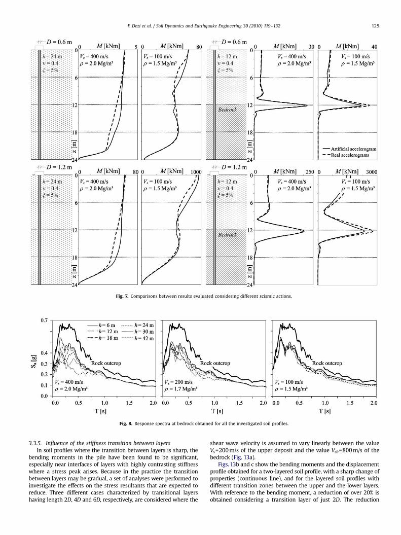
In this section the mean results obtained with the sevenaccelerograms shown by Fig. 6a–g are compared with thoseachieved by considering the artificial accelerogram given byFig. 6h matching the same spectrum. The graphs of Fig. 7 showthe envelopes of the bending moments arising along the pilesof diameters 0.6 and 1.2 m. Four soil stratigraphies, twohomogeneous (Vs=100 and 400 m/s) and two layered (h=12 m,Vs=100 and 400 m/s), are considered. Concerning thehomogeneous deposits the maximum bending moment recordedat the pile head is almost coincident even if some differences are

evident along the pile. In the layered profiles results revealed to bein very good agreement in the case of Vs=400 m/s whiledifferences up to 20%, concerning the maximum bendingmoment at the pile head and at the deposit-bedrock interface,are present in the case of Vs=100 m/s.

These comparisons reveal that in the case of linear kinematicinteraction analyses the set of seven accelerograms may besubstantially substituted by a single artificial accelerogram withsome differences in the case of soft soils.

In the sequel, the parametric investigation is performedassuming as input motion a single artificial accelerogram match-ing the EC8 Type 1 elastic response spectrum for ground type Aand PGA=0.25 g. Fig. 8 shows the response spectra obtained fromthe deconvolution analyses for all the soil profiles investigatedstarting from the selected artificial accelerogram; each graphrefers to a specific soil type and collects results obtained fordifferent thickness h of the deformable layer. In all the casesspectral de-amplifications are evident in correspondence of thefundamental periods of the soil deposits. It is worth noticing thatsoil profiles with Vs=400 m/s are particularly responsive to thedeconvolution process in the range 0.0–0.5 s where the periods ofthe soil deposits fall and where the spectrum of the seismic inputaction achieves the maximum values.

3.3. Main results

3.3.1. Embedment into the stiff layer

The effect of the pile embedment in the stiff layer isinvestigated with reference to a single pile of diameter 1.0 mand different soil profiles characterized by h=6, 12, 18 m andVs=100, 200 and 400 m/s. For each stratigraphy different pileembedments were assumed namely 1D, 3D and 5D. Attention isfocused on the pile behavior at the deposit–bedrock interface. It isimportant to point out that the same maximum bending momentis achieved for embedments greater that 3D (Fig. 9). In particular,the moment envelope along the pile for an embedment of 3D iscoincident with that of 5D except, quite obviously, for theexceeding pile length where negligible moments are attained.For the relative pile–bedrock stiffness considered, the previousresults suggest that the embedment of 3D is sufficient to providethe maximum degree of restraint at the pile base.

3.3.2. Influence of the pile diameter

The graphs in Fig. 10 show the distribution within the piledepth of the maximum absolute bending moments for the floatingpile and for end-bearing piles (h=6, 18, 42 m). Each graph collectsthe results obtained for different pile diameters and for a constantvalue of the shear wave velocity Vs.

In the case of floating piles the maximum bending moment isattained at the pile head. It is particularly significant for very softsoils (Vs=100 m/s) but reduces dramatically as the soil stiffnessincreases. Furthermore, the diagrams are characterised bydifferent shapes: in the case of soft soil, the bending momentincreases almost linearly from the end to the head of the pilewhile for rigid soils it increases only in the lower half pile andremains almost constant in the upper part.

In the case of end-bearing piles, bending moments assumemaximum values very close to the interface between the depositand the bedrock. In the case of the surface layer with small depth,a second peak arises at the pile head due to the restraint appliedin order to simulate the presence of the cap.

As expected, the pile diameter significantly affects theamplitude of the bending moments at the pile head and at theinterface between layers: for a given soil deposit, the bendingmoment increases as the pile diameter increases. Although the

ARTICLE IN PRESS

Fig. 6. (a–g) real accelerograms and (h) artificial accelerogram.

F. Dezi et al. / Soil Dynamics and Earthquake Engineering 30 (2010) 119–132124

distributions have very similar shapes it is worth noticing that thepeaks are characterised by different widths depending even onthe pile diameter.

3.3.3. Influence of the bedrock depth

With reference to end-bearing piles, the graphs in Fig. 11 showthe kinematic bending moments arising along the piles ofdifferent diameters for all the soil profiles considered. Eachgraph refers to a couple of shear wave velocity Vs and diameterD and groups results obtained for different values of h.

The bending moment at the deposit–bedrock interface in-creases with the depth whereas that at the pile head decreasesespecially in soft soil deposits (Vs=100 m/s).

It is worth noticing that the peak value of the bending momentincreases when the bedrock depth is less than 18 m whereas fordeeper bedrock the peak value remains nearly constant.

In many cases, the bending moment at the pile head iscomparable with that at the deposit–bedrock interface. It stronglydepends on all the parameters considered in the investigation. In

particular it is evident that for soft soils (Vs=100 and 200 m/s) thebending moment diagram is characterized by a double peak. Thehead peak reduces by increasing the bedrock depth as quickly asthe pile diameter reduces: for very large diameters (D=2.0 m) theeffect is still significant at bedrock depths of about 20 m.

3.3.4. Influence of the soil properties

To better understand the effect of the stiffness contrastbetween the two layers on the maximum bending moment, fiveshear wave velocities for the upper soil layer are considered(Vs=100, 150, 200, 300 and 400 m/s). The graphs of Fig. 12 showthe bending moment distributions obtained for three pilediameters and a constant value of the bedrock location h.As expected, the bending moments increase as the shear wavevelocity Vs decreases. Furthermore the phenomena previouslydescribed are evident: the width of the peak at deposit–bedrockinterface as well as the bending moment at the pile head increasesby increasing the pile diameter and reducing the soil stiffness.

ARTICLE IN PRESS

Fig. 7. Comparisons between results evaluated considering different scismic actions.

Fig. 8. Response spectra at bedrock obtained for all the investigated soil profiles.

F. Dezi et al. / Soil Dynamics and Earthquake Engineering 30 (2010) 119–132 125

3.3.5. Influence of the stiffness transition between layers

In soil profiles where the transition between layers is sharp, thebending moments in the pile have been found to be significant,especially near interfaces of layers with highly contrasting stiffnesswhere a stress peak arises. Because in the practice the transitionbetween layers may be gradual, a set of analyses were performed toinvestigate the effects on the stress resultants that are expected toreduce. Three different cases characterized by transitional layershaving length 2D, 4D and 6D, respectively, are considered where the

shear wave velocity is assumed to vary linearly between the valueVs=200 m/s of the upper deposit and the value Vsb=800 m/s of thebedrock (Fig. 13a).

Figs. 13b and c show the bending moments and the displacementprofile obtained for a two-layered soil profile, with a sharp change ofproperties (continuous line), and for the layered soil profiles withdifferent transition zones between the upper and the lower layers.With reference to the bending moment, a reduction of over 20% isobtained considering a transition layer of just 2D. The reduction

ARTICLE IN PRESS

Fig. 9. Effects of the pile embedment in the bedrock on the bending moment.

F. Dezi et al. / Soil Dynamics and Earthquake Engineering 30 (2010) 119–132126

reaches 50% when the transition layer is 6D thick. It is worth noti-cing that the peaks become considerably smoother and that themaximum values translate upwards. This may be understood byobserving the pile displacement profiles that are characterised bylower curvatures as the transition layer becomes thicker. Finally, thebending moments at the pile section far from the transition layer arenot affected by the thickness of the transition layer.

4. Empirical design formulas

With reference to kinematic pile bending moments at theinterface between soil layers, Nikolaou et al. [15] presented acritical review of the design methods proposed by Marganson [34]and Dobry and O’Rourke [4] pointing out some drawbacks. Thefirst considers the pile subjected to the soil curvatures encounter-

ing problems with the interface between different layers. Thesecond assumes harmonic excitations obtaining results thatoverestimate those of transient shakings. Nikolaou et al. [15]propose an expression for evaluating the maximum steady-statebending moment at the interface of the layers and introduce acoefficient to adjust the results in the case of real seismic motions,overcoming the limits of the previous formulations. However noformula is presented to calculate the bending moment at the pilehead.

In order to find empirical formulas to predict the kine-matic bending moments at the pile head and at the interfacebetween bedrock and deposit, the results are normalized withrespect to the values obtained for the stiffer soil (Vs=400 m/s).

Figs. 14 and 15 show the maximum normalised kinematicbending moments at the pile head and at the deposit–bedrockinterface, respectively, versus the shear wave velocity of the upper

ARTICLE IN PRESS

Fig. 10. Effects of pile diameter on bending moments: (a) floating piles and (b–d) end-bearing piles.

F. Dezi et al. / Soil Dynamics and Earthquake Engineering 30 (2010) 119–132 127

ARTICLE IN PRESS

Fig. 11. Effects of the bedrock depth on bending moments: (a) D=0.4 m, (b) D=0.8 m, (c) D=1.2 m and (d) D=2.0 m.

F. Dezi et al. / Soil Dynamics and Earthquake Engineering 30 (2010) 119–132128

ARTICLE IN PRESS

Fig. 12. Influence of the soil characteristics on bending moments.

Fig. 13. Effects of stiffness transition between layers: (a) cases analysed, (b) bending moment envelope and (c) profiles of displacements.

F. Dezi et al. / Soil Dynamics and Earthquake Engineering 30 (2010) 119–132 129

soil layer. Values M400 of absolute bending moments obtainedwith Vs=400 m/s are also reported.

With reference to the pile head (Fig. 14) three remarks may bemade: (i) the values of M400 are only slightly dependent on h

whereas they are very sensitive to the pile diameter; (ii) for eachdeposit depth h, diagrams of normalised bending moments versusVs are superimposed for the different pile diameters and arecharacterised by an exponential trend; (iii) only for soft soils(Vs=100–200 m/s) and low-depth deposits (h=6 m) a dependencyon the pile diameter is evident.

With reference to the bending moment at the deposit–bedrockinterface (Fig. 15), values of M400 are more sensitive to the depositthickness whereas the above considerations hold for the normalisedbending moments.

These remarks suggest that an empirical expression of thebending moments, both at the head and at deposit–bedrockinterface, may have the following form:

MðVs;D;h; PGAÞffiPGA

0:25 gM400ðD;hÞe

f ðD;hÞðVs�400Þ ð15Þ

where the ratio PGA/0.25 g accounts for different seismicintensities owing to the problem linearity. Formulas for evaluating

bending moments M400(D, h) and the function f(D, h), defining thedependency of the exponential regression on D and h, arecalibrated with a nonlinear least square procedure by fitting thedata obtained in the parametric analysis.

With reference to the maximum bending moment at theinterface between bedrock and deposit, the following polynomialapproximations hold:

M400ðD;hÞ ¼ ð77:7D3þ409D2 � 192Dþ24:5Þ

�ð�0:0009h2þ0:068h� 0:2Þ ð16Þ

f ðD;hÞ ¼ ð0:000124h� 0:01106Þð�0:05Dþ0:864Þ ð17Þ

On the other hand, with reference to the maximumbending moment at the pile head, the following expressions areobtained:

M400ðD;hÞ ¼ ð85D3 � 85:75D2þ30:93D� 3:37Þ

�ð0:000133h2 � 0:00042hþ1:091Þ ð18Þ

f ðD;hÞ ¼ ð0:000067h� 0:0113Þð�0:07Dþ1:002Þ ð19Þ

ARTICLE IN PRESS

Fig. 14. Normalized bending moments at the pile head.

Fig. 15. Normalized bending moments at the deposit–bedrock interface.

F. Dezi et al. / Soil Dynamics and Earthquake Engineering 30 (2010) 119–132130

Eq. (15) permits predicting straightforward the bending mo-ments at the critical sections of an end-bearing pile embeddedin a generic homogeneous soil by knowing the PGA asso-

ciated to the soil of class A as defined in EC8 [14], the velocityof the shear wave of the deposit, the pile diameter and thebedrock depth. It is worth noticing that formula (15) accounts

ARTICLE IN PRESS

Fig. 16. Comparisons between theoretical and design formula (26) results: (a) at pile head and (b) at deposit–bedrock interface.

F. Dezi et al. / Soil Dynamics and Earthquake Engineering 30 (2010) 119–132 131

both for the local site response and the soil–pile kinematicinteraction.

Fig. 16 gives a comparison of the results obtained by applyingthe formula (15) with those obtained with the analyticalprocedure proposed in the first section, validated in Ref. [36],and compared with three-D finite element models in this paper.The discrepancies are generally acceptable for design purposes.Less precision is obtained for bending moments at the head ofpiles with a very small diameter. Fig. 16b gives a comparison withthe results obtained by also applying the formula of Nikolaou et al.[15] (white dots) that is able to predict kinematic bendingmoments only at the deposit–bedrock interface. As may benoticed, the proposed formula (15) gives better results.

5. Conclusions

The effects of kinematic interaction on the bending moment insingle end-bearing and floating piles have been studied. Anumerical procedure proposed by the authors [36] has been usedin performing a comprehensive parametric analysis by consider-ing different pile diameters, bedrock depths and shear wavevelocity of the deposit. Furthermore, design empirical formulashave been proposed to evaluate the kinematic bending momentsat the pile head and at the deposit–bedrock interface.

The seismic action is defined with reference to outcroppingbedrock by considering artificial accelerograms matching theEurocode 8 Type 1 elastic response spectrum for ground type A[14]. Shaking at the actual bedrock depth is calculated by a lineardeconvolution and the ground motion within the soil deposit isobtained with a linear one-D site response analysis.

The following conclusions may be drawn from the parametricanalysis:

�

For the relative pile–bedrock stiffness considered in this paper,the embedment of 3D is sufficient to provide the maximumdegree of restraint at the pile base. � The peak values of the bending moment in the pile, at the

interface between the deposit and the bedrock, increase withthe pile diameter and the thickness of the surface soil layer aswell as with the stiffness contrast between layers.

� For small values of the surface soil layer thickness, the

maximum bending moment arises at the pile head instead ofat the layer interface.

�

The bending moments at pile head and at layer interfacesharply reduce as the shear wave velocity increases and � A reduction of the bending moment is obtained considering

soil profiles with transition layers instead of a sharp change ofproperties. Bending moment peaks become considerablysmoother and wider.

On the basis of the parametric analysis, new design formulas

for predicting the kinematic bending moment in end-bearing pileshave been proposed. They are valid both for the cross-sections atthe pile head and at the interface between the soil deposit and thebedrock. Their application is straightforward since few para-meters, namely the PGA, the bedrock depth, the shear wavevelocity of the soil deposit and the pile diameter, are necessary.Local site response effects are accounted for without having toperform specific analyses. The comparisons with the analyticalsolutions are very satisfactory.

References

[1] Ishihara K. Soil behavior in earthquake geotechnics. Oxford: Clarendon Press;1996.

[2] Kagawa T, Kraft LM. Lateral load-deflection relationships of piles subjected todynamic loads. Soils and Foundations 1980;20(4):19–36.

[3] Flores-Berrones R, Whitman RV. Seismic response of end-bearing piles.Journal of the Geotechnical Engineering Division—ASCE 1982;108(4):554–69.

[4] Dobry R, O’Rourke MJ. Discussion on ‘‘Seismic response of end-bearing piles’’by Flores Berrones R. and Whitman R.V. Journal of the GeotechnicalEngineering Division—ASCE 1983;109(5):778–81.

[5] Mineiro AJC. Simplified procedure for evaluating earthquake loading on piles.Lisbon: De Mello Volume; 1990.

[6] Novak M. Piles under dynamic loads: state of the art. In: Proceedings of the2nd international conference on recent advances in geotechnical earthquakeengineering and soil dynamics. USA: St. Louis; 1991. p. 2433–56.

[7] Kavvadas M, Gazetas G. Kinematic seismic response and bending of free-headpiles in layered soil. Geotechnique 1993;43(2):207–22.

[8] Pender M. Seismic pile foundation design analysis. Bulletin of the NewZealand National Society for Earthquake Engineering 1993;26(1):49–160.

[9] Kaynia AM, Mahzooni S. Forces in pile foundations under seismic loading.Journal of Engineering Mechanics ASCE 1996;122(1):46–53.

[10] Poulos HG, Tabesh A. Seismic response of pile foundations—some importantfactors. In: Proceedings of the 11th WCEE. Acapulco, Mexico; 1996. Paper no.2085.

[11] Gazetas G, Mylonakis G. Seismic soil–structure interaction: new evidence andemerging issues. Geotechnical earthquake engineering & soil dynamics. In:Proceedings of the third Geo-Institute ASCE conference, vol. II, Seattle, USA,1998. p. 1119–74.

[12] Milonakis G. Simplified model for seismic pile bending at soil layer interfaces.Soils and Foundations 2001;41(4):47–58.

ARTICLE IN PRESS

F. Dezi et al. / Soil Dynamics and Earthquake Engineering 30 (2010) 119–132132

[13] Banerjee PK, Davies TG. The behaviour of axially and laterally loadedsingle piles embedded in nonhomogeneous soils. Geotechnique 1978;28(3):309–26.

[14] En 1998-1. Eurocode 8 – design of structure for earthquake resistance – part1: general rules, seismic actions and rules for buildings. European Committeefor Standardization; 2004.

[15] Nikolaou AS, Mylonakis G, Gazetas G, Tazoh T. Kinematic pile bending duringearthquakes analysis and field measurements. Geotecnique 2001;51(5):425–40.

[16] Mylonakis G. Contributions to static and seismic analysis of piles and pile-supported bridge piers. Ph.D. Thesis, State University of New York, USA, 1995.

[17] Sica S, Mylonakis G, Simonelli AL. Kinematic bending moments of piles:analysis vs. code provisions. In: Proceedings of the 4th International Conferenceon Earthquake Geotechnical Engineering. Tessaloniki, Greece; 2007.

[18] Wolf JP. Dynamic soil–structure-interaction. Englewood Cliffs, New Jersey:Prentice-Hall Inc.; 1985.

[19] Maeso O, Aznarez JJ, Garcıa F. Dynamic impedances of piles and groups ofpiles in saturated soils. Computers and Structures 2005;83:769–82.

[20] Coda HB, Venturini WS. On the coupling of 2D BEM and FEM frame modelapplied to elastodynamic analysis. International Journal of Solids andStructures 1999;36:4789–804.

[21] Millan MA, Domınguez J. Simplified BEM/FEM model for dynamic analysis ofstructures on piles and pile groups in viscoelastic and poroelastic soils.Engineering Analysis with Boundary Elements 2009;33:25–34.

[22] Padron LA, Aznarez JJ, Maeso O. Dynamic analysis of piled foundations instratified soils by a BEM–FEM model. Soil Dynamics and EarthquakeEngineering 2008;28(5):333–46.

[23] Maheshwari BK, Truman KZ, El Naggar MH, Gould PL. Three-dimensionalnonlinear analysis for seismic soil–pile-structure interaction. Soil Dynamicsand Earthquake Engineering 2004;24(4):343–56.

[24] Sadek M, Isam S. Three-dimensional finite element analysis of the seismicbehavior of inclined micropiles. Soil Dynamics and Earthquake Engineering2004;24(6):473–85.

[25] Jeremic B, Jie G, Preisig M, Tafazzoli N. Time domain simulation of soil–foundation–structure interaction in non-uniform soils. Earthquake Engineer-ing and Structural Dynamics 2009;38:699–718.

[26] Kuc- ukarslan S, Banerjee PK. Behavior of axially loaded pile group underlateral cyclic loading. Engineering Structures 2003;25:303–11.

[27] Matlock H, Foo SH, Bryant LL. Simulation of lateral pile behaviour. In:Proceedings of earthquake engineering and soil dynamics, ASCE. Pasadena,California; 1978. p. 600–19.

[28] Nogami T, Chen HL. Prediction of dynamic lateral response of non linearsingle pile by using Winkler soil model. In: Proceedings of the session ondynamic response of pile foundations-experiment, analysis, and observation;Geotechnical special publication no. 11, ASCE. Atlantic City, New Jersey; 1987.p. 39–52.

[29] Novak M. Dynamic stiffness and damping of piles. Canadian GeotechnicalJournal 1974;11:574–97.

[30] Makris N, Gazetas G. Dynamic pile–soil–pile interaction-part II: lateral andseismic response. Earthquake Engineering and Structural Dynamics1992;21(2):145–62.

[31] Romo MP, Ovando-Shelley E. P–Y curves for piles under seismic lateral loads.Geotechnical and Geological Engineering 1999;16(4):251–72.

[32] Rovithis E, Kirtas E, Pitilakis K. Experimental p–y loops for estimating seismicsoil–pile interaction. Bulletin of Earthquake Engineering 2009;7(3):719–36.

[33] Catal HH. Free vibration of semi-rigid connected and partially embedded pileswith the effects of the bending moment, axial and shear force. EngineeringStructures 2006;28(14):1911–8.

[34] Margason E. Pile bending during earthquakes. Lecture, 6 March 1975, ASCE-UC/Berkeley Seminar on Design Construction and Performance of DeepFoundations (unpublished).

[35] Dente G. Pile foundations; guidelines on geotechnical aspects for designing inseismic areas. Bologna, Italy: Patron Editore; 2005 (in Italian).

[36] Dezi F, Carbonari S, Leoni G. A model for the 3D kinematic interaction analysisof pile groups in layered soils. Earthquake Engineering and StructuralDynamics 2009;38(11):1281–305.

[37] Gazetas G, Dobry R. Horizontal response of piles in layered soils. Journal ofGeotechnical Engineering ASCE 1984;110:20–40.

[38] Roesset JM, Angelides D. Dynamic stiffness of piles. In: Numerical methods inoffshore piling. CE, London; 1989. p. 75–81.

[39] Krishnan R, Gazetas G, Velez A. Static and dynamic lateral deflections of pilesin non-homogeneous stratum. Geotechnique 1983;23(3):307–25.

[40] Gazetas G, Dobry R. Single radiation damping model for piles and footings.Journal of Engineering Mechanics ASCE 1984;110:937–56.

[41] Kramer SL. Geotechnical earthquake engineering. Englewood Cliffs, NJ:Prentice-Hall; 1996.