Kinematics of star formation in evolving galaxies · turbulent, in marked contrast to modern...

Kinematics of Star Formation inEvolving Galaxies

Andrew Green

Presented in fulfillment of the requirementsof the degree of Doctor of Philosophy

Original submission: 2 September 2011Revised version: 15 February 2012

Accepted: 5 March 2012

Faculty of Information and Communication TechnologySwinburne University of Techonology

for my father and mother

Abstract

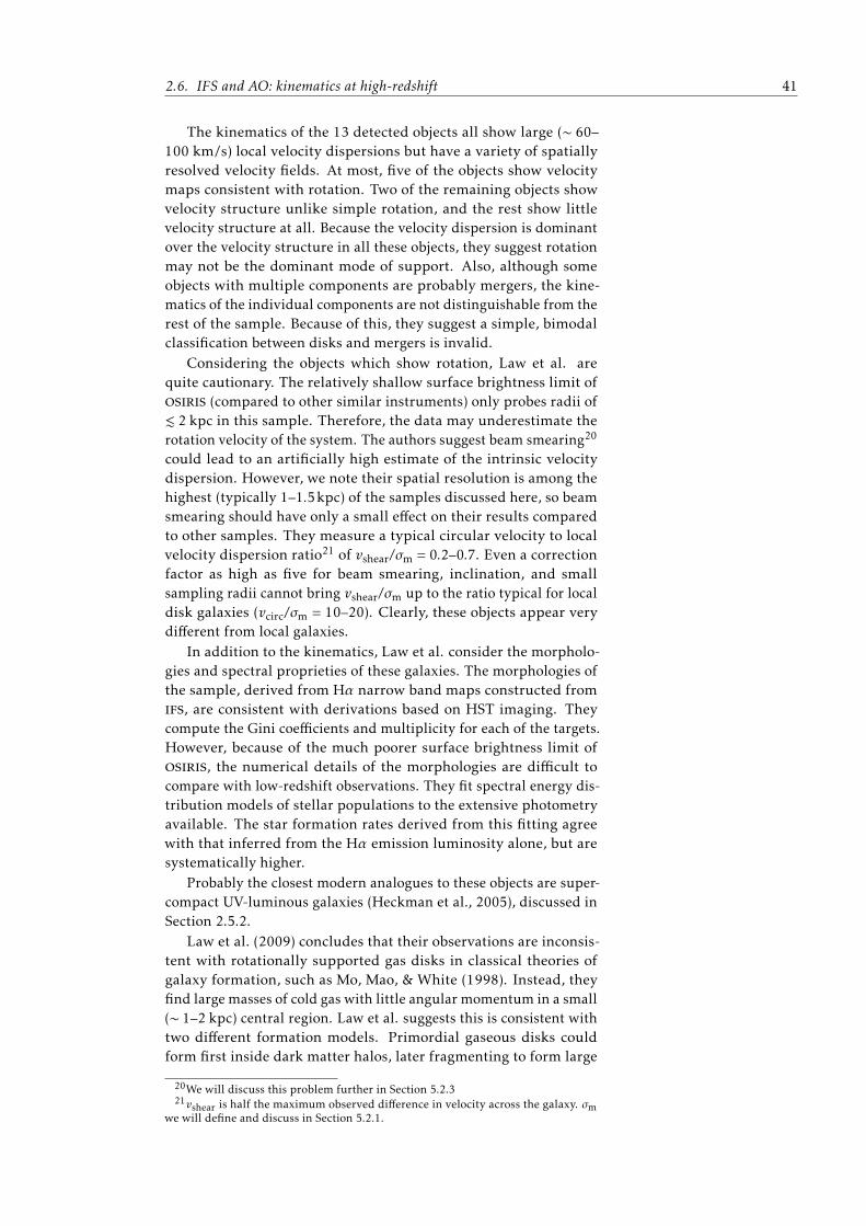
This work explores how the kinematics of star forming galaxies in the modern epochcompare with earlier galaxies. It focuses on what physical processes are responsible for thedifferences in galaxies between epochs. It also validates new observational techniques acrossa large range in kinematic properties. Previous works have found early galaxies to be highlyturbulent, in marked contrast to modern galaxies. Those works argue the accumulation ofstellar mass and the changing gas accretion rates drive the evolution of galaxies between earlyand modern states. Theoreticians have postulated several mechanisms of galaxy assembly,which can explain the observed evolution. Debate centres around exactly which physicalprocesses give rise to the kinematic states of observed galaxies, whether the processes differwith epoch, and how observations bias the observations. This thesis explores a broaderrange in kinematic states in modern galaxies than previously considered in a single sample.A simple selection from a large sample of galaxies makes this range possible. Integralfield spectroscopy provides observations commensurate with previous work. A handful ofgalaxies in this sample show kinematics very similar to galaxies observed at early epochs,while the remainder are more representative of modern galaxies. This work also finds starformation rate and gas turbulence are closely linked in galaxies at all epochs, but thesetwo phenomenon are not always spatially coincident within galaxies. It identifies highlyturbulent, clumpy star forming disk galaxies in the modern Universe—objects previouslythought non-existent. This work also validates, in a controlled environment, the newobservational techniques commonly used on early galaxies. The continued presence of highlyturbulent disk galaxies in the modern epoch provides new constraints on galaxy evolutionmodels. The previously unknown correlation between star formation and turbulence ingalaxies indicates the important physical link between these two processes. These resultsprovide new constraints for future models of galaxy evolution.

iii

Acknowledgements

I would like to acknowledge the extensive ideas, advice, criticism and support provided byKarl Glazebrook. Without his guidance, this work would not be what it is.

I also acknowledge a special scholarship from the Chancellery of the Swinburne Universityof Technology for making it possible to start this project early.

Alison Thomson, Lincoln Smith, Emily Willocks, and Avan Barker also helped edit andimprove this text, help which I greatly appreciated. I also thank my friends for their kindunderstanding as I prepared this thesis.

Most importantly, I appreciate all the care and support of my parents, Ron and Nancy Green,who always encourage me to follow my dreams.

Some of the data presented herein were obtained at the W.M. Keck Observatory, whichis operated as a scientific partnership among the California Institute of Technology, theUniversity of California and the NASA. The Observatory was made possible by the generousfinancial support of the W.M. Keck Foundation.

v

Declaration

I declare that this examinable outcome

• contains no material which has been accepted for the award to myself of any otherdegree or diploma;

• to the best of my knowledge contains no material previously published or written byanother person except where due reference is made in the this text; and

• where sections of this document are based on joint research or publications, the relativecontributions of the respective workers or authors is as set out in Section 1.2.

Andrew Wesley Green

vii

Contents

Abstract iii

Contents ixList of Figures . . . . . . . . . . . . . . . . . . . . . . . . . . . . . . . . . . . . . . . xiiiList of Tables . . . . . . . . . . . . . . . . . . . . . . . . . . . . . . . . . . . . . . . . xvii

1 Introduction 11.1 Goals of this thesis . . . . . . . . . . . . . . . . . . . . . . . . . . . . . . . . . . 11.2 Contributions from others . . . . . . . . . . . . . . . . . . . . . . . . . . . . . 21.3 Previously published work . . . . . . . . . . . . . . . . . . . . . . . . . . . . . 31.4 Brief plan of this thesis . . . . . . . . . . . . . . . . . . . . . . . . . . . . . . . 3

2 Background 52.1 Star forming galaxies and their evolution . . . . . . . . . . . . . . . . . . . . . 6

2.1.1 What is a star forming galaxy? . . . . . . . . . . . . . . . . . . . . . . . 62.1.2 Characterising the makeup of a galaxy spectroscopically . . . . . . . 82.1.3 Morphologies . . . . . . . . . . . . . . . . . . . . . . . . . . . . . . . . 82.1.4 Where star formation occurs . . . . . . . . . . . . . . . . . . . . . . . . 102.1.5 What we know about star formation in galaxies . . . . . . . . . . . . . 112.1.6 Star formation in the context of galaxy evolution . . . . . . . . . . . . 14

2.2 Galaxy kinematics and the Tully Fisher Relation . . . . . . . . . . . . . . . . . 152.2.1 Kinematic morphologies . . . . . . . . . . . . . . . . . . . . . . . . . . 182.2.2 Kinematics of star formation . . . . . . . . . . . . . . . . . . . . . . . . 192.2.3 The Tully Fisher Relation . . . . . . . . . . . . . . . . . . . . . . . . . . 212.2.4 DEEP2 and S0.5 . . . . . . . . . . . . . . . . . . . . . . . . . . . . . . . 22

2.3 Integral field spectroscopy . . . . . . . . . . . . . . . . . . . . . . . . . . . . . 232.3.1 Types of integral field spectroscopy . . . . . . . . . . . . . . . . . . . . 242.3.2 Early IFS work . . . . . . . . . . . . . . . . . . . . . . . . . . . . . . . . 29

2.4 Adaptive optics . . . . . . . . . . . . . . . . . . . . . . . . . . . . . . . . . . . 312.5 Contemporary IFS work in the nearby Universe . . . . . . . . . . . . . . . . . 33

2.5.1 GHASP: The local Universe in Hα . . . . . . . . . . . . . . . . . . . . . 332.5.2 Lyman Break Analogues at z = 0.2 . . . . . . . . . . . . . . . . . . . . . 352.5.3 SAURON: The 2D kinematics of elliptical galaxies . . . . . . . . . . . 36

2.6 IFS and AO: kinematics at high-redshift . . . . . . . . . . . . . . . . . . . . . 372.6.1 SINS Survey . . . . . . . . . . . . . . . . . . . . . . . . . . . . . . . . . 382.6.2 Dispersion dominated BX galaxies . . . . . . . . . . . . . . . . . . . . 402.6.3 IMAGES . . . . . . . . . . . . . . . . . . . . . . . . . . . . . . . . . . . 422.6.4 MASSIV: The VVDS at z ∼ 1.5 . . . . . . . . . . . . . . . . . . . . . . . 432.6.5 VVDS at z > 3 . . . . . . . . . . . . . . . . . . . . . . . . . . . . . . . . 442.6.6 Gravitationally lensed objects . . . . . . . . . . . . . . . . . . . . . . . 46

ix

x Contents

2.6.7 WiggleZ super starbursts . . . . . . . . . . . . . . . . . . . . . . . . . . 472.6.8 Common themes in high-redshift IFS observations . . . . . . . . . . . 47

2.7 Need for more work in the local Universe . . . . . . . . . . . . . . . . . . . . 48

3 Observations and data analysis techniques 513.1 Sample selection motivation . . . . . . . . . . . . . . . . . . . . . . . . . . . . 51

3.1.1 Bias in high-redshift galaxy samples . . . . . . . . . . . . . . . . . . . 523.1.2 Restrictions imposed by IFS . . . . . . . . . . . . . . . . . . . . . . . . 533.1.3 Impact on results . . . . . . . . . . . . . . . . . . . . . . . . . . . . . . 55

3.2 Target selection at low redshift . . . . . . . . . . . . . . . . . . . . . . . . . . . 563.2.1 Parent sample: The Sloan Digital Sky Survey . . . . . . . . . . . . . . 563.2.2 Criteria and selected galaxies . . . . . . . . . . . . . . . . . . . . . . . 583.2.3 Properties of selected galaxies . . . . . . . . . . . . . . . . . . . . . . . 62

3.3 Target selection at high redshift . . . . . . . . . . . . . . . . . . . . . . . . . . 643.3.1 Parent sample: The Gemini Deep Deep Survey . . . . . . . . . . . . . 653.3.2 Criteria and selected galaxies . . . . . . . . . . . . . . . . . . . . . . . 663.3.3 Properties of selected galaxies . . . . . . . . . . . . . . . . . . . . . . . 68

3.4 Observations . . . . . . . . . . . . . . . . . . . . . . . . . . . . . . . . . . . . . 703.4.1 SPIRAL . . . . . . . . . . . . . . . . . . . . . . . . . . . . . . . . . . . . 713.4.2 WiFeS . . . . . . . . . . . . . . . . . . . . . . . . . . . . . . . . . . . . . 723.4.3 OSIRIS . . . . . . . . . . . . . . . . . . . . . . . . . . . . . . . . . . . . 743.4.4 NIFS . . . . . . . . . . . . . . . . . . . . . . . . . . . . . . . . . . . . . 79

3.5 Basic data reduction . . . . . . . . . . . . . . . . . . . . . . . . . . . . . . . . . 833.5.1 SPIRAL . . . . . . . . . . . . . . . . . . . . . . . . . . . . . . . . . . . . 833.5.2 WiFeS . . . . . . . . . . . . . . . . . . . . . . . . . . . . . . . . . . . . . 873.5.3 OSIRIS . . . . . . . . . . . . . . . . . . . . . . . . . . . . . . . . . . . . 893.5.4 NIFS . . . . . . . . . . . . . . . . . . . . . . . . . . . . . . . . . . . . . 91

3.6 Advanced data analysis . . . . . . . . . . . . . . . . . . . . . . . . . . . . . . . 943.6.1 Emission line fitting . . . . . . . . . . . . . . . . . . . . . . . . . . . . 943.6.2 Apertures and masks . . . . . . . . . . . . . . . . . . . . . . . . . . . . 953.6.3 Fit maps . . . . . . . . . . . . . . . . . . . . . . . . . . . . . . . . . . . 963.6.4 Line maps . . . . . . . . . . . . . . . . . . . . . . . . . . . . . . . . . . 983.6.5 Disk fitting . . . . . . . . . . . . . . . . . . . . . . . . . . . . . . . . . . 98

4 Integrated properties of star forming galaxies 1014.1 Star formation rates . . . . . . . . . . . . . . . . . . . . . . . . . . . . . . . . . 102

4.1.1 Hα luminosities . . . . . . . . . . . . . . . . . . . . . . . . . . . . . . . 1024.1.2 Dust extinction correction . . . . . . . . . . . . . . . . . . . . . . . . . 1024.1.3 Star formation rate estimation . . . . . . . . . . . . . . . . . . . . . . . 104

4.2 Gas masses . . . . . . . . . . . . . . . . . . . . . . . . . . . . . . . . . . . . . . 1054.2.1 Gas fractions . . . . . . . . . . . . . . . . . . . . . . . . . . . . . . . . . 106

4.3 Aperture effects . . . . . . . . . . . . . . . . . . . . . . . . . . . . . . . . . . . 1074.3.1 Hα and our selection method . . . . . . . . . . . . . . . . . . . . . . . 1074.3.2 Star formation rates . . . . . . . . . . . . . . . . . . . . . . . . . . . . . 110

4.4 Detecting clumps in the ISM spatially . . . . . . . . . . . . . . . . . . . . . . . 111

Contents xi

5 Kinematics 1175.1 Kinematic classifications . . . . . . . . . . . . . . . . . . . . . . . . . . . . . . 117

5.1.1 Visual classification using kinematic maps . . . . . . . . . . . . . . . . 1185.1.2 Disk model residuals . . . . . . . . . . . . . . . . . . . . . . . . . . . . 1215.1.3 Effect of resolution on classification . . . . . . . . . . . . . . . . . . . . 122

5.2 Velocity dispersion . . . . . . . . . . . . . . . . . . . . . . . . . . . . . . . . . 1255.2.1 The flux weighted mean local velocity dispersion (σm) . . . . . . . . . 1265.2.2 Statistical error in σm . . . . . . . . . . . . . . . . . . . . . . . . . . . . 1285.2.3 The effect of unresolved velocity gradients on σm . . . . . . . . . . . . 1285.2.4 A correction for σm . . . . . . . . . . . . . . . . . . . . . . . . . . . . . 1315.2.5 Other measures of velocity dispersion . . . . . . . . . . . . . . . . . . 133

5.3 The Tully Fisher Relation . . . . . . . . . . . . . . . . . . . . . . . . . . . . . . 1365.3.1 r-band Tully Fisher Relation . . . . . . . . . . . . . . . . . . . . . . . . 1375.3.2 Stellar mass Tully Fisher Relation . . . . . . . . . . . . . . . . . . . . . 1395.3.3 The S0.5 correction . . . . . . . . . . . . . . . . . . . . . . . . . . . . . 1395.3.4 Offsets and agreement . . . . . . . . . . . . . . . . . . . . . . . . . . . 1405.3.5 Interplay of the TFR, star formation, and turbulence . . . . . . . . . . 141

5.4 Disk stability criteria . . . . . . . . . . . . . . . . . . . . . . . . . . . . . . . . 1435.4.1 Toomre Q . . . . . . . . . . . . . . . . . . . . . . . . . . . . . . . . . . 143

5.5 Detecting clumps in the ISM spectroscopically . . . . . . . . . . . . . . . . . 1465.5.1 Dispersion among many distinct, quiescent clumps . . . . . . . . . . . 1465.5.2 Velocity shear broadening . . . . . . . . . . . . . . . . . . . . . . . . . 1485.5.3 Detecting clumps in real galaxies . . . . . . . . . . . . . . . . . . . . . 148

6 Star formation and turbulence 1516.1 Relationship between star formation rate and velocity dispersion . . . . . . . 151

6.1.1 A dichotomy . . . . . . . . . . . . . . . . . . . . . . . . . . . . . . . . . 1526.1.2 Initial discovery . . . . . . . . . . . . . . . . . . . . . . . . . . . . . . . 1546.1.3 The available data . . . . . . . . . . . . . . . . . . . . . . . . . . . . . . 1566.1.4 Resiliency of correlation . . . . . . . . . . . . . . . . . . . . . . . . . . 1586.1.5 Alternate measures of velocity dispersion . . . . . . . . . . . . . . . . 1626.1.6 Individual star forming regions . . . . . . . . . . . . . . . . . . . . . . 163

6.2 The link between star formation and turbulence . . . . . . . . . . . . . . . . . 1646.2.1 Mass and velocity dispersion . . . . . . . . . . . . . . . . . . . . . . . . 1646.2.2 Disk stability and σm . . . . . . . . . . . . . . . . . . . . . . . . . . . . 1656.2.3 Kinematic class and L(Hα) vs σm . . . . . . . . . . . . . . . . . . . . . 166

6.3 The spatial coincidence of star formation and turbulence . . . . . . . . . . . 1666.3.1 The pixel-to-pixel L–σ relation . . . . . . . . . . . . . . . . . . . . . . 1676.3.2 Maps of the coincidence of star formation and velocity dispersion . . 168

6.4 Physical explanations . . . . . . . . . . . . . . . . . . . . . . . . . . . . . . . . 1726.4.1 Fueling star formation . . . . . . . . . . . . . . . . . . . . . . . . . . . 1726.4.2 Driving turbulence . . . . . . . . . . . . . . . . . . . . . . . . . . . . . 1746.4.3 The dominant process . . . . . . . . . . . . . . . . . . . . . . . . . . . 176

7 Summary and future prospects 1797.1 Summary of major conclusions . . . . . . . . . . . . . . . . . . . . . . . . . . 1797.2 Impact of observational effects on recent IFS results . . . . . . . . . . . . . . 180

7.2.1 Results based on IFS vs long-slit spectroscopy . . . . . . . . . . . . . . 1807.2.2 Impact of AO on results . . . . . . . . . . . . . . . . . . . . . . . . . . 182

xii Contents

7.2.3 High-dispersion disk galaxies are not an observational artefact . . . . 1827.3 Are these galaxies “living dinosaurs”? . . . . . . . . . . . . . . . . . . . . . . 182

7.3.1 Implications for cold accretion . . . . . . . . . . . . . . . . . . . . . . 1837.4 Future directions . . . . . . . . . . . . . . . . . . . . . . . . . . . . . . . . . . 1847.5 Creating a complete picture . . . . . . . . . . . . . . . . . . . . . . . . . . . . 185

Bibliography 187

Notation 195

A Cosmology 197A.1 Co-moving distance . . . . . . . . . . . . . . . . . . . . . . . . . . . . . . . . . 197A.2 Luminosity distance . . . . . . . . . . . . . . . . . . . . . . . . . . . . . . . . . 198A.3 Angular diameter distance . . . . . . . . . . . . . . . . . . . . . . . . . . . . . 198A.4 Lookback time . . . . . . . . . . . . . . . . . . . . . . . . . . . . . . . . . . . . 198

B Maps of galaxies 199

C Tables 215

Publications derived from this work 225

Figure Credits 227

List of Figures

1.1 DYNAMO Nature cover . . . . . . . . . . . . . . . . . . . . . . . . . . . . . . . 3

2.1 Bimodality of star formation . . . . . . . . . . . . . . . . . . . . . . . . . . . . 72.2 Hubble’s Tuning Fork . . . . . . . . . . . . . . . . . . . . . . . . . . . . . . . . 82.3 Morphologies of early galaxies . . . . . . . . . . . . . . . . . . . . . . . . . . . 92.4 The Kennicutt-Schmidt Law . . . . . . . . . . . . . . . . . . . . . . . . . . . . 122.5 Star formation history of the Universe . . . . . . . . . . . . . . . . . . . . . . 142.6 30 Doradus . . . . . . . . . . . . . . . . . . . . . . . . . . . . . . . . . . . . . . 152.7 The first spectral map of Andromeda . . . . . . . . . . . . . . . . . . . . . . . 162.8 A spiral and an elliptical . . . . . . . . . . . . . . . . . . . . . . . . . . . . . . 182.9 Hβ and velocity dispersion in Hii regions . . . . . . . . . . . . . . . . . . . . 202.10 Cartoon of an IFS observation . . . . . . . . . . . . . . . . . . . . . . . . . . . 232.11 Fourier transform imaging spectrograph diagram . . . . . . . . . . . . . . . . 252.12 Schematic of a lenslet pupil array spectrograph . . . . . . . . . . . . . . . . . 272.13 Diagram of an image slicer . . . . . . . . . . . . . . . . . . . . . . . . . . . . . 282.14 SparsePak IFU . . . . . . . . . . . . . . . . . . . . . . . . . . . . . . . . . . . . 292.15 Velocity map of m51 . . . . . . . . . . . . . . . . . . . . . . . . . . . . . . . . . 302.16 The adaptive optics point spread function . . . . . . . . . . . . . . . . . . . . 322.17 Keck laser on fog . . . . . . . . . . . . . . . . . . . . . . . . . . . . . . . . . . . 322.18 Velocity map from GHASP . . . . . . . . . . . . . . . . . . . . . . . . . . . . . 332.19 Angular size with redshift . . . . . . . . . . . . . . . . . . . . . . . . . . . . . 372.20 SINS Survey overview . . . . . . . . . . . . . . . . . . . . . . . . . . . . . . . . 392.21 Galaxy from the IMAGES Sample . . . . . . . . . . . . . . . . . . . . . . . . . 422.22 Flat disk model . . . . . . . . . . . . . . . . . . . . . . . . . . . . . . . . . . . 442.23 Gravitationally lensed galaxy . . . . . . . . . . . . . . . . . . . . . . . . . . . 46

3.1 High-redshift selection effects . . . . . . . . . . . . . . . . . . . . . . . . . . . 543.2 Target selection windows at low-redshift . . . . . . . . . . . . . . . . . . . . . 583.3 Hα flux distribution of star forming galaxies in SDSS . . . . . . . . . . . . . . 593.4 Distribution of low-redshift targets in BPT . . . . . . . . . . . . . . . . . . . . 613.5 Telluric absorption and OH emission in the optical . . . . . . . . . . . . . . . 613.6 Selected SDSS galaxies . . . . . . . . . . . . . . . . . . . . . . . . . . . . . . . 633.7 Distribution of low-redshift targets in mass and star formation rate . . . . . 653.8 Keck adaptive optics field of view . . . . . . . . . . . . . . . . . . . . . . . . . 673.9 GDDS target selection . . . . . . . . . . . . . . . . . . . . . . . . . . . . . . . . 693.10 Images of selected GDDS galaxies . . . . . . . . . . . . . . . . . . . . . . . . . 703.11 The Anglo-Australian Telescope . . . . . . . . . . . . . . . . . . . . . . . . . . 713.12 The AAOmega Spectrograph . . . . . . . . . . . . . . . . . . . . . . . . . . . . 713.13 WiFeS Spectrograph . . . . . . . . . . . . . . . . . . . . . . . . . . . . . . . . . 72

xiii

xiv List of Figures

3.14 W.M. Keck Telescopes . . . . . . . . . . . . . . . . . . . . . . . . . . . . . . . . 753.15 OSIRIS observing sequence . . . . . . . . . . . . . . . . . . . . . . . . . . . . . 783.16 NIFS on Gemini North . . . . . . . . . . . . . . . . . . . . . . . . . . . . . . . 793.17 Closeup of the NIFS instrument . . . . . . . . . . . . . . . . . . . . . . . . . . 793.18 NIFS offset errors . . . . . . . . . . . . . . . . . . . . . . . . . . . . . . . . . . 813.19 Raw SPIRAL data . . . . . . . . . . . . . . . . . . . . . . . . . . . . . . . . . . 833.20 Observed Hα fluxes and SDSS . . . . . . . . . . . . . . . . . . . . . . . . . . . 863.21 Raw WiFeS data . . . . . . . . . . . . . . . . . . . . . . . . . . . . . . . . . . . 873.22 Data format on the OSIRIS detector . . . . . . . . . . . . . . . . . . . . . . . . 893.23 NIFS sky subtraction and bad pixel masking . . . . . . . . . . . . . . . . . . . 913.24 Cosmic ray on NIFS detector . . . . . . . . . . . . . . . . . . . . . . . . . . . . 923.25 Detector normal cosmic ray rejection . . . . . . . . . . . . . . . . . . . . . . . 933.26 Examples of fit spectra . . . . . . . . . . . . . . . . . . . . . . . . . . . . . . . 963.27 Spectra map of an SDSS galaxy . . . . . . . . . . . . . . . . . . . . . . . . . . 97

4.1 Dust corrections . . . . . . . . . . . . . . . . . . . . . . . . . . . . . . . . . . . 1044.2 Total star formation rate and mass . . . . . . . . . . . . . . . . . . . . . . . . . 1054.3 Galaxy gas fractions . . . . . . . . . . . . . . . . . . . . . . . . . . . . . . . . . 1064.4 Fibre field of view on an SDSS galaxy . . . . . . . . . . . . . . . . . . . . . . . 1074.5 Hα total and fibre aperture fluxes . . . . . . . . . . . . . . . . . . . . . . . . . 1094.6 Aperture corrections for SFR . . . . . . . . . . . . . . . . . . . . . . . . . . . . 1104.7 Pachen-α maps of HlumAz 10-2 . . . . . . . . . . . . . . . . . . . . . . . . . . 1124.8 Clump cluster galaxy at low-redshift . . . . . . . . . . . . . . . . . . . . . . . 1124.9 Example of clump fit in HlumAz 10–2 . . . . . . . . . . . . . . . . . . . . . . 114

5.1 Diagnostic diagrams for kinematic classification . . . . . . . . . . . . . . . . 1205.2 Disk fit χ2 values . . . . . . . . . . . . . . . . . . . . . . . . . . . . . . . . . . 1225.3 Velocity maps of high-χ2 objects classified as RD . . . . . . . . . . . . . . . . 1235.4 Effect of spatial resolution on kinematic results . . . . . . . . . . . . . . . . . 1245.5 A double-horned Hi emission line . . . . . . . . . . . . . . . . . . . . . . . . . 1255.6 Contribution of annuli around galaxies to flux weighted quantities . . . . . . 1305.7 Velocity dispersion and spatial resolution . . . . . . . . . . . . . . . . . . . . 1305.8 Effect of beam smearing on σm . . . . . . . . . . . . . . . . . . . . . . . . . . . 1325.9 Simulation of σint in widely seperated spectra . . . . . . . . . . . . . . . . . . 1345.10 Comparison of σsm and σm . . . . . . . . . . . . . . . . . . . . . . . . . . . . . 1355.11 The Tully Fisher Relation in a variety of observables . . . . . . . . . . . . . . 1385.12 Tully Fisher, star formation rate, and turbulence . . . . . . . . . . . . . . . . 1425.13 Toomre Q stability criterion . . . . . . . . . . . . . . . . . . . . . . . . . . . . 1445.14 Toomre Q and Tully Fisher Relation residuals . . . . . . . . . . . . . . . . . . 1455.15 Spectra from multiple simulated clumps . . . . . . . . . . . . . . . . . . . . . 1475.16 Simulated spectra map . . . . . . . . . . . . . . . . . . . . . . . . . . . . . . . 149

6.1 The dicotomy in velocity disperions . . . . . . . . . . . . . . . . . . . . . . . . 1526.2 Velocity dispersions and SFR of previous samples . . . . . . . . . . . . . . . . 1536.3 Initial Hα luminosity–velocity dispersion relation . . . . . . . . . . . . . . . . 1556.4 Compilation of σm and SFR data . . . . . . . . . . . . . . . . . . . . . . . . . . 1596.5 Hα luminosity as a function of different measures of velocity dispersion . . . 1616.6 Model velocity dispersion and star formation rates . . . . . . . . . . . . . . . 1636.7 Mass vs. local velocity dispersion . . . . . . . . . . . . . . . . . . . . . . . . . 165

List of Figures xv

6.8 Comparison of σm with Toomre Q andMbary . . . . . . . . . . . . . . . . . . 1666.9 Kinematic classifications and the SFR—σm relation . . . . . . . . . . . . . . . 1676.10 Local star formation rate compared with local turbulence . . . . . . . . . . . 1686.11 Spatial coincidence of star formation and turbulence . . . . . . . . . . . . . . 1706.12 Model of cold accretion . . . . . . . . . . . . . . . . . . . . . . . . . . . . . . . 1736.13 Stellar wind blowing a bubble in a gas cloud . . . . . . . . . . . . . . . . . . . 1746.14 The M81–M82 group . . . . . . . . . . . . . . . . . . . . . . . . . . . . . . . . 177

A.1 Co-moving distance approximation . . . . . . . . . . . . . . . . . . . . . . . . 198

B.1 Maps of galaxies . . . . . . . . . . . . . . . . . . . . . . . . . . . . . . . . . . . 200

List of Tables

3.1 Low Redshift selection categories. . . . . . . . . . . . . . . . . . . . . . . . . . 623.2 High redshift galaxy targets. . . . . . . . . . . . . . . . . . . . . . . . . . . . . 703.3 Observers for this program . . . . . . . . . . . . . . . . . . . . . . . . . . . . . 713.4 WiFeS Observations . . . . . . . . . . . . . . . . . . . . . . . . . . . . . . . . . 733.5 OSIRIS Observations . . . . . . . . . . . . . . . . . . . . . . . . . . . . . . . . 773.6 NIFS Observations . . . . . . . . . . . . . . . . . . . . . . . . . . . . . . . . . . 823.7 Summary of Disk Fitting Parameters . . . . . . . . . . . . . . . . . . . . . . . 99

4.1 Star Formation Properties . . . . . . . . . . . . . . . . . . . . . . . . . . . . . 1084.2 Clump sizes in HlumAz 10-2 . . . . . . . . . . . . . . . . . . . . . . . . . . . . 113

5.1 Kinematic Classifications . . . . . . . . . . . . . . . . . . . . . . . . . . . . . . 1215.2 Velocity dispersion properties of z ∼ 0.1 sample. . . . . . . . . . . . . . . . . . 127

A.1 Adopted cosmological parameters . . . . . . . . . . . . . . . . . . . . . . . . . 197

C.1 Summary of Low Redshift Targets. . . . . . . . . . . . . . . . . . . . . . . . . 216C.2 Previously known properties of Low Redshift Targets. . . . . . . . . . . . . . 218C.3 Disk parameters. . . . . . . . . . . . . . . . . . . . . . . . . . . . . . . . . . . . 220C.4 SPIRAL Observations . . . . . . . . . . . . . . . . . . . . . . . . . . . . . . . . 222

xvii

1Introduction

The nature of the evolution of galaxies remains a major unsolvedproblem in astronomy. Although there are many descriptions ofhow galaxies might evolve, none are universally accepted by theastronomy community. This thesis provides several significant newresults on the evolution of star forming galaxies.

Perhaps the greatest hindrance to progress in galaxy evolution isthe great timescales and physical scales involved. As with geology,most of the timescales greatly exceed the human lifetime, or evenhuman history. Like the ‘fossil record’ of geology, astronomers cansee most of the history of the Universe in the objects visible in thesky. Light takes time to travel from distant objects, so we can lookback in time by observing more distant objects. The expansion of theUniverse encodes in that light the time when it was emitted. Thus,astronomers can piece together the puzzle of galaxy evolution byobserving statistical samples of galaxies at different epochs.

The assembly of galaxies from the primordial gas present justafter the Big Bang is fundamentally a question of star formation.Galaxies are composed of stars, and those stars form in clouds ofgas. Therefore, how star formation begins, how it proceeds, andwhat causes it to cease are all critical questions in galaxy evolution.We focus on star forming galaxies to address these questions, andin particular the most extreme of these galaxies which can providegreat leverage for answering these questions.

The rest of this chapter will describe the goals of this work, thecontributions of others to it, and brief description of the structure ofthe work.

1.1 Goals of this thesis

This work provides a better understanding of galaxy evolution, par-ticularly in star forming galaxies by:

1

2 Chapter 1. Introduction

• observing star forming galaxies in an epoch when the universewas half its present age, and comparing with other observationsof similar and earlier epochs;

• identifying and observing galaxies in the current epoch, whichare similar to those observed when the universe was younger;

• clarifying that the unusual properties of these galaxies are notsimply an observational effect of new instrumentation;

• characterising the kinematic properties of these galaxies in thecurrent epoch;

• demonstrating that star formation and turbulence are closelylinked in galaxies at all epochs;

• discussing the impact of the presence of galaxies today, withproperties typical of galaxies at early epochs, on current theo-ries of galaxy evolution.

We do not hope to conclude the discussion on galaxy evolutionhere, but we do provide new information for that discussion. Ul-timately, a complete picture of galaxy evolution will involve manydifferent kinds of observations of all types of galaxies, and be com-bined with accurate numerical simulations of the significant pro-cesses involved. While this work makes a significant contribution tothe observational data, there is still much to be done in this area ofastronomy.

1.2 Contributions from others

Necessarily, with a large project such as this, considerable help hascome from others. Throughout this work, the conclusions of othershave been identified with a reference to the corresponding publishedwork or person. Those references are identified in full detail in theBibliography. In some places, the conclusions presented have beenarrived at independently by multiple people or groups, and an efforthas been made either to cite works which summarise and cite thevarious groups, or to cite the various groups separately here. Some ofthis work’s conclusions are similar to those already shown by others,but have been arrived at independently. Where we have been madeaware of similar conclusions of others, we include a cross reference.

Several sections of this work have been completed in collaborationwith others:

• Reduction of the WiFeS data presented in Section 3.5.2 wascompleted with Peter McGregor.

• Reduction of the nifs data presented in Section 3.5.4 was alsocompleted with Peter McGregor.

• Rob Sharp provided extensive assistance with the spiral datareduction pipeline used in Section 3.5.1 beyond that describedin Sharp et al. (2006).

1.3. Previously published work 3

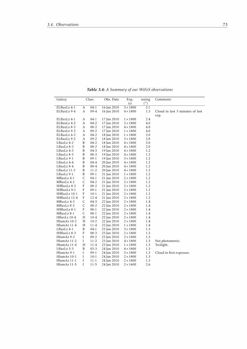
• The observing described in Section 3.4 were completed withthe help of those listed in Table 3.3.

• Section 4.4 is the combined work of myself and Max Malacari,an undergraduate intern. We worked closely together, withI providing much of the guidance on how to approach theproblem, and Max implementing the algorithms I described.The measurements of clump sizes presented are his.

• At all points through this work, Karl Glazebrook and ChrisBlake, my thesis advisers, provided extensive suggestions,ideas, and support.

Many of these people are co-authors on relevant papers derived fromthis work.

1.3 Previously published work

Some sections of this thesis have already been published in the jour-nal Nature as “High star formation rates as the origin of turbulencein early and modern disk galaxies” (Green et al., 2010). This includes

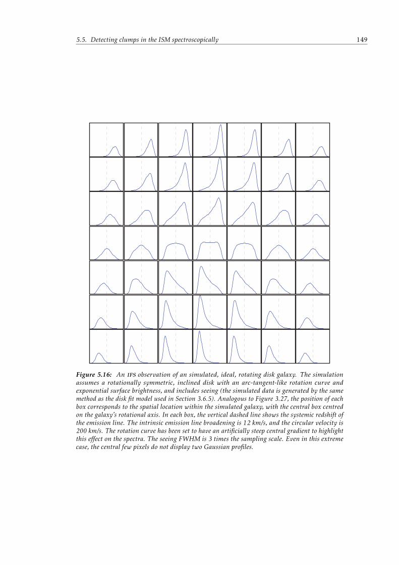
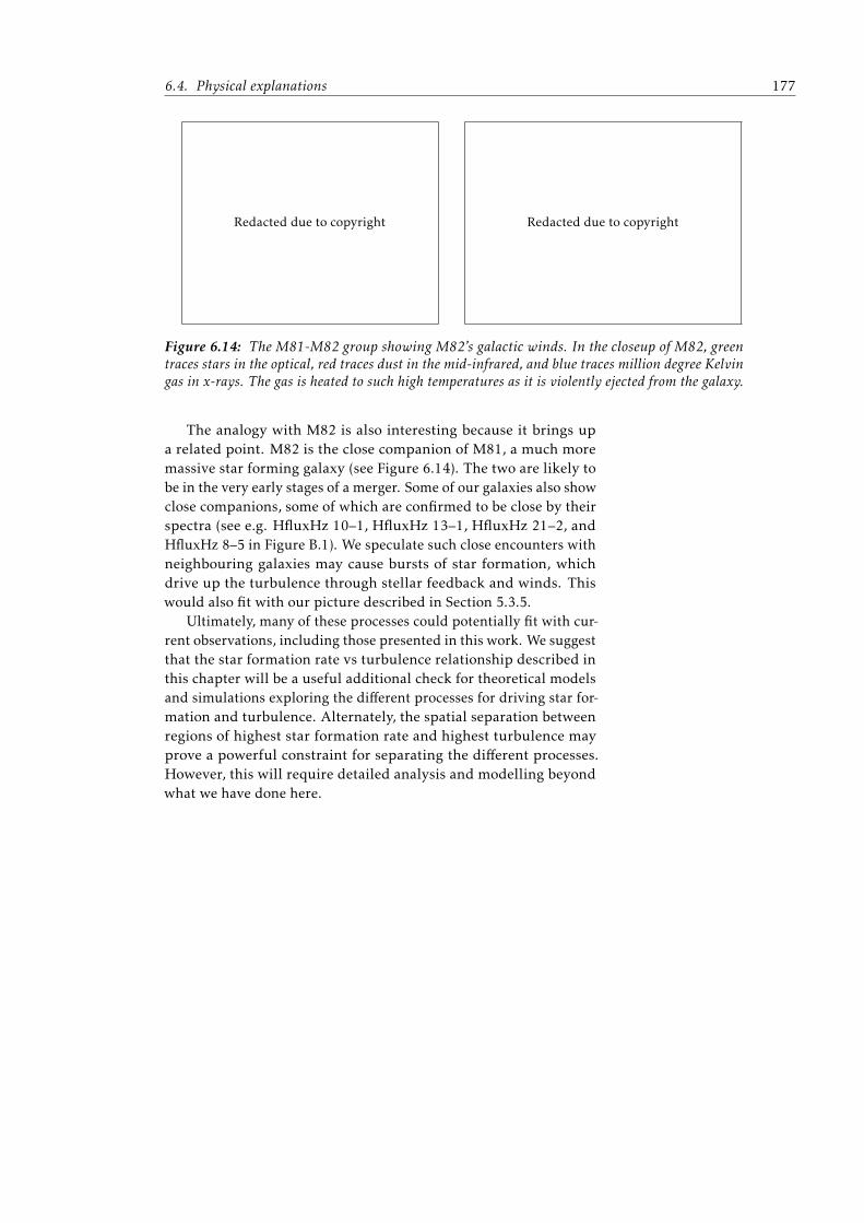
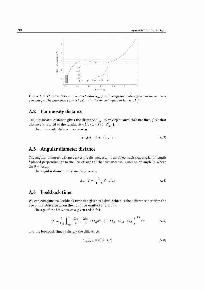
Redacted due to copyright

Figure 1.1: The cover ofthe 7 October issue of Na-ture featuring work pre-sented in this thesis. (Greenet al., 2010)

most of Chapter 6. That chapter includes additional data not pub-lished in the above work, and presents some physical explanationswhich could not be included in the tight word limits of Nature.

Additional data not presented in Green et al. (2010), and furtherinsights will be submitted for publication upon completion of thisthesis. That work includes the remaining sections of Chapter 6 notalready published. It also includes the star formation rates computedin Section 4.1.3, and brief overview of the spiral and WiFeS datareduction and analysis presented in Chapter 3.

A third paper is planned in collaboration with E. Wisnioski tofurther study star forming clumps at low- and high-redshift, andwill be an extension of the discussion in Section 4.4.

1.4 Brief plan of this thesis

Chapter 2 provides extensive background necessary for our discus-sion. First, it outlines our knowledge of star formation and starforming galaxies. In particular, it includes previous understandingabout the kinematics of star forming galaxies. Then, it describes theintegral field spectrograph, an important new instrument for study-ing galaxies, which this work will use extensively. Finally, it outlinesrecent results using these new instruments on the kinematics ofgalaxies both in the modern and earlier epochs.

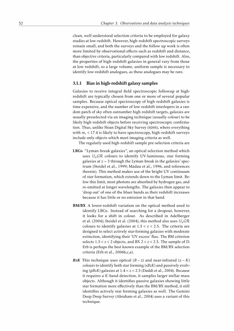
Chapter 3 details the observational data that makes up this thesis.It first explains how candidate galaxies for observation are identified,and summarises the characteristics of the selected galaxies. It definesthe observational procedures employed at each of the telescopes usedfor our observations. Finally, it specifies the data reduction steps foreach instrument, and the analysis steps common to all instruments.

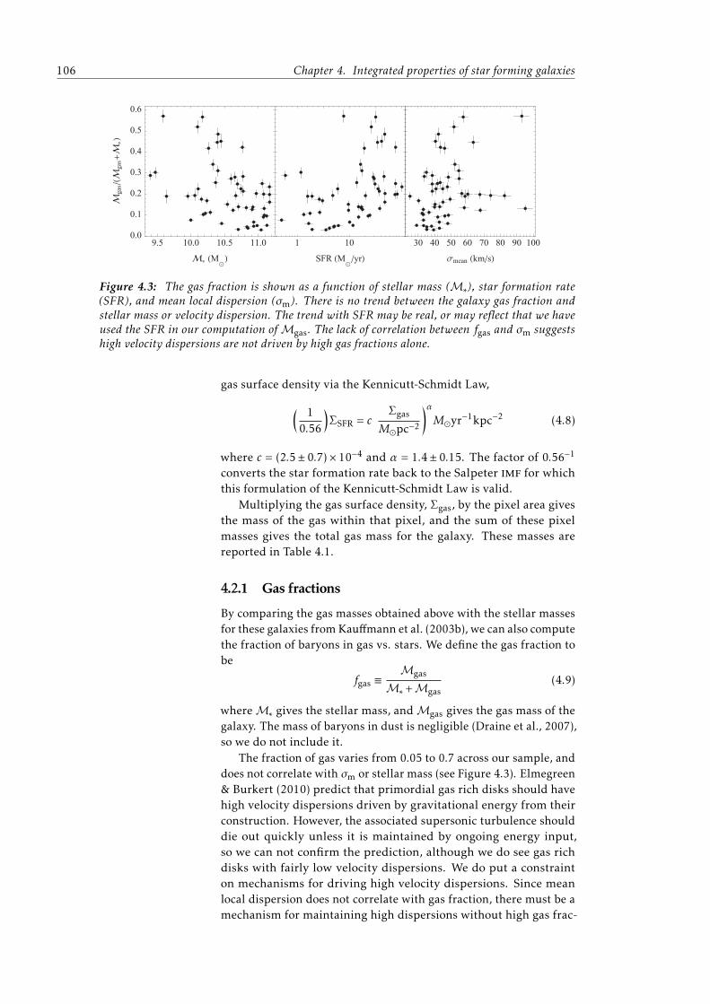
Chapter 4 covers the integrated properties of our sample. It mea-sures the Hα emission line luminosity, absorption from interstellar

4 Chapter 1. Introduction

dust, and star formation rates of these galaxies. It estimates the massfraction of gas within these galaxies, and explores the gas fraction’srelationship to other quantities. It then compares the quantitiesderived from this data with those derived from single fibre aperturedata to shed light on the effects of different size apertures on galaxyproperties. Finally, it presents measurements of the sizes of clumpsin very high resolution imaging of one galaxy in the sample.

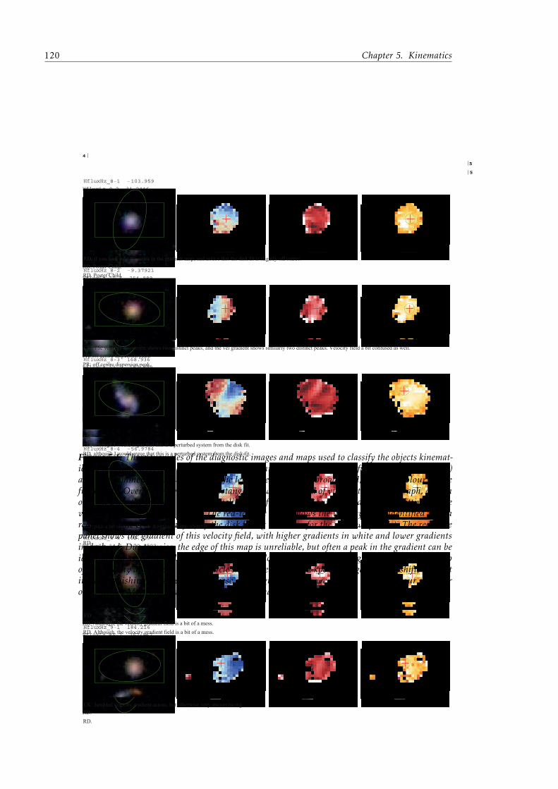
Chapter 5 explores the kinematics of star forming gas withinthese galaxies. First, it enumerates a kinematic classification schemefor the sample. The galaxies are divided into these classifications,and some other possible schemes are considered. Then, it focuseson the velocity dispersion of these galaxies, and the different waysof measuring it. It explores what kinematic information can berecovered from the shape of the emission line in individual, spatiallyunresolved spectra of the galaxies observed. It presents the Tully-Fisher relation for our sample, and compares it with other measuresof this relation. Finally, it discusses the stability of these galaxiesbased on our understanding of their kinematics.

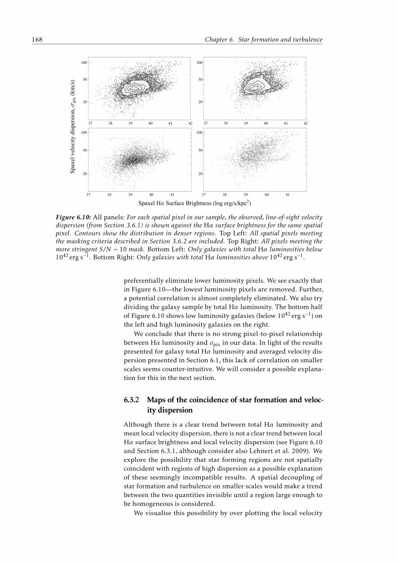
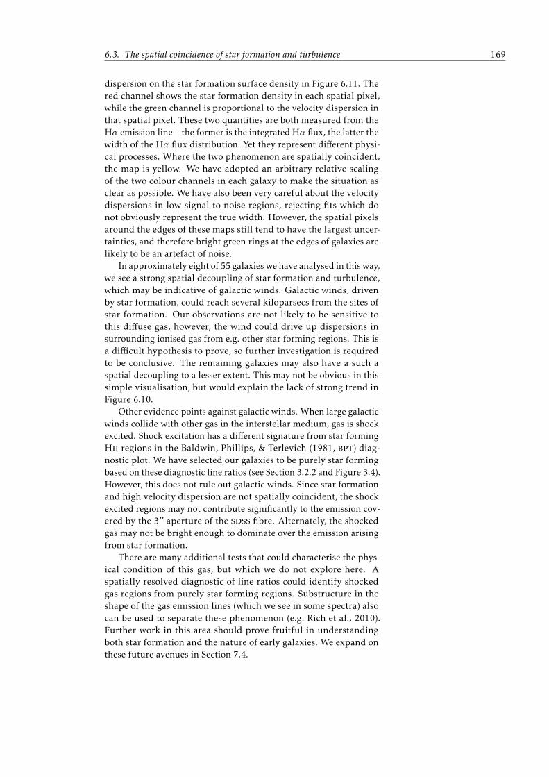
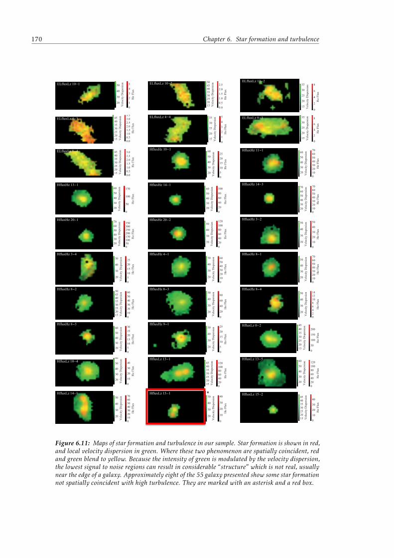
Chapter 6 presents the relationship between star formation andvelocity dispersion seen in galaxies across cosmic time. It first de-tails the data used and shows that the correlation is robust againstdifferences in the details of measurement. Next, it argues the linkbetween these two quantities is fundamental, and not a manifesta-tion of another relationship with other physical parameters of thegalaxies. The chapter establishes the spatial relationship betweenregions of high star formation and regions of high turbulence, whichalso explains why some previous attempts to measure this relationhave been less successful. Finally, it provides an extensive discussionof possible physical mechanisms driving this empirical relationship.

Finally, Chapter 7 reviews the results presented in this thesis, andsuggests avenues of future research. In particular it clarifies that newinstruments and techniques have not affected already establishedresults on galaxy evolution. It also brings together the evidence thatobjects with the same properties as high-redshift galaxies still existtoday. The chapter finishes with several potential future projects.

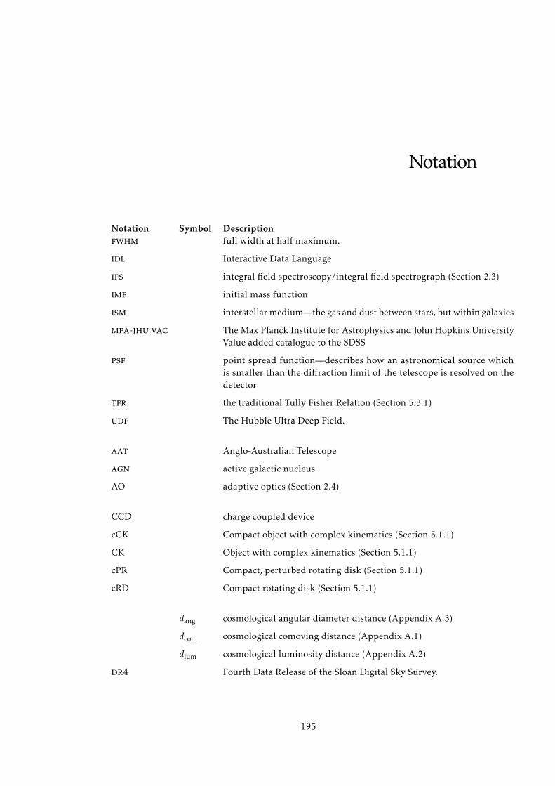
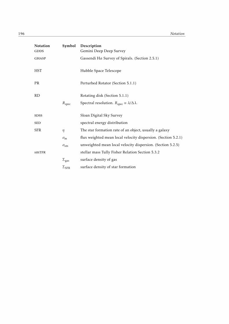
Throughout this thesis, we will use several acronyms, abbrevi-ations and symbols. I will endeavor to remind the reader of theirmeaning whenever it may not be clear. Also, a list of these can befound on page 195. In a few cases, particularly for the names ofinstruments, the acronym is better known in common usage thanwhat it stands for, and therefore we use the acronym exclusivelyexcept when introducing the instrument. The mathematical symbolsand their meanings are consistent throughout the document, and themore common ones are also listed in the glossary on page 195. Whenreferring to another work, we endeavor to make clear the differencesin notation for quantities we discuss.

Most of this thesis is set in the present tense, and will use “we”to include myself and the reader as together we work through theanalysis and discussion presented. For the description of the obser-vations, I will use the past tense, and “we” will describe the teamconducting the observations, which usually included myself.


Kurt L. Adelberger 2Background

We begin by reviewing the current understanding of galaxy evolutionand the recent developments relevant to our goals. The evolutionof galaxies is an extremely complex problem, one which has beenof interest to astronomers even before galaxies were identified asdistinct from the Milky Way. The tools available to study galaxiesare extensive, and have become increasingly complex and capable.We wish to review, at least briefly, the history of the problem as wellas the tools brought to bear on it. Our review focuses on the aspectsmost relevant to the rest of this work: star forming galaxies, integralfield spectrographs, and the most recent work combining the two.This review is necessarily brief, and more information on the varioustopics is available in the references mentioned. After this chapter,the reader should understand the context in which this work is set,and the motivations for the work.

We begin in Section 2.1 with a wide ranging discussion of galaxyevolution, especially evolution in star forming galaxies. It toucheson several issues relevant to later chapters, and we will refer to itregularly. Much of this section will be familiar to astronomers. Sec-tion 2.2 focuses more specifically on the kinematics of star forminggalaxies, and the key kinematic relationship for star forming disks:the Tully Fisher Relation. This information should be familiar toanyone studying galaxies. Section 2.3 describes an astronomical cam-era in which each spatial resolution element of the image includesa whole spectrum: the integral field spectrograph. It includes de-scriptions of most of the different techniques used to achieve integralfield spectroscopy, as well as some of the earliest results. Section 2.4briefly explains the advantages and shortcomings of adaptive opticswhen used with integral field spectrographs. Section 2.5 summarisesthe recent works on galaxies at low redshift (z < 0.3) using integralfield spectroscopy. Section 2.6 provides a brief synopsis of individualworks employing integral field spectroscopy on galaxies at higherredshifts. It also summarises together the kinematic results of the

5

6 Chapter 2. Background

various works. Section 2.7 concludes the chapter with a sketch of themotivation for this work in the context provided.

2.1 Star forming galaxies and their evolution

Galaxies are large collections of stars, gas and dust, all gravitationallybound together and embedded within a dark matter halo (for adiscussion of “What is a galaxy” see Forbes & Kroupa, 2011, andreferences therein). Stars are probably the best studied constituent,but not necessarily the most significant1. They primarily form withingalaxies, although not all galaxies host significant star formation. Thepresence of star formation is often the most important distinguishingcharacteristic of a galaxy. Other defining characteristics are usuallytheir morphology, or shape; and their spectral type, or colour.

Galaxy mass assembly is fundamentally about gravity and starformation.2 The evolution of galaxies is tightly linked to where, how,and when stars form. The processes of star formation, their evolution,and their often highly explosive destruction all contribute hugeamounts of energy to the galaxies they populate, yet star formationis also not well understood, even though it is often studied. Anystudy of galaxy evolution will necessarily have to probe, and likelyimprove, our understanding of star formation.

2.1.1 What is a star forming galaxy?

The presence of significant star formation is a galaxy’s most impor-tant characteristic. Galaxies without star formation are known aspassive or quiescent. Because the presence of star formation has sucha great impact on a galaxy’s properties, there are many characteris-tics that can distinguish ‘star forming’ from ‘passive’ galaxies: themorphology (or shape); and the colour of the galaxy are two suchcommon characteristics; of course the star formation rate itself canalso be used to divide galaxies. Although these classification methodsmay not agree for individual galaxies, they reflect the importance ofstar formation in the evolution of galaxies. We will discuss some ofthese characteristics at length in this work.

Morphology or shape

Star forming galaxies generally appear to be thin disks, at least inthe modern Universe. The Milky Way is one such example, althoughthere are no “birds eye” views of it (Carroll & Ostlie, 1996). Thesedisks often have distinctive spiral arms. When the spiral arms areparticularly symetric and well defined, the galaxy is sometimes re-ferred to as a “grand design spiral” (Elmegreen & Elmegreen, 1982).Star forming galaxies are often referred to synonymously as “spiral”or “disk” galaxies.

1By mass, gas sometimes dominates over stars.2Dark matter mass assembly creates halos of dark matter, but not galaxies com-

posed of stars. I am not suggesting that dark matter halo assembly is not necessaryand important to galaxy formation, but instead that it is not sufficient for galaxyformation.

2.1. Star forming galaxies and their evolution 7

10.0 10.5 11.0 11.5

-2

-1

0

1

Mass Hlog M

L

Star

Form

atio

nR

ateHlo

gM

yr-

1 L

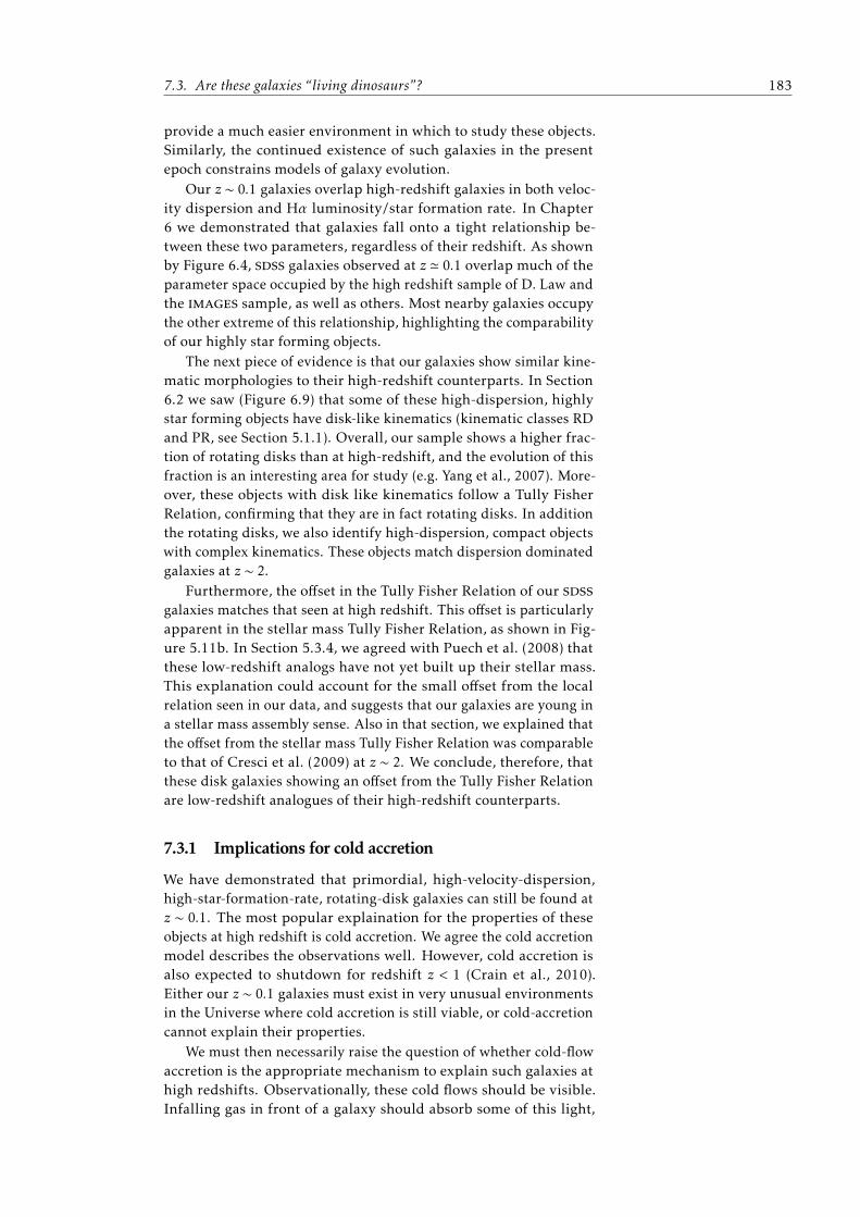
Figure 2.1: The contours show the number of galaxies from the SloanDigital Sky Survey in star formation rate and mass space (Brinchmannet al., 2004; Kauffmann et al., 2003b). Although there is some overlap,there are clearly two populations of galaxies represented.

On the other hand, passive galaxies tend to be more ellipticalor even spheroidal by comparison. They rarely have any featuresmarring their otherwise fuzzy appearance. As with spirals and disks,elliptical galaxies are often considered synonymous to describe pas-sive galaxies. Small galaxies at low-redshift often fit into neither ofthese morphological categories but are usually star forming. Theseare called dwarfs3.

Colour

Bluer galaxies tend to be star forming, while redder galaxies tendto be passive (Carroll & Ostlie, 1996). Galaxy colour is usually mea-sured by finding the difference between two broad-band magnitudes.The colour bimodality of galaxies reflects the underlying shape ofthe galaxy’s spectrum: hotter, short lived stars are bluer and brighter,dominating the galaxy’s total or bolometric luminosity during andshortly after star formation; cooler, longer-lived stars are redder andfainter, dominating the bolometric luminosity in passive galaxiesafter the bluer stars have died out.

Star formation rate

The best, but often not the simplest, way to classify galaxies as starforming or passive is to measure their star formation rate. As wehave already suggested, galaxies show a strong bifurcation in thisparameter (see Figure 2.1). However, the measurement of star for-mation rate generally requires more complex observations than areneeded to measure colour or morphology, as we’ll see later.

Complications to classification

Although morphology, colour, star formation rate and other criteriaoften easily divide the population of galaxies into two categories,these categorisations are not always consistent with star forming and

3Many dwarf galaxies are usually called dwarfs, not dwarves.



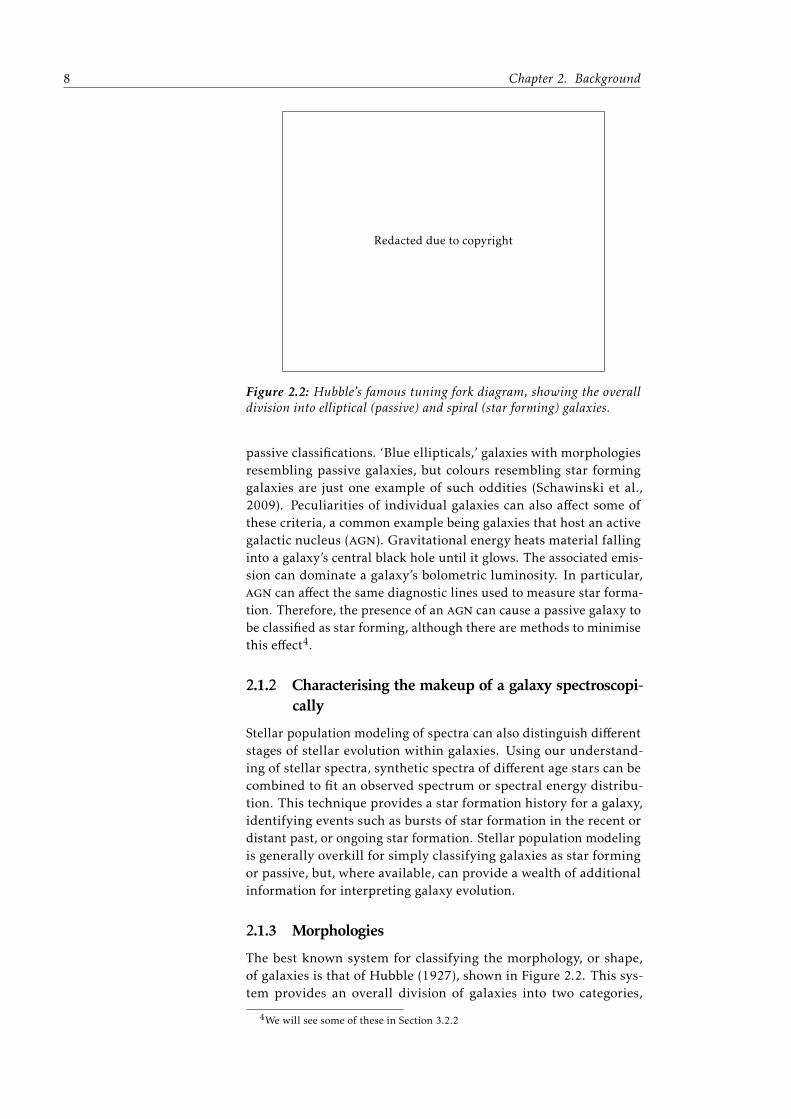
Figure 2.2: Hubble’s famous tuning fork diagram, showing the overalldivision into elliptical (passive) and spiral (star forming) galaxies.

passive classifications. ‘Blue ellipticals,’ galaxies with morphologiesresembling passive galaxies, but colours resembling star forminggalaxies are just one example of such oddities (Schawinski et al.,2009). Peculiarities of individual galaxies can also affect some ofthese criteria, a common example being galaxies that host an activegalactic nucleus (agn). Gravitational energy heats material fallinginto a galaxy’s central black hole until it glows. The associated emis-sion can dominate a galaxy’s bolometric luminosity. In particular,agn can affect the same diagnostic lines used to measure star forma-tion. Therefore, the presence of an agn can cause a passive galaxy tobe classified as star forming, although there are methods to minimisethis effect4.

2.1.2 Characterising the makeup of a galaxy spectroscopi-cally

Stellar population modeling of spectra can also distinguish differentstages of stellar evolution within galaxies. Using our understand-ing of stellar spectra, synthetic spectra of different age stars can becombined to fit an observed spectrum or spectral energy distribu-tion. This technique provides a star formation history for a galaxy,identifying events such as bursts of star formation in the recent ordistant past, or ongoing star formation. Stellar population modelingis generally overkill for simply classifying galaxies as star formingor passive, but, where available, can provide a wealth of additionalinformation for interpreting galaxy evolution.

2.1.3 Morphologies

The best known system for classifying the morphology, or shape,of galaxies is that of Hubble (1927), shown in Figure 2.2. This sys-tem provides an overall division of galaxies into two categories,

4We will see some of these in Section 3.2.2



Figure 2.3: Morphologies of galaxies from the Hubble Ultra Deep Field(udf). These are i775 band images showing “chains,” “clump clusters,”“doubles,” “tadpoles,” “spirals,” and “ellipticals” (Elmegreen et al., 2005,columns from left to right). These objects, seemingly typical among earlygalaxies, contrast with typical modern galaxy morphologies.

spirals and ellipticals. Elliptical galaxies have smooth light distri-butions, snd shapes varying from spheroidal (round) to lenticuar(disk shaped). Spiral galaxies have much more structure, displayingvarying numbers of spiral arms, and possibly a bar structure in thecentre. Generally, spirals are star forming, and ellipticals passive inour simple bifurcation (Section 2.1.1), although there are now studiesshowing exceptions to this rule (Schawinski et al., 2009).

Despite its popularity, identifying the Hubble type of a galaxy stillgenerally requires inspection of its optical image by eye. Therefore,it is inefficient to classify a large number of galaxies in this way.Efforts with many volunteers from the general public have beenhighly successful, albeit with a simplified Hubble sequence (Lintottet al., 2008). Major samples have also been classified by professionalastronomers (Nair & Abraham, 2010).

At high-redshift, however, the Hubble classification proves insuf-ficient to describe the plethora of galaxy shapes seen. The extremelydeep optical imaging in the Hubble Ultra Deep Field (udf) containsmany such objects (Beckwith et al., 2006). Some of these are repro-duced in Figure 2.3. Elmegreen et al. (2005) classified these objectsas “clump clusters”, “chains”, “doubles”, “tadpoles”, “spirals” and“ellipticals”. Only the last two categories overlap with the HubbleClassification. Clump clusters and chain galaxies are likely just dif-ferent viewing angles onto the same objects (Elmegreen, Elmegreen,& Hirst, 2004). Even so, these unusual looking galaxies have manyarticles attempting to understand their position in the galaxy evo-lution puzzle (Bournaud, Elmegreen, & Martig, 2009; Elmegreen,Bournaud, & Elmegreen, 2008, and references therein).

The clump cluster and chain galaxies are probably large starforming clumps embedded in a faint rotating disk (Genzel et al.,2011). A disk shape is necessary if chain galaxies really are clumpclusters viewed on edge. It is likely such an object would be rotating,as rotation provides the angular momentum necessary to create and


maintain the disk. Elmegreen & Elmegreen (2006) show that thesedisks have a large scale height (1.0 ± 0.3kpc), typically 1/3rd ofthe galaxy’s radial exponential scale length. However, despite thisconsiderable thickness, a perpendicular disk velocity dispersion ofonly 14 km/s is necessary to maintain this thickness.

Given the above, a simple evolutionary progression can thenbe described. Clump clusters (or chains) slowly build up the diskin which they are embedded, while dynamical friction causes theclumps to migrate to the centre of the disk, ultimately forming theprecursor to modern bulges. Theoretical simulations agree well withsuch an interpretation (Elmegreen, Bournaud, & Elmegreen, 2008).Unfortunately, this picture does not clearly describe doubles andtadpoles. These could simply be objects late in this time line, whereonly a couple of clumps remain before ultimately merging togetherto form the single central clump, and the disk is simply to faint to bedetected with current observations. Despite this complication, themodel is otherwise quite interesting given the available data.

2.1.4 Where star formation occurs

Star formation occurs in collapsing clouds of hydrogen gas. The sizeand temperature of these clouds can vary significantly, and thereforeseveral different names are used to identify these regions, such asgiant molecular clouds, Bok globules and Hii regions. Giant molecu-lar clouds are massive (up to 106 M) clouds of molecular hydrogen(H2) at ∼ 20 K, and typically about 50pc in size. Bok globules arecomparatively small regions (only ∼ 1pc), with masses of 1–1000M,but much higher densities. At sites of star formation within theseclouds, the hottest stars ionize the surrounding hydrogen. These Hii

regions5 glow from the emission associated with the recombinationof the electrons and protons. The Hα emission line at 6563Å is typi-cally the brightest of these emission lines in the optical wavelengths.

Hα is the n = 3 to 2 quan-tum transition of the elec-tron around the protonwithin the atom, and isthe first of the Balmer se-ries of lines, each repre-senting transitions fromhigher states to the 2nd en-ergy level of the hydrogenatom.

Hii regions are initially contained within the larger molecularclouds, but the surrounding gas is usually dissipated rapidly, makingthe glowing ionised regions visible from the Earth. Because thehottest stars (O and B spectral types) are short lived, they only ionisethe surrounding gas for a few million years. Therefore, the presenceof Hα emission indicates very recent or ongoing star formation, andin fact Hα emission is one of the best instantaneous tracers of ongoingstar formation (Kennicutt, 1998a).

Star formation begins when a region of gas is no longer stableagainst collapse. Jeans developed a theoretical criteria for this sta-bility in 1902. His approach considered when an infinite, uniformdensity cloud of gas was no longer stable against minor perturba-tions in density. It is still used today. His criteria set the size andmass of star forming regions based on the environment of the sur-rounding gas. Another criteria was developed by Safronov (1960)and Toomre (1964). Toomre’s Q parameter defines the stability ofa rotating disk against fragmentation and collapse. Although these

5Hii is the ionised form of atomic hydrogen, while Hi is the neutral form of atomic

hydrogen.


provide a theoretical understanding of the stability of the region, itis often not clear how these stability criteria interact in real systems(e.g. Elmegreen & Burkert, 2010).

2.1.5 What we know about star formation in galaxies

Star formation is a very complex process upon which many otheraspects of our understanding of galaxy evolution necessarily rest.Observationally, we have been able to identify many empirical lawsdescribing the process. These include the Kennicutt-Schmidt law, cor-relations in the basic properties of star forming regions, the efficiencyof star formation, and the initial mass function of stars within a sin-gle region. On the other hand, computer models provide insight onwhat physical processes might give rise to these relationships. Thesemodels are limited, however, by the complexity of the problem—theyare unable to include all of the relevant physics. Although muchis still not known about the details of star formation, by makingassumptions that fit with observations, we can still make progress inunderstanding the evolution of galaxies.

The Kennicutt-Schmidt law describes our empirical understand-ing of the relationship of star formation to gas density. Originallyintroduced by Schmidt (1959), this law shows a tight correlationbetween the star formation surface density, ΣSFR and the gas surfacedensity Σgas:

ΣSFR = cΣgasα (2.1)

where c and α are constants. The gas surface density is typicallymeasured using radio observations of Hi or CO. The star formationrate surface density is usually measured with optical observationsof Hα emission. This simple law remains valid for more than fiveorders of magnitude in star formation rate, from quiescent galaxiesto the biggest star bursts, as shown in Figure 2.4 (Kennicutt, 1998b).

The initial mass function (imf) describes how stellar mass is di-vided among newly formed individual stars. The form of the imfwas characterised by Salpeter (1955). This has been updated severaltimes with more accurate measurements of the mass contributions oflow mass stars,M < 1M (e.g. Kroupa, 2001; Chabrier, 2003). Thereare also indications that the imf may vary depending on the envi-ronment of star formation (Hoversten & Glazebrook, 2007; Kroupa,2001; Meurer et al., 2009). However, there is still no good theoreticalexplanation for the physics behind the imf.

Observations show the efficiency of converting gas into star for-mation is small, perhaps only 1–2%. Yet numerical simulations havestruggled to restrain star formation to such small efficiencies. Tra-ditionally, the low efficiency is attributed to magnetic fields. Thesefields are both difficult to measure and to simulate, and, althoughtheoretically valid, may not be the real cause. Recent numerical workof Bate (2009) suggests that radiative feedback from newly formedstars may be more relevant to reducing efficiency.

Star formation is a hugely energetic process. The gravitational po-tential energy of the gas which forms stars must be released as the gascollapses. This energy, much of which escapes as radiation, will heatthe surrounding medium. The brightest stars, which have lifetimes



Figure 2.4: The Kennicutt-Schmidt Law is an empirical relationship between star formationrate density and gas mass for star forming galaxies. This compilation of data from Kennicutt(1998b) shows the tightness of the relationship over many orders of magnitude in both gas andstar formation surface density.


comparable to the timescales for star formation itself, emit signifi-cant ultraviolet radiation, which ionises and heats the surroundinghydrogen gas. The radiation and stellar winds eventually sweepaway remaining gas not incorporated into stars. Finally, supernovaexplosions, which start only a few million years after star formationbegins, also inject vast quantities of energy into the surroundingmedium.

The rate of star formation with a galaxy or region can be deter-mined by several different methods. The very hot, but short livedspectral type O and B stars ionise the surrounding hydrogen withtheir UV radiation. When the electrons recombine with the protons,they emit light in several different narrow lines corresponding toquantum transitions within the hydrogen atom. Because these Oand B stars are short lived, only a few million years, the associatedionising radiation is indicative of very recent or ongoing star forma-tion. So the intensity of the narrow hydrogen emission lines can berelated to the star formation rate. The Balmer lines Hα and Hβ haveboth been calibrated as star formation indicators (Kennicutt, 1998a).These emission lines are often used as indicators of ‘instantaneous’star formation.

Alternately, the hot, short lived stars indicative of recent star for-mation are brightest in the UV. Measurements of the broadband UVluminosity have also been calibrated as star formation rate estimators(Kennicutt, 1998a). Because UV luminous stars contributing to thisluminosity have longer lifetimes than the ionising O and B stars, thisindicator can indicate recent star formation as well as instantaneousstar formation (but it is impossible to differentiate between themwith UV observations alone.)

Interstellar dust can affect these star formation rate indicators.Dust absorbs light at short wavelengths, and eventually re-emits ita longer wavelengths as a black body. Therefore, it is necessary tocharacterise the quantity of dust affecting an observation, and correctfor it in estimates of the star formation rate. A more detailed reviewof this can be found in Osterbrock (1989).

Finally, the star formation rate can be measured by consideringthe spectral energy distribution of the galaxy. This requires measure-ments of the energy output of a region or galaxy in several widelyseparated broadband filters. These measurements are then comparedwith models based on libraries of stellar spectra and stellar lifetimesto determine the star formation rate in a process known as stellarpopulation modeling. Such modeling can also be used to infer thepresence of previous star formation, and even the full history ofstar formation within the region. The other methods of measuringstar formation rates are just simplified versions of stellar populationmodeling.

Even though star formation is a complex process, these complexi-ties can often be ignored. The process can often be represented verysimply with little change in the results when its details are not im-portant to the question being considered. In this thesis, we will oftenignore many of these complexities where they will not qualitativelyaffect our conclusions. We discuss places where this approach maynot be valid as we come to them.



Figure 2.5: The star formation history of the Universe. The star forma-tion density peaks around z = 2 or log10(1 + 2) = 0.48. This compilationis from Hopkins (2004) as presented in Zhu, Moustakas, & Blanton(2009). This relation was first noted by Lilly et al. (1996) and Madauet al. (1996).

2.1.6 Star formation in the context of galaxy evolution

Because we are now able to look back over a significant fraction ofthe age of the Universe, we expect to see the star formation propertiesof galaxies change with look-back time. These changes reflect bothevolution in the process of star formation itself, and in the galaxiesin which it occurs. The star formation rate density of the Universevaries with time. The properties of star forming galaxies, particularlymorphology, change as well. And, the environment of star formation,both within the galaxy, and of the galaxy itself, changes significantlyas the Universe evolves. Although these changes significantly com-plicate our picture of star forming galaxies, they help explain galaxyevolution.

The star formation rate volume density of the Universe has de-clined significantly in the past six billion years. This decline is shownby the ‘Madau’ plot of the space density of star formation againstredshift (Madau et al., 1996; Lilly et al., 1996). Figure 2.5 shows anupdated version of this diagram. The density seems to peak aroundz = 2, when the Universe was one-third its present age, and thendecline significantly to the present. The density at earlier times isless well constrained, but seems to decline slightly with further lookback. Because the density has evolved so strongly (a factor of ∼ 4),there is a great deal of interest in studying galaxies across this timespan to identify how they have changed.

One such important change of interest is the build up of the redsequence. As the rate of star formation in a galaxy declines, the itchanges from being “star forming” to “passive”. As short lived bluestars die out, the red stars remain, giving the galaxy a red colour.These red galaxies fall along the red sequence in a colour vs. magni-

2.2. Galaxy kinematics and the Tully Fisher Relation 15

tude plot. As the star formation rate density of the Universe declines,we might expect the red sequence to build up. The red sequenceis already in place by z ∼ 1.5 (e.g. McCarthy et al., 2004), but fur-ther buildup of stellar mass within galaxies (Puech et al., 2008), andchanges in the fraction of passive and star forming galaxies probablycontinue through today (e.g. Peng et al., 2010; Abraham et al., 2007).

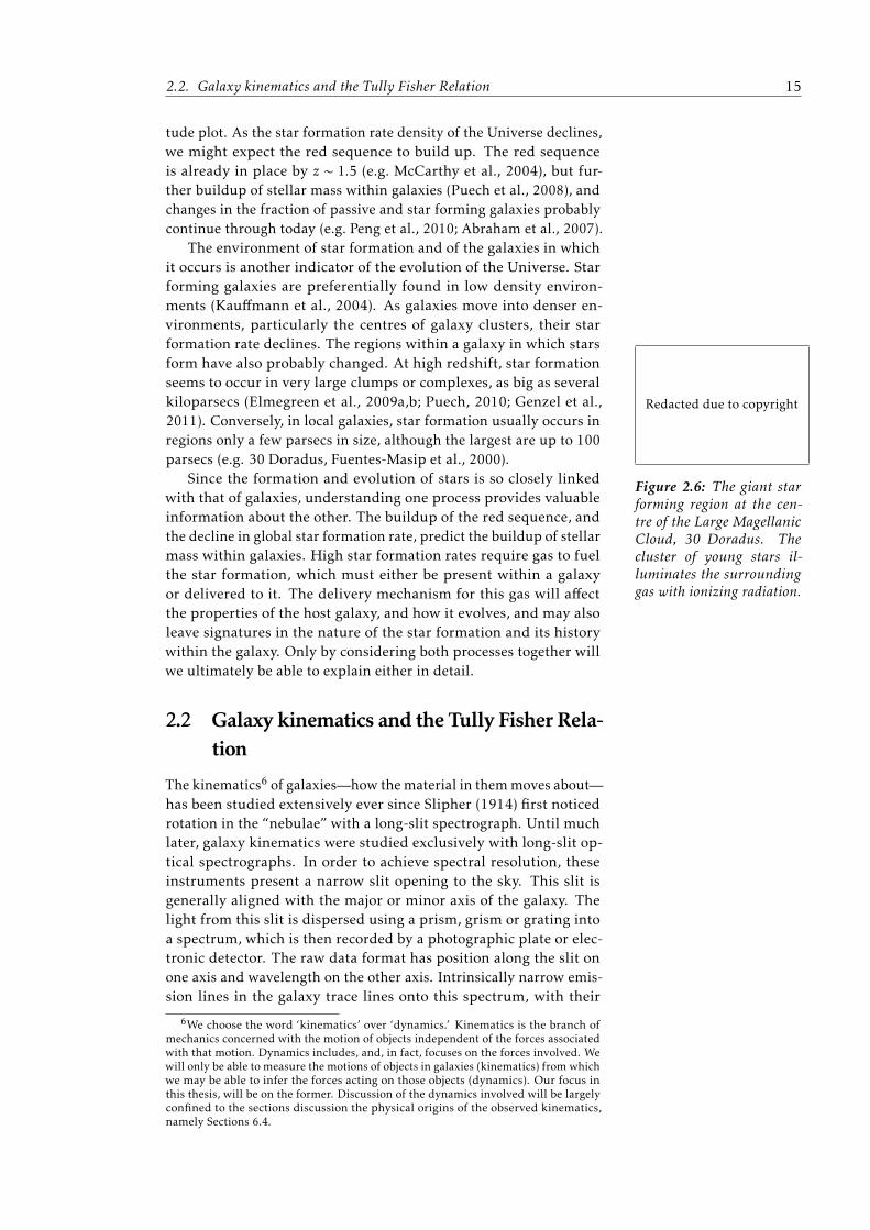
The environment of star formation and of the galaxies in whichit occurs is another indicator of the evolution of the Universe. Starforming galaxies are preferentially found in low density environ-ments (Kauffmann et al., 2004). As galaxies move into denser en-vironments, particularly the centres of galaxy clusters, their starformation rate declines. The regions within a galaxy in which starsform have also probably changed. At high redshift, star formationseems to occur in very large clumps or complexes, as big as severalkiloparsecs (Elmegreen et al., 2009a,b; Puech, 2010; Genzel et al.,2011). Conversely, in local galaxies, star formation usually occurs inregions only a few parsecs in size, although the largest are up to 100parsecs (e.g. 30 Doradus, Fuentes-Masip et al., 2000).


Figure 2.6: The giant starforming region at the cen-tre of the Large MagellanicCloud, 30 Doradus. Thecluster of young stars il-luminates the surroundinggas with ionizing radiation.

Since the formation and evolution of stars is so closely linkedwith that of galaxies, understanding one process provides valuableinformation about the other. The buildup of the red sequence, andthe decline in global star formation rate, predict the buildup of stellarmass within galaxies. High star formation rates require gas to fuelthe star formation, which must either be present within a galaxyor delivered to it. The delivery mechanism for this gas will affectthe properties of the host galaxy, and how it evolves, and may alsoleave signatures in the nature of the star formation and its historywithin the galaxy. Only by considering both processes together willwe ultimately be able to explain either in detail.

2.2 Galaxy kinematics and the Tully Fisher Rela-tion

The kinematics6 of galaxies—how the material in them moves about—has been studied extensively ever since Slipher (1914) first noticedrotation in the “nebulae” with a long-slit spectrograph. Until muchlater, galaxy kinematics were studied exclusively with long-slit op-tical spectrographs. In order to achieve spectral resolution, theseinstruments present a narrow slit opening to the sky. This slit isgenerally aligned with the major or minor axis of the galaxy. Thelight from this slit is dispersed using a prism, grism or grating intoa spectrum, which is then recorded by a photographic plate or elec-tronic detector. The raw data format has position along the slit onone axis and wavelength on the other axis. Intrinsically narrow emis-sion lines in the galaxy trace lines onto this spectrum, with their

6We choose the word ‘kinematics’ over ‘dynamics.’ Kinematics is the branch ofmechanics concerned with the motion of objects independent of the forces associatedwith that motion. Dynamics includes, and, in fact, focuses on the forces involved. Wewill only be able to measure the motions of objects in galaxies (kinematics) from whichwe may be able to infer the forces acting on those objects (dynamics). Our focus inthis thesis, will be on the former. Discussion of the dynamics involved will be largelyconfined to the sections discussion the physical origins of the observed kinematics,namely Sections 6.4.



Figure 2.7: The first spectral map published for any galaxy (Argyle, 1965). This map shows Hispectra across the 2d extent of Andromeda on the sky.

shape reflecting the relative velocity of material at the given position.When this shape is measured along the major axis, and corrected forthe inclination of the galaxy, it is known as a rotation curve.

Rotation curves covering the nuclear region of M31 were soonavailable using emission lines observed with long slit spectrographsThe dedication of the

astronomers undertakingthis early work is extraor-dinary, as shown by theexposure times involved:Pease took an 84 hour anda 79 hour integration withthe Mt Wilson 60” tele-scope.

(Pease, 1918). Later, work would extend the M31 rotation curve tothe outer region of the galaxy. These rotation curves raised questionsabout the mass distribution within galaxies: mass could not simplybe proportional to the light distribution if Newton’s laws of grav-ity were to be respected. However, difficulties in making accuratemeasurements of a galaxy’s rotation velocity at large radius madesubsequent analysis of the problem alternate between different massdistribution models.

Early radio telescopes were able to probe the velocity distributionof neutral hydrogen to much greater galactocentric radii. Argyle(1965) recovered the first two dimensional velocity map of a galaxywith a radio telescope, shown in Figure 2.7. These observationsrevealed the flat part of the galaxy’s rotation curve more clearly—although at first this was attributed to side lobes in the radio beamand ignored. Radio observations using unresolved spectra, however,allowed the discovery of the relation between rotation speed and lu-minosity for spiral galaxies, which we discuss further in Section 2.2.3(Tully & Fisher, 1977).


Rotation curves can hide important kinematic details about agalaxy’s rotation. Most notable is the asymmetry of rotation betweenthe two sides of a galaxy. Position–velocity spectra from long-slitspectrographs can be used to estimate the fraction of asymmetricgalaxies to be 50% or more (e.g. Haynes et al., 1998). Much lesscommon, but still extant are systems where different components(gas, stars of different ages, etc.) are counter rotating (e.g. Bureau& Chung, 2006). However, the simplification of galaxies to rotatingdisks characterised by a rotation curve is a reasonable first approxi-mation.

Although the limited information available from a rotation curvecould often be overcome with a velocity map, instruments able toprovide such data in the optical wavelengths were slow to arrive.The only efficient way to record optical photons was on photographicplates, and instrument designs providing spatially resolved spectralinformation over two dimensions on such plates are complex. Opticalintegral field spectrographs, which we will describe in detail inSection 2.3, would not become widely available until the 1990s,and not popular until the 2000s. Long-slit spectrographs quicklybecame easy to use and build, with many dedicated data reductiontools, even before electronic computing, available and easy to use.Integral field spectrographs, conversely, were often very complex, orrequired combining many exposures. Data reduction was similarlycomplex, and often required a myriad of calibrations. The advantageof velocity maps of galaxies over long-slit rotation curves was oftenoutweighed by these difficulties.

Where integral field spectroscopy really comes into its own, how-ever, is for studies of high-redshift galaxies. By this time, thousandsof galaxy rotation curves were already available from work such asMathewson & Ford (1996). But the apparent size of galaxies quicklydiminishes with redshift, and newly discovered galaxies at z ∼ 1 andhigher are too small to be easily studied with traditional long-slitspectrographs.

When observing galaxies at high redshift with a long-slit spec-trograph, the first problem is simply to identify the major axis ofthe galaxy, the most interesting axis on which to align the slit. Aspectrum of the major axis will best probe a galaxy’s rotation curve.But the small size of the galaxy makes this difficult. Furthermore,the more complex morphologies noted at high redshift make identi-fying the most interesting kinematic axis difficult even without thesmall size and effects of atmospheric seeing. Second, even with theexcellent seeing of sites like Mauna Kea, these objects are often stillonly marginally resolved.

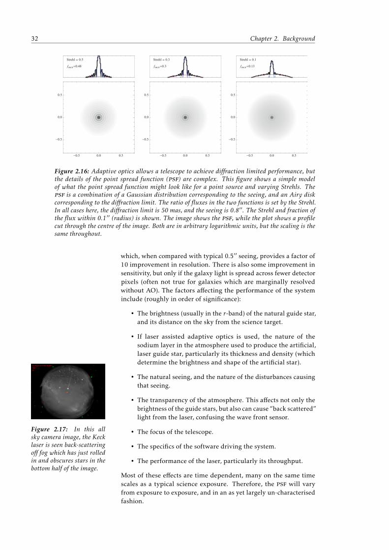
Adaptive optics (AO) solves this problem by providing near-diffraction limited performance in the near infrared bands, enablingresolved imaging of these galaxies. Atmospheric seeing results fromturbulence in the Earth’s atmosphere, and limits spatial resolutionavailable from the ground to typically 0.3′′ to 0.5′′ in the best loca-tions, regardless of telescope aperture. Integral field spectroscopyallows astronomers to both take advantage of diffraction limitedspatial resolution from adaptive optics and eliminate the need toidentify a galaxy’s major axis beforehand.


Redacted due to copyright Redacted due to copyright

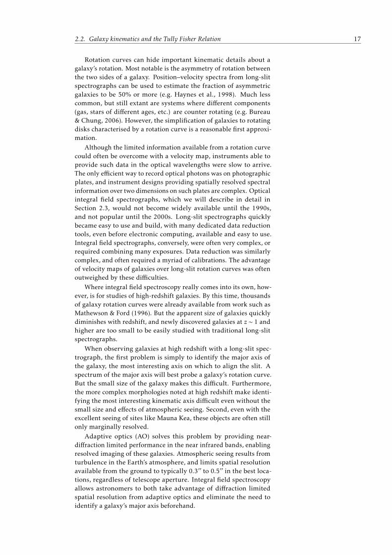
Figure 2.8: A comparison between a spiral and an elliptical galaxy.Andromeda (M31) on the left, is the closest galaxy to the Milky Way ofsimilar mass, and is a rotationally supported disk galaxy. On the right isM87, a giant elliptical galaxy. It is dispersion supported—the stars areon random, and often highly eccentric orbits around the galaxy centre.

An excellent review of galaxy kinematics and rotation curves instar forming galaxies is available in Sofue & Rubin (2001).

2.2.1 Kinematic morphologies

Galaxies can be classified by the motions of their stars and gas. Often,these motions also dictate the shape or morphology of the galaxy(Section 2.1.3). Thus these classifications can be thought of as kine-matic morphologies—describing the shape of the motions within thegalaxy. Unlike Hubble’s system for image morphologies, there aremany different classification systems for kinematic morphologies,none of which has been widely adopted. However, there are twogenerally accepted broad categories: dispersion supported systemsand rotationally supported systems.

Gravity pulls the material of a galaxy together, tending to want tomake it collapse, while the kinematics of the galaxy support it againstthis collapse. Physically, this support comes from the conservationof angular momentum—stars and gas orbit around their commonbarycentre. In rotationally supported galaxies, the primary kinematicbarycentre, like baryon, is

derived from the Greekword barý meaning heavy.

component is a rotating disk. The Milky Way and Andromeda areexcellent examples. These galaxies show a clear change in velocityacross their extent (unless they are viewed face on). For dispersionsupported systems, the stars (and gas, if present) orbit on randomlyoriented, and possibly highly eccentric orbits. An example is M87,a giant ball of stars with an extremely symmetric appearance. Inkinematic observations, these galaxies show a large line of sightvelocity dispersion, with a very smooth distribution. Figure 2.8shows Andromeda and M87 side by side.

These two broad categories generally reflect the difference be-tween star forming and passive galaxies. Because gas is able toradiate energy away, it tends to settle into a disk, the lowest energystate which conserves the overall angular momentum of the system.This gas then gives birth to stars which also orbit within this disk.As such, dispersion supported systems rarely have much gas, whileactively star forming systems tend to be rotationally supported diskswith gas. The morphological classifications into disks and ellipti-cals are often used synonymously with the kinematic morphologies


of rotationally supported and dispersion supported (respectively).However, even elliptical/dispersion supported galaxies often showsome global rotation (Emsellem et al., 2004).

Galaxies in the process of merging create a third general kine-matic category. Mergers are often easily recognised morphologicallyby their tidal tails—huge streams of stars strung about the surround-ing space by the gravitational interactions of the two galaxies. Kine-matically, mergers often present very confusing kinematics. Vestigesof rotationally supported disks from the progenitors may still beidentifiable, but otherwise the velocity field of the galaxy is often ajumble. Although mergers are often easily identified among localgalaxies, the much greater variation among high-redshift galaxiesmakes the systematic identification and distinction of mergers fromdispersion supported systems more difficult, particularly when com-pounded with reduced spatial resolution.

There are several more complex classifications for kinematic mor-phologies. Quantitatively, kinemetry defines a number reflecting thesymetry of the kinematics, and is useful for identifying and charac-terising rotating systems (Krajnović et al., 2006). Qualitative systemsare often developed for individual samples (e.g Epinat et al., 2009;Flores et al., 2006). The different systems typically identify disks asobjects which have centrally peaked velocity dispersion (resultingeither from unresolved velocity gradients at the centre of the disk, orfrom a central bulge, or both) and smooth velocity field characteristicof inclined perfect rotating disks. Non-disk objects may be classifiedas mergers, dispersion dominated systems, or otherwise dependingon the specific system used. None of these systems has yet beenwidely adopted, although kinemetry may be most common.

2.2.2 Kinematics of star formation

The kinematics of star formation really begins with Sir James Jeans,who defined a stability criteria for a cloud of gas against gravity(Jeans, 1902). A cloud of gas in interstellar space represents a balancebetween the internal kinetic energy (sometimes called ‘pressure’) ofthe cloud and the mutual gravitational attraction of all the particlesin the cloud. Jeans considered the mass and length scales on whicha small perturbation on the cloud would lead to the collapse of thecloud. The Jeans length is

λJ =πc2

sGρ0

(2.2)

where cs is the sound speed of the (ideal) gas, ρ0 is the mass density,and G is Newton’s gravitational constant. When a region is at leastthis size and density, it will begin to collapse under its own gravity.This can also be related to the minimum mass, the Jeans mass MJ, by

λJ =6GMJ

π2c2s

(2.3)

Once a region of this size begins to collapse, it will largely be infree fall. However, a cloud does not tend to collapse to form single



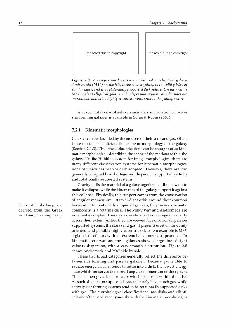
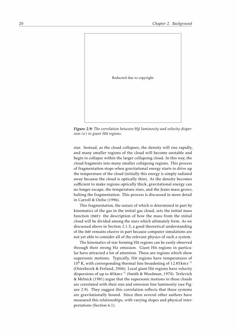
Figure 2.9: The correlation between Hβ luminosity and velocity disper-sion (σ ) in giant Hii regions.

star. Instead, as the cloud collapses, the density will rise rapidly,and many smaller regions of the cloud will become unstable andbegin to collapse within the larger collapsing cloud. In this way, thecloud fragments into many smaller collapsing regions. This processof fragmentation stops when gravitational energy starts to drive upthe temperature of the cloud (initially this energy is simply radiatedaway because the cloud is optically thin). As the density becomessufficient to make regions optically thick, gravitational energy canno longer escape, the temperature rises, and the Jeans mass grows,halting the fragmentation. This process is discussed in more detailin Carroll & Ostlie (1996).

This fragmentation, the nature of which is determined in part bykinematics of the gas in the initial gas cloud, sets the initial massfunction (imf): the description of how the mass from the initialcloud will be divided among the stars which ultimately form. As wediscussed above in Section 2.1.5, a good theoretical understandingof the imf remains elusive in part because computer simulations arenot yet able to consider all of the relevant physics of such a system.

The kinematics of star forming Hii regions can be easily observedthrough their strong Hα emission. Giant Hii regions in particu-lar have attracted a lot of attention. These are regions which showsupersonic motions. Typically, Hii regions have temperatures of104 K, with corresponding thermal line broadening of 12.85kms−1

(Osterbrock & Ferland, 2006). Local giant Hii regions have velocitydispersions of up to 40kms−1 (Smith & Weedman, 1970). Terlevich& Melnick (1981) argue that the supersonic motions in these cloudsare correlated with their size and emission line luminosity (see Fig-ure 2.9). They suggest this correlation reflects that these systemsare gravitationally bound. Since then several other authors havemeasured this relationships, with varying slopes and physical inter-pretations (Section 6.1).


Freshly formed stars also have important kinematic processesassociated with them. Protostars have highly energetic jets andwinds. All stars also produce stellar winds for most of their lifetimes,and for the largest stars, the energy in these winds integrated overthe life of the star can be as great as a supernova explosion (Mac Low& Klessen, 2004). In regions of ongoing star formation, supernovacan also play an important part in the kinematics of the region. Thefirst supernova will begin only a few million years after the firststars form. The primary kinematic component of a supernova isits expanding gas shell, blowing a bubble within the surroundingmedium.

Much of these details will become very important for interpretingthe results of this thesis. Chapter 6 in particular discusses this, andprovides more detail where necessary.

2.2.3 The Tully Fisher Relation

Perhaps the best known empirical correlations for star forming galax-ies is the Tully Fisher Relation. Discovered by Tully & Fisher (1977),it is widely interpreted (e.g. Mo, Mao, & White, 1998) as the relation-ship between a galaxy’s stellar mass (quantified by its luminosity)and the mass of the dark matter halo in which the galaxy has formed(quantified by the circular velocity, or really the angular momentumof the system). Originally, the circular velocities were determinedby measuring the velocity width of neutral hydrogen (Hi) spectra.The relationship was primarily developed as an aid to measuringdistances—measuring the circular velocity of a galaxy provided theabsolute luminosity.

Today, rotation velocities are often measured using long-slit op-tical spectrographs (e.g. Pizagno et al., 2007). Although it is stillcommon to use luminosity, the stellar mass Tully Fisher Relationhas less scatter, probably because it eliminates variation in the mass-to-light ratio of the galaxy (e.g. Pizagno et al., 2005; Bell & de Jong,2001; McGaugh et al., 2000). Despite ongoing study, there is nocomplete understanding of the relationship. In particular, the scatterin the relationship, which generally exceeds the measurement errorsignificantly in modern compilations, still lacks a widely acceptedexplanation (some ideas are given by e.g. Kannappan, Fabricant, &Franx, 2002). Unfortunately, the scatter in the relation is also difficultto compare, as most authors apply some kind of pruning to samplesused for Tully Fisher Relation analyses. Generally, objects whichare not clear rotating disks are removed. This may extend to remov-ing objects with asymmetric rotation curves as well. Unfortunately,methods differ, and are rarely applied objectively.

Early work to investigate the kinematics of high-redshift galaxiesstruggled with the resolution achievable on their small apparentsizes. Erb et al. (2004) presented slit spectra of the Hα emissionline for 13 objects in the northern Great Observatories Origins DeepSurvey field. They were able to identify spatially resolved shear inonly two galaxies, and placed an upper limit on the velocity sheerof the whole sample of 110kms−1. Erb et al. shows that even whenthe slit is aligned along the morphological major axis of the galaxy,


it may not be aligned along the kinematic axis, foreshadowing theneed for integral field spectroscopy7 to make accurate kinematicmeasurements of these complex objects.

Samples at z > 0.5 are only just becoming large enough to enablegood measurements of the Tully Fisher Relation at earlier times.Early constraints on possible evolution in the Tully Fisher Relationvary from none to at most 1 magnitude of luminosity evolution toz ∼ 1 (see references in Vogt et al., 1996). Flores et al. (2006) also findno evolution at z ' 0.6. However, Puech et al. (2008) find evolutionin an expanded sample based on the Flores et al. (2006) result. Usingthe large sins Survey8 sample, Cresci et al. (2009) find evolutionsimilar to that of Puech et al.. And Weiner et al. (2006b) find someevolution between z = 0.4 and 1.2 Tully Fisher Relations. Clearly,there is no consensus on whether or not the Tully Fisher Relationevolves.

Puech et al. (2008) suggest the evolution they observe in theTully Fisher Relation is due to the build up of stellar mass withoutchanging the halo circular velocity. As galaxies age and their starformation progresses, the stellar mass of the galaxy should grow.Gas already within the dark matter halo can be converted to stellarmass through star formation, while the mass of the halo itself wouldremain relatively constant. Any merging events would raise both themass of the dark matter halo and the stellar component.

Cresci et al. (2009) find good agreement between their observedevolution and galaxy simulations. They suggest the evolution isinstead a result of change in the angular momentum of the darkmatter halo. This evolution comes from contraction of the halo andthe baryons at its centre. In particular, a smooth, rapid accretion ofcold gas rather than merging events prevent abrupt changes in theangular momentum of the dark matter halo.

2.2.4 DEEP2 and S0.5

The deep2 Survey used the deimos instrument on Keck to observe alarge number of galaxies at z > 0.7 in four fields (Davis et al., 2003).In three of the fields, a colour cut in BRI bands allows a pre-selectionof targets likely to have z > 0.75. In the fourth field, the ExtendedGrowth Strip, no pre-selection is employed. For more extended ob-jects, the slits are tilted as much as 30 from the instrument positionangle to match the galaxy’s major axis and recover a rotation curve.

Of particular interest here is the modification to the Tully FisherRelation proposed by Weiner et al. (2006a). The modification is to thecircular velocity, and is designed to include the effect of non-circularmotions in supporting the galaxy against gravitational collapse. It isparametrised by

Sk =√kv2 + σ2 (2.4)

where σ quantifies the non-circular motions, v quantifies the rotationof the disk, and k defines the relative contribution to the galaxy’ssupport by each.

7We will discuss integral field spectroscopy in Section 2.3.8described in Section 2.6.1

2.3. Integral field spectroscopy 23

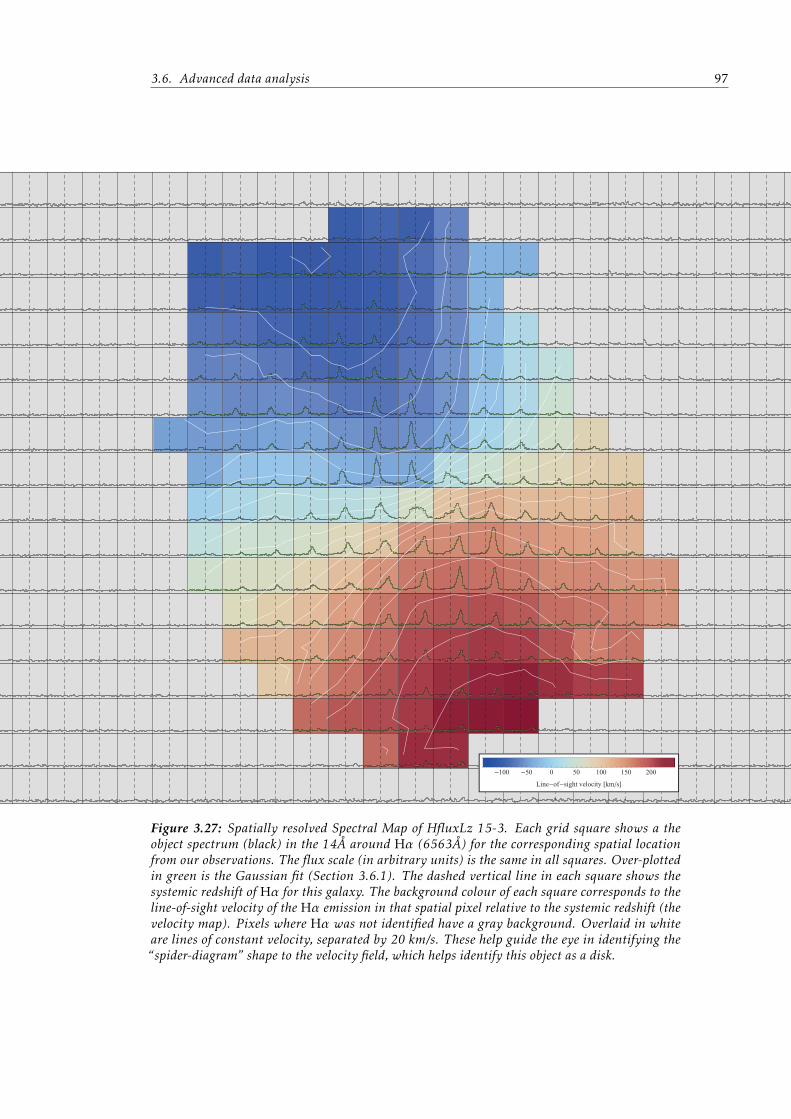
Figure 2.10: The integral field spectrograph can be thought of as a camera in which each pixelof the image actually includes a spectrum of the light in that pixel. Shown here is an image of agalaxy with a visualisation of the integral field spectroscopic data for that galaxy overlaid. Eachwhite square is a spatial pixel covering that area of the galaxy. Shown within the square is thespectrum in the neighbourhood of the Hα emission line. The circle shows a magnified view of thespectrum in one of these spatial pixels. A more technical rendition of this data for this same galaxyis shown in Figure 3.27 on page 97.

Kassin et al. (2007) show the Sk correction almost eliminatesoutliers in the Tully Fisher Relation. Cresci et al. (2009) also findthe Sk quantity to reduce the scatter in their Tully Fisher Relationat z ∼ 2, although even without this correction, their Tully FisherRelation shows remarkably little scatter9. Puech et al. (2010) alsofind that Sk reduces scatter, bringing all of their objects, includingthose with complex kinematics, onto the same relationship. Theynote, however, that the scatter in their z ' 0.6 sample remains largerthan typical local samples.

2.3 Integral field spectroscopy

Integral field spectroscopy (ifs) refers generally to observationswhich provide resolved spectroscopic information over a two-dimensionalfield of view on the sky, as illustrated in Figure 2.10. Although notnecessary, integral field spectrographs often provide a contiguousfield of view10, allowing an image on the sky to be constructed for aparticular wavelength or range of wavelengths. Hence the techniqueis sometimes referred to as imaging spectroscopy, but integral fieldspectrographs are distinct from imaging spectrographs such as the

9Cresci et al. attribute the small scatter to careful pruning.10Technically, the integral field refers only to a contiguous field. For various practical

reasons, “integral” field spectrographs do not provide a perfectly contiguous field.In some cases, they are even intentionally sparsely sampled, as in SparsePak (seeFigure 2.14 on page 29). However, even these non-contiguous field spectrographs arecommonly referred to as integral field spectrographs, so we do not make a distinction.


Low Resolution Imaging Spectrograph on Keck (LRIS), which pro-vide either imaging or spectroscopy, but not both simultaneously forthe same wavelength range.

There are many distinct techniques for obtaining spatially re-solved spectroscopic information across two dimensions on the sky,which we will describe in the rest of this section, along with an earlyhistory of integral field spectroscopic work. The following two sec-tions will outline the current state of integral field spectroscopicwork at low (Section 2.5) and high (Section 2.6) redshift.

2.3.1 Types of integral field spectroscopy

Scanning Fabry-Perot

The most common early integral field spectroscopic technique in-volves coupling a scanning Fabry-Perot (étalon) cavity to an imagingcamera. The Fabry-Perot is set to pass a particular wavelength (ac-tually a very narrow wave band), and an exposure is taken with thecamera, and then the Fabry-Perot is advanced to the next wavelengthstep and the process repeated to build up a series of images of theobject at each wavelength.

Fabry-Perot methods are necessarily slow. The Fabry-Perot cavitycan only pass one wavelength of light at a time—other wavelengthsare lost. A final exposure length of T seconds will require ' nTseconds to acquire, where the number of sub-exposures required isthe wavelength range divided by the desired resolution, n = ∆λ/δλ.No multiplexing across wavelength is generally possible. This meansthat the wavelength range chosen is tightly constrained around aspectroscopic feature of interest, although in theory multiple disjointsections of spectrum could be scanned (i.e. a narrow range aroundseveral emission lines). The main advantage over some other options,however, is the large field of view possible. This is generally limitedonly by the size of the detector.

Modern scanning Fabry-Perot integral field spectrographs usephoton counting detectors. Although sometimes used as well, ccdshave significant read out times and read noise, which are severelycompounded in the many exposures necessary to build up the spec-tral dimension. Image Photon Counting Systems, which detect in-dividual photons in real time, provide zero read noise and instanta-neous readout at the expense of greatly reduced quantum efficiency(Jenkins, 1987). The instantaneous readout is a particular advantage,as the Fabry-Perot cavity can be scanned across the wavelength rangerelatively quickly, with the process repeated many times to buildup a single 3d data cube. This reduces the impact of changing at-mospheric conditions systematically affecting the observation as afunction of wavelength. Despite the reduced efficiency of photoncounters, the advantages outweigh this shortcoming.

Even with these difficulties, Fabry-Perot systems still provide thebest system for contiguous coverage of a large area on the sky. Theyare particularly effective for surveys of nearby galaxies, where thecomparative brightness of the source can overcome some of the inef-ficiencies in the system. Scanning Fabry-Perot ifs was employed byTully (1974) to observe M51, and is used in the ghasp instrument on



Figure 2.11: A diagram of a Fourier transform imaging spectrograph.Light is fed from the focus of the telescope at the input. L1 collimates thebeam. The light then passes through a beam splitter, BSCA and travelsalong the two arms of the Michelson interferometer. The interferometeris “offset,” so the light returns from the end mirrors RR1 and RR2 alonga different path. RR2 can be translated to change the relative lengths ofthe two arms. Light is combined interferometrically at the second beamsplitter, BSCB. The light then exits the spectrograph via a filter, NBF, anda focusing lens L2 before reaching the detector D1. The second outputport is not shown, but would extend from the top of BSCB in the diagram,with the same filter, lens and detector setup.

the 1.93m telescope at the Observatoire de Haute-Provence (Garridoet al., 2002), both of which we discuss in this thesis.

Fourier transform imaging

A Fourier transform imaging spectrograph uses a Michelson inter-ferometer to measure the Fourier transform of the spectrum at eachspatial location. This interferogram can then be inverted into anormal spectrum of the object. In the basic design (shown in Fig-ure 2.11), light from the focus is collimated, and fed into an offsetMichelson interferometer. The two outputs of the interferometerare then refocused and imaged to produce a single measurementof the Fourier transform of the object’s spectrum, with each pixelcorresponding to that position on the sky. Changing the length ofone arm of the interferometer changes the sampling position of theFourier transform of the spectrum. By stepping the length of thearm and taking an exposure at each step, the full Fourier transformof the spectrum can be built up. A good diagram of the typical dataacquisition process is shown in Figure 1 of Drissen et al. (2008).

Perhaps the greatest advantage of Fourier transform imaging isin the large range of resolutions achievable with a single instrument.Effectively the number of times the Fourier spectrum is sampledsets the resolution of the final data cube. It can be sampled onceto produce just an image on the sky, or it can be sampled manytimes to produce a high resolution spectrum. The SpIOMM FourierTransform Imager has demonstrated resolution ranges of R = 1 to25,000 (Drissen et al., 2010).

Fourier transform imaging spectrographs are similar to Fabry-Perot systems in that they use an interferometer and require manyexposures to build up the final datacube. The read noise of the detec-


tor can be very important because it must be read many times overthe course of an observation. However, Fourier transform imagingsystems achieve higher throughput, as all of the photons from thesource are recorded in each frame, rather than just those belongingto a particular wavelength channel. While the overall efficiency ofthe Fabry-Perot approach is divided by the number of wavelengthchannels of the final data cube, the Fourier Transform approach doesnot suffer this inefficiency.

Unlike other approaches described here, the photon shot noisefrom the entire spectrum contributes to the noise at each spectralposition in Fourier Transform Imaging. Photons from the entirewavelength range of interest contribute to the Fourier transformspectrum at each sample, so they all contribute to the shot noise. Forpurely emission line targets, such as nebulae, this has little impacton the signal-to-noise of the observation. But for objects with sig-nificant continuum emission, such as stars, and early type galaxies,this can significantly affect the signal-to-noise of individual emissionor absorption line measurements. This problem can be mediated byincluding a pass-band filter, which brackets the particular area ofinterest. Potentially, even filters with multiple notches around par-ticular areas of interest could be used to prevent unneeded photonsfrom contributing to the shot noise.

Lenslet pupil arrays

Lenslet pupil spectrographs consist of a contiguous array of lenslets,which each focus light from the local region into a small pupil, whichis then dispersed with a grating or grism into a spectrum and imagedonto a detector (see Figure 2.12). By focusing the light to a smallspot, the spectra of neighbouring lenslets can be packed togetheron the detector. The location of the whole spectrum on the detectorcorresponds to the spatial location of the spectrum on the sky. Thegrid of the lenslets is rotated slightly from the wavelength dispersiondirection so spectra from neighbouring lenslets do not overlap oneanother. Unfortunately, such an approach makes the data reductioncomplex, particularly if the spectra are closely packed, as the indi-vidual spectra tend to interfere with one another. Additionally, thewavelength range available in a single exposure tends to be small,unless a significant reduction in spatial coverage is accepted.

This design is used in the osiris instrument on Keck and thesauron instrument (see Section 3.4.3 and 2.5.3). The design waschosen in particular for osiris because the optical path includes veryfew optical elements, and few moving parts, allowing the spectro-graph to reach diffraction limited performance and provide excellentlong term stability. Fewer optical elements reduce the contribution tothe global wavefront error11, allowing the instrument to achieve thevery high image quality needed to reach diffraction limited perfor-mance with adaptive optics12 on Keck. The lack of moving elementswithin the spectrograph and camera make the instrument very stable,critical as the calibration scans required for the data reduction take

11The wavefront error is the deviation of the wavefront from a perfect plane wave12Adaptive optics will be discussed in Section 2.4.



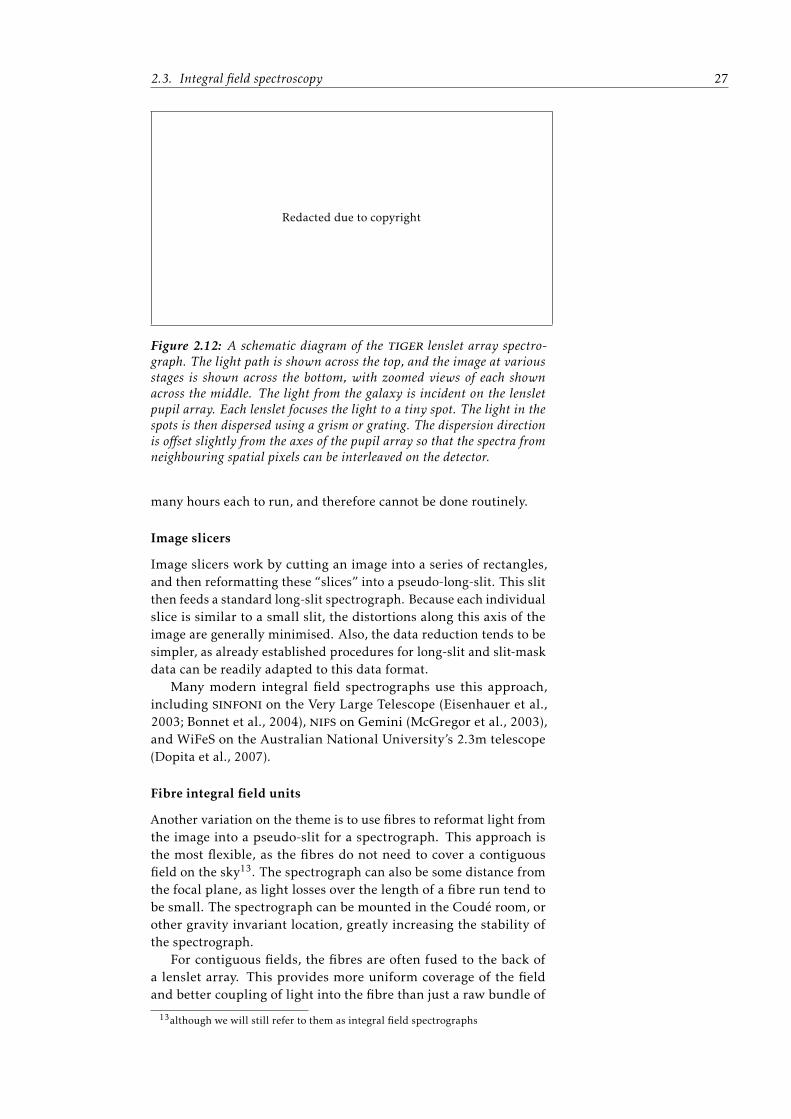
Figure 2.12: A schematic diagram of the tiger lenslet array spectro-graph. The light path is shown across the top, and the image at variousstages is shown across the bottom, with zoomed views of each shownacross the middle. The light from the galaxy is incident on the lensletpupil array. Each lenslet focuses the light to a tiny spot. The light in thespots is then dispersed using a grism or grating. The dispersion directionis offset slightly from the axes of the pupil array so that the spectra fromneighbouring spatial pixels can be interleaved on the detector.

many hours each to run, and therefore cannot be done routinely.

Image slicers

Image slicers work by cutting an image into a series of rectangles,and then reformatting these “slices” into a pseudo-long-slit. This slitthen feeds a standard long-slit spectrograph. Because each individualslice is similar to a small slit, the distortions along this axis of theimage are generally minimised. Also, the data reduction tends to besimpler, as already established procedures for long-slit and slit-maskdata can be readily adapted to this data format.

Many modern integral field spectrographs use this approach,including sinfoni on the Very Large Telescope (Eisenhauer et al.,2003; Bonnet et al., 2004), nifs on Gemini (McGregor et al., 2003),and WiFeS on the Australian National University’s 2.3m telescope(Dopita et al., 2007).

Fibre integral field units

Another variation on the theme is to use fibres to reformat light fromthe image into a pseudo-slit for a spectrograph. This approach isthe most flexible, as the fibres do not need to cover a contiguousfield on the sky13. The spectrograph can also be some distance fromthe focal plane, as light losses over the length of a fibre run tend tobe small. The spectrograph can be mounted in the Coudé room, orother gravity invariant location, greatly increasing the stability ofthe spectrograph.

For contiguous fields, the fibres are often fused to the back ofa lenslet array. This provides more uniform coverage of the fieldand better coupling of light into the fibre than just a raw bundle of

13although we will still refer to them as integral field spectrographs



Figure 2.13: A schematic diagram of an image slicer. The originalfield is shown at bottom right. This light is reflected by a slicing orstaircase mirror (S1) onto a series of individual pupil mirrors (S2). Thesemirrors bring the light into a pseudo-slit arrangement, with the imagenow reformatted as shown. This pseudo-slit can then be dispersed as in astandard long slit spectrograph.

fibres. The spatial pixels on the sky are then typically either squareor hexagonal. Square pixels in particular are extremely convenientfor data reduction and analysis tasks which have become stronglyoriented towards square, contiguous pixels. Both the spiral spectro-graph on the Anglo-Australian Telescope and the gmos integral fieldunit on Gemini use a lenslet array and fibres to feed a spectrographbuilt for other purposes (Sharp et al., 2006; Allington-Smith et al.,2002).

Non-contiguous fields are also possible, and can be very useful.Optical fibres are typically small (usually less than 4.5′′ on the sky),so a very large number would be necessary to provide contiguouscoverage of e.g. a nearby galaxy with large angular size. By spacingthe fibres, light from an object can be sparsely sampled, minimisingcost and scale of the spectrograph, while still providing a reasonablelevel of detail. The SparsePak ifs (Figure 2.14) on thewiyn14 tele-scope is well matched to probe nearby galaxies with ifs. The centralregion, were resolution is most critically is more densely sampledthan the outer region. A few fibres at larger radii from the galaxyprovide sky information for accurate sky subtraction.

Another variant of the non-contiguous field is to bundle fibrestogether into many groups. Each bundle can then be positioned ona galaxy, allowing resolved spectroscopy to be multiplexed acrossmany galaxies simultaneously. Such a multi-object ifs is comparable

14Wisconsin, Indiana, Yale and National Optical Astronomy Observatory (noao)telescope.



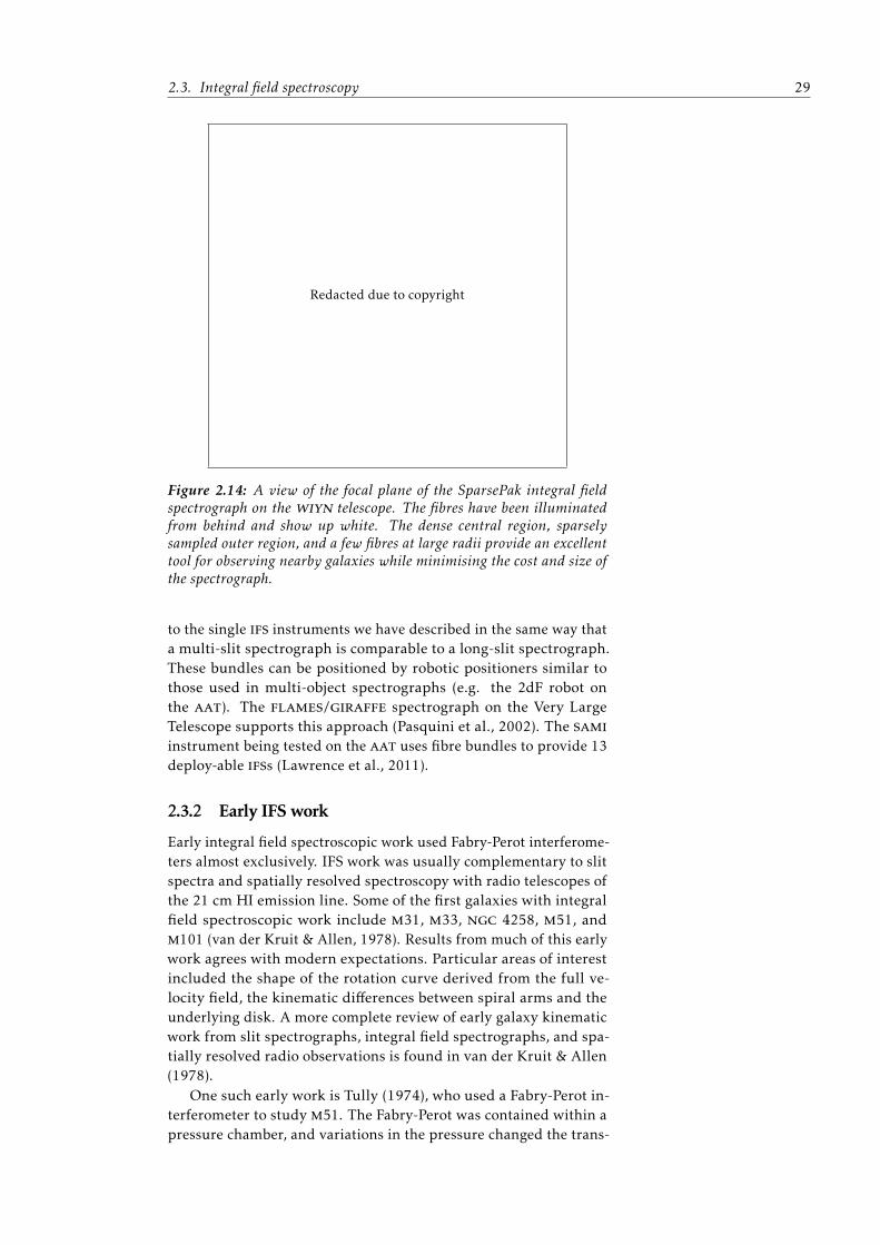
Figure 2.14: A view of the focal plane of the SparsePak integral fieldspectrograph on the wiyn telescope. The fibres have been illuminatedfrom behind and show up white. The dense central region, sparselysampled outer region, and a few fibres at large radii provide an excellenttool for observing nearby galaxies while minimising the cost and size ofthe spectrograph.

to the single ifs instruments we have described in the same way thata multi-slit spectrograph is comparable to a long-slit spectrograph.These bundles can be positioned by robotic positioners similar tothose used in multi-object spectrographs (e.g. the 2dF robot onthe aat). The flames/giraffe spectrograph on the Very LargeTelescope supports this approach (Pasquini et al., 2002). The samiinstrument being tested on the aat uses fibre bundles to provide 13deploy-able ifss (Lawrence et al., 2011).

2.3.2 Early IFS work

Early integral field spectroscopic work used Fabry-Perot interferome-ters almost exclusively. IFS work was usually complementary to slitspectra and spatially resolved spectroscopy with radio telescopes ofthe 21 cm HI emission line. Some of the first galaxies with integralfield spectroscopic work include m31, m33, ngc 4258, m51, andm101 (van der Kruit & Allen, 1978). Results from much of this earlywork agrees with modern expectations. Particular areas of interestincluded the shape of the rotation curve derived from the full ve-locity field, the kinematic differences between spiral arms and theunderlying disk. A more complete review of early galaxy kinematicwork from slit spectrographs, integral field spectrographs, and spa-tially resolved radio observations is found in van der Kruit & Allen(1978).

One such early work is Tully (1974), who used a Fabry-Perot in-terferometer to study m51. The Fabry-Perot was contained within apressure chamber, and variations in the pressure changed the trans-



Figure 2.15: A velocity map of m51 created using a scanning Fabry-Perot imaging technique(Tully, 1974).

mission wavelength of the interferometer. The light was then passedthrough an image intensifier before being recorded on photographicplates. With this purpose built instrument, Tully observed m51 toproduce the velocity map shown in Figure 2.15. Unfortunately, theinstrument began to disintegrate in the months the observationswere spread among, and much of the later data was discarded. Tullyprovided not only a highly accurate map of the velocity of m51, butalso measured the line-of-sight velocity dispersion to be ∼ 20 km/s.He noted that earlier observed deviations from pure disk like circularmotion in this object were probably erroneous, and resulted fromdifficulties in correctly interpreting the Fabry-Perot interferograms.Interestingly, this work was Brent Tully’s doctoral thesis.

Significant advances in integral field spectroscopy would takesome time, however. The increasing use of glass fibres to reformatlight from the sky for a slit spectrograph in the 1990’s led to theintroduction of several integral field spectrographs. A very earlyattempt using fibres to reformat a 2d field into a slit spectrograph isthat demonstrated for ngc 1365 on the Anglo-Australian Telescopewith the rgo spectrograph (Gray et al., 1982). This was followedby the spiral Phase A spectrograph, an earlier incarnation of thespiral we will discuss in Section 3.4.1 (Parry, Kenworthy, & Taylor,1997). hexaflex on the William Herschel Telescope was possiblythe first modern, regular use integral field spectrograph (Rasillaet al., 1990). The Max-Planck-Institut für extraterrestische Physik’s3d instrument provided near-infrared integral field spectroscopy(Krabbe et al., 1997). Numerous additional instruments came online

2.4. Adaptive optics 31

over the next decade. We will discuss modern results from theseinstruments in Sections 2.5 and 2.6.

2.4 Adaptive optics

Adaptive optics corrects for distortions in an image introduced bythe Earth’s atmosphere. Variations in the density and temperatureof the air along the line of sight above the telescope make the indexof refraction of that air vary, both spatially across the field of view,and temporally. This results in waves of light arriving from anastronomical source becoming deformed as they pass through theatmosphere. By measuring the deformation on waves from a knownreference source, their shape can be corrected for this distortion usinga deformable mirror. Effectively, the distortion from the atmosphereis measured and removed, allowing the telescope to achieve betterimage quality than would otherwise be possible.

To work, adaptive optics requires a bright reference source closeto the astronomical target of interest. The reference must providewave fronts of a known shape. A star can be considered a pointsource at infinity, and is the most common reference. Alternately,an artificial, laser guide star can be created anywhere on the sky byilluminating a layer of sodium atoms in the atmosphere with a tunedlaser. The brighter the star, the more signal is available to correct theimage and a better correction is achieved. Typically, a star of at leastMr ∼ 14.5 is required for reasonable corrections. Also, because thedistortion varies spatially, better correction is possible with closerreference stars.

The quality of the correction can be measured by several differentmetrics. The Strehl is defined as the ratio of the observed centralintensity to the ideal diffraction limited central intensity for a pointsource. Although this metric is commonly quoted, it is a complexfunction of the observing conditions and difficult to quantify withouta direct measurement. For galaxy observations, usually only anestimate based on good conditions is reported, and may be poorlyrepresentative. Also, for faint galaxy work, the encircled energyfor each spatial resolution element is more representative, and notnecessarily related to the Strehl. Often, only 1/3rd of the light from adistant source is actually corrected, with the remaining light spreadin a halo as large or larger than the seeing (see Figure 2.16).

Many factors determine the final performance of an adaptiveoptics system. Those we use on Keck and Gemini for this thesis canachieve Strehl ratios as high as 50% or more in the K-band. This ratiodrops significantly with wavelength—the H-band (where all of ourdata is taken) only reaches 30%. Still, adaptive optics provides verysignificant improvements over seeing limited observations whereadaptive optics is not used. The diffraction limit of Keck in theH-band is given by

1.22λD

= 1.22(1.8µm)

(10meter)

= 0.045′′


-0.5 0.0 0.5

Strehl = 0.5

fencir=0.48

-0.5 0.0 0.5

-0.5

0.0

0.5

-0.5 0.0 0.5

Strehl = 0.3

fencir=0.3

-0.5 0.0 0.5

-0.5

0.0

0.5

-0.5 0.0 0.5

Strehl = 0.1

fencir=0.13

-0.5 0.0 0.5

-0.5

0.0

0.5

Figure 2.16: Adaptive optics allows a telescope to achieve diffraction limited performance, butthe details of the point spread function (psf) are complex. This figure shows a simple modelof what the point spread function might look like for a point source and varying Strehls. Thepsf is a combination of a Gaussian distribution corresponding to the seeing, and an Airy diskcorresponding to the diffraction limit. The ratio of fluxes in the two functions is set by the Strehl.In all cases here, the diffraction limit is 50 mas, and the seeing is 0.8′′ . The Strehl and fraction ofthe flux within 0.1′′ (radius) is shown. The image shows the psf, while the plot shows a profilecut through the centre of the image. Both are in arbitrary logarithmic units, but the scaling is thesame throughout.

which, when compared with typical 0.5′′ seeing, provides a factor of10 improvement in resolution. There is also some improvement insensitivity, but only if the galaxy light is spread across fewer detectorpixels (often not true for galaxies which are marginally resolvedwithout AO). The factors affecting the performance of the systeminclude (roughly in order of significance):

• The brightness (usually in the r-band) of the natural guide star,and its distance on the sky from the science target.

• If laser assisted adaptive optics is used, the nature of thesodium layer in the atmosphere used to produce the artificial,laser guide star, particularly its thickness and density (whichdetermine the brightness and shape of the artificial star).

• The natural seeing, and the nature of the disturbances causingthat seeing.

• The transparency of the atmosphere. This affects not only thebrightness of the guide stars, but also can cause “back scattered”light from the laser, confusing the wave front sensor.

Figure 2.17: In this allsky camera image, the Kecklaser is seen back-scatteringoff fog which has just rolledin and obscures stars in thebottom half of the image.

• The focus of the telescope.

• The specifics of the software driving the system.

• The performance of the laser, particularly its throughput.

Most of these effects are time dependent, many on the same timescales as a typical science exposure. Therefore, the psf will varyfrom exposure to exposure, and in an as yet largely un-characterisedfashion.

2.5. Contemporary IFS work in the nearby Universe 33

The constrains of adaptive optics restrict the areas of the skywhich can be observed. When only a natural reference star is used,fractional sky coverage can vary from 50% to less than 5% dependingon the galactic latitude. While an artificial star can be produced any-where in the sky, a reference beyond the atmosphere is still necessary,which must have Mr . 18. This expands the available fraction ofthe sky, making 30% or more available with reasonable corrections.Keck Adaptive Optics note #489 provides an excellent overview ofthe constraints of the Keck II adaptive optics system (van Dam et al.,2007).

2.5 Contemporary IFS work in the nearby Uni-verse

2.5.1 GHASP: The local Universe in Hα

The Gassendi HAlpha survey of SPirals (ghasp) includes 203 galax-ies observed using Fabry-Perot imaging spectroscopy of the Hα emis-sion line (Garrido et al., 2002; Epinat et al., 2008; Epinat, Amram,& Marcelin, 2008; Epinat et al., 2010). The primary aim of thisproject is to create a homogenous sample of 2D velocity fields atoptical wavelenths. There were over 200 such optical velocity mapsof galaxies available before this work from various authors and usinga variety of observational approaches. ghasp is designed to comple-ment the Westerbork survey of HI in Spiral Galaxies (whisp). Whilethe HI data provides velocities in the outer regions of the galaxy,beam smearing and reduced flux make the inner regions difficultto characterise. Hα observations, conversely, provide higher resolu-tion and more sensitivity in the inner regions, but cannot probe tolarge galactic radii. Many of the target galaxies, therefore, are fromthe whisp Survey (Swaters et al., 2002). Remaining galaxies wereselected to be in local, low-density environments, but a few galaxieswere selected from clusters (Epinat et al., 2008).


Figure 2.18: A velocity map of ugc 5786 recovered by the ghasp Survey.The black cross shows the centre, and the line marks the major axis ofthe galaxy. This object has an kinematically decoupled core, which showsdifferent kinematics than the surrounding galaxy.

The survey employs a purpose built instrument mounted on the1.93m telescope at the Observatoire de Haute-Provence. It consists of


a scanning Fabry-Perot interferometer coupled to an Image PhotonCounting System (ipcs) detector. The photon counting detectorhas reletively low quantum efficiency compared with modern ccds,but its advantage is that it does not have readout noise. The Fabry-Perot scans a spectral range of 376 km/s in 24 distinct channels,giving a spectral resolution of Rspec ' 20,000. An image is made ateach channel, and these are then combined in the data reduction toproduce a single ifs data cube. Because the photon counting detectorhas no readout noise, the Fabry-Perot can be scanned across thefree spectral range many times over an exposure without read noisepenalty. This approach averages changing atmospheric effects acrossthe whole exposure, allowing the final data cube to be reconstructedwithout correlating time dependent sky effects with wavelength. Thetotal field of view of the instrument is 4′ and the individual spatialpixels are 0.96′′, although it is primarily seeing limited to a spatialresolution of 2′′ . A velocity map for one of the objects is reproducedin Figure 2.18.

The ghasp sample covers a range of luminosities and morpholog-ical Hubble types. As described in Epinat et al. (2008), the samplespans a B-band absolute magnitude range of −16 to −22. Galaxymasses range from 109 to 5× 1011 M. The morphologies range fromHubble numerical type −1 to 10 (Hubble type S0 to Irr: the wholerange of star forming galaxies). There are over 200 galaxies in thesample, which were observed between 1998 and 2004.

The results from ghasp of most interest to us here lie in thesample’s value as a z = 0 comparison sample. Epinat et al. (2010)use ghasp data to provide an extensive analysis of observationaleffects in high-redshift galaxies. They artificially degrade the spatialresolution of the ghasp data to match typical high-redshift observa-tions and conduct typical analyses on them. This enables them toconclusively separate observational effects from evolutionary effects.

Epinat et al. (2010) notes that kinematic classifications of galaxiesusing criteria such as that of Flores et al. (2006)15 can be affected.Since kinematic classifications of rotating disks at high redshift oftendepend on the presence of a central velocity dispersion peak, effectswhich mask or shift this peak can result in different classifications.Disks with small line-of-sight velocity gradients are most likely toshow a weak or non-existent central peak. Asymmetries in the dis-tribution of Hα emitting gas can also change the position of such acentral peak. The presence of a strong bar in the galaxy can signifi-cantly affect the velocity field and the kinematic position angle onthe sky. Also, close galaxy pairs can be confused as single, potentiallydisturbed objects.

Epinat et al. (2010) also notes that the recovery of kinematicparameters can be washed out or systematically biased by resolutioneffects. Inclination is almost impossible to measure accurately usingkinematics alone in low-spatial-resolution data. Position angles, onthe other hand, can be measured reasonably accurately, with typicalerrors only up to 25.

The maximum circular velocity of the galaxy can be systemat-ically underestimated as well. The extent of this underestimate

15We will adopt this method for our own galaxies, see Section 5.1.1.

2.5. Contemporary IFS work in the nearby Universe 35

depends on the method used to measure the circular velocity, butis worst for methods which rely simply on the observed major axisrotation curve. Simple rotating disk models, which include beamsmearing, as part of their fitting to the observed velocity field (as wewill adopt for our data in Section 3.6.5), appear to be more immuneto this effect, with errors of less than 25% even for the worst casescenarios.

The measurement of line-of-sight velocity dispersion can also besystematically high in low-resolution data. This is due to the gradientof the velocity field (velocity shear) being incorrectly included in thevelocity dispersion of a single resolution element. The problem isworst for galaxies with the largest projected maximum velocity shearmeasured with the worst spatial resolution. The problem can beavoided however, by removing the velocity shear component usinga disk model estimate. We will discuss this issue in our own datamuch further in Section 5.2.3 and 5.2.4).

Finally, ghasp galaxies tend to follow the Tully Fisher Relationwell (Epinat et al., 2008). Even with the artificial degradation of thedata, the relationship is still fairly robustly recovered, particularly ifthe analysis is restricted to objects which appear to be rotating disks.

2.5.2 Lyman Break Analogues at z = 0.2

Using the UV sensitivity of the galex space telescope, Heckmanet al. (2005) have identified a set of UV Luminous Galaxies or uvlgsat z ∼ 0.2. Hoopes et al. (2007) subdivides these galaxies into threecategories based on their far-ultraviolet surface brightness. The “su-percompact” category was designed to match the UV characteristicsof typical Lyman-Break Galaxies at z ∼ 3 (e.g. Adelberger et al. 2004;Steidel et al. 2004, see Section 2.6.2, also 3.1.1). These objects alsoseem to have similar star formation rates, metallicities, and coloursto Lyman-Break Galaxies, and, therefore, have been referred to as“Lyman Break Analogues” or lbas. Their far-ultraviolet luminosityis greater than 2 × 1010L·; roughly half way between characteristicluminosity of modern galaxies and Lyman Break Galaxies.

An extensive program to study various aspects of these galaxiesis underway. Basu-Zych et al. (2007) noted that these objects areless dusty than other local galaxies with similar star formation rates,and instead match more closely their z ∼ 3 counterparts. Overzieret al. (2009, 2010) present optical and ultraviolet imaging from theHubble Space Telescope, and show that these objects are dominatedin the ultraviolet by clumpy, massive, compact star forming regions.They are, however, less clumpy and more concentrated than z ∼ 2–4galaxies from the Hubble Ultra Deep Field (udf). When artificiallyredshifted to z ∼ 3, these objects are morphologically very similar toLyman Break Galaxies. Also, the strong hydrogen lines in these ob-jects make them good candidates for kinematic studies using integralfield spectroscopy.

Basu-Zych et al. (2009) and Gonçalves et al. (2010) choose the“supercompact” sub-set of these galaxies for follow up with resolvedspectroscopy. By observing these objects using the Pachen-α emissionline at 1.875µm, they can take advantage of adaptive optics in the


near infra-red to achieve higher spatial resolution and overcomethe rapidly diminishing apparent size of these objects at z ∼ 0.2.osiris on Keck, with laser guide star adaptive optics, provides spatialresolution smaller than 200pc. Pachen-α traces similar physicalprocesses to Hαand suffers less from dust attenuation, but is typically∼ 8 times fainter (Osterbrock & Ferland, 2006).

These Lyman Break Analogues show high line-of-sight gas ve-locity dispersions. The median of 67 kms−1, but with values over100 kms−1 in some galaxies, is much higher than in ordinary, localstar-forming galaxies. The dispersions, do, however, match well withhigh-redshift, star-forming galaxies. There is a strong correlationbetween the velocity shear measured across the galaxy, and its stellarmass. Although the velocity shear and star formation rate are un-correlated, velocity dispersion and star formation are correlated inthese galaxies.

Gonçalves et al. (2010) artificially redshift their data to matchtypical observing conditions for z ∼ 2 galaxies with osiris and sin-foni. They note in particular that the reduced spatial resolution ofsinfoni leads to individual clumps becoming confused, and thatvelocity differences between individual clumps could easily be in-terpreted as rotation.16 Their artificial redshifting allows a directcomparison between the sizes of the various samples. The z ∼ 0.2Lyman-Break Analogues are almost indistinguishable in size fromthe sample of Law et al. (2009, Section 2.6.2), but appear smallerthan sins galaxies (Section 2.6.1).

2.5.3 SAURON: The 2D kinematics of elliptical galaxies

The sauron project has demonstrated the great power of ifs inkinematic observations of elliptical and S0 galaxies (Bacon et al.,2001). sauron is the name of not only the project, but also theinstrument on which the observations are taken. It is a lenslet pupilarray spectrograph (Section 2.3.1) mounted on the William HershallTelescope. The instrument’s field of view is either 9′′×11′′ with 0.27′′

(square) spatial sampling, or 33′′ × 41′′ with 0.94′′ spatial sampling.The spectral resolution of 90 – 105 km/s is well suited to studyingthe broad absorption lines of the stellar component of a galaxy. Theinstrument’s spectral coverage is small, 4760–5400Å, just big enoughto cover a few important stellar spectral features necessary to recoveraccurate kinematics, the primary goal of the project.

Notable among sauron’s results, Emsellem et al. (2004) findmany elliptical galaxies with clear, organised rotation. In addition torotation, many show interesting sub-structure, including kinemat-ically decoupled cores (which either counter rotate, or rotate on adifferent axis) and twists in the rotation axis. Elliptical galaxies seemto divide into two broad categories kinematically: fast rotators, andslow rotators, depending on their angular momentum (Emsellemet al., 2007). Some ellipticals also show a flat and kinematically-distinct rotating-disk component. It is clear from this work thatelliptical galaxies are not composed solely of stars on random orbits.

16We will discuss how this can happen in Section 5.5.

2.6. IFS and AO: kinematics at high-redshift 37

0.02 0.05 0.1 0.2 0.5 1 2 5

0.02

0.05

0.1

0.2

0.5

1

2

50.2 0.5 1 2 5 10

Redshift

Ang

ular

exte

ntof

1kp

c@a

rcse

cD

Lookback time @GyrD

Keck diffractionlimit

Figure 2.19: The angular size on the sky of a one kiloparsec physicalobject as a function of redshift (see Section A.3). The dashed line showsa nominal 1′′ resolution limit imposed by seeing, and the dotted lineshows the 10 m Keck telescopes’ diffraction limit at the wavelength ofHα redshifted beyond 1µm, where adaptive optics are available. A fivekiloparsec galactic disk becomes unresolved at z ∼ 0.3 under 1′′ seeing.

A few authors have used the sauron instrument to measureemission line kinematics of galaxies. The restricted wavelength rangeand low spectral resolution of the instrument make this difficult, butachievable. Sarzi et al. (2006) looks at [Oiii] and Hβ emission in 48elliptical and lenticular galaxies. They find that galaxies showingemission generally do not have a simple rotating disk of gas, butstill show coherent motions on large scales. In most cases, the gaskinematics are decoupled from the stellar kinematics. Ganda et al.(2006) use the instrument to study the central regions of 18 late-type (star forming) galaxies, again using the [Oiii] and Hβ features.They also find more complex structure in the gas kinematics thanthe stellar kinematics. Their velocity dispersion measurements varysignificantly pixel to pixel, and are hard to interpret visually.

A much larger ifs study of elliptical galaxies is now underway asATLAS3D (Cappellari et al., 2011).

2.6 IFS and AO: kinematics at high-redshift

Galaxies which are further away have a smaller apparent angular sizeon the sky. Because of turbulence in the Earth’s atmosphere, groundbased optical observations are typically limited to & 0.3′′ resolu-tion by the distorting effect of turbulence in the Earth’s atmosphereknown as “seeing.” Galaxies beyond z ' 0.3 become comparable insize to the seeing (see Figure 2.19). This makes resolved spectroscopyof the galaxy very difficult. Even working out the position angle ofthe major axis of a disk becomes difficult for objects at z & 1, nec-essary for setting the position angle for a long slit spectrograph torecover the rotation curve. Because of the diminishing size, kine-matic observations of high-redshift galaxies were extremely limiteduntil the ifs and more importantly, adaptive optics came along.

Adaptive optics (AO) allows ground based telescopes to improve


their resolution in spite of the atmosphere (see Section 2.4). Im-provements in resolution of 10 or more are possible, often bringingeven the largest telescopes to their diffraction limit. Although thisimprovement is only widely available in the infrared, it is also mostuseful there for galaxies with z & 1, where their angular sizes aresmallest. The diffraction limit of Keck is smaller than 1 kpc forobserving Hα at any redshift (see Figure 2.19).

Combined with an ifs, adaptive optics provides an excellent toolfor observing z & 1 galaxies. Because ifs has no preferred axis, itis not necessary to identify the position angle of the galaxy’s majoraxis a priori to measure rotation. The improved resolution providedby adaptive optics means many independent spatial resolution ele-ments can be sampled across the galaxy. Since the field of interestis usually very small, distortions introduced by the adaptive opticssystem also tend to be negligible. When the combination of thesetwo tools became widely available, they were quickly taken up bythose interested in high-redshift galaxies.

2.6.1 SINS Survey

The first significant demonstration of the combination of adaptive op-tics and integral field spectroscopy was made by Genzel et al. (2006).They showed a high-redshift (z = 2.3834) galaxy with a disk-likerotational structure, but high Hα velocity dispersion. The presenceof such highly ordered rotation just three billion years after the BigBang, and in an era when the galaxy merger rate should be veryhigh, was perhaps surprising. And, despite the disk-like rotation,the velocity dispersion of the disk (30–60kms−1) is far higher thanobserved in typical disk galaxies today (e.g. ' 20kms−1 in the ghaspsurvey, Section 2.5.1. In addition to the disk, a second kinematiccomponent was visible, which they interpreted as a gas outflow orwind from the centre of the system. The high star formation rate,high velocity dispersion, outflow, and other properties suggest thisgalaxy is just beginning its evolution.

The Genzel et al. galaxy is one of the first galaxies to make upthe sins17 Survey, which now includes the largest sample of z ∼ 2galaxies observed with ifs. The sample, which has been observedexclusively with the sinfoni instrument on the Very Large Tele-scope, includes 63 galaxies at 1 < z < 3 with emission line detections(80 were attempted, Förster Schreiber et al., 2009). Most of theemission-line detections are in Hα. Approximately one-quarter areobserved with adaptive optics, with physical resolutions of approxi-mately 1.5 kpc. The remainder, observed under natural seeing, havephysical resolutions of about 4–5 kpc. Overall, the sample provides afairly representative sample of massive (M∗ > 1010 M) star forminggalaxies.

The sins Survey draws its targets from a variety of imaging sur-veys. The largest fraction of the survey comes from near- and mid-infrared selections, such as sBzK18, or a simple 4.5µm magnitude

17sins stands for Spectroscopic Imaging Survey in the Near-Infrared with sinfoni18The sBzK and other high-redshift selection methods will be described in Sec-

tion 3.1.1.



Figure 2.20: A selection of galaxies from the sins Survey (Förster Schreiber et al., 2009). The ob-jects have been arranged according to their kinematic morphology (rotation dominated, dispersiondominated, and mergers). The colour scale codes the velocity field of each galaxy, with extremes aslabeled (in kms−1). The white bars show the scale of 1′′ for each galaxy. Objects observed withadaptive optics are marked with a yellow dashed border.

limit. The survey includes optically selected galaxies from the BMand BX samples of Steidel et al. (2004) and co-workers. There arealso a few Lyman-break galaxies included, as well as a handful ofgalaxies from other various sources. We will describe these selectionmethods in more detail in Section 3.1.1. Because of the variety ofselection methods included, the authors argue their sample is less bi-ased than the individual constituent sub-samples (Förster Schreiberet al., 2009).

Kinematically, the sins galaxies are two-thirds disks, and one-third mergers. For 15 of their galaxies, they use the technique ofkinemetry developed by Krajnović et al. (2006). These 15 divide intodisks and mergers as above (Förster Schreiber et al., 2009; Shapiroet al., 2008). For the other objects, a kinemetric classification wasimpossible, but they were classified qualitatively, with a similar splitbetween mergers and disks. Of the disk like systems, only about halfappear to be supported by rotation, while the other half are “disper-sion dominated”—systems where the velocity dispersion dominatesover the disk rotation. sins Galaxies are therefore approximatelyone-third rotationally supported disks, one-third dispersion dom-inated objects, and one-third mergers. Figure 2.20 shows some ofthese kinematics..


The disk galaxies seen in the sample are all “thick”19 (FörsterSchreiber et al., 2006). Specifically, the disks have very high velocitydispersions of 50 to 150kms−1, much larger than the 20kms−1 ob-served locally. These objects are still clearly rotating, with circularvelocities of 200 to 400kms−1. Förster Schreiber et al. (2006) arguethat the high velocity dispersions are indicative of not only highturbulence, but also a geometrically thick disk. Thin disks similarto e.g. the Milky Way or other local galaxies seem to be absent athigh-redshift, or at least in the sins Sample.

The sins Survey suggests a galaxy evolution picture in whichsmooth accretion of cold gas onto a central disk dominates the massassembly. The high-resolution, adaptive-optics observations suggestkinematics evolve rapidly in these early objects. Early gas ringsquickly evolve into bulge dominated exponential disks of stars (Gen-zel et al., 2008). Cresci et al. (2009) fit disk models to many of thegalaxies. They argue that the Tully Fisher Relation is already in placeat z ∼ 2, but is offset from the local relation. This fits with a picturein which continuous gas accretion dominates, allowing the angularmomentum of the rotating dark matter halo to evolve from z ∼ 2to the present day. Cresci et al. (2010) also argue for the smoothgas accretion model as an explanation of radial metallicity gradientsin galaxies, although their assumption that the low-metallicity gaswill be delivered preferentially to the centre of the galactic disk isunproven. The smooth accretion of cold gas has also been suggestedby simulations, and we will discuss it in detail in the context of ourown observations in Section 7.3.1.

Finally, extremely deep (10–20 hours) sins observations allow thekinematic identification of giant star-forming clumps. The spatiallyresolved value of the Toomre stability criterion, Q, shows instabilityin the same areas as local peaks in star formation surface density(Genzel et al., 2011). These giant clumps are likely to be analogousto those seen in the udf (see Section 2.1.3, Elmegreen et al., 2005).

2.6.2 Dispersion dominated BX galaxies

Law et al. (2007, 2009) present integral field spectroscopy for 13galaxies selected from one of the samples used by the sins Survey,the BM/BX sample of Steidel et al. (2004). The 13 galaxies wereselected for a variety of reasons, but primarily based on expected Hαemission-line flux sufficient to be detectable with the osiris integralfield spectrograph, i.e. & 5×10−17 ergs−1 cm−2. Objects were selectedfor both young and old stellar populations and correspondingly smallor large stellar masses. Some objects were chosen for their complexrest-frame UV morphologies, or for unusual spectral features. Thefinal selection of 24 targets were all observed with osiris, but only13 were well detected. The low detection rate is primarily attributedto poor observing conditions, which adversely affect the adaptiveoptics performance. However, it is unclear how representative thefinal sample is, especially considering the low detection rate.

19The term “thick disk” has now been adopted by much of the community to looselydescribe all high-dispersion, rotating-disk galaxies, often neglecting whether suchdisks are actually geometrically thick or not.


The kinematics of the 13 detected objects all show large (∼ 60–100 km/s) local velocity dispersions but have a variety of spatiallyresolved velocity fields. At most, five of the objects show velocitymaps consistent with rotation. Two of the remaining objects showvelocity structure unlike simple rotation, and the rest show littlevelocity structure at all. Because the velocity dispersion is dominantover the velocity structure in all these objects, they suggest rotationmay not be the dominant mode of support. Also, although someobjects with multiple components are probably mergers, the kine-matics of the individual components are not distinguishable from therest of the sample. Because of this, they suggest a simple, bimodalclassification between disks and mergers is invalid.

Considering the objects which show rotation, Law et al. arequite cautionary. The relatively shallow surface brightness limit ofosiris (compared to other similar instruments) only probes radii of. 2 kpc in this sample. Therefore, the data may underestimate therotation velocity of the system. The authors suggest beam smearing20

could lead to an artificially high estimate of the intrinsic velocitydispersion. However, we note their spatial resolution is among thehighest (typically 1–1.5kpc) of the samples discussed here, so beamsmearing should have only a small effect on their results comparedto other samples. They measure a typical circular velocity to localvelocity dispersion ratio21 of vshear/σm = 0.2–0.7. Even a correctionfactor as high as five for beam smearing, inclination, and smallsampling radii cannot bring vshear/σm up to the ratio typical for localdisk galaxies (vcirc/σm = 10–20). Clearly, these objects appear verydifferent from local galaxies.

In addition to the kinematics, Law et al. consider the morpholo-gies and spectral proprieties of these galaxies. The morphologies ofthe sample, derived from Hα narrow band maps constructed fromifs, are consistent with derivations based on HST imaging. Theycompute the Gini coefficients and multiplicity for each of the targets.However, because of the much poorer surface brightness limit ofosiris, the numerical details of the morphologies are difficult tocompare with low-redshift observations. They fit spectral energy dis-tribution models of stellar populations to the extensive photometryavailable. The star formation rates derived from this fitting agreewith that inferred from the Hα emission luminosity alone, but aresystematically higher.

Probably the closest modern analogues to these objects are super-compact UV-luminous galaxies (Heckman et al., 2005), discussed inSection 2.5.2.

Law et al. (2009) concludes that their observations are inconsis-tent with rotationally supported gas disks in classical theories ofgalaxy formation, such as Mo, Mao, & White (1998). Instead, theyfind large masses of cold gas with little angular momentum in a small(∼ 1–2 kpc) central region. Law et al. suggests this is consistent withtwo different formation models. Primordial gaseous disks couldform first inside dark matter halos, later fragmenting to form large

20We will discuss this problem further in Section 5.2.321vshear is half the maximum observed difference in velocity across the galaxy. σm

we will define and discuss in Section 5.2.1.



Figure 2.21: A galaxy observed as part of the images Sample (Yanget al., 2007). The image on the left shows the HST image in the F775Wfilter. Overlaid is the spatial pixel grid of one probe of the giraffe ifs.The ID, redshift, inclination, and kinematic classification are also shown.The three maps show, from left to right, the velocity field, the velocitydispersion field, and the signal-to-noise of each spatial pixel. The velocityand velocity dispersion maps are smoothed.

star forming regions (Elmegreen & Burkert, 2010, suggest a similarpicture). Alternately, the smooth accretion of cold gas directly fromcosmological filaments (Kereš et al., 2005; Dekel & Birnboim, 2006)could drive the buildup of a low-angular-momentum, gaseous disk.In either case, the rapid construction of an early stellar populationcould stabilise the formation of an extended gaseous disk.

2.6.3 IMAGES

Yang et al. (2007) describes the images sample of 0.4 < z < 0.75 galax-ies observed with the giraffe integral field spectrograph on the VeryLarge Telescope. This sample, including the previously presentedsample of Flores et al. (2006), includes 63 galaxies representative ofthe star forming galaxy population withM∗ > 1.15× 1010 M. Thegalaxies are chosen from the Chandra Deep Field South, Canada-France Redshift Survey, and Hubble Deep Field South to have IAB ≤23.5 and detected [Oii]emission. They are typically intermediatemass galaxies. giraffe consists of 15 separately positionable in-tegral fields of 3′′ × 2′′. Each field includes 20 square pixels22 of(0.52′′)2. These feed the flames spectrograph, which has a resolutionof Rspec ' 10,000. An example observation is shown in Figure 2.21.

Flores et al. (2006) describe a kinematic classification system fortheir galaxies. This qualitative system is simple, and better suitedto their lower resolution data than a quantitative method such askinemetry. They define three classes:

• Rotating disks (their RD) for galaxies which show clear charac-teristics of a rotating disk;

• Perturbed rotators (their PR) for galaxies which show most ofthe characteristics of a disk, but not all; and

• Complex Kinematics (their CK) for remaining galaxies, includ-ing mergers

We will describe this system in detail in Section 5.1.1, as we willadopt a very similar system to classify our own observations.

First Flores et al. (2006) (with a subsample of the galaxies above)and then Puech et al. (2008) review the Tully Fisher Relation and

22Although this may seem like fairly poor spatial resolution, the physical resolution,≈ 3.5kpc, is better than the typical resolution achieved at z ∼ 2 with natural seeing(e.g. Förster Schreiber et al., 2009).


search for evolution at z ∼ 0.6. Flores et al. find that their rotatingdisks agree very well with the local Tully Fisher Relation of Conseliceet al. (2005) in both the K-band, and in stellar mass. In the B-band Tully Fisher Relation, they see slightly more scatter than seenlocally. While Flores et al. concludes that they do not see evidence forevolution in the Tully Fisher Relation, Puech et al. do find evidencefor evolution with the full images sample. They use a differentmethod for determining the galaxy rotation velocity which betteraccounts for the effects of the coarse spatial sampling. Through acareful analysis, Puech et al. are able to explain their differencesfrom Flores et al. consistently, and argue that the z ∼ 0.6 relation is0.66 magnitudes fainter in the K-band than the local relation. Theyconclude that this evolution is due to the build up of stellar masswithin intermediate mass galaxies between z = 1 and today.

The images survey has enabled several other key findings. Ne-ichel et al. (2008) find a factor of two evolution in the fraction ofundisturbed rotating disks between z ∼ 0.6 and today. Puech (2010)looks at the stability of the galaxies against clump formation, anddraws comparisons between clumpy galaxies at z ∼ 0.6 and otherredshifts. He finds that most clumpy galaxies are either disturbeddisks or kinematically complex objects, not simple rotating disks. Heinfers that interactions most likely drive the formation of clumps atz ∼ 0.6, not the smooth accretion of gas, as is currently favoured todescribe z ∼ 2 galaxies.

2.6.4 MASSIV: The VVDS at z ∼ 1.5

Epinat et al. (2009) present integral field spectroscopy of nine galax-ies at redshift 1.2 < z < 1.6. These objects represents the pilot sampleof the “massiv” project, a large program on the Very Large Tele-scope to understand the mass assembly and metallicity of galaxies atredshift 1 < z < 2, the peak of the cosmic star formation rate (MassAssembly Survey with sinfoni in vvds23, Queyrel et al., 2008). Thisproject will both explore the distribution of kinematic types andthe evolution of important empirical relations (e.g. the Tully Fisheror mass-metallicity relation). About 140 galaxies have been chosenfrom the vvds for their significant star formation as measured byeither the [Oii] (λ = 3727Å) emission line strength, or (in a few cases)by their UBVRIK spectral energy distribution. The authors expectto measure kinematics and other properties for about 80 of thesegalaxies.

For the pilot program presented in Epinat et al. (2009), the objectsdisplaying the most flux in the [Oii] emission line were observed.They also require the redshift of the selected galaxies to result inHα avoiding any strong night sky emission line by at least 10Å. Ofthe 12 targets observed, nine are detected well enough for kinematicanalysis in the 1–3 hour exposures. Set to its coarsest spatial sam-pling, sinfoni provides 0.125′′ by 0.250′′ spatial pixels, which wellsample the median 0.65′′ seeing. Adaptive optics was not used.

Star formation rates are derived by fitting stellar population mod-

23The vvds is the vimos Very Large Telescope Deep Survey project, a spectroscopicsurvey of over 100,000 galaxies in the redshift range 0 < z < 5.


els to the spectral energy distribution, and from luminosities of Hα,[Oii], and the ultraviolet continuum. The ultraviolet continuum starformation rates tend to be the smallest, and those based on spectralenergy distributions the largest. No dust correction is included inthese estimates, but the spectral energy distribution provides anestimate of extinction at Hα of 0.1–0.3 magnitudes. This is slightlylarger than, but still in agreement with the extinction estimated bythe ratio of ultraviolet to Hα star formation rates. However, thisattenuation is much less than the typical ∼ 1 magnitude assumed forstar forming galaxies.

Although not all of their objects are likely to be simple rotatingdisks, they fit model disks to all of their objects. As shown in Epinatet al. (2010), the “flat” rotation model is more robust against beamsmearing than other rotation curves, and provides the best estimateof kinematic quantities. To avoid the degeneracy between inclination

-rd rd

-Vflat

Vflat

Position

Vel

ocity

Figure 2.22: The flat ro-tation model has V (r) =Vflatr/rd for |r | < rd andV (r) = Vflat for |r | ≥ rd .

and circular velocity, they adopt inclination estimates derived fromthe highest resolution optical imaging data available.

In addition to disk modeling, the authors also classify their ob-jects according to a simple kinematic criteria:

• Rotating disks (their RD) have velocity fields that agree wellwith the models, and the velocity dominates over the velocitydispersion.

• Merging systems (their MS) show two distinct spatial compo-nents, and the velocity field does not match the model.

• Perturbed rotators (their PR) are used to describe remainingobjects.

These classifications differ slightly from those that we will introducein Section 5.1: they do not include the velocity dispersion map in theclassification.

The overall results of Epinat et al. (2009) are in agreement withother work at z ∼ 1.5 and higher. Disk like systems tend to have largerstellar masses (typically ∼ 1011 M), while merging and perturbedsystems span a wider mass range (0.6–10 × 1010 M). All galaxiesshow increased velocity dispersions, including a large fraction ofdispersion dominated objects with low circular velocities.

In another paper, Queyrel et al. (2009) use these same vvdsgalaxies to analyse the mass-metallicity relation at 1.2 < z < 1.6. Therequirement of a [Nii] (λ = 6584Å) line detection make metallicityestimates possible in only seven of the galaxies. These seven galax-ies do not show a correlation themselves. However, the low- andintermediate-mass galaxies in the sample follow the mass-metallicityrelation defined by Erb et al. (2006a) at z ∼ 2. The remaining moremassive objects (M∗ > 1011 M) have 0.2–0.3 dex lower metallicitiesthan expected for z ∼ 2 objects. The authors suggest this differencemay be caused by the supply of fresh, low-metallicity gas to theseextreme star forming galaxies.

2.6.5 VVDS at z > 3

Lemoine-Busserolle et al. (2010) present resolved kinematics on fourgalaxies at 3 < z < 4. This is the highest redshift range where resolved


kinematics work has been presented. The galaxies are drawn fromthe medium depth, “deep” field (limiting magnitude of I = 24) of thevvds. They used the sinfoni integral field spectrograph on the VeryLarge Telescope in its coarsest spatial sampling mode and withoutthe assistance of adaptive optics, although the natural seeing wasexcellent (0.38′′ to 0.54′′). This leads to a spatial resolution of 1.8 to4.1 kpc. Because of the high redshift, Hα is shifted out of the nearinfra-red, so they target the Hβ and [Oiii] emission lines instead.

To test for the presence of agn, they use the ratio of [Oiii] to Hβflux. One of the four galaxies is clearly dominated by star formation.A further two are more likely star forming than hosts to agn, andthe fourth, although without a confirmed detection of Hβ, is likelyan agn. All four galaxies have low metallicities, 12 + log(O/H) =8.56 to 8.66, as measured by the same line ratio. They find somepotential evolution in the stellar mass–metallicity relation in thesegalaxies.

Because they have both rest-frame UV spectroscopy and exten-sive photometric data, they compute star formation rates via severaldifferent indicators. The star formation rate derived from Hβ lu-minosity includes a dust correction derived from spectral energydistribution (sed) model fits to the photometry. Those sed fits alsoprovide estimates of the star formation rates. Finally, the UV lumi-nosities are used to derive estimates of the star formation rate aswell. The dust corrected Hβ star formation rates are highest, whilethe UV star formation rates are lowest. There is considerable scat-ter between the estimates, however, with SFRHβ/SFRUV as high as50. They caution that the dust correction applied to the nebularstar formation rates is not well understood, and instead adopt theuncorrected nebular star formation rates for their analysis.

These galaxies all have high gas fractions. The gas surface densi-ties derived from inverting the star formation surface density withthe Kennicutt-Schmidt Law (Kennicutt, 1998b) are multiplied by thearea of the [Oiii] emission. For all the objects except the agn, the gasfraction fgas ≡Mgas/(Mgas +M∗) is greater than fgas = 0.5. These gasfractions are similar to those observed by Law et al. (2009, describedin Section 2.6.2).

The authors model all of their velocity fields as simple rotatingdisks. They use a piecewise rotation curve, with a constant innerslope rising to a constant outer circular velocity (the “flat” model,Figure 2.22). One of the three star forming galaxies in the sample iswell fit by this disk model, while a second is not. The third may be asimple rotating disk with another, smaller, superimposed galaxy inthe process of merging with the larger disk. Interestingly, the agn,which is a companion to the disk like object, may be part of the samerotating disk, although the kinematic information is not sensitiveenough to corroborate this claim. They also subtract the velocitydispersion map generated by convolving the model velocity fieldwith the seeing from the observed velocity dispersion map beforecomputing the flux weighted mean velocity dispersion. The ratio ofthe circular velocity (from fitting) to the resultant velocity dispersion,vcirc/σm ≤ 1 in all cases.

The Lemoine-Busserolle et al. sample’s stellar mass matches


best with D. Law’s galaxies. The mean stellar mass is 1010.4 M,lower than the typical 1010.9 to 1011.0 M of the sins Sample. Thesevvds objects also show less velocity shear consistent with the stellarmass–velocity shear relation identified by Law et al. (2009) andFörster Schreiber et al. (2009). They suggest their sample still has notconverted much of its gas into stars, similar to D. Law’s objects, butin contrast to the sins objects show more stable rotation and olderstellar populations.

2.6.6 Gravitationally lensed objects


Figure 2.23: A colour im-age of a gravitationallylensed galaxy. The lens-ing galaxy (in red) is in theforeground, and bends lightfrom the background galaxy(light blue) until the galaxyforms an almost perfect Ein-stein Ring.

By distorting the spacetime around them, massive objects can bendthe path of light. This distortion around galaxy clusters can lead toa magnification of distant objects in angular scale on the sky, whileconserving surface brightness. This provides an excellent opportu-nity (in the rare cases of precise alignment of lens and backgroundgalaxy) to achieve much higher spatial resolution and sensitivity thanwould otherwise be possible with current instruments. A review ofstrong gravitational lensing can be found in Treu (2010).

In an article in Nature, Stark et al. (2008) present the first inte-gral field spectroscopic observations of a distant galaxy (z = 3.07)magnified by this effect. They use osiris on Keck to sample the[Oii] emission line using laser guide star adaptive optics. With thegravitational lens providing a magnification in area of 28± 3 times(linear magnifications of ≈ 8× and ≈ 4×), they are able to achieve150 pc resolution on this galaxy—a factor of 10-30 improvement onprevious results at z < 1—with similar sensitivity.

Because the foreground cluster lens is well understood, Starket al. are able to remove the distortions and reconstruct the sourceplane image of this galaxy. The object shows two distinct clumpsin the rest frame ultraviolet continuum. The clumps have half-lightradii of 750 pc, much smaller than e.g. sins Survey galaxies, butmore typical of z ' 3 Lyman break galaxies. Even more striking,however, is the reconstructed velocity map, which shows clear, disk-like rotation encompassing both clumps. The velocity dispersionmap also shows a clear central peak, indicative of a rotating disk.The velocity dispersion is again high, peaking at 54 kms−1, whilethe circular velocity for the best fitting disk model is only 67 kms−1.The authors combine their data to suggest the gas masses of z ∼ 2galaxies may be less than previously thought, because the calibrationof CO for gas masses may change in these early galaxies.

This work is expanded to a total of six galaxies by Jones et al.(2010b). Because of the boost in sensitivity provided by the gravita-tional lenses, this work is able to probe the kinematics of galaxiesbelow the characteristic apparent R-band luminosity (L∗) at z ∼ 2.In fact, five of the six galaxies fall below the characteristic lumi-nosity of z ∼ 3 Lyman-break galaxies. The targets are chosen fromstudies of gravitationally lensing systems, where the distribution ofmass in the lens is well understood (to enable source plane recon-structions of the lensed images). Only objects with emission lineflux of & 10× 10−17 ergs−1 cm−2, as measured by rest-frame opticalspectroscopy, were selected for osiris observations.


Jones et al. (2010b) fit a simple disk model to all six of theirgalaxies. Their model uses an arc-tangent rotation curve, and, asthe velocity is often still rising at the largest detected radius, thecircular velocity of the model at that radius is used for subsequentanalysis. Five of the six galaxies are reasonably fit by the disk, but thesixth shows complex kinematics inconsistent with a disk. In one ofthose well fit by the model, only a single bright Hα-emitting regionis detected.

The circular velocity uncorrected for the inclination, Vcirc sin i,ranges from 15 to 130 km/s across the sample, while the flux weightedmean velocity dispersion varies from 54 to 99 km/s.

2.6.7 WiggleZ super starbursts

Wisnioski et al. (2011) present 13 star forming galaxies at z ∼ 1.3observed with ifs and adaptive optics. These galaxies are drawn fromthe UV selected WiggleZ survey (Drinkwater et al., 2010) to havevery high [Oii] fluxes indicative of high star formation rates. Theyfind evidence of ordered rotation in more than half of the sample.Four galaxies show 1–2 kpc star forming clumps, probably analogousto those seen by Elmegreen et al. (2005). They also find their galaxiesfollow the relationship of Green et al. (2010), which we present inthis thesis (Chapter 6).

2.6.8 Common themes in high-redshift IFS observations

Considering all these results together, several common themes be-come apparent. Immediately of interest to understanding galaxy evo-lution is the buildup of stellar mass seen in several samples. Puechet al. (2008) suggest the buildup of the stellar component of diskgalaxies accounts for the evolution they observe in the Tully FisherRelation. This buildup could also explain the differences betweenthe results of Law et al. and Förster Schreiber et al. Law et al. (2009)explain that their objects are smaller, and have lower mass than thetypical galaxies of the sins Survey. As the stellar mass builds upinside these galaxies, it will help stabilise them into rotating disks.In this picture, the Law et al. objects have not yet evolved this stel-lar mass, and therefore do not show ordered rotation to the sameextent as the sins Survey’s more massive objects. These insights arevaluable, because the growth of stellar mass is at the heart of galaxyevolution.

The more striking commonality among these high-redshift galaxysamples is how much they differ from modern galaxies. They havemuch higher star formation rates than typical low-redshift galaxies.Kinematically, they are much more disturbed, and a smaller fractionare simple rotating disks. The velocity dispersions observed are alsomuch higher than in local galaxies. Yang et al. (2007) specifically de-scribe the evolution in the fraction of rotating disk galaxies betweenz = 0.6 and today. Genzel et al. (2011) and Elmegreen et al. (2005)both see giant star forming clumps, also largely absent in the presentUniverse.


2.7 Need for more work in the local Universe

At the same time as our understanding galaxies in an era significantlydifferent from our own (z > 1) is developing, so too are the instru-ments and techniques we use to study those galaxies. It is criticalto ensure the new instrumentation which makes these high-redshiftobservations possible does not also affect our results. Despite ad-vances in spatially resolved spectroscopic techniques at low- andhigh-redshift, comparisons between samples and redshift regimeshave been limited by the differences in observational methods. Andwhere these comparisons have been made, they have been plaguedby the poorly understood effects of the different methods.

Consider, for example, the differences between the sins Surveyand the sample of Law et al. Initially, sins found many large, rotat-ing disk galaxies (Förster Schreiber et al., 2006). Law et al. (2007)found instead mostly small, dispersion dominated galaxies, withlittle evidence for rotation. The former sample was also primarilyobserved without adaptive optics, while the latter made exclusiveuse of adaptive optics. These differences in the observations pro-vided a likely explanation for the contrast between the samples. Thedifference is now thought to be reflective of a difference in the massrange of galaxies within the samples.

But these kinds of difficulties remain. ifs observations focus ondifferent parameters and quantities than traditionally measured inthe corpus of long-slit work from low-redshift surveys, resulting insimilarly unsatisfying comparisons between the two redshift regimes.In many cases, high-redshift galaxy observations with ifs are at thevery limit of modern instrumentation, where minor instrumentaleffects can have a major impact on results.

The ghasp sample has already provided some insight into theseproblems. The work of Epinat et al. (2010) demonstrates some of theimpact of resolution and other effects on results from typical high-redshift ifs galaxy observations. However, the ghasp sample hastwo shortcomings (which this work will overcome). First, it does notuniformly sample a large volume. By focusing on galaxies within 100Mpc, whose properties are not measured consistently, the selectionbecomes less objective. More importantly, without a uniform largevolume sample to draw from, identifying rare, high Hα-luminositysystems likely to be analogous to those in the early Universe becomesdifficult

Even more fundamentally, ifs observations are surface brightnesslimited to only the brightest objects at z > 1. In fact, high-redshift ifsobservations typically sample objects two orders of magnitude moreluminous than the ghasp sample.It is therefore critical to convinceThe W.M. Keck telescopes

were twice the diameter ofthe largest telescope pre-vious to their opening, the5m Hale telescope at MtPalomar, and remain atthe top of the list 20 yearslater.

ourselves whether galaxies observed with ifs at high redshift arecommon, or merely oddities of the extremely luminous tail of amuch larger galaxy population more closely resembling the morefamiliar galaxies of today.

Observational work since the first 10m class telescopes becameavailable have made it abundantly clear that the z > 1 era is verydifferent from the well studied era of nearby galaxies. The strik-ing differences seen in these high-redshift galaxies should serve to

2.7. Need for more work in the local Universe 49

remind us to be careful of our preconceptions arising from our under-standing of modern galaxies, preconceptions which may be invalidin a different era.

An important part of this caution is to ensure that we both un-derstand the nearby galaxies well, particularly the more extremeones, and that we understand the instruments we use, and theirshortcomings, well. This thesis will help answer these two concerns.

3Observations and data analysis

techniques

In this chapter we describe the observational data upon which thisthesis is based. First, we review the motivation of this work and howit shapes the galaxy selection criteria in Section 3.1. We then detailour galaxy selection criteria and the identified galaxies separately forlow and high redshift in Sections 3.2 and 3.3. We also describe someof these galaxies’ previously known properties. Our observationscome from four different instruments and telescopes around theworld. After giving a brief review of these instruments, we specifyour particular configurations of these instruments in Section 3.4. Welist the observations, along with the observing conditions.

In this chapter we also explain the reduction and analysis stepsapplied to the data. Although all our instruments are integral fieldspectrographs, we must first reduce the data to a common format,removing instrumental differences and effects from the data. Thisis detailed separately for each instrument in Section 3.5. With astandardised data format, we then measure the important propertiesrelevant to this work in Section 3.6.

This chapter includes several long tables, which, for formattingconvenience, have been placed in Appendix C, starting on page 215.

3.1 Sample selection motivation

In this section, we begin by explaining some of the selection difficul-ties at high-redshift, and how these difficulties motivate the selectionof a low-redshift sample for comparison. In Section 2.7, we discussedthe need for a survey of low-redshift galaxies using integral fieldspectroscopy (ifs). Because problems interpreting results at highredshift may result from selection effects, the choice of galaxies tobe observed is critical to explaining the complexities of star forminggalaxies at any epoch. Modern large surveys of galaxies have enabled

51

52 Chapter 3. Observations and data analysis techniques

clean, well understood selection criteria to be employed for galaxystudies at low-redshift. However, high-redshift spectroscopic surveysremain small, and both the surveys and the follow up work is oftenmore limited by observational effects such as redshift and distance,than objective criteria, particularly compared with low redshift. Also,the properties of high-redshift galaxies in general vary from thoseat low redshift, so a large volume, uniform sample is necessary toidentify low-redshift analogues, as these analogues may be rare.

3.1.1 Bias in high-redshift galaxy samples

Galaxies to receive integral field spectroscopic followup at high-redshift are typically chosen from one or more of several popularsamples. Because optical spectroscopy of high-redshift galaxies istime expensive, and the number of low-redshift interlopers in a ran-dom patch of sky often outnumber high-redshift targets, galaxies areusually preselected via an imaging technique (usually colour) to belikely high-redshift objects before receiving spectroscopic confirma-tion. Thus, unlike Sloan Digital Sky Survey (sdss), where everythingwith mr < 17.4 is likely to have spectroscopy, high-redshift surveysinclude only objects which meet imaging criteria as well.

The regularly used high-redshift sample pre-selection criteria are

LBGs “Lyman-break galaxies”, an optical selection method whichuses UnGR colours to identify UV-luminous, star forminggalaxies at z ∼ 3 through the Lyman-break in the galaxies’ spec-trum (Steidel et al., 1999; Madau et al., 1996, and referencestherein). This method makes use of the bright UV continuumof star formation, which extends down to the Lyman limit. Be-low this limit, most photons are absorbed by hydrogen gas, andre-emitted at longer wavelengths. The galaxies then appear to‘drop out’ of one of the bluer bands as their redshift increasesbecause it has little or no emission in that band.

BM/BX A lower-redshift variation on the optical method used toidentify LBGs. Instead of searching for a dropout, however,it looks for a shift in colour. As described in Adelbergeret al. (2004); Steidel et al. (2004), this method also uses UnGRcolours to identify galaxies at 1.5 < z < 2.5. The criteria aredesigned to select actively star-forming galaxies with moderateextinction, identifying their ‘UV excess’ flux. The BM criterionselects 1.5 < z < 2 objects, and BX 2 < z < 2.5. The sample of D.Erb is perhaps the best known example of the BM/BX selectioncriteria (Erb et al., 2006b,c,a).

BzK This technique uses optical (B − z) and near-infrared (z − K)colours to identify both star forming (sBzK) and passively evolv-ing (pBzK) galaxies at 1.4 < z < 2.5 (Daddi et al., 2004). Becauseit requires a K-band detection, it samples larger stellar massobjects. Although it identifies passive galaxies showing littlestar formation more effectively than the BM/BX method, it stillidentifies actively star forming galaxies as well. The GeminiDeep Deep Survey (Abraham et al., 2004) uses a variant of thistechnique.

3.1. Sample selection motivation 53

SMGs “Submillimeter galaxies” are identified by their bright sub-millimeter radio flux. These objects are probably highly ob-scured, highly star-forming galaxies (e.g. Chapman et al., 2010).

Magnitude Limit The simplest criteria is a magnitude limit. Manysurveys use a K-band magnitude limit. However, even thisselection will prefer galaxies with certain properties at highredshift.

Each of these selection criteria introduces its own, often subtle, bi-ases. Most tend to favour star-forming galaxies over passive galaxiesprimarily because star-forming galaxies are more luminous at shorterwavelengths easily accessible from the ground.

3.1.2 Restrictions imposed by IFS

From these (often complexly selected) parent samples, a subset mustbe identified which are suitable for followup with ifs. However,this downselect brings another host of selection effects into play.The adaptive optics system requires a guide star. Integral fieldspectrographs are often limited by read-noise, so fainter or moreextended targets are undetectable. Also, spectroscopic observationsof a galaxy’s narrow emission lines from the ground can be swampedby night sky emission lines, limiting the possible redshifts for candi-date targets. We cover each of these complications in detail. A briefsummary is shown in Figure 3.1.

If the observations are to take advantage of the resolution gainsprovided by adaptive optics, a suitably close natural guide star mustbe identified (cf. Section 2.4). For natural-guide-star adaptive optics,a star with r-band magnitude less than 15 (mr < 15) must be withinabout 20′′ to achieve a significant adaptive optics correction (vanDam et al., 2007). Such stars are rare, and natural-guide-star adap-tive optics observations are only possible across a fraction of the sky.The requirements are less stringent when an artificial, laser guidestar is to be used for adaptive optics. The natural guide star is thenonly necessary for first order (tip-tilt) corrections, and therefore doesnot need to be as bright. Typically, an 18th magnitude (mr < 18) staris needed within 70′′ to achieve an improvement1 (van Dam et al.,2006, 2007; Wizinowich et al., 2006). However, adaptive optics pre-forms better with a brighter and closer natural guide star, so objectswith nearer, brighter stars are favoured.

Historically, it has been fashionable to choose a field relativelyfree of bright interloping stars in which to identify a parent sampleof high-redshift galaxies. Bright stars can saturate the detector in thelong integrations required to identify these objects in imaging. Satu-rated detector pixels eventually overflow, wrecking the images withbright streaks as charge leaks across the detector. For integrationsto identify galaxies with e.g. mAB < 22.5, stars even at mr ∼ 15 caneasily saturate the detector. Therefore, many of the existing parentsamples have been identified in patches of sky devoid of such stars;stars which are the bread and butter of adaptive optics observations.

1These numbers are for Keck II. The Gemini altair adaptive optics system requiresthe tip-tilt reference to be within 25′′ .



Figure 3.1: A graphical summary of selection effects impacting high-redshift integral field spec-troscopy. Colour Cut shows the colour-magnitude diagram of the gdds sample after the I −K > 4colour selection was applied (reproduced from Abraham et al., 2004). UV Spectra shows a twotypical high-redshift galaxies’ rest frame ultraviolet spectrum (also reproduced from Abrahamet al., 2004). The redshift of most distant galaxies is confirmed with optical spectra. To confirmthe redshift, the UV continuum must be well enough detected to reveal absorption features. Also,although in many ways well understood, there is less experience measuring the physical propertiesfrom this region of the spectrum than from the rest-frame optical spectrum. Sky Line Conflictsshows a spectrum of night sky emission lines, which significantly affect the sensitivity of emissionline science. Hα flux estimate shows the ratio of [Oii] (λ = 3727Å) to Hα flux as a function ofgalaxy gas-phase metallicity (reproduced from Argence & Lamareille, 2009). Since emission linesmust be bright enough to be detectable to be worth observing, galaxies are often selected using apredicted Hα flux based on a fixed ratio of either the measured [Oii] flux or UV continuum flux.AO Guide Stars shows the area around the osiris instrument in which a suitable guide star mustfall to make the object observable. Detectable—even with these selections, often a significantfraction of galaxies are not detected for unknown reasons. Only 13 of the 24 galaxies attemptedwere detected by Law et al. (2009).

For the Gemini Deep Deep Survey (gdds) fields, only 40% of thegalaxy sample at 1 < z < 2.3 can be observed using current adaptiveoptics technology.

Integral field spectrographs divide the available light among boththe wavelength dimension, and the two spatial dimensions on thesky to produce a 3d data cube of pixel values. Each of these pixels2

must be sampled by a detector, and, with the exception of ipcsdetectors used with Fabry-Parot spectrographs, reading out eachpixel on the detector introduces a small amount of noise. With faintThe distribution of the

light within the galaxywill affect how many pix-els the light is actuallyspread across. Therefore,small, bright clumps areeasier to detect than uni-form, diffuse light.

galaxies, this can become a large effect. For example, a typical gddstarget observed with Keck will produce around 4500 electrons on the

2Some have coined the helpful terms “voxels” to describe the individual elements ofa 3d data cube. In the immortal words of collaborator Matthew Colless: “A Complaintabout neologisms: if spatial bins are spaxels, are spectral bins spexels and time binstixels? But wait a tixel, those spaxels and spexels are all pixels or voxels! I say, purgethe English language of these mongrel wordels!”

3.1. Sample selection motivation 55

detector. But the detector has 4 million pixels. Even though the lightis often spread across only a tiny fraction of those pixels, typical readnoises of order a few electrons per pixel can easily swamp the signal.This problem is much less severe in imaging, where the light is notdivided spectrally before reaching the detector. It has also been lessof an issue for slit spectroscopy because the spatial sampling is oftenmore coarse, and the light is divided among fewer detector pixels.Ultimately, only the brightest emission line galaxies can be detectedwith an integral field spectrograph.3

Finally, for galaxies above redshift one (z > 1), the Hα emissionline falls in the near infrared, where a forest of hydroxyl emissionlines are introduced by water vapor in the Earth’s atmosphere4. Al-though many techniques exist for subtracting these emission linesfrom galaxy spectra (e.g. Davies, 2007) the associated photon shotnoise cannot be removed. Just as with the read noise, this noise fromthe sky can easily swamp the light from a distant emission line galaxy.Therefore, potential targets who’s redshift causes a clash between theposition of the Hα emission and one of these night sky lines must bediscarded. Ultimately as much as 1/3rd of the redshift range can belost to this problem.5

Looking at these three main limits to target selection, the first twoare closely interrelated. Objects with better natural guide stars avail-able will benefit from improved adaptive optics correction, whichmeans a higher ensquared energy (the concentration of light in asmall area) and therefore greater detectability. Of course, all ofthis becomes much simpler if the targets are brighter in the firstplace. More flux up front results in less demands on the system toproduce a science worthy detection. And since many star forminggalaxies at z ∼ 2 are already on the limit of detectability even withthe largest current optical and near infrared telescopes, then thebrightest objects are the most likely to be observed.

3.1.3 Impact on results

It is not immediately clear how these limiting criteria might affect theresults available from high-redshift integral field spectroscopy. Withthe ability to detect objects becoming perhaps the most importantfactor, the sensitivity of the instrument could affect the results. Con-sider, for example, the contrast between the ‘thick disks’ of FörsterSchreiber et al. (2006) and the ‘dispersion dominated’ galaxies ofLaw et al. (2007), where the authors use different instruments, withdifferent sensitivities and different spatial resolutions. These twodata sets do have one object in common, Q1623–BX502, which looksidentical in both data sets. Nevertheless, a control sample for these

3When combined with the uncertainty in the flux ratio of [Oii]/Hα or broadbandUV to Hα, this effect can make detecting an object hit and miss, a somewhat demoral-ising proposition. In one run on osiris, for example, we only detect 2 of the 4 targetsattempted.

4Space based observations are not hampered by the atmosphere, unless of courseyou’re looking down.

5The sky emission lines are very narrow, and the background between the linesmay be very faint indeed (Ellis & Bland-Hawthorn, 2008). Methods which use narrownotch filters to remove these lines before they reach the spectrograph show greatpromise for reducing or eliminating this problem (Bland-Hawthorn et al., 2009).


observations was needed, a sample in which instrumental differencescould be conclusively removed from the variables.

If, as we have argued, flux is the most important selection func-tion at high-redshift, then a low-redshift control sample must alsobe created around a flux based selection. At low redshift, however,we have the advantage that the flux selection is largely not drivenby detectability. We can artificially impose flux limits to one sub-sample analogous to those imposed at high-redshift, and relax thoselimits in another sub-sample. By then comparing these two sub-samples, we can see how the flux limit has affected our results. Thesetwo sub-samples can also be directly compared with high-redshiftsamples.

In the next two sections we will describe in detail the specifics ofour target selection criteria for both our high redshift and low red-shift sample. The description includes details of the parent samplesour targets were chosen from. We identify the individual galaxiesselected, and then outline the previously known properties of theseobjects.

3.2 Target selection at low redshift

My low redshift sample was designed with two goals in mind: ex-plain how a bias towards only the brightest star forming galaxiesaffect results, and provide a comparably observed low-redshift sam-ple for direct comparison with high-redshift galaxies. As I havealready discussed in the previous sections, this ultimately means aselection method based around the flux of star forming galaxies intheir brightest emission line, Hα.

As we pointed out in Chapter 2, Hα emission is one of the mostcommonly used tracers of star formation and its kinematics in galax-ies. Because it has low extinction, it is often the most luminousemission line in star forming galaxies, and appears in the infraredat z ∼ 2, making it the best line for faint, high-redshift galaxy workwith adaptive optics.

At low-redshift, Hα is also well suited for integral field spec-troscopy. It falls in the red end of the optical spectrum, where manyintegral field spectrographs on smaller telescopes are most sensitive.This means that we can design an experiment based on the sameemission line as high-redshift observations. Also, because of thedifference in distance, we can achieve similar spatial resolution atz ∼ 0.1 to that achievable with adaptive optics at z ∼ 2.

3.2.1 Parent sample: The Sloan Digital Sky Survey

We choose to draw our target galaxies from the sdss (York et al.,2000). This sample covers one quarter of the whole sky, arrangedsuch that some part of the survey region is always visible from tele-scopes as far south as the Siding Spring Observatory. The surveyincludes both imaging in five optical bands, and spectroscopy ofselected objects covering the optical spectrum. With its own dedi-cated telescope, this survey has become the de facto standard galaxycatalogue for astronomers targeting z ∼ 0.1.

3.2. Target selection at low redshift 57

We choose this catalogue for a variety of reasons. Because it isso widely used, this catalogue is very well studied and understood.In addition to the data and analysis available from the sdss itself,copious additional information and results have been made availablefrom the work of much of the astronomical community. The Survey isalso large—at Data Release 4 (which we use here) it included one half-million galaxy spectra (Adelman-McCarthy et al., 2006)—makingit ideal for identifying rare objects. And, the sdss has a relativelyuniform selection function for spectroscopy. These properties makesdss far more uniform and better understood than any parent sampleat z ∼ 2.

The ancillary information in particular appeals to our need toprovide a well understood control sample for high-redshift kine-matics. Depending on how well our control sample compared withhigh-redshift galaxies, it might be possible to infer the properties ofhigh-redshift galaxies based on existing knowledge of low-redshiftgalaxies. For example, galactic environment, which has been com-puted for galaxies in sdss, is very difficult to measure at high redshift.Understanding the environment of ‘thick disks’6 at low redshift mayhelp explain their origin at high redshift.

The Sloan Digital Sky Survey is in its eighth data release at thetime of writing of this thesis. However, this work is based on theFourth Data Release (dr4), described in detail in Adelman-McCarthyet al. (2006). This decision is primarily based on the availability of thempa-jhu Value Added Catalogue7 for that data release (Brinchmannet al., 2004; Tremonti et al., 2004; Kauffmann et al., 2003a). Thiscatalogue provides stellar masses, metallicities and star formationrates for galaxies and includes 520,082 galaxies. Since this workbegan, the value added catalogue has been updated8 to include all ofthe objects in Data Release 7, about 1.2 million galaxies. However,since the selections were already made with DR4, we choose toexclusively use dr4 for this work.

Despite its uniform selection, sdss dr4 still includes selectioneffects. Some are unavoidable in any survey, such as the reducedvolume included in the nearer part of the sample, potentially affect-ing results based on the rarest objects. The other significant effect isobjects falling below the magnitude threshold at greater distances.Other biases include the lack of spectroscopy for objects which wouldnominally be included because of fibre collisions (probably a verysmall effect for our sample). A more complete review of selectioneffects in the sdss can be found in Taylor et al. (2010). In this work, Ihave largely ignored the biases potentially introduced by the sdssselection function. Although more work could be done to account forthis, the selection of sdss and the mpa-jhu value added cataloguecatalogue is already much less complex than typical selections athigh-redshift.

6See Section 2.6.1)7http://www.mpa-garching.mpg.de/SDSS/DR4/8http://www.mpa-garching.mpg.de/SDSS/DR7/

http://www.mpa-garching.mpg.de/SDSS/DR4/

http://www.mpa-garching.mpg.de/SDSS/DR7/


ËË ËË

ËËËË ËËËËËËË

ËË

Ë ËËË ËË

Ë

ËË

ËË

Ë

Ë

Ë

ËË ËË

Ë ËËË

ËË

Ë ËÚ

Ú

ÚÚÚ

Ú

ÚÚ

Ú

Ú

Ú

Ú

ÚÚÚÚÚÚÚ

ÚÚÚÚ

ÙÙ

A

B

C

D E

F G

H I

0.05 0.10 0.15 0.20 0.25 0.3039.0

39.5

40.0

40.5

41.0

41.5

42.0

42.5

Redshift

Ha

Fibr

eLu

min

osityHLog

ergêsL

Figure 3.2: The target selection windows in Hα luminosity and redshiftspace. The background points and contours show the density of all SloanDigital Sky Survey star forming galaxies from the mpa-jhu value addedcatalogue. Galaxies we selected inside each window are shown withcoloured symbols. The letters identify the particular windows, as givenin Table 3.1. The true distribution of galaxies in sdss should be roughlyconstant horizontally (the principle of homogeneity). The area on thebottom right is empty because galaxies in this region are too faint to beincluded in sdss. The smaller empty region at the top left results fromthe limited volume of the sdss at close range.

3.2.2 Criteria and selected galaxies

In this section, we describe our z ∼ 0.1 selection. Our overall philoso-phy in selecting galaxies is as follows. First, we wish to select highlyluminous objects most likely to be similar to objects at high redshift.Second, we wished to select a volume limited sample which includesa much broader range of luminosities. These two criteria allow us tocompare low- and high-redshift galaxies, and test the impact of ifsobservations on low-redshift galaxies. To achieve these independentcriteria, we defined two redshift windows, and a series of increasingluminosity limits. These are shown graphically in Figure 3.2. Below,we explain exactly how we determine these criteria.

Emission line flux

Although there are many constraints driving high-redshift galaxyselection for ifs observations, perhaps most relevant is the flux of thegalaxy in the relevant emission line. The surface brightness limits ofifs instruments even on 8-10m telescopes typically limit observationsto L∗ (in observed r-band) galaxies at z ≥ 2 (the 1 hour limiting sur-face brightness for osiris is a star formation rate of 1 M yr−1 kpc−2,Law et al., 2007). Many factors contribute to this limit, includingthe concentration of star formation activity within the galaxy, theStrehl achieved when using adaptive optics, the sampling resolution(which controls the contribution of readnoise to the data), and the


100 1000100

1000

10 000

100 000100 1000

100

1000

10 000

100 000

Flux H10-17ergscm2L

Num

berd

ex

65 140

300

930

25%

50%

75%

Figure 3.3: The logarithmic flux distribution of star forming galaxies inthe Sloan Digital Sky Survey mpa-jhu value added catalogue star form-ing sample. Black lines identify the flux limits of the various sub-samplesof our selections, and are labeled by their flux in 10−17 ergs−1 cm−2. Redhashed lines show the quartiles of the overall distribution. The decline innumber at low flux is due to the smaller volume where sdss is sensitiveto these faint objects, while the decline at higher flux reflects the declinein the galaxy luminosity function.

surface brightness dimming of the large redshifts.

Therefore, regardless of other criteria considered, high-redshiftsamples are often practically limited by the observed flux of theemission line of interest. At lower redshift, these limitations areoften greatly reduced, and samples are selected on more “objective”criteria. To maximise the comparative value of the sample presentedhere, we chose flux of the Hα line as the primary criteria for ourselection. We choose a set of increasing flux limits on the Hα emissionline flux measured in the mpa-jhu vac. These are summarised inTable 3.1. Because the Sloan fibre aperture often includes only thecentral 1/3rd of the galaxy light, using this as a selection couldintroduce some bias. The effect of the fibre aperture is discussedfurther in Section 4.3, where we find that it should not adverselyaffect our results.

The particular values of the emission line flux used to createthe windows were identified somewhat arbitrarily. For reference,Figure 3.3 shows the distribution of fluxes in the parent sample,and our flux limits. For the “high flux” category (HfluxHz andHfluxLz), 930× 10−17 ergs−1 cm−2 is the 95th percentile flux of thesample. For the “medium flux” category (MfluxLz and MfluxHz),300× 10−17 ergs−1 cm−2 is the 65th-percentile flux, but is still brightenough to be detectable in one hour of open shutter time. Theselimits created the sample for our first observing run.

Upon analysis, the objects from our first run in the 0.129 < z <0.151 (Hz) bin have a much higher fraction of kinematic disturbanceto those in the low redshift bin. Many do not show simple uniformdisk structure, while almost all of the lower redshift objects showsimple disk structure. Although it was reasonable to assume thisdifference was due to the higher intrinsic luminosity (about 0.7 dex)of the HfluxHz objects over the HfluxLz objects, we wished to elim-inate the possibility of rapid evolution in this rare subset of the


whole galaxy sample. There is approximately one billion years be-tween the two redshift bins in the standard cosmology (Section A.4).Semi-analytical models showing significant evolution of a similarnature between z ' 2 and z ' 1 applicable to E. Wisnioski’s objects(Section 2.6.7) highlighted this concern (D. Croton, private communi-cation). Therefore, for subsequent runs, we added a “super high flux”category to the low redshift bin (SHfluxLz, window “F” in Figure 3.2)which more closely matches the HfluxHz category in Hα luminos-ity. The luminosity limit of this category is LHα,SDSS > 1041.5erg s−1

(instead of a flux limit).In addition, to further sample down the Hα luminosity function,

we added lower flux windows to the sample for these subsequentruns. The ‘low flux, low redshift’ category (LfluxLz) includes objectsof roughly the second quartile of mpa-jhu vac star forming galaxies.(The 25th-percentile flux is 132× 10−17 ergs−1 cm−2.) The ‘extremelylow flux, low redshift’ category (ELfluxLz) extends to the limit ofwhat we expected to be detectable with a two hour integration, 65×10−17 ergs−1 cm−2.

Finally, for the last observing run, we added the absolute highestHα luminosity star forming galaxies available in the catalogue. Thiswas primarily motivated by our increasing view that these objectswere analogues of high-redshift galaxies, which we will discuss indetail in Section 7.3. This lead to a criteria for the HlumAz categoryof an Hα luminosity LHα,SDSS > 1042.0erg s−1.

AGN rejection

Although it is often difficult to eliminate active galactic nuclei (agn)from a high-redshift sample a priori, the presence of an agn cansignificantly bias estimates of star formation rate and kinematicsbased on the Hα emission line. Therefore, objects with significantagn activity are often treated specially compared to objects onlyshowing star formation. Again, to maximise comparative power, weonly selected galaxies classified as star forming using a bpt diagram(Kauffmann et al., 2003b). To be classified, galaxies must have 3σdetections of all four diagnostic lines, Hα, Hβ, [Nii], and [Oii]. Theseline ratios bifurcate the galaxy distribution, as shown in the (Baldwin,Phillips, & Terlevich, 1981, bpt) Diagram (see Figure 3.4). Theseobjects are identified as “SF” in the mpa-jhu vac. Active galacticnuclei should contribute less than 1% of the Hα luminosity in theseobjects (Brinchmann et al., 2004).

Redshift

We include a redshift constraint in our sample to avoid contamina-tion by sky spectral features. The emission and absorption of thenight sky is shown in Figure 3.5. A redshift range of 0.055 < z < 0.087and 0.129 < z < 0.151 both place Hα emission between the signifi-cant absorption features, and avoid most of the bright sky emissionlines. Avoiding the denser sky emission lines will prove useful forour WiFeS data, where the sky subtraction is not optimal (see Section3.5.2). Also, as we will see the WiFeS pipeline’s telluric absorptioncorrection is quite good, so for our most luminous target categories,


è

è

è

è

èè

è

è

è

è

è

è

è

è

è

èè

è

èè

è

è è

è

è

è

è

è

èè

è

è

è èè

è

è

è

è

è

è

è

è

èè

è

è

è

èèè

èè

èè

èè

èè

ò

ò

ò

ò

òò

ò

ò

ò

ò

òò

ò

ò

ò

ò

ò

ò

ò

ò

ò

ò

ò

ô

ô

ô

ô

ô

ô

ô

ô

-1.5 -1.0 -0.5 0.0 0.5

-1.0

-0.5

0.0

0.5

1.0

1.5

Log @NIID6584HΑ

Log@O

IIID5

007

HΒ

Figure 3.4: The bpt diagnostic plot (Baldwin, Phillips, & Terlevich,1981). The background points and logarithmic number density contoursshow the distribution of all sdss DR4 galaxies (including agn andcomposite objects). The ratios are derived from emission line fluxesmeasured through the sdss Fiber Aperture (3′′ diameter). The linesare as in Figure 1 of Brinchmann et al. (2004): top (red) line fromKauffmann et al. (2003b), and the bottom (blue) line from Kewley et al.(2001). Objects identified in the mpa-jhu vac as star forming fall to theleft and below the blue line. The coloured points, coded as in Figure 3.2,identify the galaxies we ultimately select.

6860

,zHHΑL=

0.04

5

6924

,zHHΑL=

0.05

5

7136

,zHHΑL=

0.08

7

7408

,zHHΑL=

0.12

9

7576

,zHHΑL=

0.15

4

7704

,zHHΑL=

0.17

4

7011

,zHHΑL=

0.06

8

7240

,zHHΑL=

0.10

3

6800 7000 7200 7400 7600 78000.0

0.5

1.0

1.5

2.0

Wavelength

Rel

ativ

eFl

ux

Telluric Absorption and OH Emission in the Atmosphere

Figure 3.5: The night sky emission and absorption is shown as a functionof wavelength. The top half shows emission, and the bottom half showsabsorption, both in arbitrary units. The edges of key regions free ofemission and absorption are marked by the vertical black lines. Theselines are labeled with their wavelength and the corresponding redshiftwhich places Hα at this wavelength. This formed the basis for our redshiftselection criteria.


Table 3.1: Low Redshift selection categories.

ID z Hα req.a nselectedA 0.055 < z < 0.084 65 < f < 140 7B 0.055 < z < 0.084 140 < f < 300 10C 0.055 < z < 0.084 300 < f < 930 9D 0.055 < z < 0.084 930 < f 13E 0.129 < z < 0.151 300 < f < 930 6F 0.055 < z < 0.084 41.5 < L 4G 0.129 < z < 0.151 930 < f 17H z < 0.154 42.0 < L 1

Total 67

a The Hα emission line was required to meet either a flux limit or a luminosity

limit in the MPA-JHU Value Added Catalogue measurements of sdss spectra. Flux

requirements are denoted by f and have units of 10−17 ergs−1 cm−2, while luminosity

requirements are denoted by L and have units of logerg s−1

which sample the rarest objects, we only exclude the redshift range0.154 < z < 0.174, corresponding to the worst region of telluric ab-sorption.

These redshift ranges provide several key additional benefits. Thesize of the galaxies selected at these redshifts generally fit withinthe field of view of our instruments, particularly WiFeS. Also, thephysical size of the seeing limit at these redshifts matches well thetypical adaptive-optics-limited resolution of observations at z ∼ 2. Atz = 0.1, one arcsecond corresponds to 1.8kpc, while at z = 2, 0.150′′

(the resolution of D. Law’s data, Section 2.6.2) corresponds to 1.3kpc(calculations described in Section A.3). And these redshifts are wellmatched to the redshift distribution of spectroscopic targets in thesdss catalogue.

Selected galaxies

In this way, we built a series of selection “windows” of the sdss galaxydistribution in redshift–luminosity space. We then randomly chose5–10 galaxies in each window. This ensured our sample spannedthe range in Hα luminosity, despite the significant change in theunderlying number density across the range. The criteria for theselection windows, and the number of galaxies in each are shown inTable 3.1. The selection windows and selected galaxies are shown onthe distribution of sdss star forming galaxies in Figure 3.2. Postagestamp images from the standard three-colour sdss images are shownin Figure 3.6. The selected galaxies are listed in Table C.1 on page216.

3.2.3 Properties of selected galaxies

We use the stellar masses derived by Kauffmann et al. (2003a) forthe sdss sample. These are part of the mpa-jhu vac for sdss dr4.The 95% confidence interval on these stellar masses is ±40%. Basedon this, we estimate the 1σ errors as ±20%, for use in our calcula-tions. These stellar masses are estimated from a combination of both


Figure 3.6: sdss broad band imaging of the selected z ∼ 0.1 galaxies. The g-, r-, and i-bands areshown by blue, green, and red channels respectively. Each image is 24′′ on a side, and centred onthe location of the corresponding sdss fibre spectrum. The galaxies are ordered left to right, top tobottom from lowest to highest Hα fibre luminosity.


spectral features and broad-band photometry. Kauffmann et al. usethe Kroupa (2001) initial mass function (imf) for their sample. Tocompare with this work, where we use the Chabrier (2003) imf, wemultiply their stellar masses by a factor of 0.88. Baldry, Glazebrook,& Driver (2008) present a comparison of the Kauffmann et al. masseswith other published mass measurements of sdss galaxies. The galax-ies we have selected span the range of stellar masses observed in starforming galaxies. This is shown in Figure 3.7.

Brinchmann et al. (2004) estimate the star formation rates ofour sample galaxies as part of the mpa-jhu value added catalogue.Briefly, the star formation is derived from the emission line fluxes bycomparing the spectra with a model grid (for star forming galaxies;passive galaxies are treated differently). The model includes dustand metallicity effects. The star formation rates thus derived arethen corrected for aperture effects by estimating the likelihood ofstar formation given a set of broad-band colours. This likelihooddistribution is then applied to the colour of the galaxy outside thearea covered by the fibre to compute a total star formation rate.Brinchmann et al. use a Kroupa (2001) imf. As with the stellarmasses, we have multiplied their star formation rates by a factor of0.88 to convert to the Chabrier (2003) imf used here. The distributionof our selected galaxies on that of the whole star forming sample isshown in Figure 3.7.

Later, in Section 4.1.3, we will estimate star formation rates usingour own, spatially resolved spectra, and compare our results withBrinchmann et al. (2004). To avoid confusion, we’ll refer to the starformation rates derived by Brinchmann et al. (2004) as SFRB04, andour own, total star formation rates with SFRtot.

Finally, we investigate how this sample differs from the LymanBreak Analogues (Section 2.5.2). The most notable difference is inthe size distribution. The Lyman Break Analogues are chosen fromthe “supercompact UV luminous galaxy” sample of Heckman et al.(2005). The half light radius (measured in UV continuum) for thesegalaxies range from 0.08 to 3.01 kpc, with a median of 0.95 kpc. Allof these galaxies would be classified as compact in our kinematicclassification (see Section 5.1.1).

The properties of our selected galaxies relevant to this work aresummarised in Table C.2 on page 218.

3.3 Target selection at high redshift

Our high redshift sample was designed to measure the kinematics ofgalaxies at redshift 1.3 < z < 1.7. This time period is the peak of thegalaxy mass assembly epoch (see Section 2.1.6). These observationswere designed to take advantage of new capabilities (at the time) onthe Gemini telescope, namely the nifs integral field spectrograph.A particular goal was to explain the abundance of massive galaxies,both star forming and passive, at early times.

3.3. Target selection at high redshift 65

è

è

è

è

è

è

è

è

è

è

è

è

è

è è

è

è

è

èè èè

è

è

è

è

è

è

èè

èè

è

èè

èè

è

è

è

è

è

è

è

è

è

è

è

è èè

è

è

è

èèèè

è

ò

ò

ò

ò

ò

ò

ò

òò

ò

ò

ò

ò

ò

ò

ò

ò

ò

ò

ò

ò

òò

ôô

ô

ôô

ô

ô

8.5 9.0 9.5 10.0 10.5 11.0 11.50.01

0.1

1

10

100

Stellar Mass HLog M

L

Star

Form

atio

nR

ateHM

yrL

Figure 3.7: The observed galaxies in star-formation and stellar-massspace (from Brinchmann et al. 2004 and Kauffmann et al. 2003a, re-spectively). The small black points and logarithmic density contoursshow the distribution of all star forming galaxies from sdss dr4. Thecoloured symbols identify individual galaxies of our sample, and are codedaccording to their selection window as in Figure 3.2.

3.3.1 Parent sample: The Gemini Deep Deep Survey

Our high redshift galaxies are selected from the Gemini Deep DeepSurvey (gdds, Abraham et al., 2004). Although the primary goalof this survey was to constrain the space density of passive galaxiesin the redshift range 1 < z < 2, a significant number of massive (i.e.K-selected) star forming galaxies were also identified. To obtain red-shifts for the faint, passive galaxies, spectra deeper than all previousworks were necessary. Using the gmos instrument on Gemini, Abra-ham et al. took 20–30 hour exposures per field to measure redshifts,stellar masses and other properties of these galaxies.

We briefly review the selection methods of the gdds. The sampleis described in detail in Abraham et al. (2004). The gdds is an ultra-deep survey of galaxy redshifts intended to build up the samplingof the “redshift desert” between z = 1 and z = 2. The galaxies areidentified for spectroscopy using a variation of the BzK colour pre-selection technique (described in Section 3.1.1). The gdds sample isdrawn from the lcirs (Las Caampanas Infrared Survey, McCarthyet al., 2001), which provides photometric catalogues in seven bands.The gdds survey particularly focused on evolved, red galaxies show-ing little star formation, defined as having (restframe) I −Ks > 3.5colours. Additional unused slits in observing masks were assignedto bluer galaxies, but with expected redshifts still above z = 0.7 andwith clear Ks > 20.6 detections (see Figure 6 of Abraham et al., 2004).It is these bluer galaxies which are the star forming objects which wetarget here.


3.3.2 Criteria and selected galaxies

Here we describe all of the selections which affected our final ifsobserved sample of high-redshift galaxies. Our first requirement wasfor the object to show emission lines associated with star formation.Most significant was the requirement of a guide star suitable forthe adaptive optics systems. We also chose targets with redshiftssuch that the Hα emission line avoids significant sky emission lines.Finally, observational reality meant that we were only successfulin observing objects with an inferred Hα flux greater than ∼ 5 ×10−17 ergs−1 cm−2, although we tried to observe some fainter targets.Applying these constraints, we created a preferential ordering of ourpossible targets.

All of our potential targets needed a nearby “tip-tilt” star suit-able for laser adaptive optics. Unlike sinfoni, both osiris and nifs(the instruments available for this program) are designed to be usedexclusively with adaptive optics. For adequate adaptive optics cor-rections, both telescopes require either a Mr < 14.5 natural guidestar, or a Mr . 18 “tip-tilt” star to assist an artificial laser guide star(see Section 2.4). However, there are no stars with Mr < 14.5 in thegdds fields, so we were only able to use laser guide star adaptiveoptics.

The “tip-tilt” star requirement is crucial to finding suitable tar-gets. Although reasonable adaptive optics corrections are possiblewith tip-tilt guide stars at fairly large separations, the Gemini adap-tive optics system, altair, can only track stars within 25′′ of thescience target. The Keck adaptive optics system is less constrained(the field of view of the Keck AO system is shown in Figure 3.8). Itcan track guide stars up to 60′′ from the science target if the instru-ment’s position angle on the sky is appropriately set. The magnitudeof the star is also important. During bright time, the increased skybackground from moonlight makes fainter stars more difficult totrack. With a full moon, stars of Mr < 17 are typically necessary, andfainter stars are possible with darker skies. Without a suitable guidestar, objects are otherwise unobservable with nifs or osiris.

The requirement of a tip-tilt star should not bias the selection,however. Guide stars are associated with our own Galaxy, and sothe close alignment of a distant galaxy and a galactic guide star isentirely by random chance. On the other hand, the quality of theobservation possible for objects with a guide star is a function of theguide star brightness and separation (see Section 2.4). Therefore, asubjective trade-off between the quality of the science target, andthe expected quality of the observation based on the guide star’sparameters, is always part of the selection. Despite the unbiasedremoval of objects without guide stars, the final observed sample canbe biased because the quality of the observations depend on so manypoorly known factors.

Our next most important selection criteria is the estimated flux ofthe object in the Hα emission line we would be observing. Because ofthe relatively shallow surface brightness limits of ifs over unresolvedspectroscopic techniques (Section 3.1.2), many galaxies are simplynot detectable. We therefore select our targets beginning with the


Figure 3.8: The field of view of the Keck adaptive optics system shown with the osiris instrument.The image is from the Digitised Sky Survey showing the region around one of our gdds targets.The location of the target is shown by the green cross-hair box in one end of the osiris field of view(the green diagonal rectangle). The field of view of the osiris imager (not used in this work) is alsoshown (large green rectangle next to the compass rose). Two potential guide stars are highlightedwith red circles. Tip tilt guide stars must fall within the maroon box, preferably with minimalvignnetting. The maximum feasible separation between science target and tip tilt star is about70′′ .


highest star formation rates or those with the highest measured [Oii]

fluxes (where available). This maximises the likelihood of detectingthe Hα emission line.

We also consider how bright sky emission lines would impactour observations. Because these emission lines vary in intensity evenbetween exposures, and are often much brighter than the galaxy ofinterest, it is best to choose galaxies at redshifts such that the Hαemission is between sky lines. Figure 3.9 shows this graphically.Typically, we require that Hα emission fall at least 6Å from thenearest sky line, roughly twice the spectroscopic resolution of ourobservations. This ensures that any velocity shear across the galaxydoes not bring the Hα emission into the poorly constrained regionassociated with the sky emission.

We also could require our gdds targets to have spectra indicativeof star forming. The gdds was intended as a mass limited survey(Abraham et al., 2004) and includes many elliptical galaxies withminimal star formation. The gdds class “100” are objects with onlystar-formation-like spectral features. Other classes with a 1 in thefirst position also include star-formation-like spectra, but may showother spectral features as well. However, we ultimately consideredany galaxy with a high SFR

[Oii], regardless of spectral type.In summary, our high-redshift selection criteria are as follows

(roughly in order of importance):

• accessible tip-tilt guide star for laser guide star adaptive optics,Mr < 17.1

• Hα emission redshifted at least into the H-band (z > 1.3)

• has [Oii] emission based on Juneau et al. (2005), and thereforelikely to have Hα emission

• redshifted Hα emission clear of night sky emission lines (typi-cally 6Å minimum)

• object is gdds emission-line galaxy class “100,” or otherwiseexpected to have bright Hα emission.

• Hubble Space Telescope imaging not required, but objects withit preferred

This selection is shown graphically in Figure 3.9. The list of galaxiesultimately selected is given in Table 3.2.

3.3.3 Properties of selected galaxies

The gdds survey has been studied by several works, and we reviewthe previously known properties of these galaxies here. These galax-ies are highly star forming, with [Oii] (λ = 3727Å) derived star forma-tion rates ranging from a few up to 100 M yr−1 (Juneau et al., 2005,see Table 3.2). Savaglio et al. (2004) measure the gas phase metallici-ties of star forming gdds galaxies, and Savaglio et al. (2005) showthese galaxies follow a mass–metallicity relationship. The metallic-ities range from 12 + log(O/H) = 8.2 to 9.1. The mass–metallicityrelation in the gdds sample is offset from that of Tremonti et al.


15 100 15 200 15 300 15 400 15 500 15 600 15 700 15 8000.00.51.01.52.02.53.0

SA12

5241

SA22

1045

SA02

1085

SA22

0398

SA12

6627

SA22

1055

15 800 15 900 16 000 16 100 16 200 16 300 16 4000.00.51.01.52.02.53.0

SA22

0964

SA22

1951

SA22

2395

SA22

0735

SA22

0651

SA22

1909

SA12

7127

SA15

3955

SA15

3853

SA22

2237

16 500 16 600 16 700 16 800 16 900 17 000 17 1000.00.51.01.52.02.53.0

SA22

0964

SA22

1758

SA22

2788

SA12

7127

SA22

2172

SA22

1042

SA02

1417

17 100 17 200 17 300 17 400 17 500 17 600 17 7000.00.51.01.52.02.53.0

SA22

0854

SA22

0550

SA15

5056

SA22

1758

SA12

8895

SA22

2264

SA02

1417

17 800 17 900 18 000 18 100 18 200 18 300 18 4000.00.51.01.52.02.53.0

SA12

7995

SA12

7949

SA12

5898

18 400 18 500 18 600 18 700 18 800 18 900 19 0000.00.51.01.52.02.53.0

SA15

9157

SA02

1563

19 100 19 200 19 300 19 400 19 500 19 600 19 7000.00.51.01.52.02.53.0

SA15

4828

SA15

4958

SA02

1563

19 700 19 800 19 900 20 000 20 100 20 200 20 300 20 4000.00.51.01.52.02.53.0

SA12

8120

SA15

7353

SA15

6488

20 400 20 500 20 600 20 700 20 800 20 900 21 0000.00.51.01.52.02.53.0

SA22

0596

SA22

2122

SA22

0420

21 100 21 200 21 300 21 400 21 500 21 600 21 7000.00.51.01.52.02.53.0

SA12

8188

SA02

1549

SA12

6339

SA15

9562

Figure 3.9: The expected position of Hα emission of gdds galaxies for potential ifs followupare shown in the highlighted boxes overlaid on a high-resolution night sky emission spectrum(green, T. Geballe/Gemini, private communication, May 2007). In each panel, the vertical axisshows relative flux (in arbitrary units) for the sky spectrum, and the horizontal axis gives thewavelength in angstroms. Each panel shows a different piece of the near-infrared spectrum, withsome overlap. Boxes are labeled by the corresponding gdds object ID. The colours show differentrejection/selection criteria: Light blue galaxies are rejected by sky lines, red highlighted galaxieshave HST imaging, orange highlight galaxies do not have HST imaging, purple galaxies have likelyHα emission based on the presence of [Oii] (λ = 3727Å). Not all potential targets are shown here.


Table 3.2: High redshift galaxy targets.

GDDS ID RA DEC z Class f[Oii] SFR

[Oii]

(J2000) (J2000) 10−17 ergs−1 cm−2 M yr−1

02-1085 02:09:32.86 −04:38:40.72 1.350 110 11.902-1417 02:09:33.32 −04:37:31.15 1.599 100 2.1 7.512-6974 12:05:14.95 −07:22:52.76 1.578 00012-8506 12:05:28.02 −07:21:37.14 1.267 000 0.2 0.315-7886 15:23:44.72 −00:03:20.63 1.36415-6488 15:23:45.55 −00:05:05.22 2.044 100 0.015-5365 15:23:45.99 −00:05:58.07 1.538 100 5.1 17.22-2172 22:17:39.85 +00:15:26.42 1.562 100 9.6 32.922-1055 22:17:45.66 +00:17:20.18 1.341 110 3.5 8.222-1951 22:17:48.06 +00:16:15.72 1.484 110 4.8 14.4

Figure 3.10: Our observed gdds targets which have Hubble Space Tele-scope imaging from the Advanced Camera for Surveys. The galaxy ID isshown in the top left of each. The top right shows the gdds classification.The gdds spectroscopic and lcirs photometric redshift are shown on thebottom left and right, respectively. All images are taken with the F814Wfilter.

(2004) for the sdss sample. HST imaging of our selected galaxiesshow complex morphologies (Figure 3.10). Some objects are clearlyinteracting, while others show a ring-like structure.

3.4 Observations

In this section, we cover the details of the data collection at the tele-scopes, organised by instrument. We outline the characteristics of theinstrument and our specific setups, the calibration and observationalprocedures, and any difficulties encountered. Finally, we list theobservations collected.

These observations were made possible in part by the help ofmany people with the observing programs. The people assisting witheach observing run are listed in Table 3.3.

3.4. Observations 71

Table 3.3: Observers who helped with these observations

Observing dates Telescope Instrument ObserversFrom To

28 May 2008 – 29 May 2008 Gemini N. NIFS K. Glazebrook (oversaw queue observa-tions)

12 Jul 2008 – 17 Jul 2008 AAT SPIRAL A. Green, K. Glazebrook, I. Damjanov. SAa:R. Sharp

19 Sep 2008 – 21 Sep 2008 Keck II OSIRIS A. Green, K. Glazebrook, P. McGregor. SA:J. Lyke; OAb: Cynthia

19 May 2009 – 22 May 2009 Keck II OSIRIS A. Green, P. McGregor. SA: A. Conrad,OA: Heather

1 Jun 2009 – 10 Jun 2009 AAT SPRIAL A. Green, P. McGregor, M. Malacari. SA:R. Sharp

16 Jan 2010 – 20 Jan 2010 AAT SPRIAL A. Green, K. Glazebrook, R. Crain. SA: Q.Parker

16 Jan 2010 – 25 Jan 2010 RSAA 2.3m WiFeS A. Green, P. McGregor.1 Mar 2010 Keck II OSIRIS Courtesy E. Wisnioski.

a SA—support astronomer.b OA—observing assistant.

3.4.1 SPIRAL

On the Anglo-Australian Telescope, we used the spiral Integral FieldUnit with the AAOmega spectrograph (Sharp et al., 2006). spiral isan array of 32 by 16 square, 0.7′′ lenslets situated at the Cassegrainfocus. This provides a contiguous integral field of 22.4′′×11.2′′ on thesky. Because changing the orientation of the field required parkingthe telescope, we set the long axis of the field to east–west for allour observations. A fibre optic cable feeds light from the lenslets toa pseudo-long-slit at the entrance to AAOmega in the coudé room.A dichroic splits the light between the red and blue arms of thespectrograph. Each arm is fitted with interchangeable, volume phaseholographic gratings, which disperse the light into a spectrum. Thespectra are imaged by cooled charge coupled device (CCD) detectors.Both the angle of the grating and the camera can be adjusted to selectthe optimum wavelength range covered for the science.


Figure 3.11: TheAnglo-AustralianTelescope.


Figure 3.12: TheAAOmega Spectrograph inthe coudé room.

The data were taken over three observing runs: 12–16 July 2008,1–10 June 2009, and 16–19 January 2010. Each afternoon, we tookhalogen lamp exposures for spectral and spatial flatfielding, andcopper-argon and iron-argon arc lamp exposures for wavelengthcalibration. The arc lamps were also used for focusing, and thetypical maximum instrumental resolution was 2.5 pixels FWHM.The wavelength calibration was confirmed to be stable through thenight via repeat arc lamp observations and sky lines. Since the biaslevel on the red AAOmega camera is stable, we choose not to includebias frames in our reduction.

We choose the 570 nm dichroic, and the 1700I grating for thered side. This provided a nominal resolution of R = 11,711 – 14,022and 500Å wavelength coverage. The blaze angle of the volume phaseholographic grating was set as listed in Table C.4 on page 222 so thewavelength coverage included the Hα line for the redshift range ofgalaxies observed during the night.

For targets with sdss fibre Hα fluxes of greater than 300 ×10−17 ergs−1 cm−2 (selection windows C–I, Figure 3.2), we took three1200s exposures, with single spatial pixel dithers of the telescope


between each to fill in ∼ 3 dead fibers and ensure data was sampledon different parts of the detector to normalise detector defects. Forfainter targets (selection windows A and B, Figure 3.2), we extendedthe exposure times to 1800s and followed a similar procedure overfour exposures for 7200s total on source integration time. Becausethe field of view is close to, or just larger than, most of our targets,we did not employ any mosaicing except on a couple of targets.

These observations are summarised in Table C.4 on page 222.

3.4.2 WiFeS

On the Australian National University 2.3m telescope, we used theWide Field Spectrograph (WiFeS; Dopita et al., 2007), which is animage slicing integral field spectrograph. WiFeS provides a 25′′ by38′′ field of view sampled with either 1×0.5′′or 1×1′′ (using 1×2CCD binning) spatial pixels. The spectrograph has two arms withinterchangeable dichroics and fixed gratings. We chose the 615 nmdicrhoic and the I7000 grating for the red side, which provided aspectral resolution of R ' 7,000 and 6832–9120Å wavelength cover-age. The data were taken on 16–24 January 2010.

Figure 3.13: The WideField Spectrograph (WiFeS)mounted on the Naysmithfocus of the Australian Na-tional University 2.3m Tele-scope.

A typical night’s observing began with calibration frames, twi-light flat-fields, focusing the telescope, and then observations. Eachafternoon, we took calibration frames, including bias frames, quartzlamp flatfields, and arc lamp frames. At twilight, we took a set of skyflats to aid in relative flux calibration across the instrument’s field ofview. Then we focused the telescope on a star, before beginning thenights observations.

We had some difficulty focusing the telescope. There are twoseparate focuses on the 2.3m with WiFeS: one for the guider camera,and one for the instrument. The instrument includes an acquisitioncamera, which we used to check, and later set, the instrument focus.When setting the focus, we first used the guide camera (which au-tomatically and continuously measures the guide star’s full widthat half maximum (fwhm). This provided reasonable results for thepoor seeing at the start of our run, but as seeing improved (partic-ularly as reported by the aat), we found the focus did not deliveroptimal image quality. We attempted to find a better focus. Unfortu-nately, the guide camera’s focus motor only responded to requestsfrom the control software to move in one direction, and we ultimatelydrove it hopelessly out of focus and had to have it reset manually.For the remainder of the run, we believe the guider camera’s focuswas sub-optimal, and the seeing measurements reported by it wereprobably larger than the true value. We chose to focus the telescopeand instrument for the remainder of the run based on the instrumentacquisition camera, and check the focus with an exposure throughWiFeS.

Our target acquisition procedure was designed to ensure thatthe right ascension and declination across the WiFeS field of viewwould be known accurately. We achieved this by always slewing toa nearby acquisition star, which we centered at a particular pointbefore offsetting accurately to the galaxy. Our procedure was asfollows:


Table 3.4: A Summary of our WiFeS observations

Galaxy Class Obs. Date Exp. seeing Comments(s) (′′)

ELfluxLz 4-1 A 04-1 16 Jan 2010 3× 1800 2.1ELfluxLz 9-4 A 09-4 16 Jan 2010 4× 1800 1.3 Cloud in last 3 minutes of last

exp.ELfluxLz 4-1 A 04-1 17 Jan 2010 1× 1800 2.4ELfluxLz 4-2 A 04-2 17 Jan 2010 3× 1800 4.0ELfluxLz 8-2 A 08-2 17 Jan 2010 4× 1800 4.0ELfluxLz 9-2 A 09-2 17 Jan 2010 1× 1800 4.0ELfluxLz 4-2 A 04-2 18 Jan 2010 1× 1800 2.0ELfluxLz 9-2 A 09-2 18 Jan 2010 3× 1800 2.8LfluxLz 4-2 B 04-2 18 Jan 2010 4× 1800 3.0LfluxLz 8-2 B 08-2 18 Jan 2010 4× 1800 2.0LfluxLz 4-3 B 04-3 19 Jan 2010 4× 1800 1.2LfluxLz 8-3 B 08-3 19 Jan 2010 4× 1800 1.2LfluxLz 9-1 B 09-1 19 Jan 2010 3× 1800 1.2LfluxLz 4-4 B 04-4 20 Jan 2010 4× 1800 1.2LfluxLz 8-4 B 08-4 20 Jan 2010 4× 1800 1.2LfluxLz 11-2 B 11-2 20 Jan 2010 4× 1800 1.2LfluxLz 9-1 B 09-1 21 Jan 2010 1× 1800 1.2MfluxLz 4-1 C 04-1 21 Jan 2010 2× 1800 1.2MfluxLz 4-2 C 04-2 21 Jan 2010 2× 1800 1.2SHfluxLz 8-2 F 08-2 21 Jan 2010 2× 1800 1.2SHfluxLz 9-1 F 09-1 21 Jan 2010 2× 1800 1.2SHfluxLz 10-1 F 10-1 21 Jan 2010 2× 1800 1.2SHfluxLz 12-4 F 12-4 21 Jan 2010 2× 1800 1.2MfluxLz 4-3 C 04-3 22 Jan 2010 2× 1800 1.4MfluxLz 8-2 C 08-2 22 Jan 2010 2× 1800 1.4SHfluxLz 8-1 F 08-1 22 Jan 2010 2× 1800 1.4MfluxLz 8-1 C 08-1 22 Jan 2010 2× 1800 1.4HfluxLz 10-4 D 10-4 22 Jan 2010 2× 1800 1.4HlumAz 10-2 H 10-2 22 Jan 2010 2× 1800 1.4HlumAz 11-4 H 11-4 22 Jan 2010 1× 1800 1.4LfluxLz 4-1 B 04-1 23 Jan 2010 3× 1800 1.3SHfluxLz 8-3 F 08-3 23 Jan 2010 2× 1800 1.3HlumAz 9-2 I 09-2 23 Jan 2010 2× 1800 1.3HlumAz 11-2 I 11-2 23 Jan 2010 4× 1800 1.3 Not photometric.HlumAz 11-4 H 11-4 23 Jan 2010 1× 1800 1.3 Twilight.LfluxLz 3-3 B 03-3 24 Jan 2010 4× 1800 1.3HlumAz 9-1 I 09-1 24 Jan 2010 3× 1800 1.3 Cloud in first exposure.HlumAz 10-1 I 10-1 24 Jan 2010 2× 1800 1.3HlumAz 11-1 I 11-1 24 Jan 2010 2× 1800 1.3HlumAz 11-5 I 11-5 24 Jan 2010 2× 1600 2.6


1. Set up the guiding offset: we issue the track command toidentify our object, and the guide command to identify theassociated guide star. This fixed the offset between the guidestar and the galaxy to be observed.

2. Slew the telescope to the guide star.

3. Set the aper to the acquisition position. This set the activeaperture of the system such that the target falls on the acquisi-tion camera.

4. Centre the star by taking exposures and offsetting the telescopeas necessary.

5. Recalibrate the pointing. This helps make the next acquisitionsequence quicker by updating the computer’s understandingof the orientation of the telescope relative to the sky.

6. Slew to the galaxy.

7. Set the aper to the wifes position. This sets the active apertureto the center of the WiFeS field of view.

8. Offset as appropriate for the dither sequence. This updatesthe relative position of the guide box and the science target’sposition.

9. Update the guider image, and ensure the star is centred.

10. Take a science exposure.

11. Stop guiding

12. Repeat from step 8 for each exposure of the dither pattern.

13. Take a set of bias frames.

For targets with sdss fibre Hα fluxes of greater than 300 ×10−17 ergs−1 cm−2 (selection windows C–I, Figure 3.2), we took two1800s exposures with no on-detector binning. For fainter targets,we took 4 × 1800s exposures, with 1 × 2 on-detector binning alongthe spatial axis. We dithered the telescope 2′′ in different cardinaldirections between exposures to ensure detector artifacts could beaveraged out. As the WiFeS field of view is much larger than all ofour targets, we did not employ any mosaicing.

3.4.3 OSIRIS

At the W.M. Keck Observatory, we used the OH Suppressing Infra-Red Imaging Spectrograph9 (osiris). osiris was mounted at theNasmyth focus of Keck II. osiris is a lenslet pupil array integralfield spectrograph (ifs, see Section 2.3.1). Designed to be used inconjunction with the Keck II adaptive optics system, it provides arange of spatial resolutions from 20 mas to 100 mas (the Keck IIdiffraction limit at 1 µm is 45 mas). The instrument design provides

9Despite its name, osiris does not provide any OH suppression beyond providingsufficient resolution to separate the strong OH night sky emission lines.



Figure 3.14: The W.M. Keck telescopes at sunset. Keck I is in theforeground.

either broad band spectral coverage of a single infrared band (Y , J ,H , or K) and a narrow field of view, or narrow band coverage anda wide field of view (typically 2–3 times the narrow field of view)depending on the filter inserted. The dispersive grating is fixed. Thefield of view is ∼ 4.5 by 6.4′′ for the 100 mas resolution. Spatialpixels are square, and provide a contiguous coverage on the sky. Theinstrument operation is exceedingly simple, with only options tochange the spatial scale and the filter.

Although originally intended only as an acquisition scale, the 100mas scale sees regular scientific use. For faint galaxy spectroscopy,the 4× larger area per spectrum over the 50 mas scale enables a con-siderable improvement in signal to noise. However, because the 100mas scale was not intended for science, it has a larger cold pupil thanthe other scales, and therefore sees light from beyond the edge of theprimary mirror. This results in signal-to-noise ratio gains of less thanexpected by just the increase in area. Since the 100 mas scale has seenregular scientific use, modified K-band filters have been installedwhich include smaller cold pupils to block thermal background fromthe telescope support structure reaching the detector. This problemis less significant in the H and shorter bands, so they still use theoriginal, over-sized cold pupil, and therefore may not realise the fullsignal-to-noise improvement expected over the 50 mas scale.osiris suffers from somewhat reduced throughput from the de-

sign expectation. The total throughput is about 9% while it wasexpected to be 12%. This loss has been somewhat arbitrarily assignedto the grating (Larkin et al., 2008). osiris uses a single, non-movinggrating. Different infrared bands are dispersed onto the detectorby different orders of the grating. This design required a gratingwith very broad rulings, and was difficult to construct. The originalgrating did not meet requirements, and shows considerable light loss,even between orders. The second grating installed in the instrumentbefore commissioning showed better performance, but is still belowexpectations. Installation of a third grating is planned.

For our observations, we used the H narrow band filters, Hn1 –Hn5. These divide the H-band into roughly 700 angstrom sections,but provide a larger field of view. We originally used the 50 masscale because we were unsure of the quality of data expected fromthe 100 mas for the reasons described above. However, as most ofour targets are exceedingly faint, we also used the 100 mas scale forsome of our observations.

The data were taken on two observing runs: 19–20 September


2008 and 19–21 May 2009. Additionally, an observation of thez = 0.14907 galaxy HlumAz 10-2 in Pachen-α was provided by E.Wisnioski on the night of 1 March 2010 (see Section 4.4). As thewavelength calibration and flat fielding of the instrument are bothextremely time consuming and highly stable, we used calibrationmatricies provided by the observatory. Our only afternoon calibra-tion steps were to take a series of dark frames which match theexposure lengths used over the night. Just after twilight, the sup-port astronomer calibrated the laser adaptive optics system, whichincludes focusing the telescope, before we began science operations.

For each object, we followed the same general procedure:

1. We first centered on the tip-tilt guide star associated with ourscience target. This generally required one or more short (30–60 second) observations of the star through osiris. Keck’s blindpointing was generally very good, and often the star did notrequire re-centring.

2. After the star was centred, we “marked base” (which resets theoffsets stored in the data headers) and offset to our science tar-get. These offsets were predetermined from our HST imaging(when available) or from gmos pre-imaging10 data acquired aspart of the original gdds program. Because of the very smallfield of view of osiris (≤ 6.4′′), the offsets needed to be highlyaccurate. Catalogue stars can have errors as large as 1′′ , whichcould lead to the object partially falling out of the field of view.

3. We then took a series of up to 10 exposures of the sciencetarget, each of 15 minutes (900 s). Between exposures thetelescope nodded the object between the top and bottom halfof the osiris field of view. On the first run, we nodded betweeneach exposure (an ABAB pattern), but on subsequent runs weadopted an ABBA pattern, which allows better sky subtraction.We took no dedicated sky frames. The relative positions of thefirst hour of observations are shown in Figure 3.15. All offsetsare an integer number of spatial pixels to make the stacking ofseparate frames simple.

4. After each hour of exposure time, we sometimes offset back tothe tip-tilt guide star and took a data frame to ensure that thetelescope had not drifted at all. No drift in telescope trackingwas measured.

5. We included at least one telluric standard star over the course ofthe night to provide for calibration of atmospheric absorption.

The adaptive optics laser light can interfere with passing satel-lites and must be shuttered when a satellite is passing overhead. Wesubmitted our target lists to Keck in advance for cross checking byUS Space Command for possible satellite interference. They then pro-vided us a laser closure list, identifying periods when we could not

10gmos is the Gemini Multi-object spectrograph. As part of the spectroscopicobservations of the gdds sample, images are taken to ensure that the slits in theslit-mask will correctly align with the science targets. See Abraham et al. (2004) for acomplete description.


Table 3.5: A Summary of our osiris observations

Target PA Filter Scale Exposures Comments() (mas)

night of 19–20 September 2008

HIP 13800 0 Hn1 50 2×10sGDDS 22-1055 90 Hn1 50 8×900s Problems with LBWFS (see text)GDDS 02-1085 0 Hn2 50 5×900s Problems with LBWFS (see text); laser shuttered

for last 300s of one exposureHIP 24604 0 Hn1 50 2×10sHIP 24604 0 Hn2 50 2×10s

(6.75 hours of science, 72% efficiency)

night of 20–21 September 2008

HIP 105756 Hn4 50 2×10sGDDS 22-2172 0 Hn4 50 4×900s Problems with LBWFS (see text)GDDS 22-2172 0 Hn4 50 1×900s Laser shuttered∼ 750s into exposure by telescope

collisionHIP 4260 15 Hn4 100 2×10sGDDS 02-1417 250 Hn4 100 11×900sHIP 13800 Hn4 100 2×20s


night of 19–20 May 2009

GDDS 12-6974 28 Hn4 100 12×900s Tip-tilt star is a double, but still acceptable forAO system.

HIP 62912 Hn4 100 2×20s Telluric star for GDDS 12-6974GDDS 22-2172 0 Hn4 50 6×900sHIP 103760 Hn4 50 3×80s Telluric star for GDDS 22-2172



HIP 53364 Hn4 100 2×40s Telluric star for GDDS 12-6974GDDS 12-6974 28 Hn4 100 4×900s Cirrus clouds at end of last exposure

Cloudy weather for remainder of night.(1 hour of science, 12% efficiency)


HIP 70652 Hn2 100 2×30s Telluric star for GDDS 15-7886GDDS 15-7886 135 Hn2 100 2×900sGDDS 12-6974 28 Hn4 100 3×900sGDDS 15-7886 135 Hn2 100 5×900s Laser shuttered ∼ 780s into last exposure by tele-

scope collision; seeing ∼ 0.4′′

HIP 70811 Hn2 100 2×40s Telluric star for GDDS 12-6974HIP 70811 Hn4 100 2×40s Telluric star for GDDS 15-7886GDDS 15-7886 135 Hn2 100 6×900sHIP 103760 Hn4 50 2×80s Telluric star for GDDS 22-2172GDDS 22-2172 0 Hn4 50 5×900s


night of 1–2 Mar 2010, observation courtesy of E. Wisnioski.

HlumAz 10-2 270 Kn3 100 4(2)×900s Pachen-α emission line

summary of useful data

GDDS 02-1085 0 Hn2 50 5×900s Not detected.GDDS 02-1417 250 Hn4 100 11×900sGDDS 12-6974 28 Hn4 100 7×900sGDDS 15-7886 135 Hn2 100 13×900sGDDS 22-1055 90 Hn1 50 8×900s Not reliably detected.GDDS 22-2172 0 Hn4 50 16×900sHlumAz 10-2 270 Kn3 100 4×900s

Total: 16 hours


Figure 3.15: The first hour of our osiris observing sequence. The fourcoloured boxes show the field of view of the osiris spectrograph for eachexposure. The exposure number is shown in same colour at the centreof the corresponding box. The coordinates show arcseconds on the skycentred on the position of the object (marked by the small black square).The object will appear in the bottom half of frames 1 and 4 (referred toas the A position) and in the top half of 2 and 3 (the B position). As theobserving sequence progresses, small shifts are introduced to ensure thatno two frames are exactly coincident, which minimises systematic errorsfrom e.g. detector defects.

propagate the laser near our science targets. These closures rangedfrom a few seconds to several minutes. We scheduled our observa-tions through the night so as to avoid the worst of these closures.osiris does not allow an exposure to be “paused” or terminated earlybecause of the design of the infra-red detector readout electronics.For closures of 120 seconds or less, we generally continued exposingwhile the laser correction was not available.

In addition to possible satellite interference, the back-scatteredlight from the propagating laser can interfere with the guiding cam-eras of other telescopes on Mauna Kea. Because of this, a complexsystem of laser traffic control tracks where all the telescopes arepointing and detects any collisions between their beams. Observato-ries on Mauna Kea began laser operations under a priority systemfor non-laser-based observations: telescopes not propagating a laseralways have priority on a target. Our observations with the lasercould instantly and unexpectedly be blocked by another telescopeslewing to a new field. Occasionally, the operator of the other tele-scope would grant an override, allowing our observations to continue.Alternately, we chose to either wait for the other telescope to move toa new target, or rearranged our observing program to work aroundthese closures. This situation affected our September 2008 observingrun.

Keck and other observatories on Mauna Kea have begun adoptinga new policy to alleviate this problem. The new policy is knownas “First on target”, and it aided our May 2009 observing run. Itgives the telescope who is already observing priority over anothertelescope which has just slewed to the field. While this policy reduces


the number of unexpected laser collisions blocking our observations,not all observatories had agreed to this new policy.

An issue with the Low-Bandwidth-Wavefront Sensor (lbwfs) af-fected our September 2008 observing run. This issue was probablydue to scattered light, either from the sky, or from an un-baffled lightsource on the adaptive optics bench. The lbwfs provides absolutetelescope focus information from the tip-tilt star for focusing the tele-scope, and measuring the altitude of the sodium layer and artificial(laser) guide star. This issue likely reduced the performance of theadaptive optics system for some of our observations, but it is unclearto what extent. Observations where this was an issue are noted. Bythe following May, this problem could be avoided by changing theinstrument position angle for otherwise troublesome observations.We successfully did this for SA15-7886, changing our position anglefrom 45to 135.

3.4.4 NIFS

On the Gemini North telescope, we used the Near-Infrared IntegralField Spectrometer (nifs). nifs is an image slicing integral fieldspectroscopy (ifs) (see Section 2.3.1). Like osiris, it is designedto be used in conjunction with the Gemini North adaptive optics(AO) system, altair (although it can be used in natural seeing).nifs provides a contiguous 3.0 × 3.0′′ field of view with a spatialresolution of 42 by 103 mas. It provides spectral coverage of oneentire near-infrared band (Z, J , H , or K) in a single exposure with aspectral resolution of Rspec ' 5,000. The instrument has fairly goodthroughput, achieving ∼ 20%. The hawaii-2rg infrared detectoralso has better noise and stability characteristics than the hawaii-2detector used in osiris. nifs has excellent qualities for faint galaxyspectroscopy.


Figure 3.16: The GeminiNorth telescope with theNear-infrared Integral FieldSpectrograph mounted onthe bottom observing withlaser guide star adaptive op-tics.


Figure 3.17: Closeup of thenifs instrument.

All of our observations were taken as part of the Gemini QueueMode observing, although K. Glazebrook looked on for one night.The queue guarantees minimum quality requirements for the obser-vations (e.g. seeing, atmospheric transparency, etc.) by matchingobserving conditions to the programs in real time. This model hasparticular advantages for observations using laser guide star adaptiveoptics. The individual program does not lose time to the compli-cations of laser closures and collisions (although the schedule as awhole can loose time). Also, the highest priority Queue Mode pro-grams are reinstated at the end of each semester if the observationsare not complete, continuing for up to four total semesters. Ourprogram benefited from this greatly, as the initial low reliability ofthe laser adaptive optics system prevented our observations beingcompleted in the first semester.

However, there are also disadvantages to the queue mode ofobserving. Because the flux and spatial distribution of Hα was un-known in our objects, we were not sure how long we would needto integrate on each target to build up a good picture of the kine-matics. With the queue mode observing it is much more difficult tomonitor the data to see if our exposure time estimates are correct.Also, we were unaware of difficulties with the adaptive optics system


and did not know either that this was blocking completion of ourprogram, or that modifying our observing plan might have expeditedthe completion of our observations.

Also, there were considerable difficulties in achieving accuratepointing, compounded by not fully understanding the procedurefollowed by the observing assistant executing the observations. Ourtargets are faint enough as to be only marginally detectable in asingle 600s exposure, if at all. nifs includes a flip mirror whichreplaces the dispersing element, and allows a much higher signal-to-noise, broad-band image to be reconstructed from a short exposure.In some cases, the observing assistant mistakenly repositioned thetelescope because they thought the object was offset in this diagnosticframe. This good intention made it difficult for us to combine theexposures for an object, which were often spread across many nightsof observing.

With the frames combined, the science target was not appearingat the expected location in the field of view, and in some cases wasso close to the edge as to be vignetted, or have fallen entirely out ofthe field of view for part of the observations. We ultimately tracedthis problem to an error in the mapping onto the sky of the tip-tiltsensor probe motions on the adaptive optics bench (see Figure 3.18).The telescope ensures the high accuracy of offsets by moving thewave-front sensor stage in conjunction with the telescope offset. Theadaptive optics system will then exactly realign the tip-tilt star atthe new position, ensuring an accurate offset. However, the error inthe spatial mapping for this probe introduced systematic errors inthe offsets, moving our galaxies from there expected positions on thedetector.

We were successfully able to request the reinstatement of ourobserving time as it was unclear if these observations were valid.Our program was reinstated with six hours of additional observingtime based on the Observatory’s assessment of the validity of ourdata. This assessment required that the object (as detected in eachsingle exposure) fall not closer than a certain limit to the edge of thedetector. The number of frames replaced for this reason are shownin Table 3.6. In addition, the mapping for the tip-tilt probe wasrecomputed and updated before these new observations took place.

Unfortunately, an open question remains about the offseting ac-curacy of the telescope at the sub-arcsecond level. The assessmentfor the time reinstatement shows that the difference between thereference position and the estimate of the actual position is not al-ways consistent (see Figure 3.18). Recent work by L. Spitler andP. McGregor on brighter targets which are more easily detectablein single exposures suggest that some remaining uncertainty in thepointing may arise from errors in the spatial rectification step of thedata reduction, and further analysis may benefit our data (L. Spitler,private communication).

The observations for our programs are summarised in Table 3.6.Initially, we requested an observing sequence including a dedi-

cated sky observation. The sequence placed the galaxy first in thebottom half of the detector, then the top half, and then offset toa blank region of sky for the final frame. We took this “A-B-SKY”

3.4. Observations 81GDDS-22-1951 GN-2008A-Q-18-132

File pOT qOT pObs qObs QA Comment OK? N20080920S0129 -0.40 0.55 0.18 0.09 Usable OIWFS was closed-loop with no star N20080920S0130 -0.40 -0.55 0.15 -1.05 Usable Position unreliable due to previous OI state N20080920S0134 20.00 0.00 Pass Reacquired. Ref star was at P=-0.32 Q=0.30 SKY N20080920S0135 -0.20 -0.55 0.18 -0.72 Pass Yes N20080920S0136 -0.20 0.55 0.05 0.40 Pass Yes N20080920S0137 -20.00 0.00 Pass SKY N20080920S0138 0.00 0.55 0.14 0.40 Pass Yes N20080920S0139 0.00 -0.55 0.20 -0.51 Pass Yes N20080920S0140 0.00 25.00 Pass SKY

Average Position Error 0.24 -0.11

Figure 3.18: A set of observations from nifs showing potentially varying offsets from thoserequested. Each image and spectrum shows a single nifs exposure of GDDS 22-1951. Therequested position of the object is shown by the green dashed circle, and the observed position,determined by eye, is shown by the blue circle. The spectrum is extracted from the data cube withinthe blue circle, and shows the region of Hα, marked by the two dashed lines. The object is onlyvery marginally detected in 15 minute exposures, so the observed positions may have large errors.The relative positions of the two circles is not fixed, but varies. The difference is most likely due toan error in the spatial mapping of the probe responsible for fixing the telescope offsets.


Table 3.6: A Summary of our nifs observations

Date Program PA Exposures Valid Replace Comments

Object: GDDS 02-1417

2008-09-19 GN-2007B-Q24 180 9(5)×600s 62008-09-20 GN-2007B-Q24 180 6(3)×600s 52008-10-13 GN-2007B-Q24 180 4(?)×600s 0


2008-05-28 GN-2008A-Q18 180 2(1)×600s 0


2008-04-20 GN-2008A-Q18 90 6(3)×600s 02008-04-21 GN-2008A-Q18 90 2(1)×600s 0


2008-05-28 GN-2008A-Q18 180 9(4)×600s 102008-05-25 GN-2008A-Q18 180 5×600s 0 0 Error in wavelength setting.


2008-09-20 GN-2008A-Q18 0 4(3)×600s 0


2008-09-12 GN-2007B-Q24 90 4(2)×600s 0 32008-05-24 GN-2008A-Q18 180 2(1)×600s 0 0 Additional offset introduced by

OA.2008-05-28 GN-2008A-Q18 180 2(1)×600s 0 12008-09-16 GN-2008A-Q18 180 4(2)×600s 0 02008-05-26 GN-2008A-Q18 180 3(2)×300s 0 5 Short exposures adopted to

avoid adaptive optics (AO)failures.

2009-08-26 GN-2008A-Q18 90 7×900s 6 n/a2009-08-27 GN-2008A-Q18 90 15×900s 12 n/a2009-08-28 GN-2008A-Q18 90 12×900s 11 n/a

GDDS 22-2172 Total 90 29×900s (7.25 hours)

3.5. Basic data reduction 83

sequence to ensure we would be able to accurately subtract the sky.Since we also expected the objects to be small compared to the nifsfield of view, we potentially could achieve accurate sky subtractionjust with the A and B frames, and wanted to test this. Section 3.5.4shows this prediction was correct, and we updated our procedure toonly observe the object in the A and B positions, with no dedicatedsky frame. This increased our observing efficiency significantly.

Also, as with osiris, small dithers were also included aroundeach canonical A and B position. These ensured that the object neverappeared at exactly the same place on the detector. This reduces theimpact of dead pixels, bad columns, and other detector artifacts onour data. We accounted for these offsets in the spatial registrationof our individual frames before stacking them as part of the datareduction.

3.5 Basic data reduction

3.5.1 SPIRAL

Figure 3.19: A raw data frame from the spiral instrument. The disper-sion direction is left-to-right. Each bright horizontal band is a bank offibres. The strip in the middle of some of the banks is continuum emissionfrom the galaxy. The Hα, [Nii], and [Sii] lines are all visible, extendingbeyond the continuum. Narrow vertical lines in the banks are sky emis-sion. The empty space between the banks is reserved for nod-and-shuffleobservations (not used in this work). The bright points of cosmic ray hitsare visible. A dead fibre is also visible—the dark horizontal line above thegalaxy in the central-most fibre bank pictured.

Rectification

We first extract wavelength and spatially rectified data cubes fromthe raw data using the standard 2dfdr11 data reduction facility forspiral (Sharp et al., 2006). This pipeline provides a wavelengthcalibrated, spatially rectified data cube, and requires no subjective

11The data reduction software package was originally written for the 2dF spectro-graph, although it has now been updated to work with the AAOmega spectrograph.


user input. We used the optimal extraction routine recommendedfor science observations instead of the more basic options intendedfor quick reductions.

Briefly, 2dfdr traces the light from individual fibres in a flat-field frame along the CCD. With this trace, the pipeline extractsspectra from the science frame using optimal weighting. The optimalweighting largely removes any scattered light from the spectrum.The flat field also calibrates the spatial variation in the response ofthe CCD, and, to some extent, the throughput variations betweenfibres. The pipeline determines the wavelength scale of the extractedspectra by extracting arc-lamp frames taken for this purpose. Thespectral features of the arc-lamp then provide a mapping betweendetector pixels in the extracted spectrum and the true wavelengthscale. 2dfdr provides the calibrated spectra as a two dimensionalarray in fits format, where one dimension is a linear wavelengthscale, and the other dimension is the fibre number. An InteractiveData Language (idl) script, provided by R. Sharp, then reordersthis array into a 3-dimensional data cube, where two dimensionscorrespond to spatial position on the sky, and the third dimension isthe linear wavelength scale.

Combining frames

Next, we combine the individual frames for an object. Because ouroffsets were always an integer number of spatial pixels, no rebinningof data is necessary. Spatial registration is achieved by simply shiftingeach 3d data cube according to the offsets from the observations. Wethen combined the frames with the following procedure for eachpixel position in spatial and wavelength space:

1. We take the median of the individual measurements, and com-pute the associated Poisson noise. Or, in the case of only twoframes, we compute the Poisson noise from the lessor value. Tothis, we add the noise arising from the detector readout elec-tronics. This creates an estimate of the local variance expectedin the data. It is robust against cosmic rays, which will alwaysincrease the flux, and therefore be rejected by the minimum ormedian.

2. We then remove values which are more than a few standarddeviations variant from the median (or minimum). Typically,we found a rejection limit 7 standard deviations provided goodquality.

3. The remaining values are then averaged (simple mean) together.We only considered frames of equal exposure length. Frames ofa different length could potentially be included by weightingthe values by their associated exposure lengths.

The combined data frames generally showed excellent quality, in-cluding almost perfect removal of cosmic rays.

This approach breaks down when the background level of theindividual frames varied significantly. These variations in the back-ground usually arise from moon-lit clouds passing over the telescope


during the exposure, or observations taken during twilight. We re-ject exposures with significant cloud, but to maximise the availabledata we attempt to include exposures which were mostly cloud free.The background sections of the data, which would otherwise beempty, are illuminated by the cloud. Because the noise estimate forthe background flux is generally fairly small, even a modest changein level can bring many pixels above the seven standard deviationlimit. Using the mean to combine such observations also becomesquestionable, as the individual frames no longer measure the samequantities. Therefore, we remove frames where the background levelvaried significantly (more than a few standard deviations) from ouranalysis.

Sky subtraction

We used a two step, iterative process to subtract the sky. First, arough sky spectrum is generated by median combining spectra fromall the spatial locations in the data cube. This rough sky is thensubtracted from the whole cube, and the residual flux in each spatialpixel summed. This residual flux represents photons from the scienceobject, and any noise. We identify a residual flux limit which approxi-mately represents the background, excluding the excess residual fluxfrom the galaxy. We median combine the spectra with residual fluxbelow this limit (typically 20–40% of the whole cube) to produce afinal sky spectrum. This spectrum is then subtracted from the wholecube. We check the final sky subtraction by eye to confirm that theresidual sky is small compared to the science object’s flux.

Flux calibration

To calibrate the throughput of the system, we use observations of fluxstandard stars taken as part of our data collection each night. Thesestandard stars are mostly those of Oke (1990). After completing allof the above steps on the standard star observation, we extracted aspectrum of the star using a simple tophat filter with a 6 spatial pixelradius (4.2′′). We fit a smooth function to the extracted spectrum(excluding regions of telluric absorption). Dividing this smoothspectrum by the known spectrum of the star gives the sensitivity asa function of wavelength. We flux calibrate our science frames bymultiplying them by this sensitivity function.

The flux calibration varies between observations and betweennights. Standard stars observed on different nights provided incon-sistent estimates of the sensitivity function. Some of this variationis likely due to non-photometric observing conditions, which werecommon in our observations. This problem is also present in obser-vations where it was clear, although conditions may not have beenphotometric. Alternately, we suspect that there may be some varia-tion in the throughput of the fibre run as the telescope pans acrossthe sky and the cable flexes. Such variation would not be unexpected,but may not account for all of the variation seen. Despite this varia-tion, the spiral 3′′ aperture fluxes still agree within a factor of twowith the mpa-jhu vac fluxes over two orders of magnitude.


100 200 500 1000 2000

50

100

500

1000

Tremonti Measured FluxH10-17ergscm2L

SPIR

AL

3"ap

ertu

reflu

xH1

0-17

erg

scm

2 L

Figure 3.20: A comparison between Hα emission line flux measuredthrough the sdss fibre in the mpa-jhu vac (Tremonti et al., 2004) andthe fluxes measured with spiral within a 3′′ diameter aperture of thecentre of the galaxy. The dashed line shows the one-to-one relation. Theobserved fluxes tend to be less than those of sdss. We expect this is dueto non-photometric observing conditions. The few points which are justabove the one-to-one line may result from slightly better throughput thanwas observed on the standard star.

Because the sensitivity function seems to vary, regardless of thereason, we decide to force our spectrophotometry to match that ofsdss. We measure the emission line flux of Hα within the central3′′ diameter corresponding to the sdss fibre size. We then multiplythe flux of the entire cube by the ratio of our spectrophotometry tothat of the mpa-jhu vac. A comparison of the two fluxes is shownin Figure 3.20. By tying our spectrophotometry to that of sdss, weensure that our results will be consistent with the sdss. The relativeflux calibration of our data across the wavelength range may alsobe relatively constant, meaning that this correction applied the Hαemission flux may provide good spectrophotometry for the wholespectrum. However, we have not checked this, since we are primarilyinterested in Hα emission in this work.

The accuracy of the flat fielding also affects the accuracy of theflux calibration. If the throughput of individual fibres varies, andis not corrected for by the flat fielding, then the flux calibrationsfor each fibre will be different, yet we have assumed they are all thesame. By re-reducing the flat field frame with the same calibrationsas the data, we can estimate how flat our calibrated data really is.This re-reduction shows . 10% variations across the field of view.The spatial accuracy of the flux calibration can therefore not be anybetter than this.

In addition to the quartz lamp flat-fields used to calibrate thisdata, we also have twilight flat fields available from most nights


of observing. Although we have not included those data in ourcalibration, they could provide much better flat fielding than justthe quartz lamp alone. Our interests in this work are not overlyaffected by the reduced accuracy of the flux calibration (in fact manyare completely ignorant of the absolute flux calibration). Futurework, however, may benefit from the inclusion of these additionalcalibration data.

3.5.2 WiFeS

Figure 3.21: A raw data frame from WiFeS. Individual slices are dis-persed horizontally across the image. The faint band in the centre of theslices is continuum emission from the galaxy observed. The Hα, [Nii],and [Sii] lines are all visible as bright blobs in the continuum. Narrowvertical lines in the banks are sky emission. The empty space between thebanks is reserved for nod-and-shuffle observations (not used in this work).The bright points of cosmic ray hits are visible. A bad detector columnis also visible as a white streak extending to the top of the image. Also,the different bias levels of the four readout amplifiers are noticeable as thevariation in the background.

Flat fielding, sky subtraction, and rectification are all accom-plished using the standard WiFeS reduction pipeline12, written inIRAF (Dopita et al., 2010). This pipeline runs largely without userinput, as the instrument is sufficiently stable across nights as to notrequire much tweaking in the data reduction. We describe the fewoptions which we have below.

In general, we found the telescope to be very stable. The wave-length solutions were checked against identical arc lamp framestaken at the end of the night, and were stable through the night.The flux calibration, which we discuss further below, also seemedto remain stable through the night. Only the bias was not constant,and we devise a procedure to correct for this based on bias exposurestaken with each data set.

12This pipeline is actually adapted from the nifs pipeline we’ll discuss later.


Bias correction

An unidentified reset error affected the bias level of the readout,and was not consistent through the night. Each row of the CCDreadout showed this effect, but with the same smooth shape acrossall rows read through a particular amplifier. We corrected the bias intwo stages. First, we took a set of nine bias frames in the afternoon,and median combined them. For each amplifier, we fit a smoothfunction to the median combined rows, and removed this smoothfunction from the bias to create a “master bias” that is free from thereset error. Then for each set of observations through the night, wetook an additional bias frame. From this single bias frame, we alsocomputed a smooth function modeling the reset error, and removedthis function from the raw data before subtracting the “master bias”and continuing with other reduction steps.

Sky subtraction

Accurate sky subtraction is the most problematic aspect of our WiFeSdata. As we did not take dedicated sky frames with our observations,we necessarily needed to extract the sky spectrum from the sciencedata to remove it. As this approach had been successful with spiral,we expect it would also work for WiFeS, but it proved more difficult.

Using the pipeline, we identify an empty (background) area ofeach individual observation to estimate the sky. We combine thespectra in this region together to create a master sky spectrum, whichwe then subtract from each individual spectrum in the rectified datacube. However, this leaves significant sky residuals.

The difficulty arises because the rectified data varies slightly inspectral broadening and wavelength calibration at the ∼ 0.2 pixellevel across the detector. The broadening is probably due to a smallchange in focus between the centre of the detector and the edges. Thewavelength calibration varies slightly because of the strong curvatureof the spectra on the CCD. Because WiFeS is an image slicer, and itincludes room on the detector for “nod-and-shuffle” observations,each slice is like a small long-slit spectrum. Although the curvatureis the same function across the whole CCD, the pipeline extractseach individual slice separately. We suspect the slice is too short toprovide sufficient constraints to the IRAF fitting while also includinghigh enough orders to correctly model the curvature.

However, our observations are designed to avoid night sky lines(see Section 3.2.2), so this problem can be avoided. The sky subtrac-tion was reasonable between the sky emission lines, and this problemreally only affected the immediate vicinity of a sky line. Therefore,we are able to complete our analysis by ether masking out regions ofspectrum affected by this problem, or increasing the noise estimatein these regions.

Combining frames

Unlike with our spiral observations, we did not necessarily dither byan integer number of spatial pixels between individual observations.To combine the individual frames, the pipeline rebins data from indi-


Figure 3.22: The layout of the spectral data on the osiris detector. Theimage shows a portion of raw osiris data of the night sky. The bright dotsare sky emission lines. Several 60 pixel long sections of a neighbouringspectra are identified by the green boxes, centred on a bright emissionline. Each box outlines the same wavelength range of the spectra. Thered line shows how the spectra are offset. Also notice that light fromthese bright emission lines bleeds into neighbouring spectra. The pipelinesolves for which spectrum this flux should belong to as part of it’s optimalextraction.

vidual observations to a common coordinate frame before combiningthem. We use the median combine option of IRAF’s imcombine pro-cedure within the pipeline. This stacks together individual frameswhile eliminating cosmic ray hits from our final data cubes.

Flux calibration

WiFeS, in contrast to spiral, provides surprisingly stable flux cali-bration. As with spiral, the flux calibration is accomplished usingan Oke (1990) standard star observation. We use the pipeline’s stan-dard approach to flux calibration. The spectrophotometry of Hαfrom WiFeS matches very well with that of sdss. Therefore, we donot adjust the flux calibration of the WiFeS data.

3.5.3 OSIRIS

The osiris data format is somewhat impenetrable to anyone otherthan one of the instrument team. As such, it has a highly polisheddata reduction pipeline. This pipeline takes care of almost all aspectsof the data calibration, and provides wavelength calibrated, spatiallyrectified and telluric absorption corrected data cubes.

The osiris spectra are very tightly packed on the detector. Be-cause osiris is a pupil array spectrograph (see Section 2.3.1), eachspectra is offset staggered along the wavelength direction from it’sneighbour by 29 pixels, and offset perpendicular to the wavelengthdirection by 2 pixels (see Figure 3.22). The point spread function(psf) of the instrument is approximately 2 pixels as well. Light inany one pixel on the detector may belong to multiple spatial spectra,and at different wavelengths within each spectrum.

To extract the data, a set of rectification matrices are used, whichidentify how each spectrum bleeds into its neighbours, and allowsthe flux to be assigned to the spectra by iteratively solving for theflux distribution across the whole field of view simultaneously. These


rectification matrices are created by individually illuminating pupil’sand taking a frame of each. Such scans take many hours, and arenot possible on a regular basis. However, the instrument is generallyvery stable, so the scans remain valid for extended periods.

However, for some time including our May 2009 observing run,osiris was running warmer than usual. This change in temperatureresulted in a shift in the calibration. We observed this in our data assky emission bleeding between spectra, with a regular offset associ-ated with the 29 pixel staggering of the spectra. The instrument teamwere able to model the calibration shift as a function of temperaturewith additional calibration scans, and the updated (version 2.3) datareduction pipeline corrects for this problem.

Sky subtraction

For our osiris sky subtraction, we used a method similar to that usedon nifs (see below). The observations dithered the object betweentwo halves of the field of view, and we are then able to use the “A”frames to sky subtract the “B” frames and visa-versa. Unlike the nifsdata, we included no dedicated sky frames in our observing sequence(although some abandoned observations could be used as sky). Weuse the pipeline to produce the stacked, master sky frames, whichare then used for the science reduction.

The osiris pipeline implements as an option the Davies (2007)scaled sky subtraction method. This scales different physically re-lated sets of sky lines separately, adjusting them to achieve better skysubtraction in varying conditions. However it did not significantlyimprove our sky subtraction results. The reasons are unclear, but itmay result from the varying resolution across the field confusing thealgorithm. We do not use it in these reductions.

We have, however, employed a secondary sky subtraction on someof our frames. This was applied to the final data cube provided by theosiris pipeline. We marked out a blank region of the field of view,and median combined the spectra to produce a master sky residualspectrum. We then subtract this spectrum from the entire cube. Incases where this did not noticeably improve the sky subtraction, wediscarded this step.

As a test, we also try using the same algorithm used for the spiralsky subtraction. This is similar to the secondary sky subtractiondescribed in the previous paragraph, but is used as the primary skysubtraction instead using another data frame to subtract the sky.The intensity of the sky emission lines can vary considerably, evenbetween consecutive exposures, so this method might provide a moreaccurate sky estimate by using the sky measured simultaneously withthe object for the subtraction. However, the spectral resolution ofosiris varies considerably across the field of view from R ≡ λ/∆λ ∼2800 to 4500. As a result, the single sky spectrum produced by thespiral algorithm does not match the spectral point spread function(psf) everywhere, and leaves considerable sky residuals. Although itmight be possible to degrade the spectra to a common resolution, itwould also negatively impact our science. We abandon this approachfor osiris data.


Figure 3.23: This image shows some of the sources of noise in nifs data frames. (Row 1) A slicefrom a raw data frame. Many hot pixels, and a few defective regions of the detector are noticeable.(Row 2) The neighbouring slice on the detector, after sky subtraction. (Row 3) The same slice asRow 1 taken from another frame in the same set of observations, and after sky subtraction. (Row4) The slice in Row 1 after sky subtraction. (Row 5) The bad pixel mask for the slice of Rows 1and 4 (masked pixels are white). Rows 2, 3, and 4 are scaled identically by the scale at the bottom(which is in detector units). Some, but not all detector artifacts and other invalid pixels noticeablein the data are identified by the pipeline and added to the bad pixel mask.

3.5.4 NIFS

To reduce our nifs observations, we use a modified version of theGemini nifs IRAF pipeline from P. McGregor. This pipeline is basedoriginally on the gnirs data reduction tools. Basically, the raw dataframe from the detector is cut into sections covering each slice, andthen each slice is treated as a separate slit spectrum. So all steps (flatfielding, wavelength calibration and rectification, etc.) are repeated25 times, once for each slice of the field of view. Then, as a final step,these slices are combined back together to produce a rectified 3d

data cube.Most of the steps we employ match those of the standard pipeline.

Briefly, it subtracts a median dark frame from both the sky and theobject frame and flat fields the pair. After subtracting the sky fromthe object frame, the data is rectified in the wavelength direction us-ing an arc-lamp frame, and in the spatial direction using an image ofa Ronchi mask (which ensures the individual slices line up correctly).We perform a secondary sky subtraction at this stage. Finally, thedata is telluric corrected and flux calibrated (to the extent possiblewith adaptive optics) using an observation of a star with spectraltype A0. We explain in more detail below the steps which differ fromthe standard pipeline. Most of these modifications are intended tohelp reduce the sources of noise in the reduced data. Figure 3.23illustrates some of the sources of noise.

Sky subtraction

To minimise the noise introduced by our sky subtraction step, weuse a combined sky frame. Our observations can generally be split


into three categories: A, B, and SKY. The A frames have the galaxy inthe bottom half of the field of view, the B frames have the galaxy inthe top half of the field of view, and the SKY frames are on a blankarea of sky. With this approach, the A frames can be used to subtractthe sky from the B frames, and vice-versa. We created master skyframes which were combinations of all the sky frames and all ofeither the A or the B frames for a set of observations on a singlenight. Typically, we only included within the set the frames takenwithin approximately one hour of one another, although we foundthat larger sets still provided sufficient sky subtraction for our needs.

In addition to subtracting this combined, master sky from eachof the individual object frames, we also employed a secondary skysubtraction. As part of the reduction we mark out a region of the datacube which is empty sky. The individual spatially resolved spectrawithin this region are combined (using a median) to produce a mastersky-residual spectrum, which is also subtracted from the wholedata cube. This second step vastly improved our sky subtraction,enough to make identification of the Hα emission line relativelyunambiguous, although some residual sky emission still remained inour data cube.

Cosmic ray rejection

Although cosmic rays and their removal are a common problem inelectronic detectors for astronomy, the detector in nifs suffers in aparticularly unusual way. Because of the high energy of cosmic rays,they typically brighten a few pixels significantly. Because of theirdistinctive structure, they are often identified and removed by usingan edge detection algorithm (such as the common lacosmic describedby van Dokkum, 2001, which uses Laplacian edge detection), as allreal, astrophysical sources will be subject to the instrument’s point-spread function, and not show hard edges. Cosmic ray hits in nifs,however, do not show these hard edges.

We find instead soft, fuzzy cosmic ray hits that result from anelectron shower within the detector. The detector is coated with athick mercury-cadmium layer. When the cosmic ray hits this layer,causes a shower of charged particles within the detector material,resulting in a “cone” of electrons adding to the signal in the detector.Where the cosmic ray hits the surface of the detector at an obliqueangle, these showers can be many tens of pixels long, and have a veryfaint tail. An example of such a tail is shown in Figure 3.24. The

Figure 3.24: A cosmic rayshowers out significantlydue to the thick Hg-Cd layeron the nifs hawaii-2rgdetector.

cosmic also often has a “head” where the bulk of the electrons reachthe active layer in the detector, and create the more traditional hardedged artefact in the data. We explore two methods for automaticallyidentifying and removing pixels affected by these cosmic rays.

First, we try an adaptive smoothing technique help identify thecosmic ray. We adopt the adaptive smoothing algorithm asmooth, de-scribed by Ebeling, White, & Rangarajan (2006). With the smootheddata, we then identify a threshold in detector units which includesthe cosmic rays. Contiguous regions of more than a few pixels whichalso only appear in one slice are likely to be cosmic rays. Galaxiesshould cover more than one slice of the detector, and therefore would


Figure 3.25: Diagnostic diagram of cosmic ray rejection algorithm using detector-normal Lapla-cian edge detection. (Row 1) Sky subtracted image from the detector of a single slice in the detectorplane. (Row 2) Same as for Row 1, but this time the slice is taken through the datacube in thedirection perpendicular to the detector slices. (Row 3) Image after smoothing in the detector plane.(Row 4) Smoothed image shown in the detector normal plane. (Row 5) The cosmic ray maskcreated by a modified version of lacosmic, with masked out regions shown in red. The green lineshighlight the row of pixels shared in both the detector and the detector normal slices shown here.Note that while the cosmic rays are smooth in row 3, they have hard edges in one dimension in row4. The top two rows are scaled according to the scale colour bar at the bottom, and show arbitrarydata units from the detector.

be identified above the threshold in several slices. Unfortunately,even with the smoothing, the cosmic rays have too low signal to noiseto be readily identified by a fixed threshold. Only the bright innerparts of the cosmic ray shower can be identified with this approach.

Alternately, we tried to identify the cosmic rays using a Laplacianedge detection approach. Although the electron shower creates asmoothly varying smudge on the raw image, the hard edges shouldremain when the data cube is sliced perpendicular to the plane ofthe detector, as shown in Figure 3.25. To test this, we again smooththe raw frame using the adaptive smoothing algorithm. Then, wereform the cube to make slices along the other spatial axis. Weapply a modified version of the lacosmic algorithm (van Dokkum,2001) to these images to identify the cosmic rays. This approach ismore effective than that above. But it still fails to effectively identifyenough of the cosmic ray shower to be useful.

Ultimately, since the Hα emission of interest in our objects typ-ically occupies only a small part of the whole cube, we decided amanual rejection approach was best. We simply remove frames from


the analysis where there is a cosmic ray hit likely to interfere withour emission line. Typically, this is one or two frames in ten. Addi-tionally, we combine frames using a median instead of a mean, whichis much more robust to possible effects caused by the cosmic rays,should we fail to identify and reject a contaminated frame manually.

3.6 Advanced data analysis

The basic data reduction steps discussed in the previous section foreach instrument produce “reduced” (i.e. sky subtracted, wavelengthcalibrated, spatially rectified, etc.) data cubes of similar standard.With the specific details of each instrument dealt with, we can nowapply analysis techniques common to all of our data. Any minordifferences in the techniques below for different instruments we willhighlight, but they should not affect our final results.

3.6.1 Emission line fitting

At low redshift, the wavelength range of our data generally includesfive bright emission lines: [Nii] (λ = 6548.06Å), Hα (λ = 6562.82Å),[Nii] (λ = 6583.57Å), [Sii] (λ = 6717.00Å), and [Sii] (λ = 6731.30Å),all of which are well resolved. Continuum emission is detected in afew objects. To fit the emission line spectrum at each spatial locationin the datacube, our custom idl code does the following:

1. The systemic redshift, to be used as an initial guess for the restof the fitting, is estimated by applying the following procedureto an integrated spectrum created by adding together the indi-vidual spectra in the central 1.5′′ radius of the galaxy. The fit isinitialised with the redshift from sdss DR4. For a few systems,the integrated spectrum is strongly non-Gaussian, and the fitof the systemic redshift is incorrect. In these cases, we havemanually set the systemic redshift either to the sdss redshift,or by eye to the redshift of the central spectrum of the galaxy.Generally, the difference between the sdss redshift and the onecomputed in this way can be attributed to the motion of theEarth around the sun (we have not corrected our velocities tothe heliocentric reference frame).

2. The continuum is subtracted from the spectrum using a 300pixel moving median filter, the same technique used in sdssfibre spectra (Adelman-McCarthy et al., 2006). The emissionlines are not removed from the spectrum before creating amoving median.

3. Especially in rapidly rotating galaxies, the relative velocityshear across the galaxy can be several times the velocity width,the starting redshift must be updated to ensure the fit will con-verge. The redshift is updated by computing the first moment(position) of the Hα flux distribution in a small region aroundthe systemic redshift. This step is iterated several times with adecreasing window size.

3.6. Advanced data analysis 95

4. The flux of each of the five emission lines is estimated by in-tegrating the spectrum ±240 km/s around the expected po-sition of the line. Lines where the integrated flux is below0.3 × 10−17 ergs−1 cm−2 (S/N ∼ 0.5) are removed from the fit-ting procedure. If the Hα line falls below this threshold, nofurther attempt is made to fit the spectrum.

5. Next the width of the Hα flux distribution is estimated byfinding the width at 20%, w20 of the maximum height of thedistribution. The starting Gaussian width, σ , of all the lines isset to

σ =w20

2

(2√

2ln2)−1

(3.1)

6. A synthetic spectrum consisting of five Gaussian spectra (onefor each line) is fit to the measured spectrum using the Levenberg-Marquardt minimization algorithm MPFIT in idl (Markwardt,2009). The starting points for the parameters are those com-puted above. The algorithm minimizes the square of the differ-ences between the synthetic and real spectra normalised by thesquare of the error in the real spectrum (commonly called χ2).The algorithm provides an estimate of each of the quantities, aswell as an estimate of the error in each of the quantities (basedon the width of the χ2 distribution).

7. The resulting fit for Hα is inspected by eye while the fittingprogresses, and again afterwards (as part of the masking) toensure that important features are not missed, and the fits arereasonable.

For our high redshift observations, our spectra usually include onlyHα and the neighbouring [Nii] lines. Since the later are usually onlymarginally detected, if at all, we adapt the above procedure to onlyinclude the Hα line, and ignore the other emission lines.

3.6.2 Apertures and masks

Once we have completed the fitting, we then create a mask to excludelow signal-to-noise regions from further analysis. First, we computethe median absolute deviation of each entire spectrum to give anestimate of the typical noise at each spatial position in the data cube.The median absolute deviation is robust against outliers, includingemission lines in the spectrum, noise, and edge effects, and providesan estimate of the width of the distribution. We then compute thesignificance of an Hα detection as the ratio of its total fit flux (in-tegrated across the line) to this noise. Spectra with signal-to-noiseless than three, S/N ≤ 3, are automatically masked. We review thismask by eye interactively, adding and removing spurious and realdetections from the mask. We find the S/N ' 3 limit fairly robust:only a handful of spectra typically are added or removed from themask for each galaxy by eye. For consistency, we always apply thissame mask, unless we have explicitly stated otherwise.

Another convenient mask to adopt is one equivalent to the sdssfibre aperture. sdss fibres only cover the central 3′′ diameter of thegalaxy, and therefore are only sensitive to a galaxy’s central regions.


7460 7470 7480 7490 7500 7510 7520 7530

10

20

30

40

wavelength HÞL

Flux

dens

ityHe

rgsc

m2 ÞL

6980 6990 7000 7010 7020 7030 70400

10

20

30

40

wavelength HÞL

Flux

dens

ityHe

rgsc

m2 ÞL

6980 6990 7000 7010 7020 7030 7040

0

1

2

3

4

5

wavelength HÞL

Flux

dens

ityHe

rgsc

m2 ÞL

Figure 3.26: Examples of spectra fit via our method. The raw spectra foran individual spatial pixel is shown in black, while the resulting fit isshown overlaid in red. Spectra near the center of an object occasionallyshow a double peak (top panel), characteristic of the steep inner rotationcurve, which causes a strong velocity shear across a single pixel (seeSection 5.5.2). Both central (signal-to-noise ∼ 83, center panel) and edge(signal-to-noise ∼ 7, bottom panel) spectra are well fit in Hα. In all threepanels, the dashed lines show the position of the [Nii] and Hα lines atthe systemic redshift of the galaxy.

(We will discuss how this impacts results in Section 4.3.) Since wewill occasionally need to compare our results to those derived bysdss, we also create a mask which includes spatial pixels within 1.5′′

of the brightest central region of the galaxy. By summing over thismask, we can more directly compare our results with those of sdsswhere necessary.

3.6.3 Fit maps

We generate a masked, spatial map of each galaxy for each parametermeasured by the fitting. These maps show the spatial variationon the sky of some quantity. They could be thought of as, and insome cases are, projections of the 3d data onto the spatial plane.These maps describe how the parameters vary across the galaxy ina spatially resolved sense. Such maps are one of the most powerfuldata products of ifs. These maps for Hα are shown in Figure B.1.

Specifically, we generate maps of

• flux per spatial pixel (surface brightness) for each emission linemeasured,

• velocity dispersion for each emission line measured,


100 50 0 50 100 150 200

Lineofsight velocity kms

Figure 3.27: Spatially resolved Spectral Map of HfluxLz 15-3. Each grid square shows a theobject spectrum (black) in the 14Å around Hα (6563Å) for the corresponding spatial locationfrom our observations. The flux scale (in arbitrary units) is the same in all squares. Over-plottedin green is the Gaussian fit (Section 3.6.1). The dashed vertical line in each square shows thesystemic redshift of Hα for this galaxy. The background colour of each square corresponds to theline-of-sight velocity of the Hα emission in that spatial pixel relative to the systemic redshift (thevelocity map). Pixels where Hα was not identified have a gray background. Overlaid in whiteare lines of constant velocity, separated by 20 km/s. These help guide the eye in identifying the“spider-diagram” shape to the velocity field, which helps identify this object as a disk.


• velocity (the same across all emission lines),

• a noise map based on the median absolute deviation of thespatially resolved spectra, as described above. This is used tocompute the signal-to-noise of the detections.

3.6.4 Line maps

We also compute integrated Hα line maps. The flux map derivedfrom the Gaussian fitting differs from the flux map derived fromintegrating around each emission line. The fitting simply records theflux in the Gaussian profile fit to the emission line. The integratedline maps are created by integrating the flux observed around the ex-pected position of the emission line. We adopt a range of ±300kms−1

for this integration. The former is more robust against noise, but thelater provides a better measurement where the emission line profileis non-Gaussian. These maps are shown in Figure B.1.

3.6.5 Disk fitting

We have attempted simple disk fits for all of our objects, although adisk-like interpretation may not be valid for all objects (see Section5.1). Although more complex disk fitting methods and models areavailable, we have opted for a fairly simple prescription similar tomethods used to fit disks in high-z ifs data (Förster Schreiber et al.2009, see Epinat et al. 2010 for a review of different models).

Our model creates a three dimensional data cube with two spatialdimensions and one velocity dimension using the galaxy’s orientationand kinematic properties as inputs. The rotation curve is given by

V (r) =2Vmax

πarctan

(rrd

)(3.2)

where Vmax is the asymptotic circular velocity, and rd is the kinematicscale radius. The spectrum at each point is a simple Gaussian withan intrinsic velocity dispersion which is constant across the galaxy.The 3d spatial orientation is given by the position angle and theinclination. Also included as free parameters are the position of thecentre of the disk within the cube, and a systemic velocity offset(which allows for errors in redshift).

With the inclination as a free parameter, we found that the fit-ting algorithm tends towards more face on disks than observed. Infact, the inclination and the maximum circular velocity are some-what degenerate, with larger inclinations leading to smaller circularvelocities. Therefore, we choose to fix the inclination to that mea-sured by the sdss photometric pipeline for the r-band exponentialdisk fit13. These inclination measurements are rather simplistic, butstill often superior to approaches common for high-redshift galax-ies14. (We show in Table C.3 on page 220 the parameters of ourfits where inclination was not constrained.) This issue is explored

13This is parameter expAB_r in the PhotoObj view.14A more complex approach, such as using galfit, would be an interesting way to

improve this analysis in future research.


Table 3.7: Summary of Disk Fitting Parameters

Parameter Symbol Value DescriptionCircular velocity Vmax Free The asymptotic circular velocity of the

arctan velocity curve (Equation 3.2)Kinematic scale radius rd Free The characteristic turnover radius of the

velocity curve (Equation 3.2)Position angle PA Free The position angle of the major axis of the

galaxy on the sky.Inclination i Fixed The inclination of the galaxy to the plane

of the sky. Edge on galaxies have i = 90.Horiz. Centre xoff Free The centre of the rotation field in the data

cube, measured horizontally from the leftedge in spatial pixels.

Vert. Centre yoff Free The centre of the rotation field in the datacube, measured vertically from the bot-tom edge in spatial pixels.

Velocity Offset Voff Free The velocity offset at the centre of the ve-locity field from the adopted redshift ofthe galaxy.

more fully in Epinat et al. (2010). Briefly, there is a strong degener-acy between the inclination and the circular velocity, which is onlyweakly constrained by subtleties in the shape of the velocity field.Any distortions to the velocity field, such as a warp in the disk of thegalaxy, or noise, can mask or bias this signal, leading to unreasonablecircular velocities and unlikely (when compared with the broadbandimage) inclinations.

Also, we made the systemic velocity a free parameter and char-acterised it by Voff. We found this was necessary for good fits. Theoffsets typically range from 0 to 50kms−1 with a couple reaching100kms−1. The errors in redshift most likely result from asymetriesin the distribution of Hα flux around the disk. One side of the diskis overrepresented in the integrated spectrum, and the systemic ve-locity is biased away from that at the centre of rotation. We suspectthis is an important effect because the central pixels of the velocitymap have the highest weight, and because the velocity map changesmost rapidly at the centre.

The code then convolves the data cube with a three dimensionalGaussian representing seeing and instrumental effects. The spatialfwhm of the kernel are set to the seeing fwhm measured by theguider camera during the observation, and the velocity fwhm is setto the instrumental resolution measured from arc-lamp lines.

The resultant data cube, which is analogous to an observed datacube, is then collapsed into maps of velocity and velocity dispersion,and compared with the observed maps. As for the emission linefitting (Section 3.6.1), a Levenberg-Marquardt minimization routineis employed to find the best fit for the six free parameters (Vmax, rd ,position angle, horizontal and vertical centering, and velocity offset).The starting point for the fit is set by hand.

The fits largely agree with our qualitative assessments in mostcases. The best fit kinematic scale radius, Rd is small in many of ourgalaxies. We assigned limits to the various parameters to preventthem moving beyond reasonable physical extremes during the fitting.Our limit for the scale radius, 0.5 < Rd < 15, was reached by manyof our objects (this is shown in Table C.3 on page 220 by “(peg)” inplace of a formal error). We also note the fitting for HfluxLz 14-


1 proceeded unusually. The fit settled to a fairly low χ2 residualearly, but proceeded for some time before converging, leaving thecircular velocity at it’s upper limit (600kms−1). We note that theLevenberg-Marquardt routine may not be ideal for these complex,multiple-parameter fits and that an alternative method such as theevolutionary algorithm described by Cresci et al. (2009) may be bettersuited to the problem.

4Integrated properties of star

forming galaxies

In this chapter, we learn what we can from summing either alongthe spatial or spectral dimensions of our integral field spectroscopicobservations. The spatially integrated spectrum is a single spectrumdescribing the whole galaxy. The spectrally integrated image allowsus to explore the narrow band image of a particular spectral feature..Although the Sloan Digital Sky Survey (sdss) already provides inte-grated spectra of all of our galaxies, those spectra do not sample all ofa galaxy’s light. The fields of view of the integral field spectrographsused here are much larger, and generally include most of the Hα lightfrom each galaxy. Therefore it is valuable to use these more completeintegrated spectra to measure the proprieties of our galaxies. Wecompare our integrated spectra with those of sdss. Finally, we willalso explore the clumps visible in a narrow band image of one of ourgalaxies.

From the integrated spectra, we focus on just two quantities mostrelevant for our goals. The star formation rate is critical for compar-ing our galaxies with those at high redshift. We use the integrated Hαluminosity, with a correction for dust absorption within the sourcegalaxy, to measure the star formation rate (SFR, η). The second im-portant quantity is the gas mass of our galaxies. Gas is necessaryto form stars, and also the density of gas affects the stability of thegalaxy against star formation, which we’ll discuss at the end of Chap-ter 5. Although gas mass is best measured using radio-wavelengthobservations, we do not have those for our objects, and therefore weuse the empirical Kennicutt-Schmidt law to measure the gas masses.Because our spectra include several other emission lines, there aremany other integrated properties which could be considered. Wediscuss some of them in Chapter 7.

101

102 Chapter 4. Integrated properties of star forming galaxies

4.1 Star formation rates

In this section, we estimate the total star formation rates of ourgalaxies from the Hα luminosity. This luminosity is corrected forreddening and absorption from interstellar dust within the hostgalaxy. We convert the corrected luminosity to a star formation rateusing the conversion law given in Kennicutt (1998a).

4.1.1 Hα luminosities

We integrate the line map of Hα to determine the total Hα flux, fHα .The line map (Section 3.6.4) includes flux 300kms−1 on either sideof the wavelength of the Hα emission line at the fiducial redshift forthe galaxy. To ensure consistency with other results, we apply thesame mask derived from the emission line fitting (Section 3.6.1) tothe line map.

The Hα line map of Section 3.6.4 provide a better estimate of theemission line flux than the Hα fit flux map (Section 3.6.3). The fitflux map assumes the emission is well fit by a Gaussian profile, anassumption useful for determining the kinematics, but which is notalways accurate. Flux from kinematically distinct regions, such asoutflowing or infalling gas, will not be included in the fit flux map.Also, where the shape of the emission line is distinctly non-Gaussian,the fit flux may be a significant over or under estimate of the totalflux. Therefore we prefer the simple integration across spatial andspectral dimensions as described.

From the Hα flux fHα , we compute the Hα luminosity to be

LHα = 4πdlum2fHα (4.1)

where dlum is the luminosity distance to the redshift of the galaxy inour standard cosmology (see Appendix A). The Hα luminosities ofour galaxies are tabulated in Table 4.1.

4.1.2 Dust extinction correction

We now discuss and correct for absorption of Hα photons by inter-stellar dust. This will allow us to compute the star formation rate(SFR) in the next section. Dust absorbs light and eventually re-emitsit as longer wavelength photons. This extinction or reddening affectsthe measured fluxes and luminosities of Hα and other optical andultraviolet emission. Because star formation often occurs in dusty re-gions, this can be a major effect, particularly for highly star-forminggalaxies. Most of the absorption occurs in the host galaxy, but thereis also some absorption from dust within our own galaxy. Below, weuse the observed ratio of two different emission line fluxes with aknown intrinsic ratio to estimate the impact of dust absorption onthe Hα flux and correct for it.

We adopt the dust correction method outlined in Calzetti, Kinney,& Storchi-Bergmann (1996) and Calzetti (1997). This method iscommonly used among our comparison high redshift samples (Lawet al., 2009; Epinat et al., 2009; Lemoine-Busserolle et al., 2010;Förster Schreiber et al., 2009, etc). Briefly, we compute the nebular

4.1. Star formation rates 103

emission extinction,

Eneb(B−V ) =log(Robs/Rint)

−0.4[k (λHα)− k

(λHβ

)] (4.2)

where k(λ) is the reddening curve adopted from Calzetti et al. (2000):

k(λ) = 2.659(−2.156 + 1.509/λ− 0.198

/λ2 + 0.11

/λ3

)+ 4.05;

0.12µm ≤ λ < 0.63µm (4.3)

k(λ) = 2.659(−1.857 + 1.040/λ) + 4.05;

0.63µm ≤ λ ≤ 2.2µm (4.4)

and Robs and Rint are the observed and intrinsic line flux ratio, R =fHα/fHβ . We use Rint = 2.90 (Calzetti, Kinney, & Storchi-Bergmann1996, based on Osterbrock 1989). We determine the Robs ratio fromthe mpa-jhu value added catalogue fluxes within the 3′′ fibre aper-ture from Fourth Data Release (dr4) (Tremonti et al., 2004). Al-though we have measurements of Hβ in the blue side of our spectraldata, the sensitivity is generally poor so we have decided to usethe sdss fibre spectra for this estimate. Finally, the un-reddened(intrinsic) Hα luminosity is

LHα, int = LHα, obs100.4Eneb(B−V )k(λ) (4.5)

We note that this dust correction method is only valid for op-tically thin systems, but star formation often occurs in regions ofgreater optical depth. Therefore, we expect that the dust correctionwe have determined will be an underestimate in many cases. How-ever, as this approach is common among most high-redshift galaxysamples, it enables a more direct comparison of dust extinction andstar formation rates.

We give the parameters of the dust correction in Table 4.1. Themean extinction at Hα derived from this method is 〈AHα〉 = 0.97 mag,similar to fixed corrections often adopted when there is not enoughinformation to compute the dust extinction directly (e.g. Tresse et al.,2002). Figure 4.1 shows the dust extinction at Hα in magnitudesagainst the star formation rate (computed below) and stellar mass forour galaxies. There is only a weak trend, if any, with star formationrate, but a clear trend with stellar mass.

We compare our dust correction with that of Brinchmann et al.(2004) and Gilbank et al. (2010). As a function of stellar mass, ourdust correction agrees well with that of Gilbank et al., who use avery similar approach (solid line, Figure 4.1). Our results differfrom those of Brinchmann et al., who estimate the dust in modelssimultaneously fit to many parameters. However, this difference iscancelled out in the Brinchmann et al. star formation estimates by avarying conversion ratio from Hα luminosity to SFR.

The dust correction method presented here differs from typicalmethods used at high redshift (by e.g. the works described in Section2.6). Those methods generally fit a stellar population model to a


1 10

0.0

0.5

1.0

1.5

2.0

SFR HMüêyrL

Dus

tExt

inct

ion

atHa

HA Ha,m

agL

9.0 9.5 10.0 10.5 11.0

0.0

0.5

1.0

1.5

2.0

M* HMüL

Dus

tExt

inct

ion

atHa

HA Ha,m

agL

Figure 4.1: The dust extinction at Hα as a function of star formation rate(SFR) and stellar mass (M∗). More massive galaxies tend to have higherdust corrections, but there is little correlation with star formation rate.For comparison, the average dust corrections as a function of mass appliedby Brinchmann et al. (2004, dashed line) and Gilbank et al. (2010, solidline) are shown.

galaxy’s spectral energy distribution. The fit provides not only anestimate of the dust extinction at Hα, but also the stellar mass andother parameters. Those methods fit better with the available datafor high-redshift galaxy samples—usually broadband magnitudesand colours, while our method is useful where spectra are available.

4.1.3 Star formation rate estimation

Now we compute the rate of star formation within our galaxies. Usingthe dust corrected Hα luminosity derived in the previous section, wecompute the star formation rate (SFR), η, via Kennicutt (1998a)

η = 0.56LHα, int

(7.9× 10−42 M/yr

erg/sec

)(4.6)

where the factor of 0.56 converts from a Salpeter initial mass function(imf) to our Chabrier imf.

The imf defines how the mass is divided among individual starsat formation. We avoid any detailed discussion of the imf here,but note that we adopt the Chabrier (2003) IMF, which affects allquantities involving stellar mass. This choice is common amonghigh-redshift samples.

The total star formation rates cover a broad range from 0.2 to56.6 M yr−1, with a median of 9.1 and a mean of 12.7 M yr−1. Fig-ure 4.2 plots these derived star formation rates against stellar mass.Because this plot covers a smaller range in stellar mass and starformation rate than that in Figure 3.7, the correlation between stel-lar mass and star formation rate is less clear, but still present. Themasses themselves are tabulated in Table 4.1.

4.2. Gas masses 105

9.0 9.5 10.0 10.5

1

10

M*HML

Star

Form

atio

nR

ateHM

yrL

Figure 4.2: The total star formation rate as a function of mass. Comparewith Figure 3.7, which shows the whole SDSS sample, but using aper-ture corrected star formation rates from Brinchmann et al. (2004). Asexpected, star formation rate is loosely correlated with stellar mass in oursample.

4.2 Gas masses

We use the Kennicutt-Schmidt law to estimate the gas masses of ourgalaxies. Gas masses of galaxies are typically most directly measuredusing radio-wavelength observations, but these are not availablefor our data. Using a compilation of radio-wavelength observationsof gas mass density and optical measures of star formation ratedensity, Kennicutt (1998b) show a tight correlation between the two.This relationship is reproduced in Figure 2.4. In the absence ofradio-wavelength observations of our galaxies, we use this empiricalrelation to estimate the gas surface density of our galaxies based ontheir star formation rate surface densities.

In each spatial pixel, we compute the gas mass via the Kennicuitt-Schmidt Law. First, we compute the star formation surface densityby taking the dust corrected star formation rate (Section 4.1.3) anddividing it by the physical area covered by the pixel, Aphys, at thegalaxy redshift:

ΣSFR =η

Aphys=

η

Aangdang2 (4.7)

where Aang is the angular area of the pixel (in radians) and dang isthe angular diameter distance at the galaxy’s redshift. Because notall of our objects are thin disks, to be consistent across the wholesample, we do not explicitly include a correction for the inclinationof the galaxy. This star formation rate density is equated with the


9.5 10.0 10.5 11.00.0

0.1

0.2

0.3

0.4

0.5

0.6

M* HMüL

Mga

sêHMga

s+M*L

1 100.0

0.1

0.2

0.3

0.4

0.5

0.6

SFR HMüêyrL

Mga

sêHMga

s+M*L

30 40 50 60 70 80 90 1000.0

0.1

0.2

0.3

0.4

0.5

0.6

smean HkmêsL

Mga

sêHMga

s+M*L

Figure 4.3: The gas fraction is shown as a function of stellar mass (M∗), star formation rate(SFR), and mean local dispersion (σm). There is no trend between the galaxy gas fraction andstellar mass or velocity dispersion. The trend with SFR may be real, or may reflect that we haveused the SFR in our computation ofMgas. The lack of correlation between fgas and σm suggestshigh velocity dispersions are not driven by high gas fractions alone.

gas surface density via the Kennicutt-Schmidt Law,( 10.56

)ΣSFR = c

(Σgas

Mpc−2

)αMyr−1kpc−2 (4.8)

where c = (2.5± 0.7)× 10−4 and α = 1.4± 0.15. The factor of 0.56−1

converts the star formation rate back to the Salpeter imf for whichthis formulation of the Kennicutt-Schmidt Law is valid.

Multiplying the gas surface density, Σgas, by the pixel area givesthe mass of the gas within that pixel, and the sum of these pixelmasses gives the total gas mass for the galaxy. These masses arereported in Table 4.1.

4.2.1 Gas fractions

By comparing the gas masses obtained above with the stellar massesfor these galaxies from Kauffmann et al. (2003b), we can also computethe fraction of baryons in gas vs. stars. We define the gas fraction tobe

fgas ≡Mgas

M∗ +Mgas(4.9)

whereM∗ gives the stellar mass, andMgas gives the gas mass of thegalaxy. The mass of baryons in dust is negligible (Draine et al., 2007),so we do not include it.

The fraction of gas varies from 0.05 to 0.7 across our sample, anddoes not correlate with σm or stellar mass (see Figure 4.3). Elmegreen& Burkert (2010) predict that primordial gas rich disks should havehigh velocity dispersions driven by gravitational energy from theirconstruction. However, the associated supersonic turbulence shoulddie out quickly unless it is maintained by ongoing energy input,so we can not confirm the prediction, although we do see gas richdisks with fairly low velocity dispersions. We do put a constrainton mechanisms for driving high velocity dispersions. Since meanlocal dispersion does not correlate with gas fraction, there must be amechanism for maintaining high dispersions without high gas frac-

4.3. Aperture effects 107

tions. Such a mechanism may also be complemented by a mechanismwhich does relate to the gas fraction (e.g. gas accretion could driveearly turbulence, and stellar feedback drive late turbulence).

Gas fraction correlates with star formation rate. This matches anintuitive picture where early, gas rich disks have high star formationrates. As the stellar mass builds up, the gas fraction declines. Finally,as the gas becomes exhausted, the star formation rates fall. Thecaveat to this argument is that the gas masses have been derivedfrom the star formation rates.

4.3 Aperture effects

Figure 4.4: An SDSSgalaxy from our samplewith the drastically differ-ent spatial coverage of thespectrum provided by theSDSS fibre (red circle) com-pared with the SPIRALspectrograph (green rectan-gle).

Aperture effects describe the impact of observations through an aper-ture that does not include all of the light from an object on the resultsobtained. Aperture effects are common in astronomy, as instrumentsare often designed with a fixed input aperture, even though they willbe used on a wide range of galaxy sizes. Aperture effects primarilyaffect spectroscopy, where good spectral resolution generally requiresnarrow apertures. Because integral field spectrographs have suchlarge apertures compared to other types of spectrographs, we canmeasure spectroscopic properties of our galaxies without this con-cern. In this section, we compare our large aperture star formationrates with the aperture corrected star formation rates of Brinchmannet al. (2004). We also confirm that our selection critieria actuallyselect the desired types of galaxies even though they are also affectedby aperture effects.

In addition to the SFR measurements we present above, the SFR ofour galaxies has already been measured by Brinchmann et al. (2004).They use the information from the sdss fibre spectra and photometryto determine the star formation rate and dust correction. Implicit intheir method is a correction from the fraction of the galaxy coveredby the sdss 3′′ diameter fibre to the whole galaxy. The fibre typicallycovers only 1/3rd of the galaxy light (Brinchmann et al., 2004), sothis correction can be significant. Here, our integrated spectra gen-erally cover most of the significant emission, and therefore no largecorrection is necessary.

Corrections for aperture effects, such for the star formation ratesof (Brinchmann et al., 2004), have been a significant source of un-certainty in the measurements of spectral properties in the sdsssample. Because the sdss has been crucial for establishing muchof astronomers’ statistical knowledge of galaxy properties, any sys-tematic bias in these corrections could have a profound impact onthe statistical understanding of galaxies. With the data we havediscussed here, we can compare the corrections to star formation rateof Brinchmann et al. (2004) with actual values obtained with spectraunencumbered by small apertures.

4.3.1 Hα and our selection method

In this section, we confirm that aperture effects in our flux basedselection criteria (described in Section 3.2.2) do not adversely biasour sample. First, we review the difference between the Hα flux


Table 4.1: Star formation and dust properties of our low-redshift sample

VAC This workGalaxy ID LHα SFRB04 LHα AHα SFRB04 Mgas fgas

(1040erg s−1) ( M yr−1) (1040erg s−1) (mag) ( M yr−1) (M)ELfluxLz 10-1 1.80 1.48 10.46± 0.63 1.99+0.20

−0.24 2.86± 0.59 4.26± 0.28 0.12ELfluxLz 10-2 1.18 0.59 9.39± 0.69 0.87+0.16

−0.19 0.92± 0.16 1.83± 0.10 0.15ELfluxLz 13-2 1.24 0.44 7.63± 0.38 −0.20+0.15

−0.18 0.28± 0.04 0.82± 0.04 0.18ELfluxLz 4-3 1.40 1.78 23.00± 1.55 1.32+0.20

−0.25 3.42± 0.73 5.11± 0.28 0.12ELfluxLz 4-4 0.78 0.29 7.61± 0.69 −0.02+0.13

−0.14 0.33± 0.05 1.00± 0.05 0.52ELfluxLz 8-3 0.97 0.81 14.35± 0.62 0.92+0.19

−0.24 1.47± 0.29 3.05± 0.13 0.36ELfluxLz 8-4 1.02 3.66 15.14± 0.96 1.18+0.20

−0.24 1.97± 0.41 3.41± 0.17 0.08HfluxHz 10-1 78.78 9.64 234.69± 6.02 0.87+0.04

−0.04 23.00± 1.00 22.90± 1.34 0.69HfluxHz 11-1 57.07 20.23 286.95± 5.54 1.33+0.05

−0.05 42.74± 2.05 38.16± 1.96 0.47HfluxHz 13-1 154.46 24.54 382.12± 4.87 0.50+0.03

−0.03 26.47± 0.78 23.81± 1.58 0.72HfluxHz 14-1 46.28 10.11 85.78± 1.90 0.86+0.04

−0.04 8.30± 0.33 8.27± 0.78 0.30HfluxHz 14-3 82.31 19.98 144.21± 2.99 1.30+0.04

−0.05 20.87± 0.95 16.26± 1.61 0.42HfluxHz 20-1 190.92 26.65 425.79± 4.83 0.98+0.03

−0.03 46.03± 1.23 30.19± 2.75 0.40HfluxHz 20-2 76.71 19.16 182.81± 3.10 0.83+0.04

−0.04 17.27± 0.66 16.19± 1.20 0.47HfluxHz 21-2 54.76 9.83 163.61± 3.23 1.07+0.05

−0.05 19.26± 0.95 19.75± 1.20 0.68HfluxHz 3-2 60.43 7.91 234.48± 5.68 0.59+0.05

−0.05 17.79± 0.89 19.36± 1.01 0.78HfluxHz 3-4 65.40 41.03 224.39± 6.07 1.90+0.03

−0.03 56.62± 2.08 45.08± 2.75 0.45HfluxHz 4-1 53.16 28.04 227.61± 5.19 1.55+0.05

−0.05 41.61± 2.17 36.33± 1.97 0.40HfluxHz 8-1 55.78 5.98 183.95± 4.89 0.31+0.03

−0.03 10.77± 0.38 13.09± 0.72 0.66HfluxHz 8-2 44.25 19.24 135.02± 4.36 1.64+0.06

−0.06 26.85± 1.67 23.80± 1.59 0.41HfluxHz 8-3 77.86 10.56 373.85± 7.39 1.04+0.04

−0.04 42.84± 1.80 42.54± 1.85 0.66HfluxHz 8-4 48.65 5.65 132.37± 4.40 0.55+0.05

−0.05 9.65± 0.54 11.37± 0.75 0.55HfluxHz 8-5 46.65 9.77 112.98± 3.81 1.31+0.05

−0.06 16.62± 1.02 14.85± 1.20 0.50HfluxHz 9-1 55.41 11.96 152.69± 4.68 1.46+0.05

−0.05 25.70± 1.47 23.58± 1.60 0.52HfluxLz 0-2 36.22 9.86 161.77± 1.91 1.11+0.04

−0.04 19.65± 0.72 16.07± 1.33 0.44HfluxLz 10-4 31.68 5.43 175.27± 3.63 0.70+0.03

−0.03 14.66± 0.55 13.51± 0.98 0.74HfluxLz 13-1 11.04 1.29 70.55± 1.00 0.36+0.04

−0.04 4.33± 0.17 5.13± 0.41 0.78HfluxLz 13-5 31.06 15.14 126.01± 1.81 1.46+0.04

−0.04 21.20± 0.86 18.59± 1.38 0.29HfluxLz 14-1 16.31 6.51 83.02± 1.15 1.23+0.05

−0.05 11.30± 0.54 11.06± 0.84 0.39HfluxLz 15-1 8.50 0.96 28.29± 1.33 0.83+0.05

−0.05 2.67± 0.17 2.72± 0.36 0.39HfluxLz 15-2 8.74 0.76 16.45± 0.88 0.21+0.04

−0.04 0.88± 0.06 1.01± 0.18 0.39HfluxLz 15-3 9.90 7.69 61.09± 1.12 1.77+0.07

−0.08 13.70± 1.00 13.60± 0.90 0.23HfluxLz 20-1 15.34 5.63 54.46± 0.83 0.88+0.05

−0.05 5.35± 0.25 5.94± 0.50 0.27HfluxLz 21-3 10.52 6.10 24.83± 0.56 1.02+0.06

−0.07 2.80± 0.18 3.13± 0.40 0.11HfluxLz 22-1 10.62 6.74 59.99± 1.00 0.98+0.07

−0.07 6.51± 0.45 7.31± 0.52 0.13HfluxLz 22-2 17.38 5.10 81.45± 1.27 1.02+0.04

−0.04 9.11± 0.37 10.97± 0.62 0.58HfluxLz 23-1 20.64 3.83 68.27± 1.05 1.02+0.05

−0.05 7.69± 0.35 7.93± 0.66 0.48LfluxLz 10-1 1.68 0.86 14.34± 0.49 0.57+0.13

−0.15 1.07± 0.14 2.09± 0.11 0.39LfluxLz 14-1 1.88 2.92 7.18± 0.39 1.33+0.08

−0.09 1.07± 0.10 1.65± 0.15 0.08LfluxLz 15-1 1.54 1.11 13.27± 0.38 0.26+0.11

−0.12 0.74± 0.08 1.74± 0.08 0.24LfluxLz 15-2 2.01 0.72 11.76± 0.58 0.69+0.14

−0.16 0.98± 0.14 1.99± 0.11 0.25LfluxLz 20-1 3.04 1.01 24.87± 0.83 0.48+0.10

−0.10 1.69± 0.17 3.49± 0.15 0.35MfluxHz 0-2 43.07 10.61 92.53± 2.42 0.90+0.02

−0.03 9.27± 0.32 10.39± 0.79 0.30MfluxHz 0-3 17.92 6.84 69.66± 1.84 1.09+0.06

−0.07 8.35± 0.54 11.97± 0.70 0.21MfluxHz 10-1 31.73 28.08 168.42± 5.24 1.39+0.06

−0.06 26.66± 1.73 28.61± 1.42 0.34MfluxHz 23-1 46.26 4.92 158.23± 4.10 0.91+0.04

−0.04 15.99± 0.76 17.61± 1.05 0.51MfluxHz 4-1 29.43 10.25 85.47± 3.53 1.33+0.07

−0.07 12.71± 0.98 14.17± 0.99 0.22MfluxHz 9-1 15.14 3.08 78.60± 3.31 1.10+0.10

−0.11 9.53± 0.98 13.39± 0.74 0.30MfluxLz 0-1 5.43 0.39 19.49± 0.45 −0.29+0.05

−0.06 0.65± 0.04 1.28± 0.09 0.54MfluxLz 13-1 4.94 4.03 86.40± 2.34 1.05+0.09

−0.10 9.93± 0.93 11.85± 0.59 0.28MfluxLz 13-3 5.55 3.97 25.88± 0.72 1.74+0.09

−0.10 5.62± 0.50 6.15± 0.51 0.16MfluxLz 14-2 5.64 0.63 30.65± 0.63 0.98+0.05

−0.05 3.32± 0.17 3.71± 0.37 0.44MfluxLz 20-2 4.40 0.75 19.47± 0.78 0.61+0.08

−0.08 1.50± 0.13 2.46± 0.16 0.26MfluxLz 21-1 4.88 3.97 14.81± 0.99 1.37+0.12

−0.14 2.30± 0.32 2.77± 0.28 0.10MfluxLz 22-2 10.55 4.89 48.39± 1.40 1.00+0.05

−0.05 5.32± 0.28 6.20± 0.46 0.32

4.3. Aperture effects 109

101 102 103102

103

104

HΑ Flux in 3" apertureH10-17ergscm2L

Tota

lHΑ

Flux

H10-

17er

gs

cm2 L

Figure 4.5: Fibre aperture flux vs total flux for the Hα emission line. Thesolid line shows the 1–1 relation, while the dashed line is offset by themedian 0.64 dex observed across our sample.

(equivalently luminosity) measured within the central 3′′ diametercovered by the sdss fibre and the flux measured across the wide fieldof our integral field spectroscopy (ifs) data. We measure both usingthe method described in Section 4.1.1, but with the “full” and “cen-tral 3-arcsec” masks described in Section 3.6.2. Figure 4.5 comparesthe results. The total Hα flux is greater than the 3′′ aperture flux by amean 0.64 dex (factor of 4.3) across the sample. This is shown by thedashed line in Figure 4.5. This constant ratio describes the differencein the aperture and total fluxes fairly well.

Despite good agreement with a simple ratio, there are some addi-tional effects visible in Figure 4.5. The scatter is much larger thanthe measurement errors alone account for. This represents real dif-ferences in the flux distribution of the individual galaxies, and isexpected. There is also a slight decrease in the flux-correction ratiowith increasing 3′′ aperture flux. This suggests that fainter galaxies(in Hα) are less centrally concentrated than brighter ones, althoughwe have not verified this claim.

The simple relationship between the aperture flux and the totalflux demonstrate our selection criteria remain valid. We particularlywished to select the most Hα luminous galaxies in the sdss catalogue,with fainter galaxies included for comparison (see Sections 3.1 and3.2.2). Necessarily, we selected our galaxies based on the 3′′ apertureHα flux. Although there is some scatter, these fluxes are monotoni-cally related to the total fluxes in this observed sample. Therefore,we presume we have selected the most Hα luminous galaxies fromsdss.

Except for the figures in Section 3.2.2 and in our target selection,we use the total Hα flux or luminosity measurements from our ifsdata unless explicitly noted otherwise.


ô

ô

ô

ô

ô

ô

ô

ô

ô

ô

ô

ô

ôô

ô

ôô ô

ô

ô

ô

ô

ô

ô

ô

ô

ôô

ôô

ôô

ò

òò

ò

ò

ò

ò

òò

ò

ò

ò

ò

ò

ò

òò

ò

ò

ò

ò

ò

ò

0.5 1.0 5.0 10.0 50.0 100.0

0.5

1.0

5.0

10.0

50.0

100.0

SFRtot @M

yrD

SFR

B04@M

yrD

Figure 4.6: Total star formation rate measured from our ifs data (SFRtotin the figure), compared with the aperture corrected star formation ratesderived by (Brinchmann et al., 2004, SFRB04). The down-triangles arefrom the volume limited sample (z < 0.1) while the up-triangles are fromthe high-luminosity sample (z > 0.1). The dashed line shows the one-to-one relationship. Our star formation rates include the dust correctionwe describe. There is good agreement between the aperture correctedvalues and those observed here, validating the aperture correction for starformation, at least across this sample.

4.3.2 Star formation rates

We also compare our total SFR with the aperture corrected SFR ofBrinchmann et al. (2004). Brinchmann et al. uses a probabilisticmethod to scale up the SFR measured from the fibre aperture fluxto the whole galaxy. Briefly, the authors generate, based on the en-tire sdss spectral catalogue, a probability distribution function of agiven set of broad-band colours (measured within the fibre aperture)corresponding to the SFR within the fibre. This probability distri-bution function is then used to estimate the SFR outside the fibreaperture. Combining this with the SFR measured within the fibregives an estimate of the total SFR. The full procedure is described inBrinchmann et al. (2004). Figure 4.6 shows these aperture correctedSFR compared with our SFR derived in Section 4.1.3.

Although there is some scatter, the Brinchmann et al. (2004) aper-ture correction is validated by our results. The correction providesa good one-to-one correlation with the actual star formation rates(the one-to-one line is shown in Figure 4.6). The method is clearlysuperior to a simple multiplicative factor (which does not quite ac-count for the aperture difference, as shown in Figure 4.5). The scatterthat remains is interesting, however, as it suggests the correctionmethod is valid in a global sense, but is not as accurate for individualgalaxies.

These two tests of aperture effects are only simple views of acomplex problem deserving a great deal more attention. Much ofour statistical understanding of relationships in z ∼ 0.1 galaxiesderives from the 3′′ diameter apertures of the sdss fibres. Anyunaccounted for bias from this incomplete view of these galaxies’spectral information could have profound impact upon relationshipsastronomers often take for granted. We will discuss a few avenues of

4.4. Detecting clumps in the ISM spatially 111

further study in this area in Chapter 7.

4.4 Detecting clumps in the ISM spatially

Finally, we consider the integrated map of Pachen-α (Pa-α) for oneof our galaxies to search for the clumpy nature of the interstellarmedium (ism). Highly star forming galaxies at z ∼ 2 often showhighly clumpy morphologies (e.g. Elmegreen et al., 2005; Puech,2010; Genzel et al., 2011, see also Section 2.1.3). E. Wisnioski kindlyobserved this one object, HlumAz 10-2, on OSIRIS in spare observingtime from another program. By observing the Pa-α line of hydrogen(λ = 1.875µm), we can take advantage of AO to achieve a factorof ∼ 10 improvement in linear spatial resolution over SPIRAL andWiFeS. This is not possible with z ≈ 0 galaxies because the Pa-αline is not transmitted by the atmosphere at that wavelength. Thishigh spatial resolution was necessary to resolve potential giant starforming clumps in this object. In Chapter 5, and particularly inSection 5.5, we will discuss another method of potentially identifyingclumps in our galaxies.

The observational approach was similar to that described in Sec-tion 3.4.3, however, because the galaxy potentially filled the OSIRISfield of view, we did not nod the telescope on the object, but insteadtook dedicated sky frames offset 20–30′′ from the galaxy. Sky frameswere taken after the first and third galaxy frames. There were then atotal of four 900s frames on the galaxy and two 900s sky frames inthe observation.

HlumAz 10-2 is at a redshift of z = 0.1491. At that redshift, each0.100′′ square spatial pixel of the OSIRIS camera covers 257×257 pc.In the resulting Pa-α map, several large clumps are easily identifiable.We show this map in Figure 4.8, compared with maps of M51 andngc 4244 and two Hubble Ultra Deep Field (udf) objects all shownat the same physical scale.

There are many potential ways to measure the sizes of the clumpsin this data. We first attempt to fit all the clumps simultaneously byfitting a set of Gaussian peaks to the Pa-α map using a χ2 minimisa-tion method. However, this approach has many free parameters, andgenerally does not provide satisfactory results. Alternately, severalauthors have used the area enclosed in a fixed isophote to measureclump sizes (Gonzalez Delgado & Perez, 1997; Jones et al., 2010b).However, we find there is some uncertainty in the best value of theisophote to be chosen, particularly when comparing between differ-ent data sets, and when the noise level is dependent on the numberof wavelength slices combined from our 3D datacube. Also, thismethod usually ignores multiply peaked regions because it is notclear how the sizes of the two regions should be separated. Withthese problems in mind, we adopt an iterative approach to measuringthe sizes which does not suffer from these difficulties.

We measure the sizes of these clumps through an iterative proce-dure of fitting 2D Gaussian peaks to the data:

1. The approximate position and size of a clump is identified byeye.


Total Pachen-ɑ Flux Pa-ɑ Velocity Field Pa-ɑ Vel. Dispersion

PSF

10

Figure 4.7: The spatial distribution of Pa-α flux, velocity, and velocity dispersion maps fromOSIRIS. The spatial scale and an estimate of the adaptive optics point spread function (PSF) isshown with the flux distribution. The velocity and velocity dispersion fields are shown in kms−1

according to their respective colour bars.


Figure 4.8: A comparison of star forming clumps in galaxies at low- and high-redshift. All arescaled to the same physical scale for the galaxy’s redshift. The bar in the upper right shows theextent of 5 kpc. On the left is shown the edge on galaxy ngc 4244 (Hoopes, Walterbos, & Rand,1999) and the nearby grand design spiral M51. Both are continuum subtracted Hα maps (M51shows an interesting central ‘bulge’ feature even in the subtracted map). The M51 map is fromHST (Mutchler et al., 2005), and has been degraded to match the spatial resolution achieved byosiris on HlumAz 10-2. The Pa-α map of HlumAz 10-2 is shown next, where several large,star-forming clumps are clearly visible. On the right are two rest-frame ultra-violet maps ofstar forming galaxies from the udf observed by Elmegreen et al. (2005). The turbulent, highlystar-forming HlumAz 10-2 is much more comparable to objects at z ∼ 2 than to local galaxies suchas M51.


Table 4.2: Sizes of clumps in HlumAz 10-2

ID σ σ FWHM(′′) (pc) (pc)

1 .2218± 0.02 571 13442 .3396± 0.02 873 20583 .6232± 0.04 1603 37754 .1749± 0.08 450 1060

2. This information then defines a single two-dimensional Gaus-sian peak, which is then fit using a χ2 minimisation technique,and subtracted from the original data.

3. Steps 1 and 2 are then repeated on the subtracted image untilno clearly identifiable clumps remain.

4. A list of the peaks identified in this way is created (the order isunimportant).

5. For each peak in the list, a new map is created where the currentfits for all the other peaks have been subtracted.

6. The fit for the this peak is updated again using the same χ2

minimisation technique.

7. Steps 5 and 6 are repeated for each peak in the list.

8. The whole list of peaks is iterated with Steps 5 through 7 untilit ceases changing.

9. Each peak is checked by eye by subtracting all other fit peaksfrom the data, and then comparing the radial profile of thedata to the fit.

An example of one of these fits is shown in Figure 4.9.This method does not account for the point spread function of

the adaptive optics system. For this observation, the full width athalf maximum (fwhm) of the point spread function is less than0.1′′ , measured on the adaptive optics guide star observation takenimmediately prior to the observing sequence. This width has a . 1%impact on the clump sizes measured via this method. The actualon galaxy point-spread function may be larger, but the clumps wedetect are nonetheless well resolved. Using GALFIT, or anothersimilar profile fitting package might provide slightly more robustresults than we discuss here.

The sizes of the four major clumps detected in the Pa-α map arecomparable to star forming clumps at z ∼ 2. The sizes of our clumpsare given in Table 4.2. Clumps at high redshift are of order 1 kpcacross (Elmegreen et al., 2009b). The largest star forming clumpsobserved in modern galaxies, such as 30 Doradus, are typically only100 pc across—an order of magnitude smaller (Chu & Kennicutt,1994). Therefore, these highly star forming, high velocity dispersiongalaxies are again much more akin to those seen at z ∼ 2 than theyare to modern galaxies.

We note this is not the first time such clumps have been seenamong local galaxies. The high star formation rate objects of the


Object

10 20 30 40 50

10

20

30

40

500 5 10 15 20

−0.5

0

0.5

1

1.5

2

2.5

3Pixel values

Bottom rightTop leftTop rightBottom left

Model

10 20 30 40 50

10

20

30

40

50

Residuals

Figure 6: Example of the surface fitting process

7

Figure 4.9: An example of a clump size fit. The clump to be fit is shown in the top left (otherclumps making up the galaxy have already been subtracted). The right shows the radial intensityaround the clump centre (marked by the small black cross in the top left). Different colourscorrespond to different quadrants of the image, as labeled. A model is then fit to the clump, whichis shown in the bottom left. The residuals after subtracting the model are shown in the bottomright. Since the other clumps have already been subtracted, only diffuse emission from betweenclumps remains. Figure from Max Malacari’s final report on his summer project.


Lyman Break Analogues sample also show large (∼ 100pc) clumps(Overzier et al., 2009). They argue that these clumps are consis-tent with a gas-rich disk fragmenting to form massive star formingclumps, which will eventually coalesce to form a central bulge. Thispicture is also supported by simulations Elmegreen, Bournaud, &Elmegreen (2008).

This simple treatment presented here deserves further inves-tigation. In particular, data on more than just one object wouldhelp clarify if high-dispersion, high-star-formation-rate objects areclumpy on the whole at z ∼ 0.1, or if this is just an isolated example.We discuss this further in Chapter 7.

5Kinematics

In this chapter, we focus on the kinematics of our star forming galax-ies. We begin by classifying our objects based on their kinematicproperties. Then, we focus on the observed velocity dispersion of gas.We expand our discussion to include the galaxy circular velocities,and study the Tully Fisher Relation in our sample. We combine all ofthese kinematic results to analyse the stability of our chosen galaxies.Finally, we explore the possibility of using the emission line shapeto detect the clumpiness of the interstellar medium. This chapterwill provide much of the groundwork for Chapter 6, where we willconnect star formation with galaxy kinematics.

5.1 Kinematic classifications

Many methods have been suggested for classifying the various kine-matic states of high-redshift galaxies (e.g. Shapiro et al., 2008; Floreset al., 2006; Förster Schreiber et al., 2009). Differentiating disk kine-matics from other kinematic states is critical to further analysis.Therefore, the classification method must robustly distinguish diskgalaxies from other galaxies. Also crucial is distinguishing objectswhich are in fact two merging galaxies. Further classifications of theremaining galaxies can also be helpful for characterising evolutionin the fraction of galaxies in each category.

The first difficulty is the lack of natural divisions. Galaxy kinemat-ics evolve continuously from one state to another. A perfect rotatingdisk galaxy can merge with a dispersion dominated galaxy, reachinga highly disordered kinematic state. As the combined galaxy relaxesafter such a major merger, there is a steady progression from a highlydisturbed state back to the highly ordered motion of a cold rotatingdisk over a billion years or more. Because mergers are more commonat high redshift, more galaxies will be in this transitional state. There-fore, parameters which provide a continuous characterisation of agalaxy’s kinematic state, such as kinemetry, offer a certain advantage

117

118 Chapter 5. Kinematics

in these situations. It is perhaps unfortunate that the familiarity ofthe strong bifurcation of local galaxies has led us as astronomersto try to force galaxies into a simple bifurcation between disk andnon-disks. It is especially unfortunate since high-redshift galaxiesinclude objects in kinematic states not seen today.

Another related complication is how to classify objects whichare not identified as disks. High-redshift galaxies have been looselygrouped as disks, mergers, or dispersion-dominated objects1 (re-view Section 2.6). Methods such as kinemetry provide a continuousclassification between two states, but are sensitive to noise and reso-lution (Cresci et al., 2009). Therefore, distinguishing mergers fromdispersion dominated objects is often achieved by identifying clearmerger-like characteristics, such as tidal tails. In distant galaxies, theabsence of these characteristics may as easily be a result of observa-tional limitations as real differences.

Furthermore, degeneracies in the appearance in integral fieldspectroscopy (ifs) data of different kinematic states can confuseeven the most advanced classification algorithms, particularly in lowsignal-to-noise data. An illustrative example is the close projectionof two rotating disks just beginning to merge. If the rotational axesof the two galaxies are roughly aligned, and the objects are movingpast each other in the right way, then the velocity map can show asmooth, disk-like velocity gradient across the whole system. Andthe velocity dispersion map can also show a central peak due to theprojection along the line of sight of the edges of the two galaxies.These maps would fit well the classic signature of a rotating disk,but that interpretation would be wrong.

Despite these difficulties, attempts to classify galaxies, particu-larly kinematically, are still useful. In fact, the classifications, suchas the merger—disturbed-object—disk system, are likely to reflectthe real evolution of a relaxing galaxy (Lotz et al., 2008). In the restof this section, we consider several classification systems and applythem to our sample. We also investigate some of the objects on whichdifferent systems provide different classifications. We describe nextthe classification method we adopt, a modified version of the imagesclassification.

5.1.1 Visual classification using kinematic maps

In this section we outline how we classify our galaxies kinematically.We adopt a modified version of the classification used in images(Flores et al., 2006). This classification has simple, objective criteriaprimarily applied to the velocity and velocity dispersion maps. Therequired features are easy to identify, even in poor signal-to-noise orlow-spatial-resolution data.

The images classification defines three distinct categories: ro-tating disks (RD), perturbed rotators (PR) and complex kinematics(CK). The classifications are as follows:

1dispersion-dominated: star forming but highly disturbed galaxies where thevelocity dispersion dominates over possible large scale rotation or velocity shear.These differ from “blue ellipticals” found at low redshift (Schawinski et al., 2009):they do not have smooth, spherical morphologies.

5.1. Kinematic classifications 119

Rotating Disk (RD, •) Rotating disks show typical kinematic fea-tures of a disk. The velocity field is consistent with rotation.The velocity dispersion peak corresponds to the center of ro-tation, where the velocity gradient is steepest. The axis ofrotation aligns with the major axis found in optical broad-bandimaging.

Perturbed Rotator (PR, ) Perturbed rotators are similar to RD, ex-cept that the velocity dispersion peak is offset from the kine-matic centre by more than ∼ 3 kpc, or shows no distinct peak.

Complex Kinematic (CK, N) Objects not meeting criteria for thefirst two categories are classified as complex kinematics. Thiscategory includes both velocity and velocity dispersions signifi-cantly discrepant to regular disks, or where the rotation axis issignificantly misaligned with the broad-band axis.

We classify these galaxies by eye into one of the three categoriesusing a set of diagnostic images. We inspect the velocity and veloc-ity dispersion maps. We compare these with the broadband imagederived from Sloan. We use a map of the velocity gradient to assistin identifying the kinematic centre. This map should show a peakat the disk centre, where the local velocity gradient is highest. Thevelocity dispersion map may have a central peak for the same reason.Figure 5.1 shows these diagnostic images. The results of this classi-fication are shown in Table 5.1 and with each galaxy in Figure B.1(starting on page 200). The classifications have been cross checkedby work experience student Blair Julien.

In considering the classification of our objects, we find it usefulto include an additional distinction to the classification. Many of ourobjects are compact, and we wish to identify if these objects differsignificantly from more extended objects. Also, as these objects covera smaller area on the sky and in our maps, we note that this maymake classification into the RD, PR, and CK categories more difficult.Therefore we add the following categories:

Compact Rotating Disk (cRD, ) Displaying all the same charac-teristics as RD (above) but also having an r-band exponentialradius2 less than 3 kpc (2.3′′ at z ∼ 0.07, 1.2′′ at z ∼ 0.14).

Compact Perturbed Disk (cPR, ) Same as above, but for PRs.

Compact Complex Kinematics (cCK, 4) Same as above, but for CKs.

There are a few potential difficulties with this classification scheme.With very high spatial resolution observations, or where the velocityshear across the galaxy is small (e.g. in the case of a face on disk),the central peak in the velocity dispersion map may disappear, asthere will be little unresolved velocity gradient across individual spa-tial pixels (see Section 5.2.3). This would make RD, and PR objectsdifficult to differentiate. Also, as we have already alluded, smallerobjects may not be as robustly classified as large objects.

Despite these difficulties, this scheme is still very useful. Itprovides repeatable, objective criteria for this qualitative process.

2sdss’s expRad_r in the PhotoObj view


HfluxLz_0-2 31.2446

RD. Poster Child.

HfluxLz_10-4 254.989

PR: off centre dispersion peak.

HfluxLz_13-1 187.899

RD, although I would argue that this is a perturbed system from the disk fit.

HfluxLz_13-5 139.943

RD

HfluxLz_14-1 -70.9592

RD. Although, the velocity gradient field is a bit of a mess.

HfluxLz_15-1 257.567

RD.

5

HfluxLz_0-2 31.2446

RD. Poster Child.

HfluxLz_10-4 254.989

PR: off centre dispersion peak.

HfluxLz_13-1 187.899

RD, although I would argue that this is a perturbed system from the disk fit.

HfluxLz_13-5 139.943

RD

HfluxLz_14-1 -70.9592

RD. Although, the velocity gradient field is a bit of a mess.

HfluxLz_15-1 257.567

RD.

5

HfluxHz_8-1 -103.959

RD, if you look past the noise in the gradient map, and notice that the disk fit is slightly off centre.

HfluxHz_8-2 -9.37921

CK: The velocity dispersion shows two distinct peaks, and the vel gradient shows similarly two distinct peaks. Velocity field a bit confused as well.

HfluxHz_8-3 168.936

CK.

HfluxHz_8-4 -56.9784

RD (plus a bit of noise. Check the mask on this object?)

HfluxHz_8-5 102.529

RD

HfluxHz_9-1 184.216

CK. Jumbled velocity gradient across, but otherwise very unconvincing.

4

Figure 5.1: Three examples of the diagnostic images and maps used to classify the objects kinemat-ically (Section 5.1.1). Each row shows a different galaxy, with its classification (RD, PR or CK)and any comments below. For each, the left panel shows the broad band, gri three colour imagefrom sdss. Overlaid in green are a rectangle showing the field of view of the spectrograph, and anoval showing the position angle and inclination of the galaxy (as measured from disk fitting on thevelocity field, see Section 3.6.5). The red-to-blue panel shows the velocity map. Identified with ared cross is the centre identified by the disk fitting (the same for the next two panels). The red-scalepanel shows the gradient of this velocity field, with higher gradients in white and lower gradientsin dark red. Due to noise, the edge of this map is unreliable, but often a peak in the gradient can beidentified to assist in finding the centre of the velocity dispersion. The right panel shows the mapof the velocity dispersion. A green circle shows the radius of 2 kpc at this galaxies redshift, to assistin distinguishing RDs from PRs. These are diagnostic only: we did not include colour scales orother items. More quantitative maps can be found in Appendix B.


Table 5.1: The kinematic classifications of our sample.

RD cRD PR cPR CK cCKELfluxLz 4-3 LfluxLz 4-4 ELfluxLz 4-4 HfluxLz 10-4 MfluxHz 0-2 MfluxHz 23-1ELfluxLz 8-3 MfluxLz 0-1 ELfluxLz 8-4 HfluxLz 15-2 MfluxHz 0-3 SHfluxLz 8-2LfluxLz 4-3 MfluxLz 4-2 ELfluxLz 10-1 HfluxHz 10-1 SHfluxLz 9-1 HfluxHz 8-2LfluxLz 8-3 MfluxLz 14-2 ELfluxLz 10-2 HfluxHz 14-3 HfluxHz 3-4 HfluxHz 9-1LfluxLz 8-4 MfluxLz 20-2 ELfluxLz 13-2 HlumAz 10-2 HfluxHz 8-3 HfluxHz 20-1

LfluxLz 10-1 MfluxLz 21-1 HfluxHz 13-1 HfluxHz 21-2LfluxLz 11-2 MfluxLz 22-2LfluxLz 14-1 HfluxLz 0-2LfluxLz 15-1 HfluxLz 15-1LfluxLz 15-2 HfluxLz 20-1LfluxLz 20-1 HfluxLz 22-1MfluxLz 4-1 HfluxLz 23-1

MfluxLz 13-1 SHfluxLz 10-1MfluxLz 13-3 SHfluxLz 12-4HfluxLz 13-1 HfluxHz 3-2HfluxLz 13-5 HfluxHz 4-1HfluxLz 14-1 HfluxHz 8-1HfluxLz 15-3 HfluxHz 8-4HfluxLz 21-3 HfluxHz 14-1HfluxLz 22-2 HfluxHz 20-2MfluxHz 4-1MfluxHz 9-1

MfluxHz 10-1HfluxHz 8-5

HfluxHz 11-1

Quantitative approaches, such as kinemetry, have been shown to beineffective on low resolution data (Cresci et al., 2009). This quali-tative approach can be applied quickly and effectively to the mapsas we have described, and do not require adapting complex code ortechniques to each new dataset, reducing errors. Because of theseadvantages, we adopt this as our primary kinematic classificationcriteria.

5.1.2 Disk model residuals

We also attempted to use the residuals between the observed velocityand the model from our disk fitting (Section 3.6.5) as a potentialclassification tool. Unfortunately, this approach does not adequatelyclassify the sample. We outline the approach below, and show it isnot suitable.

We define χ2 to be the residual of the fitting,

χ2 =1Npix

∑pix

(data−model

error

)2

(5.1)

This is similar to a formal reduced-chi2, except that we have notdivided by the number of free parameters, and we have rescaledthe errors to improve the convergence of the fit3. Galaxies betterdescribed by their disk model, i.e. more disk-like, should have lowerχ2. We would expect those galaxies that are not disks, such as ourCK category, to have a high χ2. We plot the value of the disk fit χ2 as

3Because the errors have been rescaled, and because the fit is often overly simplisticfor the quality of the data, the χ2 values we obtain are generally much larger than 1(the value for the perfect fit). Typical root-mean-square velocity residuals per pixelare 10–20kms−1, not unreasonable for small scale disturbances, warps, and otherdeviations from ideal disks within our galaxies.


RD PR CK cRD cPR cCK

0

50

100

150

Kinematic Classification

Dis

kFi

tΧ2

Figure 5.2: The distribution of disk fit residual χ2 values for each of our kinematic classes. Blackpoints show the individual residuals of each object, and the box-and-whisker diagram showsthe minimum, 25th-percentile, median, 75th-percentile and maximum of the distribution. An(arbitrary) cut at χ2 = 30 is shown by the line, and the RD objects above that line are shown inFigure 5.3.

a function of kinematic classification in Figure 5.2.We see that the RD and CK categories overlap significantly, de-

spite being opposite extremes of our kinematic classification scheme.The division in χ2 between the disk like classifications excluding RDand complex kinematics classifications (CK and cCK) is better, butstill not compelling.

To further examine this, we attempt to divide the CK and cCKclassifications from the others with a limit at χ2 = 30 (shown bythe line in Figure 5.2) and review the exceptions. We show thevelocity maps of the nine RD objects above this line in the left panelof Figure 5.3. Although a few (most notably HfluxLz 13–5) showsmall deviations from simple disk-like signatures, they are readilyidentifiable from the CK objects that also fall above the line (rightpanel, Figure 5.3).

We decide, therefore, that the disk fit residual χ2 is not a goodkinematic classification criteria. We suspect the χ2 is too sensitive tominor local imperfections. It also might depend on the noise in thedata and significance of the detection. Further analysis is necessaryin this area.

5.1.3 Effect of resolution on classification

As already discussed (Section 2.4), adaptive optics (AO) providesgreatly enhanced spatial resolution for typical observations of high-redshift galaxies. However, for many reasons, it is not always em-ployed. In the sins Survey, for example, observations of only 30out of over 100 galaxies take advantage of adaptive optics (FörsterSchreiber et al., 2009). Although reduced spatial sampling can in-crease the sensitivity of the instrument by reducing the impact ofread noise, it also can blur out important features.


ELfluxLz 4-3 ELfluxLz 8-3HfluxHz 8-5

HfluxLz 13-5 HfluxLz 15-3 HfluxLz 21-3

MfluxHz 4-1 MfluxLz 13-1 MfluxLz 13-3

HfluxHz 3-4

HfluxHz 8-3

MfluxHz 0-3

Figure 5.3: The velocity fields of objects classified as RD (left) and CK (right), which have a highresidual χ2 in their disk fit. The maps are scaled arbitrarily to show the full range of velocitiespresent in each galaxy.

Perhaps the most important potential impact of reduced spatialresolution is on the kinematic classification of the galaxy. Objectswith complex velocity fields, but which show an overall velocityshear across one axis could be incorrectly identified as a rotatingdisks because the complex features are smoothed out. Figure 5.4shows the effect of increasing levels of smoothing on one of our high-redshift objects, gdds 22-2172. In the unsmoothed map, the velocityshifts about 80 km/s across the field of the galaxy, if a few potentiallyspurious spatial pixels at the edges are ignored. Although somevelocity shear is present, it is not readily identifiable as rotation.

However, when smoothing is applied to the data cube before thevelocity map is measured (as would be the case were this observa-tion taken without adaptive optics), then the total velocity shearacross the galaxy increases significantly to approximately 300 km/s,and the velocity field is much more easily interpreted as rotation.The increase in the shear may result from increasing the signal-to-noise of low surface brightness outer regions of the galaxy by thesmoothing, and therefore making a larger portion of the velocityfield detectable. However, the number of independent measure-ments across the galaxy is reduced, so spurious noise in the outerregions could also have a large impact.

Even more noticeably, the apparent size of the galaxy growssignificantly. The linear dimensions of the detected area double.Although this could again reflect lower surface brightness regionsbecoming detectable from the increase in signal-to-noise, they couldalso simply result from the spreading of the bright central regionacross more spatial pixels.

In a case such as that presented in Figure 5.4, a more appropriateapproach to smoothing would be to employ an adaptive smoothingalgorithm, such as asmooth (Ebeling, White, & Rangarajan, 2006)or Voronoi tessellations (Cappellari & Copin, 2003). However, suchapproaches are only possible when the higher resolution data isavailable, but not when the spatial resolution is limited by seeing.In the last panel of Figure 5.4, the smoothing scale is still half that


Figure 5.4: The effect of smoothing on the velocity field of a high-redshift galaxy. The first panelshows the raw velocity map of GDDS 22-2172, observed with nifs. The spatial sampling of0.102′′ by 0.043′′ under-samples the diffraction limited psf delivered by the adaptive optics (AO)system of ∼ 0.050′′. The second panel shows the same data after smoothing by a 0.150′′ kernel,and the third panel the same after smoothing by a 0.200′′ kernel.

5.2. Velocity dispersion 125

expected in 0.5′′ seeing typical at many locations.We conclude that poor spatial resolution can greatly affect kine-

matic classifications of galaxies. In our sdss data, the resolution limitset by the seeing is typically 1–2 spatial pixels. For compact objects,this resolution limit begins to approach the size of the galaxy. Forthis reason, we have identified compact galaxies in our classificationscheme. While overall we are confident in our classifications, theresolution limit in these compact objects makes their classificationless robust.

5.2 Velocity dispersion

It seems there are almost as many ways to measure the line-of-sightvelocity dispersion as there are physical processes that cause it. Fun-damentally, the velocity dispersion causes emission (or absorption)lines to broaden in wavelength space by redshifting or blue shiftingaround the line’s nominal position. The area of the galaxy fromwhich the spectrum is drawn, and the assumptions about the ex-pected emission line shape, however, dictate the various methods formeasuring velocity dispersion. These differences determine whichphysical processes in the galaxy are most likely to give rise to velocitydispersion to which a particular technique will be sensitive. As thiswork focuses solely on emission lines, we will only consider thosetechniques.

Perhaps the most familiar measure of velocity dispersions associ-ated with emission lines is that of Tully & Fisher (1977), which wehave already discussed in Section 2.2.3. These 21 cm line-widths,which are really a line-of-sight velocity dispersion, are instead in- The 21-cm line of atomic

hydrogen (Hi) is a tran-sition in which the quan-tum mechanical spin ofthe electron flips. It gen-erally traces cold (∼ 20Kelvin) gas.

terpreted as representative of the maximum and minimum of theprojected rotation velocity of a galaxy. This physical interpretationis reflected in the measurement method, which focuses on the twovelocity extrema of the “double-horned” line shape.


Figure 5.5: A double-horned Hi line profile fromTully & Fisher (1977) ofNGC 3992. Horizontal axisis velocity in km/s relativeto the sun, and vertical axisis relative flux.

The double-horned profile widths of Tully & Fisher (1977) areexamples of velocity dispersions derived from integrated spectra.Integrated Hα spectra of galaxies often show a much more complexshape than either a simple Gaussian profile or a double-horned pro-file. It is difficult to interpret more complex shapes as representativeof a particular physical process. Therefore, we do not study in detailthe shape of emission lines in our integrated spectra, and insteadfocus on individual spatially resolved spectra, which will involvefewer physical processes and therefore be easier to interpret. We willdiscuss in more detail the physics underlying the line profiles later(Section 5.5).

It is important to recognise that the value of the velocity disper-sion depends on the method used, which often assumes somethingabout the shape of the line. Parametric methods (as we will employhere) are more effective at measuring velocity dispersions in lowsignal-to-noise data, but will fail when the actual shape of the linediffers significantly from the model. Non-parametric methods, suchas that used to measure HI line widths (e.g. Tully & Fisher, 1977) aremore robust against differences in the particulars of the distribution,


but require a better understanding of the physical processes to becorrectly interpreted.

At a basic level, velocity dispersion measures the width (2nd mo-ment) of the line-of-sight-velocity distribution of a set of particles.Because emission lines are intrinsically very narrow, the observedshape of the line is effectively a histogram of the product of theluminosity and quantity of gas across different velocities. The mo-tions of the particles in the gas could be highly ordered, as in thedouble-horned profile of HI gas of Tully (1974). There, the shapereflects the large quantities of gas moving at the same velocity oneither side of the galaxy (the flat part of the galaxy rotation curve).Alternately, the motions of the particles could be random, as is thecase for a group of stars in a globular cluster, or a pressurised cloudof gas. Unfortunately, physical processes are often far more complexthan the line shapes they produce, so it is difficult to unambiguouslyidentify the processes involved. We will discuss this in more detaillater (Section 5.5).

In the rest of this section, we define a couple of different methodsfor measuring the velocity dispersion precisely. We focus on theflux weighted mean local velocity dispersion, σm, which we will usemost. We also discuss the unweighted mean local velocity dispersion,σsm, and the intrinsic velocity dispersion derived from model fitting,σdisk. For all of these, we make extensive use of the emission linewidths, σpix, and line positions measured on each spatially resolvedspectrum as described in Section 3.6.1.

5.2.1 Thefluxweightedmeanlocalvelocitydispersion(σm)

We define the quantity σm to be the flux (equivalently luminosity)weighted mean local (kiloparsec scale) velocity dispersion. Thisquantity, σm, is identical in definition to that of Law et al. (2009).Precisely, it is the flux weighted mean of the velocity dispersionsmeasured in individual spectra:

σm =

∑σpixfpix∑fpix

(5.2)

where fpix and σpix are the flux and velocity width measured ineach pixel4, and the sum is taken over the unmasked spatial pixels.Throughout this thesis, we may refer to σm as the mean local velocitydispersion, or, simply, the local dispersion. Table 5.2 tabulates thevalues of σm for our galaxies.

Because the line position (in wavelength/velocity) is not includedin this definition, σm effectively removes any change in velocity(velocity shear) across the galaxy on scales larger than the samplingresolution. Therefore, the flux weighted mean velocity dispersion isnecessarily less than the integrated velocity dispersion (discussed inSection 5.2.5 below):

σm ≤ σint (5.3)

In the next few sections, we describe various aspects of this σmparameter in more detail.

4The measurement of fpix and σpix is described in Section 3.6.1.


Table 5.2: Velocity dispersion properties of z ∼ 0.1 sample.

Galaxy ID σinta σm σm,corr σsm σsm,corr

(kms−1) (kms−1) (kms−1) (kms−1) (kms−1)ELfluxLz 4-3 94.1 35.2 23.2 34.6 22.0ELfluxLz 4-4 51.3 35.2 36.2 32.8 33.3ELfluxLz 8-3 48.4 29.0 30.5 27.2 28.4ELfluxLz 8-4 64.5 48.4 37.0 46.5 33.7ELfluxLz 10-1 87.3 52.3 49.8 49.4 46.9ELfluxLz 10-2 50.4 43.3 33.7 42.6 31.7ELfluxLz 13-2 48.2 25.0 26.8 23.1 23.9LfluxLz 4-3 85.7 49.2LfluxLz 4-4 58.3 32.3LfluxLz 8-3 73.1 37.3LfluxLz 8-4 61.9 39.7LfluxLz 10-1 50.8 33.2 33.3 32.5 31.9LfluxLz 11-2 47.0 28.0LfluxLz 14-1 76.8 38.1 29.0 36.3 25.8LfluxLz 15-1 56.7 33.1 32.8 32.5 31.5LfluxLz 15-2 50.9 32.4 33.2 31.8 31.4LfluxLz 20-1 49.4 30.3 31.6 28.7 28.7MfluxLz 0-1 45.9 35.0 36.2 32.4 32.9MfluxLz 4-1 59.5 45.1MfluxLz 4-2 50.2 43.2MfluxLz 13-1 68.8 33.2 33.4 32.6 32.4MfluxLz 13-3 115.8 42.8 34.2 43.1 34.7MfluxLz 14-2 52.0 40.8 35.6 39.7 33.4MfluxLz 20-2 73.0 36.6 30.9 34.0 27.9MfluxLz 21-1 132.4 42.9 14.2 43.1 13.4MfluxLz 22-2 80.1 40.3 38.9 36.6 34.4HfluxLz 0-2 55.2 38.5 40.4 34.4 36.2HfluxLz 10-4 72.7 63.5 64.0 57.1 56.6HfluxLz 13-1 52.2 38.6 39.7 36.0 36.3HfluxLz 13-5 106.3 60.2 56.0 39.7 38.5HfluxLz 14-1 73.2 43.1 43.2 40.2 39.2HfluxLz 15-1 74.0 41.7 33.2 40.4 31.3HfluxLz 15-2 64.6 42.3 42.8 41.5 40.3HfluxLz 15-3 114.6 39.4 34.8 37.0 31.7HfluxLz 20-1 66.6 40.5 41.3 36.4 36.5HfluxLz 21-3 101.0 49.4 44.4 37.0 35.0HfluxLz 22-1 62.3 33.3 34.9 31.1 32.7HfluxLz 22-2 61.0 38.6 39.4 34.6 35.3HfluxLz 23-1 79.5 48.0 43.9 44.3 40.4MfluxHz 0-2 126.7 58.0 47.5 53.0 39.3MfluxHz 0-3 79.6 41.9 40.3 38.9 35.9MfluxHz 4-1 139.7 46.2 30.4 42.3 29.6MfluxHz 9-1 69.0 40.0 39.9 38.3 37.8MfluxHz 10-1 84.3 45.1 42.3 40.9 37.4MfluxHz 23-1 90.7 48.3 40.0 47.0 37.6SHfluxLz 8-2 88.1 75.6SHfluxLz 9-1 95.1 75.0SHfluxLz 10-1 63.6 50.7SHfluxLz 12-4 95.3 56.8HfluxHz 3-2 71.4 44.9 43.5 37.8 35.8HfluxHz 3-4 85.1 54.7 52.7 45.0 42.2HfluxHz 4-1 76.5 54.9 51.9 44.6 40.7HfluxHz 8-1 64.8 43.6 44.7 38.7 38.6HfluxHz 8-2 60.4 46.1 47.2 43.1 43.7HfluxHz 8-3 73.2 56.5 56.1 49.2 47.0HfluxHz 8-4 73.6 47.8 48.5 41.9 42.1HfluxHz 8-5 109.3 67.5 60.8 59.2 52.2HfluxHz 9-1 72.4 57.4 57.0 52.3 50.5HfluxHz 10-1 80.2 67.8 66.0 57.7 54.6HfluxHz 11-1 97.5 58.5 55.0 47.7 44.5

Continued on next page...


Table 5.2, continued from previous page

Galaxy ID σinta σm σm,corr σsm σsm,corr

(kms−1) (kms−1) (kms−1) (kms−1) (kms−1)HfluxHz 13-1 107.8 82.5 81.6 63.1 62.0HfluxHz 14-1 103.0 74.1 73.3 61.3 60.9HfluxHz 14-3 112.8 93.0 88.9 84.1 80.1HfluxHz 20-1 116.2 95.1 94.3 82.1 80.1HfluxHz 20-2 82.3 51.8 50.6 43.8 43.4HfluxHz 21-2 56.2 33.7 34.4 31.5 30.3HlumAz 10-2 71.7 56.8a σint is from the mpa-jhu value added catalogue, their sigma_balmer

5.2.2 Statistical error in σm

Statistical errors on the individual velocity dispersions (determinedby the errors on the line fits) are propagated through to σm and aretypically 1–2 km/s. We also check these errors through a pseudo-jackknife approach. We mask out a checkerboard pattern of halfof the spatial pixels, compute σm for this half, and repeat this forthe other half by inverting the checkerboard pattern. The differencebetween these two measurements is typically similar to the formalerror. We could employ a full jackknife approach in which we recom-pute σm n times, where n is the number of spatial pixels, and eachtime remove a different spatial pixel from the analysis. However, thisapproach is invalid, as each individual pixel does not measure thesame quantity. Having performed this check, we are confident in ourestimates of the statistical error on σm.

The error on σm is smaller than the standard deviation of theindividual dispersion measures in each map. This standard deviationis dominated by genuine spatial variations in the location of theturbulent gas, which can be seen in the maps (Figure B.1 on page200) and are also of astrophysical interest (see Section 6.3). We notethat the typical values of this standard deviation range from 4 to26kms−1 across the sample, with a median of 14kms−1.

5.2.3 The effect of unresolved velocity gradients on σm

Here we discuss the impact of velocity gradients within individualspatial resolution elements on the measure of σm. Velocity shearwithin a single spatial resolution element is not removed in ourdefinition of σm. As the spatial resolution declines, more velocityshear can be present in any single resolution element. Therefore, weexpect a weak inverse correlation of σm with spatial resolution,

σm ∝ 1/Rspat ≡ lres (5.4)

where lres is the characteristic size of a resolution element. Thiscorrelation will depend on the distribution of flux across the field,and the nature of the gradient of the velocity field. (cf. Figure 5.7)

To express the correlation more precisely, we must know the na-ture of the intrinsic velocity field, V (~r), and the intrinsic surfacebrightness, I(~r), across the galaxy. We quantify the velocity disper-sion within each observed resolution element due to the intrinsic


velocity gradient as

σ2pix,∇V =

⟨V 2

⟩− 〈V 〉2 (5.5)

=

∫aIV 2da∫aIda

−∫aIV da∫aIda

2

(5.6)

where a is the area of the resolution element/pixel. This is thestandard deviation of the velocity weighted by the surface brightness.Unfortunately, we do not know V (~r) and I(~r) exactly (although theycan sometimes be inferred).

Even without knowledge of the form of V and I , we can stilldraw some conclusions. If the velocity field V varies monotonicallyacross the area, then reducing the size of the area by increasing theresolution will reduce σpix,∇V , and Equation 5.4 will hold. Even if Vis not monotonic across the area, reducing the area cannot increaseσpix,∇V , so Equation 5.3 holds in either case.

Because σm is a flux weighted average, pixels with both largeflux and large σpix,∇V will contribute most to σm. This is exactlythe case near the centre of an exponential rotating disk galaxy. Thesteep inner gradient of the galaxy rotation curve will increase σpix,∇Vjust where fpix peaks. This “beam smearing” of the true velocitygradient into an apparent measured velocity dispersion could lead toartificially high values of σm (Epinat et al., 2010), a key criticism ofthis measure (Genzel et al., 2011; Davies et al., 2011). Some authorshave even excluded the central regions from measurements of σmand σsm (e.g. Puech et al., 2007).

We demonstrate why this criticism is not correct. For an exponential-disk galaxy that is rotationally symmetric, a flux weighted quantityis dominated by its value at the scale radius, not the brightest pixelsin the centre. Although the central region of the galaxy may be thebrightest, it also only covers a small area. Circular annuli aroundthe centre have more area, and therefore can contribute more tothe weighted mean even though they have less flux. This is showngraphically in Figure 5.6. The criticism assumes the galaxies haveexponential rotating disks. However, if this is the case, we haveshown that the flux weighted quantity σm is not dominated by thecentral pixels and the criticism is incorrect.

Despite evidence that σm may not be dominated by the brightcentral regions, we make several tests of our data to check for justsuch an effect. Although the spatial resolution of our data is quitehigh, the finite resolution available for computing σm is also themain source of systematic error in that quantity. The median seeingof 1.3′′ limits the physical resolution on the galaxy to a median of2.3 kpc. We divide our galaxies into two groups to show that thehigh velocity dispersions are not purely resultant from poor spatialresolution (as could be suggested by Equation 5.4). The resolutionof the high-velocity dispersion group, with σm > 50kms−1, rangesbetween 1.7 kpc to 7 kpc, with median 3.4 kpc, while for the low-velocity dispersion group (σm < 50kms−1), it ranges between 1.5 and6.3 kpc with a median of 2.1 kpc. Although the median is slightlyhigher in the high dispersion group, the ranges are similar. Figure


rd=0.5

rd=1

rd=2

rd=3

rd=5

0 2 4 6 8 10

radius Harbitrary unitsL

rela

tive

wei

ghto

fanu

lus

Figure 5.6: The relative contribution of an annulus at a particular radiusfrom the centre of a galaxy to the flux weighted mean value of a radiallysymmetric quantity, such as σm. The galaxy is assumed to have anexponential surface brightness profile. The different lines show differentscale radii rd as labeled. The annular contribution to the mean is largestat the scale radius.

2 3 4 5 6 7

30

40

50

60

70

80

90

Spatial Resolution HkpcL

Loca

lvel

ocity

disp

ersi

onHk

mêsL

Figure 5.7: In our sample, the mean local velocity dispersion, σm, showslittle, if any, correlation with the spatial resolution of the data. Thevariance in σm must instead be dominated by physical effects, far ex-ceeding the impact of the correlation in Equation (5.4). The medianspatial resolution of our data is 2.3 kpc, shown by the dashed line. Themedian resolution for objects with σm < 50kms−1 is 2.1 kpc, while forσm > 50kms−1 the median is 3.4 kpc.

5.7 shows that the variation in resolution among individual objectsis not correlated with their velocity dispersion.

The effects of unresolved velocity gradient on σm and other mea-sures of the velocity dispersion is reviewed by Davies et al. (2011).They create models with noise and then test several different meth-ods, including those we discuss here, for accurately recovering thevelocity dispersion. For a simple rotating disk, they find that theeffect of seeing can greatly increase the measured velocity dispersionrecovered by σm. They argue instead that the disk model velocitydispersion (described in Section 5.2.5 below), suffers least from theeffects of unresolved velocity gradients. While the conclusions ofDavies et al. (2011) are valid and not unreasonable, we note there


are several things to keep in mind when considering their results:

• The details of a galaxy’s Hα morphology will have a majoreffect on the weighting in σm. We have already discussed thatthe flux weighted mean is not dominated by the central regionsfor exponential surface brightness profiles. For more complexmorphologies, such as rings (e.g. Genzel et al., 2008), how muchbeam smearing biases σm is even more complex to ascertain.

• The σm is model independent. Therefore it remains valid evenwhere objects are not well described by simple rotating disks.Since highly star forming galaxies are likely to be quite dis-turbed and not necessarily disk-like, σm is therefore a bettertool than a model dependent measure of velocity dispersion.

• Finally, σm does not assume that the local velocity dispersionis constant across the galaxy. The disk model velocity disper-sion (which Davies et al. favours) assumes that the velocitydispersion is constant across the galaxy. Since these galaxiesare highly star forming, and therefore likely to be far fromkinematically relaxed, this assumption seems unreasonable.

The conclusions of Davies et al. (2011) are certainly reasonable,even in light of the shortcomings above. We accept that σm maynot be the best measure of the velocity dispersion because of itssusceptibility to unresolved velocity gradients, however, we alsoconclude that the disk model velocity dispersion is not the bestmeasure of velocity dispersion in highly star forming galaxies either.Because σm is the most commonly measured velocity dispersionamong other samples with which we wish to compare, we will makeextensive use of it here. Ultimately, even if σm is biased by beamsmearing, the lack of correlation in Figure 5.7 make it very difficultfor concerns such as those of Davies et al. (2011) to explain the strongcorrelation we will find in Chapter 6. Finding a more appropriatemeasure of velocity dispersion sensitive to the details of highly starforming galaxies will be an interesting area for future research.

5.2.4 A correction for σm

We also investigate how beam smearing impacts our results using anew empirical approach based on the observed velocity map, thusavoiding the necessity to assume the object is a rotating disk well fitby a simple model. The observed velocity field represents the limitof the information known about potential velocity gradients in thegalaxy. Although fitting a disk model (or any model) to the velocityfield is not necessarily incorrect, it is a parametric approach thatmay not accurately represent the true velocity field of a galaxy. Thefollowing method avoids the need to assume something about thenature of the velocity field of the galaxy.

We construct a velocity-dispersion correction for each spectrumacross each galaxy in the following way. First we construct an Hαflux map and a velocity map with five times higher spatial reso-lution using linear interpolation. We then construct a matched,high-resolution mock data cube observation with a single Gaussian


Out[594]=

30 40 50 60 70 80 90

20

30

40

50

60

70

80

90

sm HkmêsL

sm

,cor

rHk

mêsL

Figure 5.8: The effect of beam smearing on σm. Here we plot the resultsof modelling the effect of beam smearing on our measure of velocitydispersion and removing it. The horizontal axis shows the flux weightedmean local velocity dispersion, σm. The vertical axis shows the samevelocity dispersion, but including the correction described in Section5.2.4. This correction accounts for beam smearing due to the underlyingvelocity field. The black line shows the one-to-one relation, and the dashedline shows a fit to the data with a slope of 0.93. Note that the largestoutliers are in the low-dispersion regime, where any unresolved velocityshear is likely to be a larger fraction of the dispersion. Including thiscorrection in the analysis of Chapter 6 would only further emphasise thecorrelation demonstrated there.

spectrum at each spatial location. The flux and velocity centroidof this spectrum are drawn from the interpolated flux and velocitymaps, respectively. The velocity dispersion of the spectrum is setto the instrumental resolution (' 15 km/s). Each wavelength planeof this 3d data cube is then convolved with a 2d Gaussian kernelwith full width at half maximum (fwhm) equal to the seeing foreach observation. This step “smears” velocity gradients of neigh-bouring pixels together, raising the velocity width of each spectrum.This high-resolution data cube is then binned back to the originalobservational resolution by summing spectra in each spatial bin. Thevelocity width of each of these spectra is then measured, producinga velocity-dispersion-correction map.

This correction map is then subtracted from the raw observationsin quadrature, and the velocity dispersion recomputed using themethod just described. Measurements of σm corrected in this wayshow that beam smearing has less than a 10% effect on the σm mea-surements that have not been corrected in this way. We also notethat the mean value of the beam smearing correction is 4.1 km/s and4.5 km/s for the low and high velocity dispersion groups, showingthat this is not a significant effect compared to the large trend ofvelocity dispersion with star-formation rate. Based on this result,we estimate the systematic error in σm to be 5–10%. A comparisonof the beam-smearing-corrected and uncorrected measures of σm ispresented in Figure 5.8.


5.2.5 Other measures of velocity dispersion

The integrated velocity dispersion (σint)

The integrated velocity dispersion, σint, is measured from an inte-grated spectrum—a single spectrum with no spatial information. Forour purposes, σint will generally refer to the width of the distributionmeasured by fitting a Gaussian profile to the integrated spectrum.The integrated spectrum may be created by integrating or summingup the individual spectra from a spatially resolved spectrum, as froman ifs or a slit spectrograph. Alternately, the spectrum might comefrom a fibre, which eliminates spatial information. Tully & Fisher(1977) use integrated spectra to measure the velocity (dispersion)width of galaxies. Often, an integrated spectrum is taken as represen-tative of a whole galaxy even if it does not include all of the galaxy’slight (see Section 4.3). The sdss pipeline measures σint from the fibrespectra, although the integrated spectrum only includes the central3′′ radius aperture covered by the fibre.

The line shapes in integrated spectra are necessarily the fluxweighted average of the spatially resolved line shapes, and includeboth differences in velocity distribution (shape) and velocity (po-sition) of the line across the spatial extent of the galaxy. Thesedifferences could arise from several different processes. The veloc-ity gradient across a rotating disk would change the velocity of theindividual components. Interacting or merging galaxies would alsopresent several distinct components which would combine to pro-duce the complex integrated shape. The differences in shape reflectvarious physical processes, such as outflows, different temperaturegas, or very fast, unresolved rotation such as around a central blackhole.

Figure 5.9 shows how even a few simple underlying Gaussianvelocity dispersions at different velocities can add to form a complexintegrated line profile. Since integrated line profiles can includemany different kinds of physics from all across the galaxy, the in-terpretation of their shapes can be very difficult. These complexshapes also do not lend themselves easily to a single measure of thevelocity dispersion, as they rarely are well characterised by a knownmathematical distribution.

Integrated velocity dispersions are difficult to characterise andinterpret. This reflects the fact that star forming, disk-like galaxiesare very complex systems, and not well representable by a singlenumber. This is a marked contrast to elliptical, non-star-forminggalaxies, which closely follow the Faber-Jackson relation betweenmass and σint (measured on absorption features from stars). Al-though those systems are still complex, the motions of their stars isfar simpler than the motions of clouds of star forming gas that weinvestigate here. Particularly for star forming systems, the numberof physical processes involved, and the interpretation of the linewidths, is greatly simplified by considering the velocity dispersionsof smaller regions. This is enabled by our spatially resolved spec-troscopy. Therefore, we decide not to measure σint from our data, noruse others’ σint for our objects.


Velocity

Flux

Velocity

Flux

Figure 5.9: Simple Gaussian models of three spatially resolved spectra,with noise and various central velocities, (yellow, red and blue lines) areadded together to form an integrated spectra (green line). The two panelsshow different realisations illustrating of how differences in velocity(position) and luminosity across a galaxy can combine to from complexline shapes in the integrated spectrum. Although the integrated profileshown on the left could easily be characterised by a Gaussian functionto measure σint, the right hand spectrum would require an alternatetechnique to obtain a representative velocity dispersion. In this latterexample, the physical meaning of σint would be difficult to interpret.

The simple mean velocity dispersion (σsm)

Instead of flux weighting the individual velocity dispersions in themean velocity dispersion, we can instead consider the simple meanof the individual velocity dispersions:

σsm =⟨σpix

⟩=

1Npix

∑pix

σpix (5.7)

where σpix is the velocity width measured in each pixel5, and the sumis taken over the Npix unmasked spatial pixels. To avoid confusionwith the flux weighted mean local velocity dispersion, we’ll refer toσsm as the simple mean local velocity dispersion explicitly.

Because σsm is not weighted by flux, it is potentially less sensi-tive to the beam smearing effect described in Section 5.2.3 when agalaxy’s largest velocity gradient coincides with the regions of high-est flux. However, we still expect a weak anti-correlation with spatialresolution,

σsm ∝ 1/Rspat (5.8)

This is identical to the relation in Equation 5.4, and will result froma similar characterisation of unresolved velocity gradient as in Equa-tion 5.5, but without the dependence on I(~r). Therefore, much of thediscussion of Section 5.2.3 applies to σsm as well.

The simple mean local velocity dispersion suffers from anotherimportant shortcoming: the mean is blind to the signal-to-noise ofthe individual σpix. A spectrum near the edge of a galaxy wherethe emission line is barely detected will have a large error in σpix,while a bright central pixel will have a small error. Yet these twoσpix are equally weighted. The σsm dispersion could be dominatedby low signal-to-noise regions of the galaxy and have a large error.For observations with many resolution elements with high signal-to-noise, a stringent signal-to-noise requirement can be included in

5The measurement of fpix and σpix is described in Section 3.6.1.


30 40 50 60 70 80 90

30

40

50

60

70

80

Σm Hflux weighted meanL @kmsD

ΣsmHs

impl

em

eanL@k

msD

1 2 3 4 5 60

5

10

15

20

Exponential Scale Radius HarcsecL

Σm-Σ

smHk

msL

Figure 5.10: The simple mean local velocity dispersion, σsm, compared with the flux weighted meanlocal velocity dispersion, σm, for our sample. In the left panel, the solid line shows the one-to-onerelationship, while the dashed line reflects the typical 13% difference between the two measurementson our data. The right panel shows the difference between these two measures as a function of thesurface brightness scale radius.

masking, excluding low signal-to-noise spectra from the computationof σsm. However, this is not always possible, particularly in high-redshift observations, where the signal-to-noise of the data is oftenquite limited. Also, σsm is probably sensitive to the depth of the data(deeper data would reach high signal-to-noise over a larger area), socomparisons between different datasets are difficult.

The quantity σsm requires high signal-to-noise data sets withmany spatial pixels to avoid overwhelming errors. Because of thisshortcoming, σsm is more commonly used in low-redshift observa-tions (e.g. Epinat et al., 2008) but less common at high redshift (e.g.Wright et al., 2009; Law et al., 2009; Lemoine-Busserolle et al., 2010).To see how well the two quantities compare, we compute both σsmand σm for our galaxies (using the same mask from Section 3.6.2for both). Figure 5.10 shows the results of the comparison. Theflux weighted value is systematically higher by approximately 13%.In light of the discussion in Section 5.2.3, it is more instructive toconsider the difference σm − σsm as a function of the exponentialbrightness scale radius. Because σm is dominated by the annulus atthe scale radius, as the scale radius grows, a larger fraction of thepixels will be included in this annulus. We expect σm to approachσsm as the scale radius grows. Indeed this is seen in the second panelof Figure 5.10.

Since σm and σsm approximately agree, many of the results ofthis thesis do not change significantly if σsm is used instead of σm.Because σm has been the more commonly used quantity at highredshift, we prefer it here.

The disk model velocity dispersion (σdisk)

The disk model we fit to our galaxies (Section 3.6.5) includes a pa-rameter characterising the global, intrinsic velocity dispersion of thedisk, σdisk. Unlike σm and σsm, if the velocity field is a simple rotat-ing disk, σdisk should be uncorrelated with spatial resolution of theobservation6. The disk model includes the velocity dispersion due

6as long as the disk is well enough resolved to reliably detect the rotation


to unresolved velocity gradient within spatial resolution elementsas a separate contributor to the velocity dispersion seen within eachspatial pixel. For a simple rotating disk, σdisk should represent theuniform velocity dispersion of gas within the disk. This quantityis perhaps the most comparable to measurements of the velocitydispersion of the disk in the Milky Way.

The model velocity dispersion is appealing because it does notsuffer from the difficulties mentioned above, however, it does have itsown shortcomings. First, it is necessarily insensitive to any variationin the velocity dispersion across a galaxy. Second, σdisk is a paramet-ric quantity, and therefore sensitive to how well the actual object isdescribed by the model used. As we saw in Section 5.1, many of ourobjects are probably not simple rotating disks. In such cases it isunclear what σdisk represents.

The sins survey however, has focused on σdisk as the primarymeasure of velocity dispersion within their high-redshift galaxies(Förster Schreiber et al., 2009, their σ0 quantity). In Genzel et al.(2011), they provide a direct comparison of their σdisk with σm de-rived by Wright et al. (2007); Law et al. (2009); Epinat et al. (2009);Lemoine-Busserolle et al. (2010); Jones et al. (2010b), yet they avoida comparison with our σm as presented in Green et al. (2010), saying“it is not possible to directly compare [σm] to the local velocity disper-sions [σdisk ].” We will consider exactly this comparison in Chapter6.

5.3 The Tully Fisher Relation

The Tully Fisher Relation is a relationship between the circular veloc-ity and the absolute luminosity or stellar mass of a disk galaxy (Tully& Fisher, 1977, cf. Section 2.2.3). We compare the circular velocitiesand absolute luminosities of our galaxies with this relationship. Thiscomparison will help confirm that the RD and most PR objects inour sample are in fact rotating disks. Moreover, by comparing bothwith the Tully Fisher Relation observed among modern galaxies andthat determined by comparison studies at high-redshift (e.g. Puechet al., 2010; Cresci et al., 2009; Puech et al., 2008; Chiu, Bamford, &Bunker, 2007; Flores et al., 2006, and others, see Section 2.6), we cancharacterise potential evolution in our sample.

We will employ several different formulations of the Tully FisherRelation to make these arguments. We include

• the traditional circular velocity – absolute magnitude TullyFisher Relation (tfr);

• the stellar mass Tully Fisher Relation (smtfr), which replacesthe absolute magnitude with the stellar mass (or the absoluteK-band magnitude as a proxy); and

• Weiner et al.’s S0.5 Tully Fisher Relation, which replaces the cir-cular velocity with a combined measure of circular and randommotions within galaxies.

For all three methods, a single circular velocity must be assigned toeach galaxy. Although Vasym would be a handy number from our

5.3. The Tully Fisher Relation 137

disk fitting algorithm (see Section 3.6.5), it is poorly constrained. Theshape of the arctangent function means Vasym is often much higherthan the maximum velocity observed, particularly when the velocityis still increasing at the largest observed radius. Instead, we chooseto use the velocity measured at 2.2 r-band exponential disk scalelengths, V2.2rr . We adopt the scale length from the exponential diskmodel fits included in the sdss data7. This is where the rotation curveof an ideal, self-gravitating, exponential disk would peak (Pizagnoet al., 2007), and is more comparable to other analyses.

Figure 5.11 summarises the comparison between previously mea-sured Tully Fisher Relations and our galaxies. The next three sub-sections will describe each of these relations in turn. For each, wedescribe the particulars of the comparison with each reference re-lation. Afterwards, we discuss the agreement and explanations foroffsets for all three comparisons together in Section 5.3.4.

5.3.1 r-band Tully Fisher Relation

First, we consider the traditional Tully Fisher Relation (tfr). Thetfr compares the circular velocity with the absolute magnitude ina given band. We convert the r-band apparent magnitude fromthe sdss pipeline to an absolute magnitude using the luminositydistance (dlum) to the galaxy’s redshift in our adopted cosmology (seeAppendix A). We also include the K–correction on the r-band fluxas given by Blanton et al. (2005). This corrects for the shift of thebandpass of the broadband filters on a galaxy’s rest-frame spectrum.

We compare our results with those of Pizagno et al. (2007). Theyuse long-slit spectroscopy to measure the circular velocity of 167sdss galaxies at 0.017 ≤ z ≤ 0.05. Their sample is chosen to span theabsolute magnitude range 18.5 <Mr < 22. To reduce the error fromdeprojecting the line-of-sight velocities, they choose galaxies whichare edge on (cos i ≤ 0.6). Although they use the circular velocity at theradius enclosing 80% of the i-band flux, V80, they argue V80 ' V2.2rr ,except in galaxies with significant bulges (not common in our objects),making their result comparable to our own.

The r-band tfr shows considerable scatter. Excluding the CKclass (complex kinematics, see Section 5.1.1) reduces the scatter to-ward lower circular velocities. Because CK objects are not relaxedrotating disks, they will not be well parametrised by our disk model(Section 3.6.5). We have still attempted disk fits, computed v2.2rr ,and shown these objects in Figure 5.11. The circular velocities, how-ever, may not be valid. In addition to the CK objects, excluding thecompact objects (cRD, cPR, and cCK classifications) also reduces thescatter. For these compact objects, many of which are marginallyresolved in sdss imaging, the inclination estimates are likely to bepoor, introducing systematic errors in the circular velocities andadding to the scatter.

7sdss’s expRad_r in the PhotoObj view.


2

19

20

21

22

rba

ndab

s.m

agni

tudeM r

1.6 1.8 2.0 2.2 2.4 2.6 2.8

9.0

9.5

10.0

10.5

11.0

log V2.2 Rd kms

logMM


1.6 1.8 2.0 2.2 2.4 2.6 2.8

9.0

9.5

10.0

10.5

11.0

log S0.5

a

b c

Figure 5.11: The Tully Fisher Relation for our sample in a variety of different observables. PanelA shows the traditional Tully Fisher Relation (tfr) in the r-band. Panel B shows the stellarmass Tully Fisher Relation (smtfr). Panel C shows the Sk Tully Fisher Relation of Weiner et al.(2006a). The circular velocity, v2.2rr is inferred at 2.2 exponential disk scale lengths from diskfitting (Section 3.6.5). Points are coded by their kinematic classification as in the key in PanelB (Section 5.1.1). No points have been excluded from this plot, even though not all are rotatingdisks. The solid lines show the local relations of Pizagno et al. (2007) and Bell & de Jong (2001) inpanels A and B, respectively. The relation of Kassin et al. (2007), valid for 0.0 < z < 1.4, is shownby the solid line in Panel C. The dotted line in B shows the offset Tully Fisher Relation found forgalaxies at z ∼ 2 (Cresci et al., 2009). The offset relation of Puech et al. (2008) at z ∼ 0.6 is verysimilar. The scatter of the standard Tully Fisher Relation is reduced when stellar mass (PanelB) and kinetic energy due to non-circular motions (Panel C) are included. Statistical, 1σ errorbars are included. Systematic errors will be largest for objects with complex kinematics (CK), andsmallest for rotating disks (RD).


5.3.2 Stellar mass Tully Fisher Relation

Using the stellar mass instead of broadband light removes uncertain-ties in the mass-to-light ratio and reduces the scatter in the relation(Verheijen, 2001). This reduction in scatter also holds if the rest frameK-band magnitude is used, as the K-band mass-to-light ratio alsoshows reduced scatter. We use the stellar masses from Kauffmannet al. (2003a, see Section 3.2.3) to plot our galaxies in Figure 5.11.

We compare our galaxies with the smtfr of Bell & de Jong (2001),shown by the solid line in Figure 5.11.8 That work uses a “diet”Salpeter initial mass function (imf), so we multiply their relation bya factor of 0.84 to account for the difference in stellar mass from theChabrier (2003) imf. Also shown by a dashed line is the z ∼ 2 smtfrof Cresci et al. (2009) derived from the sins Survey (Section 2.6.1).As with the traditional tfr, excluding objects classified as CK andcompact reduces the scatter noticeably.

Puech et al. (2008) compute a K-band Tully Fisher Relation whichshows evolution comparable to that of Cresci et al. (2009). The K-band absolute magnitude is a good proxy for stellar mass. Puechet al. measure a difference between the z ∼ 0.6 images sample(Section 2.6.3) and local reference samples of −0.66 mag. We convertthis −0.66 mag to a difference in circular velocity, and apply it to theBell & de Jong (2001) relation. We find this offset is indistinguishablefrom Cresci et al. (2009) in Figure 5.11b.

5.3.3 The S0.5 correction

Finally, we present the pressure support corrected Tully Fisher Rela-tion for our data. Weiner et al. (2006a) have proposed a modificationto the circular velocity to include energy in non-circular motions,which they parametrise,

Sk =√kv2 + σ2 (5.9)

where typically k = 0.5. Here, v is the asymptotic circular velocity,and σ is the intrinsic velocity dispersion. Both are measured frommodeling the long-slit ‘position-velocity’ flux distribution as a rotat-ing disk with seeing. They assume the velocity dispersion is constantacross the galaxy. This modification is demonstrated well in Kassinet al. (2007), using deep2 (slitlet) data, where it significantly reducesthe scatter around the correlation. We show the correlation Kassinet al. derive as the solid line in Figure 5.11c. They argue that thiscorrection allows for the inclusion of non-relaxed systems, such asrecent mergers, on the same relationship as relaxed, rotating disks.These un-relaxed systems will be supported by random motions(velocity dispersion) in addition to rotation. Including the velocitydispersion accounts for the scatter toward low circular velocitiesamong objects which are not entirely rotationally supported.

In agreement with Weiner et al. (2006a), S0.5 reduces the scatter inour sample arising from the CK objects, but does not quite eliminateit. The scatter among the other classes of objects is also considerablyreduced. We found using the integrated velocity dispersion σint

8The study of Pizagno et al. 2007 used above does not include the smtfr.


from the sdss fibre spectra reduced the scatter significantly morethan if we used σm. Figure 5.11 we show S0.5 computed with σintfrom sdss. This is somewhat surprising, as Kassin et al. (2007) usea velocity dispersion measure more closely related to our σm thansdss’s σint. Kassin et al. measure the flux weighted mean of thevelocity dispersions measured along their slit to compute S0.5. Thisdifference could explain some of the offset between their relation andour data.

5.3.4 Offsets and agreement

In this section, we discuss how our data agrees with these relation-ships, and the offsets we find. We do not exclude any of our samplefrom this Tully-Fisher analysis. Many empirical measurements of thetfr using long-slit data include several rounds of “cherry picking”to remove objects that do not fit the authors’ definition of a disk (e.g.Courteau, 1997; Pizagno et al., 2007). Objects targeted with long-slit spectrographs are preselected to be clear morphological disks.Furthermore, objects with asymmetries between the approachingand receding side of the rotation curve are often excluded from thefinal analysis. No such morphological pre-selection or a posterioriremoval of asymmetric velocity fields has been applied to our data.To provide a quantitative comparison with the reference relations wehave presented, a fit to our data would require similar pruning ofthe galaxy sample (to e.g. only RDs) and careful analysis of sourcesof systematic error. As we are only interested in a qualitative com-parison here, we do not compute a quantitative Tully Fisher Relationbased on our data.

For all three versions of the Tully Fisher Relation, our observa-tions qualitatively agree fairly well with the results from the liter-ature, but show a small systematic offset towards higher circularvelocities. This offset is most noticeable in the M∗—S0.5 measurewhere the scatter is minimised. Focusing on the smtfr (Figure 5.11b),the slope of the locus of points appears to be the same, but thereis perhaps a small (0.05–0.1 dex) shift to higher V2.2rr in our datarelative to the reference z = 0 relation.

The small offset between our sample and the reference relationscould result from evolution. Puech et al. (2008) argue this is thesource of the offset in their K-band tfr. They attribute this evolutionto the growth of stellar mass at fixed halo circular velocity in relaxing,star-forming disk galaxies. In isolated systems, ongoing star forma-tion will steadily convert available gas into stars, building up thestellar mass of the system without changing the angular momentumof the surrounding dark matter halo. If we follow this argument,then the objects we sample are younger in the stellar mass assemblytime-line than those of Bell & de Jong (2001), and at a similar pointin the buildup of stellar mass to both the images sample or the sinsSurvey objects included in Cresci et al. (2009).

Cresci et al. (2009) argue for a different mechanism driving evolu-tion in the Tully Fisher Relation. They suggest that ongoing smoothaccretion of gas from the intergalactic medium could lead to the adi-abatic contraction of the dark matter halo, and matches predictions


of the evolution in the Tully Fisher Relation by numerical modeling.In this model, the circular velocity evolves, rather than the stellarmass.

Our observed evolution in theM∗—S0.5 relation disagrees withthe findings of Kassin et al. (2007). In their, data, which spans z = 0 toz = 1.2, they see no evolution in the relation. This lack of evolution isnot in competition with the findings of Puech et al. (2008) and Cresciet al. (2009) if the evolution in circular velocity alone is accountedfor by changes in the velocity dispersion. Yet our data shows themost obvious qualitative offset in S0.5 of all the Tully Fisher Relations.Also, Cresci et al. (2009) plot theM∗—S0.5 for their data, and alsofind evidence for evolution at z ∼ 2.2, although they do not attemptto quantify the observed evolution. Further analysis is necessary tounderstand this valuable new S0.5 estimator.

We conclude from qualitative comparisons of our data points(with disk fits) with Tully Fisher Relations from the literature thatthere may be some evolution of our z ∼ 0.1 sample from the localTully Fisher Relation. We suggest that this may indicate our galaxiesare younger, and have not had as much time to build up their stellarmass as in local comparison samples. A similar offset in the TullyFisher Relation is seen in some high-redshift galaxy samples, and thesame interpretation of incomplete buildup of stellar mass fits thosesamples as well.

5.3.5 Interplay of the TFR, star formation, and turbulence

We also consider if the smtfrmight be affected by the local turbu-lence or the star formation rate9. The objects scattered to lower V2.2rrhave a higher star formation rate (mean SFR = 33.1) than those scat-tered to higher V2.2rr (mean SFR = 15.6), as shown in Figure 5.12a.As these objects are more likely to have complex kinematics (CKclass), the increased star formation could be driven by large scalekinematic disruptions, as expected for major and minor mergers.They also tend to be less stable, forming more clumps and stars, aswe will describe in the next section (Figure 5.14).

However, the local velocity dispersion is only slightly higher forobjects to the left of the relation (mean of 45kms−1 vs 41kms−1 onthe right). In fact, as shown in Figure 5.12b, the most turbulentobjects are just to the left of the smtfr, with more extreme outliershaving velocity dispersions closer to the mean.

We speculate that this could reflect the following major mergerscenario (where we define “major” to be large enough to significantlydisrupt a kinematic disk). In the early stages of a major merger,reservoirs of gas are disturbed, and begin to form stars. The mergeralso significantly disrupts the kinematics of the system, driving downthe observed circular velocity. However, the turbulence on smallscales remains fairly small, as most local regions are still relaxedwithin the larger kinematic environment. However, as the mergerprogresses, and the system begins to relax on large scales, energyis transferred to smaller scales through tidal interactions between

9This is motivated in part by our findings in Chapter 6, where we will discuss starformation turbulence in detail.


1.4 1.6 1.8 2.0 2.2 2.4 2.6 2.8

9.0

9.5

10.0

10.5

11.0

log V2.2 Rd kms

logMM

0.2

0.5

1

2

5

10

20

50

SFRM y

r

(a)

1.4 1.6 1.8 2.0 2.2 2.4 2.6 2.8

9.0

9.5

10.0

10.5

11.0

log V2.2 Rd kms

logMM

30

35

40

45

50

55

60

Loca

lVel

ocity

Dis

pers

ionkms

(b)Figure 5.12: The stellar mass Tully Fisher relation with points colourcoded by star formation rate (a) and by local turbulence (b). For objectsscattered to the left and right of the reference smTFR (shown by theblack line), the mean SFR is 33.1 and 15.6 M yr−1, respectively, andthe average local velocity dispersion is 45 and 41kms−1, respectively.Although the most extreme outliers have the highest star formation rates,they do not necessarily have the highest turbulence.

5.4. Disk stability criteria 143

clumps or regions. Additionally, feedback from the burst in starformation also drives up local turbulence. Thus, as these objectsbegin to relax back onto the smtfr, their local turbulence peaks.

5.4 Disk stability criteria

In this section we discuss the stability of gas within our galaxiesagainst fragmentation, collapse, and star formation. There are twoprinciple theoretical criteria governing the stability of a galactic diskagainst fragmentation: that of Jeans (1902) and of Toomre (1964).Elmegreen & Burkert (2010); Genzel et al. (2011); Puech (2010) andothers argue that the violation of these two stability criteria in theenvironments of early disks leads to the formation of the giant starforming clumps observed in z ∼ 2 galaxies (e.g. Elmegreen et al.,2005; Genzel et al., 2011). We estimate the stability of our galaxiesas an indication of their stability against fragmentation and starformation.

5.4.1 ToomreQ

The Toomre Q parameter describes the local stability of a differen-tially rotating disk of gas or stars (Safronov, 1960; Toomre, 1964;Binney & Tremaine, 1987):

Qgas ≡σgasκ

πGΣgas(5.10)

Qstars ≡σstarsκ

3.36GΣstars(5.11)

Q−1 =Qgas−1 +Qstars

−1 (5.12)

where Σ, κ and σ represent the mass surface density, epicyclic fre-quency, and velocity dispersion of the corresponding fluid. The diskis stable when Q > 1.

We describe how we compute Q for our objects, beginning withσ . For gas, σgas is usually the sound speed. We use the local Hαvelocity dispersion (σm) as a proxy for the “turbulent sound speed”(Elmegreen, Bournaud, & Elmegreen, 2008). Because our observa-tions are not sensitive to the stellar kinematics, we do not have a valuefor the stellar velocity dispersion. Instead, we assume σstars ' σgas.This could be reasonable for a highly star forming system, where thegas kinematics are rapidly and continuously converted into stellarkinematics.

The gas surface density is calculated from the Kennicutt-Schmidtlaw (Section 4.2). Following Puech (2010), we have estimated thestellar surface density as Σstars =M∗/πR2

stars whereM∗ is the stellarmass. We set the stellar radius to the Petrosian half light radiusmeasured in the z-band, Rstars = 1.9×Rz,half.

For the epicyclic frequency, κ, we use the circular velocity fromour disk fitting (Section 3.6.5) for both the stars and the gas. Thestellar radius is the same Rstars = 1.9×Rz,half, while the gas radius isRgas = 1.9×Rr,half, using the r-band where Hα flux is more likely todominate the light distribution.


0 0.5

0.2

0.5

1

2

5

10

20

Gas Fraction

Q

Gas

0 0.5

0.2

0.5

1

2

5

10

20

Gas Fraction

Stars

0 0.5

0.2

0.5

1

2

5

10

20

Gas Fraction

Gas Stars

2

19

20

21

22

rba

ndab

s.m

agni

tudeM r

1.6 1.8 2.0 2.2 2.4 2.6 2.8

9.0

9.5

10.0

10.5

11.0

log V2.2 Rd kms

logMM


1.6 1.8 2.0 2.2 2.4 2.6 2.8

9.0

9.5

10.0

10.5

11.0

log S0.5

a

b c

Figure 5.13: The Toomre Q parameter (described in the text) is plot-ted against the gas fraction of the galaxies. The dashed line shows thetheoretical stability limit at Q = 1. For comparison, the solar neighbour-hood in the Milky Way has Q ' 2.7. Points are coded by the kinematicclassification as shown in the bottom left corner (cf. Section 5.1.1).

With the assumptions outlined above, most of our objects (42 of55) are stable by Toomre’s criterion. Figure 5.13 shows the values ofQgas, Qstars and Q obtained for our objects compared with their gasfraction. The objects significantly below the stability criteria are ei-ther compact perturbed rotators or objects with complex kinematics.Interestingly, these unstable galaxies also fall well to the left of ouroffset smtfr (from Section 5.3), as shown in Figure 5.14. We com-pute the Tully-Fisher residuals as the perpendicular distance fromthe relation, with negative residuals falling to the left of the relationand positive residuals to the right. Almost all of the stable objects(Q & 1) fall within the shaded region of ±0.2 around the relation.

Of the unstable objects, the three compact perturbed rotators arealso very nearly face on, and therefore are likely to have a larger errorin their circular velocity, which would also affectQ. Similarly, objectswith complex kinematics are unlikely to be well fit by our simpledisk model, affecting their v2.2rr

and Q. This may explain both whythese objects are unstable, and why they are offset from the TullyFisher.

The significant lack of objects below Q ' 1 agrees with the theo-retical understanding that objects with Q < 1 are unstable and willquickly fragment to re-stabilise atQ ≥ 1 (Elmegreen & Burkert, 2010).However, this differs significantly with the observational results ofPuech (2010), who finds Q . 1 for all of his 32 objects, particularlydue to low values of Qstars. He argues, however, that the instabilityin the stellar component may not lead to fragmentation and clumpformation, particularly in the gas. Our objects show higher values ofQstars, more closely resembling our distribution of Qgas, and hencethe stellar phase does not contribute to global instabilities.

In our sample, gas rich disks are not necessarily unstable. A

5.4. Disk stability criteria 145

1.4 1.6 1.8 2.0 2.2 2.4 2.6 2.8

9.0

9.5

10.0

10.5

11.0

log V2.2 Rd HkmsL

logM*HM

L

0.1

0.2

0.5

1

2

5

Q

æ

æ ææ

æ

æ

æ

æ

ææ

æ

æ

æ

æ

æ

æ

ææ

ææ

à

à

à

à

àà

òò

ò

ò

ç

ç

ç

ç

ç

ç

ç

ç

ç

ç

ç

ç

çç

ç

çá

á

á

á

óó

ó

ó

ó

-0.6 -0.4 -0.2 0.0 0.2 0.40

1

2

3

4

5

6

7

Stellar Mass Tully Fisher Residual

Q

Figure 5.14: The top panel shows the offset stellar mass Tully FisherRelation (smtfr) (dashed line, see Section 5.3.2) and the positions of ourgalaxies colour coded by the value of the Toomre Q stability parameter.Objects with low values of Q fall significantly to the left of the smtfr.We have computed the perpendicular residuals from the relation (inlogarithmic space) and compare them withQ in the second panel (symbolscoded by classification of Section 5.1.1). The shaded region in both panelsrepresents a residual of ±0.2. Approximately 75% the stable objects fallwithin this region.


Pearson’s r test for a correlation between Q and fgas gives r = −0.031.Instead, the stability criterion depends more (Pearson’s r = −0.568)on the total surface density of both gas and stars.

5.5 Detectingclumpsinthe ISMspectroscopically

In this section, we’ll explore the possible signatures of a clumpyinterstellar medium on the shape of the resolved Hα emission line.At high redshift, highly star forming galaxies consist of giant (& 1kpc) star forming clumps (Elmegreen et al., 2005; Genzel et al.,2011). Here, we use a simple model to visualise how these clumpsmight appear spectroscopically. We identify features in these simplemodels which match our observations, and show where a smooth(non-clumpy) distribution of star formation cannot reproduce certainfeatures. The argument we present is very simple, and we are there-fore reluctant to draw conclusions from it. With further analysis,this argument might show the existence of large clumps in our dataspectroscopically. We present this section, therefore, as a potentialavenue for future work.

We employ a simple, illustrative model to aid our discussion. Themodel gives the emission line spectrum arising from several clumpsin a region. Each clump has a Gaussian emission line profile. Thewidth of the profile is set to match a cloud of hydrogen gas at 104 K,the temperature typical of star forming Hii regions (Section 2.1.4).Different possible galaxy kinematics will set the velocities of theindividual clumps (or, equivalently, the velocity dispersion amongthe clumps). The luminosities are set to match likely physical condi-tions. Once the parameters of the model are set, we execute severalrealisations. In each, we add together the spectra of the individualclumps to visualise the final emission line shape.

We use this model to explore the effects of several different situa-tions on the emission line shape. First we vary the number of clumpsin a region with high velocity dispersion among the clumps. Thenwe consider clumps embedded in a simple rotating disk. Finally, weadmit the limitations of this simple model, and suggest how it mayexplain some of our observations.

5.5.1 Dispersion among many distinct, quiescent clumps

In this section, we apply our simple model to a region composedof several clumps with significant inter-clump velocity dispersion.These clumps are not necessarily part of a rotating disk. The relativevelocities of the clumps might arise from the velocity dispersionperpendicular to the disk. We adopt physically motivated valuesfor the velocity dispersion and the luminosities of the individualclumps, and then see how the number of clumps included in theregion affects the shape of the emission.

We choose a conservative value for the velocity dispersion of only30kms−1. This dispersion is still higher than typically observed inlocal galaxies, but much less than seen in some galaxies in either oursdss sample or other high-redshift samples. We assign velocities toindividual clumps by randomly choosing velocities from a normal

5.5. Detecting clumps in the ISM spectroscopically 147

-100 -50 0 50 100

Velocity HkmêsL

FluxHarb

itrar

yun

itsL n=3

-100 -50 0 50 100

Velocity HkmêsL

FluxHarb

itrar

yun

itsL n=5

-100 -50 0 50 100

Velocity HkmêsL

FluxHarb

itrar

yun

itsL n=10

-100 -50 0 50 100

Velocity HkmêsL

FluxHarb

itrar

yun

itsL n=50

-100 -50 0 50 100

Velocity HkmêsLFl

uxHarb

itrar

yun

itsL n=100

-100 -50 0 50 100

Velocity HkmêsL

FluxHarb

itrar

yun

itsL n=500

Figure 5.15: Example spectra resulting from multiple distinct star forming regions moving relativeto one another. Each region is randomly assigned a total flux assuming a luminosity function withpower law slope −1.5 (Gonzalez Delgado & Perez, 1997), and a central velocity from a normaldistribution with σ = 30kms−1. Each region has an intrinsic width of 12kms−1, correspondingto 104 K gas. The number of regions included in each panel is given. There are five differentrealisations of the random sampling shown in each panel. Only for large n & 100 do the totalspectra approximate smooth Gaussian shape, and for very large n & 500 does the centroid becomeconstant.

distribution with width equal to our velocity dispersion, 30kms−1.This approach assumes the individual clumps move randomly rela-tive to one another.

For the luminosities, we draw from a typical low-redshift lu-minosity function. Gonzalez Delgado & Perez (1997) measure theluminosity function of Hii regions in nearby galaxies. They find apower-law slope of −1.5 represents the observed luminosity functionwell. We assign luminosities to our clumps by randomly choosingfrom a distribution which reproduces their luminosity function.

We vary the number of clumps from a few to over 500 to charac-terise how the number of clumps affects the shape of the emissionline. For each number, we show (in Figure 5.15) five realisationsof the random choices described in the previous paragraphs. Eachrealisation shows a different potential emission line shape whichmight be observed, and suggests how much the spectra of differentregions might vary.

For numbers of clumps, n, below 100, we find the emission lineshape of the region is often non-Gaussian. The line shape becomesconsistently Gaussian only when the number of clumps approaches500. Below that, individual realisations may show Gaussian profiles,but at least two of the five realisations shown in each panel of Fig-ure 5.15 are non-Guassian, except where n = 500 or, of course, wheren = 1..

We conclude that the number of 104 K clumps contributing to asingle region’s spectrum must be high n & 500 before the spectrumwill be a uniform, Gaussian distribution. This is true even whenthe inter-clump velocity dispersion is fairly modest, only 30kms−1.Higher velocity dispersions would broaden the distribution of indi-vidual clumps, and even more clumps would be necessary to achieve


a Gaussian profile of the ensemble. This conclusion may not be valid,however, if the individual regions present broader profiles thanwould arise just from their temperature. We discuss this possibilitylater.

5.5.2 Velocity shear broadening

In this section, we apply our simple model to the case of a smoothrotating disk. In this case, the inter-clump velocity dispersion arisesprimarily from the change in velocity of the disk rotation acrossthe size of the region considered. We realise our simple model forregions spanning the surface of a simple, rotating disk. By changingthe parameters of the disk, and introducing seeing, we investigatewhat emission line shapes a rotating disk can present.

We define the parameters of the individual clumps to matchtypical disk galaxies. To set the velocities of the individual clumps,we use the same disk model used for our disk fitting (described inSection 3.6.5). Each clump is given the velocity corresponding to itslocation within the model velocity field. We vary the kinematic scaleradius, circular velocity and inclination to see how it changes thefinal emission line shape. To set the luminosity of each clump, weassume the disk has an exponential surface brightness profile. Wealso vary the scale radius of the surface brightness distribution toexplore its impact on the emission line shape.

We set the number of clumps high, and the individual clump sizessmall, and distribute them uniformly across the disk. We then runour simple model on the clumps in individual grid squares acrossthe galaxy. To better match real observations, we also introduce theeffects of seeing to the model. Seeing will blur together neighboringregions on the sky, changing the shape of the emission line profile ineach.

Across many realisations of this model for different galaxy pa-rameters, we find that the emission line profile is usually a skewedGaussian shape. Figure 5.16 shows a realisation of this model. Onlynear the very center does the profile ever show double peaks. Evenwhen we adjust our parameters in an effort to make the central regionshow a distinctly double Gaussian profile, we are unable to produceanything more distinct than a broad ‘plateau’ shape.

We conclude that smaller clumps more uniformly embedded ina rotating disk result in significantly skewed Gaussian profiles, butdistinct double peaks are rare. A double peak requires very specificparameters, is only present in the central-most spatial region of thegalaxy, and is only very marginally distinct.

5.5.3 Detecting clumps in real galaxies

We now compare results of this simple model with emission lineshapes seen in our data. Examples of the emission line shapes wetypically see can be found in Figures 3.26 and 3.27. We discuss thelimitations of our simple model, and consider if we can draw anyconclusions from it.

First, we examine the double Gaussian shown in the first panelof Figure 3.26. We see this feature most often in the inner regions

5.5. Detecting clumps in the ISM spectroscopically 149

Figure 5.16: An ifs observation of an simulated, ideal, rotating disk galaxy. The simulationassumes a rotationally symmetric, inclined disk with an arc-tangent-like rotation curve andexponential surface brightness, and includes seeing (the simulated data is generated by the samemethod as the disk fit model used in Section 3.6.5). Analogous to Figure 3.27, the position of eachbox corresponds to the spatial location within the simulated galaxy, with the central box centredon the galaxy’s rotational axis. In each box, the vertical dashed line shows the systemic redshift ofthe emission line. The intrinsic emission line broadening is 12 km/s, and the circular velocity is200 km/s. The rotation curve has been set to have an artificially steep central gradient to highlightthis effect on the spectra. The seeing FWHM is 3 times the sampling scale. Even in this extremecase, the central few pixels do not display two Gaussian profiles.


of a galaxy, but not necessarily in the central most spatial pixel. Itis common: appearing in about one-third of our sample. Whileone might expect that it simply arises from the unresolved velocitygradient at the centre of the galaxy, that explanation does not producea distinctly separated pair of Gaussians. However this feature doesmatch that seen in the model of only a few clumps (Figure 5.15).

Comparing generally the spectra away from the centre of a galaxy(such as HfluxLz 15–3, Figure 3.27), with our simple model (Fig-ure 5.16), we find good agreement. The parameters of our model arenot matched to the galaxy, but the range of emission line shapes inthe real data match that seen in the model. The only spectra whichdo not agree well are near the centre of the galaxy. These spectrashow some evidence for multiple Gaussian components, while nospectra in the modeling show such evidence.

We combine the interpretations for the central and outer regionsto suggest a physical description of the clumps in our galaxies. Nearthe centre, there are a few dominant clumps which are embedded in arotating disk. Since they are rotating with the disk, the velocity fieldacross these clumps does not differ significantly from that of a perfectdisk. However, they are recognised by their individual contributionsto the shape of the emission line, i.e. the distinct Gaussian profiles.Further out, the clumps also are embedded in a smooth rotating disk.Either the clumps are smaller than in the centre of the galaxy, orthey do not show significant velocities relative to one another. Thisis reflected in the simple Gaussian or skew-Gaussian profiles of theemission line spectra. This description fits with the simple analysiswe have presented, and also with our detection of giant clumps inone of our objects spatially (Section 4.4).

However, there are several shortcomings of this model. In oursimple model, we assumed the individual clumps always have thesame emission line shape, that of 104 K gas, or about 12kms−1 ve-locity width. However, if the clumps are giant Hii regions, thenthey may have much larger widths (Section 2.2.2). If this is true, theouter region of the galaxy could have higher inter-clump velocitydispersions and the spectra would still not show evidence for distinctGaussian peaks, even if there are only a few clumps. Another short-coming of the model is its inability to predict sizes for the clumps.Although we may be able to argue that there are only a few clumpsin a region based on the shape of that region’s emission spectrum,we cannot infer their sizes.

The model and comparison we have presented here is very sim-plistic, so we are reluctant to draw too many conclusions from it. Itmay be possible to expand it with additional constraints to makeit more compelling. For example, the deviation of an individualregion from the velocity field of a perfect rotating disk would suggestthat region has a single large clump with velocity deviant from theordered rotation. In Section 4.4, we presented alternate proof of theexistence of large clumps in our sample.

6Star formation and turbulence

In this chapter, we focus on two quantities in particular: the starformation rate and the velocity dispersion. There is a compelling cor-relation between the two. We argue that these quantities are directlyrelated, and that their correlation is not merely the consequence ofa more fundamental relationship. This chapter also discusses thecurious spatial location of turbulence around the regions of higheststar formation. Finally, we consider the various physical mechanismswhich could explain these results.

6.1 Relationshipbetweenstarformationrateandvelocity dispersion

The idea that star formation and velocity dispersion are related is notnew. Both the Jeans and the Toomre criteria include the local velocitydispersion to determine whether a region of gas is unstable towardsstar formation (see Section 5.4). Evidence for a direct correlationbetween star formation and gas velocity dispersion goes back at leastas far as the work of Terlevich & Melnick (1981), who looked atthese quantities in individual star forming regions. Several otherworks investigated this correlation in star forming Hii regions, andfound power-law slopes varying from 2.6 to 6.6 (Hippelein, 1986;Roy, Arsenault, & Joncas, 1986; Rozas et al., 1998; Fuentes-Masipet al., 2000, etc.).

However, an extension of this idea to whole galaxies seems largelyabsent from the literature. Star forming galaxies often contain manygiant molecular clouds or GMCs, each of which may be composed ofmany individual Hii regions where young stars ionise the surround-ing medium (Murray, Quataert, & Thompson, 2010). F. Bournaud hasconsidered theoretically the possibility of a galaxy-wide correlationbetween velocity dispersion and star formation, but not published it(private communication). The results we present below seem to be

151

152 Chapter 6. Star formation and turbulence

´

´

´

´

´

´

´´

´

´

´

´

´´

´´

´

´

´

´

´

´

´ ´

´

´´

´

´

´

´

´

´

´

´

´

´

´

´

´

´

´

´

´

´

´

´

´

´

´

´

´

´

´´

´

´

´

´

´

´

´

´

´

´

´

´

´

´

´

´

´

´

´

´

´´´

´

´

´

´

´

´

´

´ ´

´

´´

´´

´

´ ´

´

´

´

´

´´

´

´

´

´

´

´´

´

´

´

´

´

´

´

´´

´´´´

´

´´ ´

´

´

´

´´

´

´

´

´

´´

´

´

´

´

´

´

´

´´

´´

´

´

´´

´

´´

´´

´

´

´

´

´

´

à

à

à

à

à

à

à

à

à

àà

à

à

à

à

à

0.001 0.01 0.1 10

20

40

60

80

100

120

140

z

ΣmHk

msL

à Law 2009´ GHASP z~0.01

1251020500

20

40

60

80

100

120

140

N

velo

city

disp

ersi

onHk

msL

Figure 6.1: The velocity dispersion of galaxies drawn from the GHASPsample and from the work of Law et al. (2009) shown against redshift(these samples are described in detail in Sections 2.5.1 and 2.6.2). Alongthe right-hand axis is a histogram of the velocity dispersions. There is anoticeable difference between the high- and low-redshift samples.

the first clear evidence of such a relationship.In the rest of this section, we review the first clear indication

that galaxy-wide star formation is closely linked with local velocitydispersion. We outline all of the available data supporting thisconclusion. We will also explain the details of how these quantitiesare measured, and show that different methods provide qualitativelysimilar results. Finally, we link the correlation on galaxy scaleswith that already seen among individual star forming regions by e.g.Terlevich & Melnick.

6.1.1 A dichotomy

The difference in typical velocity dispersions at high redshift andlow redshift was a main motivation for constructing our low-redshiftsample (Section 3.1). The significance of this divide is shown in Fig-ure 6.1. High velocity dispersion disks seemed absent at low redshift,but appeared common at z > 1. Given the significant evolutionarytime between these two samples, it was reasonable to hypothesisethe difference arose from galaxy evolution. Therefore, explainingthis difference was of significant importance.

Suggested reasons for this dichotomy in velocity dispersion werenumerous. Considering the significant evolution in the star forma-tion history of the Universe between the two samples, (Lilly et al.,1996; Madau et al., 1996, see also Section 2.1.6), the difference couldreflect a different mode of star formation and/or galaxy assembly inthe early Universe. Therefore, the most obvious quantity for com-parison (which was also conveniently readily available from the Hαfocused work) was the star formation rate. In Figure 6.2, we show

6.1. Relationship between star formation rate and velocity dispersion 153

à

à

à

à

à

à

à

à

à

à

à

à

´

´

´

´

´

´

´

´

´

´

´

´ ´

´

´

´

´

´

´

´

´

´

´

´

´

´

´

´

´

´

´

´

´

´

´

´

´

´

´

´

´

´

´

´

´

´

´

´

´

´

´

´

´

´

´

´

´ ´

´

´

´

´

´

´

´

´

´´

´

´

´

´

´

´

´

´ ´

´

´

´

´

´

´

´ ´

´

´

´

´

´

´

´

´

´

´

´

´

´

´

´

´

´

´

´

´

´ ´

´

´ ´

´

´

´

´ ´

´

´

´

´

´

´

´

´

´

´

´

´

´

´

´

´ ´

´

´

´´

´

´

´

´

´

´

´

´

´

´

´

´

´

´

´

´

´

39.5 40.0 40.5 41.0 41.5 42.0 42.5 43.0

20

40

60

80

100

HΑ Luminosity Hlog ergsL

Vel

ocity

disp

ersi

on,Σ

mHk

msL

à Law 2009´ GHASP z~0.01

Figure 6.2: The velocity dispersions and star formation rates (as mea-sured by Hα luminosity) for the same samples shown in Figure 6.1.

this comparison. Indeed a significant dichotomy is also seen in thestar formation rates between the two samples.

Since high-dispersion disks have been generally observed in thenear infra-red, and with modest spectral resolution (Rspec ≡ λ/∆λ '3000), perhaps the high dispersions were an unexplained observa-tional artifact. Or, since high dispersion disks were all observed whenthe Universe was only a fraction of its present age, perhaps theseearly disks would settle to become modern spiral galaxies, or wereeven the precursors of the bulge component of galaxies like the MilkyWay (Elmegreen, Bournaud, & Elmegreen, 2008). Or, given the muchhigher merger rate expected at early times, perhaps these galaxieswere merely in a transitory phase which had not been previouslyobserved, with no bearing on their morphology at z = 0.

The galaxy merger rate evolves considerably with time. Intu-itively, as mass is assembled into gravitationally bound objects fromthe primordial, near-uniform-density gas, small objects will mergewith other small objects to form larger objects. This picture is knownas hierarchical assembly. This intuitive picture is reflected in numer-ical simulations of mass assembly in the Universe (Springel et al.,2005). These models predict the merger rate at z = 1 will be 2–4times that at z = 0 (de Ravel et al., 2009)

This high merger rate can explain the high velocity dispersions,1

but may not explain the highly ordered rotation. Because merg-ers involve the dissipation of considerable gravitational energy, onegenerally assumes the velocity dispersion will rise as this energy isconverted to random motions in multi-body gravitational interac-tions. However, major mergers in particular are observed to destroyany highly ordered rotation present prior to merging (Lotz et al.,2008). After the merger, the galaxy eventually settles back into arotating disk. This requires at least a few dynamical times, which is

1If this is true, we might expect to see some high-redshift galaxies, which have notrecently merged, with lower velocity dispersions. However, without merger inducedstar formation, such galaxies may also be too faint to be detectable (in Hα at least)with current instrumentation. Quiescent, star forming galaxies typical today wouldstill be largely undetectable at high redshift: compare the luminosity of the ghaspsample with the high redshift samples presented in Figure 6.2.


also sufficient time for the turbulence created to dissipate. Therefore,it is unlikely that major mergers can result in the highly turbulent,rotating galaxies observed. Minor mergers, however, may not bringin sufficient angular momentum to disrupt the existing rotation. Ifthe rate of minor mergers is high enough, they could maintain thehigh dispersions in rotating galaxies.

Another model of galaxy mass assembly has been suggestedwhich could describe both the high velocity dispersions and orderedrotation. High resolution numerical simulations suggest that cold gasmay flow continuously from the intergalactic medium along cosmicfilaments, through instabilities in the hot gas halo surrounding agalaxy, and directly onto the central disk. Known as cold accretion,this model could maintain the high velocity dispersions from theassociated gravitational energy delivered by the gas, but not disturbexisting ordered rotation within the galaxy (Kereš et al., 2005; Dekel& Birnboim, 2006; Dekel et al., 2009). Cold accretion may also solveseveral other open questions about star formation and assembly inearly galaxies (e.g. Ceverino, Dekel, & Bournaud, 2010), and hastherefore gained considerable interest. One important caveat, how-ever, is that cold accretion is predicted to decline significantly afterz ' 2, and be largely absent after z ' 1 (Crain et al., 2010).

Both the declining merger rate and increasing inefficiency of coldaccretion could explain why high dispersion disks are common atz ∼ 2, but non-existent today. Since both of these processes providefresh gas for star formation, they could also explain the dichotomy instar formation rate as well. However, many open questions remainedabout both the observations and the theories, and these conclusionswere not compelling2. Our sample of SDSS objects, which was iden-tified with these questions in mind, provides a missing piece of thispuzzle.

6.1.2 Initial discovery

Including the velocity dispersions measured in our low-redshift sam-ple shows that this bifurcation vanishes, as shown in Figure 6.3. Thehigh- and low-redshift galaxies shown in Figure 6.1 sampled eitherend of a continuous distribution. The selection of a very luminoussample of Hα emitters at z ∼ 0.1 included objects with luminositiesand velocity dispersions approaching those at z ∼ 2, while less lu-minous galaxies in our sample more closely resembled other nearbygalaxies.

Briefly, the other data included in Figure 6.3 is from other high-redshift integral field spectroscopic (ifs) samples. They also foundhigh velocity dispersions, even in objects with clear, disk-like rota-tion. These samples also largely overlap the Law et al. (2009) pointsalready mentioned in this parameter space. The primary results ofall of these samples we have already discussed in Section 2.5 and2.6. We will outline how these and other data sets are included inFigure 6.3 in Section 6.1.3.

Although one could argue the correlation in Figure 6.3 is simply

2We will revisit these explanations in Section 6.4, where we will describe them inmore detail in the context of all of the available data.


‡

‡

‡

‡

‡

‡

‡

‡

‡

‡

‡

‡

ÙÙ

Ù

Ù

Ú

Ú

Ú

Ú

Ú

Ú

Ú

Ú

Ú

¯M51

ÏM82

40 41 42 43

20

40

60

80

1000.1 0.2 0.5 1 2 3 5 10 20 50 100 200 500

10-6

10-5

10-4

10-3

10-2

Ha Luminosity @log ergêsD

Loca

lvel

ocity

disp

ersi

on,s

m@kmêsD

Star Formation Rate @Mü

yr-1D

fHLog

L HaL@M

pc-

3 dex-

1 D

Ù z~3.5 HLemoine-Brusserole 2010L‡ z~2.3 HLaw 2009LÚ z~1.4 HEpinat 2009L

This Study z~0.1

z~0.01 HGHASPL

Figure 6.3: The initial relationship between Hα luminosity and the mean local velocity dispersionas presented in Green et al. (2010). A correlation between the two is clearly visible, spanning fromz = 0 to z ' 3.5. The black points show the objects from our sdss sample, which bridge the gapbetween the ghasp and D. Law samples presented in Figure 6.1. Points are coded as shown inthe top left. The ghasp points are shown as a region, rather than individual points for clarity.The brown dashed curve is the Hα luminosity function of the sdss sample as reported by Gilbanket al. (2010), and is matched to the scale on the right side of the figure. Note the number density ofstar-forming galaxies declines sharply with higher luminosity.

a redshift effect, this argument does not consider all the availableinformation. We know from the Madau diagram (Figure 2.5) thathighly star forming galaxies become increasingly rare at low redshift.A typical survey of high-redshift galaxies will therefore identify morehighly star forming objects than a survey of identical volume at low-redshift. A volume limited sample at a single redshift with sufficientvolume to sample both rare, high Hα luminosity objects, and depthto include lower luminosity objects will avoid this problem. Theselection criteria for our sdss sample fit this description, and thetrend is seen in this sample alone.

Additionally, as we will see in the next subsection when we addmore data, luminosity is not monotonically related to redshift amongthe various samples. The WiggleZ sample at z ' 1.3 is the mostluminous sample, while the gravitationally lensed sample at z ' 2is below the characteristic L∗ luminosity (in the apparent R-band)at that era. Furthermore, although more luminous objects are morecommon at high redshift, there is no selection bias regarding thevelocity dispersion among these samples. Regardless of redshift,the whole range of velocity dispersions is equally detectable (ob-servations with signal-to-noise of at least a few can reach typically< 20kms−1 on the ifs considered here). Therefore, the seeming trendof velocity dispersion with redshift is due to the real trend with starformation rate combined with the evolving star formation history ofthe Universe.


6.1.3 The available data

In this subsection, we describe all of the available data we havebeen able to add to our relationship between star formation rate andvelocity dispersion. Much of this data has already been described indetail in Sections 2.5 and 2.6, in such case we only briefly describe it.We also describe any particular details relevant to the comparisonbetween the different data sets. We explain which data we have notincluded, and the reasons for those omissions. Finally, we cover thepossibility of a selection bias affecting this relationship.

The data from Law et al. (2009, 2007) was the first to be added tothis plot. This work is described in Section 2.6.2. These objects areprimarily “dispersion dominated.” The median spatial resolution ofthe data is 1.5 kpc. We have excluded the one galaxy in their sampleat z = 3.3 because its Hα luminosity has not been measured. It wasalso this work which first introduced us to the σm quantity, which weuse in this relationship. Therefore, Law et al. measure local velocitydispersion in the same way as ourselves. Their slightly higher spatialresolution further reduces any impact of the local velocity gradienton σm.

Epinat et al. (2009) present first results from the “massiv” surveyspanning redshift 1.2 < z < 1.6 (see Section 2.6.4). The seeing-limitedspatial resolution of this sample is typically 4.0 to 6.3 kpc and spec-tral resolution λ/∆λ ∼ 4000. Because of poor spatial resolution, theauthors apply a correction to their measured velocity-dispersion mapthat accounts for the unresolved velocity gradient. They subtract avelocity dispersion corresponding to their rotating disk model fromthe observed velocity dispersion map. They then compute theirvelocity dispersion as the error-weighted mean of the individual (cor-rected) velocity dispersions. As error scales with flux, and they haveaccounted for their poorer resolution, this quantity is comparable toour σm parameter.

At z ∼ 3.5, we include the three objects of Lemoine-Busserolleet al. (2010, see Section 2.6.5). Because of the high redshift, thesegalaxies have their kinematics measured using the [Oii] emissionlines instead of Hα, as Hα falls outside the infrared atmospheric win-dow. Therefore, we have inferred the Hα luminosity for their sampleby inverting their Hβ derived star formation rate using Kennicutt(1998a). They compute a velocity dispersion in the same way as forthe massiv data above, and therefore their velocity dispersions arealso comparable to our σm, although their range in spatial resolutionis slightly higher (1.8 to 4.1 kpc) than in massiv.

These first three data sets are the high-redshift data which weincluded in Figures 6.2 and 6.3. Immediately, we note that our moreHα luminous galaxies overlap these samples significantly, despitea difference in look back time of as much as 10 billion years. Also,the high redshift samples include both high dispersion disks anddispersion dominated objects. Considering our sample design goal ofa closely matched control sample, it is apparent that the brightest starforming galaxies even at low redshift do not appear much differentfrom these galaxies at high redshift.

Another low-redshift sample included above is the ghasp Survey


(Epinat, Amram, & Marcelin, 2008; Epinat et al., 2008, 2010). Thisis a sample of 203 galaxies at distances up to 100 Mpc. A brief sum-mary of their results was presented in Section 2.5.1. They achievea seeing-limited spatial resolution greater than 1.4 kpc across thewhole sample. ghasp reports the simple mean local velocity disper-sion, σsm, instead of σm. However, as we saw in Section 5.2.5 (Figure5.10 in particular), this is typically a 10% difference. Therefore, wehave simply adopted their σsm values for our comparison.

A sample of “Lyman Break Analogues” is found in Gonçalveset al. (2010) (see Section 2.5.2). They have measured σm for 16 oftheir sample of 19 objects using very high resolution (∼ 200 pc) ifsdata from osiris. Gonçalves et al. (2010) use the same method tocompute σm as we have used here. In many respects these objectsare similarly selected to our own (there is some overlap in samplewindows, but not final samples). Their objects tend to be much morecompact on average than our own.

Additionally, we have estimated the locations of two local galax-ies, M51 and M82, on this relation. The M51 kinematic data comesfrom Tully (1974, described in detail in Section 2.3.2). He is onlyable to measure a velocity dispersion by stacking all of his individualspectra together (after removing their relative velocities) by hand,but this should yield very similar results to σm. The Hα luminosityis from Rand (1992). For M82, the Hα flux of 4.6×10−11 erg s−1 cm−2

(Lehnert et al., 2009) at a distance of 3.63 Mpc (Freedman et al., 1994)gives a luminosity of 6.2× 1040 erg s−1. The local velocity dispersionwe estimate from the spatially resolved velocity dispersion measure-ments from long-slit spectroscopy of Sohn et al. (2001), which wehave scaled by assuming they represent radially symmetric annuliaround the galaxy. Note that M82 has a higher velocity dispersion,but is less luminous than M51.

High spatial resolution integral field spectroscopy of z ∼ 2 galax-ies enabled by gravitational lensing is available from Jones et al.(2010b). (A brief review of these results is included in Section 2.6.6).This is particularly useful, because it probes not only higher resolu-tion (∼ 200 pc), but also probes below the characteristic luminosityin the observed R-band at that redshift, L∗(z ∼ 2). Jones et al. com-pute σm for their objects. Their sample includes both rotating disksand objects with more complex kinematics. This sample provides aparticularly useful test of our relationship, as it is the only sample athigh redshift which probes objects fainter than L∗.

Another important sample covers z ∼ 0.6. The images Survey(Yang et al., 2007) includes integral field spectroscopy in the opticalof the [Oii] emission line. Because their resolution elements are fairlylarge (0.52′′ corresponds to 3.4 kpc), they remove the resolutionelement corresponding to the centre of rotation before computingσsm. Their objects are classified using the same approach as wehave adopted (and was the inspiration for it, see Section 5.1.1). Thesample is approximately 2/3rds simple rotating disks (Yang et al.,2007). This is the only dataset at intermediate redshift we include3

in our comparison.The very extreme sample of WiggleZ star bursts observed with

3Kind regards to M. Puech for providing this data


integral field spectroscopy are the most luminous objects in ourcomparison. (Wisnioski et al. 2011, reviewed briefly in Section 2.6.7).The star formation rates of these objects are in excess of 100 M yr−1.These objects display clumpy morphologies, but are suggested to berotating disks. The local velocity dispersions are measured usingthe same σm method as our own. Hα fluxes are inferred from [Oii]

star formation rates measured using the WiggleZ optical spectra. At1.0 < z < 1.3, they are an order of magnitude brighter than otherz ' 1.5 samples.

Finally, we compare with individual giant star forming Hii re-gions. This is a significant break from the other data sets we includeand we will discuss this fact at length in Section 6.1.6. The datawe have used, from Terlevich & Melnick (1981), include the giantstar forming region 30 Doradus at the centre of the Large Mag-ellanic Cloud and the star forming region IIZw40, among others.That work uses a compilation of previous measurements to identifya relationship similar to ours. As above, we have converted theirHβ luminosities to Hα luminosities using equivalent star formationrates (Kennicutt, 1998a). The velocity dispersions are measured fromintegrated spectra of individual regions. Since all the regions aresmaller than the resolution limit used in computing σm, we use theirintegrated velocity dispersions without modification.

All of these objects still seem to follow the same tight correlation(see Figure 6.4). We stress both that there is no region in the parame-ter space which could not have been sampled by the studies we haveincluded (except the very faintest objects at high redshift), and thatno study with the necessary data available has been intentionallyexcluded. Any redshift effect is likely a product of the decliningstar formation rate density of the Universe with time, rather than anobservational effect.

We have not included other works generally because they havenot provided a quantity comparable to our σm. Most notably isthe large sins sample (Förster Schreiber et al., 2009). Integratedvelocity dispersion are reported for the whole sample, and intrinsicvelocity dispersions were measured for a subset of the sample viadynamical modeling (Cresci et al., 2009; Genzel et al., 2008), butboth quantities are very different from σm. The intrinsic velocitydispersion is measured as part of the disk modeling. It represents aglobal velocity dispersion, rather than one measured on small scales.Also, two samples of ultraviolet luminous galaxies at z ' 0.2 reportonly the integrated velocity dispersion and therefore have not beenincluded here (Basu-Zych et al., 2009; Monreal-Ibero et al., 2010). Inboth cases, it should be easy to compute the σm quantity for futurework, as velocity dispersion and Hα flux maps have already beenpresented by the respective authors.

6.1.4 Resiliency of correlation

In this section, we verify that the relationship between Hα luminosityand the mean local velocity dispersion is not sensitive to the detailsof the measurement method or the galaxy selection. We first checkthat the selection methods of the samples included do not bias the


‡

‡

‡‡

‡

‡

‡

‡

‡

‡

‡

‡ÙÙ

Ù

Ù

Ú

ÚÚ

Ú

Ú

Ú

Ú

Ú

Ú

¯M51

ÏM82

ÁÁÁ

Á

ÁÁ

Á Á

·····

··

·

· ·

· ·

·

¥

¥¥

¥¥

¥

¥

¥

¥

¥

¥

¥ ¥

¥

¥¥

¥

¥

¥

¥

¥¥

¥

¥

¥

¥

¥

¥

¥

¥

¥

¥¥

¥

¥

¥

¥

¥

¥

¥

¥

¥

¥¥

¥

¥

¥

¥¥

¥

¥

¥¥

¥

¥

¥

¥ ¥

¥

¥

¥

¥

¥

¥

¥

¥¥¥

¥

¥

¥

¥

¥

¥

¥¥ ¥

¥

¥¥

¥¥

¥

¥ ¥

¥

¥

¥¥

¥¥

¥¥

¥

¥

¥¥

¥

¥¥

¥

¥¥

¥¥

¥ ¥

¥¥ ¥

¥

¥

¥¥ ¥

¥

¥

¥

¥¥

¥

¥

¥

¥

¥¥

¥¥

¥

¥¥ ¥

¥

¥

¥¥

¥¥

¥

¥

¥¥

¥

¥¥

¥¥

¥

¥

¥

¥

¥

¥

ÏÏ

ÏÏ

ÏÏ

ÏÏÏÏ

ÏÏ

ÏÏ

Ï

Ï

Ï

Ï

Ï Ï

Ï

G

G

ß

ß

ß

ß

ß

ß

ßß

ßß

ßß

ß

ß

ßßß

ßßß

ß

ß

ß

ß

ß

ß

ß

ß

ßß

ß

ß

ß

ßß

ß

™

™™ ™

™

™

™

™

™™

™

™ ™

™

™™

38 39 40 41 42 43

10

100

Ha Luminosity Hlog ergêsL

Mea

nlo

calv

eloc

itydi

sper

sion

,smHkmêsL

DYNAMO z~0.1

‡ Law 2009

Ù Lemoine-Busserolle 2009

Ú Epinat 2009

Á Jones 2010

· WiggleZ z~1.3

¥ GHASP z~0.01

Ï Terlevich 1981

G GDDS

ß IMAGES

™ Gonçalves 2010

Figure 6.4: Star formation rate and turbulence are correlated in star forming objects of all scalesand redshifts. Data from a variety of low- and high-redshift galaxies are shown. Our sdss sampleis labeled “dynamo” and our high redshift data are labeled “gdds”. Also shown are (unresolved)velocity dispersion measurements from local HII regions. The mean local velocity dispersions areall computed in a comparable manner to σm and, where necessary, include a correction for reducedresolution as described in Section 6.1.3.


relationship. There are several ways to measure the mean localvelocity dispersion, as we discussed in Section 5.2. We plot each ofthese against luminosity. The relationship remains valid in all cases.

We check that no regions of the parameter space have been sys-tematically excluded in the samples we use. First, we consider howthe selection bias of the samples we include affects the Hα luminosityor star formation rate (SFR) axis. The star formation rate is relatedto the Hα flux (as well as the distance), so fainter galaxies mightbe systematically excluded, particularly at increasing distance. Athigh redshift, where much of the galaxy population falls below thesensitivity limits of the largest telescopes, this may be particularlyimportant. However, we have included a gravitational lensing sam-ple which probes fainter galaxies than would otherwise be possible.Therefore, even lower luminosity galaxies at high redshift are notexcluded from the samples. Still, these gravitationally lensed objectsare brighter than e.g. the ghasp local sample. Future extremelylarge telescopes may be able to more completely probe faint galaxiesat high redshift. Second, bright galaxies are rare, so a sample drawnfrom a small volume may suffer from cosmic variance, and a surveycould miss these objects. By choosing from the large volume of thesdss, we are able to include rare, bright objects at z ∼ 0.1. We con-clude that we are able to detect a large range of star formation ratesboth at high and low redshift.

The possibility of sample bias on the velocity dispersion axis ismuch smaller. Objects with extremely high velocity dispersion couldspread the flux of the emission line across so many detector pixelsas to be lost in the noise. However, this is unlikely because we donot see a progression of increasing velocity dispersions approach thislimit (which would probably be in excess of 500kms−1). There issome potential for bias at low velocity dispersion introduced by thelimit of the resolution of the instrument. However, almost all workin this area has used spectral resolutions of Rspec ≡ λ/∆λ & 3000,which corresponds to a velocity resolution of σ = 42kms−1. Evenmodest signal-to-noise of S/N ∼ 5 would allow detection of velocitydispersions down to 10kms−1. And much of the comparison data,as well as our own, is of much higher resolution and signal-to-noise.On the other hand, galaxies with very large velocity dispersionsmight present such a broad Hα emission line as to bring the fluxbelow the detection threshold in each spectral resolution element.We very conservatively estimate that this may begin to be a problemfor objects with σm > 100kms−1. Therefore, we conclude that thereis no bias against objects with velocity dispersions of 20 to 100 km/s.

There are several different methods for measuring the mean localvelocity dispersion, as discussed in Section 5.2. So far in this chapter,we have only used the flux weighted mean local velocity dispersion,σm. We now show the relation is insensitive to the specific measureof local velocity dispersion.

First, we consider the beam-smearing-corrected measure of thelocal velocity dispersion. In Section 5.2.3, we explained that themean local velocity dispersion is affected by beam smearing, whilein Section 5.2.4, we presented a correction to σm to account for theeffect of beam smearing. The comparison of Hα luminosity against


40.5 41.0 41.5 42.0 42.5

20

40

60

80

LHa Hlog ergêsL

sHk

mêsL

a

40.5 41.0 41.5 42.0 42.5

20

40

60

80

b

40.5 41.0 41.5 42.0 42.5

20

40

60

80

LHa Hlog ergêsL

sHk

mêsL

c

40.5 41.0 41.5 42.0 42.5

20

40

60

80

LHa Hlog ergêsL

sHk

mêsL

d

Figure 6.5: Hα luminosity against various measures of velocity dispersion. Panel (a) shows onlyour sdss data on the same LHα–σm plot presented in Figure 6.3 for comparison. Panel (b) includesthe correction to σm for beam smearing described in Section 5.2.4. Panel (c) shows the simplemean sigma, σsm, also corrected for beam smearing. Panel (d) shows the result of applying az ∼ 2.2 surface brightness limit to our data, and re-computing LHα and σm(Section 6.1.4). Allfour panels are plotted on the same scale. The correlation between Hα luminosity and dispersionremains in all cases.

this corrected σm is shown in Figure 6.5b. The correlation does notchange qualitatively.

Second, we plot the relationship with the simple mean localvelocity dispersion, σsm. Figure 6.5c shows this. This reduces therange of velocity dispersions, particularly at the high end, but therelationship again remains qualitatively the same.

Finally, we artificially redshift our sdss data and recompute boththe luminosity and the local velocity dispersion. This approach al-lows us to explore the possible biases present in the high-redshiftsamples which are included in our relationship. The artificial red-shifting is done as follows. We compute the Hα surface brightnessof each spatial pixel accounting for the cosmological surface bright-ness dimming between z = 0.07 and z = 2.2. We assume the galaxyis observed with an instrument which delivers the same physicalresolution on the galaxy as we obtained in our observations. We thenset a surface brightness limit of 10 × 10−17 ergs−1 arcsec−2, which


roughly matches our observed surface brightness limit for measuringkinematics on nifs in two hours (see Section 3.4.4). This is alsocomparable to the Hα star formation surface brightness limit of1 M yr−1 kpc−2 observed for osiris (Law et al., 2007). The spatialpixels which fall below this limit are removed. We then recomputethe Hα luminosity and mean local velocity dispersion, σm, in thesame manner using this reduced set of pixels. We plot the resultsof this re-analysis in Figure 6.5d. Although the scatter is perhapsgreater, again the results do not differ qualitatively from the relation-ship.

We conclude that σm as computed in Section 5.2.1 is as valid asany other measure of the velocity dispersion shown in Figure 6.5. Inparticular, we choose not to include the beam-smearing correctedversion of σm, as it introduces additional complications withoutmaterially affecting the results.

6.1.5 Alternate measures of velocity dispersion

In this section, we show that not all measures of velocity dispersioncorrelate with SFR or Hα luminosity. In the previous few sections, wehave seen that Hα luminosity correlates significantly with measuresof the local velocity dispersion, including σm and σsm (Figure 6.5).However, we show here that the Hα luminosity does not necessarilycorrelate with global measures of velocity dispersion, such as theintegrated velocity dispersion, σint, or the model velocity dispersion,σdisk.

First, we consider the disk model velocity dispersion, σdisk. Thisis measured as part of the disk fitting as described in Section 3.6.5. Itis intended to represent the intrinsic velocity dispersion of a rotatingdisk, and because the effects of unresolved velocity shear are includedin the model, σdisk does not suffer from them, but the disk must stillbe marginally resolved. This σdisk is computed in a comparable wayto the σ0 quantity of the sins Survey. Figure 6.6 shows σdisk andHα luminosity for our galaxies and the sins objects presented inFörster Schreiber et al. (2006). There is a weak correlation, as notedby Genzel et al. (2011).

The weak correlation shown in Figure 6.6 contrasts noticeablywith the strong correlation with σm. We suspect this differencearises from the method of measuring σdisk. The disk modellingassumes the intrinsic velocity dispersion, σdisk, is constant acrossthe whole galaxy. If the true velocity dispersion is not constant,then it is not clear what σdisk represents. The mean local velocitydispersion σm, however, includes no such assumptions about theconstancy of the velocity dispersion across the galaxy. Consideringthe contrast between Figures 6.6 and 6.5, we conclude the velocitydispersion must vary across the galaxy, and the correlation betweenstar formation rate and velocity dispersion is significant on scalessmaller than the whole galaxy. We discuss this further in Section 6.3.

Other authors have compared σdisk with the star formation rateor Hα luminosity and found similarly weak correlations. (Genzelet al., 2011, their Figure 10) argue for little, if any, correlation. Theyalso compare their σdisk with measures of σm from the literature, but


òò

ò

ò

ò

ò

ò

ò

òò

ò

ò

ò

41.0 41.5 42.0 42.5 43.0

20

40

60

80


Mod

elV

eloc

itydi

sper

sion

,Σdi

skHk

msL

Figure 6.6: The blue circles show the model velocity dispersions and Hαluminsoities of our sample. The green triangles are galaxies drawn fromthe sins Survey as presented in Förster Schreiber et al. (2006). The modelvelocity dispersion, σdisk, shows a weak correlation at best with the Hαluminosity. This trend has been noted by Genzel et al. (2011).

the paragraph above suggests this is not valid, and may affect theirfinding of no relationship.

Second, we consider the correlation between Hα luminosity andthe integrated velocity dispersion, σint. Because of the complex shapeof the integrated Hα emission line, we have not measured σint forour own data, and cannot plot it here (see Section 5.2.5). Figure 7 ofFörster Schreiber et al. (2009) shows σint compared with Hα luminos-ity for their galaxies. Although they do not comment on a potentialrelationship, the figure shows some evidence for a correlation. Sucha relation would be difficult to interpret, as the details of the physicalprocess defining the integrated emission line width are complex (seeSection 5.2.5).

We conclude that the star formation rate of a galaxy correlateswell only with the various measures of the non-parametric, meanlocal velocity dispersion. The star formation rate, or Hα luminosity,does not correlate strongly with the integrated velocity dispersion,σint, or the model velocity dispersion, σdisk. Based on the differencesin the measurement methods, we suggest that this difference is due tothe significance of variations of the velocity dispersion on kiloparsecscales, to which both σint and σdisk are insensitive.

6.1.6 Individual star forming regions

Evidence for a relationship between star formation and gas turbu-lence in individual giant Hii regions goes back to Terlevich & Melnick(1981). The physical drivers, and even the slope of the possible re-lation, have varied considerably between authors since then (seeSection 2.2.2). Given this evidence, however, it is not surprising Hii

regions follow a similar relationship to galaxies.More surprising is that galaxies and giant Hii regions fall on

almost the same relationship, as shown in Figure 6.4 (where the“Terlevich 1981” points mark individual Hii regions). We includethese regions by converting Terlevich & Melnick’s Hβ luminosities to


Hα luminosities by assuming both reflect star formation alone, andinclude no dust correction. Unlike the galaxies presented, we usethe single, integrated velocity dispersion of the Hii regions, ratherthan a mean local dispersion. This probably remains valid, as themean local velocity dispersion is averaged over scales of ∼ 1kpc,while the individual Hii regions are typically smaller than this (i.e.the averaging scales are the same, but the Hii regions have only onepoint).

The question of why Hii regions and galaxies follow the sameluminosity—velocity dispersion relation remains open. Star forminggalaxies are composed of many, even thousands, of Hii regions. Sincewe have averaged the velocity dispersion, but not the luminosity,why is there not a large step in luminosity between individual Hiiregions and whole galaxies on the plot in Figure 6.4? We speculatea single Hii region might dominate the kinematics and luminosityof a galaxy. Overzier et al. (2009) see single, dominant central starforming regions in their galaxies. However, those galaxies are rareamong local samples. At high-redshift, clusters of similarly sizedstar forming clumps would also not fit a single-dominant-clumpdescription (e.g. Elmegreen et al., 2005). Alternately, perhaps theoverarching physical processes remain the same in both giant Hiiregions and in whole galaxies, but simply act on different scales.Explaining the relationship between giant Hii regions and wholegalaxies will be an interesting area for future research.

6.2 The link between star formation and turbu-lence

In this section, we discuss the importance of the connection betweenstar formation and local velocity dispersion. In particular, we con-sider if this correlation is simply a reflection of a more fundamentalparameter and correlation, or if, as we conclude, the star formationrate is most fundamentally connected with the velocity dispersion.

6.2.1 Mass and velocity dispersion

First, we consider if local velocity dispersion is more fundamentallycorrelated with mass than star formation rate. We assess this withboth stellar and gas masses available for our galaxies (Sections 3.2.3and 4.2 respectively). For the gas masses, however, since we havederived them from the star formation rate, we just recover a similarrelationship as between SFR and σm. Direct measurements of gasmasses are needed to more accurately characterise the relationshipbetween σm andMgas. We compare the local velocity dispersion, σm,with stellar mass,M∗, in Figure 6.7. In addition to our own sample,we also include some of the other comparison objects from Figure6.3. We have converted all the stellar masses to a Salpeter initialmass function (imf), before comparing them. Both our own z ∼ 0.1sample and the comparison samples cover a broad range in stellarmass (logM∗ from 9.0 to 11.3). No trend is clear betweenM∗ and σm.Given the significant correlation betweenM∗ and star formation rate

6.2. The link between star formation and turbulence 165

‡

‡

‡

‡

‡

‡

‡

‡

‡

‡

‡

‡

‡

ÙÙ

Ù

Ù

Ú

Ú

Ú

Ú

Ú

Ú

Ú

Ú

Ú

9.0 9.5 10.0 10.5 11.0

20

40

60

80

100

Stellar Mass Hlog MüL

Loca

lvel

ocity

disp

ersi

onHkmêsL b

Figure 6.7: The local velocity dispersion, σm, compared with the stellarmass,M∗, of our galaxies (black points) and those of Law et al. (2009,purple squares), Lemoine-Busserolle et al. (2010, red down-triangles),and Epinat et al. (2009, cyan up-triangles). The shaded region shows therange of the ghasp sample (Epinat, Amram, & Marcelin, 2008). Thereis no apparent trend of σm withM∗.

(e.g. Figure 3.7) and the relationship of star formation rate with σm(e.g. Figure 6.4), this is perhaps surprising, although it is importantto remember the large scatter in theM∗–SFR relation. We concludethere σm is not more fundamentally correlated with stellar mass.

Despite the lack of significance of stellar mass on local velocitydispersion, we still consider the total baryonic mass, Mtot ≡ M∗ +Mgas. A weak trend of increasing σm with increasingMtot is seen inFigure 6.8. Again, this can be accounted for in the method used todetermineMgas, and is probably of limited value. Furthermore, thegalaxies extending to large σm at logMtot ' 10.5 highlight the lackof higher mass objects with σm > 60 km/s.

This analysis shows that there is, at most, a weak correlationbetween total baryonic mass and local velocity dispersion. That weakcorrelation can be entirely attributed to the method of inferring thegas masses of our galaxies. It would be useful to obtain a more directmeasure of the gas masses of our objects to confirm this as an artifactof our method, which we discuss in Chapter 7.

6.2.2 Disk stability and σm

We explore how the disk stability is related to the local velocity disper-sion. The Toomre Q disk stability criterion (Section 5.4.1) describesa rotating disk’s stability against fragmentation, collapse, and clumpformation. Since it depends explicitly on the velocity dispersion, weexpect higher dispersion systems to be more stable, if all other factorsare held constant. Figure 6.8 shows the relationship between Q andσm. Although there are no highly-stable, high-dispersion objects,there is also no clear trend with increasing dispersion. We concludethe velocity dispersion alone does not set the stability of rotatingdisks.


30 40 50 60 70 80 90

9.5

10.0

10.5

11.0

totM

30 40 50 60 70 80 90

1

2

3

4

5

6

Σm kms

Q

38 39 40 41 42 43

10

100

HΑ Luminosity log ergsMea

nlo

calv

eloc

itydi

sper

sion

,Σmkms


Figure 6.8: There is not a strong trend of mean local velocity dispersion(σm) with either the total baryonic mass (Mtot =M∗ +Mgas, top) orToomre Q parameter (bottom).

6.2.3 Kinematic class and L(Hα) vs σm

We also consider the impact of an object’s kinematic classificationon the star formation–velocity dispersion relation. Galaxy mergersin particular will raise the velocity dispersion and star formation ofsystems. Figure 6.9 shows our galaxies coded by their kinematic mor-phologies (from Section 5.1.1). There are more objects with CK andcCK morphologies at high luminosities, and the PR and cPR objectsseem to bifurcate into two distinct groups with luminosity. However,the distribution of kinematic morphologies appears uniform withvelocity dispersion. As mergers are most likely to be identified asCK, this could indicate that mergers do cause an increase in starformation rate, but are not necessarily confined to high local velocitydispersion. The kinematic classification does not have a strong effecton the overall relation.

6.3 Thespatialcoincidenceof starformation andturbulence

So far, we have focused on the relationship between a galaxy’s totalstar formation rate and its kilo-parsec scale turbulence averagedover the whole galaxy (σm). However, many physical interpretationswould allow for the spatially resolved surface density of star forma-tion to correlate in each pixel with the spatially resolved velocitydispersion (σpix). In this section, we first consider this possibility,

6.3. The spatial coincidence of star formation and turbulence 167

æ

æ

æ

æ

æ

æ

æ

æ

æ

æ

æ

æ

æææ

ææ

æ

æ

æ

à

à

à

à

à

à

ò òò

ò

ç

ç

ç

ç

ç

ç

çç ç

ç

ç

ç

ç

ç

çç

á

á

á

á

ó

ó

ó

ó

ó

38 39 40 41 42 43

10

100


Mea

nlo

calv

eloc

itydi

sper

sion

,ΣmHk

msL

æ RDà PRò CKç cRDá cPRó cCK

Figure 6.9: The relationship between star formation and turbulence withour points coded by their kinematic classification (Section 5.1). The othersamples presented in Figure 6.4 samples are shown by the small blackpoints.

and then provide an explanation for why it does not seem to hold.

6.3.1 The pixel-to-pixel L–σ relation

In this section, we explore if the Hα surface brightness is correlatedwith the velocity dispersion at the scale of individual spatial pixels inour data. Figure 6.10 shows this comparison. Although there is somepositive correlation, the scatter is very large, and the relationship isfar less compelling than that between the total Hα luminosity andσm shown in Figure 6.4.

Other authors have also explored the pixel-to-pixel relation, butwith inconclusive results. Genzel et al. (2011) find a very weak corre-lation for three objects, and none in a fourth. Lehnert et al. (2009)(who independently analyse the sins data) find such a correlation,but also with considerable scatter. They show the correlation isstronger within individual galaxies. The scatter between galaxies,however, is as large or larger than the scatter within a single galaxy.The difference between galaxies could suggest that the underlyingscaling relation is the same for a given galaxy, but varies from galaxyto galaxy.

Looking at our data here, we find only a weak or no correlationbetween Hα luminosity and velocity dispersion for individual pixels.This is shown in Figure 6.10. The scatter within individual galaxiesis comparable to the scatter across the whole sample. Subdividingthe data also does not seem to reveal any strong correlations. Thetop right of Figure 6.10 shows the same plot, but this time with onlyindividual spatial pixels with signal-to-noise of 10 or more. Thismight eliminate noisier pixels from the analysis, although it will also


Spax

elve

loci

tydi

sper

sion

,Σpi

xHk

msL

37 38 39 40 41 42

20

50

100

37 38 39 40 41 42

20

50

100

37 38 39 40 41

20

50

100

37 38 39 40 41

20

50

100

Spaxel HΑ Surface Brightness Hlog ergskpc2L

Figure 6.10: All panels: For each spatial pixel in our sample, the observed, line-of-sight velocitydispersion (from Section 3.6.1) is shown against the Hα surface brightness for the same spatialpixel. Contours show the distribution in denser regions. Top Left: All spatial pixels meetingthe masking criteria described in Section 3.6.2 are included. Top Right: All pixels meeting themore stringent S/N ∼ 10 mask. Bottom Left: Only galaxies with total Hα luminosities below1042 erg s−1. Bottom Right: Only galaxies with total Hα luminosities above 1042 erg s−1.

preferentially eliminate lower luminosity pixels. We see exactly thatin Figure 6.10—the lowest luminosity pixels are removed. Further,a potential correlation is almost completely eliminated. We also trydividing the galaxy sample by total Hα luminosity. The bottom halfof Figure 6.10 shows low luminosity galaxies (below 1042 erg s−1) onthe left and high luminosity galaxies on the right.

We conclude that there is no strong pixel-to-pixel relationshipbetween Hα luminosity and σpix in our data. In light of the resultspresented for galaxy total Hα luminosity and averaged velocity dis-persion presented in Section 6.1, this lack of correlation on smallerscales seems counter-intuitive. We will consider a possible explana-tion for this in the next section.

6.3.2 Maps of the coincidence of star formation and veloc-ity dispersion

Although there is a clear trend between total Hα luminosity andmean local velocity dispersion, there is not a clear trend between localHα surface brightness and local velocity dispersion (see Figure 6.10and Section 6.3.1, although consider also Lehnert et al. 2009). Weexplore the possibility that star forming regions are not spatiallycoincident with regions of high dispersion as a possible explanationof these seemingly incompatible results. A spatial decoupling ofstar formation and turbulence on smaller scales would make a trendbetween the two quantities invisible until a region large enough tobe homogeneous is considered.

We visualise this possibility by over plotting the local velocity


dispersion on the star formation surface density in Figure 6.11. Thered channel shows the star formation density in each spatial pixel,while the green channel is proportional to the velocity dispersion inthat spatial pixel. These two quantities are both measured from theHα emission line—the former is the integrated Hα flux, the latter thewidth of the Hα flux distribution. Yet they represent different physi-cal processes. Where the two phenomenon are spatially coincident,the map is yellow. We have adopted an arbitrary relative scalingof the two colour channels in each galaxy to make the situation asclear as possible. We have also been very careful about the velocitydispersions in low signal to noise regions, rejecting fits which donot obviously represent the true width. However, the spatial pixelsaround the edges of these maps still tend to have the largest uncer-tainties, and therefore bright green rings at the edges of galaxies arelikely to be an artefact of noise.

In approximately eight of 55 galaxies we have analysed in this way,we see a strong spatial decoupling of star formation and turbulence,which may be indicative of galactic winds. Galactic winds, drivenby star formation, could reach several kiloparsecs from the sites ofstar formation. Our observations are not likely to be sensitive tothis diffuse gas, however, the wind could drive up dispersions insurrounding ionised gas from e.g. other star forming regions. This isa difficult hypothesis to prove, so further investigation is requiredto be conclusive. The remaining galaxies may also have a such aspatial decoupling to a lesser extent. This may not be obvious in thissimple visualisation, but would explain the lack of strong trend inFigure 6.10.

Other evidence points against galactic winds. When large galacticwinds collide with other gas in the interstellar medium, gas is shockexcited. Shock excitation has a different signature from star formingHii regions in the Baldwin, Phillips, & Terlevich (1981, bpt) diag-nostic plot. We have selected our galaxies to be purely star formingbased on these diagnostic line ratios (see Section 3.2.2 and Figure 3.4).However, this does not rule out galactic winds. Since star formationand high velocity dispersion are not spatially coincident, the shockexcited regions may not contribute significantly to the emission cov-ered by the 3′′ aperture of the sdss fibre. Alternately, the shockedgas may not be bright enough to dominate over the emission arisingfrom star formation.

There are many additional tests that could characterise the phys-ical condition of this gas, but which we do not explore here. Aspatially resolved diagnostic of line ratios could identify shockedgas regions from purely star forming regions. Substructure in theshape of the gas emission lines (which we see in some spectra) alsocan be used to separate these phenomenon (e.g. Rich et al., 2010).Further work in this area should prove fruitful in understandingboth star formation and the nature of early galaxies. We expand onthese future avenues in Section 7.4.


20

30

40

50

Vel

ocity

Dis

pers

ion

012345

H

Flux

ELfluxLz 101

1520253035404550

Vel

ocity

Dis

pers

ion

0.00.51.01.52.02.5

H

Flux

ELfluxLz 102

15

20

25

30

35

Vel

ocity

Dis

pers

ion

0

2

4

6

8

H

Flux

ELfluxLz 132

15202530354045

Vel

ocity

Dis

pers

ion

0.00.51.01.52.02.53.03.5

H

Flux

ELfluxLz 43

15

20

25

30

35

Vel

ocity

Dis

pers

ion

0

1

2

3

4

5

H

Flux

ELfluxLz 44

15

20

25

30

35

Vel

ocity

Dis

pers

ion

0

2

4

6

8

H

Flux

ELfluxLz 83

15202530354045

Vel

ocity

Dis

pers

ion

0.00.51.01.52.02.53.0

H

Flux

ELfluxLz 84

20

30

40

50

60

Vel

ocity

Dis

pers

ion

0510152025

H

Flux

HfluxHz 101

20

30

40

50

60

Vel

ocity

Dis

pers

ion

010203040506070

H

Flux

HfluxHz 111

2030405060

Vel

ocity

Dis

pers

ion

0

50

100

150

H

Flux

HfluxHz 131

2030405060

Vel

ocity

Dis

pers

ion

020406080100

H

Flux

HfluxHz 141

203040506070

Vel

ocity

Dis

pers

ion

010203040506070

H

Flux

HfluxHz 143

203040506070

Vel

ocity

Dis

pers

ion

050100150200250300350

H

Flux

HfluxHz 201

20

30

40

50

Vel

ocity

Dis

pers

ion

020406080100120

H

Flux

HfluxHz 202

20

30

40

50

Vel

ocity

Dis

pers

ion

0

10

20

30

40

50

H

Flux

HfluxHz 32

20

30

40

50

Vel

ocity

Dis

pers

ion

0510152025

H

Flux

HfluxHz 34

20

30

40

50

Vel

ocity

Dis

pers

ion

0102030405060

H

Flux

HfluxHz 41

20

30

40

50

Vel

ocity

Dis

pers

ion

010203040506070

H

Flux

HfluxHz 81

1520253035404550

Vel

ocity

Dis

pers

ion

0102030405060

H

Flux

HfluxHz 82

20

30

40

50

Vel

ocity

Dis

pers

ion

0

20

40

60

80

H

Flux

HfluxHz 83

20

30

40

50

Vel

ocity

Dis

pers

ion

02468101214

H

Flux

HfluxHz 84

20

30

40

50

60

Vel

ocity

Dis

pers

ion

051015202530

H

Flux

HfluxHz 85

20

30

40

50

Vel

ocity

Dis

pers

ion

0

5

10

15

20

25

H

Flux

HfluxHz 91

15202530354045

Vel

ocity

Dis

pers

ion

0

50

100

150

200

H

Flux

HfluxLz 02

20

30

40

50

60

Vel

ocity

Dis

pers

ion

0

10

20

30

40

H

Flux

HfluxLz 104

15202530354045

Vel

ocity

Dis

pers

ion

020406080100120

H

Flux

HfluxLz 131

20

30

40

50

60

Vel

ocity

Dis

pers

ion

020406080100120

H

Flux

HfluxLz 135

20

30

40

50

Vel

ocity

Dis

pers

ion

010203040506070

H

Flux

HfluxLz 141

20

30

40

50

Vel

ocity

Dis

pers

ion

0

10

20

30

40

H

Flux

HfluxLz 151

15202530354045

Vel

ocity

Dis

pers

ion

0

10

20

30

40

H

Flux

HfluxLz 152*

Figure 6.11: Maps of star formation and turbulence in our sample. Star formation is shown in red,and local velocity dispersion in green. Where these two phenomenon are spatially coincident, redand green blend to yellow. Because the intensity of green is modulated by the velocity dispersion,the lowest signal to noise regions can result in considerable “structure” which is not real, usuallynear the edge of a galaxy. Approximately eight of the 55 galaxy presented show some star formationnot spatially coincident with high turbulence. They are marked with an asterisk and a red box.


20

30

40

50

60

Vel

ocity

Dis

pers

ion

01020304050

H

Flux

HfluxLz 153

1520253035404550

Vel

ocity

Dis

pers

ion

0

50

100

150

H

Flux

HfluxLz 201

20

30

40

50

60

Vel

ocity

Dis

pers

ion

0102030405060

H

Flux

HfluxLz 213

152025303540

Vel

ocity

Dis

pers

ion

010203040506070

H

Flux

HfluxLz 221

15202530354045

Vel

ocity

Dis

pers

ion

0

10

20

30

40

H

Flux

HfluxLz 222

20

30

40

50

Vel

ocity

Dis

pers

ion

020406080100120140

H

Flux

HfluxLz 231

152025303540

Vel

ocity

Dis

pers

ion

0

5

10

15

H

Flux

LfluxLz 101

15202530354045

Vel

ocity

Dis

pers

ion

02468101214

H

Flux

LfluxLz 141

152025303540

Vel

ocity

Dis

pers

ion

05101520253035

H

Flux

LfluxLz 151

15202530354045

Vel

ocity

Dis

pers

ion

0

5

10

15

20

H

Flux

LfluxLz 152

15

20

25

30

35

Vel

ocity

Dis

pers

ion

0

5

10

15

20

H

Flux

LfluxLz 201

15202530354045

Vel

ocity

Dis

pers

ion

0

10

20

30

40

H

Flux

MfluxHz 03

20

30

40

50

Vel

ocity

Dis

pers

ion

0

5

10

15

20

H

Flux

MfluxHz 101

2030405060

Vel

ocity

Dis

pers

ion

051015202530

H

Flux

MfluxHz 41

20

30

40

50

Vel

ocity

Dis

pers

ion

0

5

10

15

20

H

Flux

MfluxHz 91

152025303540

Vel

ocity

Dis

pers

ion

010203040506070

H

Flux

MfluxLz 01

20

30

40

50

Vel

ocity

Dis

pers

ion

05101520253035

H

Flux

MfluxLz 131

2030405060

Vel

ocity

Dis

pers

ion

0

10

20

30

40

H

Flux

MfluxLz 133

20

30

40

50

Vel

ocity

Dis

pers

ion

01020304050

H

Flux

MfluxLz 142

20

30

40

50

Vel

ocity

Dis

pers

ion

0510152025

H

Flux

MfluxLz 202

20

30

40

50

Vel

ocity

Dis

pers

ion

024681012

H

Flux

MfluxLz 211

1520253035404550

Vel

ocity

Dis

pers

ion

0

10

20

30

40

H

Flux

MfluxLz 222

152025303540

Vel

ocity

Dis

pers

ion

0

20

40

60

80

100

H

Flux

HfluxHz 212

2030405060

Vel

ocity

Dis

pers

ion

0

20

40

60

80

100

H

Flux

MfluxHz 02

2030405060

Vel

ocity

Dis

pers

ion

051015202530

H

Flux

MfluxHz 231

*

*

*

* *

* *

Figure 6.11: (continued from previous page)


6.4 Physical explanations

The relationship between star formation and velocity dispersion high-lights an important, unanswered question for early, high-dispersiondisk galaxies: what drives these high velocity dispersions and star-formation rates? The gas necessary for star formation could ar-rive via smooth, cold accretion along filaments of the interstellarmedium (ism), arrive via a large number of minor mergers, or bepre-assembled in a reservoir before star formation begins. Turbu-lence could be driven by the gravitational energy delivered by coldaccretion or minor mergers, or it could arise from stellar feedback—the numerous energetic processes associated with star formation andevolution. In the rest of this section, we discuss these ideas in detail.

6.4.1 Fueling star formation

Cold accretion

Here we discuss briefly the problem of fueling the very high starformation rates in these objects. The presence of possible primordialgalaxies at z ' 0.1 offers intriguing opportunities for detailed studyand testing existing theories about early galaxy formation and evolu-tion. Several methods have been proposed to explain the high starformation rates seen in z ∼ 2 galaxies, and we consider if one of thesemethods, cold accretion, can also explain these primordial galaxieswe see in our sdss sample.

The high star formation rates observed in primordial galaxies, 10to 100, or even 1000 M yr−1 require an even larger influx of gas tosustain. For the most extreme star formation rates (≥ 100 M yr−1),it is more likely that these are short bursts which primarily takeadvantage of pre-assembled gas, rather than continuous star forma-tion requiring constant fueling. For the less extreme star formationrates to be maintained, a continuous supply of gas may be necessary.Because star formation processes are inefficient at converting gasinto stars, typically 10–100 times more gas is required as the starsproduced (Bate, Bonnell, & Bromm, 2003). Thus these primordialgalaxies must have gas inflows of < 100 M yr−1, and probably morelike ∼ 1000 M yr−1 to fuel the observed star formation rates.

However, the infall of this large quantity of gas brings with itsignificant gravitational energy. Simple models predict that thisenergy is converted to heat through shocks, and a halo of hot gasquickly builds up around the galaxy (White & Rees, 1978). This hothalo blocks the infall of further gas (which is simply added to theoutside of the halo), and only by extended cooling processes can thegas reach the galactic disk and be converted into stars (Mo, Mao, &White, 1998). This model is often known as “hot-mode accretion.”Without the steady supply of fresh gas, the high star formation ratesobserved would be unsustainable, and quickly die out.

Cold flow accretion has been identified as a process which canaddress this problem. It is a phenomenon first noted in numericalsimulations of galaxy formation. While a hot gas halo forms aroundgalaxies in these simulations, it is not particularly stable at first.Streams of cold gas, flowing along cosmic filaments, can destabilise

6.4. Physical explanations 173

the hot halo, and fall through it, efficiently delivering most of thegas directly to the central galactic disk (Kereš et al., 2005; Dekel &Birnboim, 2006; Dekel et al., 2009). The gas can then sustain thehigh star formation rates seen in early galaxies.


Figure 6.12: Cold flow ac-cretion from Dekel et al.(2009). The simulationshows streams of cold gaspouring onto a centralgalaxy from the intergalac-tic medium at high redshift.The colours show the inflowrate per solid angle.

The cold gas still carries with it considerable gravitational energy,which is delivered straight to the galactic disk. This energy canexplain the very high velocity dispersions seen in these galaxies.While this energy flux drives up the dispersion, it is smooth enoughto not disrupt the disk and its rotation. Mergers (an alternative modelfor delivering the gas) are much more likely to disrupt the structureof the disk, at least temporarily (Lotz et al., 2008). Therefore, coldaccretion can explain both the high velocity dispersions, high starformation rates, and disk like rotation in high-redshift primordialgalaxies.

Interestingly, the simulations also show that this process beginsto break down for z < 2 (Dekel & Birnboim, 2006; Crain et al., 2010).The hot halo around the galaxy continues to become more stable anddense, and ultimately the streams of cold gas are no longer able topenetrate the halo. This conveniently explains both the decline inthe star formation rate density of the Universe (Section 2.1.6), andthe paucity of highly star forming galaxies today. However, this alsomakes cold accretion unlikely for explaining the high star formationrates in our sdss sample at z ∼ 0.1.

Cold accretion also may remain viable in some rare environmentseven at z = 0. The high star formation rates seen in our z ∼ 0.1 sampleare also rare, making such an explanation possible. If true, thesegalaxies would enable the study of cold flows in a much closer andmore accessible environment than the z ∼ 2 epoch. Further studywould probably begin with careful investigation of the surroundingenvironment of these galaxies. If, for example, they are only found inextremely under-dense regions, then perhaps sufficient intergalacticgas still remains to fuel cold accretion even at these late times.

Primordial gas reservoirs

An alternate theory to cold accretion for providing the gas necessaryfor star formation is to have it pre-assemble before star formation be-gins. Elmegreen & Burkert (2010) have suggested that star formationcould be fueled by a pre-existing gas cloud. This cloud is assembledfrom the inter-galactic medium through high rates of gas accretion,but with little corresponding star formation. The gravitational en-ergy from the gas accretion maintains a high velocity dispersion inthe assembling gas reservoir. Both the Jeans and Toomre stability cri-terion depend on the velocity dispersion, and Elmegreen & Burkertargue that significant star formation will not begin until both stabil-ity criteria are no longer met. Once the gas disk becomes unstable,a star burst phase will ensue, during which the star formation ratewill stabilise to the gas accretion rate.

This theory is harder to test than cold accretion. Elmegreen& Burkert predict that observations of gas rich disks piror to thestar burst phase should show high turbulent speeds reflecting thegravitational energy delivered by gas accretion. However, these


primordial gas disks will have little star formation, and may be verydifficult to detect observationally. We also note that this model is notnecessarily incompatible with the cold accretion model discussedabove. Cold accretion could still be the primary mechanism by whichgas is delivered to either the primordial gas reservoir, or the galaxyafter its star burst phase has begun.

6.4.2 Driving turbulence

The turbulence in the interstellar medium could also be driven byseveral other processes. We explore here processes such as ionizingradiation from star forming regions, jets from young stellar objects,stellar winds, and supernova explosions. All of these stellar processeswill be closely associated with star formation, and many of them willonly be found in association with star formation. An extensive reviewof possible drivers of gas turbulence in galaxies is found in Mac Low& Klessen (2004). We summarise the results of that review relevantto this work below.

Stellar winds


Figure 6.13: A star’s stellarwind blows a bubble withinthe surrounding cloud ofgas.

Stellar winds blow out into the interstellar medium, driving turbu-lence in the surrounding gas. For O stars, the energy in this wind

O stars are the largest,most massive, and short-est lived stars, followed byB stars. O stars have alifetime of about 3 millionyears.

over the lifetime of the star can equal the energy produced in thefinal supernova (Mac Low & Klessen, 2004). However, the energyavailable from stellar winds is a strong function of the star’s mass,and the strongest winds only blow for a few tens of millions of years.Therefore, stellar winds are most important only for a few millionyears after stars begin to form.

In addition to the classical, line driven winds, Wolf-Rayet windsalso contribute a significant amount of energy to the interstellarmedium. As large stars evolve, they pass through a Wolf-Rayet phase,where the winds become optically opaque, and the mass loss ratesgrow significantly (Nugis & Lamers, 2000). Typical mass loss ratesof ∼ 1 × 10−5 M yr−1 and escape velocities of ' 2000kms−1 acrosstheir 105 year lifetime corresponds to an energy input of ∼ 1050 erg(Nugis & Lamers, 2000; Maeder & Meynet, 1987). Therefore, a singleO or B star can inject as much as three times the energy of its finalsupernova explosion into the surrounding interstellar medium.

The mechanism by which stellar winds impart momentum intothe surrounding medium is not well established. Stellar winds willform a bubble within the surrounding gas, but any holes in the shellof the bubble tend to let the wind energy escape without drivingthe shell. Therefore, stellar winds will not tend to drive significantturbulence within individual star forming regions (Murray, Quataert,& Thompson, 2010). Instead, stellar wind energy will be contributedto the surrounding interstellar medium.

Supernovae

Star formation leads to supernovae, which input considerable energyinto the interstellar medium. Type II supernovae only occur in shortlived, high mass (M > 8M) stars and are therefore closely associated


with star formation. Supernova are also some of the most energeticastrophysical phenomenon, producing ∼ 1051 ergs (e.g. Woosley &Weaver, 1986). Some of this energy drives ejecta into the surroundinginterstellar medium, and some of the escaping photons also interact,both injecting ∼ 25% of the total energy into the interstellar medium.Mac Low & Klessen (2004) argue that supernova dominate the energysupply to the interstellar medium, at least in typical modern galaxies,outstripping gravitational instabilities and stellar winds. Supernovatherefore could drive the correlation of star formation with velocitydispersion.

Using numerical models, Dib, Bell, & Burkert (2006) suggest thatsupernova could drive turbulence in the interstellar medium of starforming galaxies. They show that the velocity dispersion scales bothwith the energy injected by supernovae, and the supernova rate. Inparticular, they find that the supernova-rate-vs-velocity-dispersionrelation found in their simulations agrees well with observations ofspatially resolved star formation and neutral gas velocity dispersionin local galaxies. This result suggests that supernovae associatedwith star formation could drive turbulence, but they caution thatmore complex models are needed. They also show a compilation ofvelocity dispersion against star formation rate surface density, whichshows the SFR–turbulence relation.

Despite evidence that supernovae affect galactic turbulence, thetime scales may not be appropriate for this turbulence to be drivenwithin a single Hii region (Krumholz & Matzner, 2009, Section 4).They argue the crossing time for a gas clump in a star forming clusteris typically 10,000 years. Based on the simulations of e.g. Bate (2009),star formation generally only takes a few crossing times to complete.However, the first supernova take ≈ 3 million years to begin—longafter the bulk of the star formation has already completed. Howeverthe considerable energy in winds from O and B stars mentionedin the previous subsection may drive turbulence until supernovaebegin.

Supernovae may not provide much energy input to groups of Hiiregions within a single giant molecular cloud or star forming cluster.Murray, Quataert, & Thompson (2010) show that the most massiveHii regions within a giant molecular cloud can dissolve the cloudwithin the lifetime of the O and B stars formed.

Supernovae provide considerable energy and can drive turbu-lence. As we have discussed, it is not so clear on what media the su-pernovae impart their turbulent energy. Depending on the timescalesof the various processes, and other details, it may be delivered tothe interstellar medium of the star forming region or clump. Weconclude that supernovae deposit their turbulent energy at the veryleast in the inter-clump medium of the galaxy, if not closer to thesites of the supernovae themselves.

Radiation

Radiation from young stars and star formation can also drive turbu-lence. The ionising radiation from young stars heats the surroundingmedium, and associated expansion and contraction drives some tur-


bulence. Protostellar jets and outflows (which carry away angularmomentum from young stellar objects) can also inject turbulent en-ergy. However, these sources are less energetic, and generally notcompelling as drivers of significant turbulence (Mac Low & Klessen,2004).

Differential disk rotation

Magnetorotational instabilities transfer galactic-scale turbulence as-sociated with the differential rotation of the disk to smaller scalesthrough magnetic fields (Mac Low & Klessen, 2004). Such drivingcould provide a lower limit to the velocity dispersion in a galaxy,potentially preventing star formation in e.g. a primordial gas disk.Only a modest magnetic field of 3µG is necessary. This may providean avenue for the formation of primordial gas disks with little or nostar formation, such as the systems described in Elmegreen & Burkert(2010). This transfer may also aid in transferring turbulent energyfrom in-falling gas to the interstellar medium efficiently. Furtherwork in this area may clarify the likely contribution of this effect togalactic disk turbulence.

6.4.3 The dominant process

Finally, we survey which of these models might explain some of thefeatures in our data. The clear relationship between star formationrate and turbulence implies that both star formation and turbulencemust be included in any explanation. The star formation rate maybe self regulating through its own turbulence, or they may both bedriven externally. Cold accretion makes an excellent external driver,providing both turbulence (from the dissipation of gravitationalenergy) and gas to fuel the star formation. Any change in the rate ofgas accretion would affect both the turbulence and star formationtogether.

We have identified several processes by which star formationcould drive its own turbulence as well. If gas is able to pre-assemblebefore star formation begins in earnest, then cold accretion may notbe necessary. Depending on the efficiency of star formation, thepre-assembled gas may be able to fuel star formation for an extendedperiod. Recycling of unused gas in and around galaxies could furtherextend this star formation period without requiring new gas fromthe intergalactic medium.

A physical description for the star formation and turbulencewill need to explain why the two seem spatially correlated, but notnecessarily spatially coincident. Star formation induced winds seemto be one likely explanation. The star formation and turbulence arespaced by as much as several kiloparsecs in Figure 6.11. Galacticwinds could reach such scales. The local star bursting galaxy M82shows such large scale galactic winds (Lehnert, Heckman, & Weaver,1999, e.g.). Also, outflows (which could be galactic winds) appearto be common around high-redshift galaxies (Steidel et al., 2010).We are not, however, convinced the wind itself would be luminousenough to contribute significantly to the Hα velocity dispersionobserved.


Redacted due to copyright Redacted due to copyright

Figure 6.14: The M81-M82 group showing M82’s galactic winds. In the closeup of M82, greentraces stars in the optical, red traces dust in the mid-infrared, and blue traces million degree Kelvingas in x-rays. The gas is heated to such high temperatures as it is violently ejected from the galaxy.

The analogy with M82 is also interesting because it brings upa related point. M82 is the close companion of M81, a much moremassive star forming galaxy (see Figure 6.14). The two are likely tobe in the very early stages of a merger. Some of our galaxies also showclose companions, some of which are confirmed to be close by theirspectra (see e.g. HfluxHz 10–1, HfluxHz 13–1, HfluxHz 21–2, andHfluxHz 8–5 in Figure B.1). We speculate such close encounters withneighbouring galaxies may cause bursts of star formation, whichdrive up the turbulence through stellar feedback and winds. Thiswould also fit with our picture described in Section 5.3.5.

Ultimately, many of these processes could potentially fit with cur-rent observations, including those presented in this work. We suggestthat the star formation rate vs turbulence relationship described inthis chapter will be a useful additional check for theoretical modelsand simulations exploring the different processes for driving star for-mation and turbulence. Alternately, the spatial separation betweenregions of highest star formation rate and highest turbulence mayprove a powerful constraint for separating the different processes.However, this will require detailed analysis and modelling beyondwhat we have done here.

7Summary and future prospects

In this chapter, we conclude with a review of our goals and results,and propose future avenues of research. We begin by summarisingthe main results already presented. Then, in Section 7.2, we discussour goal of untangling observational effects in integral field spec-troscopy (ifs) from real differences in galaxy properties. The analysisof our sample confirms that results from ifs can be compared withthose from slit spectrographs with some attention to the details ofthe different tools. We then review in Section 7.3 all the evidencetogether that our z ∼ 0.1 sample includes objects analogous to manyof the objects seen at z ∼ 2. This review includes a brief discussionof the implications of this finding. Finally, we outline in Section 7.4several potential future projects.

7.1 Summary of major conclusions

In this work, we have amassed a sample of z ∼ 0.1 star forminggalaxies complemented by a small sample at z ' 1.5. The z ∼ 0.1sample is drawn from the Sloan Digital Sky Survey (sdss) to probeboth the most Hα luminous galaxies and a representative range in Hαluminosity. The z ' 1.5 sample probes typical star forming objectsat that redshift. We observed all of these objects with ifs. Dataanalysis tools have been developed for this data to recover kinematicand spectroscopic information from the Hα (and in one case Pa-α)emission line. We present our observations on these galaxies.

We use our star formation rate measurements to verify the aper-ture corrections used by Brinchmann et al. (2004). We also present,based entirely on our large area ifs data, an indication of the apertureeffect of the sdss 3′′ fibre on measurements of Hα luminosity.

We find rotating disk galaxies in our sample agree with an offsetTully Fisher Relation. The offset agrees with other recent measuresof the Tully Fisher Relation showing evolution at higher redshifts.We interpret this offset as stellar mass which has not yet built up in

179

180 Chapter 7. Summary and future prospects

our galaxies as suggested by the high-redshift studies.We measure the mean local velocity dispersion, and show that it is

strongly correlated with the total star formation rate in our galaxies.In addition, all other surveys with similar available data agree withthis relationship, regardless of redshift. We interpret this velocitydispersion as gas turbulence, and outline possible drivers for thisturbulence.

With the findings summarised in this section, we achieve mostof the goals we set out in Chapter 1. The remaining goals, namelyclarifying that the unusual properties of high-redshift galaxies arenot simply an observational effect, and demonstrating that our z ∼ 0.1sample includes comparable galaxies to z ∼ 2, are discussed in thenext two sections.

7.2 Impact of observational effects on recent IFSresults

In this section, we review the evidence that the unusual properties ofhigh-redshift galaxies are not an observational effect of new instru-mentation. We explained in Sections 2.6.8 and 2.7 the coincidence ofthe simultaneous application of new tools to studying high-redshiftgalaxies and the discovery of these galaxies significant differencesfrom local galaxies. Our selection criteria (Section 3.1) were in partdesigned to clarify new tools were not affecting our understandingof early galaxies. We now draw together the results across this thesisdescribing the impact of these new tools on our understanding.

7.2.1 Results based on IFS vs long-slit spectroscopy

We do not find that the additional information provided by ifs nec-essarily invalidates results obtained with slit spectroscopy. Integralfield spectroscopy provides a leap in available information over slitspectroscopy: from two dimensions to three. Slits necessarily havean aperture on the sky which may not include all the light from agalaxy. Since the width of the slit is often tied to the resolution ofthe observation, there is a trade-off between high resolution data,and how much of a galaxy’s light is sampled. Also, the slit providesspatially resolved information along one axis, which must be chosena priori. Depending on the goals of the research, a poor choice of theaxis could significantly affect the results. However, well executed slit-based observations provide similar results to ifs. Ifs can, however,simplify the interpretation of the data, and reduce or better quantifythe errors on the parameters determined from the data.

The Tully Fisher Relation is one such important result whichremains valid with ifs data. As described in Section 2.2.3, thisrelationship has already been successfully adapted from spatiallyunresolved spectroscopic techniques to spatially resolved, slit-basedtechniques. This is made possible in part by understanding the diskgalaxy as rotating, and including details such as the disk’s inclinationon the sky in the analysis. The reasoning and analysis extend wellto ifs, and we show that our ifs data agrees well with long-slit

7.2. Impact of observational effects on recent IFS results 181

measurements of the Tully Fisher Relation in Section 5.3.Ifs provides several distinct advantages in measuring the rotation

curves underlying the Tully Fisher Relation. Because it does notrequire a major kinematic axis position angle to be identified beforethe observation, this reduces the error in the rotation velocity for agalaxy by eliminating any error in the choice of position angle. Thisis particularly relevant at greater distances where the error in theestimate of the position angle increases because of a galaxy’s smallsize compared to the seeing or spatial point spread function. In fact,ifs has largely made possible the measurement of the Tully FisherRelation above z ≥ 1.

Also, as discussed in Section 2.2, rotation curves are often notsymmetric, even in slit observations. Ifs allows these asymmetriesin rotation to be characterised far better than a single major axisrotation curve. Better knowledge of the asymmetries provides abetter estimate of the error in the rotation velocity. A future avenueof research will be to study these asymmetries in detail, and theirpotential impact on the Tully Fisher Relation, particularly its scatter.

Ifs greatly enhances the spectroscopic study of galaxies by elimi-nating aperture biases from results. Fibres and slits both have aper-tures which often do not include all the light from a galaxy (e.g.Brinchmann et al., 2004). For slits, the spectral resolution is inverselyrelated to the width of the slit, further complicating observations.Ifs, however, can much more easily cover all of the light from agalaxy, while simultaneously allowing a broader choice of spatialresolutions (at least in many of the ifs instrument designs). Thisallowed us to consider the effect of apertures on star formation ratesfor our galaxies in Section 4.3.

By observing a sample of low-redshift galaxies extending acrossmost of the Hα luminosity function (Sections 3.1 and 3.2.2) we con-firm that ifs does not account for the differences in the kinematicsseen in previous observations of high redshift galaxies, particularlythe velocity dispersions and disk-like structure. The velocity dis-persions of galaxies with star formation rates more typical of themodern Universe are in line with other measurement methods (seealso Epinat et al., 2010). While we have seen objects with high ve-locity dispersions more typical of high-redshift galaxies, we also seemore quiescent objects more typical of low-redshift galaxies.

One important observational difference remains between observa-tions of velocity dispersion in high-redshift galaxies and low-redshiftgalaxies: spectral resolution. While the observations we discussedfrom spiral and WiFeS earlier achieved spectral resolutions ofRspec ∼ 7,000 to 12,000, observations from osiris, nifs, and sinfonitypically used for high-redshift galaxies are limited to Rspec ∼ 3,000to 5,000. The lower resolution reduces the confidence in the mea-surement of the high-redshift-galaxy velocity dispersions, but notso much so as to suggest that high-velocity-dispersion disks at earlyepochs are merely an observational effect.


7.2.2 Impact of AO on results

Now we discuss how resolution, particularly that enabled by adaptiveoptics (AO), can affect results using ifs. While increased resolutionfrom adaptive optics provides more detail in the bright centres ofgalaxies, it can make the outer regions undetected. Because thelight from a galaxy is divided across more pixels on the detector,the impact of read noise can limit the sensitivity of the instrument.osiris for example, has a measured star formation sensitivity limitof ∼ 1 M yr−1 kpc2 (Law et al., 2007). sinfoni, however, with itslarger spatial pixels, is able to reach deeper surface brightness limitsat the expense of spatial resolution. Many current integral fieldspectrographs are read noise limited, and the read noise scales withthe spatial resolution.

Reduced spatial resolution can impact the measure of kinematicproperties of a galaxy, such as σm, as we discussed in Section 5.2.3.In particular, the maximum observed circular velocity of a rotatinggalaxy can be reduced by as much as one-third by poor resolution.Kinematic measurements of the inclination of a disk are often unreli-able in all but the highest resolution data. An extensive analysis ofthese effects, using high-resolution observations of local galaxies, ispresented by Epinat et al. (2010).

As when comparing any heterogeneous data, caution must beexercised, and differing resolutions of different ifs data are no excep-tion. Our sdss sample shows that even with comparable resolutionand observing conditions, galaxies can and do show the range ofproprieties observed in high redshift samples, and so we in somesense confirm those results, but with caveats.

7.2.3 High-dispersiondiskgalaxiesarenotanobservationalartefact

We conclude that differences between long-slit data, integral fieldspectroscopy and, when carefully considered, differences in ifs spa-tial resolution do not significantly bias kinematic results. That weobserve on the same instruments galaxies with properties typical ofboth early epochs and today confirms the observed differences do notarise from using different instruments. Moreover the Tully Fisher Re-lation remains largely comparable between slit-based measurementsand ifs. With due consideration of the differences in resolution,many other kinematic results from ifs can also be compared. Ourcomparison of σm between various samples includes corrections forthe reduced resolution of some samples, and these corrected resultsmatch expectations from data with higher resolution.

7.3 Are these galaxies “living dinosaurs”?

In this section, we review evidence for galaxies in the current epochwith properties similar to galaxies at z ∼ 2. Given the very differentnature of galaxies at high redshift, they are of key importance forfurther studies. By identifying such objects at z ∼ 0.1, where obser-vational methods are much simpler and better understood, we can

7.3. Are these galaxies “living dinosaurs”? 183

provide a much easier environment in which to study these objects.Similarly, the continued existence of such galaxies in the presentepoch constrains models of galaxy evolution.

Our z ∼ 0.1 galaxies overlap high-redshift galaxies in both veloc-ity dispersion and Hα luminosity/star formation rate. In Chapter6 we demonstrated that galaxies fall onto a tight relationship be-tween these two parameters, regardless of their redshift. As shownby Figure 6.4, sdss galaxies observed at z ' 0.1 overlap much of theparameter space occupied by the high redshift sample of D. Law andthe images sample, as well as others. Most nearby galaxies occupythe other extreme of this relationship, highlighting the comparabilityof our highly star forming objects.

The next piece of evidence is that our galaxies show similar kine-matic morphologies to their high-redshift counterparts. In Section6.2 we saw (Figure 6.9) that some of these high-dispersion, highlystar forming objects have disk-like kinematics (kinematic classes RDand PR, see Section 5.1.1). Overall, our sample shows a higher frac-tion of rotating disks than at high-redshift, and the evolution of thisfraction is an interesting area for study (e.g. Yang et al., 2007). More-over, these objects with disk like kinematics follow a Tully FisherRelation, confirming that they are in fact rotating disks. In additionthe rotating disks, we also identify high-dispersion, compact objectswith complex kinematics. These objects match dispersion dominatedgalaxies at z ∼ 2.

Furthermore, the offset in the Tully Fisher Relation of our sdssgalaxies matches that seen at high redshift. This offset is particularlyapparent in the stellar mass Tully Fisher Relation, as shown in Fig-ure 5.11b. In Section 5.3.4, we agreed with Puech et al. (2008) thatthese low-redshift analogs have not yet built up their stellar mass.This explanation could account for the small offset from the localrelation seen in our data, and suggests that our galaxies are young ina stellar mass assembly sense. Also in that section, we explained thatthe offset from the stellar mass Tully Fisher Relation was comparableto that of Cresci et al. (2009) at z ∼ 2. We conclude, therefore, thatthese disk galaxies showing an offset from the Tully Fisher Relationare low-redshift analogues of their high-redshift counterparts.

7.3.1 Implications for cold accretion

We have demonstrated that primordial, high-velocity-dispersion,high-star-formation-rate, rotating-disk galaxies can still be found atz ∼ 0.1. The most popular explaination for the properties of theseobjects at high redshift is cold accretion. We agree the cold accretionmodel describes the observations well. However, cold accretion isalso expected to shutdown for redshift z < 1 (Crain et al., 2010).Either our z ∼ 0.1 galaxies must exist in very unusual environmentsin the Universe where cold accretion is still viable, or cold-accretioncannot explain their properties.

We must then necessarily raise the question of whether cold-flowaccretion is the appropriate mechanism to explain such galaxies athigh redshifts. Observationally, these cold flows should be visible.Infalling gas in front of a galaxy should absorb some of this light,


leaving a measurable absorption signature in the galaxy continuumspectrum. However, Steidel et al. (2010) recently found no evidencefor ubiquitous cold flows at high redshift in absorption-line mea-surements. Their data suggest that the covering fraction of infallingcold gas must be significantly less than 20–25%, which is the cover-ing fraction estimated from simulations. Instead, they find strongevidence for ubiquitous outflows in these high-redshift galaxies.

Cold accretion is not required to produce many of the propertiesof high-redshift galaxies. Star formation alone can probably drivehigh velocity dispersions observed in these galaxies (Section 6.4.2).This eliminates the need for, but not necessarily the presence of gasaccretion in driving up disk velocity dispersions. Observing carefullythese z ∼ 0.1 galaxies might provide interesting and valuable newconstraints on the physics of cold accretion.

7.4 Future directions

In this section, we propose avenues for continuing the study of galaxyevolution based upon this work. Not only could the data we alreadyhave presented receive more detailed analysis, but there is additionaldata collected as part of this work which we have not discussed. Newsurveys and data sets could also be defined to better answer some ofthe questions we have touched on here.

First, further analysis of the data presented here may be of in-terest. A more quantitative analysis of the shape of the spatiallyresolved emission lines may tell us more about the structure of thestar forming gas they trace. In addition to the ideas discussed inSection 5.5, the methods of Rich et al. (2010) and Rich, Kewley, &Dopita (2011) could be applied to this data to search for multipledistinct kinematic components contributing to the single emissionline. For disk galaxies, considering the remaining flux in an Hαdata cube after removing that which can be assigned (via modeling)to a rotating disk may also reveal additional information about thekinematic makeup of these galaxies.

Additional data on the high-dispersion objects identified in thiswork would also be valuable. High resolution in both imaging andifs kinematics would confirm if more of these objects show giantstar forming clumps. High resolution ifsmay enable measurementsof intra-clump kinematics, which may help identify the dominantprocesses within clumps. Second, stellar kinematics could tell us ifthe high velocity dispersions of the star forming gas really do equateto high stellar velocity dispersions. Third, more direct measurementsof the gas masses in these galaxies would confirm if the Kennicutt-Schmidt relation holds in these extreme environments, and wouldclarify some of the potential relationships discussed in Section 4.2.All of these would help constrain the likely physical mechanismsgiving rise to a seemingly important stage of galaxy evolution.

A theoretical explanation of the relationship between star forma-tion and turbulence presented in Chapter 6 would also be valuable.Considering the plethora of physical processes discussed there, atheoretical investigation of these may reveal that some of the pro-cesses do not provide the observed relationship. Investigations in

7.5. Creating a complete picture 185

this area should begin by reviewing the Elmegreen-Silk relation(Elmegreen, 1997; Silk, 1997). Ideas which explain how individualgiant Hii regions follow the same relationship as galaxies would bevery interesting.

In addition to the data we have presented on the Hα emission line,our data includes detections for the [Nii] λ = 6548Å and λ = 6583Å,as well as the [Sii] λ = 6717Å and 6731Å lines for many objects inthe sample. Also, we took data in the blue portion of the spectrumwhich may include [Oiii] (λ = 5007Å) and Hβ as well. If the signal tonoise is high enough, this could enable spatially resolved line-ratiomaps such as Sharp & Bland-Hawthorn (2010) present, for example.These could map out regions where shock excitation and other non-star-formation processes may be contributing to the observed Hαflux. These additional data could also be used to explore apertureeffects and derive corrections for those emission lines.

The sdss has already demonstrated the power of large, statisticalsamples for expanding our understanding of galaxies. A large ifssurvey would greatly extend that understanding with spatially re-solved information. The nature of metallicity gradients in galaxieshas gained attention recently (Jones et al., 2010a; Cresci et al., 2010).Metallicity may reflect the way in which galaxies are assembledand help characterise the merging history of galaxies. The powerof a large sample of consistently measured metallicity gradients ingalaxies would greatly aid our understanding of galaxy evolution.

Direct comparisons of observations with numerical simulationswill always be valuable. Numerical simulations provide a playgroundto test theories of galaxy evolution and assembly. Only in simula-tions can we witness the passage of cosmic time. Measuring gasvelocity dispersions within current simulations such as gimic (Crainet al., 2009), could provide interesting insight into the star forma-tion rate and turbulence relation described. Simulations may alsoclarify if cold accretion remains viable in rare modern environments.Semi-analytic models might better characterise the significance ofthe presence of galaxies analogous to those at high-redshift in themodern Universe. As computer simulations become more power-ful, observational astronomers will need work closely with thesesimulations to better understand their data sets.

7.5 Creating a complete picture

To really gain a complete understanding of galaxy evolution, it isnecessary to include galaxies at all redshifts and in all environments.While certainly very important to advancing the field, the focus onhigher redshift often means new techniques and instruments are notalways applied to closer, perhaps less exciting, previously studiedobjects. When combined with the often inhomogeneous surveysand observational effects which are compounded in studies at highredshift, this can result in confusion and conflicting results, ratherthan a clear, complete picture. Although perhaps not as glamorous,the uniform methodical application of existing techniques to newdata sets and new techniques to existing data sets is the only way tobuild a correct picture of galaxy assembly and evolution.


Objects at low redshift in particular provide easy targets for test-ing and characterising new techniques. Problems, such as surfacebrightness dimming and angular scale sizes, are greatly reducedwhen considering galaxies over the last two billion years of the Uni-verse’s history. Yet this immense volume provides plenty of opportu-nity for observing rare and sensational objects, while also contribut-ing to a more complete understanding. Because samples of nearbyobjects can be (and have been) rapidly built up, rare, interestinggalaxies can be identified often as quickly as at high redshift. Nearbyobjects also offer another exceptional advantage: how well they havealready been studied. When used as a “control” for testing out newtechniques or for comparing with more distant objects, the wealthof available literature makes interpretation of potentially complexresults much easier. In this way, as we have done in this thesis, wecan apply understanding gained on these local controls to galaxiesin the distant Universe confidently, rather than making intuitiveguesses about techniques we think we understand, but often do not.

Of course, high redshift studies are still important to the completepicture. Galaxies at large look-back times necessarily cannot be asold as those locally. Even probing the highest look-back times, wefind that stars have already assembled into galaxies very quicklyafter the Big Bang, and disk like galaxies are observed just a fewbillion years after the Universe began. Evidently, most of the massassembly and early evolution of galaxies occurs in that early, andcomparitively short formative period after the Big Bang. A muchhigher fraction of galaxies must therefore be in “interesting” states,rather than having already evolved into the more typical galaxieswe see today. Therefore studies at z & 1 have the greatest power todescribe galaxy evolution for a given set of observations, but only ifwe understand how the highly specialised tools used work.

Bibliography

Abraham, R. G., et al. 2004, AJ, 127, 2455

—. 2007, ArXiv Astrophysics e-prints

Adelberger, K. L., Steidel, C. C., Shapley, A. E., Hunt, M. P., Erb, D. K., Reddy, N. A., &Pettini, M. 2004, ApJ, 607, 226

Adelman-McCarthy, J. K., et al. 2006, ApJS, 162, 38

Allington-Smith, J., et al. 2002, PASP, 114, 892

Argence, B. & Lamareille, F. 2009, A&A, 495, 759

Argyle, E. 1965, ApJ, 141, 750

Bacon, R., et al. 1995, A&AS, 113, 347

—. 2001, MNRAS, 326, 23

Baldry, I. K., Glazebrook, K., & Driver, S. P. 2008, MNRAS, 388, 945

Baldwin, J. A., Phillips, M. M., & Terlevich, R. 1981, PASP, 93, 5

Basu-Zych, A. R., et al. 2007, ApJS, 173, 457

—. 2009, ApJ, 699, L118

Bate, M. R. 2009, MNRAS, 392, 1363

Bate, M. R., Bonnell, I. A., & Bromm, V. 2003, MNRAS, 339, 577

Beckwith, S. V. W., et al. 2006, AJ, 132, 1729

Behr, B. B., Hajian, A. R., Cenko, A. T., Murison, M., McMillan, R. S., Hindsley, R., & Meade,J. 2009, ApJ, 705, 543

Bell, E. F. & de Jong, R. S. 2001, ApJ, 550, 212

Bershady, M. A., Andersen, D. R., Harker, J., Ramsey, L. W., & Verheijen, M. A. W. 2004,PASP, 116, 565

Binney, J. & Tremaine, S. 1987, Galactic dynamics

Bland-Hawthorn, J., Ellis, S., Haynes, R., & Horton, A. 2009, Anglo-Australian ObservatoryEpping Newsletter, 115, 15

Blanton, M. R., et al. 2005, AJ, 129, 2562

Bonnet, H., et al. 2004, in Society of Photo-Optical Instrumentation Engineers (SPIE) Confer-ence Series, ed. D. Bonaccini Calia, B. L. Ellerbroek, & R. Ragazzoni, vol. 5490 of Societyof Photo-Optical Instrumentation Engineers (SPIE) Conference Series, 130–138

Bournaud, F., Elmegreen, B. G., & Martig, M. 2009, ApJ, 707, L1

187

188 Bibliography

Brinchmann, J., Charlot, S., White, S. D. M., Tremonti, C., Kauffmann, G., Heckman, T., &Brinkmann, J. 2004, MNRAS, 351, 1151

Bureau, M. & Chung, A. 2006, MNRAS, 366, 182

Calzetti, D. 1997, AJ, 113, 162

Calzetti, D., Armus, L., Bohlin, R. C., Kinney, A. L., Koornneef, J., & Storchi-Bergmann, T.2000, ApJ, 533, 682

Calzetti, D., Kinney, A. L., & Storchi-Bergmann, T. 1996, ApJ, 458, 132

Cappellari, M. & Copin, Y. 2003, MNRAS, 342, 345

Cappellari, M., et al. 2011, MNRAS, 269

Carroll, B. W. & Ostlie, D. A. 1996, An Introduction to Modern Astrophysics

Ceverino, D., Dekel, A., & Bournaud, F. 2010, MNRAS, 404, 2151

Chabrier, G. 2003, PASP, 115, 763

Chapman, S. C., et al. 2010, MNRAS, 409, L13

Chiu, K., Bamford, S. P., & Bunker, A. 2007, MNRAS, 377, 806

Chu, Y. & Kennicutt, Jr., R. C. 1994, ApJ, 425, 720

Conselice, C. J., Bundy, K., Ellis, R. S., Brichmann, J., Vogt, N. P., & Phillips, A. C. 2005, ApJ,628, 160

Courteau, S. 1997, AJ, 114, 2402

Crain, R. A., McCarthy, I. G., Frenk, C. S., Theuns, T., & Schaye, J. 2010, MNRAS, 407, 1403

Crain, R. A., et al. 2009, MNRAS, 399, 1773

Cresci, G., Mannucci, F., Maiolino, R., Marconi, A., Gnerucci, A., & Magrini, L. 2010, Nature,467, 811

Cresci, G., et al. 2009, ApJ, 697, 115

Daddi, E., Cimatti, A., Renzini, A., Fontana, A., Mignoli, M., Pozzetti, L., Tozzi, P., &Zamorani, G. 2004, ApJ, 617, 746

Davies, R., et al. 2011, ApJ, 741, 69

Davies, R. I. 2007, MNRAS, 375, 1099

Davis, M., et al. 2003, in Discoveries and Research Prospects from 6- to 10-Meter-ClassTelescopes II. Edited by Guhathakurta, Puragra. Proceedings of the SPIE, Volume 4834,pp. 161-172 (2003)., ed. P. Guhathakurta, vol. 4834 of Presented at the Society of Photo-Optical Instrumentation Engineers (SPIE) Conference, 161–172

de Ravel, L., et al. 2009, A&A, 498, 379

Dekel, A. & Birnboim, Y. 2006, MNRAS, 368, 2

Dekel, A., et al. 2009, Nature, 457, 451

Dib, S., Bell, E., & Burkert, A. 2006, ApJ, 638, 797

Dopita, M., Hart, J., McGregor, P., Oates, P., Bloxham, G., & Jones, D. 2007, Ap&SS, 310, 255

Bibliography 189

Dopita, M., et al. 2010, Ap&SS, 327, 245

Draine, B. T., et al. 2007, ApJ, 663, 866

Drinkwater, M. J., et al. 2010, MNRAS, 401, 1429

Drissen, L., Bernier, A.-P., Charlebois, M., Brière, É., Robert, C., Joncas, G., Martin, P.,& Grandmont, F. 2008, in Society of Photo-Optical Instrumentation Engineers (SPIE)Conference Series, vol. 7014 of Society of Photo-Optical Instrumentation Engineers (SPIE)Conference Series

Drissen, L., Bernier, A.-P., Rousseau-Nepton, L., Alarie, A., Robert, C., Joncas, G., Thibault,S., & Grandmont, F. 2010, in Society of Photo-Optical Instrumentation Engineers (SPIE)Conference Series, vol. 7735 of Society of Photo-Optical Instrumentation Engineers (SPIE)Conference Series

Ebeling, H., White, D. A., & Rangarajan, F. V. N. 2006, MNRAS, 368, 65

Eisenhauer, F., et al. 2003, in Society of Photo-Optical Instrumentation Engineers (SPIE)Conference Series, ed. M. Iye & A. F. M. Moorwood, vol. 4841 of Society of Photo-OpticalInstrumentation Engineers (SPIE) Conference Series, 1548–1561

Ellis, S. C. & Bland-Hawthorn, J. 2008, MNRAS, 386, 47

Elmegreen, B. G. 1997, in Revista Mexicana de Astronomia y Astrofisica Conference Series,ed. J. Franco, R. Terlevich, & A. Serrano, vol. 6 of Revista Mexicana de Astronomia yAstrofisica, vol. 27, 165–+

Elmegreen, B. G., Bournaud, F., & Elmegreen, D. M. 2008, ApJ, 688, 67

Elmegreen, B. G. & Burkert, A. 2010, ApJ, 712, 294

Elmegreen, B. G. & Elmegreen, D. M. 2006, ApJ, 650, 644

Elmegreen, B. G., Elmegreen, D. M., Fernandez, M. X., & Lemonias, J. J. 2009a, ApJ, 692, 12

Elmegreen, D. M. & Elmegreen, B. G. 1982, MNRAS, 201, 1021

Elmegreen, D. M., Elmegreen, B. G., & Hirst, A. C. 2004, ApJ, 604, L21

Elmegreen, D. M., Elmegreen, B. G., Marcus, M. T., Shahinyan, K., Yau, A., & Petersen, M.2009b, ApJ, 701, 306

Elmegreen, D. M., Elmegreen, B. G., Rubin, D. S., & Schaffer, M. A. 2005, ApJ, 631, 85

Emsellem, E., et al. 2004, MNRAS, 352, 721

—. 2007, MNRAS, 379, 401

Epinat, B., Amram, P., Balkowski, C., & Marcelin, M. 2010, MNRAS, 401, 2113

Epinat, B., Amram, P., & Marcelin, M. 2008, MNRAS, 390, 466

Epinat, B., et al. 2008, MNRAS, 388, 500

—. 2009, A&A, 504, 789

Erb, D. K., Shapley, A. E., Pettini, M., Steidel, C. C., Reddy, N. A., & Adelberger, K. L. 2006a,ApJ, 644, 813

Erb, D. K., Steidel, C. C., Shapley, A. E., Pettini, M., & Adelberger, K. L. 2004, ApJ, 612, 122

190 Bibliography

Erb, D. K., Steidel, C. C., Shapley, A. E., Pettini, M., Reddy, N. A., & Adelberger, K. L. 2006b,ApJ, 647, 128

—. 2006c, ApJ, 646, 107

Flores, H., Hammer, F., Puech, M., Amram, P., & Balkowski, C. 2006, A&A, 455, 107

Forbes, D. A. & Kroupa, P. 2011, PASA, 28, 77

Förster Schreiber, N. M., et al. 2006, ApJ, 645, 1062

—. 2009, ApJ, 706, 1364

Freedman, W. L., et al. 1994, ApJ, 427, 628

Fuentes-Masip, O., Muñoz-Tuñón, C., Castañeda, H. O., & Tenorio-Tagle, G. 2000, AJ, 120,752

Ganda, K., Falcón-Barroso, J., Peletier, R. F., Cappellari, M., Emsellem, E., McDermid, R. M.,de Zeeuw, P. T., & Carollo, C. M. 2006, MNRAS, 367, 46

Garrido, O., Marcelin, M., Amram, P., & Boulesteix, J. 2002, A&A, 387, 821

Genzel, R., et al. 2006, Nature, 442, 786

—. 2008, ApJ, 687, 59

—. 2011, ApJ, 733, 101

Gilbank, D. G., Baldry, I. K., Balogh, M. L., Glazebrook, K., & Bower, R. G. 2010, MNRAS,405, 2594

Gonçalves, T. S., et al. 2010, ArXiv e-prints

Gonzalez Delgado, R. M. & Perez, E. 1997, ApJS, 108, 199

Gray, P. M., Phillips, M. M., Turtle, A. J., & Ellis, R. 1982, Proceedings of the AstronomicalSociety of Australia, 4, 477

Green, A. W., et al. 2010, Nature, 467, 684

Haynes, M. P., van Zee, L., Hogg, D. E., Roberts, M. S., & Maddalena, R. J. 1998, AJ, 115, 62

Heckman, T. M., et al. 2005, ApJ, 619, L35

Hippelein, H. H. 1986, A&A, 160, 374

Hoopes, C. G., Walterbos, R. A. M., & Rand, R. J. 1999, ApJ, 522, 669

Hoopes, C. G., et al. 2007, ApJS, 173, 441

Hopkins, A. M. 2004, ApJ, 615, 209

Hoversten, E. A. & Glazebrook, K. 2007, ArXiv e-prints, 711

Hubble, E. P. 1927, The Observatory, 50, 276

Jeans, J. H. 1902, Royal Society of London Philosophical Transactions Series A, 199, 1

Jenkins, C. R. 1987, MNRAS, 226, 341

Jones, T., Ellis, R., Jullo, E., & Richard, J. 2010a, ApJ, 725, L176

Bibliography 191

Jones, T. A., Swinbank, A. M., Ellis, R. S., Richard, J., & Stark, D. P. 2010b, MNRAS, 404,1247

Juneau, S., et al. 2005, ApJ, 619, L135

Kannappan, S. J., Fabricant, D. G., & Franx, M. 2002, AJ, 123, 2358

Kassin, S. A., et al. 2007, ApJ, 660, L35

Kauffmann, G., White, S. D. M., Heckman, T. M., Ménard, B., Brinchmann, J., Charlot, S.,Tremonti, C., & Brinkmann, J. 2004, MNRAS, 353, 713

Kauffmann, G., et al. 2003a, MNRAS, 341, 33

—. 2003b, MNRAS, 346, 1055

Kennicutt, Jr., R. C. 1998a, ARA&A, 36, 189

—. 1998b, ApJ, 498, 541

Kereš, D., Katz, N., Weinberg, D. H., & Davé, R. 2005, MNRAS, 363, 2

Kewley, L. J., Heisler, C. A., Dopita, M. A., & Lumsden, S. 2001, ApJS, 132, 37

Krabbe, A., Thatte, N. A., Kroker, H., Tacconi-Garman, L. E., & Tecza, M. 1997, in Society ofPhoto-Optical Instrumentation Engineers (SPIE) Conference Series, ed. A. L. Ardeberg,vol. 2871 of Presented at the Society of Photo-Optical Instrumentation Engineers (SPIE)Conference, 1179–1186

Krajnović, D., Cappellari, M., de Zeeuw, P. T., & Copin, Y. 2006, MNRAS, 366, 787

Kroupa, P. 2001, MNRAS, 322, 231

Krumholz, M. R. & Matzner, C. D. 2009, ApJ, 703, 1352

Larkin, J. E., Barczys, M., Perrin, M., Weiss, J., & Wright, S. A. 2008, OH-Suppressing Infra-Red Imaging Spectrograph Users’ Manual, v2.2, online pdf,http://irlab.astro.ucla.edu/osiris/

Law, D. R., Steidel, C. C., Erb, D. K., Larkin, J. E., Pettini, M., Shapley, A. E., & Wright, S. A.2007, ApJ, 669, 929

—. 2009, ApJ, 697, 2057

Lawrence, J., et al. 2011, Anglo-Australian Observatory Epping Newsletter, 4

Lehnert, M. D., Heckman, T. M., & Weaver, K. A. 1999, ApJ, 523, 575

Lehnert, M. D., Nesvadba, N. P. H., Tiran, L. L., Matteo, P. D., van Driel, W., Douglas, L. S.,Chemin, L., & Bournaud, F. 2009, ApJ, 699, 1660

Lemoine-Busserolle, M., Bunker, A., Lamareille, F., & Kissler-Patig, M. 2010, MNRAS, 401,1657

Lilly, S. J., Le Fevre, O., Hammer, F., & Crampton, D. 1996, ApJ, 460, L1+

Lintott, C. J., et al. 2008, MNRAS, 389, 1179

Lotz, J. M., Jonsson, P., Cox, T. J., & Primack, J. R. 2008, MNRAS, 391, 1137

Mac Low, M. & Klessen, R. S. 2004, Reviews of Modern Physics, 76, 125

192 Bibliography

Madau, P., Ferguson, H. C., Dickinson, M. E., Giavalisco, M., Steidel, C. C., & Fruchter, A.1996, MNRAS, 283, 1388

Maeder, A. & Meynet, G. 1987, A&A, 182, 243

Markwardt, C. B. 2009, in Astronomical Data Analysis Software and Systems XVIII, ed.D. A. Bohlender, D. Durand, & P. Dowler, vol. 411 of Astronomical Society of the PacificConference Series, 251–+

Mathewson, D. S. & Ford, V. L. 1996, ApJS, 107, 97

McCarthy, P. J., et al. 2001, ApJ, 560, L131

—. 2004, ApJ, 614, L9

McGaugh, S. S., Schombert, J. M., Bothun, G. D., & de Blok, W. J. G. 2000, ApJ, 533, L99

McGregor, P. J., et al. 2003, in Society of Photo-Optical Instrumentation Engineers (SPIE)Conference Series, ed. M. Iye & A. F. M. Moorwood, vol. 4841 of Society of Photo-OpticalInstrumentation Engineers (SPIE) Conference Series, 1581–1591

Meurer, G. R., et al. 2009, ApJ, 695, 765

Mo, H. J., Mao, S., & White, S. D. M. 1998, MNRAS, 295, 319

Monreal-Ibero, A., Arribas, S., Colina, L., Rodriguez-Zaurin, J., Alonso-Herrero, A., &Garcia-Marin, M. 2010, ArXiv e-prints, 1004.3933

Murray, N., Quataert, E., & Thompson, T. A. 2010, ApJ, 709, 191

Mutchler, M., et al. 2005, in American Astronomical Society Meeting Abstracts #206, vol. 37of Bulletin of the American Astronomical Society, 452–+

Nair, P. B. & Abraham, R. G. 2010, ApJS, 186, 427

Neichel, B., et al. 2008, A&A, 484, 159

Nugis, T. & Lamers, H. J. G. L. M. 2000, A&A, 360, 227

Oke, J. B. 1990, AJ, 99, 1621

Osterbrock, D. E. 1989, Astrophysics of gaseous nebulae and active galactic nuclei

Osterbrock, D. E. & Ferland, G. J. 2006, Astrophysics of gaseous nebulae and active galacticnuclei

Overzier, R. A., Heckman, T. M., Schiminovich, D., Basu-Zych, A., Gonçalves, T., Martin,D. C., & Rich, R. M. 2010, ApJ, 710, 979

Overzier, R. A., et al. 2009, ApJ, 706, 203

Parry, I. R., Kenworthy, M., & Taylor, K. 1997, in Society of Photo-Optical InstrumentationEngineers (SPIE) Conference Series, ed. A. L. Ardeberg, vol. 2871 of Society of Photo-Optical Instrumentation Engineers (SPIE) Conference Series, 1325–1331

Pasquini, L., et al. 2002, The Messenger, 110, 1

Pease, F. G. 1918, Proceedings of the National Academy of Science, 4, 21

Peng, Y.-j., et al. 2010, ApJ, 721, 193

Pizagno, J., et al. 2005, ApJ, 633, 844

Bibliography 193

—. 2007, AJ, 134, 945

Puech, M. 2010, MNRAS, 406, 535

Puech, M., Hammer, F., Flores, H., Delgado-Serrano, R., Rodrigues, M., & Yang, Y. 2010,A&A, 510, A68+

Puech, M., Hammer, F., Lehnert, M. D., & Flores, H. 2007, A&A, 466, 83

Puech, M., et al. 2008, A&A, 484, 173

Queyrel, J., et al. 2008, in SF2A-2008, ed. C. Charbonnel, F. Combes, & R. Samadi, 383–384

—. 2009, A&A, 506, 681

Rand, R. J. 1992, AJ, 103, 815

Rasilla, J. L., Arribas, S., Mediavilla, E., & Sebastian, J. L. 1990, Ap&SS, 171, 301

Rich, J. A., Dopita, M. A., Kewley, L. J., & Rupke, D. S. N. 2010, ApJ, 721, 505

Rich, J. A., Kewley, L. J., & Dopita, M. A. 2011, ApJ, 734, 87

Roy, J., Arsenault, R., & Joncas, G. 1986, ApJ, 300, 624

Rozas, M., Sabalisck, N., Beckman, J. E., & Knapen, J. H. 1998, A&A, 338, 15

Safronov, V. S. 1960, Annales d’Astrophysique, 23, 979

Salpeter, E. E. 1955, ApJ, 121, 161

Sarzi, M., et al. 2006, MNRAS, 366, 1151

Savaglio, S., et al. 2004, ApJ, 602, 51

—. 2005, ApJ, 635, 260

Schawinski, K., et al. 2009, MNRAS, 396, 818

Schmidt, M. 1959, ApJ, 129, 243

Shapiro, K. L., et al. 2008, ApJ, 682, 231

Sharp, R., et al. 2006, in Society of Photo-Optical Instrumentation Engineers (SPIE) Con-ference Series, vol. 6269 of Presented at the Society of Photo-Optical InstrumentationEngineers (SPIE) Conference

Sharp, R. G. & Bland-Hawthorn, J. 2010, ApJ, 711, 818

Silk, J. 1997, ApJ, 481, 703

Slipher, V. M. 1914, Lowell Observatory Bulletin, 2, 66

Smith, M. G. & Weedman, D. W. 1970, ApJ, 161, 33

Sofue, Y. & Rubin, V. 2001, ARA&A, 39, 137

Sohn, J., Ann, H. B., Pak, S., & Lee, H. M. 2001, Journal of Korean Astronomical Society, 34,17

Springel, V., et al. 2005, Nature, 435, 629

Stark, D. P., Swinbank, A. M., Ellis, R. S., Dye, S., Smail, I. R., & Richard, J. 2008, Nature,455, 775

194 Bibliography

Steidel, C. C., Adelberger, K. L., Giavalisco, M., Dickinson, M., & Pettini, M. 1999, ApJ, 519,1

Steidel, C. C., Erb, D. K., Shapley, A. E., Pettini, M., Reddy, N., Bogosavljević, M., Rudie,G. C., & Rakic, O. 2010, ApJ, 717, 289

Steidel, C. C., Shapley, A. E., Pettini, M., Adelberger, K. L., Erb, D. K., Reddy, N. A., & Hunt,M. P. 2004, ApJ, 604, 534

Swaters, R. A., van Albada, T. S., van der Hulst, J. M., & Sancisi, R. 2002, A&A, 390, 829

Taylor, E. N., Franx, M., Glazebrook, K., Brinchmann, J., van der Wel, A., & van Dokkum,P. G. 2010, ApJ, 720, 723

Terlevich, R. & Melnick, J. 1981, MNRAS, 195, 839

Toomre, A. 1964, ApJ, 139, 1217

Tremonti, C. A., et al. 2004, ApJ, 613, 898

Tresse, L., Maddox, S. J., Le Fèvre, O., & Cuby, J.-G. 2002, MNRAS, 337, 369

Treu, T. 2010, ARA&A, 48, 87

Tully, R. B. 1974, ApJS, 27, 415

Tully, R. B. & Fisher, J. R. 1977, A&A, 54, 661

van Dam, M., Johansson, E., Stomski, P., Sumner, R., Chin, J., & Wizinowich, P. 2007,Performance of the Keck II AO system, Tech. Rep. 489, W.M. Keck Observatories

van Dam, M. A., et al. 2006, PASP, 118, 310

van der Kruit, P. C. & Allen, R. J. 1978, ARA&A, 16, 103

van Dokkum, P. G. 2001, PASP, 113, 1420

Verheijen, M. A. W. 2001, ApJ, 563, 694

Vogt, N. P., Forbes, D. A., Phillips, A. C., Gronwall, C., Faber, S. M., Illingworth, G. D., &Koo, D. C. 1996, ApJ, 465, L15+

Weiner, B. J., et al. 2006a, ApJ, 653, 1027

—. 2006b, ApJ, 653, 1049

White, S. D. M. & Rees, M. J. 1978, MNRAS, 183, 341

Wisnioski, E., et al. 2011, ArXiv e-prints

Wizinowich, P. L., et al. 2006, PASP, 118, 297

Woosley, S. E. & Weaver, T. A. 1986, ARA&A, 24, 205

Wright, S. A., Larkin, J. E., Law, D. R., Steidel, C. C., Shapley, A. E., & Erb, D. K. 2009, ApJ,699, 421

Wright, S. A., et al. 2007, ApJ, 658, 78

Yang, Y., et al. 2007, ArXiv e-prints, 711

York, D. G., et al. 2000, AJ, 120, 1579

Zhu, G., Moustakas, J., & Blanton, M. R. 2009, ApJ, 701, 86

Notation

Notation Symbol Descriptionfwhm full width at half maximum.

idl Interactive Data Language

ifs integral field spectroscopy/integral field spectrograph (Section 2.3)

imf initial mass function

ism interstellar medium—the gas and dust between stars, but within galaxies

mpa-jhu vac The Max Planck Institute for Astrophysics and John Hopkins UniversityValue added catalogue to the SDSS

psf point spread function—describes how an astronomical source whichis smaller than the diffraction limit of the telescope is resolved on thedetector

tfr the traditional Tully Fisher Relation (Section 5.3.1)

udf The Hubble Ultra Deep Field.

aat Anglo-Australian Telescope

agn active galactic nucleus

AO adaptive optics (Section 2.4)

CCD charge coupled device

cCK Compact object with complex kinematics (Section 5.1.1)

CK Object with complex kinematics (Section 5.1.1)

cPR Compact, perturbed rotating disk (Section 5.1.1)

cRD Compact rotating disk (Section 5.1.1)

dang cosmological angular diameter distance (Appendix A.3)

dcom cosmological comoving distance (Appendix A.1)

dlum cosmological luminosity distance (Appendix A.2)

dr4 Fourth Data Release of the Sloan Digital Sky Survey.

195

196 Notation

Notation Symbol Descriptiongdds Gemini Deep Deep Survey

ghasp Gassendi Hα Survey of Spirals. (Section 2.5.1)

HST Hubble Space Telescope

PR Perturbed Rotator (Section 5.1.1)

RD Rotating disk (Section 5.1.1)

Rspec Spectral resolution. Rspec ≡ λ/∆λ.

sdss Sloan Digital Sky Survey

sed spectral energy distribution

SFR η The star formation rate of an object, usually a galaxy

σm flux weighted mean local velocity dispersion. (Section 5.2.1)

σsm unweighted mean local velocity dispersion. (Section 5.2.5)

smtfr stellar mass Tully Fisher Relation Section 5.3.2

Σgas surface density of gas

ΣSFR surface density of star formation

ACosmology

In this appendix, we give formulas for the various cosmological parameters used in thiswork. We will adopt a fairly popular modern cosmology, with parameters given as in TableA.1.

Table A.1: Adopted cosmological parameters

Parameter Symbol ValueMatter density ΩM 0.27Dark energy density ΩΛ 0.73Radiation density ΩR 0.00Hubble constant H0 71km/Mpc

A.1 Co-moving distance

The comoving distance is

dcom(z) =cH0

∫ 1

11+z

1a

(ΩR

a2 +ΩM

a+ΩΛa

2 + (1−ΩR −ΩM −ΩΛ))−1/2

da (A.1)

To assist with the preparation of this work, we developed an approximation to dcomwhich is much faster to compute. The approximation

dcom(z)kpc

≈ 4.23× 106 (1.83log10(1 + z) + 0.375sin(0.67z))

(A.2)

is valid for the redshift range 0 < z < 2.9, where error(dcom − dcom,approx

)/dcom is less than

5%. The error is shown in Figure A.1. All the final cosmological distances presented hereinare computed using the exact value of dcom, and we present this approximation only as apotential convenience to the reader.

197

198 Appendix A. Cosmology

10-5 10-4 0.001 0.01 0.1-5.0

-4.5

-4.0

-3.5

0.0 0.5 1.0 1.5 2.0 2.5 3.0

-4

-2

0

2

4

Redshift HzL

Erro

rin

appr

oxim

atio

nH%L

Figure A.1: The error between the exact value dcom and the approximation given in the text as apercentage. The inset shows the behaviour in the shaded region at low redshift.

A.2 Luminosity distance

The luminosity distance gives the distance dlum to an object such that the flux, f , at thatdistance is related to the luminosity, L by L = f

(4πd2

lum

).

The luminosity distance is given by

dlum(z) = (1 + z)dcom(z) (A.3)

A.3 Angular diameter distance

The angular diameter distance gives the distance dang to an object such that a ruler of lengthl placed perpendicular to the line of sight at that distance will subtend an angle θ, wheresinθ = l/dang.

The angular diameter distance is given by

dang(z) =1

(1 + z)dcom(z) (A.4)

A.4 Lookback time

We can compute the lookback time to a given redshift, which is the difference between theage of the Universe when the light was emitted and today.

The age of the Universe at a given redshift is

t(z) =1H0

∫ 1

11+z

(ΩR

a2 +ΩM

a+ΩΛa

2 + (1−ΩR −ΩM −ΩΛ))−1/2

da (A.5)

and the lookback time is simply the difference

tlookback = t(0)− t(z) (A.6)

BMaps of galaxies

This appendix presents the images and maps of the z ∼ 0.1 sampledescribed in Section 3.2. The methods used to generate the maps aredescribed in Section 3.6.

199

200 Appendix B. Maps of galaxies

Figure B.1: SDSS three colour (gri) image, and spatially resolved maps for all our observedz ∼ 0.1 objects. The integrated Hα emission line map extends ±300 km/s in velocity centeredon Hα and is continuum subtracted (Section 3.6.4). The Hα fit flux is the total flux in Hαmeasured by our emission line fitting (Section 3.6.3). The scale for these line maps is in units of10−17 ergs−1 cm−2 pix−1. The velocity map and velocity dispersion map of Hα are also from ourline fitting, and in units of kms−1. Overlaid on these maps are contours corresponding to the Hαintegrated linemap for comparison. Finally, we show the model velocity map resulting from ourdisk fitting (Section 3.6.5), and the velocity residuals between this model velocity field and theobserved field, both also in units of kms−1. The inclination (ir , SDSS DR4), stellar mass (M∗,Kauffmann et al. 2003a), Hα luminosity (Section 4.1.1), kinematic classification (Section 5.1.1),mean local velocity dispersion (Section 5.2.1), and disk rotation velocity (V2.2, Section 3.6.5) arealso given.

201

Figure B.1: (continued)



203




205




207




209




211




213


CTables

This appendix presents longer tables which were not suitable forinclusion within the main text of this work.

215

216 Appendix C. Tables

Table C.1: Summary of Low Redshift Targets.

ID Cat. SDSS IAU ID SpecObjID RA DEC(J2000) (J2000)

ELfluxLz 4-3 A SDSS J040242.50-06:44:47.7 130827332481974272 04:02:42.509 -06:44:47.760ELfluxLz 4-4 A SDSS J04023.187-05:16:29.2 130827334742704128 04:02:03.188 -05:16:29.208ELfluxLz 8-3 A SDSS J083751.79+06:16:9.58 334337177892683776 08:37:51.797 +06:16:09.588ELfluxLz 8-4 A SDSS J08488.126+04:15:33.5 335181439442092032 08:48:08.126 +04:15:33.588ELfluxLz 10-1 A SDSS J104746.94-00:22:4.24 77628570993688576 10:47:46.941 -00:22:04.242ELfluxLz 10-2 A SDSS J104638.40+01:48:31.6 142932668890218496 10:46:38.401 +01:48:31.608ELfluxLz 13-2 A SDSS J135232.50+02:43:30.6 149405190099828736 13:52:32.505 +02:43:30.648LfluxLz 4-3 B SDSS J040828.64-04:52:19.8 131108818087051264 04:08:28.649 -04:52:19.884LfluxLz 4-4 B SDSS J040228.88-05:20:24.5 131108817319493632 04:02:28.887 -05:20:24.504LfluxLz 8-3 B SDSS J084735.35+09:31:2.56 495623963607564288 08:47:35.358 +09:31:02.568LfluxLz 8-4 B SDSS J08543.867+07:34:52.2 365863508732018688 08:54:03.867 +07:34:52.284LfluxLz 10-1 B SDSS J105918.14+09:48:37.1 343625916930326528 10:59:18.142 +09:48:37.152LfluxLz 11-2 B SDSS J111635.58+02:33:48.1 143777215144787968 11:16:35.585 +02:33:48.132LfluxLz 14-1 B SDSS J144452.04+04:36:54.5 165449263151579136 14:44:52.042 +04:36:54.504LfluxLz 15-1 B SDSS J154413.93+03:45:50.6 167419669911699456 15:44:13.931 +03:45:50.688LfluxLz 15-2 B SDSS J151129.57-02:05:21.1 260026477938999296 15:11:29.575 -02:05:21.156LfluxLz 20-1 B SDSS J205912.10-06:07:40.6 179242181897224192 20:59:12.107 -06:07:40.692MfluxLz 0-1 C SDSS J00288.639-00:39:10.2 110279118452424704 00:28:08.640 -00:39:10.206MfluxLz 4-1 C SDSS J04109.301-06:05:10.5 131108816509992960 04:10:09.302 -06:05:10.536MfluxLz 4-2 C SDSS J040425.99-05:22:13.2 131108817516625920 04:04:25.993 -05:22:13.224MfluxLz 13-1 C SDSS J132639.42+01:30:1.47 148562120957493248 13:26:39.423 +01:30:01.476MfluxLz 13-3 C SDSS J13430.490+03:53:19.3 240604571322286080 13:43:00.491 +03:53:19.356MfluxLz 14-2 C SDSS J143342.60-00:48:0.23 86353122502377472 14:33:42.605 -00:48:00.230MfluxLz 20-2 C SDSS J205259.06-06:04:28.7 179242181045780480 20:52:59.063 -06:04:28.704MfluxLz 21-1 C SDSS J213919.76-08:41:42.6 331522925825884160 21:39:19.768 -08:41:42.648MfluxLz 22-2 C SDSS J223949.34-08:04:18.0 203449235771752448 22:39:49.343 -08:04:18.084HfluxLz 0-2 D SDSS J004324.43+00:00:59.0 110842120222277632 00:43:24.436 +00:00:59.029HfluxLz 10-4 D SDSS J103235.52+07:06:6.84 281419573666775040 10:32:35.526 +07:06:06.840HfluxLz 13-1 D SDSS J133047.05+01:42:31.5 148562120336736256 13:30:47.051 +01:42:31.500HfluxLz 13-5 D SDSS J13307.005+00:31:53.3 83821232935403520 13:30:07.006 +00:31:53.389HfluxLz 14-1 D SDSS J14468.569+00:51:51.4 151375517637935104 14:46:08.569 +00:51:51.462HfluxLz 15-1 D SDSS J15437.078-01:08:3.98 260870942786322432 15:43:07.079 -01:08:03.984HfluxLz 15-2 D SDSS J15435.269-01:46:42.4 260870941217652736 15:43:05.270 -01:46:42.420HfluxLz 15-3 D SDSS J153435.39-00:28:44.5 88886509838532608 15:34:35.398 -00:28:44.501HfluxLz 20-1 D SDSS J20529.089-00:30:39.3 276915143844036608 20:52:09.089 -00:30:39.355HfluxLz 21-3 D SDSS J211733.50-00:08:5.02 278041387637669888 21:17:33.501 -00:08:05.024HfluxLz 22-1 D SDSS J221614.50+12:23:43.8 207389871029878784 22:16:14.509 +12:23:43.800HfluxLz 22-2 D SDSS J223745.27-08:39:22.5 203449235545260032 22:37:45.271 -08:39:22.572HfluxLz 23-1 D SDSS J234957.74+00:05:22.9 108871770764738560 23:49:57.744 +00:05:22.962MfluxHz 0-2 E SDSS J00561.343+00:43:30.0 111124108015566848 00:56:01.343 +00:43:30.076MfluxHz 0-3 E SDSS J005453.56-00:59:8.52 111124105498984448 00:54:53.569 -00:59:08.524MfluxHz 4-1 E SDSS J040530.53-05:43:22.0 131108816992337920 04:05:30.532 -05:43:22.008MfluxHz 9-1 E SDSS J093412.85+10:40:35.4 490275791427338240 09:34:12.850 +10:40:35.400MfluxHz 10-1 E SDSS J101940.29-00:26:24.7 76502554946568192 10:19:40.291 -00:26:24.749MfluxHz 23-1 E SDSS J235833.89+14:54:45.3 211330581978415104 23:58:33.896 +14:54:45.360SHfluxLz 8-2 F SDSS J08311.931+04:03:18.9 333773945712934912 08:31:01.932 +04:03:18.900SHfluxLz 9-1 F SDSS J091929.43+06:10:55.3 279168078305034240 09:19:29.432 +06:10:55.380SHfluxLz 10-1 F SDSS J102715.47+06:50:3.66 281419573087961088 10:27:15.476 +06:50:03.660SHfluxLz 12-4 F SDSS J122534.26-02:50:29.0 94235951454224384 12:25:34.263 -02:50:29.004HfluxHz 3-2 G SDSS J034857.51-00:42:54.2 349819129932283904 03:48:57.513 -00:42:54.295HfluxHz 3-4 G SDSS J032718.58-00:28:30.5 116753553971740672 03:27:18.586 -00:28:30.594HfluxHz 4-1 G SDSS J041219.71-05:54:48.6 131108815939567616 04:12:19.711 -05:54:48.672HfluxHz 8-1 G SDSS J08456.474+02:46:15.4 158976187991851008 08:45:06.475 +02:46:15.456HfluxHz 8-2 G SDSS J085347.72+06:51:6.87 334899956504592384 08:53:47.725 +06:51:06.876HfluxHz 8-3 G SDSS J080412.52+07:09:58.5 494498037406629888 08:04:12.530 +07:09:58.572HfluxHz 8-4 G SDSS J08276.707+04:19:23.0 333773945297698816 08:27:06.707 +04:19:23.088


217

Table C.1, continued from previous page

ID Cat. SDSS IAU ID SpecObjID RA DEC(J2000) (J2000)

HfluxHz 8-5 G SDSS J085418.73+06:46:20.6 334899956882079744 08:54:18.739 +06:46:20.604HfluxHz 9-1 G SDSS J091210.96+10:04:12.0 489712833139834880 09:12:10.964 +10:04:12.000HfluxHz 10-1 G SDSS J102142.47+12:45:18.7 491683209700966400 10:21:42.473 +12:45:18.720HfluxHz 11-1 G SDSS J113520.16+11:12:42.1 452558278207995904 11:35:20.164 +11:12:42.120HfluxHz 13-1 G SDSS J135022.74-02:51:57.5 257211852017106944 13:50:22.749 -02:51:57.528HfluxHz 14-1 G SDSS J145428.33+00:44:34.3 87199082266755072 14:54:28.330 +00:44:34.368HfluxHz 14-3 G SDSS J145435.35-02:00:49.7 259463424658898944 14:54:35.358 -02:00:49.716HfluxHz 20-1 G SDSS J203724.58-06:22:0.33 178679178873274368 20:37:24.580 -06:22:00.336HfluxHz 20-2 G SDSS J20442.915-06:46:57.9 178960572606316544 20:44:02.915 -06:46:57.936HfluxHz 21-2 G SDSS J211911.80+01:08:31.9 278041388019351552 21:19:11.807 +01:08:31.992HlumAz 10-2 H SDSS J104431.76+12:09:25.2 450869566705238016 10:44:31.765 +12:09:25.200


Table C.2: Previously known properties of Low Redshift Targets.

ID z L(Hα) SFRB04 M∗ Mr Rpetro,r R50,r(logerg s−1) ( M yr−1) (log M) (mag) (kpc) (kpc)

ELfluxLz 4-3 0.06907 40.18 2.02 10.68 -21.2 9.83 4.16ELfluxLz 4-4 0.06617 39.93 0.33 9.09 -19.4 11.36 5.13ELfluxLz 8-3 0.06408 40.02 0.92 9.85 -20.3 10.72 4.69ELfluxLz 8-4 0.05921 40.04 4.16 10.74 -20.7 13.01 5.02ELfluxLz 10-1 0.08138 40.29 1.68 10.63 -20.5 10.68 4.54ELfluxLz 10-2 0.06183 40.1 0.67 10.15 -19.8 10.42 4.52ELfluxLz 13-2 0.0769 40.12 0.5 9.7 -20. 13.44 5.33LfluxLz 4-3 0.06611 40.47 4.38 10.55 -20.6 8.83 3.86LfluxLz 4-4 0.07555 40.63 2.27 10.12 -20.5 6.76 3.05LfluxLz 8-3 0.06313 40.38 0.35 10.27 -20.8 10.24 4.57LfluxLz 8-4 0.05597 40.26 0.77 9.72 -20.1 6.03 2.86LfluxLz 10-1 0.06661 40.26 0.98 9.65 -19.9 7.12 3.24LfluxLz 11-2 0.07533 40.32 3.46 9.99 -20.3 8.48 3.72LfluxLz 14-1 0.06068 40.31 3.32 10.4 -20.3 8.35 3.63LfluxLz 15-1 0.06575 40.22 1.26 9.88 -20.4 9.16 4.42LfluxLz 15-2 0.07661 40.33 0.82 9.91 -20. 10.98 4.46LfluxLz 20-1 0.08017 40.51 1.15 9.93 -20.8 10.45 4.68MfluxLz 0-1 0.06083 40.77 0.44 9.17 -19.5 6.26 2.72MfluxLz 4-1 0.06657 40.74 1.34 9.74 -20. 6.41 2.98MfluxLz 4-2 0.07067 40.71 1.49 9.54 -19.9 5.03 2.42MfluxLz 13-1 0.07876 40.72 4.58 10.61 -21.7 10.84 5.12MfluxLz 13-3 0.0711 40.78 4.51 10.63 -20.8 8.06 3.53MfluxLz 14-2 0.0562 40.78 0.72 9.8 -20.2 4.55 2.22MfluxLz 20-2 0.07722 40.67 0.86 9.98 -20.2 5.07 2.37MfluxLz 21-1 0.0785 40.72 4.52 10.55 -21.1 4.46 2.01MfluxLz 22-2 0.07116 41.05 5.56 10.24 -21. 6.78 3.02HfluxLz 0-2 0.0813 41.59 11.2 10.44 -21.6 6.27 2.97HfluxLz 10-4 0.06738 41.53 6.17 9.79 -20.3 5.39 2.32HfluxLz 13-1 0.05881 41.08 1.47 9.28 -20. 6.18 2.5HfluxLz 13-5 0.07535 41.52 17.2 10.79 -21.7 8.99 3.87HfluxLz 14-1 0.07362 41.24 7.4 10.36 -21. 10.29 4.8HfluxLz 15-1 0.05929 40.96 1.09 9.75 -19.8 3.98 1.87HfluxLz 15-2 0.05619 40.97 0.87 9.33 -19.1 2.37 1.06HfluxLz 15-3 0.06712 41.03 8.74 10.79 -21.4 8.92 4.03HfluxLz 20-1 0.07049 41.22 6.4 10.32 -20.9 6.1 2.81HfluxLz 21-3 0.05746 41.05 6.93 10.53 -21.2 10.92 4.22HfluxLz 22-1 0.06793 41.06 7.66 10.83 -21.9 5.18 2.31HfluxLz 22-2 0.08121 41.27 5.79 10.02 -20.8 9.12 4.03HfluxLz 23-1 0.08089 41.34 4.36 10.06 -21.1 5.72 2.73MfluxHz 0-2 0.14577 41.66 12.06 10.52 -21.7 7.9 3.89MfluxHz 0-3 0.14662 41.28 7.78 10.78 -22.2 19.64 7.17MfluxHz 4-1 0.14997 41.49 11.65 10.82 -21.7 8.2 3.87MfluxHz 9-1 0.13892 41.2 3.5 10.62 -21.7 8.83 4.24MfluxHz 10-1 0.13897 41.52 31.9 10.87 -22. 9.63 4.33MfluxHz 23-1 0.14485 41.69 5.59 10.35 -21.5 7.38 3.36SHfluxLz 8-2 0.06475 41.8 9.78 9.92 -20.7 3.7 1.77SHfluxLz 9-1 0.08279 41.77 28.46 10.42 -21. 7.47 3.39SHfluxLz 10-1 0.08351 41.58 2.27 9.66 -20.4 3.25 1.58SHfluxLz 12-4 0.06728 41.54 10.12 10.23 -21.6 4.3 1.9HfluxHz 3-2 0.12946 41.81 8.99 9.87 -21.3 7.02 3.3HfluxHz 3-4 0.13373 41.84 46.62 10.87 -21.4 9.68 4.43HfluxHz 4-1 0.12981 41.75 31.87 10.87 -22. 8.24 3.76HfluxHz 8-1 0.13492 41.77 6.79 9.96 -21.2 6.27 2.92HfluxHz 8-2 0.13194 41.67 21.86 10.67 -21.2 5.79 2.79HfluxHz 8-3 0.1427 41.91 12. 10.46 -21.6 8.62 3.98HfluxHz 8-4 0.13964 41.71 6.42 10.1 -21.5 8.17 3.58


219


ID z L(Hα) SFRB04 M∗ Mr Rpetro,r R50,r(logerg/s) ( M yr−1) (log M) (mag) (kpc) (kpc)

HfluxHz 8-5 0.13217 41.69 11.11 10.29 -21.2 8.33 3.83HfluxHz 9-1 0.13996 41.77 13.59 10.47 -21.5 6.75 3.2HfluxHz 10-1 0.14372 41.92 10.96 10.14 -21.7 6.24 2.73HfluxHz 11-1 0.13705 41.78 22.99 10.76 -22.5 9.74 4.69HfluxHz 13-1 0.13876 42.21 27.89 10.1 -21.7 7.43 3.36HfluxHz 14-1 0.13233 41.69 11.49 10.4 -21.7 7.07 3.25HfluxHz 14-3 0.14464 41.94 22.71 10.48 -21.4 5.48 2.56HfluxHz 20-1 0.13277 42.3 30.28 10.78 -22. 5.8 2.77HfluxHz 20-2 0.14113 41.91 21.77 10.39 -22. 5.69 2.65HfluxHz 21-2 0.13499 41.76 11.17 10.09 -21.1 6.5 3.09HlumAz 10-2 0.14907 42.02 14.18 10.03 -22.1 7.42 3.54


Tabl

eC

.3:D

isk

para

met

ers.

Incl

inat

ion

Con

stra

ined

Fit

Free

Dis

kFi

tG

alax

yID

i SD

SSV

asym

V2.

2Rd

Pos.

Ang

leRd

z sys

Vas

ymPo

s.A

ngle

Incl

.Ang

leRd

z sys

()

(km

s−1

)(k

ms−

1)

()

(′′ )

(10−

6)

(km

s−1

)(

)(

)(′′ )

(10−

6)

EL

flu

xLz

10-1

76.3

262.

6±

5.6

234.

0±1

7.3

136.

3±

0.4

2.50

0±0

.149

0.08

1217

4±

6.1

240.

2±

5.5

139.

3±

0.6

68.0±

0.74

92.

091±0

.126

0.08

1197

3±

7.3

EL

flu

xLz

10-2

81.2

473.

9±

3.8

273.

4±1

1.4

204.

6±

0.6

15.0

00(p

eg)

0.06

1895

0±

15.7

484.

2±

14.3

200.

7±

0.9

64.3±

4.15

415

.000

(peg

)0.

0618

771±

30.3

EL

flu

xLz

13-2

34.9

149.

1±

4.7

128.

5±3

1.7

184.

7±

0.5

2.60

2±0

.161

0.07

6911

3±

3.1

451.

4±

13.9

184.

4±

0.5

10.0

(peg

)2.

286±0

.146

0.07

6915

0±

3.0

EL

flu

xLz

4-3

58.3

238.

7±

1.7

224.

9±1

4.4

209.

6±

0.2

1.04

2±0

.057

0.06

9099

2±

1.9

504.

2±

75.7

202.

3±

0.5

22.1±

3.57

40.

999±0

.046

0.06

9085

4±

2.2

EL

flu

xLz

4-4

53.6

149.

0±

2.0

129.

7±3

0.5

152.

2±

0.3

3.12

9±0

.112

0.06

6182

0±

1.8

167.

2±

5.6

152.

8±

0.4

43.3±

1.91

12.

930±0

.105

0.06

6180

3±

1.7

EL

flu

xLz

8-3

59.5

160.

4±

0.8

144.

4±1

0.4

96.7±

0.2

2.30

6±0

.052

0.06

4015

8±

1.0

160.

1±

0.9

96.4±

0.1

67.7±

0.24

22.

509±0

.058

0.06

4017

4±

1.0

EL

flu

xLz

8-4

80.1

587.

7±

3.1

348.

5±

7.3

217.

3±

0.3

15.0

00(p

eg)

0.05

8951

1±

10.7

600.

0(p

eg)

212.

5±

0.6

33.6±

0.87

97.

798±0

.273

0.05

8989

6±

8.3

Hfl

uxH

z10

-148

.718

2.7±

9.7

103.

2±1

4.2

249.

3±

0.6

2.45

2±0

.267

0.14

3734

9±

7.3

600.

0(p

eg)

250.

6±

0.6

10.7±

0.50

21.

777±0

.199

0.14

3713

9±

5.1

Hfl

uxH

z11

-122

.836

1.9±

11.2

314.

3±4

3.8

35.0±

0.5

1.16

3±0

.119

0.13

6903

1±

5.3

249.

0±

27.1

35.1±

0.5

36.0±

5.33

81.

219±0

.129

0.13

6905

8±

5.6

Hfl

uxH

z13

-169

.112

0.7±

1.9

110.

2±

9.1

229.

7±

0.3

0.55

2±0

.064

0.13

8993

0±

2.3

502.

4±

2.7

226.

6±

0.4

10.0

(peg

)0.

500

(peg

)0.

1389

726±

1.8

Hfl

uxH

z14

-134

.615

0.3±

3.1

135.

6±1

7.3

131.

2±

1.1

0.50

0(p

eg)

0.13

2364

6±

5.7

478.

0±

10.5

131.

3±

1.0

10.0

(peg

)0.

500

(peg

)0.

1323

620±

5.6

Hfl

uxH

z14

-340

.628

3.2±

17.6

159.

4±3

7.6

116.

9±

0.7

1.56

9±0

.206

0.14

4751

2±

10.7

421.

6±

282.

411

7.2±

0.7

24.7±1

8.10

91.

519±0

.195

0.14

4746

3±

10.2

Hfl

uxH

z20

-142

.719

4.6±

3.2

172.

7±1

6.1

218.

6±

1.9

0.56

6±0

.093

0.13

3053

1(p

eg)

182.

9±

11.4

214.

8±

1.3

78.0±

0.95

61.

717±0

.345

0.13

3048

9±

21.7

Hfl

uxH

z20

-234

.018

9.9±

0.7

165.

5±1

8.7

80.7±

0.3

0.50

0(p

eg)

0.14

1121

4±

1.4

593.

5±

2.1

80.8±

0.3

10.0

(peg

)0.

500

(peg

)0.

1411

204±

1.4

Hfl

uxH

z21

-214

.718

5.1±

4.2

166.

8±3

2.3

172.

3±

2.3

0.50

0(p

eg)

0.13

4739

7±

3.3

139.

2±

1.0

78.9±

0.2

80.0

(peg

)0.

500

(peg

)0.

1345

853±

2.2

Hfl

uxH

z3-

223

.919

6.3±

3.3

177.

8±2

9.4

168.

3±

0.4

0.56

3±0

.058

0.12

9493

6±

2.0

445.

1±

7.4

168.

4±

0.4

10.0

(peg

)0.

512±0

.056

0.12

9495

0±

1.9

Hfl

uxH

z3-

457

.719

4.8±

8.8

128.

5±1

8.7

152.

4±

1.0

3.47

9±0

.225

0.13

4008

3±

14.8

210.

3±

13.9

151.

2±

1.2

50.3±

2.57

73.

297±0

.206

0.13

4018

0±

16.9

Hfl

uxH

z4-

124

.033

2.2±

5.3

258.

4±2

6.6

185.

8±

0.3

1.48

9±0

.073

0.12

9742

0±

2.4

600.

0(p

eg)

185.

9±

0.3

12.8±

0.20

61.

444±0

.071

0.12

9742

0±

2.3

Hfl

uxH

z8-

11.

410

6.5±

10.4

83.5±2

8.4

-14.

0±

1.7

0.72

8±0

.364

0.13

4855

4±

2.1

94.6±

12.3

30.3±

2.6

79.1±

1.64

57.

855±1

.994

0.13

4748

8±

7.2

Hfl

uxH

z8-

228

.777

.6±

11.7

49.5±1

6.2

80.6±

1.8

1.58

0±0

.534

0.13

1920

4±

7.5

203.

0±1

699.

580

.4±

1.7

10.0±8

5.15

81.

449±0

.507

0.13

1918

5±

7.1

Hfl

uxH

z8-

352

.170

.7±

0.8

66.4±

5.5

258.

9±

0.7

0.50

0(p

eg)

0.14

2811

5±

2.2

132.

9±

1.0

316.

2±

0.3

80.0

(peg

)0.

500

(peg

)0.

1429

948±

2.4

Hfl

uxH

z8-

429

.711

6.5±

4.1

103.

6±1

9.3

33.0±

0.8

0.57

2±0

.102

0.13

9642

9±

2.9

318.

5±

11.0

32.7±

0.8

10.0

(peg

)0.

524±0

.097

0.13

9641

6±

2.8

Hfl

uxH

z8-

535

.830

1.3±

6.2

260.

7±4

2.8

192.

5±

0.4

0.87

8±0

.061

0.13

2154

1±

4.2

600.

0(p

eg)

192.

2±

0.4

15.9±

0.33

30.

766±0

.056

0.13

2150

8±

3.8

Hfl

uxH

z9-

128

.715

9.3±

4.9

132.

9±1

9.4

280.

0±

0.6

0.90

9±0

.094

0.13

9927

6±

3.0

272.

7±

244.

727

9.8±

0.6

16.0±1

5.30

60.

901±0

.093

0.13

9926

4±

3.1

Hfl

uxL

z0-

235

.168

.2±

1.5

62.2±

4.5

121.

2±

0.4

0.78

7±0

.078

0.08

1201

0±

1.1

213.

0±

4.7

121.

3±

0.4

10.0

(peg

)0.

712±0

.074

0.08

1201

2±

1.1

Hfl

uxL

z10

-468

.222

2.5±

4.2

59.2±

3.7

345.

0±

1.6

15.0

00(p

eg)

0.06

7308

8±

16.6

600.

0(p

eg)

330.

2±

1.3

16.6±

1.31

46.

615±0

.646

0.06

7550

4±

28.6

Hfl

uxL

z13

-175

.516

3.3±

2.0

120.

1±

6.1

277.

9±

0.3

4.30

9±0

.099

0.05

8729

4±

2.4

149.

5±

3.3

272.

5±

0.5

48.2±

1.66

92.

618±0

.072

0.05

8769

7±

2.3

Hfl

uxL

z13

-548

.719

8.7±

0.3

192.

0±

7.2

229.

9±

0.1

0.50

0(p

eg)

0.07

5470

7±

0.9

600.

0(p

eg)

230.

3±

0.2

13.4±

0.02

40.

500

(peg

)0.

0754

640±

0.8

Hfl

uxL

z14

-111

.760

0.0

(peg

)53

8.3±4

4.2

19.0±

0.2

1.54

3±0

.014

0.07

3529

3±

1.0

600.

0(p

eg)

19.0±

0.2

12.1±

0.08

61.

717±0

.040

0.07

3528

0±

1.0

Hfl

uxL

z15

-155

.116

2.1±

6.0

150.

2±1

5.6

347.

6±

1.0

0.62

4±0

.141

0.05

9396

2±

5.8

600.

0(p

eg)

346.

9±

1.2

11.5±

0.41

80.

585±0

.122

0.05

9402

0±

5.1

Hfl

uxL

z15

-238

.352

.2±

18.3

42.3±2

4.4

14.8±1

6.4

0.50

0(p

eg)

0.05

6211

3±

35.2

51.0±

7.8

21.1±

9.2

80.0

(peg

)0.

500

(peg

)0.

0562

318±

11.0

Hfl

uxL

z15

-346

.524

9.3±

0.7

240.

3±1

1.1

19.4±

0.1

0.64

1±0

.015

0.06

7190

7±

0.8

262.

5±

2.2

19.2±

0.1

42.8±

0.48

50.

630±0

.014

0.06

7189

9±

0.8

Hfl

uxL

z20

-138

.615

0.7±

1.1

136.

9±

9.9

68.7±

0.2

0.96

2±0

.030

0.07

0443

6±

0.9

506.

2±

3.7

69.1±

0.2

10.0

(peg

)0.

868±0

.028

0.07

0442

4±

0.9

Hfl

uxL

z21

-357

.518

0.1±

0.9

175.

2±

7.3

0.8±

0.2

0.50

0(p

eg)

0.05

7345

8±

1.8

180.

3±

0.9

0.9±

0.3

59.0±

0.66

10.

500

(peg

)0.

0573

446±

1.8

Hfl

uxL

z22

-120

.215

0.8±

0.5

140.

8±

7.2

196.

4±

0.2

0.50

0(p

eg)

0.06

7809

9±

0.7

296.

9±

0.9

196.

4±

0.2

10.0

(peg

)0.

500

(peg

)0.

0678

097±

0.6

Con

tinu

edon

next

pag

e...

221

Tabl

eC

.3,c

onti

nued

from

pre

viou

sp

age

Incl

inat

ion

Con

str a

ined

Fit

Free

Dis

kF i

tG

alax

yID

i SD

SSV

asym

V2.

2Rd

Pos.

Ang

leRd

z sys

Vas

ymPo

s.A

ngle

Incl

. Ang

leRd

z sys

()

(km

s−1

)(k

ms−

1)

()

(′′ )

(10−

6)

(km

s−1

)(

)(

)(′′ )

(10−

6)

Hfl

uxL

z22

-254

.319

7.6±

1.5

154.

6±1

3.4

142.

1±

0.2

3.60

6±0

.058

0.08

1133

5±

1.4

600.

0(p

eg)

142.

6±

0.2

13.8±

0.10

73.

202±0

.051

0.08

1137

3±

1.2

Hfl

uxL

z23

-154

.322

9.4±

2.8

185.

7±1

4.3

27.0±

0.2

1.88

7±0

.054

0.08

0813

6±

2.7

600.

0(p

eg)

26.0±

0.2

15.3±

0.18

01.

502±0

.043

0.08

0811

2±

2.2

Lfl

uxL

z10

-165

.915

7.5±

2.0

138.

3±1

5.1

218.

4±

0.3

2.17

3±0

.093

0.06

6618

2±

2.2

160.

8±

2.6

218.

5±

0.4

54.0±

1.27

31.

887± 0

.081

0.06

6620

6±

2.1

Lfl

uxL

z11

-219

.516

3.3±

3.4

115.

7±1

9.9

147.

5±

0.3

4.89

1±0

.200

0.07

5206

5±

1.1

nofit

atte

mpt

edL

flu

xLz

14-1

78.0

207.

4±

2.1

201.

2±

7.1

62.8±

0.3

0.72

0± 0

.071

0.06

0698

8±

3.1

212.

0±

2.5

63.0±

0.3

79.6±

0.59

90.

623± 0

.094

0.06

0700

7±

3.3

Lfl

uxL

z15

-144

.120

4.0±

1.6

184.

9±2

1.6

320.

4±

0.2

2.00

7±0

.053

0.06

5698

9±

1.7

199.

6±

2.3

320.

4±

0.2

46.3±

0.95

42.

061± 0

.060

0.06

5697

9±

1.8

Lfl

uxL

z15

-254

.513

1.1±

1.6

123.

9±1

6.7

265.

7±

0.4

0.99

6±0

.075

0.07

6565

8±

1.9

150.

3±

6.0

267.

1±

0.5

44.3±

2.28

41.

075± 0

.074

0.07

6563

3±

1.9

Lfl

uxL

z20

-135

.411

5.8±

1.4

105.

2±1

3.0

150.

3±

0.3

1.53

0±0

.065

0.08

0058

6±

1.2

291.

6±

152.

715

1.0±

0.3

12.5±

6.81

91.

363± 0

.063

0.08

0058

1±

1.1

Lfl

uxL

z4-

369

.321

4.4±

8.8

186.

0±1

5.4

273.

1±

1.0

3.71

1±0

.425

0.06

6298

0±

10.0

nofit

atte

mpt

edL

flu

xLz

4-4

27.9

157.

7±

7.6

137.

9±2

2.6

343.

6±

1.0

1.71

4±0

.281

0.07

5681

6±

4.4

nofit

atte

mpt

edL

flu

xLz

8-3

62.6

176.

8±

2.4

164.

2±

9.9

90.0±

0.4

2.56

6± 0

.167

0.06

3223

9±

3.2

nofit

atte

mpt

edL

flu

xLz

8-4

56.4

147.

6±

4.9

130.

6±1

3.4

96.8±

0.7

2.74

7±0

.264

0.05

5993

2±

5.1

nofit

atte

mpt

edM

flu

xHz

0-2

36.1

379.

5±

11.1

298.

1±4

0.7

178.

3±

0.3

1.43

9±0

.084

0.14

5984

4±

8.9

311.

3±

5.4

179.

4±

0.3

61.4±

1.03

41.

744± 0

.079

0.14

6022

4±

0.0

Mfl

uxH

z0-

363

.697

.4±

0.5

93.9±

7.5

233.

3±

0.4

0.50

0(p

eg)

0.14

6396

3±

1.6

447.

6±

2.5

224.

4±

0.6

10.0

(peg

)0.

500

(peg

)0.

1464

027±

1.5

Mfl

uxH

z10

-131

.321

1.9±

2.5

195.

0±1

8.2

330.

2±

0.3

0.62

2±0

.056

0.13

8914

0±

1.8

153.

0±

2.1

327.

6±

0.3

63.0±

0.79

70.

891± 0

.072

0.13

8900

1±

2.2

Mfl

uxH

z23

-144

.323

0.8±

2.7

207.

9±2

9.5

240.

0±

0.5

0.50

0(p

eg)

0.14

4488

1±

5.7

1.0

(peg

)22

5.0

(peg

)45

.0(p

eg)

1.00

0(p

eg)

0.14

4674

1(p

eg)

Mfl

uxH

z4-

134

.540

8.8±

1.4

377.

8±4

9.6

14.6±

0.2

0.50

0(p

eg)

0.15

0074

2±

2.8

469.

5±

28.7

14.8±

0.3

29.2±

2.08

40.

500

(peg

)0.

1500

734±

2.8

Mfl

uxH

z9-

119

.126

9.5±

6.6

234.

0±3

3.2

159.

3±

0.5

1.10

8±0

.096

0.13

8833

8±

2.8

126.

5±

3.3

157.

6±

0.5

53.2±

1.86

91.

322± 0

.122

0.13

8830

2±

3.1

Mfl

uxL

z0-

155

.613

2.1±

2.2

106.

6±1

3.7

5.5±

0.3

2.46

9±0

.093

0.06

0544

8±

2.2

241.

9±

50.2

7.2±

0.3

21.9±

4.93

61.

828± 0

.070

0.06

0554

1±

1.7

Mfl

uxL

z13

-131

.224

4.7±

2.2

222.

5±1

5.3

233.

2±

0.2

1.56

2±0

.052

0.07

8887

7±

1.6

600.

0(p

eg)

233.

7±

0.2

11.6±

0.10

41.

430±0

.049

0.07

8883

4±

1.5

Mfl

uxL

z13

-372

.422

2.2±

0.4

216.

1±

6.8

170.

9±

0.1

0.50

0(p

eg)

0.07

1169

4±

1.5

215.

9±

0.6

171.

6±

0.2

60.7±

0.51

40.

500

(peg

)0.

0711

767±

1.3

Mfl

uxL

z14

-258

.217

5.2±

1.7

164.

2±1

2.5

202.

0±

0.3

0.75

3±0

.043

0.05

5977

9±

1.7

600.

0(p

eg)

201.

9±

0.3

12.6±

0.11

60.

619±0

.035

0.05

5978

1±

1.4

Mfl

uxL

z20

-245

.118

3.1±

3.1

170.

3±2

0.6

0.9±

0.4

0.61

0±0

.071

0.07

7144

0±

2.8

238.

1±

22.7

1.4±

0.4

31.3±

3.57

00.

578±0

.068

0.07

7143

9±

2.6

Mfl

uxL

z21

-158

.525

9.1±

1.7

238.

5±1

4.9

78.6±

0.6

0.50

0(p

eg)

0.07

8407

9±

6.1

600.

0(p

eg)

80.1±

0.9

19.4±

0.13

60.

500

(peg

)0.

0784

099±

5.2

Mfl

uxL

z22

-235

.422

0.6±

2.4

196.

6±1

6.4

110.

5±

0.3

1.10

3±0

.050

0.07

1109

3±

1.8

600.

0(p

eg)

110.

3±

0.3

11.9±

0.13

41.

089±0

.048

0.07

1109

5±

1.8

Mfl

uxL

z4-

149

.519

8.6±

8.8

157.

1±2

5.8

84.2±

0.8

4.02

5±0

.372

0.06

6595

3±

6.2

nofit

atte

mpt

edM

flu

xLz

4-2

58.9

80.3±

5.3

64.5±1

0.1

49.6±

1.8

2.77

9±0

.471

0.07

0738

0±

5.2

nofit

atte

mpt

edSH

flu

xLz

10-1

1.4

178.

9±

41.0

89.0±3

6.2

191.

7±

2.7

3.01

2±0

.967

0.08

3557

7±

8.1

nofit

atte

mpt

edSH

flu

xLz

12-4

35.4

126.

1±

0.7

119.

7±

5.5

329.

1±

0.2

0.50

0±0

.031

0.06

7310

4±

0.6

nofit

atte

mpt

edSH

flu

xLz

8-2

65.2

73.0±

0.3

69.2±

4.2

252.

4±

0.2

0.50

0(p

eg)

0.06

5012

3±

0.9

nofit

atte

mpt

edSH

flu

xLz

9-1

61.6

71.0±

1.3

68.8±

4.3

214.

2±

0.7

0.50

0(p

eg)

0.08

2610

2±

3.4

nofit

atte

mpt

ed


Table C.4: A Summary of our SPIRAL observations

Galaxy Class Exp. seeing Comments(s) (′′)

night of 12 July 2008cloudy, no useful data

night of 13 July 2008Setup: Red grating: 1700I, λc = 7019Å; Blue grating 1500V, λc =

5446ÅHfluxLz 13-5 D 13-5 3× 1200 1.4 Some cloud.HfluxLz 15-1 D 15-1 3× 1200 1.4 Some cloud.HfluxLz 15-2 D 15-2 2× 1200 1.6HfluxLz 21-1 D 21-1 1× 255 2.6 Too short, discarded.


5446ÅHfluxLz 13-1 D 13-1 3× 1200 1.4HfluxLz 14-1 D 14-1 3× 1200 1.4HfluxLz 15-3 D 15-3 3× 1200 1.2HfluxLz 20-1 D 20-1 3× 1200 1.1HfluxLz 21-3 D 21-3 3× 1200 1.3HfluxLz 22-1 D 22-1 3× 1200 1.3HfluxLz 22-2 D 22-2 3× 1200 1.3HfluxLz 23-1 D 23-1 3× 1200 1.3HfluxLz 0-2 D 00-2 2× 1200 1.3


5446ÅMfluxLz 13-1 C 13-1 3× 1200 1.3 Some cloud.MfluxLz 13-3 C 13-3 3× 1200 1.5MfluxLz 14-2 C 14-2 2× 1200 1.5 Some cloud

1× 700 1.5 Exposure terminated early because of cloud.MfluxLz 20-2 C 20-2 3× 1200 1.9 Some cloud in second exposure.MfluxLz 20-3 C 20-3 2× 1200 1.3 Object not detected (redshift error?)MfluxLz 21-1 C 21-1 3× 1200 1.3 Some cloud.MfluxLz 22-2 C 22-2 3× 1200 1.3 Some cloud, clearing, lost guiding briefly.MfluxLz 0-1 C 00-1 3× 1200 1.4


5446ÅMfluxHz 0-3 E 00-3 3× 1200 1.0MfluxHz 23-1 E 23-1 1800 1.5HfluxHz 13-1 G 13-1 3× 1200 1.5HfluxHz 14-1 G 14-1 3× 1200 1.1HfluxHz 14-3 G 14-3 3× 1200 1.8HfluxHz 20-1 G 20-1 3× 1200 1.1HfluxHz 20-2 G 20-2 3× 1200 0.9HfluxHz 21-2 G 21-2 1800 1.1

night of 1 June 2009cloudy, no useful data



223




night of 4 June 2009Setup: Red grating: 1700I, λc = 7019Å; Blue grating 1500V, λc =

5446ÅLfluxLz 14-1 B 14-1 1200 1.5

night of 5 June 2009Setup: Red grating: 1700I, λc = 7019Å; Blue grating 1500V, λc =

5446ÅLfluxLz 10-1 B 10-1 3× 1200 1.5ELfluxLz 13-2 A 13-2 6× 1200 1.1 Guiding problem in second exposure.LfluxLz 14-1 B 14-1 2× 1200 1.5 Some cloud in 1st exposure.LfluxLz 15-1 B 15-1 3× 1200 1.0 Some cloud in exposure 1 & 2.LfluxLz 15-2 B 15-2 3× 1200 1.0LfluxLz 20-1 B 20-1 6× 1200 1.1 Clouds in 5th exposure.






night of 16 January 2010Setup: Red grating: 1700I, λc = 7019Å; Blue grating 580V, λc =

4800ÅELfluxLz 4-3 A 04-3 3× 1200 2.1ELfluxLz 8-3 A 08-3 6× 1200 1.3ELfluxLz 10-1 A 10-1 3× 1800 1.0


4800ÅELfluxLz 4-4 A 04-4 6× 1200 1.4ELfluxLz 8-4 A 08-4 4× 1800 4.0 Poor seeing.ELfluxLz 10-2 A 10-2 4× 1800 4.0 Poor seeing.HfluxLz 10-4 D 10-4 3× 1100 4.0 Poor seeing.


4800ÅHfluxHz 4-1 G 04-1 3× 1200 1.8HfluxHz 3-2 G 03-2 3× 1200 1.7





HfluxHz 8-1 G 08-1 3× 1200 2.0HfluxHz 8-3 G 08-3 3× 1200 1.9HfluxHz 8-2 G 08-2 3× 1200 2.0HfluxHz 10-1 G 10-1 3× 1200 2.1HfluxHz 11-1 G 11-1 2× 900 1.8


4800ÅHfluxHz 3-4 G 03-4 3× 1200 1.0MfluxHz 4-1 E 04-1 3× 1200 0.9HfluxHz 8-4 G 08-4 3× 1200 1.1HfluxHz 8-5 G 08-5 3× 1200 1.3HfluxHz 9-1 G 09-1 3× 1200 1.3MfluxHz 9-1 E 09-1 3× 1200 1.3MfluxHz 10-1 E 10-1 3× 1200 1.6

Publications derived from this work

Green, A. W., Glazebrook, K., McGregor, P. J., Abraham, R. G.,Poole, G. B., Damjanov, I., McCarthy, P. J., Colless, M., & Sharp,R. G. 2010, Nature, 467, 684

Green, A. W., Glazebrook, K., McGregor, P. J., Damjanov, I.,Wisnioski, E., Crain, R. A., Poole, G. B., Abraham, R. G., Colless,M., Sharp, R. G. & McCarthy, P. J. (in preparation) “ResolvedKinematics of Hα-Luminous Galaxies Selected From The SloanSurvey”

225

Figure Credits

Figure 1.1 Nature MagazineFigure 2.2 http://cas.sdss.org

Figure 2.3 Figure reproduced from Elmegreen et al. (2005).Figure 2.4 Figure reproduced from Figure 6 of Kennicutt (1998b).Figure 2.5 Figure reproduced from Zhu, Moustakas, & Blanton (2009).Figure 2.6 Credit: NASA, N. Walborn and J. Maíz-Apellóniz (Space Telescope Science Institute, Baltimore,

MD), R. Barbá (La Plata Observatory, La Plata, Argentina).Figure 2.7 Figure reproduced from Figure 4 of Argyle (1965).Figure 2.8 M31 Credit: Adam Evans. M87 Credit: NASA, ESA, and the Hubble Heritage Team (STScI/AURA)Figure 2.9 Figure reproduced from Terlevich & Melnick (1981).Figure 2.11 Figure reproduced from Figure 2 of Behr et al. (2009).Figure 2.12 Figure reproduced from Bacon et al. (1995).Figure 2.13 Credit: Centre for Advanced Instrumentation, Durham University.Figure 2.14 Reproduced from Bershady et al. (2004).Figure 2.15 Figure reproduced from Tully (1974).Figure 2.18 Figure reproduced from Figure D45 of Epinat et al. (2008).Figure 2.20 Figure reproduced from Förster Schreiber et al. (2009).Figure 2.21 Figure reproduced from Figure 2 of Yang et al. (2007).Figure 2.23 Image reproduced from Stark et al. (2008).Figure 3.1 Individual panels reproduced from the citations noted in the caption.Figure 3.6 Individual postage stamps from cas.sdss.org.Figure 3.8 Image from the Keck AO Guide Star Tool, http://www2.keck.hawaii.edu/software/

findChartGW/acqTool.php.Figure 3.11 Credit: D. Malin, Australian Astronomical Observatory.Figure 3.12 Credit: Australian Astronomical Observatory.Figure 3.14 Credit: W.M. Keck Observatory.Figure 3.16 Credit: Gemini Observatory.Figure 3.17 Credit: Gemini Observatory.Figure 3.18 Figure from Gemini report by R. McDermid.Figure 6.12 Figure reproduced from Dekel et al. (2009).Figure 6.13 Credit: Eric Mouquet.Figure 6.14 Credits: X-ray: NASA/CXC/JHU/D. Strickland; Optical: NASA/ESA/STScI/AURA/The Hubble

Heritage Team; IR: NASA/JPL-Caltech/Univ. of AZ/C. Engelbracht.

227

http://cas.sdss.org

cas.sdss.org

http://www2.keck.hawaii.edu/software/findChartGW/acqTool.php

http://www2.keck.hawaii.edu/software/findChartGW/acqTool.php

About the document

This thesis was typeset on an Apple iMac and MacBook Air usingEmacs (version 23) and pdfLATEX 2ε provided by TEXlive 2011. Theraw LATEX source was 13528 lines or 688 kilobytes (including com-ments) spread across 24 separate files. The final document wasproduced in a single LATEX job, executed by the Perl script latexmk.The final PDF file was 45.1 megabytes in size. The final compilationfrom raw LATEX source to completed PDF took approximately 82seconds.

The text is typeset in a variation of the Kepler font. Numericalanalysis was conducted primarily in IRAF and IDL (versions 6.4and 7.1). The figures were produced primarily with Mathematica(versions 7 and 8). Final colour corrections and PDF preparation usedAdobe Acrobat Pro (version 9). Numerous other computer packageswere used along the way.

229

Date post:	21-Mar-2020
Category:	Documents
Upload:	others
View:	5 times
Download:	0 times

Kinematics of star formation in evolving galaxies · turbulent, in marked contrast to modern...

Documents