Follow this and additional works at: https://ir.lib.uwo.ca/etd
Part of the Medical Biophysics Commons
Recommended Citation Recommended Citation Li, Fiona, "Kinetic Analysis of Dynamic PET for Molecular, Functional and Physiological Characterization of Diseases" (2020). Electronic Thesis and Dissertation Repository. 7038. https://ir.lib.uwo.ca/etd/7038
This Dissertation/Thesis is brought to you for free and open access by Scholarship@Western. It has been accepted for inclusion in Electronic Thesis and Dissertation Repository by an authorized administrator of Scholarship@Western. For more information, please contact [email protected].
autoradiography, and pancreatic ductal adenocarcinoma
iii
Summary for Lay Audience
PET is an imaging technique that uses targeted molecules (tracers) to monitor disease
processes in the body. Currently, static “snapshot” imaging is used to image the tracer
uptake at a single time following injection. Static imaging cannot differentiate the different
dynamic processes involved in tracer uptake over time. Dynamic imaging acquired at
multiple times post injection are required for the analysis of these dynamic processes,
elucidation of which can improve our mechanistic understanding of disease. The
overarching goal of my PhD research is to develop a mathematical model for the analysis
of dynamic images. This analysis, also called kinetic analysis, requires measurement of the
fraction of native (unmodified) tracer in blood plasma, therefore, I also developed a
technique to measure such fraction in blood plasma.
The current mathematical model, standard two tissue compartment model (S2TCM),
neglects the delivery of tracer by blood flow. I developed a flow modified two tissue
compartment model (F2TCM) to explicitly take into account of this delivery effect.
Computer simulation showed the F2TCM is better than S2TCM in more accurately
measuring the processes involved in the uptake of the targeted tracer, therefore may be
better in characterizing disease mechanisms. Furthermore, this improved analysis was
achieved with 45 min of dynamic image acquisition.
The developed F2TCM was applied to pancreatic cancer to investigate the uptake of
[18F]FAZA, a targeted tracer that binds to tumor cells deprived of oxygen (hypoxic),
making them resistant to treatment. It was found that the tracer is not trapped in hypoxic
cells as commonly believed and it could be pumped out of hypoxic tumor cells via the
multidrug resistance protein on cell surface. Furthermore two parameters estimated with
the F2TCM can identify pancreatic cancer with 95% sensitivity.
The developed technique can measured the fraction of native tracer in blood plasma using
very small volume of very low radioactivity. Metabolite contamination of blood plasma
has been plaguing the accuracy of kinetic analysis and calls for measurement of this
iv
contamination in individual patients. The high sensitivity and convenience of my technique
opens up the possibility of measuring the plasma metabolite fraction for individual patients.
v
Co-Authorship Statement
The thesis consist of manuscripts will be submitted to peer-reviewed journals.
Chapter two was adapted from simulation manuscript titled: “Estimation of kinetic
parameters for dynamic PET imaging: A simulation study” which was submitted to Physics
in Medicine and Biology by F Li, D-M Yang and T-Y Lee. The study was designed by T-
Y Lee and myself with contribution from D-M Yang. I was responsible for implementing
the simulation design on MATLAB, analyzing and interpreting the data, and I wrote the
whole manuscript with assistance from T-Y Lee. All the authors reviewed the manuscript.
Chapter three was adapted from manuscript titled: “Pharmacokinetic analysis of dynamic
18F-FAZA PET imaging in pancreatic cancer patient” which was submitted to European
Journal of Nuclear Medicine and Molecular Imaging by F Li, E Taylor, I Yeung, D Jaffray,
DW Hedley and T-Y Lee. The study was designed by T-Y Lee and myself. The images
were provided by I Yeung, D Jaffray and DW Hedley while the processed images and
curves were obtained from E Taylor. I performed detailed kinetic analysis on the provided
curves as well data processing, analysis and data interpretation. In addition, I also wrote
the manuscript with assistance from T-Y Lee. All the authors reviewed the manuscript.
Chapter four was adapted from manuscript titled: “Radio-metabolite analysis of PET
tracers in plasma for dynamic PET imaging: TLC and autoradiography” which was
submitted to European Journal of Nuclear Medicine and Molecular Imaging Research by
F Li, J Hicks, L Desjardin, L Morrison, J Hadway and T-Y Lee. The study was designed
by T-Y Lee and myself with contribution from J Hicks. L Desjardin, L Morrison and J
Hadway assisted with blood draws and animal care. I was responsible for carrying out the
experiment, processed, analyzed and interpreted the data. The manuscript was written by
me under the supervision of T-Y Lee. All the authors reviewed the manuscript.
vi
Acknowledgments
First and foremost, I would like give my heart felt appreciation to my supervisors, Drs.
Ting-Yim Lee and James Koropatnick. I am incredibly honored to work with two scientists
who worked tirelessly towards cancer research. Ting’s relentless guidance, enthusiasm and
his insightful debate on research topics contributed to my drive towards research
throughout my PhD. I am confident that the lesson he provided in problem solving, the
optimistic thinking and the leadership qualities will help me in my future endeavors. Lastly,
thank you for believing in me and putting up with my shenanigans. Thank you James for
bridging my missing knowledge in cancer biology that is required for completing my thesis
and extending your helping hands whenever needed. I also want to thank my advisor, Dr.
Paula Foster, for the scientific advice and support.
The animal experiments would not be possible without the help of all the animal
technicians. To Lise Desjardins, thank you for helping me with my experiments, no matter
how late it was. I will never forget the friendship and the humors during stressful time and
for putting up with my frustrations. To Jennifer Hadway who always made sure my
experiment was going well, making sure my protocol is up to date so I can graduate on
time. Laura Morrison, thank you for filling in when either Jennifer, Lise or I cannot make
it for my experiment. Thank you Lynn Keenliside for making last minute adjustment to my
instrumentations.
To all the present and past Lee lab members, I owe great appreciation for making my PhD
experience a fun and enjoyable one. My study would not be possible without the help of
Dr. Xiaogang Chen. His expertise in programming and his contribution to software
development played a major role in my thesis completion. To Dr. Feng Su who assisted
me with image registrations. To Dr. Errol Stewart who provided valuable and insightful
debates, and for helping me with transitioning into new school and new environment at the
start of my graduate school, and his continual guidance even after leaving for Calgary.
Thank you to my collaborators, Dr Ivan Yeung for providing me with the images required
for completing chapter 3 of the thesis. To Dr. Edward Taylor, Brandon Driscoll and Tina
vii
Shek for assisting me with remote access, transferring images and guiding me with image
analysis.
My sincere thanks to Anne Leaist for holding the lab together with our late afternoon
nourishments, maintaining inviting environment in the lab with the laughter and
enlightening conversations, and the administrative assistance, particularly the conference
expenses and departmental issues.
Lastly, I would like to express my heartfelt thank you my family for the constant support
and unconditional love essential for my studies.
viii
Table of Contents
Abstract ............................................................................................................................................. i
Summary for Lay Audience ............................................................................................................. iii
Co-Authorship Statement ................................................................................................................ v
Acknowledgments........................................................................................................................... vi
Table of Contents .......................................................................................................................... viii
List of Tables .................................................................................................................................. xii
List of Figures .................................................................................................................................xiii
Table 4.2: Coefficient of Variation of native tracer fraction for [18F]FEPPA and [18F]FAZA at eight
time point post tracer injection ................................................................................................... 115
Table 4.3: Median differences between parameters in table 4.1 estimated using AIF with and
without metabolite correction using [18F]FEPPA fraction . P value is estimated by non-parameter
test ............................................................................................................................................... 118
xiii
List of Figures
Figure 1-1: Dependency of SUV values on time acquisition .......................................................... 18
Figure 1-2: Standard two tissue compartment (S2TC) model ....................................................... 22
Figure 1-3: Flow modified two tissue compartment (F2TC) model ............................................... 25
Positron Emission Tomography (PET) is a non-invasive nuclear imaging technique for
monitoring cellular and metabolic function of tissues or organs in vivo. The principle of
PET is that targeted substrates or ligands specific for particular enzymes or receptors
respectively, called tracers, are labelled with radioactive element like 18F, 11C and 13N. The
uptake of the tracer in the targeted tissue as imaged by PET following injection provide
pharmacokinetic information that can guide drug development and/or shed light on the
pathogenic mechanisms of diseases.
1.1 The working principle of PET imaging
The radioactive element in the tracer decays by emitting positrons. The positrons generally
travels for a short distance before it interacts or collide with electrons from neighboring
atoms during annihilation process. The interaction produces two 511 keV photons at 180º
angle which is captured as coincidence photons by two opposite detectors encircling the
patient. The detectors are usually scintillation detectors that converts high energy photons
to low energy visible photons which are amplified by photon multiplier tubes. As the
emitted photons travel through the patient’s body, the photons gets attenuated due to
scattering and absorption, which needs to be corrected and it depends on the linear
attenuation correction and the path length. Due to coincidence detection in PET, the
attenuation path length is the same along the line of response (LOR) while in single photon
emission computerized tomography (SPECT) the path length depends on the location of
the emission. Therefore, correcting for attenuation is more difficult in SPECT1. This allows
for accurate measurement of tracer activity concentration in the subject with PET.
Tracer concentrations in PET are detected as counts. The major advantage of PET is the
ability to convert the detected counts into activity concentration necessary for
quantification of metabolic rates. This requires calibration of the system which is done by
16
scanning a 20 cm cylinder phantom with known activity in Bq/mL. The counts in the center
of the phantom can be measured and since the activity in the center of the phantom is
known, the conversion factor can be estimated2.
PET signals are generated by coincidence events which is limited by counting statistics.
To improve the signal to noise (SNR) of the images in the initial phase of PET acquisition,
the counts are averaged over certain time interval of 5-10s called frame averaging.
However, due to the fast wash in and washout of tracer immediately after the tracer
injection, dynamic images at short time bins are required to capture rapid changes in tracer
concentration in initial phase, particularly when obtaining the image derived arterial input
function curve3. This is prone to image noise and low counts. In order to achieve higher
counting statistics, the sensitivity of the system needs to be improved. The sensitivity is
measured in terms of noise equivalent count rate (NECR)4, which is a measure of true
coincidence counts accounting for unwanted random and scatter coincidence. It has a direct
square root relationship with SNR.
The most prevalent example of a PET tracer is [18F]fluorodeoxyglucose ([18F]FDG), a
glucose analog that enters the cell via membrane glucose transporters and is
phosphorylated by the glycolysis enzyme hexokinase into 18F-fluorodeoxyglucose-6-
phosphate ([18F]FDG-6-P). Because [18F]FDG-6-P is hydrophilic and with the absence of
phosphatase to dephosphorylate back to [18F]FDG, it becomes trapped in the cell.
Therefore, accumulation of [18F]FDG-6-P in tissue is a surrogate marker of its metabolic
(glycolytic) activity. In cancer, because of the Warburg effect5, anaerobic metabolism is
enhanced, this would lead to upregulated hexokinase activity and more accumulation of
[18F]FDG-6-P in-situ. PET [18F]FDG imaging can access the metabolic changes in cancer
following treatment as well as in detecting and staging cancers6,7. Uptake of [18F]FDG is
highly correlated with tumor malignancy in lung, breast, colorectal cancer and other types
of cancer7.
1.2 Quantitative analysis of PET
Besides being sensitive, PET is a very a specific imaging modality because of the targeted
tracers developed. Furthermore, it is highly quantitative, meaning that PET image
17
intensities can be calibrated relatively easily to give concentration of the targeted tracer
both in tissue and arterial blood. As such, PET imaging data, unlike those from other
imaging modalities, can be used in kinetics modelling to derive information concerning the
mechanisms of diseases. By kinetics modeling we mean to model transport processes, e.g.
blood flow, that govern the distribution of the injected targeted tracer to body organs and
tissues and molecular (biochemical) processes that either convert the native targeted tracer
into its products, e.g. the phosphorylation of [18F]FDG into [18F]FDG-6-P and possibly
dephosphorylation or bind the ‘free’ targeted tracer either reversibly or irreversibly to its
receptor. Through kinetics modeling, quantitative measures of these different processes,
e.g. blood flow and volume, enzyme activity, receptor concentration and binding potential,
useful on elucidating the mechanisms of diseases and their response to treatment can be
obtained in-vivo without resorting to tissue sampling and subsequent histopathology or
immunohistochemistry. Despite these potential advantages, kinetics modeling in
quantitative PET analysis is not commonly used either in research or clinical setting
possibly due to its complexity compared to the more frequently used semi-quantitative
standardized uptake value (SUV) analysis. In the following subsections, the salient
differences between SUV and kinetics modeling will be discussed.
1.2.1 Standardized Uptake Value
Typically, PET images are quantified from a static (single) image acquired at some time
after the tracer has been injected, after the tracer has reached a distribution equilibrium
between blood and the target organ/tissue (not necessarily in all cases). It is quantified with
a simple metric called standardized uptake value which is the uptake (concentration) of the
tracer in the target tissue normalized by injected dose and body weight to account for
distribution of tracer throughout the body8. It is widely used in monitoring cancer treatment
responses9 and differentiating malignant from benign tissue10. The major reason why this
method is preferred over kinetic modeling is the short acquisition time and that
measurement of arterial tracer concentration is not required which can be cumbersome
clinically. However, the method has a number of problems including large variability11–14.
SUV is usually taken at 60 minute or longer post tracer injection (p.i) when the tracer is
assumed to have reached distribution equilibrium or when the target tissue uptake plateaus.
18
It is impossible to determine the time when the tracer reaches equilibrium from a single
time acquisition since it is dependent on tracer properties, for instance, slow vs. fast
clearance, the disease of interest and the research question under investigation15–17.
Hamberg et al. showed that for lung cancer patient imaged with 18F-FDG, the tracer
reached distribution equilibrium at 90 min but not at 60 min p.i.. This time difference
introduced a 46% difference in the SUV which could lead to wrong diagnoses.18.
Additionally, static images at different time points following tracer injection can lead to
different interpretation of images. Figure 1.1 shows simulated tissue time activity curve
(TAC) from two different regions of interest (ROIs). ROI2 showed high influx of the tracer
followed by continuous washout while ROI1 showed steady accumulation of tracer beyond
30 minute p.i. (time point 1). The SUV for both ROIs coincides at 80 min p.i. (time point
2), before and after that time ROI2 SUV was higher than ROI1 and vice versa respectively.
0
2
4
6
8
10
12
14
0 50 100 150 200 250
Co
un
ts/s
ec
Time (min)
ROI1
ROI2
1 2 3
The graph demonstrates the dependency of SUVs on time acquisition. The two lines are
simulated SUV with respective to time at two different regions of interest (ROI). ROI1 shows
steady uptake of tracer followed by slow washout at later time points while ROI2 shows high
influx of tracer in the beginning followed by continuous washout. At time point 1, the SUV for
ROI2 will be higher than ROI1 and vice versa for time point 3 while the SUVs will be the same
at time point 2. Furthermore, SUV will only provide information on the uptake of tracer but
not the processes involved like the perfusion delivery.
3
Figure 1-1: Dependency of SUV values on time acquisition
19
Hence, SUV measured at a single time can lead to erroneous interpretation of the processes
involved in the uptake of tracer.
SUV is usually calculated from ROI and there are several different calculated SUVs.
SUVmean is the average SUV within the region encircled by the iso-contour at a certain
threshold percentage of the maximum pixel value within the region. It is dependent on the
threshold chosen and is subject to inter-observer threshold variability. On the other hand,
SUVmax is the maximum SUV value, representing highest metabolic pixel for 18F-FDG. It
is prone to noise variations due to absence of noise averaging when several pixels are
averaged together12,19,20. SUVtotal is the total uptake of the tracer in the ROI. These
measures are usually used to classify patients into different response groups - complete
response, partial response and stable disease. The different SUV measures can vary by as
much as 90% in individual tumors and there was conflicting categorization of tumor
response in 80% of the cases9. Furthermore, different institutes use different SUV measures
making comparison of results based on SUV problematic without standardizing on the
particular measure used8.
Another problem is the use of a 18F-FDG SUV threshold of 2.521,22 to classify tumor as
benign or malignant. In cases of inflammation, the increased uptake of 18F-FDG by
inflammatory cells could be misinterpreted as tumor. On the other hand, some
malignancies can have a slow uptake of the tracer, it will exhibit lower SUV values leading
to a wrong diagnosis if imaging is not delayed beyond the norm. Blood glucose level also
can affect SUV11,12. Hyperglycemic patients have oversaturated transmembrane glucose
transporter (GLUT), preventing FDG uptake as both glucose and FDG competes for the
same GLUT13. Therefore SUV values should not be taken at face value and the patient’s
underlining physiology should be taken into consideration while interpreting the value.
Finally, SUV is a ‘snapshot’ of tracer uptake at one time point. Tissue uptake of tracer is
governed by three processes – perfusion, bidirectional permeability of blood-tissue barrier
and binding and disassociation from the tissue target. SUV is the combination of all these
processes. As these processes require more than one parameter to describe, a single image
acquired at any time is not able to characterize these processes necessary for diagnosis and
for guiding drug development23.
20
1.2.2 Kinetic modelling
Tissue uptake of targeted tracer is complex and involves at least the following processes -
perfusion, bidirectional permeability of blood-tissue barrier and binding and disassociation
from the tissue target. Sequential PET images taken at multiple time points following tracer
injection (i.e. dynamic PET) is required to generate data for deciphering these processes
via kinetics modelling. There are several fundamental assumptions in kinetics modeling.
First, a minute amount of the tracer compared to its endogenous compound needs to be
injected in dynamic PET, such that it does not interfere with the native process(es) targeted
by the tracer. Second, the targeted process(es) remains stable over the duration of dynamic
PET when images are acquired. Third, the labelling of the tracer with radioactive element
does not significantly alter its chemical and molecular properties24. A fundamental
prerequisite for kinetics modeling, arising from the fact that the tracer is injected
systematically, is an accurate measure of arterial tracer concentration over time – the
arterial input function (AIF). One way to measure AIF is by manual blood sampling from
a peripheral artery. For studies with long acquisition time, long blood sampling can have a
small risk of complications like hand ischemia and it also exposes the staff to additional
unnecessary radiation exposure while collecting blood25. A non-invasive approach is to
measure AIF from left ventricle or arteries in the field of view (FOV) of the PET images –
image derived AIF 26. The imaging approach affords the opportunity to measure AIF that
preserves fast wash-in and wash-out of tracer immediately after the tracer injection if fine
temporal resolution in image acquisition is prescribed in this initial phase. However, due
to catabolism of the parent tracer with the surrounding chemical component in the blood,
it can produce radio - metabolites which is the limitation for both imaged derived AIF and
blood draws.
One general class of kinetic models is the compartmental model where different
physiological/molecular states of the tracer are categorized into compartments with the
conversion rates between compartments describe by rate constants. Over the past 50 years,
various compartment models have been developed to quantify blood flow, cerebral
metabolic rate of glucose, and receptor bindings of importance in cancer27. In compartment
models, the blood vessels are treated as a compartment which carries with it the implicit
21
assumption that ‘fresh’ tracer delivered to the tissue by blood flow is instantaneously and
uniformly mixed with tracer already in the blood vessels and furthermore the washout of
tracer from blood vessels is also instantaneous rather than over a period, equal to the blood
vessel transit time resulting in a tracer concentration gradient from the arterial to venous
end. This consideration is important because, in dynamic PET imaging, the tracer is
injected intravenously (systematically) and continues to recirculate throughout the whole
body. During each transit of tracer through the vessels, there is continuous influx and efflux
of tracer into the tissue over the transit time rather than instantaneously, failure to properly
model the transit time but can, therefore, result in erroneous estimates of rate constants.
The mean transit time effect is investigated in detail in Chapter 2.
In general, compartments models can be either a priori knowledge or data driven28. In the
first approach, the prior knowledge is use to define the number of compartments as well as
their interconnection to describe the kinetic behavior of the tracer. This approach allows
for the estimation of rate constants that govern the transfer of tracer from one compartment
to another. One such example, and is commonly used, is the standard two tissue
compartment model to describe the kinetics of targeted tracers. On the other hand, data
driven method does not require the number and interconnection of the compartments to be
explicitly specified. Commonly used data driven approaches include graphical and spectral
analysis. With graphical analysis, only summary kinetic parameters that are combinations
of the compartment rate constants are estimated, e.g., unidirectional influx rate of
irreversibly bound tracer from blood vessels into tissue and distribution volume. Spectral
analysis gives spectrum of rate constants which are not interpretable as specific
compartment rate constants, e.g. the binding or dissociation rate constant of targeted
tracers.
1.2.3 Compartment models
1.2.3.1 Standard two tissue compartment (S2TC) model
The most commonly used compartment model for targeted tracer is the standard two tissue
compartment (S2TC) model. As the name implies, the model is comprised of two tissue
22
compartments – one for free or unbound with concentration of Ce(t) and one for tracer
bound to the target with concentration Cm(t) (Fig 1.2). Note that Ce(t) and Cm(t) are ‘mass’
concentration in units like mMole per gram of tissue. Tracer in blood vessels is also
represented as a compartment with caveats discussed in §1.1.2.
The tracer kinetics as encapsulated by S2TC model can be concisely expressed by the
following system of first order linear differential equations:
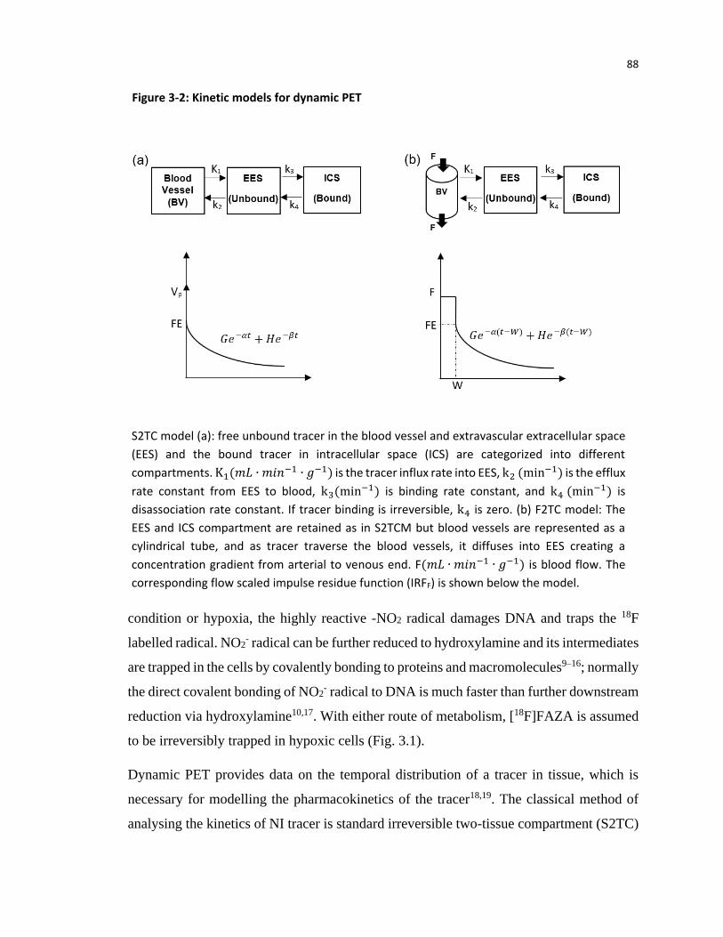
(A) Schematic of standard two tissue compartment model. Besides the blood vessel
compartment, the two tissue compartments are one for free unbound tracer and one for
bound tracer. The extravascular space (compartment) includes both tissue compartments.
Rate constants describing the tracer transfer between compartments are defined in the text.
(B) Corresponding impulse residue function for the model
Figure 1-2: Standard two tissue compartment (S2TC) model
Vp
23
𝑑𝐶𝑒
𝑑𝑡= 𝐾1𝐶𝑝 + 𝑘4𝐶𝑚 − (𝑘2 + 𝑘3)𝐶𝑒 … … … (1)
𝑑𝐶𝑚
𝑑𝑡= 𝑘3𝐶𝑒 − 𝑘4𝐶𝑚 … … … (2)
The rate constants are - K1 is influx rate constant from blood vessel into the free tracer
compartment in tissue, k2 is the efflux rate constant back to the vessel, k3 is binding rate
constant to the target and k4 is the disassociation rate constant from the target. The ‘mass’
concentration of tracer in the tissue, Q(t) including blood vessels and the two tissue
compartments can be expressed as:
𝑄(𝑡) = 𝑉𝑝𝐶𝑝(𝑡) + 𝐶𝑒 + 𝐶𝑚 … . . (3)
where Vp is the tissue blood volume in units of mL per gram of tissue and Cp(t) is the
arterial concentration in units of mMole per mL of blood or the AIF. E is the extraction
efficiency and product of blood flow (F) with E is K1.
Eqs. (1) and (2) can be solved algebraically using Laplace transform and the solution for
Q(t) can be expressed as:
𝑄(𝑡) = 𝐶𝑝(𝑡) ⊗ 𝐼𝑅𝐹𝐹(𝑡) … … … (4)
𝐼𝑅𝐹𝐹(𝑡) = {
0 0 < 𝑡 < 𝑇0
𝑉𝑝𝛿(𝑡) 𝑡 = 𝑇0
𝐺𝑒−𝛼(𝑡−𝑇0) + 𝐻𝑒−𝛽(𝑡−𝑇0) 𝑡 > 𝑇0
… … … (5)
IRFF(t) is the flow scaled impulse residue function. It is the idealized tissue tracer
concentration in response to the tracer being injected as a tight bolus into the vessels
supplying the tissue and ⊗ is the convolution operator, T0 is the delay in tracer arrival at
the tissue relative to that in the vessel where Cp(t) or AIF is measured. This vessel could
be the radial artery with manual blood sampling or a major vessel, like the aorta, with image
derived AIF. The rest of the (model) parameters in Eq (5) are functions of the rate constants
shown in Fig. 1.2:
24
𝛼 =𝑘2 + 𝑘3 + 𝑘4 + √(𝑘2 + 𝑘3 + 𝑘4)2 − 4𝑘2𝑘4
2… … … (6)
𝛽 = 𝑘2 + 𝑘3 + 𝑘4 − √(𝑘2 + 𝑘3 + 𝑘4)2 − 4𝑘2𝑘4
2… … … (7)
𝐺 =𝐾1(𝛼 − 𝑘3 − 𝑘4)
𝛼 − 𝛽… … … (8)
𝐻 =𝐾1(𝑘3 + 𝑘4 − 𝛽)
𝛼 − 𝛽… … … (9)
For ease of explanation (application of principle of conservation of mass), Q(t), Ce(t), Cm(t)
and Cp(t) in Eqs (1-3) are expressed in natural units of mMole per g of tissue or per mL of
blood. However, through calibration with a water phantom filled with uniform activity and
assuming a tissue density of 1.0, all these variables can be expressed in consistent units of
kBq per mL as measured by PET 29.
Due to the compartmental assumption of blood vessels, delivery of the tracer by blood flow
(F) is not ‘explicitly’ modeled, ‘fresh’ tracer from the supplying blood vessels is assumed
to instantaneously mix uniformly with tracer already present and also instantaneously
washout from the blood vessels. This assumed tracer transport in blood vessels leads to
the incorporation of a Dirac delta function of amplitude Vp at t=T0 for the impulse residue
function, IRFF(t) (Fig. 1.2).
1.2.3.2 Flow Modified Two Tissue Compartment (F2TC) Model
To address the shortcomings of assuming blood vessels as a compartment, we developed a
model where all blood vessels are represented as a ‘pipe’ through which the tracer flows
from arterial end to venous end with mean transit time W. To more realistically represent
the delivery and transport of tracer starting at the blood vessels through to the bound
compartment in tissue, we combine the Johnson-Wilson-Lee model (JWLM)30 and the
S2TC model. As in the JWLM, the perfusion delivery of tracer to the blood vessels as well
as the influx and efflux of tracer to and from the free tracer compartment in the tissue
25
during the transit time were explicitly modelled; this approach results in a tracer
concentration gradient in the vessel from the arterial to venous end as opposed to the
instantaneous mixing and washout in S2TC model (Fig. 1.3).
Schematic of flow modified two tissue compartment model. The tissue compartments, as in
the S2TC model, are the free and bound pool. Blood vessels are a pipe with concentration
gradient from the arterial (Ca(t)) to venous (CV(t)) end with mean transit time W.
Corresponding IRF is below the model. During the transit time of the tracer, the concentration
of tracer in the tissue is constant, as indicated by the rectangular function in the IRF. The area
under the rectangular function is the blood volume (Vp).
Figure 1-3: Flow modified two tissue compartment (F2TC) model
26
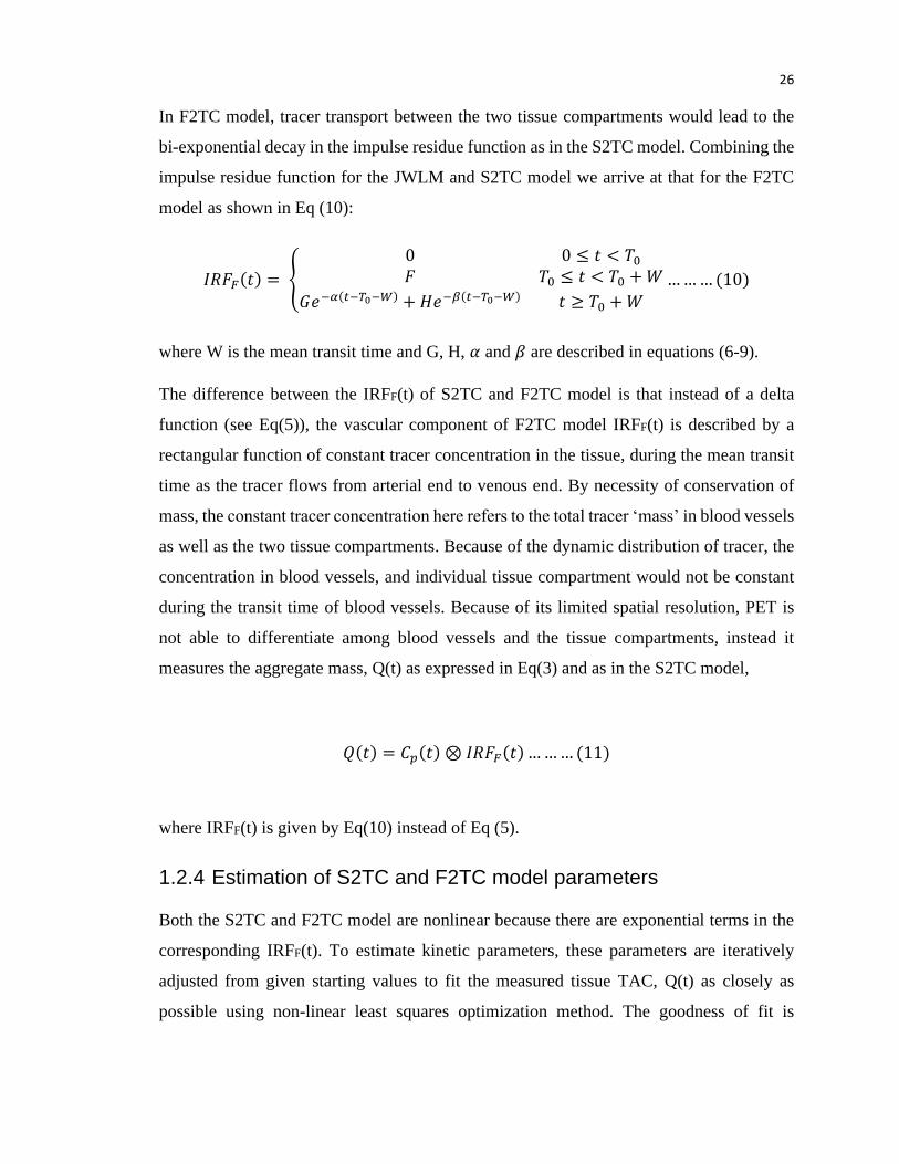
In F2TC model, tracer transport between the two tissue compartments would lead to the
bi-exponential decay in the impulse residue function as in the S2TC model. Combining the
impulse residue function for the JWLM and S2TC model we arrive at that for the F2TC
model as shown in Eq (10):
𝐼𝑅𝐹𝐹(𝑡) = {
0 0 ≤ 𝑡 < 𝑇0
𝐹 𝑇0 ≤ 𝑡 < 𝑇0 + 𝑊
𝐺𝑒−𝛼(𝑡−𝑇0−𝑊) + 𝐻𝑒−𝛽(𝑡−𝑇0−𝑊) 𝑡 ≥ 𝑇0 + 𝑊
… … … (10)
where W is the mean transit time and G, H, 𝛼 and 𝛽 are described in equations (6-9).
The difference between the IRFF(t) of S2TC and F2TC model is that instead of a delta
function (see Eq(5)), the vascular component of F2TC model IRFF(t) is described by a
rectangular function of constant tracer concentration in the tissue, during the mean transit
time as the tracer flows from arterial end to venous end. By necessity of conservation of
mass, the constant tracer concentration here refers to the total tracer ‘mass’ in blood vessels
as well as the two tissue compartments. Because of the dynamic distribution of tracer, the
concentration in blood vessels, and individual tissue compartment would not be constant
during the transit time of blood vessels. Because of its limited spatial resolution, PET is
not able to differentiate among blood vessels and the tissue compartments, instead it
measures the aggregate mass, Q(t) as expressed in Eq(3) and as in the S2TC model,
𝑄(𝑡) = 𝐶𝑝(𝑡) ⊗ 𝐼𝑅𝐹𝐹(𝑡) … … … (11)
where IRFF(t) is given by Eq(10) instead of Eq (5).
1.2.4 Estimation of S2TC and F2TC model parameters
Both the S2TC and F2TC model are nonlinear because there are exponential terms in the
corresponding IRFF(t). To estimate kinetic parameters, these parameters are iteratively
adjusted from given starting values to fit the measured tissue TAC, Q(t) as closely as
possible using non-linear least squares optimization method. The goodness of fit is
27
measured by the root mean squared deviations (RMSD) between the measured and model
fitted curve.
𝑅𝑀𝑆𝐷 = √1
𝑁∑(𝑥𝑖 − 𝑦𝑖)2
𝑁
i= 0
… … … (12)
where xi and yi are the data points of the measured and fitted curve respectively, 𝑖 is the
index of time points and N is the number of time points in the dynamic PET acquisition.
The fitted curve with the least RMSD provides the optimal kinetic parameters for the
measured tissue TAC. For analyzing tracers that are irreversibly bound, the k4 values can
be set to 0. According to central volume theorem31, blood volume, Vp can estimated as:
𝑉𝑝 = 𝐹 × 𝑊 … … … (13)
1.2.5 Graphical Analysis
Graphical Analysis is based on compartmental model but does not require a priori
knowledge of the model structure – number of compartments and their specific
interconnections. It derives summary parameters rather than the rate constants of the model
by linear regression of transformed AIF and tissue TAC. There are two kinds of graphical
analysis: Logan plot is used for analysis of reversibly bound tracer and Patlak for analysis
of irreversibly bound tracer. The major advantage of the method is that it can be used to
validate the reversibility or irreversibility of tracer binding without requiring prior detailed
knowledge of tracer binding mechanism. However, graphical analysis requires the
transformed data to reach linearity which could be affected by noise32.
1.2.5.1 Patlak Graphical Analysis
Patlak plot was initially developed for analysis of influx rate across the blood brain barrier
for irreversibly bound tracer in the brain. The plot is based on non-linear transformation of
the tissue TAC and AIF as shown in the following equation:
28
𝑄(𝑡)
𝐶𝑝(𝑡)= 𝐾𝑖
∫ 𝐶𝑝(𝑡)𝑑𝑡𝑇
0
𝐶𝑝(𝑡)+ (𝑉𝑒 + 𝑉𝑝) … … … (14)
where 𝑄(𝑡) and 𝐶𝑝(𝑡) are the tissue TAC and AIF respectively. The slope of the linear
regression of the transformed data is the unidirectional influx rate constant (Ki) which is
the ratio of the mass of tracer diffused out of vessel to that of the tracer plasma
concentration under equilibrium distribution condition33.
The intercept of the Patlak plot is 𝑉𝑒 + 𝑉𝑝, where Ve is the distribution volume of free and
unbound tracer33–35.
With the S2TC and F2TC model, the unidirectional influx rate constant of tracer can be
expressed in terms of the model rate constants as:
𝐾𝑖 =𝑘1𝑘3
𝑘2 + 𝑘3… … … (15𝑎)
For reversible binding tracer, besides the unidirectional influx rate constant from blood
vessels to the bound compartment, NET influx rate constant is given as:
𝐾𝑛𝑒𝑡 =𝑘1𝑘3
𝑘2 + 𝑘3 + 𝑘4… … … (15𝑏)
1.2.5.2 Logan graphical analysis
Logan plot is used for analyzing tracers that are not irreversibly bound to the target, that is,
k4 is non-zero. The equation describing the plot is:
∫ 𝑄(𝑡)𝑑𝑡𝑡
0
𝑄(𝑡)= VT.
∫ 𝐶𝑝(𝑡)𝑑𝑡𝑇
0
𝑄(𝑡)+ 𝐼𝑛𝑡. … … … (16)
It plots the integral of tissue TAC against integral of arterial TAC, both normalized by Q(t).
The slope of the curve is the total distribution volume (VT). The plot is linear when the
intercept (Int.) becomes constant34.
29
𝐼𝑛𝑡. =𝐶e(t) + 𝐶m(𝑡)
𝐶𝑝(𝑡)… … … (17)
Here VT is a theoretical volume defined as the ratio of tracer concentration in the tissue
(free and bound compartment) to that in blood vessel at distribution equilibrium. Similar
to Patlak plot, VT can also be expressed in terms of rate constants of the S2TC or F2TC
model as:
𝑉𝑇 =𝐾1
𝑘2(1 +
𝑘3
𝑘4) + 𝑉𝑝 … … … (18)
For a one tissue compartment model or for modelling inert tracers, distribution volume
(DV) is equivalent to Ve which is DV for free and unbound tracer (excluding Vp)35 and it
is expressed as:
𝑉𝑒 = 𝐷𝑉 =𝐾1
𝑘2… … … (19)
1.2.6 Spectral Analysis
Like graphical analysis, spectral analysis is also data driven rather than based on a proposed
model. If the distribution of tracer is linear and stationary in time as well as that the PET
signal (image intensity) is linear with respect to tracer concentration, based on the principle
of linear superimposition, the tissue TAC corresponding to an intravenous injection of the
tracer is given by Eq (4). However, instead of two decaying exponentials as in the case of
S2TC model, the IRF(t) is defined by a pre-defined number of exponents (usually 100-
1000):
𝐼𝑅𝐹(𝑡) = ∑ 𝐴𝑖𝑒−𝛼𝑖𝑡
𝑛
i=0
… … … (20)
where 𝑖 is the index of the n predefined exponentials and 𝐴𝑖 is the coefficient of the ith
exponential. The Ai’s can be estimated with linear least square method, preferably with
non-negative constraint27. The advantage of spectral analysis is that it does not presuppose
30
the number of exponentials (compartments and their interconnection), that is, it is
‘agnostic’ to compartment structure. This ‘agnostic’ nature of the spectral analysis would
have the shortcoming that it is difficult to relate exponentials with non-zero Ai’s to rate
constants of specific kinetic processes, for example, influx rate constant of tracer from
blood vessels to tissue or binding rate constant of tracer to its target etc.
1.3 Cancer Imaging
Cancer cells are rapidly growing cells and glucose is the main source of energy for their
metabolism. 18F-FDG is an analog of glucose and like glucose, it is rapidly transported into
cancer cells. Unlike glucose, 18F-FDG does not partake in the subsequent glycolysis steps
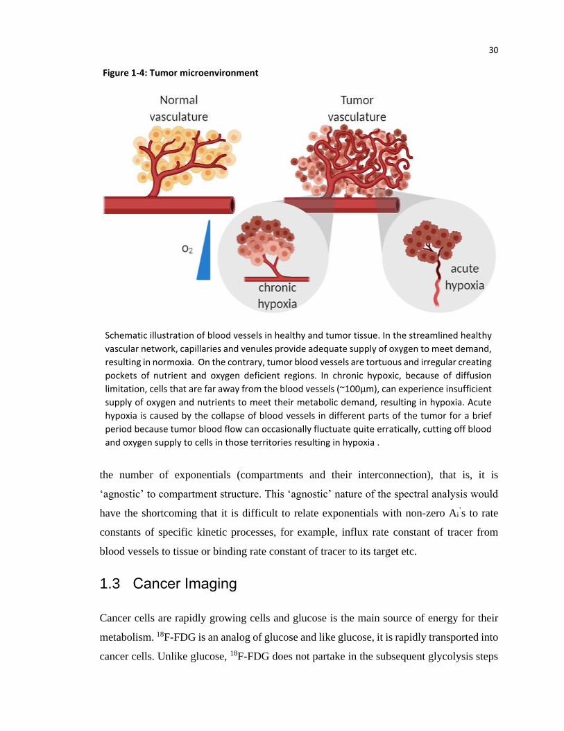
Schematic illustration of blood vessels in healthy and tumor tissue. In the streamlined healthy
vascular network, capillaries and venules provide adequate supply of oxygen to meet demand,
resulting in normoxia. On the contrary, tumor blood vessels are tortuous and irregular creating
pockets of nutrient and oxygen deficient regions. In chronic hypoxic, because of diffusion
limitation, cells that are far away from the blood vessels (~100µm), can experience insufficient
supply of oxygen and nutrients to meet their metabolic demand, resulting in hypoxia. Acute
hypoxia is caused by the collapse of blood vessels in different parts of the tumor for a brief
period because tumor blood flow can occasionally fluctuate quite erratically, cutting off blood
and oxygen supply to cells in those territories resulting in hypoxia .
Figure 1-4: Tumor microenvironment
31
after the initial phosphorylation by hexose due to the labelling of 18F in the C-2 position.
[18F]FDG is trapped in the cells as 18F-FDG-6-P once it is phosphorylated by glycolysis36.
However, in rapidly growing tumors with heterogeneous distribution of blood vessels, the
insufficient supply of oxygen can result in a hypovascular core leading to hypoxia because
of the imbalance between supply and demand for oxygen from glycolysis as well as other
metabolic and cellular processes. Since [18F]FDG participates in the glycolysis pathway, it
cannot be used for imaging the decreased level of oxygen (hypoxia) in solid tumor.
1.3.1 Hypoxia
Hypoxia is a common feature of solid tumors due to imbalance in the supply and utilization
of oxygen in the uncontrolled tumor cell proliferation. Hypoxia can be classified into two
types: chronic and acute hypoxia (Fig 1.4). Chronic hypoxia is caused by diffusion limited
oxygen transport to the tumor cells. Oxygen and nutrient transport in tissues are dominated
by diffusion. Cells that are in close proximity to blood vessels consume the available
oxygen and nutrient while cells further from vessels are oxygen deprived and not capable
of maintaining their regular cell metabolism. The cells will eventually adapt to the lack of
oxygen which will affect their response to treatment or die resulting in necrotic regions6,37–
39. Hypoxia is defined as a partial oxygen (pO2) pressure < 5mm Hg compared to normal
tissues with pO2 > 40mm Hg40,41.
In solid tumors, the vasculature is not streamlined like the normal tissue (Fig. 1.4). The
tortuous structure of the vessels may be perfused only by the plasma or may not be perfused
at all. Despite the presence of vessels, the regional tissues may not be supplied by oxygen.
Hypoxia can also be caused by raised interstitial fluid pressure resulting in intermittent or
cycling hypoxia condition. These perfusion limited and short term hypoxia is called acute
hypoxia which is deemed more resistant to therapy38,42,43.
1.3.2 Hypoxia and radiation resistance
In 1953, Grey et al.41 identified the significance of oxygen in radiation treatment and
hypoxia in treatment resistance. Breathing oxygen before irradiation showed instantaneous
increase in radio-sensitivity with no significant increase beyond pO2 of 20 mmHg. The
32
radio-sensitivity of high linear energy transfer (LET) radiation like neutrons is not
significantly affected with increasing oxygen content. Normal cells can sustain ~3 times
more radiation damage compared to hypoxic cells42,44. With single radiation dose fraction,
hypoxia can limit radio-sensitivity. On the other hand, with fractionated radiotherapy, re-
oxygenation may occur between radiation fractions. This depends on the dose delivered
and on the type of cancer cell45,46.
Radiation kill cells either directly by DNA damage, particularly for high LET radiation like
electrons and neutrons or indirectly via intermediary products like free radicals. The more
common cell death is through the indirect method. It refers to interaction of radiation with
macromolecules in the cytoplasm to liberate high energy electrons which in turn interacts
with other molecules like water. The electrons interaction with water creates highly
reactive hydroxyl radicals which can be removed by recombination with other free radicals
(like �̇� to produce water) or by hydrogen donated from thiol compounds (such as
glutathione, GSH) to produce much less reactive (damaging) radicals. The hydroxyl radical
can combine with oxygen to form highly reactive oxygen species (ROS) like peroxyl
radical. All these free radicals can easily diffuse and cause damage away from the origin
of the first interaction. Indirect damage is most common for low LET radiation. Since 70%
of human body is composed of water, most of the radiation induced injury arises indirectly
from the products of interaction with water as described above38,47. Therefore, radiation
cell kill requires oxygen and low oxygen level inhibits DNA double strand break thereby
enhancing cell survival.6,40,44.
1.3.3 Chemo-resistance in hypoxia
Hypoxic cells in an attempt to survive and propagate in an oxygen limited environment,
are likely to develop a more aggressive tumor phenotype. The gene induced by hypoxia is
regulated by a transcription factor called hypoxia inducible factor (HIF-1). It induces the
expression of genes such as vascular endothelial growth factor (VEGF), glucose
transporter-1 (GLUT-1) and multidrug resistance protein (MDR) which have direct or
indirect resistance to chemotherapy48,49.
33
VEGF is also called vascular permeability factor since it increases vessel permeability and
angiogenesis48,50. Increased vessel permeability can lead to increase interstitial fluid
pressure which would impede the delivery of chemo-drugs by perfusion. GLUT-1 is a
transporter protein that facilitates entry of glucose into tumor cells. Under hypoxic
condition in tumors, overexpression of the protein compensates for the higher energy
demand of tumors since glycolysis can occur in low oxygen environment to maintain the
energy supply of tumors51. This alternate pathway could explain why GLUT-1 indirectly
induce chemo-resistance. The role of MDR is discussed in detail under §1.3.7.
1.3.4 Pancreatic cancer
Pancreatic cancer (PCa) also known as pancreatic ductal adenocarcinoma is a cancer of
ductal epithelium and one of the worst solid cancers because of extremely poor prognosis.
According to American National Cancer Institute cancer statistics from 2009-2015, the
overall 5-year survival rate is 9.3% 52. It is difficult to diagnose PCa early since symptoms
do not appear until it is in an advanced stage or has metastasized. Pancreas is a deeply
situated organs surrounded by other organs at very close proximity, hence it metastasizes
easily and it cannot be palpated by health professional during routine exams53. Only 40%
of patients with localized disease is surgically resectable. It has been established that PCa
have low oxygen tension. The partial oxygen pressure (pO2) of tumor is <5 mmHg and
normal pancreatic tissues has a much higher pO2 >24 mm of Hg54. It is highly resistant to
chemotherapy, radiation therapy and immunotherapy55 and low oxygen tension (hypoxia)
is one of the contributing factors.
1.3.5 Treatment options for pancreatic cancer
Surgical resection alone is not sufficient for pancreatic cancer treatment as invariably
microscopic disease remains in the resection margins. Whipple surgery, a surgical
procedure to remove the head of the pancreas along with lymph node dissection, did not
improve the overall survival56. A randomized trial in 1969 found that patients with
unresectable pancreatic cancer treated with 5-fluorouracil (5-FU) along with radiation
therapy had improved survival of 10 months compared to radiation or chemotherapy
34
alone57,58. According to the European Study Group for Pancreatic Cancer 1 Trial, the five
year survival rate for resected pancreatic cancer was 10 percent for patients receiving
chemoradiotherapy (CR) while the percentage was much higher (21%) for those who
received chemotherapy with 5-FU alone59. Another study comparing CR with
chemotherapy in the American cancer database sponsored by American College of
Surgeons and American Cancer Society, showed that radiation improved overall survival
(OS) by ~3 months on average. However, for node negative patients, radiation proved no
benefit to OS 60. Despite these small improvements in survival, prognosis of PCa is still
very poor.
1.3.6 Chemo-resistance in pancreatic cancer
In pancreatic cancer and in many solid tumors, chemo-resistance is from the failure to
accumulate enough concentration of cytotoxic drugs due to the efflux of these drugs from
tumor cells. Proteins mediating the efflux of drugs belong to the ATP binding cassette
(ABC) transporters. The family of ABC transporter responsible for mediating the drug
resistance is the ABC family B and C (ABCB, ABCC), particularly the multidrug
resistance protein (MDR1) P-glycoprotein (P-pg) and multidrug resistance-associated
protein (MRP) 1-9. MRPs are adenosine triphosphate (ATP) dependent transmembrane
protein responsible for efflux of organic anion as well as toxins in the cancer cells including
cytotoxins and drugs. In particular MRP1, MRP2, MRP3 and MRP6 accounts for transport
of lipophilic compounds conjugated to glutathione, glucoronate and sulfate61,62. MDR1 P-
gp is also a membrane protein that directly efflux toxins out of the cells and it is implicated
in chemo-resistance62,63. While there is an increased expression of MDR1-Pg and MRP1
in pancreatic cancer, there is no correlation with tumor staging or grading. Instead, mRNA
for MRP3 and MRP5 are upregulated in pancreatic cancer and correlated with tumor
grading64–66.
35
1.3.7 Measurement of hypoxia
As discussed in §1.3.1-3, oxygen tension is a determinant of response to cancer therapy,
the ability to measure tumor oxygen tension is of significant importance in treatment
planning.
1.3.7.1 Polarography needle electrode system
Several techniques have been developed in the past to measure tissue oxygen tension. One
such system is the commercially available Eppendorf pO2 probe. It is invasive requiring
insertion of the electrode into the tumor; the technique is limited to easily accessible tumors
like the head and neck tumors, breast cancer and skin lesions42,67. For normal superficial
tissue, pO2 as measured by the Eppendorf probe is 40-60mmHg while hypoxic tissues have
pO2 <10mmHg68. In necrotic tumors where the oxygen content is significantly reduced, the
probe cannot differentiate hypoxia from necrosis.
Non-invasive imaging techniques to measure hypoxia have been developed, including
Magnetic Resonance Imaging (MRI) and Positron Emission Tomography (PET).
1.3.7.2 MRI measurement
MRI is an anatomical and functional imaging technique with good spatial resolution.
Different functional information can be achieved with various MRI sequences. Most of the
MRI images are taken using gradient echo (GRE) sequence generated due to changes in
T2* relaxation time. T2
* is a combination of signal due to spin-spin dephasing as well as
inhomogeneity of the magnetic field. T2* weighted GRE sequence is the most commonly
used blood oxygenation level dependent (BOLD) imaging which is influenced by
susceptibility due to changes in oxygenation in the blood. BOLD takes advantage of the
difference in paramagnetism of the deoxy and oxy- hemoglobin in the blood vessel.
Paramagnetism causes large dephasing of spin-spin lattice which further causes
inhomogeneity of water proton spins in the surrounding tissues, resulting in shortening of
T2* signal69. It measures change in the oxygenation in vasculature rather than the tissue pO2
which is important in determining the radiosensitivity69,70. BOLD signal only showed
36
correlation with temporal change in pO2 with no correlation in its magnitude. The signals
can be confounded by several factors like blood flow, hematocrit concentration and the
interconversion of oxy- and deoxy-hemoglobin43,71,72. For measuring oxygen content in the
tissues, a technique similar to BOLD – tissue oxygenation level dependent (TOLD) MRI
can be used. Unlike BOLD, TOLD relies on T1 relaxation which is caused by the presence
of dissolved oxygen73.
1.3.7.3 PET imaging
A more sensitive method capable of measuring cellular oxygen level is PET. Due to
upregulation of GLUTs in tumor cell membrane74 and as HIF-1𝛼 drives glycolytic
enzymes75, [18F]FDG could be used as surrogate marker for hypoxia. However, studies
have reported conflicting results with some reporting that [18F]FDG is not a good marker
for hypoxia6,76,77. The cause of the discrepancies is because under reduced oxygen, the cells
adapt to the environment and it undergoes anaerobic glycolysis instead of aerobic ATP
production pathway. In addition, HIF-1𝛼 is also expressed in normoxic tissues resulting in
non-specific uptake of [18F]FDG6.
Multiple hypoxia PET tracers have been developed in the past. Since hypoxic cells have
limited blood flow to the tissue, sensitivity of the imaging probe is necessary. The contrast
between the hypoxic region and the normoxia region depends on how much the tracer
enters into the cell, the fraction of the tracer that undergoes reduction in the tissue, the rate
of clearance of the tracer from normoxic tissues and the retention time in the hypoxic
cells78. The commonly used nitroimidazole (NI) based hypoxia PET tracer are 18F-
fluoromisonidazole ([18F] FMISO) and 18F-fluoroazomycin arabinoside ([18F]FAZA). NI
were initially developed as radiosensitizers for hypoxic cells40.
In view of the distance the tracers have to diffuse to the tumor cells which varies with
different tumor types, static image acquisition is not an ideal method to distinguish hypoxia
from normoxic tissues. Kinetic modelling which models the distribution and assess the
reaction rate of tracer accumulation is more applicable in quantifying hypoxia79.
37
1.3.7.4 Mechanism of action for nitroimidazoles
Nitroimidazoles are lipophilic compounds and it enter the cell through passive diffusion.
NI undergoes certain degree of reduction in all the cells but in the absence of adequate
oxygen supply, it undergoes further reduction. The nitro groups can be reduced by enzymes
called nitroreductase, the first step of NI compound breakdown. There are two groups of
nitroreductase, based on their reduction ability due to one or two electron transfer78,80:
1. Type 1 nitroreductase: It is oxygen insensitive enzyme, in the presence or absence
of oxygen, it transfers two electrons from nicotinamide adenine dinucleotide
phosphate (NADP) to its nitro group of the NI compound, producing nitroso and
hydroxylamine intermediates. However, the nitroso group is so reactive and the
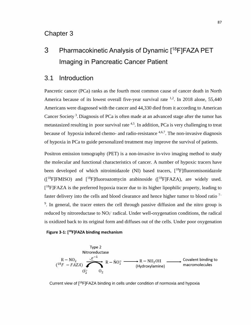
Schematic representation of [18F]FAZA imaging. In normoxia, [18F]FAZA is reduced by type 2 nitroreductase to nitro-oxide radical which in presence of oxygen can revert back to its original form and diffuse out of the cell. Under hypoxia condition, the nitro-oxide radical is converted into nitroso and hydroxylamine that can covalently bind to macromolecule and get trapped in the hypoxic cell.
Figure 1-5: Binding mechanism of [18F]FAZA (nitroimidazole) in hypoxic cell
38
second two-electron transfer to form hydroxylamine is much faster than the first
transfer, it is difficult to isolate the two.
2. Type 2 nitroreductase: It is oxygen sensitive enzyme which catalyzes single
electron reduction to it nitro anion radical. It forms superoxide radical and due to
high oxygen affinity, the radical reverts back to its original form. The cycle
produces oxidative stress by producing large amounts of super-oxides. The
successive steps is determinant in differentiating normal tissue from hypoxic tissue.
In absence of oxygen, the re-oxygenation or formation of superoxide radical is
slowed allowing for further reduction to take place. The superoxide is reduced to
nitroso and hydroxylamine which binds to macromolecules like DNA, RNA and
proteins that eventually gets trapped in the cell81. Due to the oxygen-sensitivity of
this type of nitroreductase, it is of importance in hypoxia imaging.
1.3.8 Hypoxia tracers
[18F]FMISO is a first generation hypoxia NI based tracer. It is a lipophilic tracer which
allows for easy diffusion into the cell. Several studies have shown that the tracer can detect
hypoxia in different tumors types like glioma, head and neck cancer and breast cancer82–84.
Gagel et al. found good correlation between measurements from polarography needle and
[18F]FMISO uptake in head and neck tumor for pO2<10 mmHg after 2 hour of uptake85.
[18F]FMISO have been shown to be a potential tracer to grade gliomas. Using a tumor to
blood radio (T/B) threshold of 1.2, the uptake of tracer was in small in low grade tumor
compared to high grade glioma86. Higher [18F]FMISO uptake was also observed for
estrogen receptor (ER) positive breast cancer and is shown to be a strong predictor of
disease free survival84. Due to the slow plasma clearance of the tracer and hence high
background activity, the tracer needs to be injected for at least two hours before the uptake
of tracer can be visualized. In addition, it requires very low pO2 <10mmHg for significant
[18F]FMISO uptake71,72,81,87.
To address the issue of slow tracer clearance, second generation 2-nitroimidazole was
developed, [18F]fluoroazyomycin arabinoside ([18F]FAZA). The imaging mechanism is
similar to [18F]FMISO. The major advantage of [18F]FAZA is that the tracer is more
39
hydrophilic with higher perfusion and higher clearance and hence higher tumor to
background ratio than [18F]FMISO. Maximal uptake of the tracer is observed at 2 hr p.i.
while there is continual increase in uptake even at 6 hr p.i. for [18F]FMISO87. [18F]FAZA
showed significantly higher uptake of tracer in the hypoxic tumors of pancreatic acinar
tumor cell line compared to [18F]FMISO. Furthermore, the uptake was higher in animal
breathing normal air than in animals breathing pure oxygen88. [18F]FAZA showed
promising result in predicting treatment response for murine breast cancer cell line treated
with chemotherapeutic drug (Triapazamine) along with radiation therapy. Significant
decreased uptake and decreased tumor growth was shown in rats that underwent
chemoradiation while radiation only treatment showed delay in tumor growth89.
1.4 Radio-metabolite production
For detailed analysis of pharmacokinetics of tracer uptake in the diseased tissues, arterial
blood sampling from several time points are required (see §1.2.3). The blood samples or
the imaged derived AIF could be contaminated with metabolites, introducing biases in
kinetic parameter estimation. Upon introduction of tracer into the blood vessel, it is
immediately catabolized by chemicals like enzymes, proteases, oxidizing and hydrolyzing
agent90–92. The biotransformation results in chemically different compounds called
metabolites while the fraction of parent compound decreases. Metabolites that are tagged
with radioactive element are called radio-metabolites. PET detects total signal from
coincidental gamma photons that are emitted due to annihilation event. It is impossible for
the detector to differentiate if the signal is originating from the innate tracer or from the
radioactive element attached to the metabolites. Radio-metabolites are problematic in PET
quantification since metabolites are completely different entity that can have different bio-
distribution93. Therefore, if not accounted for in the blood plasma, can introduce biases in
quantifying any dynamic PET. In addition, if deeper understanding of the physiological
and pathological information is needed, detection and identification of the radio-metabolite
is necessary.
Fractions of unchanged radiotracer in the blood plasma can be measured using high
performance liquid chromatography (HPLC), thin layer chromatography (TLC) and other
40
chromatographic technique. Chromatography techniques are usually limited to the number
of samples that can be analyzed. Blood samples that are taken at later time points suffer
from noisy counting statistics due to reduced tracer activity 94. Different approaches have
been adopted for measuring plasma radio-metabolite. One such method is the
individualized method where fraction of tracer is calculated for each individual patient.
Since each individual patient are limited to small blood sample, it can introduce error due
to sparse sampling. Thus, population-based method where a model is fitted through the
average of the measurement taken across the population is preferred. It removes the
requirement of metabolite measurement for each individual patient, however, the existence
of inter-subject variability can be erroneous.
1.4.1 Separation of radio-metabolites
Several studies in the past have measured radio-metabolites. One such study was done by
Rusjan et al., where he determined blood plasma radio-metabolite for [18F]FEPPA binding
to translocator protein in the brain. The fraction of unmodified tracer was estimated using
reverse phase HPLC. For the tracer, fast metabolism was observed with 80% metabolized
in the first 30 minutes. The rate of metabolism slowed with time with the presence of at
least three radio-metabolites95.
To account for radio-metabolite in the tissue double input compartment model (DICM)
was developed. DICM was used by several studies in the past96–98. Tomasi et al., compared
the kinetic parameters estimated using single input compartment model (SICM), DICM
and double input spectral analysis (DISA) for two tracers: 5-[18F]fluorouracil (5-[18F]FU)
and [18F]fluorothymidine ([18F]FLT). For the tracer 5-[18F]FU, the fit of the curve is
superior with double input method as indicated by Akaike information criteria and the
quality of the fit. Distribution volume between DICM and DISA were in perfect agreement.
Furthermore, the influence of DI method is dependent on the tracer. The method is more
prominent for tracers that have higher metabolism, in this case 5-[18F]FU, compared to 18F-
FLT that has lower rate of metabolism. Radio -metabolite did not show any effect on ki
estimate97.
41
1.4.2 Chromatography
The fraction of unmodified or parent tracer in plasma is measured with chromatography
technique like HPLC, TLC and solid phase extraction (SPE). Chromatography is a
technique used to separate chemical components or analytes in a solvent using two
immiscible liquid called phases, one that is usually fixated to a surface (stationary) while
the mobile one called the mobile phase. The basic principle of chromatographic separation
is that the solvent or the mobile phase containing the sample is continuously transported
through the stationary phase. As the mobile phase flows through the stationary phase, the
interaction between the phases separate or distribute the analytes. The separation is based
on the properties of the phases, as determined by the intermolecular forces like polarity,
ion-ion interaction, and size exclusion and so on. For the thesis in chapter 4, the separation
is based on polarity. Stationary phase in column chromatography is usually a polar solvent
that is fixated into a packing material like silica while in planar chromatography, silica is
a thin monolayer fixated on a solid backing like glass or alumina plate. As the mobile phase
containing the analyte flows through the stationary phase, the difference in the polarity
separates the individual component. The sample flows through the stationary phase at same
velocity as the mobile phase. The analyte that has stronger affinity with the stationary phase
will spend greater proportion of time in the solid phase. In the case of separation based on
polarity, analyte that is the more polar will flow through at a slower rate compared to
analyte that are less polar. The differential spatial retention results in the separation of the
analyte as they move through the system99,100.
The instrumentation of each individual technique is described below:
1.4.2.1 Thin Layer Chromatography (TLC)
Thin layer chromatography is a planar chromatographic technique in which the stationary
phase is supported on a planar surface. For TLC, the stationary phase is a silica gel backed
on a glass or aluminum plate. In planar chromatography, the sample is spotted on a marked
position, usually 1 cm from the bottom of the plate, on the silica surface. The mobile phase
is allowed to develop or evaporate in a development tank with a sealable top. After the
42
development and drying of the spots on the TLC plate, bottom of the plate containing the
spot is immersed in the mobile phase at an upright position such that the mobile phase front
is below the sample spots. As the mobile phase permeates through the silica gel by capillary
action, it separate the analytes based on polarity in the direction of the flow. After the
mobile phase have migrated to specified distance, usually 1cm from the top of the plate,
the plate is removed from the tank and air dried. The point at which the mobile phase
moved furthest is called the solvent front99,101.
TLC is an economical, simple and robust technique. However, it suffers from low spatial
resolution and low sensitivity102. This led to the use of high performance TLC (HPTLC).
It has many improvement compared to TLC in that the particle size of the solid phase in
HPTLC is smaller (5-15µm) compared to 20 µm for conventional TLC. The smaller and
more uniform and thinner layer contributes to reduced background noise, higher efficiency
and tighter spots as a result of reduced spot spreading per plate length. Though HPTLC has
better performance, the price tag associated with the instrumentation have prevented a rapid
growth in its utilization99. Different method involved in detecting the radioactivity for
radioactive sample is discussed in §1.4.3.
Separation of metabolite with TLC based on differences in polarity. Mobile phase acts as the solvent to carry the analyte through the plate by capillary action. In this example, three samples are spotted on the TLC plate and after immersing in the mobile phase for some time, analytes in the samples are separated by their polarity. Since silica is solid phase, the least polar the analyte is, the furthest it will move from the bottom of the plate.
Figure 1-6: Separation of metabolites by Thin Layer Chromatography (TLC)
43
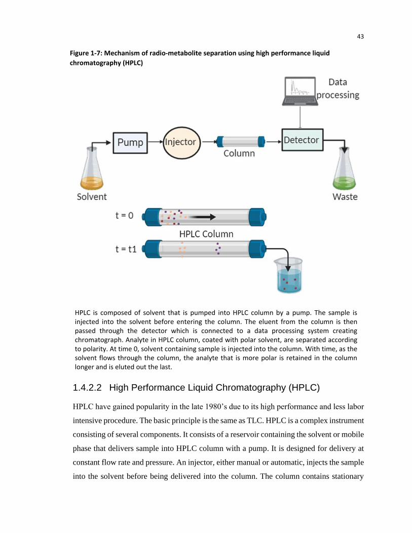
1.4.2.2 High Performance Liquid Chromatography (HPLC)
HPLC have gained popularity in the late 1980’s due to its high performance and less labor
intensive procedure. The basic principle is the same as TLC. HPLC is a complex instrument
consisting of several components. It consists of a reservoir containing the solvent or mobile
phase that delivers sample into HPLC column with a pump. It is designed for delivery at
constant flow rate and pressure. An injector, either manual or automatic, injects the sample
into the solvent before being delivered into the column. The column contains stationary
HPLC is composed of solvent that is pumped into HPLC column by a pump. The sample is injected into the solvent before entering the column. The eluent from the column is then passed through the detector which is connected to a data processing system creating chromatograph. Analyte in HPLC column, coated with polar solvent, are separated according to polarity. At time 0, solvent containing sample is injected into the column. With time, as the solvent flows through the column, the analyte that is more polar is retained in the column longer and is eluted out the last.
Figure 1-7: Mechanism of radio-metabolite separation using high performance liquid
chromatography (HPLC)
44
phase, usually silica packed material, responsible for separating the analyte in the mobile
phase. The eluents containing the analytes are then collected and passed through detectors
for signal generation. Depending on the properties of the mobile phase, the detector system
could be UV light absorbance, conductance, fluorescence or a scintillation detector for
radioactive element (radio-HPLC). The data or signal is then collected by a computer to
generate chromatograph that can be quantified as concentration of analyte in the
solvent99,100,103.
Radio-HPLC is a very sensitive system with high resolution. Both the photons and
positrons can be detected by scintillation detectors. The eluent tube containing the eluents
after analyte separation are coiled for larger surface area. The scintillation detector are
oriented in a way that coincidence photons caused by annihilation photons are detected in
opposite direction thus reducing background noise93,101.
There are pros and cons of using HPLC over TLC. TLC is more economical and robust.
Unlike HPLC where samples are injected serially, TLC can analyze multiple sample at a
time which is especially important for short lived isotopes101. Therefore, for HPLC which
requires an operator to be present can be subjected to unnecessary radiation exposure in
the radioactive samples. HPLC is time limited while TLC is spatially limited. In HPLC
column, the samples flow though same distance and are separated with time influenced by
flow rate of the mobile phase. TLC, on the other hand, all samples have same separation
time and they are separated in space99. The eluting of the column in HPLC with solvent
can clog the column which will require cleaning and unclogging before operation. This
results in ‘memory’ contamination since the column is reusable and unlike TLC, it is a
single use plate. For TLC, there are more robust against minor impurities in the stationary
phase matrix93,101. HPLC boasts of higher spatial resolution compared to TLC.
1.4.2.3 Solid phase extraction (SPE):
Solid phase extraction is a chromatographic technique104 with several advantages over TLC
and HPLC. It requires less solvent, easier to use, convenient and it can easily be automated.
It is based on the principle of separation by filtration and decantation by retaining or
absorbing the analytes from the sample with stationary phase immobilized on a packing
45
material. Silica is usually used as the packing material contained in a cartridge. The general
first step of separation is preconditioning the cartridge for removal of contaminants in order
to improve the efficiency, performance and reproducibility of result. Preconditioning
involves passing a small volume of appropriate solvent through the cartridge. The sample
is then loaded into the cartridge, followed by washing with a solvent to elute unnecessary
interfering matrix while retaining the analytes in the cartridge for further analysis. The
SPE consists of a cartridge packed with silica gel fiber. The cartridge is preconditioned with a
solvent before loading the sample. It is then washed to remove unnecessary or waste
component followed by elution with a solvent to elute out a least polar analyte. Subsequent
elusions are performed with solvents that are more polar than the previous ones to elute out
analytes more polar than the preceding ones. The eluted solvents are then passed through
detector for activity measurement or an HPLC for analyte identification.
Figure 1-8: Separation of metabolites using Solid Phase Extraction (SPE)
46
analyte is eluted out of the cartridge with a stronger solvent either by gravity or vacuum
suction mechanisms. For solvent with more than one analyte, second elution is necessary
but with a stronger solvent 99,104. For extraction based on polarity, the subsequent eluent
will be more polar than the previous ones. In radioactive samples, the activity of the analyte
in the eluents are counted using a 𝛾 counter. For identification of the analytes, the eluents
can be further analyzed by HPLC105.
Since the separation is based on physical separation, real time separation cannot be
observed. Hence, it is not possible to estimate the number of times the cartridge need to be
eluted for extraction of all the metabolites. Another limitation of the technique is the loss
of analyte on the packing material during filtration process99. It is a very fast method and
the cartridges (Waters Corporation) are cheap and unbreakable104. Depending on the
samples analyzed, like HPLC, cartridges with different packing materials are available.
1.4.3 Detection of radioactivity on TLC
TLC contains very minute amount of radioactivity which necessitates the use of a very
sensitive detector or technique for characterization. Some of earlier technique is zonal
analysis that involves the use of liquid scintillation counting (LSC) method. In this
technique, spot on the silica gel or the paper containing the separated analytes are scraped
off, mixed with scintillation fluid and the activity measured using LSC. This technique is
very time consuming and labor intensive and there is huge probability of losing the
analyte106,107. Radio-TLC scanner is less labor intensive where 2D chromatographs can be
acquired. It has low counting and detection efficiency with 1-7 mm of scanning step,
resulting in poor spatial resolution. For determining the small fraction of radio-metabolite
containing trace radioactivity, the technique is not a suitable option. The use of
autoradiography overcomes the limitations. In this system, the TLC plate is placed directly
on X-ray film for counting. Photo-densitometry or scintillation detector converts the counts
into a chromatograph as dark spots or regions of different optical density107. For weak 𝛽-
emitter like 3H, long exposure time of hours or weeks is necessary for good signal
intensity99,106,108. In addition, the lower limit of detection is very high. Though
autoradiography have high resolution it suffers from very poor sensitivity.
47
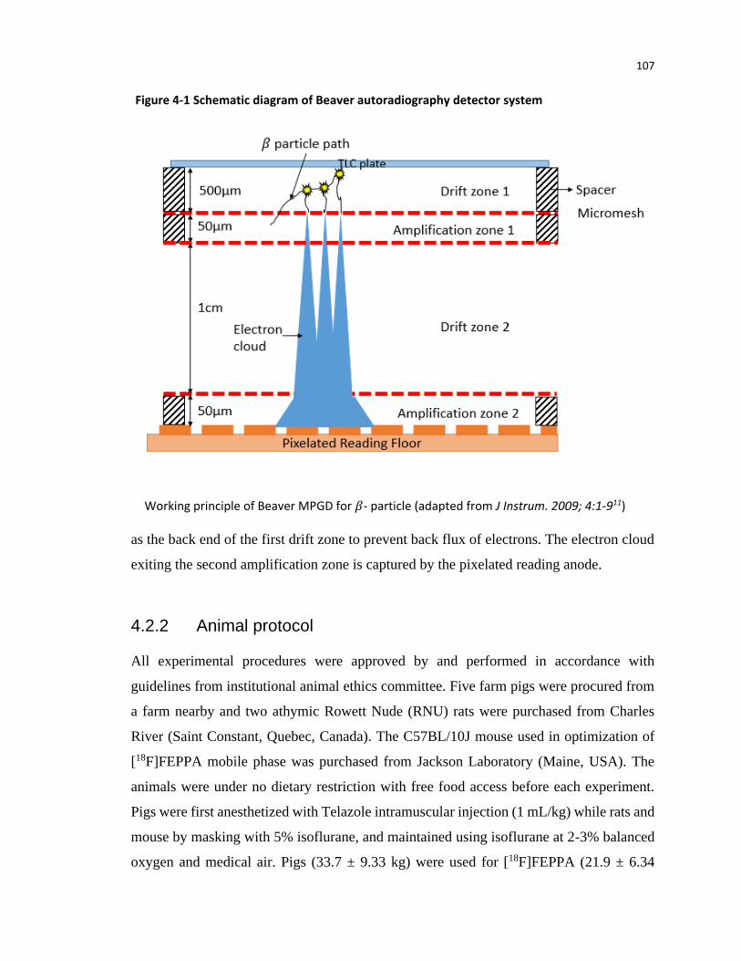
In this work, use of a very sensitive detector is required to detect low radioactivity
contained in 2µL of plasma on the TLC plate. One such system is the Beaver
autoradiography (ai4r, France), mainly used for analyzing tissue and plant samples. It is
used for analyzing beta and alpha particles by detecting electrons produced by ionization
caused by particles emitted from radioactive decay109. The system is based on the principle
of micro pattern gaseous (Ne + CO2) detector (MPGD)110. It consists of two drift zones
alternating with two amplification zone, separated by 5𝜇𝑚 thick nickel micromesh with
varying electric field (Fig. 4.1). The first and third zones are drift zones with low electric
field (1kV/cm) to guide the electrons into the amplification zone. Due to high electric field
of 20-30 kV/cm in the amplification zone, enough kinetic energy is imparted to the
electrons to cause ionization by avalanche effect. Since TLC plate is used as cathode and
it is comprised of highly insulating material, first drift zone is in contact with the plate to
prevent back flux of electrons. The electron clouds exiting the second amplification zone
are captured by the pixelated reading anode. The small thickness of amplification zone
ensures that the avalanche electron clouds are narrow and hence excellent spatial
resolution. The system has very high sensitivity of 5x10⁻⁴ cpm/mm2 and spatial resolution
of 50 µm (for high energy beta and beta plus particle)111 and 30µm as measured by 3H (low
energy beta particle)110.
1.5 Research goal and objectives
The main goal of the thesis is to improve the accuracy of kinetic model’s parameter
estimation and apply them in clinical cancer patient data. The objectives were
accomplished in three stages:
1. The first objective is to develop a generic model for dynamic PET by incorporating
the finite transit time of the tracer from the arterial end to venous end into the
standard compartment model which suffers from non-physiological assumption of
instantaneous arrival and washout of tracer in the blood vessel. The study utilized
simulation to estimate the accuracy of kinetic parameters using the developed
model and the currently used standard compartment model.
48
2. The second objective is to demonstrate that our developed model can be applied to
real clinical patient data that was scanned with dynamic PET. The estimated
parameters were compared with parameters estimated with standard compartment
model and the estimated parameters were utilized in differentiating tumors from
normal tissues. Furthermore, the reversibility of tracer binding was established
using model independent graphical analysis method.
3. The third objective is to correct for radio-metabolite in the blood plasma. Most
tracers introduced in the body will get metabolized into other radioactive products
of different identity that can introduce errors in kinetic parameter estimation.
1.6 Thesis outline
1.6.1 Estimation of kinetic parameters for dynamic PET imaging: A
simulation study
Kinetic parameters estimated by the developed F2TC and S2TC model were compared.
Mean fractional Euclidean distance (FED) averaged all simulated parameter sets was used
as a measure of accuracy. Mean FED is a measure of bias between the estimated and
simulated parameter values. The accuracy is compared across factors that could affect the
parameter estimation - acquisition time, noise level, mean transit time and different models
(F2TC and S2TC). S2TC model is executed with two different software: our custom
MATLAB version and a commercially available software called PMOD. Distribution
volume estimated with the models were also compared with those estimated from graphical
analysis method. The paper will be submitted under the title – Estimation of Kinetic
Parameters for Dynamic PET Imaging: A Simulation Study.
1.6.2 Pharmacokinetic analysis of dynamic [18F]FAZA PET imaging in
pancreatic cancer patient
The kinetics behind the binding of [18F]FAZA in hypoxic pancreatic adenocarcinoma
tumor were investigated with both S2TCM and F2TCM. Model independent graphical
49
analysis model was utilized in estimating the reversibility of tracer binding. The DV from
F2TC model was compared with DV from graphical method. Furthermore, the estimated
kinetic parameters from both F2TCM and S2TCM was utilized in distinguishing the
hypoxic tumor from normoxia tissues. The paper will be submitted under the title –
Pharmacokinetic Analysis of Dynamic [18F]FAZA PET Imaging in Pancreatic Cancer
Patient.
1.6.3 Plasma radio-metabolite analysis of PET tracers for dynamic
PET imaging: TLC and autoradiography
Metabolites in the normal animals’ blood plasma (pig and rat) were separated with thin
layer chromatography (TLC). The low activity of the blood analyte or radio-metabolites
were detected using Beaver autoradiography. The fraction of unmodified tracers were
analyzed for [18F]FEPPA and [18F]FAZA, an inflammatory and hypoxia marker
respectively. Simulation study was done on 10 parameter sets to estimation the error
introduced if radio-metabolite is not corrected in the blood plasma during kinetic analysis
of dynamic PET. The paper will be submitted under the title – Radio-metabolite Analysis
of PET Tracers in Plasma for Dynamic PET Imaging: TLC and Autoradiography
1.7 References:
1. Lee TC, Alessio A, Miyaoka R, Kinahan P. Morphology supporting function: attenuation correction for SPECT/CT, PET/CT, and PET/MR imaging. Q J Nucl Med Mol Imaging. 2016;60(1):25-39. doi:10.1016/j.physbeh.2017.03.040
2. Cherry S, Dahlbom M. PET: Physics, instrumentation, and scanners. In: Phelps M, ed. PET. Springer-Verlag, New York; 2006:1-117. doi:10.1007/0-387-34946-4
3. Raylman RR, Caraher JM, Hutchins GD. Sampling requirements for dynamic cardiac PET studies using image-derived input functions. J Nucl Med. 1993;34(3):440-447.
4. Strother SC, Casey ME, Hoffman EJ. Measuring PET Scanner Sensitivity: Relating Countrates to Image Signal-to-Noise Ratios using Noise Equivalent Counts. IEEE Trans Nucl Sci. 1990;37(2):783-788. doi:10.1109/23.106715
5. Warburg O. The metabolism of carcinoma cells. J Cancer Res. 1925;9(1):148-163. doi:10.1158/jcr.1925.148
50
6. Mees G, Dierckx R, Vangestel C. Molecular imaging of hypoxia with radiolabelled agents. Eur J Nucl Med Mol Imaging. 2009;36:1674-1686. doi:10.1007/s00259-009-1195-9
7. Zhu A, Lee D, Shim H. Metabolic PET imaging in Cancer Detection and Therapy Response. Semin Oncol. 2011;38(1):55-69. doi:10.1053/j.seminoncol.2010.11.012.Metabolic
8. Boellaard R. Standards for PET image acquisition and quantitative data analysis. J Nucl Med. 2009;50:11-20. doi:10.2967/jnumed.108.057182
9. Vanderhoek M, Perlman SB, Jeraj R. Impact of different standardized uptake value measures on PET-based quantification of treatment response. J Nucl Med. 2013;54(8):1188-1194. doi:10.2967/jnumed.112.113332
10. Huang SC. Anatomy of SUV. Nucl Med Biol. 2000;27(7):643-646. doi:10.1016/S0969-8051(00)00155-4
11. Keyes JW. SUV: Standard uptake or silly useless value? J Nucl Med. 1995;36(10):1836-1839.
12. Adams MC, Turkington TG, Wilson JM, Wong TZ. A systematic review of the factors affecting accuracy of SUV measurements. Am J Roentgenol. 2010;195:310-320. doi:10.2214/AJR.10.4923
13. Vriens D, Visser EP, De Geus-Oei LF, Oyen WJG. Methodological considerations in quantification of oncological FDG PET studies. Eur J Nucl Med Mol Imaging. 2010;37(7):1408-1425. doi:10.1007/s00259-009-1306-7
14. Thie JA. Understanding the standardized uptake value, its methods, and implications for usage. J Nucl Med. 2004;45(9):1431-1434.
15. Lammertsma AA. Forward to the past: The case for quantitative PET imaging. J Nucl Med. 2017;58(7):1019-1024. doi:10.2967/jnumed.116.188029
16. Suzuki K, Nishioka T, Homma A, et al. Value of fluorodeoxyglucose positron emission tomography before radiotherapy for head and neck cancer: Does the standardized uptake value predict treatment outcome? Jpn J Radiol. 2009;27(6):237-242. doi:10.1007/s11604-009-0330-7
17. Menda Y, Boles Ponto LL, Dornfeld KJ, et al. Kinetic Analysis of 3’-Deoxy-3’-18F-Fluorothymidine (18F-FLT) in Head and Neck Cancer Patients Before and Early After Initiation of Chemoradiation Therapy. J Nucl Med. 2009;50(7):1028-1035. doi:10.2967/jnumed.108.058495
18. Hamberg LM, Hunter GJ, Alpert NM, Choi NC, Babich JW, Fischman AJ. The dose uptake ratio as an index of glucose metabolism: Useful parameter or oversimplification? J Nucl Med. 1994;35(8):1308-1312.
19. Brendle C, Kupferschläger J, Nikolaou K, La Fougère C, Gatidis S, Pfannenberg C. Is the standard uptake value (SUV) appropriate for quantification in clinical PET imaging? -
51
Variability induced by different SUV measurements and varying reconstruction methods. Eur J Radiol. 2015;84(1):158-162. doi:10.1016/j.ejrad.2014.10.018
20. Fletcher JW, Kinahan PE. PET-CT Standardized Uptake Values (SUVs) in Clinical Practice. Semin Ultrasound CT MR. 2010;31(6):496-505. doi:10.1053/j.sult.2010.10.001.PET/CT
21. Hain SF, Curran KM, Beggs AD, Fogelman I, O’Doherty MJ, Maisey MN. FDG-PET as a “metabolic biopsy” tool in thoracic lesions with indeterminate biopsy. Eur J Nucl Med. 2001;28(9):1336-1340. doi:10.1007/s002590100563
22. Greco C, Nehmeh SA, Schöder H, et al. Evaluation of different methods of 18F-FDG-PET target volume delineation in the radiotherapy of head and neck cancer. Am J Clin Oncol Cancer Clin Trials. 2008;31(5):439-445. doi:10.1097/COC.0b013e318168ef82
23. Willemsen ATM, Hoff J van den. Fundamentals of quantitative PET data analysis. Curr Parmaceutical Des. 2002;8(16):1513-1526.
25. Asselin MC, Cunningham VJ, Amano S, Gunn RN, Nahmias C. Parametrically defined cerebral blood vessels as non-invasive blood input functions for brain PET studies. Phys Med Biol. 2004;49(6):1033-1054. doi:10.1088/0031-9155/49/6/013
26. Watabe H, Channing MA, Riddell C, et al. Noninvasive estimation of the aorta input function for measurement of tumor blood flow with [15O]water. IEEE Trans Med Imaging. 2001;20(3):164-174. doi:10.1109/42.918468
27. Morris ED, Endres CJ, Schmidt KC, Christian BT, Muzic Jr RF, Fisher RE. Kinetic modeling in positron emission tomography. In: Emission Tomography: The Fundamentals of PET and SPECT. Elsevier Inc.; 2004:499-540. http://tauruspet.med.yale.edu/staff/edm42/chapters/kinetic-modeling-chapter-23-wernick-book.pdf.
29. Bailey DL, Jones T, Spinks TJ. A method for measuring the absolute sensitivity of positron emission tomographic scanner. Eur J Nucl Med. 1991;18:374-379.
30. Lawrence KS St., Lee T-Y. An Adiabatic Approximation to the Tissue Homogeneity Model for Water Exchange in the Brain: II. Experimental Validation. J Cereb Blood Flow Metab. 1998;18(12):1378-1385. doi:10.1097/00004647-199812000-00012
31. Meier P, Zierler KL. On the theory of the indicator-diliution method for measurement of blood flow and volume. J Appliced Physiol. 1954;6(12):731-744.
52
32. Gunn RN, Gunn SR, Turkheimer FE, Aston JAD, Cunningham VJ. Positron Emission Tomography Compartmental Models: A Basis Pursuit Strategy for Kinetic Modeling. J Cereb Blood Flow Metab. 2002;22(12):1425-1439. doi:10.1097/01.wcb.0000045042.03034.42
33. Patlak CS, Blasberg RG, Fenstermacher JD. Graphical evaluation of blood-to-brain transfer constants from multiple-time uptake data. J Cereb Blood Flow Metab. 1983;3(1):1-7. doi:10.1038/jcbfm.1983.1
34. Logan J. Graphical analysis of PET data applied to reversible and irreversible tracers. Nucl Med Biol. 2000;27(7):661-670. doi:10.1016/S0969-8051(00)00137-2
35. Innis RB, Cunningham VJ, Delforge J, et al. Consensus nomenclature for in vivo imaging of reversibly binding radioligands. J Cereb Blood Flow Metab. 2007;27(9):1533-1539. doi:10.1038/sj.jcbfm.9600493
36. Endo K, Oriuchi N, Higuchi T, et al. PET and PET/CT using 18F-FDG in the diagnosis and management of cancer patients. Int J Clin Oncol. 2006;11(4):286-296. doi:10.1007/s10147-006-0595-0
37. Hsieh C, Lee C, Liang J, Yu C, Shyu W. Cycling hypoxia increases U87 glioma cell radioresistance via ROS induced higher and long-term H1F-1 signal transduction activity. Oncol Rep. 2010;24:1629-1636.
38. Grimes DR, Warren DR, Warren S. Hypoxia imaging and radiotherapy: Bridging the resolution gap. Br J Radiol. 2017;90(1076). doi:10.1259/bjr.20160939
39. Chan N, Koritzinsky M, Zhao H, et al. Chronic hypoxia decreases synthesis of homologous recombination proteins to offset chemoresistance and radioresistance. Cancer Res. 2008;68(2):605-614. doi:10.1158/0008-5472.CAN-07-5472
40. Brown JM, Wilson WR. Exploiting tumour hypoxia in cancer treatment. Nat Rev Cancer. 2004;4(6):437-447. doi:10.1038/nrc1367
41. Gray L, Conger A, M E, S H, OCA S. The concentration of oxygen dissolved in tissues at the time of irradiaiton as a factor in radiotherapy. Br J Radiol. 1953;26(312):638-648. doi:10.1259/0007-1285-26-312-638
42. Ballinger JR. Imaging hypoxia in tumors. Semin Nucl Med. 2001;31(4):321-329. doi:10.1053/snuc.2001.26191
43. Challapalli A, Carroll L, Aboagye EO. Molecular mechanisms of hypoxia in cancer. Clin Transl Imaging. 2017;5(3):225-253. doi:10.1007/s40336-017-0231-1
44. Vaupel P, Thews O, Hoeckel M. Treatment resistance of solid tumors: Role of hypoxia and anemia. Med Oncol. 2001;18(4):243-259. doi:10.1385/MO:18:4:243
45. Teicher BA. Hypoxia and drug resistance. Cancer Metastasis Rev. 1994;13(2):139-168. doi:10.1007/BF00689633
53
46. Hong B, Kim J, Jeong H, Bok S, Kim Y, Ahn G. Tumor Hypoxia and Reoxygenation : the Yin and Yang for R adiotherapy. Radiat Oncol J. 2016;34(4):239-249.
47. Bushberg JT, Seibert JA, Leidholdt EM, Boone JM. Radiation Biology. In: Mitchell CW, ed. The Essential Physics of Medical Imaging. 2nd ed. Lippincott Williams & Wilkins; 2012:751-836.
48. Shannon AM, Bouchier-Hayes DJ, Condron CM, Toomey D. Tumor hypoxia, chemotherpeutic resistance and hypoxia-related therapies. Cancer Treat Rev. 2003;29:297-307.
49. Doktorova H, Hrabeta J, Khalil MA, Eckschlager T. Hypoxia-induced chemoresistance in cancer cells: The role of not only HIF-1. Biomed Pap. 2015;159(2):166-177. doi:10.5507/bp.2015.025
51. Wang YD, Li SJ, Liao JX. Inhibition of glucose transporter 1 (GLUT1) chemosensitized head and neck cancer cells to cisplatin. Technol Cancer Res Treat. 2013;12(6):525-535. doi:10.7785/tcrt.2012.500343
52. National Cancer Institute (NCI). Cancer Stat Facts: Pancreatic Cancer. NCI website. https://seer.cancer.gov/statfacts/html/pancreas.html. Published 2019. Accessed January 24, 2020.
53. The American Cancer Society medical and editorial content team. Can Pancreatic Cancer be Found Early? American Cancer Society. https://www.cancer.org/cancer/pancreatic-cancer/detection-diagnosis-staging/detection.html#written_by. Published 2019. Accessed January 28, 2020.
54. Koong AC, Mehta VK, Quynh T Le, et al. Pancreatic Tumors Show High Levels of Hypoxia. Int J Radiat Oncol Biol Phys. 2000;48(4):919-922.
55. Daniel SK, Sullivan KM, Labadie KP, Pillarisetty VG. Hypoxia as a barrier to immunotherapy in pancreatic adenocarcinoma. Clin Transl Med. 2019;8(1). doi:10.1186/s40169-019-0226-9
56. Traverso LW. Pancreatic cancer: Surgery alone is not sufficient. Surg Endosc Other Interv Tech. 2006;20(2 SUPPL.):446-449. doi:10.1007/s00464-006-0052-1
57. Moertel C, Childs Jr. D, Reitemeier R, Colby Jr. M, Holbrook M. Combined 5-fluorouracil and Supervoltage Radiation Therapy of Locally Unresectable Gastrointestinal Cancer. Lancet. 1969;294(7626):865-867. doi:10.1016/s0140-6736(69)92326-5
58. Moertel C, S F, Hahn R, et al. Therapy of locally unresectable pancreatic carcinoma: a randomized comparison of high dose (6000 rads) radiation alone, moderate dose radiation (4000 rads + 5-fluorouracil), and high dose radiation + 5-fluorouracil: The Gastrointestinal Tumor Study Group. Cancer. 1981;48(8):1705-1710.
54
59. Neoptolemos JP, Stocken DD, Friess H, et al. A Randomized Trial of Chemoradiotherapy and Chemotherapy after Resection of Pancreatic Cancer. N Engl J Med. 2004;350(12):1200-1210. doi:10.1056/NEJMoa032295
60. Raoof M, Blakely AM, Melstrom LG, et al. Adjuvant chemotherapy versus chemoradiation in high-risk pancreatic adenocarcinoma: A propensity score-matched analysis. Cancer Med. 2019;8(13):5881-5890. doi:10.1002/cam4.2491
61. Shen H, Paul S, Breuninger LM, et al. Cellular and in vitro transport of glutathione conjugates by MRP. Biochemistry. 1996;35(18):5719-5725. doi:10.1021/bi960098n
62. Deng L, Tatebe S, Lin-Lee Y-C, Ishikawa T, Kuo M. MDR and MRP gene families as cellular determinant factors for resistance to clinical anticancer agents. In: Andersson B, Murray D, eds. Clinically Relevant Resistance in Cancer Chemotherapy. Cancer Treatment and Research. Springer, Boston, MA; 2002:49-66.
63. Zhou J, Liu M, Aneja R, Chandra R, Lage H, Joshi HC. Reversal of P-glycoprotein-mediated multidrug resistance in cancer cells by the c-Jun NH2-terminal kinase. Cancer Res. 2006;66(1):445-452. doi:10.1158/0008-5472.CAN-05-1779
64. König J, Hartel M, Nies AT, et al. Expression and localization of human multidrug resistance protein (ABCC) family members in pancreatic carcinoma. Int J Cancer. 2005;115(3):359-367. doi:10.1002/ijc.20831
65. O’Driscoll L, Walsh N, Larkin A, Ballot J, Ooi WS. MDR1 / P-glycoprotein and MRP-1 Drug Efflux Pumps in Pancreatic Carcinoma. Anticancer Res. 2007;27:2115-2120.
66. Chen M, Xue X, Wang F, et al. Expression and promoter methylation analysis of ATP-binding cassette genes in pancreatic cancer. Oncol Rep. 2012;27(1):265-269. doi:10.3892/or.2011.1475
67. Vaupel P, Knoop C, Hockel M. Oxygenationof Human Tumors: Evaluation Of Tissue Oxygen Distribution In Breast Cancers By Computerized O2 Tension Measurements. Cancer Res. 1991;51(12):3316-3322.
68. Xu Z, Li XF, Zou H, Sun X, Shen B. 18F-Fluoromisonidazole in tumor hypoxia imaging. Oncotarget. 2017;8(55):94969-94979. doi:10.18632/oncotarget.21662
69. Fan X, River J, Zamora M, Al-Hallaq H, GS K. Effect of carbogen on tumor oxygenation: combine fluorine-19 and proton MRI measurements. Int J Radiat Oncol Biol Phys. 2002;54(4):1202-1209.
70. Baudelet C, Gallez B. How does blood oxygen level-dependent (BOLD) contrast correlate with oxygen partial pressure (pO2) inside tumors? Magn Reson Med. 2002;48(6):980-986. doi:10.1002/mrm.10318
71. Krohn KA, Link JM, Mason RP. Molecular imaging of hypoxia. J Nucl Med. 2008;49:129S-148S. doi:10.2967/jnumed.110.075663
55
72. Sun X, Niu G, Chan N, Shen B, Chen X. Tumor hypoxia imaging. Mol Imaging Biol. 2011;13(3):399-410. doi:10.1007/s11307-010-0420-z
73. Lyng H, Malinen E. Hypoxia in cervical cancer: from biology to imaging. Clin Transl Imaging. 2017;5(4):373-388. doi:10.1007/s40336-017-0238-7
74. Li S jiao, Guo W, Ren G xin, Huang G, Chen T, Song S li. Expression of Glut-1 in primary and recurrent head and neck squamous cell carcinomas, and compared with 2-[18F]fluoro-2-deoxy-D-glucose accumulation in positron emission tomography. Br J Oral Maxillofac Surg. 2008;46(3):180-186. doi:10.1016/j.bjoms.2007.11.003
75. Semenza GL. Hypoxia, clonal selection, and the role of HIF-1 in tumor progression. Crit Rev Biochem Mol Biol. 2000;35(2):71-103. doi:10.1080/10409230091169186
76. Christian N, Deheneffe S, Bol A, et al. Is 18F-FDG a surrogate tracer to measure tumor hypoxia? Comparison with the hypoxic tracer 14C-EF3 in animal tumor models. 2Radiotherapy Oncol. 2010;97:183-188.
77. Lopci E, Grassi I, Chiti A, et al. PET radiopharmaceuticals for imaging of tumor hypoxia: a review of the evidence. Am J Nucl Med Mol Imaging. 2014;4(4):365-384. doi:10.1038/bjc.2014.610
78. Nunn A, Linder K, Strauss HW. Nitroimidazoles and imaging hypoxia. Eur J Nucl Med. 1995;22(3):265-280. doi:10.1007/BF01081524
79. Shi K, Souvatzoglou M, Astner ST, et al. Quantitative assessment of hypoxia kinetic models by a cross-study of dynamic 18F-FAZA and 15O-H2O in patients with head and neck tumors. J Nucl Med. 2010;51(9):1386-1394. doi:10.2967/jnumed.109.074336
80. Oliveira IM De, Bonatto D, Antonio J, Henriques P. Nitroreductases : Enzymes with Environmental , Biotechnological and Clinical Importance. Curr Res Technol Educ Top Appl Microbiol Microb Biotechnol. 2010:1008-1019.
81. Casciari J, Graham M, Rasey J. A modeling approach for quantifying tumor hypoxia with [F-18]fluoromisonidazole PET time-activity data. Med Phys. 1995;22(7):1127-1139.
82. Bekaert L, Valable S, Lechapt-Zalcman E, et al. [18F]-FMISO PET study of hypoxia in gliomas before surgery: correlation with molecular markers of hypoxia and angiogenesis. Eur J Nucl Med Mol Imaging. 2017;44(8):1383-1392. doi:10.1007/s00259-017-3677-5
83. Bandurska-Luque A, Löck S, Haase R, et al. FMISO-PET-based lymph node hypoxia adds to the prognostic value of tumor only hypoxia in HNSCC patients. Radiother Oncol. 2019;130:97-103. doi:10.1016/j.radonc.2018.09.008
84. Asano A, Ueda S, Kuji I, et al. Intracellular hypoxia measured by 18F-fluoromisonidazole positron emission tomography has prognostic impact in patients with estrogen receptor-positive breast cancer. Breast Cancer Res. 2018;20(1):1-8. doi:10.1186/s13058-018-0970-6
56
85. Gagel B, Reinartz P, DiMartino E, et al. pO2 polarography versus positron emission tomography ([ 18F] fluoromisonidazole, [18F]-2-fluoro-2′- deoxyglucose): An appraisal of radiotherapeutically relevant hypoxia. Strahlentherapie und Onkol. 2004;180(10):616-622. doi:10.1007/s00066-004-1229-y
86. Yamamoto Y, Maeda Y, Kawai N, et al. Hypoxia assessed by 18F-fluoromisonidazole positron emission tomography in newly diagnosed gliomas. Nucl Med Commun. 2012;33(6):621-625. doi:10.1097/MNM.0b013e3283529984
87. Peeters SGJA, Zegers CML, Lieuwes NG, et al. A comparative study of the hypoxia PET tracers [18F]HX4, [18F]FAZA, and [18F]FMISO in a preclinical tumor model. Int J Radiat Oncol Biol Phys. 2015;91(2):351-359. doi:10.1016/j.ijrobp.2014.09.045
88. Piert M, Machulla HJ, Picchio M, et al. Hypoxia-specific tumor imaging with 18F-fluoroazomycin arabinoside. J Nucl Med. 2005;46(1):106-113.
89. Beck R, Röper B, Carlsen JM, et al. Pretreatment 18F-FAZA PET predicts success of hypoxia-directed radiochemotherapy using tirapazamine. J Nucl Med. 2007;48(6):973-980.
90. Pike VW. PET Radiotracers: crossing the blood-brain barrier and surviving metabolism. 2009;30(8):431-440. doi:10.1016/j.tips.2009.05.005.PET
91. Masaki Y, Shimizu Y, Yoshioka T, et al. Imaging mass spectrometry revealed the accumulation characteristics of the 2-nitroimidazole-based agent “pimonidazole” in hypoxia. PLoS One. 2016;11(8):1-11. doi:10.1371/journal.pone.0161639
92. Masaki Y, Shimizu Y, Yoshioka T, et al. FMISO accumulation in tumor is dependent on glutathione conjugation capacity in addition to hypoxic state. Ann Nucl Med. 2017;31(8):596-604. doi:10.1007/s12149-017-1189-9
93. Pawelke B. Metabolite analysis in positron emission tomography studies: Examples from food sciences. Amino Acids. 2005;29(4 SPEC. ISS.):377-388. doi:10.1007/s00726-005-0202-0
94. Veronese M, Gunn RN, Zamuner S, Bertoldo A. A non-linear mixed effect modelling approach for metabolite correction of the arterial input function in PET studies. Neuroimage. 2013;66:611-622. doi:10.1016/j.neuroimage.2012.10.048
95. Rusjan PM, Wilson AA, Bloomfield PM, et al. Quantitation of translocator protein binding in human brain with the novel radioligand 18 F-FEPPA and positron emission tomography. J Cereb Blood Flow Metab. 2011;31(8):1807-1816. doi:10.1038/jcbfm.2011.55
96. Huang S-C, Yu D-C, Barrio JR, et al. Kinetics and modeling of L-6-[18F]fluoro-DOPA in human positron emission tomographic studies. J Cereb Blood Flow Metab. 1991;11(6):898-913. doi:10.1038/jcbfm.1991.155
97. Tomasi G, Kimberley S, Rosso L, Aboagye E, Turkheimer F. Double-input compartmental
57
modeling and spectral analysis for the quantification of positron emission tomography data in oncology. Phys Med Biol. 2012;57(7):1889-1906. doi:10.1088/0031-9155/57/7/1889
98. Mankoff DA, Shields AF, Graham MM, Link JM, Eary JF, Krohn KA. Kinetic analysis of 2-[carbon-11]thymidine PET imaging studies: Compartmental model and mathematical analysis. J Nucl Med. 1998;39(6):1043-1055.
99. Robards K, Haddad PR, Jackson PE. Principles and Practice of Modern Chromatographic Methods. Academic Press; 1994.
100. Scott RP. Mechanism of solute retention in chromatography. In: Brown P r, ed. High Performance Liquid Chromatogrpahy. John Wiley & Sons, Inc.; 1988:117-144.
101. Wilson ID. Thin-layer chromatography: A neglected technique. Ther Drug Monit. 1996;18(4):484-492. doi:10.1097/00007691-199608000-00030
102. Cheng SC, Huang MZ, Shiea J. Thin layer chromatography/mass spectrometry. J Chromatogr A. 2011;1218(19):2700-2711. doi:10.1016/j.chroma.2011.01.077
103. Waters. How does high performance liquid chromatography work? https://www.waters.com/waters/en_US/How-Does-High-Performance-Liquid-Chromatography-Work%3F/nav.htm?locale=en_US&cid=10049055. Accessed January 27, 2020.
104. McDonald PD. A sample preparation primer and guide to solid phase extraction methods development. In: McDonald PD, Bouvier ES., eds. Solid Phase Extraction Applications Guide and Bibliography: A Resource for Sample Preparation Methods Development. 6th ed. Waters Corporation; 1995.
105. Hennion M-C. Solid-phase extraction: method development, sorbents, and coupling with liquid chromatography. J Chromatogr A. 1999;856:3-54.
106. Marx AM, Kronberg H, Neuhoff V. Determination of the specific radioactivity of amino acids by a combination of thin-layer chromatography and quantitative autoradiography. J Chromatogr. 1987;393(19):407-417. doi:10.1017/CBO9781107415324.004
107. Clark T. Radioactivity Detection. In: Encyclopedia of Separation Science. Academic Press; 2000:899-906.
108. Roberts T. Radio-thin layer chromatography. In: Radiochromatography: The Chromatography and Electrophoresis Radiolabelled Compounds. Elsevier Inc.; 1978:45-81.
109. Sardini P, Angileri A, Descostes M, et al. Quantitative autoradiography of alpha particle emission in geo-materials using the BeaverTM system. Nucl Instruments Methods Phys Res Sect A Accel Spectrometers, Detect Assoc Equip. 2016;833:15-22. doi:10.1016/j.nima.2016.07.003
58
110. Donnard J, Arlicot N, Berny R, et al. Advancements of labelled radio-pharmaceutics imaging with the PIM-MPGD. J Instrum. 2009;4(11):1-9. doi:10.1088/1748-0221/4/11/P11022
111. Ai4r. BeaQuant. http://www.ai4r.com/real-time-autoradiography/product/. Published 2017. Accessed January 31, 2020.
59
Chapter 2
2 Estimation of kinetic parameters for dynamic PET
imaging: A simulation study
2.1 Introduction
Positron Emission Tomography (PET) imaging with targeted probes can provide
metabolic, physiologic and molecular information about diseases and their treatment
responses. It also holds great promise for quantitative imaging, in particular kinetics
modelling, however this capability is not fully utilized for different reasons. Currently,
clinical PET is quantified using standardized uptake value (SUV). It is a measure of tracer
uptake in the tissue normalized by the amount of tracer injected and the body weight
derived from an image acquired at a single time point after administration of the targeted
probe. Comparing SUV measured at follow-up to baseline is accepted as a quantitative
measure of treatment response1. While SUV is simple to use and provides reproducible
quantitative assessment rather than subjective visual interpretation of PET images, it is an
imperfect surrogate measure of target concentration/activity. Therefore, the diagnostic
accuracy of SUV is dependent on the properties of the tracer used, for example, fast vs
slow blood clearance, and the particular clinical/research question under investigation2–4.
SUV also varies with the time at which it is measured post administration of the tracer. To
optimize SUV contrast between target and background tissue would require detailed
knowledge of the kinetics of tracer, for example, irreversible vs reversible binding, rate of
binding vs dissociation from target and these rates relative to the bidirectional rates of
tracer permeation of the blood-tissue barrier5,6. These kinetic properties could vary between
patients making optimal SUV measurement for individual patients difficult.
Tissue uptake of targeted tracer is governed by three processes - perfusion delivery,
bidirectional permeation of the blood-tissue barrier during the finite transit time of the
blood vessels, interaction with (i.e. binding to and dissociation from) target. SUV measured
at any time post injection is the balance of these three processes. As each of the uptake
processes requires at least two parameters to describe (see §2.1 below), it is clear a single
60
image (i.e. SUV) is unable to characterize all three processes. This is the motivation for
dynamic PET wherein images at multiple time points post injection are acquired in order
to estimate the three uptake processes. For targeted tracers, the kinetic parameters of
interest include: the rate constants of binding to and dissociation from target as well as the
distribution volume (DV). The rate constants provide a measure of target
concentration/activity and the reversibility of the binding to the target while DV can be
regarded as the theoretical background subtracted SUV when the different processes
involved (as discussed above) in the uptake of the probe are in ‘dynamic’ equilibrium and
is therefore a summary measure of both the bidirectional permeation of the blood-tissue
barrier as well as the binding and dissociation of the targeted probe.
One frequently used method to analyze dynamic PET is kinetic modelling wherein a model
of the tracer uptake processes is used to replicate the tissue uptake vs time or time-activity
curve (TAC) measured by dynamic PET. Compartment models, in particular, the standard
two tissue compartment (S2TC) model with the implicit blood compartment, have been
widely used to analyze dynamic PET studies of targeted tracers. The first tissue
compartment comprises the free (unbound) tracer in the extravascular extracellular space
(EES) from the bidirectional permeation of the blood – tissue barrier while the second
tissue compartment the bound tracer in EES and/or cells. However, modelling blood
vessels as a well-mixed compartment does not accurately describe the delivery and
accumulation of the free tracer in the first tissue compartment, hence would affect the
estimation of the kinetics between the first and second compartment, that is, the binding
and dissociation of the tracer from its target. We have developed the flow modified two
tissue compartment (F2TC) model which models the flow of tracer in blood vessels as well
as the bidirectional permeation of the endothelial barrier between blood vessels and tissue
during the finite transit time through these vessels, in addition to modelling the free and
bound tracer in the tissue as two compartments as in the S2TC model. In this simulation
study, we compared S2TC to F2TC model to investigate the effect of noise, blood vessel
transit time and permeation, and time duration of the dynamic PET study on model
sets and noise was simulated with a Sc of 5. The same fitting software as in §2.4.1 was
used to estimate the model parameters.
2.2.4.3 Effect of MTT on the Estimation of Model Parameters
Since the bidirectional permeation of the endothelial barrier in the F2TC model occurs
during the MTT of blood vessels whereas this process is assumed to happen
instantaneously in the S2TC model, the effect of three different MTTs (5, 10 and 20s) were
observed while other parameters remained the same (as in table 2.1). The MTTs were
chosen to cover larger range of MTTs observed in the hypoxic and ischemic regions. An
acquisition time deemed sufficient from §2.4.2 was used and noise was simulated with Sc
of 5 in this simulation. The same fitting software as in §2.4.1 was used to estimate the
model parameters.
2.2.4.4 Kinetic Parameters Estimation by Different Models/software
As discussed above (§2.2), the compartment assumption for blood vessels in S2TC model
can lead to error in the EES tracer concentration and subsequently error in estimation of 𝐾1
and 𝑘𝑖 , 𝑖 = 2,3,4 and summary parameters like Ki, DV and BP. To test for these modelling
differences, the estimated parameters using F2TC model were compared with those
estimated using S2TC model (with custom software or PMOD) for the 10 parameter sets
in table 2.1 for the case of MTT 20s, Sc 5 and acquisition time of 45 minutes. To remove
the influence of noise but keeping the effect of frame averaging that is ubiquitous in
dynamic PET to improve the signal to noise ratio of tissue TAC, the same comparison
between F2TC and S2TC model was repeated with noise set to zero (Sc =0) while keeping
the other factors the same.
69
2.2.4.5 Numerical Algorithm for the Estimation of Model
Parameters
The noisy curves were fitted with both S2TC and F2TC model using software developed
by ourselves in MATLAB 2019b (The Mathworks Inc.). Besides the in-house custom
software, PMOD (PMOD Technologies LCC.) was also used for fitting with the S2TC
model with blood delay estimation. Fitting with either S2TC or F2TC model is a nonlinear
optimization problem which requires an initial guess of the model parameters as close to
real values as possible to prevent the solution being trapped in local minima. In our in-
house program, the initial guess was estimated using spectral analysis20. In addition, for
robust parameter estimation, sequential search of time delay (T0) and MTT were
implemented. T0 and W (only for F2TC model) were searched from 0 s to 15 s and 0 s to
25 s respectively at 0.5 s intervals. Within the iterative sequential search for T and W, the
rest of the other model parameters – G, H, , and Vp (for S2TC model) or F (for F2TC
model) were estimated with the non-linear optimization routine ‘interior-point’ in
MATLAB. Minimum root mean squared deviation (RMSD) between the fitted curve and
the simulated curve was used as the measure of the best fitted curve. From the fitting
parameters 𝛼, 𝐺, 𝛽 and 𝐻 of the best fitted curve, the explicit model parameters 𝐾1 and
𝑘𝑖 , 𝑖 = 2,3,4 can be calculated using equations (5) and (6).
2.2.4.6 Logan Graphical Analysis for Estimation of Distribution
Volume
The Logan graphical analysis plots the tissue TAC normalized time integral of the tissue
TAC (∫ 𝑄𝑎�̃�(𝑠)𝑑𝑠𝑡
0𝑄𝑎�̃�(𝑡)⁄ ) vs that of the arterial TAC (∫ 𝐶𝑝,𝑎𝑣(𝑠)𝑑𝑠
𝑡
0𝑄𝑎�̃�(𝑡)⁄ ), where
𝐶𝑝,𝑎𝑣(𝑡) is the averaged arterial activity in a dynamic PET image. As discussed by Logan,
after some time the plot becomes linear with a slope equal to the VT7,8,17. The Logan plot is
usually concave (curving upward) before it becomes linear. Therefore, starting from the
origin, the derivative of the Logan plot would increase until it reaches a maximum where
the plot becomes linear. The slope of the Logan plot was determined by linear regression
of data points from the maximum derivative onwards. VT estimated with the Logan plot,
70
F2TC and S2TC (both software) models from TACs of 45 and 60 min duration at a noise
Sc of 5 and MTT of 20 s were compared with the ‘true’ (simulated) value by modified
Bland-Altman analysis21 and non-parametric paired test as in §2.4.4.
2.2.4.7 Analysis of the Simulation Experiment Results
The performance of S2TC and F2TC model and the fitting software was evaluated in each
simulation experiment using fractional Euclidean distance (FED) or root sum of squared
fractional deviations of all explicit parameters from the truth, defined as follows:
𝐹𝐸𝐷 = √(𝑝1 − 𝑝1𝑡𝑟𝑢𝑒
𝑝1𝑡𝑟𝑢𝑒)
2
+ (𝑝2 − 𝑝2𝑡𝑟𝑢𝑒
𝑝2𝑡𝑟𝑢𝑒)
2
+ ⋯ + (𝑝𝑛 − 𝑝𝑛𝑡𝑟𝑢𝑒
𝑝𝑛𝑡𝑟𝑢𝑒)
2
(13)
where 𝑝𝑖, 𝑖 = 1 … 𝑝𝑛 are the explicit F2TC or S2TC model parameters: 𝑛 =
6; 𝑉𝑃, 𝐾1, 𝑘𝑖 𝑖 = 2,3,4, 𝑇0 (W and F parameter in F2TC model were combined and
evaluated as Vp). Results on FED of the estimated parameters were displayed either as the
average and standard deviation (SD) over 50 noisy simulations for each parameter set or,
as average FED and within group SD of all parameter sets. In the pairwise comparison of
estimated FED using different models/software under different conditions described above
(§2.4.1-4), non-parametric paired test (Wilcoxon signed rank test or sign test) on the
median difference of FED between parameter sets was used. Similarly, to test the null
hypothesis that the median difference in the parameters estimated by F2TC and S2TC
71
model (with either custom software or PMOD) was not significantly different from zero.
Non-parametric paired test was used with Bonferroni correction for multiple comparisons.
Either Wilcoxon signed-rank test or sign test was used based on the distribution of the
differences between the groups compared. Unlike Wilcoxon signed test, sign test is not
affected by the symmetrical distribution assumption. All statistical analysis was performed
with SPSS Statistics for Windows, version 26 (SPSS Inc., Chicago, Ill., USA).
Curves used for simulation. (a) Arterial TAC (b) Tissue TAC for parameter set #1 with MTT of 5
s and 20 s. Simulated tissue TAC with (c) noise scaling factor of 1 and MTT of 20 s and (d) with
noise scaling factor of 5 and MTT of 20 s
Figure 2-2: Curves used for simulation experiment
72
2.3 Results
2.3.1 Simulation Curves
Figure 2.2 shows the simulated arterial TAC used in the simulations along with tissue
TACs simulated using the F2TC model. The tissue TACs were generated using parameter
set #1 with two different MTTs: 5 and 20 s. Larger value of MTT results in a wider
rectangular portion in 𝐼𝑅𝐹𝐹. Since tissue TAC is the convolution of arterial TAC with 𝐼𝑅𝐹𝐹,
a longer MTT or vascular transit period would result in a longer time integral of the arterial
TAC and hence a higher tissue TAC.
2.3.2 Comparison between F2TC and S2TC Models at Different
Noise Level
The average FED and the within group SD of the parameter sets are plotted in figure 2.3(a)
and figure 2.3(b) for noise Sc of 1 and 5 respectively. For both noise levels, based on non-
parametric test, median FED for F2TC model was statistically lower than S2TC model with
Comparison of F2TC model and S2TC model with custom software and PMOD at different noise level for simulations with parameter sets from Table 2.1. Average FED and within group SD as error bar at noise Sc of 1 (a) and 5 (b). Data connected by bracket were different with statistical significance indicated by * for P<0.05.
(a) (b)
Figure 2-3: Comparison of F2TC and S2TC model at different noise level
73
either custom software or PMOD (p<0.0015) and median FED for S2TC model was lower
with custom software than PMOD (p< 0.0015). As expected, FED for Sc = 5 is higher than
Sc =1 for all the models/software.
2.3.3 Noise Effect for F2TC and S2TC Models
Figure 2.4 shows the noise effect on the two models and software using average FED for
all parameter sets and the within parameter set SD as error bar. For all models and software,
based on the non-parametric paired comparison (either Wilcoxon signed rank or signed
test, see §2.7), FED was statistically different between all noise levels (p<0.05) with
Bonferroni correction for multiple comparisons (N=3 in this case). Largest average FED
was observed for Sc 5 for both models/software. Though significant, the average FED for
noiseless and Sc 1 were very close to each other with largest average FED difference of
0.04 observed in custom S2TC software.
Average FED and within group SD as error bar for F2TC model, S2TC model with custom software and PMOD (a) at noise Sc of 0 (noiseless), 1, and 5. Data connected by brackets are different with statistical significance indicated by * for P<0.05.
Figure 2-4: Noise effect on F2TC and S2TC model
74
2.3.4 Effect of Dynamic PET Acquisition Time on the Estimation of
Model Parameters
Average FED using different data acquisition times for both models/software are shown in
figure 2.5. Statistical difference in FED was observed for F2TC model when comparing 22
min with 45 (p<0.0015) and 60 min (p < 0.0015) of acquisition. For F2TC with custom
software, the parameter estimation error for 22 min was the highest but the error for 45 and
60 min was comparable suggesting increasing the data acquisition time from 45 to 60
minute might not improve the accuracy of parameter estimation. This was not the case for
the S2TC model with both software, the error did not decrease with longer acquisition time
and no statistical significant difference was found between any time acquisitions for
custom software. Since increasing data acquisition time beyond 45 min did not
significantly affect the parameter estimation for the F2TC model, this time was used for
comparing the effect of MTT and models on parameter estimation.
Average FED with within group SD of all parameter sets as error bar for F2TC model, S2TC model with custom software and PMOD for 22, 45 and 60 min of data acquisition time and noise Sc of 5. Data connected by brackets are different with statistical significance indicated by * for P<0.05.
Figure 2-5: Effect of time acquisition on kinetic models
75
2.3.5 Effect of MTT on the Estimation of Model Parameters
Figure 2.6 shows the effect of MTT on parameter estimation. For the F2TC model, the
error in parameter estimation remained the same as MTT increased from 5 to 10 and 20 s,
despite the error being statistically different between MMT of 10 and 20 s. For S2TC model
with either custom software or PMOD, the error between MTT of 5 and 10s was small even
though for custom software it was significant. The error between MTT of 20 s and 5 or 10
s were all significant with error with MTT of 20 s being the largest.
2.3.6 Estimation of Model Parameters with Different
Models/software
Table 2.2 shows the median differences and limits of agreement (LOA) between the
parameters (both explicit and summary) estimated by F2TC and S2TC (both software)
model for MTT 20 s, Sc 5 and 45 min acquisition. Limits of agreement is defined Q1-
1.5*IQR and Q3+1.5*IQR where Q1 and Q3 are the first and third quartile respectively,
Comparison of error in parameter estimation for 5, 10 and 20 s MTT, with F2TC model and S2TC model with custom software and PMOD, 45 min acquisition time and noise Sc of 5. Data connected by brackets are different with statistical significance indicated by * for P<0.006.
Figure 2-6: Effect of MTTs on model parameters
76
and IQR is interquartile range22. According to non-parametric paired test, the median
difference between parameters estimated by F2TC model and S2TC model with either
custom software or PMOD were significantly different from zero (p<0.004) and the error
was higher for K1, k2 (except PMOD), Vp, DV and BP (all >0.01). Table 2.3 compares the
error for the case of noiseless simulated curves but still with the frame averaging effect.
There is a general trend of the error being larger for all kinetic parameters estimated from
noiseless TAC. Similar to Sc 5 (Table 2.2), larger error was observed for K1, k2, Vp, DV and
BP. PMOD estimated the kinetic parameters with larger error compared to the custom
S2TC model relative to the F2TC model. Table 2.4 compares the parameters estimated by
the F2TC model and custom S2TC model against the simulated (true) parameters showing
larger median differences for custom S2TC model. Tables 2.5 compare the error in
estimated parameters for MTT 10 s, Sc 5 and 45 min acquisition. The median difference
between the parameters estimated by F2TC model and S2TC model (both software) were
significantly different from zero (except BP), LOA being larger for PMOD software. The
LOA for MTT of 10 s shown in table 2.5 was smaller than that for MTT of 20 s in table
2.2.
Table 2.2: Median and limits of agreement (LOA) of difference between the parameters
estimated by F2TC and S2TC model (both software) for MTT 20 s, noise scaling of 5 and 45 min
of acquisition
S2TC (Custom) vs F2TC S2TC (PMOD) vs F2TC
Median Difference LOA Median Difference LOA
K1 -0.010* -0.06 to 0.03 -0.021* -0.13 to 0.07
k2 -0.018* -0.21 to 0.12 -0.006* -0.24 to 0.19
k3 0.006* -0.02 to 0.03 0.009* -0.05 to 0.08
k4 0.002* -0.01 to 0.02 0.002* -0.01 to 0.01
0 VP 0.016* -0.03 to 0.07
0
0.013* -0.04 to 0.08
0 DV -0.013* -0.06 to 0.03 -0.108* -0.33 to 0.08
BP 0.021* -0.32 to 0.30 0.054* -0.51 to 0.72
Ki -0.0005* -0.004 to 0.002 -0.004* -0.02 to 0.01
*Median difference significantly different from zero at P<0.05 with Bonferroni correction for multiple (N=8) comparisons.
77
Table 2.3: Median and limits of agreement (LOA) of difference between the parameters
estimated by F2TC and S2TC model (both software) for MTT 20 s, noise scaling of 0 (noiseless)
and 45 min of acquisition
S2TC (Custom) vs F2TC S2TC (PMOD) vs F2TC
Median
Difference
LOA Median Difference LOA
K1 -0.016* -0.06 to 0.02 -0.037* -0.38 to 0.20
k2 -0.037* -0.14 to 0.05 -0.108* -0.66 to 0.31
k3 0.007 -0.01 to 0.03 0.006 -0.05 to 0.06
k4 0.003* -0.01 to 0.02 0.005 -0.01 to 0.02
VP 0.027* -0.01 to 0.07 0.036* -0.12 to 0.24
DV -0.026* -0.07 to 0.01 -0.115* -0.19 to -0.02
BP 0.050 -0.40 to 0.34 -0.102 -0.89 to 0.66
Ki -0.001 -0.003 to 0.001 -0.005* -0.03 to 0.01
*Median difference significantly different from zero at P<0.05 with Bonferroni correction for multiple (N=8) comparisons.
Table 2.4: Median and limits of agreement (LOA) of difference between the simulated
parameters and parameters estimated by both F2TC and S2TC model (both software) for MTT
20 s, noise scaling of 5 and 45 min of acquisition
F2TC vs Truth S2TC (Custom) vs Truth
Median
Difference
LOA Median Difference LOA
K1 -0.004* -0.07 to 0.06 -0.021* -0.12 to 0.07
k2 0.013 -0.45 to 0.43 -0.047* -0.63 to 0.45
k3 0.024* -0.12 to 0.16 0.024* -0.10 to 0.15
k4 0.003* -0.01 to 0.02 0.006* -0.01 to 0.03
VP 0.012* -0.05 to 0.08 0.033* -0.03 to 0.10
DV -0.016* -0.09 to 0.06 -0.040* -0.12 to 0.04
F -0.222* -1.64 to 0.90 N/A
BP 0.185
.
-1.36 to 1.68 0.139* -1.54 to 1.64
Ki 0.001* -0.01 to 0.02 -0.001* -0.01 to 0.01
*Median difference significantly different from zero at P<0.05 with Bonferroni correction for multiple (N=8) comparisons.
78
Table 2.5: Median and limits of agreement (LOA) of difference between the parameters
estimated by F2TC and S2TC model (both software) for MTT 10 s, noise scaling of 5 and 45 min
of acquisition
S2TC (Custom) vs F2TC S2TC (PMOD) vs F2TC
Median
Difference
LOA Median
Difference
LOA
K1 -0.005* -0.03 to 0.01
-
-0.008* -0.06 to 0.03
k2 -0.009* -0.09 to 0.05 0.003* -0.13 to 0.13
k3 0.003* -0.01 to 0.02 0.006* -0.03 to 0.05
k4 0.001* -0.003 to 0.006 0.001* -0.005 to 0.007
00 VP 0.008* -0.02 to 0.04 0.005* -0.03 to 0.05
DV -0.007* -0.04 to 0.02 -0.059* -0.21 to 0.06
BP 0.017 -0.23 to 0.25 0.060* -0.45 to 0.62
Ki -0.0002* -0.003 to 0.002 -0.001* -0.01 to 0.01
*Median difference significantly different from zero at P<0.05 with Bonferroni correction for multiple (N=8) comparisons.
2.3.7 Logan Graphical Analysis
Figure 2.7 compares estimated VT from the Logan plot, F2TC model and S2TC model with
custom software and PMOD with the true simulated VT value for the cases where MTT was
20 s for all parameter sets of table 2.1 and an acquisition time of either 45 or 60 min. The
estimated VT was compared against the ‘true’ value using a modified Bland-Altman plot
where the x- axis was the average of the estimated VT and the true value while the y-axis
was the difference between the true and estimated VT. Each plot shows 8 instead of 10
cluster lines because two sets of two similar VT’s are clustered together. In each plot, the
solid line is the median difference while the dash are the LOA. For VT estimated by the
F2TC model and Logan analysis, the median difference from the truth became smaller
when the acquisition time increased from 45 to 60 min with the F2TC model being more
accurate than Logan analysis at 60 min (P= 0.2 vs 0.001). The LOA of the F2TC model
also decreased more than Logan analysis as the acquisition time increased. For VT estimated
by the S2TC model with custom software and PMOD and 60 min of data acquisition,
custom software was more accurate than PMOD as well the LOA was larger with PMOD
than custom software.
79
Modified Bland-Altman plot comparing true DV against estimated DV from 45 min (a, b) and 60 minute (c-f) of data acquisition. DV’s were estimated with F2TC model (a, c), Logan analysis (b,d), S2TC model with custom software (e) and with PMOD (f). Details of the plots are described in the text.
Figure 2-7: Comparison of VT estimated by F2TC, S2TC and Logan with simulated VT
80
2.4 Discussion and Conclusion
In this study we demonstrated that the compartmental assumption for blood vessels affects
the accuracy of estimated kinetic parameters because the bidirectional permeation of the
blood-tissue barrier occurs instantaneously rather than over a period, equals to the transit
time of blood vessels. The error was estimated as the average FED over all the parameter
sets where FED is the fractional distance of the estimated from the true set of parameters
in multidimensional parameter space (see equation 13). There was significantly larger error
for both the S2TC model software than F2TC model, with PMOD performing the worst.
As expected, the error was larger for higher noise level for all models/software. Concerning
the length of acquisition time required for accurate parameter estimation, the F2TC model
results show that 45 min was comparable to 60 min in the accuracy of estimated kinetic
parameters and hence is sufficient for parameter estimation from dynamic PET. Due to the
introduction of mean transit time in the F2TC model, we investigated the effect of MTT
from 5 to 10 and 20s. For the F2TC model, FED did not change appreciably with MTT
even though there was significant difference between 10 and 20 s. However, with both the
S2TC software, increasing MTT from 5 to 20 s introduced a 50% increase in FED. In
addition, VT estimated by the F2TC model was more accurate than Logan analysis or the
PMOD software.
Though F2TC model is used for simulating the tissue TAC, errors were observed when the
simulated curve was fitted with the same model. There are several reasons for the errors.
First, estimation of either the S2TC or F2TC model parameters requires the use of non-
linear optimization techniques, which are iterative and depending on the initial estimates
chosen to start the iteration could converge to a local instead of the global minimum,
resulting in errors in the estimated parameters 23. In this study, spectral analysis with the
S2TC model was used to generate the initial parameter estimates that could be ‘close’ to
the global minimum thereby minimizing this source of error. Linearization of tissue TAC
would allow linear least squares methods to be used for model parameter estimation, which
requires much less computation time than iterative non-linear optimization and more
significantly would converge to the global minimum. However, the linearized tissue TAC
involves double integral of the original curve, the correlated noise would lead to biased
81
model parameter estimates 24. Another source of error was frame averaging that is
invariably used in dynamic PET to improve the signal-to-noise of the tissue TAC. In this
study, both the arterial and tissue TAC were simulated at 0.5 s interval, frame averaged
and placed at mid time point of the framing schedule. From table 2.3, it demonstrated that
frame averaging introduced errors in K1 and k2 estimated by the S2TC model (both
software) when compared to the F2TC model.
Figure 2.6 shows that longer mean transit time caused larger average FED of parameters
estimated using the S2TC model with either custom software or PMOD than F2TC model.
In dynamic PET imaging, the tracer is injected intravenously (systematically) and
continues to recirculate throughout the whole body. During each transit of tracer through
the vessels, there is continuous influx and efflux of tracer into the EES (from nonzero K1
and k2 values), failure to properly model the transit time can result in erroneous (larger
bias) K1 and k2 estimate, hence would also affect the downstream k3 and k4. This is
especially important in conditions like ischemic stroke where there is increased mean
transit time with decreased cerebral blood flow and blood volume25. Additionally, S2TC
model’s assumption of instant arrival and washout of tracer led to zero or underestimation
of blood volume which is not physiological and could explain why some kinetic studies
did not report on the estimates of blood volume26–28 or was reported as zero29.
Using FED, figures 2.3-6 showed that the F2TC model is better than the S2TC model with
either the custom software or PMOD. FED being a summary over all parameters is affected
by the parameters related to the vascular effect (K1, k2 and Vp) as well as binding to and
dissociation from target (k3 and k4). Since dynamic PET data are ‘corrupted’ by frame
averaging and noise, a fair comparison of model performance would have to include these
effects. Consistent with these considerations, parameter estimates obtained by the S2TC
and F2TC model on simulated curves that included frame average and noise (see simulation
procedure in §2.4.1) for MTT 20 s were compared. The error in parameters estimated by
the S2TC model with custom software was >0.01 for K1, k2, Vp, DV and BP and <0.01 for
other parameters (table 2.2). With only frame averaging simulation, the error in parameters
estimated by the S2TC model (both software) was higher (table 2.3). With lower MTT of
10 s, the error was reduced to <0.01 for all parameters estimated by the S2TC model with
82
the exception of BP. Taken together, these results support our proposition that ignoring the
transit time effect in blood vessels affect the accuracy in the estimation of vascular
parameters (K1, k2 and Vp) as well as k3 and k4 albeit the effect on the latter two parameters
is less than the first group. Of interest, noise seem to reduce the error of estimated
parameters which could be due to the effect of noise masking the error introduced by frame
averaging. This effect merits further investigation. Another finding is that accuracy of
parameter estimates with PMOD was much poorer compared to the custom software we
developed for the S2TC model. As PMOD is a proprietary software it is difficult to
diagnosis what was the root cause.
Logan analysis is independent of the structure of the compartments and should be more
robust in VT estimation. However, our study showed otherwise − F2TC model estimated
VT was more accurate than Logan analysis. Similar result was also observed by the Logan’s
simulation study where VT estimated by Logan analysis was subject to bias when noise was
present in the tissue TAC 17. The bias increased with VT and noise. The noise dependence
means that it also depends on the physical half-life of the tracer used - shorter half-life
means higher level of noise at later time points of the tissue TAC. Logan analysis plots the
time integral of tissue TAC vs that of the arterial TAC (see § 2.6) and the VT is the slope
of the linear regression line in such a plot. A fundamental assumption of linear regression
is that noise in the data is uncorrelated. However, time integrals add noise of the tissue or
arterial activity at different points together leading to noise correlation. The violation of
the independence of noise would lead to the observed bias in the estimate of VT 24.
In this study, we showed that the F2TC model has better accuracy in estimating kinetic
parameters from dynamic PET imaging than the S2TC model. Noise which is more
prominent in voxel wise than ROI analysis, influences strongly the accuracy and precision
of estimated kinetic parameters. Contrary to current practice, we found that 45 minute of
data acquisition is sufficient for accurate parameter estimation for the 10 sets of parameter
obtained from [18F]FET. Larger parameter sets covering wider range of physiological
conditions will need to be further investigated. One major disadvantage of the F2TC model
is that it is iterative and computationally more expensive due to estimation of W (vessel
mean transit time) and T0 (tracer arrival time) by sequential step-wise search. However,
83
with machine learning or by executing the program in C++, the fitting time can be
29. Dimitrakopoulou-Strauss A, Strauss LG, Schwarzbach M, et al. Dynamic PET
18F-FDG studies in patients with primary and recurrent soft-tissue sarcomas:
Impact on diagnosis and correlation with grading. J Nucl Med. 2001;42(5):713-
720.
87
Chapter 3
3 Pharmacokinetic Analysis of Dynamic [18F]FAZA PET
Imaging in Pancreatic Cancer Patient
3.1 Introduction
Pancretic cancer (PCa) ranks as the fourth most common cause of cancer death in North
America because of its lowest overall five-year survival rate 1,2. In 2018 alone, 55,440
Americans were diagnosed with the cancer and 44,330 died from it according to American
Cancer Society 3. Diagnosis of PCa is often made at an advanced stage after the tumor has
metastasized resulting in poor survival rate 4,5. In addition, PCa is very challenging to treat
because of hypoxia induced chemo- and radio-resistance 4,6,7. The non-invasive diagnosis
of hypoxia in PCa to guide personalized treatment may improve the survival of patients.
Positron emission tomography (PET) is a non-invasive in-vivo imaging method to study
the molecular and functional characteristics of cancer. A number of hypoxic tracers have
been developed of which nitroimidazole (NI) based tracers, [18F]fluoromisonidazole
([18F]FMISO) and [18F]fluoroazomycin arabinoside ([18F]FAZA), are widely used.
[18F]FAZA is the preferred hypoxia tracer due to its higher lipophilic property, leading to
faster delivery into the cells and blood clearance and hence higher tumor to blood ratio 7–
9. In general, the tracer enters the cell through passive diffusion and the nitro group is
reduced by nitroreductase to NO2- radical. Under well-oxygenation conditions, the radical
is oxidized back to its original form and diffuses out of the cells. Under poor oxygenation
Current view of [18F]FAZA binding in cells under condition of normoxia and hypoxia
Figure 3-1: [18F]FAZA binding mechanism
88
condition or hypoxia, the highly reactive -NO2 radical damages DNA and traps the 18F
labelled radical. NO2- radical can be further reduced to hydroxylamine and its intermediates
are trapped in the cells by covalently bonding to proteins and macromolecules9–16; normally
the direct covalent bonding of NO2- radical to DNA is much faster than further downstream
reduction via hydroxylamine10,17. With either route of metabolism, [18F]FAZA is assumed
to be irreversibly trapped in hypoxic cells (Fig. 3.1).
Dynamic PET provides data on the temporal distribution of a tracer in tissue, which is
necessary for modelling the pharmacokinetics of the tracer18,19. The classical method of
analysing the kinetics of NI tracer is standard irreversible two-tissue compartment (S2TC)
S2TC model (a): free unbound tracer in the blood vessel and extravascular extracellular space
(EES) and the bound tracer in intracellular space (ICS) are categorized into different
compartments. K1(𝑚𝐿 ∙ 𝑚𝑖𝑛−1 ∙ 𝑔−1) is the tracer influx rate into EES, k2 (min−1) is the efflux
rate constant from EES to blood, k3(min−1) is binding rate constant, and k4 (min−1) is
disassociation rate constant. If tracer binding is irreversible, k4 is zero. (b) F2TC model: The
EES and ICS compartment are retained as in S2TCM but blood vessels are represented as a
cylindrical tube, and as tracer traverse the blood vessels, it diffuses into EES creating a
concentration gradient from arterial to venous end. F(𝑚𝐿 ∙ 𝑚𝑖𝑛−1 ∙ 𝑔−1) is blood flow. The
corresponding flow scaled impulse residue function (IRFF) is shown below the model.
Figure 3-2: Kinetic models for dynamic PET
89
model (Fig. 3.2a). One limitation of S2TC model is that it does not model the transit of the
tracer through blood vessels rather it is lumped together as the product of the tracer
concentration in (arterial) blood and the blood volume. A consequence is that the estimated
blood volume can be very small particularly if the dynamic PET study has rapid framing
rate (5-10 s per frame) in the first phase and the S2TC model fit includes this fast first
phase. To better describe the transport of tracer into tissue, we combine the Johnson-
Wilson-Lee (JWL) model 20 with the S2TC model to arrive at the flow modified two-tissue
compartment (F2TC) model. It models the flow of tracer in blood vessels and the
bidirectional permeation of the blood-tissue barrier during the finite transit time through
these vessels leading to a concentration gradient from the arterial end to the venous end
(Fig. 3.2b). In contrast, S2TC model assumes the bidirectional permeation of the blood-
tissue barrier occurs ‘instantaneously’ rather than over a period equals to the transit time
of blood vessels.
Contrary to the common understanding of the in-vivo behaviour of NI tracers, some studies
have shown that the tissue time-activity curve (TAC) is best fitted using a reversible S2TC
model21,22. In this study, we investigated the nature of [18F]FAZA binding to pancreatic
tumor in patients using graphical analysis23 and S2TC and F2TC model. As noted above
F2TC model does while S2TC model does not account for the fact that transport of tracer
into tissue occurs over the transit time of the blood vessels rather than instantaneously, use
of both models will show how this effect affects the estimated model parameters. To
confirm model fitting, depending on the nature of tracer binding, forward transfer rate
(plasma to tissue influx rate) for irreversible bound tracer24 or distribution volume for
reversible tracer23 as calculated from the estimated S2TC and F2TC model parameters will
be compared with that estimated by graphical analysis. Finally the estimated model
parameters can shed light on the possible pharmacokinetics and hence the mechanisms
behind the accumulation of [18F]FAZA and washout from tumor cells.
90
3.2 Methods
3.2.1 Patient population and image acquisition
The patient cohort consisted of 20 patients with biopsy confirmed and previously untreated
pancreatic ductal adenocarcinoma. The study was approved by University Health Network
Research Ethics Board and a signed consent form from each enrolled patient was obtained.
Details of the patient population and image acquisition were described previously25,26.
Dynamic images were acquired over 55 min with the following imaging protocol: 12@10s
intervals, 8@30s, 7@120s and 7@300s. PET scans were acquired with in-line PET/CT
scanner (Discovery ST-16; GE Healthcare). Whole tumor TAC was derived from regions
manually contoured by an experienced radiologist in all tumor containing tumor slices.
Arterial input function (AIF) was obtained from aorta at the same level as the tumor ROIs
with no metabolite correction. Out of the 20 patients, only 14 patients had TAC from
normal tissue due to pancreatic atrophy in the remaining patients.
3.2.2 Dynamic PET analysis
Whole tumor TAC and AIF from each patient were analyzed in three ways: graphical
analysis and kinetic analyses using the S2TC and F2TC models.
3.2.2.1 Graphical analysis
It is a compartmental analysis technique which is independent of the number and
connectivity of the compartments and can be used to investigate the nature of the binding
of [18F]FAZA to tumor. For irreversible binding, when tissue TAC (𝑅𝑂𝐼(𝑡)) and AIF
(𝐶𝑝(𝑡)) are transformed as shown in Eq (1), a linear Patlak23,24 plot is obtained following a
short delay where the slope (𝐾𝑖) is the forward transfer rate of tracer from blood to the
bound pool and the intercept is the blood volume (𝑉𝑏):
∫ 𝐶𝑝(𝜏)
𝑡
0𝑑𝜏
𝐶𝑝(𝑡)= 𝐾𝑖
𝑅𝑂𝐼(𝑡)
𝐶𝑝(𝑡)+ 𝑉𝑃 (1)
On the other hand, Eq (2) shows that for reversible binding, the transformed 𝑅𝑂𝐼(𝑡) and
𝐶𝑝(𝑡) after a short delay are linearly related (Logan plot23,27) with slope equal to the sum
91
of the extravascular distribution volume (𝐷𝑉) and blood volume (𝑉𝑃) or total distribution
volume (𝑉𝑇 = 𝑉𝑃 + 𝑉𝐷):
∫ 𝐶𝑝(𝜏)𝑑𝜏
𝑡
0
𝑅𝑂𝐼(𝑡)= (𝑉𝑃 + 𝐷𝑉)
∫ 𝑅𝑂𝐼(𝜏)𝑑𝜏𝑡
0
𝑅𝑂𝐼(𝑡)+ 𝐼𝑛𝑡. (2)
If the plot according to either Eq(1) or Eq(2) is linear, then the tracer is irreversibly or
reversibly bound respectively.
3.2.2.2 Standard two-tissue compartment model (S2TC)
In dynamic PET, the measured tissue activity arises from tracer in the blood vessels, free
unbound tracer in extravascular space and tracer bound in the target. S2TC model
categorizes these different anatomical/physiological states of the tracer as compartments.
In this model, the consequence of modeling blood vessels as a compartment is that tracer
once arrived is assumed to be immediately mixed uniformly with tracer already in the
vessels and to immediately diffuse out to tissue. This is reflected in the flow scaled impulse
residue function (IRFF(t)) where the vascular component is a delta function of area equal
to the blood volume, 𝑉𝑃(𝑚𝑙 ∙ 𝑔−1). IRFF(t) is an idealized tissue TAC if the total amount
of tracer is injected as a tight bolus into a blood vessel supplying the tissue of interest. The
tissue TAC, ROI(t) corresponding to a systemic injection of tracer as in dynamic PET is
obtained by convolution of the AIF with IRFF(t) based on the principle of linear
superimposition. The above discussion is summarized by the following equations:
𝑅𝑂𝐼(𝑡) = 𝐶𝑝(𝑡) ⊗ 𝐼𝑅𝐹𝐹(𝑡 − 𝑇0) (3)
where 𝑇0 is the delay (s) in arrival of tracers from the site where AIF is measured to the
tissue region of interest
𝐼𝑅𝐹𝐹(𝑡) = {𝑉𝑃𝛿(𝑡) 𝑡 = 0
𝐺𝑒−𝛼𝑡 + 𝐻𝑒−𝛽𝑡 𝑡 > 0 (4)
𝛼 =𝑘2 + 𝑘3 + 𝑘4 + √(𝑘2 + 𝑘3 + 𝑘4)2 − 4𝑘2𝑘4
2 (5)
𝛽 =𝑘2 + 𝑘3 + 𝑘4 − √(𝑘2 + 𝑘3 + 𝑘4)2 − 4𝑘2𝑘4
2 (6)
92
𝐺 =𝐾1(𝛼 − 𝑘3 − 𝑘4)
𝛼 − 𝛽; 𝐻 =
𝐾1(𝑘3 + 𝑘4 − 𝛽)
𝛼 − 𝛽 (7)
𝛼, 𝛽, 𝐺 𝑎𝑛𝑑 𝐻 are fitting parameters estimated from curve fitting and it is expressed in
terms of the explicit model parameters K1, k2, k3 and k4 as defined in the legend of Fig. 3.2;
and ⊗ is the convolution operator.
3.2.2.3 Flow modified two-tissue compartment (F2TC) model
To avoid the compartmental assumption for tracer in blood vessels with shortcomings as
discussed above, we developed a new model called flow modified two – tissue
compartment model (F2TC). It models the bidirectional tracer permeation of the blood-
tissue barrier during the finite transit time through blood vessels (Fig. 3.2b). This is
reflected in the IRFF(t) where the delta function in the case of S2TC model is replaced by
a rectangular function with a width equal to the transit time (w) of the tracer from arterial
to venous end of blood vessels. The rest of IRFF(t) remains the same as the S2TC model.
The mathematical representation for F2TC model’s IRFF(t) is:
𝐼𝑅𝐹𝐹(𝑡) = {𝐹 0 ≤ 𝑡 < 𝑤
𝐺𝑒−𝛼(𝑡−𝑤) + 𝐻𝑒−𝛽(𝑡−𝑤) 𝑡 ≥ 𝑤 (8)
The fitting parameters are the same as the S2TC model except that 𝑉𝑃 is replaced by 𝑤 and
can be calculated as the product of 𝑤 and 𝐹 according to the Central Volume Principle 28.
3.2.2.4 Analysis of Tumor and Tissue TAC
PKIN (PMOD technologies LLC, Zurich, Switzerland) with blood delay option was used
to fit the S2TC model to the tumor and normal tissue TAC while custom software
developed in MATLAB (The Mathworks Inc.) incorporating the ‘interior-point’ non-linear
optimization routine was used to fit F2TC model to the same the TACs. The model that
better represented the TACs was determined by comparing the root mean square deviations
(RMSD) between the TAC and the model fit with Wilcoxon signed-rank test and by the
Akaike Information Criteria (AIC 22) for small sample size
93
𝐴𝐼𝐶 = 𝑁. ln (𝑅𝑀𝑆𝐷
𝑁) +
2(𝐾 + 1)(𝐾 + 2)
𝑁 − 𝐾 − 2 (9)
where N is the number of time frames, K is number of parameters in each model. With
explicit model parameters estimated from curve fitting, important summary parameters like
𝐾𝑖 =𝑘1𝑘3
𝑘2+𝑘3+𝑘4 𝑉𝐷 =
𝑘1
𝑘2(1 +
𝑘3
𝑘4) and 𝐵𝑃 =
𝑘3
𝑘4 can be calculated. 𝐾𝑖 is the net influx rate
from the blood vessel to the bound pool and BP the binding potential 29,30. Bland-Altman
plot 31 of median and interquartile extremes of VT estimated with the F2TC and S2TC
model were compared against those estimated by Logan plot. The extremes are calculated
as Q1-1.5*IQR and Q3+1.5*IQR, where Q1 and Q3 are the first and third quartile and IQR
is the interquartile range. Both the summary and explicit parameters estimated by F2TC
and S2TC model were compared using non-parametric paired test. Depending on whether
the distribution of the differences between the two sets of parameters is symmetrical or
asymmetrical, either Wilcoxon signed rank test or sign test, respectively, was used to test
for significant difference between the two models. Univariable logistic regression of
explicit model parameters (VP, K1, ki i=2,3,4) and DV was used to determine their
significance in differentiating normal tissue from cancer. Logistic regression with
backward elimination of a group of above parameters, each selected if the associated
94
univariable analysis attained a P-value of < 0.1, was used to determine the optimal set of
parameters to differentiate normal from hypoxic tumors.
3.3 Results
3.3.1 Reversibility of [18F]FAZA Binding
The non-linear Patlak analysis plot vs the linear Logan analysis plot (Fig. 3.3) proved that
the tracer was reversibly bound contrary to the commonly held view that it is irreversibly
bound. This result was further corroborated by pharmacokinetic analysis where the median
RMSD difference between the model fit and measure TAC in either normal tissue or tumor
was smaller with reversible F2TC model (both and estimated) than the irreversible
model ( set to zero) (z = 3.78, p<0.005).
Linear plot of Logan analysis (a) and non-linear plot of Patlak analysis (b) indicated that the
tracer was reversibly bound contrary to the current view of irreversible binding
Figure 3-3: Graphical analysis of [18F]FAZA tissue TAC from a pancreatic tumor
95
3.3.2 Model selection
As indicated by AIC and RMSD in Fig. 3.4, our developed F2TC model was able to fit the
tumor and normal tissue TAC better than S2TC model (p = 0.002, p<0.0005 respectively).
S2TC model also estimated the blood volume (𝑉𝑃) poorly. The average tumor 𝑉𝑃 estimated
by F2TC and S2TC models, though not significantly different, was 0.1039 and 0.0737 𝑚𝐿 ∙
𝑔−1 respectively with a few S2TC model’s 𝑉𝑃 estimated to be zero which is non-
physiological. According to non-parametric test, the explicit model parameters (Vp, K1, ki
(i = 2,3,4)) as well as the summary parameter BP and Ki estimated by the F2TC and S2TC
model were not significantly different (p> 0.05). However, DV and K1/k2 were
significantly different (p<0.0005). Fig. 3.5 are Bland-Altman plots comparing VT estimated
by Logan analysis against the F2TC and S2TC model. The median differences (thick black
line) and extremes of agreement (dash lines) were significantly lower for F2TC model
compared to S2TC model and VT from F2TC model was not but S2TC model was
significantly different from that estimated by Logan analysis. Extremes of agreement were
Q1-1.5*IQR and Q3+1.5*IQR where Q1, Q3 and IQR are 1st and 3rd quartile and
interquartile range respectively.
Comparison of F2TC and S2TC model in fitting tumor and normal tissue TAC using (a) RMSD and
(b) AIC as measure of goodness of fit. The x-axis is patient number. Case #1-20 corresponds to
tumors and Case #21-34 are normal pancreatic tissues from same patients as 1-20. Normal
tissues were observable in PET imaging in 14 patients only
Figure 3-4: RMS and AIC comparison from F2TC and S2TC model fitting
96
3.3.3 Differentiation of Tumor from Normal Tissue
Among the kinetic parameters estimated with the F2TC model, only k4 and DV were
significant (p<0.05) in univariable logistic regression analysis to separate normal tissue
from tumor. Using a subset of kinetic parameters (Vp, DV and k4), each of which had p<0.1
in univariable analysis, logistic regression with backward elimination identified k4 and DV
as a significant model (p=0.003) to separate normal tissues from hypoxic cancerous tissues
(Fig. 3.6a). The model correctly classified 79% of the cases with specificity of 57% and
sensitivity of 95%. The positive predictive value (PPV) was 76% and negative predictive
value (NPV) 89%. With the S2TC model, univariate analysis showed that only DV had
p<0.1 that correctly classified 71% of cases with sensitivity, specificity, PPV and NPV of
90 %, 43%, 68% and 64% respectively (p = 0.047).
3.4 Discussion
The developed F2TC model models the bidirectional permeation of the blood-tissue barrier
as the tracer traverses the blood vessels over a period equals to the mean transit time,
Bland-Altman plot comparing total distribution volume (VT) estimated for hypoxic and normal tissue with Logan graphical analysis and with (a) F2TC and (b) S2TC model. The solid lines are the median differences and dashed lines are explained in the text.
Figure 3-5: Bland- Altman plots comparing total distribution volume
97
resulting in a concentration gradient from the arterial to venous end of vessels. On the other
hand, S2TC model assumes that fresh tracer in arterial blood is instantaneously and
uniformly mixed with tracer already in the blood vessels and instantaneously washout of
blood vessels. This unrealistic assumption resulted in a smaller VP estimate than the F2TC
model and in some cases even a non-physiological estimate of zero. Total distribution
volume, VT, estimated by the F2TC model for both tumor and normal pancreatic tissue was
not but that estimated by the S2TC model was significantly different from Logan graphical
analysis. This result was also supported by both AIC and RMSD of the fit to the tissue
Distinguishing pancreatic tumor from normal tissue using kinetic parameters estimated with
F2TC and S2TC model. (a) For the F2TC model, distribution volume (DV) and k4 can distinguish
the two tissue types with sensitivity of 95% and (b) For the S2TC model, DV achieved a
sensitivity of 90%. The solid line in each case is the linear discriminator derived from the Youden
index (Cancer 1950; 3(1): 32-35). For each case, DV for one patient’s hypoxic tumor is large
due to zero 𝛽 estimate which was not plotted here but was included in the performance metric
calculations
Figure 3-6: Differentiation of hypoxic tumor from normal tissue with kinetic parameters
estimated by F2TC and S2TC model
98
TAC that the F2TC model was more suited than S2TCM for describing the kinetics of
[18F]FAZA in hypoxic tumor and normal tissue of the pancreas.
The hypoxic pancreatic cancer tissue can be characterized from the normal tissues using k4
and DV from the F2TC model with high sensitivity of 95% and negative predictive value
of 89%. On the contrary, DV from the S2TC model can distinguish the two tissue types
with lower sensitivity and NPV. DV is a surrogate marker of SUV acquired at sufficiently
long time after tracer injection, when the blood background is negligible32. Therefore, using
DV from S2TC model corroborates the usage of SUV for hypoxia imaging in the clinics,
which is performed at least one hour after injection. Nevertheless kinetic analysis by
providing k4 and DV could out-perform SUV (DV) in this diagnostic task.
Mechanisms for hypoxia imaging with nitroimidazole based tracers like [18F]FAZA. The region
indicated by dashed box is the proposed mechanisms behind the reversibility of tracer binding
Cell
Figure 3-7: Proposed binding mechanisms of [18F]FAZA binding
99
Graphical method as well as lower RMSD from the reversible (non-zero 𝛽) F2TC model
compared to the irreversible model demonstrated that the tracer [18F]FAZA was reversibly
bound to hypoxic PCa, contrary to the current view that NI based tracers are trapped in
hypoxic cells. Unlike kinetic modelling, graphical method is independent on the structure
(connectivity) and the number of compartments in the model which makes it more
adaptable to prevailing tumor heterogeneity, i.e. a single F2TC or S2TC model may not
apply to all regions in a tumor. Hence, graphical analysis is a reliable method to determine
the reversibility of tracer binding. Previous studies also corroborated our finding that the
kinetics of NI based tracers are best analyzed using reversible S2TC model21,22.
Nonetheless, the mechanism behind the reversible binding of NI based tracers was not well
described in the literature.
A group in Japan studied the mechanism of NI based [18F]FMISO binding in nude mice by
implanting cells from the human FaDu cancer line 14,33,34. They found that the majority of
the tumor radioactivity was from low molecular weight metabolite, glutathione (GST)
conjugate of amino-FMISO (amino-FMISO-GH)14,34,35. Amino-FMISO-GH is highly
hydrophilic and cannot diffuse out of the cell. However, it could efflux out via the
adenosine triphosphate (ATP) dependent multi-drug resistant protein (MRP-1)34,36, which
is highly expressed in pancreatic tumor cells 5,37–39 and is responsible for drug resistance.
A similar efflux of amino-FAZA-GH could explain the non-trapping of [18F]FAZA in
hypoxic tissue and hence the estimation of non-zero 𝛽 with kinetics modelling. Since k4
and distribution volume were comparatively larger for normal than cancerous tissue, it is
likely that more amino-FAZA-GH was effluxing out of the normal tissue leading to higher
tracer accumulation and contrast between tumor and normal tissue in SUV imaging. As
suggested by Masaki et al., NI based tracers may be imaging a complex processes involving
nitroreductase, glutathione, and MRP-1 mediated efflux activity34. The tracer, [18F]FAZA
could be used to monitor MRP-1 activity and glutathionylation; hence could lead to
personalization of treatment protocol by boosting radiation treatment in high hypoxic
region and possibly treating high k4 pancreatic cancer with MRP-1 blockers. This
hypothesis warrants further investigation with more patients.
100
The major drawback of this study is that normal tissue from six patients could not be
contoured due to tissue atrophy. The image derived AIF was not corrected for radio-
metabolites which could introduce error in the estimation of kinetic parameters. With a
complete set of normal data, the sensitivity and specificity could improve. The
measurement of oxygen partial pressure in the tumor of this group of patients was not done
as the approved ethics protocol did not include this invasive procedure. Nevertheless,
pancreatic glands in PCa are surrounded by dense desmoplastic reaction for the survival of
the cancer cells 40. The high sensitivity (95%) in distinguishing the tumor from normal
tissue agrees with the current view that pancreatic tumor is highly hypoxic due to this
prevalent desmoplasia and the tracer [18F]FAZA is a specific substrate for nitroreductase
in hypoxic cells. Furthermore, normal tissue neighbouring PCa may be relatively hypoxic
compared to that in normal pancreas owing to the dense mass of fibrogen and collagen
from desmoplasia. This could explain the low specificity observed in separating tumor
from normal tissue.
3.5 Conclusion
We have developed the flow modified two tissue compartment (F2TC) model to analyze
the kinetics of the hypoxic tracer [18F]FAZA kinetics in pancreatic cancer. Using the F2TC
model, the estimated distribution volume (𝐷𝑉) and dissociation rate constant (𝑘4) of the
tracer were able to distinguish pancreatic cancer from normal tissue with high sensitivity
(95%) and high negative predictive value (89%). Our result also showed that [18F]FAZA
was not irreversibly trapped in the putative hypoxic pancreatic cancer cells because the
glutathione conjugated nitroreductase reduced product can exit hypoxic cells via the MRP-
1 efflux pump.
3.6 References
1. Canadian Cancer Statistics Advisory Committee. Canadian Cancer Statistics Special topic:
HPV Associated Cancers. Canadian Cancer Society. doi:0835-2976
101
2. The American Cancer Society Medical and Editorial Content Team. Lifetime Risk of
Developing or Dying From Cancer. American Cancer Society.
4. D.-M. Yang, F. Li, G. Bauman, J. Valliant, W. He, and T.-Y. Lee. Visualization of dominant
intraprostatic nodules using quantitative dynamic PSMA and choline- PET/CT. 13th London
Imaging Discovery Day 2018, London, ON: June 14, 2018
5. F. Li, and T.-Y. Lee. Estimation of molecular kinetic parameters from dynamic PET images.
13th Annual London Imaging Discovery Day, London, ON: June 14, 2018
6. F. Li, D. Yang, and T.-Y. Lee. Blood flow effect on estimated binding and disassociation rate
constant of targeted probes from dynamic PET imaging studies. 15th Annual Oncology
Research and Education Day, London, ON: June 8, 2018
7. F. Li, A. Hauser-Kawaguchi, C. McIntyre, M. Diop, K. St. Lawrence, L.G. Luyt, J.
Koropatnick, and T-Y. Lee. Measurements of kidney function for optimizing dosage of cancer
drugs cleared by kidneys. Robarts Research Retreat, London, ON: June 1, 2018
8. F. Li, A. Hauser-Kawaguchi, C. McIntyre, M. Diop, K. St. Lawrence, L.G. Luyt, J.
Koropatnick, and T.-Y. Lee. Personalization of cancer drugs dosage based on kidney
function: A preliminary study. London Health Research Day, London, ON: May 10, 2018
9. F. Li, D. Yang, and T.-Y. Lee. Effect of blood flow on molecular and physiological
parameters from dynamic PET prostate cancer. 2nd Cellular and Molecular Imaging
Symposium, London, ON: May 1, 2018
10. F. Li, A. Hauser-Kawaguchi, C. McIntyre, M. Diop, K. St. Lawrence, L.G. Luyt, J.
Koropatnick, and T.-Y. Lee. Non-invasive quantification of glomerular filtration rate for
personalization of renal cleared cancer drugs. 16th Annual Imaging Network Ontario
Symposium, Toronto, ON: March 28-29, 2018
11. D.-M. Yang, F. Li, G. Bauman, J. Valliant, W. He, and T.-Y. Lee. Quantitative 18F-labelled
PSMA and 18F-choline PET/CT: Visualizing dominant intraprostatic modules. CIHR Team
Grant & OICR Smarter Imaging Program (SIP) – Prostate Workshop, London, ON:
November 17, 2017
12. F. Li, S.J. Cho, L. Yu, R.H.E. Hudson, L.G. Luyt, M.S. Kovacs, J. Koropatnick, and T.-Y.
Lee. Quantitative in-vivo PET imaging of epigenetic tumors using 18F-FAHA with metabolite
correction in mice model. World Molecular Imaging Congress 2017, Philadelphia, PA, USA:
September 13-16, 2017
13. D.-M. Yang, F. Li, G. Bauman, J. Valliant, W. He and T.-Y. Lee. Dynamic 18F-DCFPyL PET
study of prostate cancer: comparison with 18F-FCH. World Molecular Imaging Congress
2017, Philadelphia, PA, USA: September 13-16, 2017
14. F. Li, A. Hauser-Kawaguchi, C. McIntyre, M. Diop, K. St. Lawrence, L.G. Luyt, J.
Koropatnick, and T.-Y. Lee. Personalized dosing of renally excreted drugs using non-
invasive pulse dye densitometry. Robarts Research Retreat, London, ON: June 20, 2017
15. D.-M. Yang, F. Li, G. Bauman, J. Valliant, W. He and T.-Y. Lee. Comparison of 18F-
DCFPyL and 18F-FCH for dynamic PET imaging in patients with prostate cancer. London
Health Research Day, London, ON: March 28, 2017
141
16. F. Li, A. Hauser-Kawaguchi, C. McIntyre, M. Diop, K. St. Lawrence, L.G. Luyt, J.
Koropatnick, and T.-Y. Lee. Personalization of renally excreted cancer drugs by evaluating
kidney function. London Health Research Day, London, ON: March 28, 2017
17. D.-M. Yang, F. Li, G. Bauman, J. Valliant, W. He and T.-Y. Lee. Quantitative comparison of 18F-DCFPyL dynamic PET imaging of prostate cancer with 18F-FCH. Ontario Institute for
Cancer Research (OICR) Scientific Meeting, Toronto, ON: March 23-24, 2017
18. F. Li, A. Hauser – Kawaguchi, L.G. Luyt, C. McIntyre, J. Koropatnick, and T.-Y. Lee.
Estimation of GFR for personalization of renally excreted cancer drugs. Ontario Institute for
Cancer Research (OICR) Scientific Meeting, Toronto, ON: March 23-24, 2017
19. D.-M. Yang, F. Li, G. Bauman, J. Valliant, W. He and T.-Y. Lee. Comparison of dynamic 18F-DCFPyL and 18F-FCH positron emission tomography imaging in patients with prostate
cancer. 15th Annual Imaging Network Ontario Symposium, London, ON: March 15-16, 2017
20. D.-M Yang, F. Li, G. Bauman, J. Valliant, W. He and T.-Y. Lee. Preliminary experience
with dynamic 18F-DCFPyL PET study of prostate cancer: comparison with 18F-FCH. CIHR
Team Grant & OICR Smarter Imaging Program (SIP)- Prostate Workshop, London, ON:
November 25, 2016
21. F. Li, S.J. Cho, L. Yu, R.H.E. Hudson, L.G. Luyt, M.S. Kovacs, C.L. Pin, J. Koropatnick,
and T.-Y. Lee. Quantification of HDAC activity corrected for metabolites in epigenetic
tumors – preliminary study. 11th Annual London Imaging Discovery Day, London, ON: June
21, 2016
22. F. Li, S.J. Cho, L. Yu, R.H.E. Hudson, L.G. Luyt, M.S. Kovacs, C.L. Pin, J. Koropatnick and
T.-Y. Lee. HDAC quantification with metabolite correction in epigenetic tumors. Oncology
Education and Research Day Department of Oncology, University of Western Ontario: June
17th, 2016. London, Ontario.
23. F. Li, S.J. Cho, L. Yu, R.H.E. Hudson, L.G. Luyt, M.S. Kovacs, J. Koropatnick, and T.-Y.
Lee. Tracer kinetics of histone deacetylase and its metabolites in epigenetic tumors. Imaging
Network of Ontario, Toronto, ON: March 30-31, 2016
24. F. Li, S.J. Cho, L. Yu, A. Blais, E. Stewart, J. Hadway, L. Morrison, R.H.E. Hudson, L.G.
Luyt, M.S. Kovacs, C.L. Pin, J. Koropatnick and T.-Y. Lee. Imaging Epigenetic Changes in
Cancer – Preliminary Experience with F-18 FAHA for Tumor Histone Deacetylase Activity.
Radiological Society of North America 101st Scientific Assembly and Annual Meeting,
Chicago, Illinois: November 29 – December 4, 2015
25. F. Li, and T.-Y. Lee. Improving the compartment model parameter estimation using
linearized approach. London Health Research Day, London, ON: April 1st, 2015
26. F. Li, and T.-Y. Lee. Linearized Johnson-Wilson approach for modelling dynamic contrast
enhanced studies. Imaging Network of Ontario 13th Imaging Symposium, London, ON:
March 30-31, 2015
27. C. Hoehr, M. Trinczek, F. Li, E. Himbeault, N. Zacchia, P. Schaffer, E. Blackmore. FLUKA
simulation of the TRIUMF proton therapy facility. Proceedings of the 52nd Annual Meeting for