KINETIC ENERGY GENERATION AND DISSIPATION IN THE LARGE … · 2015-07-28 · parameters and...

February 1966 Ernest C. Kung 67

1. 2.

3. 4. 5. 6.

7.

KINETIC ENERGY GENERATION AND DISSIPATION IN THE LARGE-SCALE ATMOSPHERIC CIRCULATION

ERNEST C. KUNG

Geophysical Fluid Dynamics Laboratory, Environmental Science Services Administration, Washington, D:C.

ABSTRACT

The kinetic energy budget and dissipation are studied in their various partitionings, using daily aerological (wind and geopotential) data from the network over North America for six months.

The total kinetic energy dissipation is partitioned into vertical mean flow and shear flow and also into planetary boundary layer and free atmosphere. Furthermore, the dissipations in the vertical mean flow and shear flow are partitioned separately into components contributed by the boundary layer and free atmosphere. Two important terms in the total kinetic energy equation in determining the total dissipation are the generation and outflow. TWO important terms in the mean flow kinetic energy equation in determining the mean flow dissipation are the conversion between the vertical shear and mean flows and the outflow. The mean flow and shear flow dissipations seem to have numerical values of the same order of magnitude. The evaluated boundary layer dissipation and free atmosphere dissipation indicate that the latter is at least as important as the former. It is also shown that the mean flow dissipation is mainly contributed from the free atmosphere while the shear flow dissipation is contributed fromthe boundary layer and free atmosphere in the same order of magnitude. The evaluated dissipation values and related kinetic energy parameters are presented and examined in detail.

Of special interest in this study is the direct evaluation of the kinetic energy generation due to the work done by the horizontal pressure force. Daily variation of the generation at different pressure levels seems to suggest three different modes of the generation cycle in the upper, mid, and lower troposphere. Clear vertical profiles of the generation from the surface to the 100-mb. level are obtained; it is shown that strong generation takes place in the upper and lower troposphere while the generation in the mid troposphere is very weak. It is also suggested that there may be an approximate balance of the kinetic energy generation and dissipation in the boundary layer.

CONTENTS

Introduction-____--_-____________________---------- Scheme of Analysis and Partition of the Dissipation

value^__^^^^_^_^^-^^____________________^^^^^^^^ Data and Computation _ _ _ _ _ - _ _ _ _ _ _ _ _ _ _ _ _ _ _ _ _ _ _ _ _ _ _ _ _ Kinetic Energy Budget and Dissipation Values-..--_ _ _ - - - Vertical Profile of Kinetic Energy Generation- _ _ _ _ _ - - - - - Kinetic Energy Generation and Dissipation in the Bound-

ary Layer and Free Atmosphere _ _ _ _ _ _ _ _ _ _ _ _ _ _ _ _ _ _

Psge 67

68 70 71 75

80 81 82 82

Since the kinetic energy of the atmosphere created through the conversion of the available potential energy is eventually dissipated in frictional processes, the main- tenance and intensity of the general circulation depend on the balance between generation and dissipation of the kinetic energy. Growth and decay of the synoptic- scale weather disturbances are also strongly affected by the rate of the energy dissipation. Thus, as one of the major processes in the fundamental energy cycle of the atmosphere, the kinetic energy dissipation is vitally important to an understanding of the large-scale atmospheric dynamics.

Yet, the systematic study of the kinetic energy dissipation in the large-scale atmospheric circulation is rather rare. Among a few investigations concerning this subject, we recognize Brunt’s [3] early but still widely quoted estimation on the basis of a drastically simplified model of the atmosphere. Lettau and Kung [12] and Kung [8] studied the pattern of the energy dissipation in the lower atmosphere over the Northern Hemisphere using Lettau’s [ll] theoretical model of the boundary layer. Holopainen [4, 51 obtained dissipation values as the residual term of the kinetic energy equation with aerological data over the British Isles. Reference also can be made to Ball [I], Jensen [6], White and Saltzman [23], and others.

The study of the kinetic energy dissipation in the large- scale atmospheric circulation should aim to settle relationships between various dissipation mechanisms and large- scale meteorological parameters. At present, except that major features of the energy dissipation in the planetary boundary layer were studied t o an extent as functions of both large-scale synoptic parameters and aerodynamic roughness of the earth’s surface (e.g., see Lettau and Kung [12], and Kung [8]), the overall picture of the energy dissipation is virtually unknown. Thus, the systematic study should begin by evaluating the magnitude of the energy dissipation, preferably with some

68 MONTHLY WEATHER REVIEW Vol. 94, No. C1

paxtition of the dissipation value, and its significance in connection with other energy parameters.

Without a firm knowledge of the dissipation mechanisms in hand the dissipation values should be evaluated as the residual terms of the kinetic energy equations with fewest assumptions involved in the computation. This may be done with a carefully designed scheme of analysis and a set of long-period wind and geopotential data from an extensive and dense aerological network. In this study, 6 months’ daily wind and geopotential data during 1962 and 1963 over North America were utilized. Global represent- ativeness of dissipation values obtained with the data from one continental area can be argued. However, restriction of this preliminary study within the continent may be rather advantageous since the uniformly distributed aerological data from the very dense network are suitable for detailed analysis, and useful primary results may be obtained for further studies.

In this study, the total kinetic energy of the atmosphere over the North American Continent is partitioned into vertical mean flow and shear flow, and dissipation values were evaluated for total and partitioned kinetic energies. The total dissipation value was also partitioned into dissipations in the boundary layer and free atmosphere, the boundary layer dissipation being estimated with the same’ method used by Lettau and Kung [12] and Kung [8]. The energy dissipations in the vertical mean flow and shear flow were further partitioned into components contributed from the boundary layer and free atmosphere. The evaluated dissipation values are presented and discussed along with other kinetic energy parameters.

Of special interest in this study is the direct estimation of the kinetic energy generation resulting from the work done by the horizontal pressure force on the mass of air, using actually observed wind and geopotential data. The modes of the generation cycle a t various pressure levels and the vertical profiles of the generation value are presented and examined in detail.

9. SCHEME OF ANALYSIS AND PARTITION OF THE DISSIPATION VALUE

It is interesting to partition total kinetic energy into mean and eddy kinetic energies in the vertical direction, as was proposed by Smagorinsky [19] and used by him, Wiin-Nielsen [24], and Wiin-Nielsen and Drake [26] : specifically, into kinetic energies of the vertical mean flow and the shear flow. This partitioning is especially suitable for the aerological data in this study, which have a large vertical resolution (see section 3) but are confined horizontally within a continent.

In the following discussions, V is the vector of the horizontal wind, V, the geostrophic wind speed, u the eastward wind component, v the northward wind component, t the time,f the Coriolis parameter, g the accelera- tion of gravity, p the pressure, F the vector of the frictional

force per unit mass, 4 the geopotential, A the area of the continental region on the earth, n the outward-directed unit vector nbrmal to the continental boundary, k the unit vector in the vertical direction, s the boundary of the continental region, z the height above the ground level, z, the aerodynamic roughness parameter of the earth’s surface, p the air density, T the Kelvin temperature of the air, R the gas constant for dry air, and V the horizontal del operator along an isobaric surface. The subscript s indicates the value of a variable at the ground level.

The vertical mean value of a dummy variable x is defined by

(1)

V=V+Vf , u=;ii+uf, w=V+w’ (2)

1 z= - r’ X d p Ps 0

Thus

f$=;i;+v (3)

F=~?+F‘ (4)

where the bar denotes the vertically integrated mean value, and the prime a deviation from it, so that

- - - - - V’=uf =vr =f$’-=F’=O (5 )

The equation of motion is used as follows:

where (,&l=- dP

d t

The continuity equation takes the form

(7)

It is assumed that w=O a t p=O and p=p,. Let

k=QV - V= $(u’+v’)

k=+V * V =+(Zz+?) k’= &Vf .V’=&(uf2+v’2)

} (9) - --

then the total kinetic energy K, the kinetic energy of the vertical mean flow K, and the kinetic energy of the shear flow K’ are defined by

1 1 K=- s r’ kdpdA

A 0

Ernest C. Kung 69

The surface stress r , and the boundar3T layer dissipation Eb are then obtained according to Lettau [ l l ] (11)

February 1966

where K=Z+K’

Take the scalar product of the equation of motion (6) and the horizontal wind vector V , integrate over the whole mass of the atmosphere within a volume over the continental area, and solve for the frictional term E, the total kinetic energy dissipation

1 -E=-- s s”’ V.FdpdA Ag A o

The equation of motion of the vertical mean flow is obtained by introducing ( 2 ) , (3), and (4) into (6) and applying the operation defined in (1) (see Wiin-Nielsen [24]). The scalar product of the equation and the vector of the vertical mean wind 3 is then integrated over the mass of the atmosphere and solved for the kinetic energy dissipation in the vertical mean flow, ,!?

T o = PS@v:!, (18)

Eb=vgsTo COS COS oLo (19) and

The air density at the surface level is estimated by

ps=psI(RTJ (20)

The sum of the kinetic energy dissipations in the boundary layer E , and free atmosphere El should be the total dissipation, so that

E,=E-Eb (21)

Let F b and Fl be the frictional forces in the boundary layer and in the free atmosphere, respectively, and

Fb=Fa+FA (22)

Fr=Fr+ F; (23)

F=F,+Fr=~b+~l)+(F;,+F;)=P+F’ (24)

Then the energy dissipation in the vertical mean flow E can be partitioned into contributions from the boundary layer and free atmosphere El

- - - The surface pressure p , is taken to vary in time and E-- .-;, SA pav ’ F b d A (26)

(27)

In the same manner the energy dissipation in the shear flow also can be partitioned into contributions from the boundary layer E; and free atmosphere E;

horizontally. However, the terms which should appear because of the variable surface pressure, i.e., terms in- volving time and horizontal derivatives of p,, are ne- glected in (12) and (13), and the negligible smallness of those terms was verified in the actual computation.

The kinetic energy dissipation in the shear flow E’ can be obtained from

1. - El=& SA p , v . P,dA

E’ =& sa s,”’ V’ F’dpdA=E-E (14)

The kinetic energy dissipation in the boundary layer Ea is estimated as done by Lettau and Kung [12] and Kung [SI. Lettau’s [l l] analytical tabulation of various parameters and coefficients of theoretical wind and stress spirals were used as unique-valued functions of the surface Rossby number Ro,, where

Regression equations were established between log,, Ro,, the geostrophic drag coefficient C, and the deviation angle of the surface stress from the isobar CY, (in degrees)

C=O.205/(lOglo R0,-0.556) 10.0004 (16)

~~o=--3.03+173.58/l0glo Ro, f0.19 (17)

where

It can also be shown that

Et, = 3 b - k E;

E,=&+ E; (32)

Assuming that the frictional force in the boundary layer is sufficiently represented by the vertical variation of the shearing stress vector 7

(33)

70 MONTHLY WEATHER REVIEW Vol. 94, No. 2

and that T = O at the top of the boundary layer, we get

- 9 Ps

Fg=- 7,

I so that (34)

(35)

The direction of surface stress 7, is to be taken as that

The relationships expressed in equations (14), (21) , (25), (28), (31), and (32) may be summarized in the following table :

of v,.

I I I

I E li E! I I

where the sum of the two values to the right of, or under, the double line equals the value t o the left of, or above, the double line. Once the dissipation values E, E , EbJ and E, are computed, other dissipation components readily follow from this diagram.

I 3. DATA AND COMPUTATION

The source of the station aerological data in this study was the Northern Hemisphere daily rawinsondelradio- sonde observations, processed by the Travelers Research Center, Inc., at the U.S. Weather Bureau, Geophysical Fluid Dynamics Laboratory under a program sponsored by the National Science Foundation and directed by Professor V. P. Starr of Massachusetts Institute of Technology (MIT General Circulation Data Library, grants G P 820 and G P 3657). In this study, data over the North American continent during the 6 months, February, March, May, July, and August 1962 and January 1963 were utilized.

The appropriate seasonal surface roughness parameter values needed for computing the boundary layer dissipations were interpolated for each aerological station using Lettau and Kung’s [12] and Kung’s [8] estimation, which was mainly derived from the vegetation cover over continents.

Since the actual observed wind data at stations were used along with the geopotential and other data, evaluation of horizontal partial derivatives presents a special problem. Though aerological stations are distributed rather evenly in this continent (see fig. l ) , they do not coincide with points of any regular grid system, and the usual finite differencing methods are difficult to apply properly. Kurihara [9] used a scheme to analyze a set of data from three closely located stations. His basic scheme, which is presented in the system of equations (36), was adopted, and a method was designed to fit the structure of the analyses in this study.

Let Q be a dummy scalar variable, and x and y the eastward and northward distances; subscripts A, B, and C refer to closely located meteorological stations and let A Q B A = Q B - Q A , etc. Assume that on an isobaric surface

and

The horizontal gradient of the scalar quantity Q is then obtained by solving this set of the simultaneous equations for bQ/bx and bQ/by. This scheme is also used in approx- imating the divergence of a vector field by treating each horizontal component of the vector as Q in the system of equations (36) separately. In actually evaluating b Q / h and bQ/by at a station A, four to six (and on rare oc- casions three) surrounding stations are considered by applying the system (36) to all possible combinations of B and C with station A. After as many values of bQ/bx and dQ/by are obtained as the combinations of stations B and C allow, a combination of bQ/bx and bQ/dy is selected, which gives to the station A and surrounding stations the least square of differences between A Q actually observed and AQ computed with the estimated horizontal derivatives.

Daily aerological data of each station were examined for their adequacy in vertical integration or vertical mean operation. Twenty levels of observations should exist for the complete data of a station, including the surface level and pressure levels from 1000 up to 100 mb. At least 12 levels with both observed wind and height re- ports, which were evenly distributed from the surface to 100 mb., were required for each station. Stations with less than 12 levels were rejected. In most cases, the available stations thus selected had a complete 20 or nearly 20 levels of information.

In computing the boundary layer dissipation E,, the surface geostrophic wind speed was computed with the observed or extrapolated 1000-mb. height data.

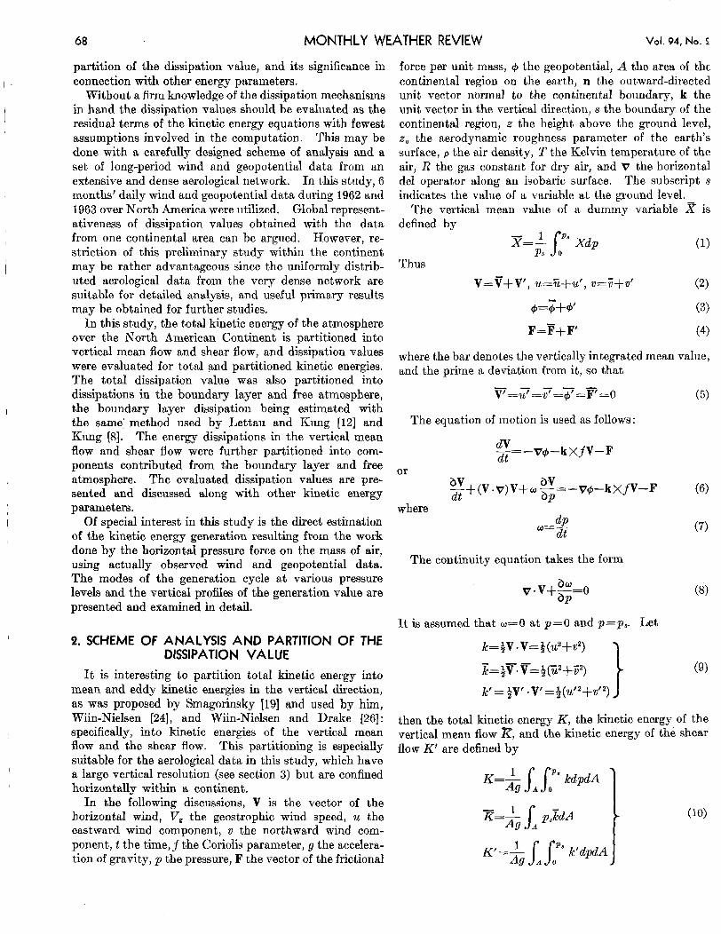
Figure 1 shows the distribution of the aerological stations. A total of 101 stations are on or within the continental boundary. An additional 18 stations outside the boundary were also used in computing horizontal partial derivatives for the stations on or near the boundary.

The computation was carried out on a daily basis. The data of each first day of the month were not included except to compute time derivatives for the next day. The days with relatively few available stations were excluded from the discussions of the following sections. The number of available stations within the continental region and the number on the boundary are shown in table 1 for each day except for those days excluded from the discussions. The table also shows the number of days available for each month; the monthly value of the computed results will be averaged from computed results for those individual days. An extremely strong cyclone pre- vailed over the continent during the latter two-thirds of


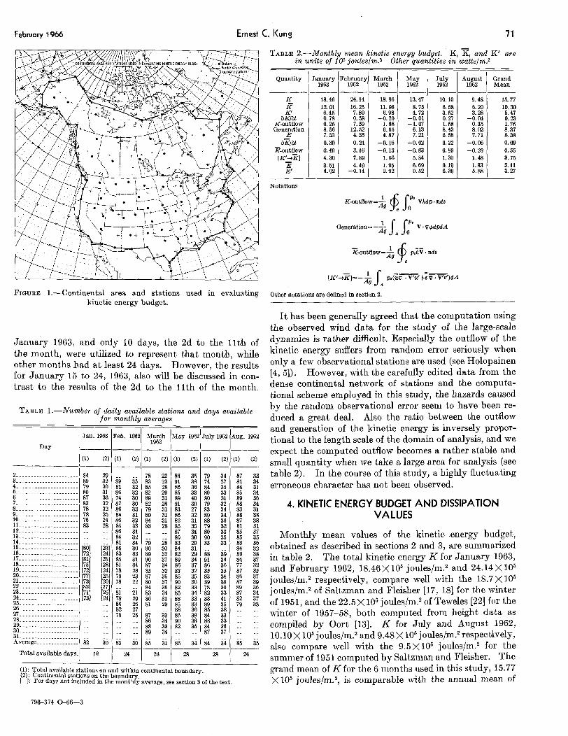
TABLE 2.-Monthly mean kinetic energy budget. X, 3, and K‘ are in uni t s of lo5 jouleslm.2 Other quantities in wattslm.2

July 1962

10.10 6.58 3.52 0.27 1.58 8.43 6.58 0.22 0.89 1.30 0.19 6.39

FIGURE 1.-Continental area and stations used in evaluating kinetic energy budget.

August 1962 --

9.48 6.20 3.28

-0.04 0.35 8.02 7. 71

-0.06 -0.29

1.48 1.83 5.88

January 1963, and only 10 days, the 2d to the 11th of the month, were utilized to represent that month, while other months had a t least 24 days. However, the results for January 15 to 24, 1963, also will be discussed in con- trast t o the results of the 2d to the 11th of the month.

x’ K’

bK/&t If-outflow Generation

E

TABLE 1.-Number of daily available stations and days available

12.01 16.25 11.98 8.75 6.45 7.89 6.98 4.72 0.78 0.58 -0.20 -0.01 0.25 7.59 1.88 -1.07 8.56 12.52 6.55 6.13 7.53 4.35 4.87 7.21

aZiat ?&UtA_ow [K’-)Kl

E E’

f o r monthly averages

0.30 0.24 -0.16 -0.02 0.49 3.16 -0.13 -0.83 4.30 7.89 1.66 5.84 3.51 4.49 1.95 6.69 4.02 -0.14 2.92 0.52

.. _. 89 35 81 32 86 32 74 30 87 30 86 33 84 31 86 32 84 33 86 31 84 32 81 34 85 30 83 33 85 31 81 34 78 28 79 23 78 22

81 21 78 29 86 26 82 27 79 25

._ ._

-. ._ - _ .. . . . . .... 83 30

24

Day

2 ...................... 3 4 ...................... 5 ...................... 6 ...................... 7. ..................... 8 ...................... 9. ..................... 10 ..................... 11 ..................... 12. ........................ 13 ......................... 14. ........................ 15 ..................... 16 ..................... 17 ..................... 18 ..................... 19 ..................... 20 ..................... 21 ..................... 22 ..................... 23.. ................... 24 ..................... 25 ......................... .......................... 27. ........................ 28.. ....................... 29. ........................ 30.. ....................... 31.. ....................... Average ...............

Total available days.

...................... 78 22 83 23 85 28 82 29 89 31 82 28 79 31 89 31 &4 31 83 28

79 28 90 30 89 32 90 37 87 34 85 32 87 36 80 37 84 35 83 34 86 31 81 29

87 33 86 34 88 33 89 34

85 31

. . . .

._ ..

. . . .

. . . .

Jan. 1963

(1) (2) --

84 29 89 32 79 30 80 31 87 36 83 32 78 32 78 25 76 24 83 28

801 [23 [721 [24 811 [25 [75] [28

[77] (731 821 (27

1721 .[24

[71] 1731 /2

82 30

10 -_

26

86 35 91 38 86 36 85 33 89 40 91 39 83 27 86 32 82 31 85 35 87 34 80 30 83 29 84 31 82 29 89 34 86 37 83 32 85 35 90 36 82 33 85 34 88 33 85 33 88 36 86 38 90 36 82 35

86 34

. . . .

.. ~.

28

79 34 74 27 84 35 80 33 80 31 79 32 83 34 89 34 88 36 79 32 80 33 90 35 83 33

88 39 91 34 86 36 85 35 83 34 89 38 78 30 82 33 88 41 89 35 85 38 84 33 88 33 84 36 87 37

84 34

. . . .

. . . .

28

(1): Total available stations on and within continental boundary. (2): Continental stations on the boundary. I I: For days not included in the monthly average, see section 3 of the text.

87 33 81 34 84 31 85 34 89 36 88 34 83 31 88 38 87 38 81 31 85 37 85 35 88 36 84 32 89 38 84 37 77 32 87 35 86 37 87 39 89 36 87 34 82 37 79 33 .- .. .. -. .- _. .. -. .- -. . . . . 85 35

24

Quantity January February March i 1963 1 1962 1 1962 1 K 18.46 24.14 .18.96 13.47

_ - ~ ~ - -

Other notations are de6ned in section 2.

Grand Mean

15.77 10.30 5.47 0.23 1.76 8.37 6.38 0.09 0.55 3.75 3.11 3. n

It has been generally agreed that the computation using the observed mind data for the study of the large-scale dynamics is rather difficult. Especially the outflow of the kinetic energy suffers from random error seriously when only a few observational stations are used (see Holopainen [4, 51). However, with the carefully edited data from the dense continental network of stations and the computa- tional scheme employed in this study, the hazards caused by the random observational error seem to have been re- duced a great deal. Also the ratio between the outflow and generation of the kinetic energy is inversely propor- tional to the length scale of the domain of analysis, and we expect the computed outflow becomes a rather stable and small quantity when we take a large area for analysis (see table 2). In the course of this study, a highly fluctuating erroneous character has not been observed.

4. KINETIC ENERGY BUDGET AND DISSIPATION VALUES

Monthly mean values of the kinetic energy budget, obtained as described in sections 2 and 3, are summarized in table 2. The total kinetic energy K for January 1963, and February 1962, 18.46 X lo5 joules/m.2 and 24.14 X lo5 joules/m.2 respectively, compare well with the 18.7 x lo5 joules/m.2 of Saltzman and Fleisher [17, 181 for the winter of 1951, and the 22.5X105 joules/m.2 of Teweles [22] for the winter of 1957-58, both computed from height data as compiled by Oort [13]. K for July and August 1962, 10.10X lo5 joules/m.2 and 9.48 X lo5 joule~/m.~ respectively, also compare well with the 9.5X105 joules/m.2 for the summer of 1951 computed by Saltzman and Fleisher. The grand mean of K for the 6 months used in this study, 15.77 X lo5 joules/m.2, is comparable with the annual mean of

798-374 0-66-3


-10

-m

-10 - -

- DAILY V I R I I I W O T K I N t l l C E t C R G Y CLNOATION. -:fi,p)&&ANO WTRW. V L 3%.0VIRmEI*IRW IMB(Ic*N coyI1”T -

- f - -

\ \ I I I I I I I I I I I I I I I I I I I I I I 1 ) 1 ) )

14.1 X lo5 joules/m.2 computed by Saltzman and Fleisher for the year 1951. The grand means of mean flow kinetic energy and shear flow kinetic energy K‘ are 10.30X lo6 joules/m.2 and 5.47 X lo5 joules/m.2 respectively. An approximate ratio of 2:l between and K‘ is observed for all 6 months.

Evaluated terms of the total kinetic energy equation (12), with the notation of table 2, should have the relation- ship :

E = - (bK/bt + K-ou tflow - genera tion)

In obtaining the total dissipation E, the important terms are those of the generation due to pressure forces, and the outflow of the kinetic energy from the continent; the local change of total kinetic energy dK/dt is one order of magnitude smaller. The grand means of bK/bt, K-outflow, and generation are 0.23, 1.76, and 8.37 watts/m.2 respectively.

Figure 2 shows the daily variation of the generation and

outflow terms of the kinetic energy. It seems that there is a correspondence between the generation and outflow.

Generally the North American continent is an area of horizontal divergence of the kinetic energy flux. If the difference of generation due to the horizontal pressure force and outflow is regarded as ((net generation” or “net supply” in the continental area, net generations thus obtained for January 1963 and February, March, May, July, and August 1962 are 8.31, 4.93, 4.67, 7.20, 6.85, and 7.67 watts/m.2 respectively, with a grand mean of 6.61 watts/m.a These net generation values for the continent are of the same order of magnitude as the conversion rate of available potential energy to kinetic energy, 0.91-3.37 watts/m.a as compiled by Oort [13]. His compilation was made of estimates by Brown [2], Krueger, Winston, and Haines [7], Saltzman [15], Saltzman and Fleisher [16, 171, Teweles [22], and Wiin-Nielsen, Brown, and Drake [25] from height data, and of results obtained by Phillips [14] and Smagorinsky [19] in their numerical experiments. That the net generations in this study are generally higher than the compiled conversion values may be explained in two ways. Firstly, this study is confined within the North American continent, and we may expect the generation in this region to be larger than the hemispherical average even after subtracting the outflow. An estimate of energy conversion over the same continent for January 1953 by White and Saltzman [23], 5 watts/m.2, compares well with the corresponding net generation values in this study. They used large-scale variations of individual pressure change and 500-mb. temperatures, and confined their study between latitudes 35’N. and 60°N. and longitudes 7OOW. and 120OW. Secondly, the use of both observed wind and height data at 20 pressure levels reveals a rather large kinetic energy generation due to the horizontal pressure force in the upper and lower troposphere over the continent (see table 5 and figs. 9 through 12); this will be discussed in detail in section 5.

The horizontal gradient field of 4 was obtained satis- factorily at all pressure layers, but the vertical integration of the geopotential 4 presents a problem. Since 4 in the upper troposphere is two orders of magnitude larger than that in the lower troposphere, a slight observational error of the pressure height in the upper levels may seriously obscure the significance of estimated 5. In this preliminary study, it is tentatively assumed that the term in the kinetic energy equation of the vertical mean

flow (13) which involves 5, (l/Ag)J p J VJdA, is negligible. This may be seen to a certain degree from the relation

A

- - -- - v . vl$=v. vl$-lpv*v

where v . ~ c $ may be as small as K-outflow (see table 2) and $ V . a should be very small as can be seen from the continuity equation (8).

Using the estimated terms of the mean flow kinetic


E Eb

- E, E E: Eb EI

E’ b E’/

Eb/E (%)

- - -

energy equation and the notation of table 2, equation (13) may be approximated by

7.53 2.41 5.12 3. 51 4.02 0.64 2.87 1.77 2.25 32.0

The most significant term in this equation is

TABLE %.-Total and partitioned kinetic energy dissipation (wattslm.2)

Quantity 1 January 1963

4.44 2.36 6.46 -0.10 1.82 2.97

-1.32 5.18 4.48 1. 64 43. 7 39.0 28.7. 22.8 18.3 29.1

-;::: I 2.2.; I 1.84 1 1.21 1 1.40 I 1.73

which, as discussed by Wiin-Nielsen [24], should essentially measure the kinetic energy conversion between the vertical shear and mean flows, a positive value showing the conversion from the shear flow to the mean flow. The grand mean of the conversion [K’+m is 3.75 wattslm.2 in comparison with the grand means of the dE/di, and E-outflow, which are 0.09, and 0.55 watts/m.2 respectively. The monthly value of [K’d?] varies from 1.30 to 7.89 watts/m.’ as listed in table 2. Smagorinsky [19], in his numerical experiment, obtained 1.61 wattslm.’ for the energy conversion from the vertical shear to the vertical mean flow. Wiin-Nielsen and Drake [26] gave 2.1 watts/m.2 for theh calculation with five months’ height data a t five pressure levels: 850, 700, 500, 300, and 200 mb. It is also noted that their original conversion values, before modifications, for January, April, July, and October 1962, and January 1963 are 4.65, 2.88, 1.24, 2.96, and 4.16 watts!m.’ respectively, which compare well with the [K’-g] values in this study listed in table 2. As a whole, conversion values from this study are higher than Smagorinsky’s [19] and Wiin-Nielsen’s and Drake’s [26] results; however, the differences in re- gions studied, vertical resolution, computation scheme, and type of data, should be considered.

We recognize that the kinetic energy converted from the available potential energy first takes the form of the vertical shear-flow kinetic energy, and then is converted to that of the vertical mean flow (see Smagorinsky [19] and Wiin-Nielsen [24]). The ratio of the conversion [K‘+a, 3.75 watts/m.2, to the net generation, 6.61 watts/m.2, within the continental region in this study is 0.57, which indicates that about 57 percent of the created kinetic energy eventually goes into the vertical mean flow. This ratio was about 0.68 in Smagorinsky’s [19] numerical experiment, about 0.27 in Wiin-Nielsen’s [24] earlier estimation, and was 1 .OO in Wiin-Nielsen’s and Drake’s [26] more recent study with their lowest conversion value between shear and mean flows. Both quantities involved in this ratio, especially kinetic energy generation, have been estimated by various investigators in diverse ways using different data, resulting in a wide range of numerical values. For this reason the author preferred t o use a set of values from this study only.

The total dissipations E, computed as the residual in the total kinetic energy equation (12), for January 1963 and February, March, May, July, and August 1962 (see

tables 2 and 3) are 7.53, 4.35, 4.87, 7.21, 6.58, and 7.71 watts/m.’ respectively, with a grand mean of 6.38 watts/ m.2 The mean flow dissipations E for these months, computed as the residual in the vertical mean flow kinetic energy equation (13) tentatively dropping terms (1,Ag)S pJ-v$dA as discussed earlier, are 3.51, 4.49,

1.95, 6.69, 0.19, and 1.83 watts/m.2 respectively, with a grand mean of 3.11 watts/m.2 The vertical shear flow dissipations E‘, obtained as the differences of E and E for the same respective months, are 4.02, -0.14, 2.92, 0.52, 6.39, and 5.88 wattsjm.2, with a grand mean of 3.27 watts/m .2

I t is noted that the total dissipation E is rather large, or at least not necessarily small, for July and August 1962. This is due to large generation values in the upper troposphere during the summer months (see figs. 9, 10, and 11, and table 5) .

Two things might be pointed out in connection with the dissipation values of the vertical mean flow, E. First, though E is primarily dependent on the magnitude of the conversion [K’+m in balancing equation (13), z-outflow also is not negligible. Second, though in general we may expect the vertical mean wind and frictional force F to tend to oppose each other, giving a positive dissipation, this tendency may not necessarily show up in a continental area for a monthly period, resulting in a negative monthly E .

The dissipations in the mean and shear flows, E and E’, are 49 percent and 51 percent of the total kinetic energy dissipation, while the kinetic energies a and K’ contained in the mean flow and shear flow are 65 percent and 35 percent of the total energy respectively. In other words, the ratio E/E‘ is 0.95; this ratio was 0.38 in Wiin- Nielsen’s [24] earlier estimate, and 2.24 in Smagorinsky’s [19] numerical experiment.

The energy dissipations in the boundary layer, Et,, (see table 3) computed with equations (15) through (20), for January 1963 and February, March, May, July, and Au- gust 1962 are 2.41, 1.90, 1.90, 2.07, 1.50, and 1.41 watts/m.’ respectively with a grand mean of 1.87 watts/m.’ Kung [SI, by the same method, but with the 1000-mb. geostrophic wind speed at 360 diamond grid points from latitudes 25O to 70° N. over the Northern Hemisphere, obtained Eo over North America for winter, spring, sum-

A

-

74 MONTHLY WEATHER REVIEW Vol. 94, No, 2

E 6. 38

E, 1. 87

mer, and fall for the period 1945 t o 1955 as 2.43, 2.09, 1.22, and 2.03 watts/m.2 respectively, with an annual mean of 1.94 watts/m.2 The hemispherically averaged E, values in the same study for the corresponding seasons are 1.94, 1.33, 0.70, and 1.40 watts/m.2 respectively with an annual mean of 1.34 watts/m.2 Lettau [lo] estimated frictional energy dissipation below the 700-mb. level to be 1.4 watts/m? using zonal means of the 700-mb. level wind speed and ground drag.

The ratio Eb/E is interesting since it expresses the portion of the total energy dissipation that takes place in the boundary layer and consequently whether the dissipation in the free atmosphere is as important as in the boundary layer. The percent ratios Eb/E as listed in table 3 are 32, 44, 39, 29, 23 and 18 percent for January 1963 and Feb- ruary, March, May, July, and August 1962 respectively

The ratio of the boundary layer dissipation to the total dissipation is smaller in the summer months than in the winter months and this may be attributed to two factors: the relatively large kinetic energy generation in the upper troposphere, and the weaker geostrophic wind speed and consequent weaker dissipation in the lower troposphere in the summer though the earth’s surface roughness is a t its peak. The difference of E and Ea should estimate the dissipation in the free atmosphere, E,; as shown in table 3 the E, values obtained for the above 6 months are 5.12, 2.45, 2.97, 5.14, 5.08, and 6.30 watts/m.2 with an annual mean of 4.51 watts/m.?, which in turn means that 68, 56, 61, 71, 77, and 82 percent of the total dissipation for the individual months and 71 percent of the grand mean total dissipation took place in the free atmosphere. However, it should be remembered that the thickness of the planetary boundary layer is only about 100 mb., and in turn the dissipation should occur more intensely in the boundary layer than in the free atmosphere. If the thickness of the boundary layer and free atmosphere are taken as 100 mb. and 900 mb., the dissipation should be 18.7 ergs set.-' cm.-*mb.-’ in the boundary layer and 5.0 ergs set.-' cm.-2mb.-1 in the free atmosphere respectively on the annual mean basis.

Brunt’s [3] early estimation of 3 watts/m.2 for the energy dissipation below 1 km. is 60 percent of his estimation of total dissipation, 5 watts/m.2 Jensen [6] estimated the energy dissipation in the 1000- t o 925-mb. layer for January 1958 over the Northern Hemisphere north of 20’ N., as 3.36 watts/m.2, and in the layer of 1000 t o 50 mb. as 4.28 watts/m.2, giving the ratio of the former to the latter as 78 percent. Holopainen [4] estimated the dissipation in the layer from surface to 900 mb. over the British Isles, for January 1954, as 4.2 watts/m.2 and in the layer from the surface to 200 mb. as 10.4 watts/m.2, indicating that 40 percent of the total dissipation was in the layer below 900 mb. In his later paper, Holopainen [5] estimated the dissipation below 800 mb., also over the British Isles and for Septem- ber, October, and November 1954, as 5.2 watts/m2. and the dissipation in the layer of 1000 mb. to 200 mb. as only

j with a ratio for the grand mean values of 29 percent.

I

E E’ 3. 11 3. 27

B b E’ b 0. 14 1. 73

1.9 watts/m.a The obvious discrepancy between his earlier and later results may be due to probable errors in evaluating the kinetic energy equation for the upper troposphere, as pointed out by Holopainen [5] himself, and/or confinement of his study to a small area, as discussed in section 3. It is difficult, however, to confirm the nature of the discrepancy in his results because of the possible involvement of the regional and seasonal charac- teristics.

Further partitions of the dissipation values obtained in this study into Zb, Z,, E : , and E;, as discussed in section 2, are listed in table 3. The portion of the mean flow dissipation contributed by the boundary layer ,To, is very small, and unless the mean flow dissipation E itself is very small the major portion of E is due to that contributed from the free atmosphere, The shear flow dissipation contributions from the boundary layer and free atmosphere, El and E; are of the same order of magnitude on an average. However, when Z? is significantly larger than E’ as in February and May 1962, the major part of E’ is the contribution from the boundary layer, E:. Also, as a gross feature, it may be stated that the major portion of the boundary layer dissipation, E,,, contributes to the shear flow dissipation, while the free atmosphere dissipation, E,, contributes substantially to both the mean flow and shear flow dissipations. The grand means of the above dissipation values may be summarized according t o the partitioning table in the last paragraph of section 2 (unit in watts/m?.):

As described in section 3, only 10 days data from Jan- uary 2 to 11, 1963, were used to represent that particular month as an ordinary winter month. It is of some interest to compare some results obtained for that period with those for another 10-day period, the 15th to the 24th of the same month, when an extremely strong cyclone persisted over most of the North American continent. As shown in table 4, when the weather pattern was extremely cyclonic (January 15-24), the total energy level, K, almost doubled, and the ratio of mean flow energy level, x, to the shear flow energy level, K’, seemed to increase too. The most outstanding feature of the energy budget during strong cyclonic activity was the tremendous increase of the generation and outflow of the kinetic energy (also see fig. 2) while the net generation for the continent (generation minus outflow) actually got smaller. Ap- parently the continental region served as the important supplier of kinetic energy to the North Atlantic Ocean during that period. In connection with this, it should be noted that during that period the boundary layer dissipation Ea increased a little from stronger winds, but the


TABLE 4.-Kinetic energy budget and dissipation in early and late periods of January 1963. K , E, and K' are in uni ts of 105 joules/ma; other quantities in wattslm.2 Notation i s as defined in section 1 and table 1.

Period

Jan.15-24 Jan. 2-11 _________._ _ _ _ _ _ _ _ _ _ ~ 3 5 . 4 8 ~ 2 5 . 1 4 ~ 1 ~ ~ ~ ~ 18.46 12.01 i:gl 4.30 2.4214.9612.551 7.53 2.41 5.12 2.41

free atmosphere dissipation, E,, decreased significantly, even giving a rather small total dissipation. It is not an unreasonable speculation that the enormous kinetic energy created over the continent would, be dissipated over the ocean after it flowed out.

5. VERTICAL PROFILE OF KINETIC ENERGY GENERATION

In the kinetic energy equation (12), the term

-& V.v$dpdA

stands for the generation of kinetic energy from the work done by the horizontal pressure gradient on the mass of the atmosphere over the regibn. This is regarded as the source term in the kinetic energy equation. The corresponding quantity per unit mass of air can be written

(37) - v . v4 = -VI v+-- __ - w a

where a is the specific volume. If equation (37) is integrated over the entire mass of the atmosphere M, we

as

bP

obtain n n

which should represent the conversion to the kinetic energy from the total potential (i.e., the potential plus internal) energy (see White and Saltzman [23]). Thus, the generation of kinetic energy is customarily measured by the integration of w a for studies of hemispherical or global scale. Nevertheless, in practice, the estimate of vertical p-velocity, w, involves a great deal of dif6culty and controversy. Moreover, if the kinetic energy generation is to be obtained for a portion of the atmosphere, the integrals of all three terms a t the right side of (37) must be computed rather than the right side of (38) ; none of them is easily done.

The direct estimation of the kinetic energy generation by -V .VC$ with actually observed wind and geopotential data is by no means an easy task since the necessary determination of the geopotential gradient at each station is very difficult. However, the directness of the term -V .V+, in the physical sense and in the analysis of the observed meteorological data is appealing. The kinetic energy is created from the potential energy through the work done on the mass of air by the horizontal pressure

force when there is a component of flow in the negative direction of t'he geopotential gradient.

The usefulness of the study of the kinetic energy generation by the direct estimation of -V .VC$ was suggested by Smith [21] as early as 10 years ago, but investigations along this line received little attention except from Holopainen [4, 51.

In this study, employment of a method, as discussed in section 3, of evaluating the geopotential gradient a t individual stations with data from the dense continental network of observations seems to yield interesting vertical distributions of the generation term -V . ~ 4 . Thegenerclr tion of kinetic energy within each 50-mb. pressure layer,

- l / g s p ' P1 V-V4dp, where p2-p,=50 mb., is averaged over

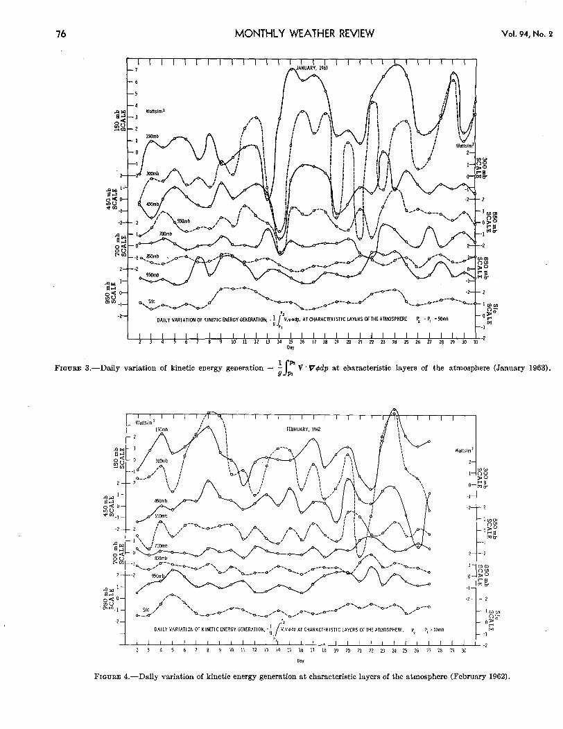
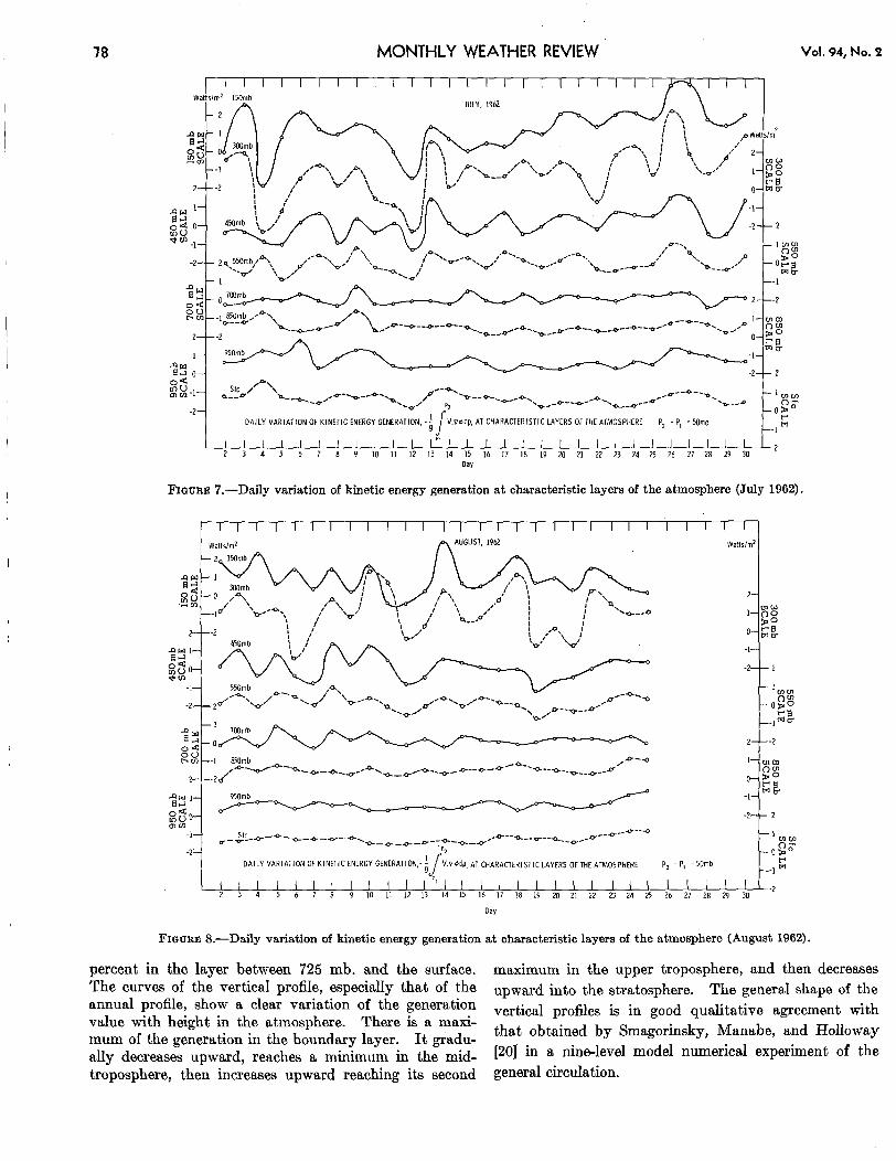
the continental region and presented as follows. Figures 3 through 8 show the daily variation of the

kinetic energy generation in eight 50-mb. pressure layers of the atmosphere, centered a t 150, 300, 450, 550, 700, 850, and 950 mb., and surface layer whose lower boundary is the surface pressure, for January 1963 and February, March, May, July, and August 1962. As far as the kinetic energy generation due to the horizontal pressure force is concerned, there seem to exist three cyclic modes in the vertical direction of the troposphere. In the upper troposphere the amplitude of fluctuation of the generation is very large both in plus and minus directions, and a cyclic appearance of the maxima or minima in long periods of the order of 10 days is observed. Apparently the characteristic shape of the time sequence of the generation for the entire, depth of atmosphere, which is shown in figure 2, is mainly contributed to from the upper troposphere fluctuations. In the mid-troposphere the generation values are smaller than in the upper troposphere; the generation also fluctuates in both plus and minus directions, but with much smaller amplitude. The appearance of the maxima or minima in the long periods observed at the higher levels is still traceable, but is somewhat obscured by the cycle of the short periods of the order of a few days. In the lower troposphere, the generation is large, of the same order of magnitude as in the upper troposphere, but the fluctuations are the smallest of the three parts of the troposphere. We also notice that the generation value is almost constantly positive in the lower troposphere. This is reasonable since in the lower troposphere the component of the cross-isobar flow is in the negative direction of the pressure gradient due to friction giving a positive value to - V VQ

Table 5 contains monthly means of kinetic energy generation in each 50-mb. pressure layer for the six sampled months and their grand mean. I n plots of these values in figures 9 through 12, the values for the pressure layer 1025-975 mb. are substituted for those of the surface layer because wind data at the 1OOO-mb. level usually exist only at less than half of the available stations in the continental region. Figure 9 shows vertical profiles of the generation for January 1963 (both


,.o--*--.Y' '\ h.4. -**-*e--*.. 'a--o--4

-0-0. =. % .p -- ---

DAILY VARIATION OF KINETIC ENERGY GENERATION, - m AT CHARACTERISTIC LAYERS OFTHE ATMOSPHERE p? - -50mb

Day

FIGURE 3.-Daily variation of kinetic energy generation - A V ' V&p at characteristic layers of the atmosphere (January 9 s PI 1963).

FIGURE 4.-Daily variation of kinetic energy generation at characteristic layers of the atmosphere (February 1962).

February 1966 Ernest C. Kung

DAILY VARIATION OF KINETIC ENERGY GENERATIDN,-1 V .Wdp,AT CHARACTERISTIC LAYERS OF ATMOSPHERE p2 - PI 50mb J -2 -

77

- - - I

---2

1 1 1 1 1 1 1 1 1 1 1 1 1 1 1 1 1 1 1 I I I I I I I I I I

p m ' 2

May 1962

1-

2--2

-2-- 2

~--~--~--*--*--~--*--~,,*-.~--o--o-----*~~ SIC

2-

-1

I I I I I I I I I I I I

Day

FIGURE 6.-Daily variation of kinetic energy generation at characteristic layers of the atmosphere (May 1962).

January 2-11 and 15-24 periods) and February 1962, which may be regarded as the winter profiles; figure 10 shows profiles for March and May 1962, which may be regarded as the spring profiles; figure 11 shows profiles for July and August 1962 which may be regarded as the summer profiles; and figure 12 shows the profile for the grand mean, which may be regarded as the annual profile.

I t is obvious, by looking a t these figures, that strong generation takes place in the upper and lower troposphere while the generation in the mid-troposphere is very weak. On the annual basis, by taking the surface level as 1000 mb., it may be estimated that roughly 46 percent of the total generation is in the layer between 75 and 425 mb., 8 percent in the layer between 425 and 725 mb., and 46


t

- 2 t

FIGURE 7.-Daily variation of kinetic energy generation at characteristic layers of the atmosphere (July 1962).

FIGURE 8.-Daily variation of kinetic energy generation at characteristic layers of the atmosphere (August 1962).

percent in the layer between 725 mb. and the surface. The curves of the vertical profile, especially that of the annual profile, show a clear variation of the generation value with height in the atmosphere. There is a maximum of the generation in the boundary layer. It gradu- allv decreases uDward. reaches a minimum in the

maximum in the upper troposphere, and then decreases upward into the stratosphere. The general shape of the vertical profiles is in good qualitative agreement with that obtained by Smagorinsky, Manabe, and Holloway [20] in a nine-level model numerical experiment of the

troposphere, the; increases upward reaching its second general circulation.

February 1966 Ernest C. Kung mb 100

150

200

250

300

350

400

450

500

550

600

650

700

750

800

850

900

950

P

I I I I I mbl I I I I - - - -

- - - - - - - - - - - - - -

FIGURE 9.-Monthly vertical profile of kinetic energy generation (January 1963 and February 1962).

mb

100

150

200

250

300

350

400

450

500

550

600

650

700

750

8M)

850

900

950

Surface

P

I I 7 - - - - - - - - - - - - - - - - - -

-0.5

mb 100

150 - 200

250 - 300 - 350 - 400 - 450 - 500 - 550 - 600

650 - 700 - 750 - 800

850 - 900 - 950 -

Surface

-

-

P

-

-

I

79

t 1 I 4 MONTHLY VERTICAL PROFILE OF I ENERGY GENERATION

j I

t t

K I NET1 C

I 2% I I I I -0.5 0 0.5 1.0 1.5 2.0 2.5 Watts/m2

FIGURE 11 .-Monthly vertical profile of kinetic energy generation (July and August 1962).

1 I I 1 I 1

FIGURE 12.-Mean vertical profile of kinetic, energy generation.

798-374 0-66-4


Lugust 1962

0.77 0.82 0.62 0.63 0.53 0.35 0.23 0.16 0.15 0.19 0.17 0.12 0.11 0.37 0.63 1. 07 1.00 0.74 0.90 0.26

TABLE B.-Monthly mean kinetic energy generation (watts m.-2 (60 nib.)-' (watts m.-2 (60 mb.)- l ) within each pressure layer

Grand Mean

--.- 0.95 1.24 1.20 0.96 0.67 0.44 0.34 0.21 0.13 0.09 0.09 0.10 0.10 0.32 0.48 0.72 0.77 0.68 0. 72 0.41

- 0.81 0.74 1.34 0.90 0.74 0.51 0.44 0.32 0.31 0.22 0.13 0. 07 0.04

-0.08 0.39 0.51 0.13 0.19 0.47

-0. 04

1.33 2.79 1.82 1.48 0.80 0.48 0.30 0.21 0.11 0.01 0.09 0.13 0.02 0.67 0.71 0.31 0. 66 0.47 0.18 0.09

-- 0.70 0.73 0.74 0.73 0.59 0.44 0.24 0.06

-0.02 -0.07

0.03 0. 06 0.18 0. 26 0.43 0.84 0.93 1.20 1.29 0.37

I

pebruary March 1962 I 1962

1.08 1.05 1.19 1.19 1.42 1.26 1.02 0.99 0.65 0.72 0.40 0.49 0.43 0.39 0.20 0.32 0.19 0.05 0.14 0. MI 0. 07 0.03 0.13 0.08 0.35 -0.12 0.59 0. 13 0.75 0.07 1.41 0. 18 1.59 0.34 1.11 0.39 0.93 0.56 1.24 0.57

The vertical profiles of the generation shown in figures 9, 10, and 11 seem to show a seasonal variation. The winter profiles in figure 9 show strong generation both in the upper and lower troposphere. During the vigorous cyclonic period of January 15-24, 1963, extremely strong generation a t the tropopause level was significant. Spring profiles in figure 10 show that upper troposphere generation was weakened while the lower troposphere generation was still strong. Summer profiles in figure 11 show that the upper troposphere generation strengthened again while the lower troposphere generation became weak. How- ever, proliles from six months data are not enough to give conclusive definition of a seasonal variation.

Since the kinetic energy dissipation E is mainly balanced by the generation term for a long-term grand mean (see table 2), the general shape of the annual vertical profile of the dissipation should follow that of generation shown in figure 12.

6. KINETIC ENERGY GENERATION AND DISSIPATION IN THE BOUNDARY LAYER AND FREE ATMOSPHERE

There are two reasons, we may speculate, that the kinetic energy dissipation in the boundary layer is largely balanced by the generation in the boundary layer due to the horizontal pressure force. First, if we recognize an approximate balance of the horizontal pressure force, the Coriolis force, and the frictional force in the boundary layer, it should imply the same balance between the kinetic energy generation and the dissipation. Second, observational studies (see Holopainen [4, 51 and Jensen. [6] for examples) and numerical experiments (see Smagorinsky, Manabe, and Holloway [20]) indicate that the vertical transport of the kinetic energy a t or near the top of the boundary layer is very small in comparison with the generation in the boundary layer.

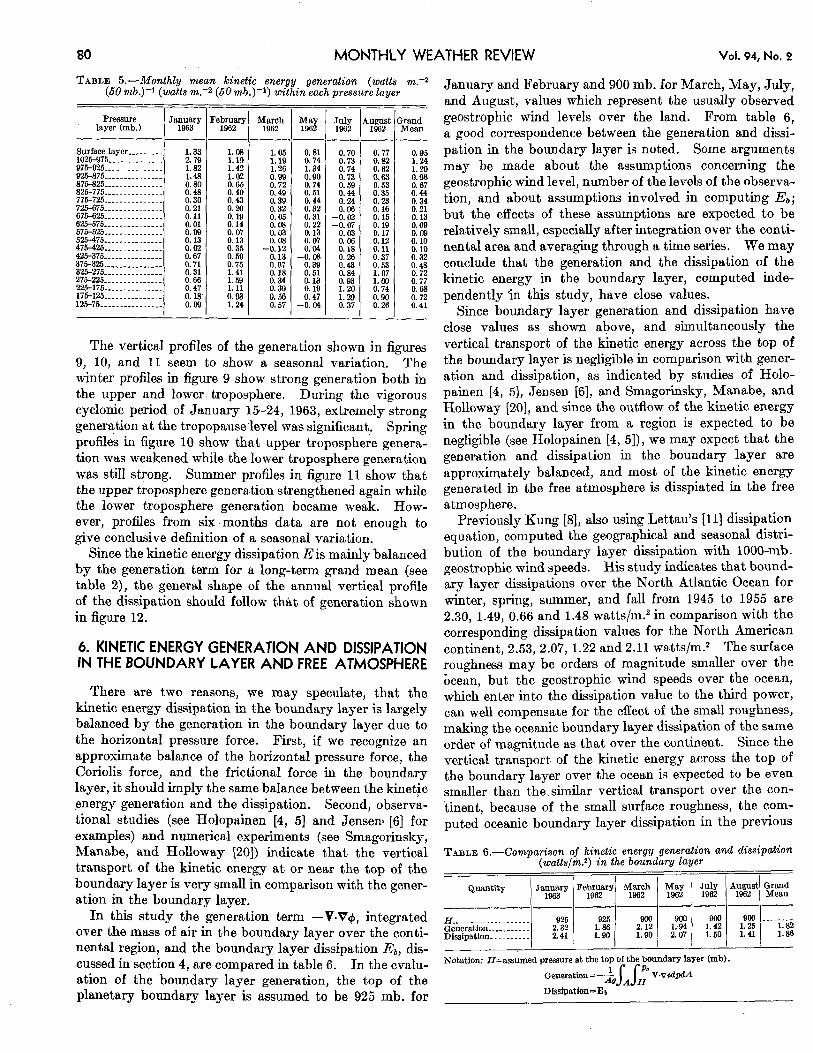
In this study the generation term -V.V4, integrated over the mass of air in the boundary layer over the continental region, and the boundary layer dissipation Ea, discussed in section 4, are compared in table 6. In the evaluation of the boundary layer generation, the top of the planetary boundary layer is assumed to be 925 mb. for

January and February and 900 mb. for March, May, July, and August, values which represent the usually observed geostrophic wind levels over the land. From table 6, a good correspondence between the generation and dissipation in the boundary layer is noted. Some arguments may be made about the assumptions concerning the geostrophic wind level, number of the levels of the observa- tion, and about assumptions involved in computing Ea; but the effects of these assumptions are expected to be relatively small, especially after integration over the continental area and averaging through a time series. We may conclude that the generation and the dissipation of the kinetic energy in the boundary layer, computed independently *in this study, have close values.

Since boundary layer generation and dissipation have close values as shown above, and simultaneously the vertical transport of the kinetic energy across the top of the boundary layer is negligible in comparison with generation and dissipation, as indicated by studies of Holo- painen [4, 51, Jensen [6], and Smagorinsky, Manabe, and Holloway [%I], and since the outflow of the kinetic energy in the boundary layer from a region is expected to be negligible (see Holopainen [4, 5]), we may expect that the generation and dissipation in the boundary layer are approximately balanced, and most of the kinetic energy generated in the free atmosphere is disspiated in the free atmosphere.

Previously 'Rung [8], also using Lettau's 1111 dissipation equation, computed the geographical and seasonal distribution of the boundary layer dissipation With 1000-mb. geostrophic wind speeds. His study indicates that boundary layer dissipations over the North Atlantic Ocean for winter, spring, summer, and fall from 1945 to 1955 are 2.30, 1.49, 0.66 and 1.48 watts/m.2 in comparison with the corresponding dissipation values for the North American continent, 2.53, 2.07, 1.22 and 2.11 watts/m.2 The surface roughness may be orders of magnitude smaller over the bcean, but the geostrophic wind speeds over the ocean, which enter into the dissipation value to the third power, can well compensate for the effect of the small roughness, making the oceanic boundary layer dissipation of the same order of magnitude as that over the continent. Since the vertical transport of the kinetic energy across the top of the boundary layer over the ocean is expected to be even smaller than the,similar vertical transport over the continent, because of the small surface roughness, the computed oceanic boundary layer dissipation in the previous

TABLE 6.-Comparison of kinetic energy generation and dissipation (wattslm.2) in the boundary layer

Quantity January February March May July August Grand 1 1963 1 1962 I 1962 1 1962 I 1962 1 1962 1 Mean

H __..._._._.__.____ 925 1 925 1 900 1 900 1 900 1 9W I--------

Generation.. _ _ _ _ _ _ _ _ _ 2.32 1.86 2.12 1.94 1.42 1.25 1.82 Dissipation ___..___ _ _ 2.41 1.00 1.90 2.07 1.50 1.41 1.86

I 1 I I , 8

Notation: H=assumed pressure at the top - of c the rn boundary layer (mb).


study [8] should be nearly equivalent to the oceanic boundary layer generation.

7. CONCLUDING SUMMARY AND REMARKS As a preliminary of a systematic study of the kinetic

energy dissipation problem in the large-scale atmospheric circulation, the kinetic energy budget and dissipation values are studied in their various partitionings, using daily wind and geopotential observations from the network over the North American continent for six months.

The total kinetic energy dissipation of the atmosphere is partitioned into vertical mean flow and shear flow and also into boundary layer and free atmosphere. The total kinetic energy dissipation, E, and mean flow kinetic energy dissipation, E, are obtained separately as residual terms required to balance the total kinetic energy equation and the mean flow kinetic energy equation. The kinetic energy dissipation in the vertical shear flow, E’, is obtained as the difference of E and E. The kinetic energy dissipation in the planetary boundary layer E, is estimated using Lettau’s [11] universal wind spiral solution and roughness parameters evaluated by Lettau and Kung [12] and Kung [SI, and dissipation in the free atmosphere, E,, is obtained as the difference of E and E,. Further, I? is partitioned into the dissipation contributed by the boundary layer, Eb and that contributed by the free atmosphere, E,. In the same manner E’ is partitioned according to contributions from the boundary layer, E‘b, and from the free atmosphere, Erp

Since the observed wind data are used along with geopotential and other data, the horizontal partial derivatives of various quantities have to be evaluated a t individual stations. A special procedure to compute the horizontal gradient of a scalar quantity and the divergence of a vector field is designed, and applied in estimating various quantities in the kinetic energy equations.

The grand means of the total kinetic energy, K, mean flow kinetic energy, f??, and shear flow kinetic energy, K’, are 15.77X lo5, 10.30X lo5 and 5.47X lo5 joules/m.2 respectively, and an approximate ratio of 2 :1 between

and K‘ is recognized throughout all months observed. The grand means of the local change, outflow, and

generation, in the total kinetic energy equation are 0.23, 1.76, and 8.37 watts/m.2 respectively. There also seems to be a correspondence between the daily variations of generation and outflow. Generally the North American continent is shown as an area of horizontal divergence of kinetic energy flux. Especially during the period of strong cyclonic activity, the continent acts as an important supplier of kinetic energy to the North Atlantic Ocean. The difference of the generation and outflow, which is regarded as the net generation of the kinetic energy in the continental area, is comparable with the energy conversion rates obtained by other investigators. Some- what larger net generation values in this study, compared to others, are explained by the restriction of the study to a continent, and by the use of a large vertical resolution

of observed wind and height data (i.e., 20 isobaric levels from the surface to the 100-mb. level).

The kinetic energy conversion between the vertical shear and mean flows has the grand mean of 3.75 watts/m.2 for the six months used, showing that 57 percent of the net generation over the continent, which first takes the form of the vertical shear flow energy, eventually goes into the vertical mean flow. This quantity is the most significant term in the equation of the mean flow kinetic energy.

The total dissipation E, mean flow dissipation E, and shear flow dissipation E’ have the grand means of 6.38, 3.11, and 3.27 watts/m.2 respectively for the combined six months. Because of the large generation value in the upper troposphere in the summer, E is not necessarily small for July and August 1962. It is noted that the dissipations and E’ are 49 percent and 51 percent of the total dissipation while the energy components and K’ are 65 percent and 35 percent of the total kinetic energy. The grand means of the boundary layer dissipation Ea and free atmosphere dissipation E, for the six months are 1.87 and 4.51 watts/m.2 respectively, 29 percent of the total dissipation taking place in the boundary layer. During the summer a smaller portion of the total dissipation takes place in the boundary layer than during the winter because of a relatively strong generation in the upper troposphere and a relatively weak wind in the boundary layer, though the earth’s surface roughness is a t its maximum.

The further partitioned components of the dissipation Eo, E,, EL and E; have the grand means of 0.14, 2.97, 1.73, and 1.54 watts/m.2 respectively for the six months combined. Generally, the major portion of the mean flow dissipation is contributed from the free atmosphere, and the shear flow dissipation is contributed from the boundary layer and the free atmosphere in the same order of magnitude.

In this study the generation of the kinetic energy is directly evaluated as the quantity - V.V$J, generation due to the work done by the horizontal pressure force. Daily variations of the kinetic energy generation in various layers of the atmosphere are presented. There seem to be three modes of the generation cycle in the upper, mid, and lower troposphere. In the upper troposphere the amplitude of fluctuation is large in both plus and minus directions, and the long-period oscillation is significant. In the mid-troposphere the amplitude and period of the oscillation are much smaller than in the upper troposphere, but the fluctuations are still to both plus and minus directions. In the lower troposphere the generation is large; however, the fluctuation is the least for the three parts of the troposphere, and the generation is constantly positive because of the frictional effect. When the generation values are plotted for 50-mb. pressure layers from the surface to the 100-mb. level, interesting monthly and grand mean vertical profiles of the kinetic energy generation are obtained. Strong generation takes place in the upper and lower troposphere, while the generation in the mid-tropo-


sphere is very weak. Generation also seems to decrease rapidly into the stratosphere from the upper troposphere maximum. The variation of the generation with height is very clear and in good qualitative agreement with that obtained by Smagorinsky, Manabe, and Holloway [20] in their numerical experiment. There also seems to be a seasonal variation of the vertical profile of the generation. The general shape of the annual vertical profile of the dissipation is expected to resemble that of the grand mean of the generation.

The generation and the dissipation of the kinetic energy in the boundary layer computed independently in this study, along with some evidence from other investigators, suggest that there may be an approximate balance of the boundary layer generation and dissipation.

The grand mean values presented in this study for the six months, i.e., February, March, July, and August 1962 and January 1963, may be regarded as annual mean values.

Also because of the preliminary nature of this study, only data for the six months were analyzed; vertical distributions of energy parameters were not computed except for the generation term; and the regional and seasonal char- acteristics were not investigated in detail. These interesting points will be studied systematically in detail in the investigation currently in progress.

ACKNOWLEDGMENT The author is greatly indebted to Professor V. P. Starr of the

Massachusetts Institute of Technology, through whose courtesy parts of the aerological data were made available while the entire data were still in the stage of being processed. The kind assistance of Messrs. H. Frazier and S. F. Seroussi of the Travelers Research Center, Inc. is gratefully acknowledged.

The author would especially like to thank Dr. S. Manabe for his valuable suggestions and stimulating discussions which influenced the course of the study, and for later reviewing the manuscript.

The author wishes to express his sincere gratitude to Dr. J. Sma- gorinsky for his encouragement and suggestions, to Dr. Y. Kurihara for his very valuable suggestions and discussions, to Dr. K. Bryan for reviewing the manuscript, to Mr. S. Hellerman for kindly helping in a part of the data handling and later reviewing the original manuscript, and particularly to Mr. R. D. Graham for providing the necessary arrangements in various aspects of the study and later reviewing the manuscript. Many thanks are also due to Mrs. R. A. Brittain and Mrs. J. A. Snyder who helped in preparing the manuscript, to Mrs. E. J. Campbell who patiently assisted in data analysis, and to Mr. E. W. Rayfield and Mr. G. C. Reynolds who assisted in preparing the figures.

The valuable comments of Professors R. A. Bryson and D. R. Johnson of the University of Wisconsin are sincerely acknowledged.

REFERENCES 1. F. K. Ball, “Viscous Dissipation in the Atmosphere,” Journal of

Meteorology, vol. 18, No. 4, Aug. 1961, pp. 553-557. 2. J. A. Brown, “A Diagnostic Study of Tropospheric Diabatic

Heating and the Generation of Available Potential Energy,” Tellus, vol. 16, No. 3, Aug. 1964, pp. 371-388.

3. D. Brunt, Physical and Dynamical Meteorology, Cambridge University Press, 1939, 428 pp.

4. E. 0. Holopainen, “On the Dissipation of Kinetic Energy in the Atmosphere,” Tellus, vol. 15, No. 1, Feb. 1963, pp. 26-32.

5. E. 0. Holopainen, “Investigation of Friction and Diabatic Processes in the Atmosphere,” Paper No. 101, Dept. of Mete- orology, University of Helsinki, 1964, 47 pp.

6. C. E. Jenson, “Energy Transformation and Vertical Flux Process over the Northern Hemisphere,” Journal of Geo- physical Research, vol. 66, No. 4, Apr. 1961, pp. 1145-1156.

7. A. F. Krueger, Jay S. Winston, and D. A. Haines, ‘[Computation of Atmospheric Energy and its Transformation for the Northern Hemisphere for a Recent Five-Year Period,” Monthly Weather Review, vol. 93, No. 4, Apr. 1965, pp. 227-238.

8. E. C. Kung, Climatology of the Mechanical Energy Dissipation in the Lower Atmosphere over the Northern Hemisphere, Ph. D. Thesis, University of Wisconsin, 1963, 92 pp.

9. Y. Kurihara, “Numerical Analysis of Atmospheric Motions,”

10.

11.

12.

13.

14.

15.

16.

17.

18.

19.

20.

21.

22.

23.

24.

25.

26.

Journal of Meteorological Society of Japan, Series 11, vol. 6, Dec. 1960, pp. 288-304. H. H. Lettau, “A Study of the Mass, Momentum, and Energy Budget of the Atmosphere,” Archiv fur Meteorologie, Geophysik und Bioklimatologie, Series A, vol. 7, 1954, pp. 133-157. H. H. Lettau, “Theoretical Wind Spirals in the Boundary Layer of a Barotropic Atmosphere,” Beitrage zur Physik der Atmosphdre, vol. 35, No. 314, 1962, pp. 195-212. H. H. Lettau and E. C. Kung, “Aerodynamic Roughness of the Earth’s Surface: A Parameterization for Use in General Circulation Studies,” 1965 (Paper in preparation).

A. H. Oort, “On Estimates of the Atmospheric Energy Cycle,’’ Monthly Weather Review, vol. 92, No. 11, Nov. 1964, pp.

N. A. Phillips, “The General Circulation of the Atmosphere: A Numerical Experiment,” Quarterly Journal of the Royal Meteorological Society, vol. 82, No. 352, Apr. 1956, pp. 123-164. B. Saltzman, “The Zonal Harmonic Representation of the Atmospheric Energy Cycle-A Review of Measurements,” The Travelers Research Center, Report TRC-9, Sept. 1961, 19 PP. B. Saltzman and A. Fleisher, “Spectrum of Kinetic Energy Transfer Due to Large-Scale Horizontal Reynolds Stress,” Tellus, vol. 12, No. 1, Feb. 1960, pp. 110-111. B. Saltzman and A. Fleisher, “Further Statistics on the Modes of Release of Available Potential Energy,’’ Journal of Geophysical Research, vol. 66, No. 7, July 1961, pp. 2271-2273. B. Saltzman and A. Fleisher, “Spectral Statistics of the Wind a t 500 mb.,” Journal of the Atmospheric Sciences, vol. 19, No. 2, Mar. 1962, pp. 195-204.

J. Smagorinsky, “General Circulation Experiments with the Primitive Equations, 1. The Basic Experiment,” Monthly Weather Review, vol. 91, No. 3, Mar. 1963, pp. 99-164.

J. Smagorinsky, S. Manabe, and J. L. Holloway, Jr., “Numerical Results from a Nine-Level General Circulation Model of the Atmosphere,” Monthly Weather Review, vol. 93, No. 12, Dec. 1965, pp. 727-768. F. B. Smith, “Geostrophic and Ageostrophic Wind Analysis,” Quarterly Journal of the Royal Meteorological Society, vol. 81,

S. Teweles, “Spectral Aspects of the Stratospheric Circulation during the IGY,” Report No. 8, Dept. of Meteorology, Massa- chusetts Institute of Technology, Jan. 1963, 191 pp. R. M. White and B. Saltzman, “On the Conversion between Potential and Kinetic Energy in the Atmosphere,” Tellus, V O ~ . 8, NO. 3, Aug. 1956, pp. 357-363.

A. Wiin-Nielsen, “On Transformation of Kinetic Energy between the Vertical Shear Flow and Vertical Mean Flow,” Monthly Weather Review, vol. 90, No, 8, Aug. 1962, pp. 311-323.

A. Wiin-Nielsen, J. A. Brown, and M. Drake, “On Atmospheric Energy Conversion between the Zonal Flow and the Eddies,” Tellus, vol. 15, No. 3, Aug. 1963, pp. 261-279.

A. Wiin-Nielsen and M. Drake, “On the Energy Exchange between the Baroclinic and Barotropic Components of Atmos- pheric Flow,” Monthly Weather Review, vol. 93, No. 2, Feb.

483-493.

NO. 349, July 1955, pp. 403-413.

1965, pp. 79-92.

[Received September 17, 1965; revised November 3, 19651

Date post:	23-Feb-2020
Category:	Documents
Upload:	others
View:	2 times
Download:	0 times

KINETIC ENERGY GENERATION AND DISSIPATION IN THE LARGE … · 2015-07-28 · parameters and...

Documents