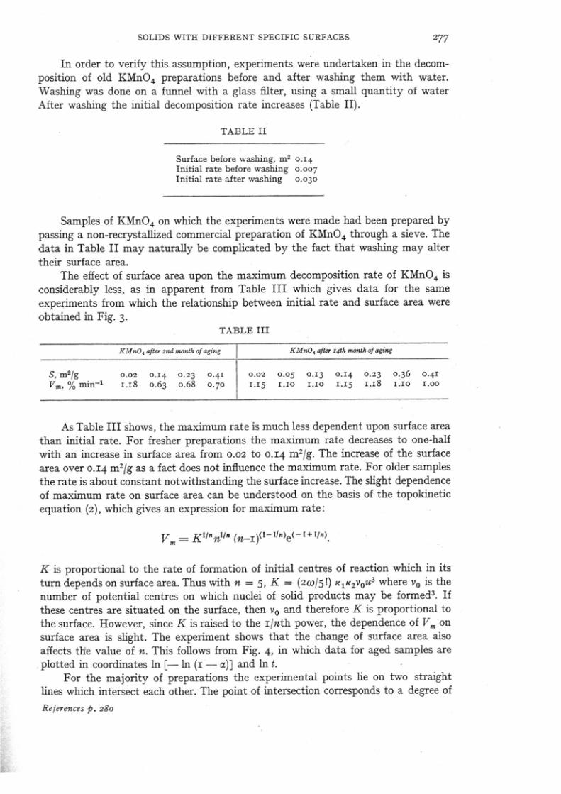
Kinetics by thermal analysis Reaction rates of processes involving solids with different specific surfaces B.V Yerofeyev Reactivity of solids 1961 Reaction kinetics by DTA H.E. Kissinger Anal Chem 1957 Analytical solution for Kissinger Equation P. Roura, J. Farjas J. Mater. Res. 2009 Data treatment in nonisothermal kinetics and diagnostic limits of phenomenological models N. Koga, J. Malek, J. Sestak, H. Tanaka Netsu Sukotei 1993 Forty years of Sestak-Berggren equation P. Simon Thermochim Acta 2011 Determination of activation energies by DTA G.O. Piloyan, I.D. Ryabchikov, O.S. Novikova Nature 1966 Diagnostic limits of phenomenological models of heterogeneous reactions and thermal analysis kinetics J. Šesták, J. Málek Solid State Ionics 1995

Reactivity of Solids, Proceedings of the 4th International Symposium (Amsterdam 1960): Amsterdam: Elsevier 1961 pp. 273-282

273

Analytical solution for the Kissinger equation

Pere Rouraa) and Jordi FarjasGrup de Recerca en Materials i Termodinamica (GRMT), Department of Physics,University of Girona, Campus Montilivi, E17071 Girona, Catalonia, Spain

(Received 25 March 2009; accepted 29 June 2009)

An analytical solution for the Kissinger equation relating the activation energy, E, withthe peak temperature of the reaction rate, Tm, has been found. It is accurate (relative errorbelow 2%) for a large range of E/RTm values (from 15 to above 60) that cover mostexperimental situations. The possibilities opened by this solution are outlined by applyingit to the analysis of some particular problems encountered in structural relaxation ofamorphous materials and in kinetic analysis.

I. INTRODUCTION

When the rate of a reaction is governed by a singlelimiting step, the evolution with time of the conversiondegree, a, is described by a differential equation of theform1:

dadt

¼ f ðaÞkðTÞ ; ð1Þ

where f(a) depends on the type of rate-controlling proc-ess and k(T) is the temperature-dependent rate constant.Usually, k(T) follows an Arrhenius dependence:

kðTÞ ¼ Ake�E=RT ; ð2Þ

where Ak is constant, E is the activation energy, T thetemperature, and R the gas constant. When the tempera-ture varies with time, Eq. (1) still holds for spatiallyhomogeneous reactions, whereas for heterogeneousreactions such as crystallization it is only approximate.2

The most common nonisothermal experiments involveconstant heating conditions, i.e.,

T ¼ T0 þ bt ; ð3Þwhere T0 is chosen low enough to have a negligibleeffect on the results. These kinds of experiments allowAk and E to be determined provided that a particularkinetics [f(a)] is assumed.

Despite the large number of kinetic models, there is asimple relationship between the kinetic parameters, Eand Ak, and the temperature, Tm, at which the transfor-mation rate is at its maximum. Namely,

E

RT2m

¼ A

be�E=RTm : ð4Þ

A is equal to Ak for most kinetics or is proportional toit.3 This equation was first derived by Kissinger.4 It is

widely used for the analysis of structural transformationsas diverse as the dehydrogenation of carbon nanotubes,5

the crystallization of glasses,6,7 and the thermal analysisof lipids, proteins, and biological membranes,8 becausethe slope of Ln(b/Tm

2) versus 1/RTm (Kissinger plot) isjust the activation energy. It is exact only for first-orderkinetics [f(a) = 1–a],9 and it is accurate for other kineticsprovided that E/RTm is large enough (for most kinetics,the error in E is lower than 2% if E/RTm > 10).9 A litera-ture review reveals that this does not represent a seriouslimitation to the applicability of Eq. (4): (i) E/RTm > 25for most glass-crystal transformations10 and (ii) we havefound values in the 8 to 35 range in reactions involvingpolymers11 and thermal decomposition of molecules5,12

(among them, values below 10 are scarce).Until now, the Kissinger Eq. (4) has mainly been used

for the analysis of experimental data through the popularKissinger plot. Using this equation to find the analyticalrelationship between the parameters involved in a givenreaction is not straightforward because the Kissingerequation itself lacks an exact analytical solution. In thiswork, we will show that within the range 15 < E/ RTm <60, which covers most experimental situations, an accu-rate analytical solution can be used. To illustrate theinterest in this solution, several applications are detailedat the end of this work. Most of them have proven usefulin a paper recently published by us.13 We should makeclear here that our analytical solution is not intended foruse instead of the Kissinger equation itself in the analy-sis of experimental data, where the use of the Kissingerplot is adequate. The examples at the end of the workindicate that its natural applications are in theoreticalanalyses.

II. THE ANALYTICAL SOLUTION

The Kissinger Eq. (4) can be rewritten in terms of thereduced activation energy, x � E=RT, and the reducedpre-exponential rate constant, ATm/b, as

a)Address all correspondence to this author.e-mail: pere.roura@udg.es

DOI: 10.1557/JMR.2009.0366

J. Mater. Res., Vol. 24, No. 10, Oct 2009 © 2009 Materials Research Society 3095

xm ¼ Ln

�ATmb

�þ Ln

�1

xm

�: ð5Þ

A plot of xm versus Ln(ATm/b) (inset of Fig. 1) revealsa quasilinear dependence with a slope close to 1 for theuseful xm range of most solid state reactions (i.e., 15 <xm < 60). This simple dependence arises because of thereduced variation of xm when ATm/b spans over manyorders of magnitude (see inset of Fig. 1). Consequently,an approximate analytical solution of Eq. (4) can bewritten as

xm ¼ LnATmb

1

xm0

� �; ð6Þ

where xm0 is a particular value between 15 and 60. Theaccuracy of this solution has been tested for severalvalues of xm0 and the relative error in the whole rangehas been plotted in Fig. 1. Relative errors below 2% areachieved with xm0 = 20. These are also the relative errorsof the activation energy, when Eq. (6) is solved for E:

E ¼ RTmLnATmb

1

xm0

� �; ð7Þ

and, when solved for Tm,

1

Tm¼ R

ELn

A

bE

R

1

x 2m0

� �; ð8Þ

the relative errors are twice those of E, because xm0 nowappears squared. Of course, the accuracy can be im-proved if the range of xm is restricted and xm0 is choseninside the range. The accuracy achieved for E is higherthan that obtained from most experiments. In addition, itis similar to the accuracy of the Kissinger equation itselfwhen applied to the analysis of non-first-order kinetics.9

Consequently, although Eqs. (6)–(8) are not exact, they

are accurate enough to be used in theoretical analysesinvolving the Kissinger equation. Some examples aregiven in Sec. III.

III. SOME APPLICATIONS

The first two examples concern structural relaxationprocesses in amorphous materials. These processes can-not be directly described by Eq. (1), because they are notgoverned by single activation energy. Consequently,analysis of the transformation temperature shift with theheating rate through the Kissinger equation can lead toerroneous interpretation of the activation energy.14

It is usually accepted that structural relaxation involvesa distribution of independent defects that relax to a lowerenergy state.15 A particular kind of defect is identifiedby its activation energy and many analyses consider thatthe pre-exponential rate constant is the same for alldefects.16,17 Therefore, structural relaxation can be formal-ly described by the superposition of a continuum of trans-formations characterized by a distribution of activationenergies, N(E). Any particular transformation will followEq. (1) and will obey the Kissinger equation.13 Underthese assumptions, a simple relationship can be foundbetween the peak temperature of a given transformationwithin the distribution and its activation energy. The de-rivative of Eq. (7) in Tm leads to

dTm ¼ dE=R

Ln ATmb

1xm0

� �þ 1

¼ BdE ; ð9Þ

where B is almost constant (almost independent of Tm)for a given heating rate. In other words, although forrelaxation experiments at a constant heating rate it ismore natural to describe the defects by the distributionof peak temperature; this distribution has a shape that isnearly identical to the distribution of activation energies.Additionally, B has a smooth dependence on the heatingrate. For the particular case of structural relaxation ofa-Si (take A � 1013 s�1, the Debye frequency),16 B in-creases by 20% when b increases from the usual valuesof conventional differential scanning calorimetry (1 K/s)to the high values of nanocalorimetry (104 K/s).18

Concerning the activation energy of the defects in thedistribution, we will show that, for constant A, it isalmost proportional to the peak temperature. Withoutany further approximation, application of Eq. (7) to(E1, Tm1) and (E, Tm) leads to:

E ¼ E1

Tm1

Tm 1þ 1

xm1

LnTmTm1

� �� �� E1

Tm1

Tm ; ð10Þ

where the last expression is obtained because xm1>>1.Of course, the higher xm1 the better the proportionalitybetween Tm and E. Thanks to this relationship, we haveshown in Ref. 13 that, when A is constant, the logarithmic

FIG. 1. Relative error in the activation energies delivered by the

analytical solution [Eq. (7)] with a single value of xm0 for the entire

range of interest of xm. Inset: exact solution of the Kissinger equation.

P. Roura et al.: Analytical solution for the Kissinger equation

J. Mater. Res., Vol. 24, No. 10, Oct 20093096

variations with time of selected properties during theisothermal relaxation of amorphous materials have aslope proportional to the annealing temperature.

The next two examples have a general interest inkinetic analysis. First of all, we will derive a relationshipthat allows calculating the shift of Tm when the heatingrate is increased from b1 to b2. From Eq. (8) we obtainthe exact formula (xm0 replaced by xmi):

Dð1=TmÞ � 1

Tm2

� 1

Tm1

¼ R

E½Lnðb1=b2Þ

þ 2Lnðxm1=xm2Þ� : ð11ÞSince, as commented previously, xm has a variation

smoother than that of b (in fact bR/AE), we can expandthe logarithm of xmi around xm1/xm2 = 1 (i.e., aroundTm2/Tm1 = 1). We obtain

Dð1=TmÞ ¼ R

ELnðb1=b2Þ � 2

Dð1=TmÞ1=Tm1

� �: ð12Þ

Solving for D(1/Tm) leads us to the desired result:

Dð1=TmÞ � 1

Tm1

Lnðb1=b2Þ2þ xm1

: ð13Þ

A similar, less accurate relationship was publishedseveral decades ago.19 Numerical analysis of our ap-proximate relationship reveals that, as expected, its ac-curacy improves when xm becomes higher. Considerthe particular case of a process with peak temperatureTm = 500 K and activation energy of 83.1 KJ/mol(xm = 20). When the heating rate is increased by afactor of 100, Eq. (13) predicts a shift of the peaktemperature of 132.4 K, which is very close to theexact result of 130.6 K.

Finally, we will consider second-order kinetics. Thisis the kinetics governing defect recombination in crys-talline materials. Their concentration, C, diminishesaccording to a bimolecular reaction:

dC

dt¼ �kCC

2 ; ð14Þ

where kC is thermally activated. With the definition ofthe transformed fraction as

a � C0 � C

C0

; ð15Þ

where C0 is the initial concentration, we arrive to theparticular form of Eq. (1) for a second-order reaction

dadt

¼ ðkCC0Þð1� aÞ2 ; ð16Þ

that, compared with Eqs. (1) and (2), leads to the conclu-sion that the reaction rate k(T) is proportional to C0. Thismeans, according to our analytical solution of theKissinger equation [Eq. (8)], the peak temperature will

depend on C0 through the pre-exponential constant A.When the initial concentration changes from C01 to C02,the shift of the peak temperature can be deduced, as wehave done for the previous application and we obtain

Dð1=TmÞ � 1

Tm1

LnðC02=C01Þ2þ xm1

: ð17Þ

This last formula has been applied in Ref. 13 to showthat in amorphous materials structural relaxation cannotbe described by a superposition of second-order recom-bination processes.

IV. CONCLUSIONS

To conclude, we can say that during the past 50 years,the Kissinger equation has been widely used for the anal-ysis of experiments concerning the kinetics of structuraltransformations. Despite this success, the particular func-tional dependencies on E and Tm make it difficult to usethe equation for general analytical predictions. Instead,predictions involve solving the equation numerically forparticular conditions. We hope that the analytical solu-tion obtained in this work will broaden the range ofapplications of the Kissinger equation.

ACKNOWLEDGMENT

This work was supported by the Spanish ProgramaNacional de Materiales under Contract No. MAT2006-11144.

REFERENCES

1. D.W. Henderson: Thermal-analysis of nonisothermal crystalliza-

tion kinetics in glass forming liquids. J. Non-Cryst. Solids 30, 301(1979).

2. J. Farjas and P. Roura: Modification of the Kolmogorov-Johnson-

Mehl-Avrami rate equation for non-isothermal experiments and

its analytical solution. Acta Mater. 54, 5573 (2006).

3. J. Farjas and P. Roura: Simple approximate analytical solution for

nonisothermal single-step transformations: Kinetic analysis.

AIChE J. 54, 2145 (2008).

4. H.E. Kissinger: Reaction kinetics in thermal analysis. Anal.Chem. 29, 1702 (1957).

5. J.W. Lee, H.S. Kim, J.Y. Lee, and J.K. Kang: Hydrogen storage

and desorption properties of Ni-dispersed carbon nanotubes.

Appl. Phys. Lett. 88, 143126 (2006).

6. E. Jona, P. Simon, K. Nemcekova, V. Pavlik, G. Rudinska, and

E. Rudinska: Thermal properties of oxide glasses. Part II. Activa-

tion energy as a criterion of thermal stability of Li2O�2SiO2�nTiO�2glass systems against crystallization. J. Therm. Anal. Calorim. 84,673 (2006).

7. A.P. Srivastava, D. Srivastava, and G.K. Dey: A study on micro-

structure, magnetic properties and kinetics of the nanocrystalliza-

tion of Fe40Ni38B18Mo4 metglass. J. Magn. Magn. Mater. 306,147 (2006).

8. B.D. Ladbrook and D. Chapman: Thermal analysis of lipids,

proteins and biological membranes. A review and summary of

some recent studies. Chem. Phys. Lipids 3, 304 (1969).

P. Roura et al.: Analytical solution for the Kissinger equation

J. Mater. Res., Vol. 24, No. 10, Oct 2009 3097

9. P. Budrugeac and E. Segal: Applicability of the Kissinger equation in

thermal analysis revisited. J. Therm. Anal. Calorim. 88, 703 (2007).10. H. Yinnon and D.R. Uhlmann: Applications of thermoanalytical

techniques to the study of crystallization kinetics in glass-forming

liquids. 1. Theory. J. Non-Cryst. Solids 54, 253 (1983).

11. S. Vyazovkin and N. Sbirrazzuoli: Isoconversional kinetic analy-

sis of thermally stimulated processes in polymers. Macromol.Rapid Commun. 27, 1515 (2006).

12. S.K. Padhi: Solid-state kinetics of thermal release of pyridine and

morphological study of [Ni(ampy)2(NO3)2]; ampy = 2-picolyla-

mine. Thermochim. Acta 448, 1 (2006).

13. P. Roura and J. Farjas: Structural relaxation kinetics for first and

second-order processes: Application to pure amorphous silicon.

Acta Mater. 57, 2098 (2009).

14. V.A. Khonik, K. Kitagawa, and H. Morii: On the determination

of the crystallization activation energy of metallic glasses. J.Appl. Phys. 87, 8440 (2000).

15. M.R.J. Gibbs, J.E. Evetts, and J.A. Leake: Activation-energy

spectra and relaxation in amorphous materials. J. Mater. Sci. 18,278 (1983).

16. J.H. Shin and H.A. Atwater: Activation-energy spectrum and

structural relaxation dynamics of amorphous-silicon. Phys. Rev.B 48, 5964 (1993).

17. W. Deceuninck, G. Knuyt, H. Stulens, L. Deschepper, and

L.M. Stals: Determination of the attempt frequency for relaxation

phenomena in amorphous metals. Mater. Sci. Eng., A 133, 337(1991).

18. J-F. Mercure, R. Karmouch, Y. Anahory, S. Roorda, and

F. Schiettekatte: Dependence of the structural relaxation of amor-

phous silicon on implantation temperature. Phys. Rev. B 71,134205 (2005).

19. C. Popescu and E. Segal: Variation of the maximum rate of

conversion and temperature with heating rate in non-isothermal

kinetics. 2. Thermochim. Acta 82, 387 (1984).

P. Roura et al.: Analytical solution for the Kissinger equation

J. Mater. Res., Vol. 24, No. 10, Oct 20093098

G

T

S

F

PI

a

ARRAA

KSSMM

drt

Taopt

isee

wo(ei

0d

ARTICLE IN PRESSModel

CA-75649; No. of Pages 2

Thermochimica Acta xxx (2011) xxx–xxx

Contents lists available at ScienceDirect

Thermochimica Acta

journa l homepage: www.e lsev ier .com/ locate / tca

hort communication

ourty years of the Sesták–Berggren equation

eter Simon ∗

nstitute of Physical Chemistry and Chemical Physics, Faculty of Chemical and Food Technology, Slovak University of Technology, Radlinského 9, SK-812 37, Bratislava, Slovak Republic

r t i c l e i n f o

rticle history:eceived 20 February 2011eceived in revised form 14 March 2011ccepted 23 March 2011

a b s t r a c t

The Sesták–Berggren equation, representing a powerful tool for the description of kinetic data by themodel-fitting methods, is analyzed. It is discussed that the exponents in the conversion function are non-integer in general and that the conversion function may not have a mechanistic interpretation. Within theframework of single-step approximation, the Sesták–Berggren equation enables to describe the kinetics

vailable online xxx

eywords:ˇesták–Berggren equationingle-step approximationodel-fitting methodechanistic interpretation

of complex condensed-state processes without a deeper insight into their mechanism.© 2011 Elsevier B.V. All rights reserved.

Kinetics of the processes in condensed phase is frequentlyescribed by the so-called general rate equation representing theeaction rate d˛/dt as a product of two mutually independent func-ions:

d˛

dt= k(T)f (˛) (1)

he temperature function, k(T), depends solely on temperature Tnd the conversion function, f(˛), depends only on the conversionf the process, ˛. The temperature function is prevailingly inter-reted as the rate constant and the conversion function is believedo reflect the mechanism of the process.

Fourty years ago, a paper by Sesták and Berggren [1] appearedn this journal introducing in Eq. (1) a three-parameter conver-ion function for a generalized description of reaction kinetics. Thequation is often named after their authors, i.e. the Sesták–Berggrenquation (habitually abbreviated as the SB equation):

d˛

dt= k(T)˛m(1 − ˛)n [−] (2)

here m, n, and p are the (generally non-integer) exponents. Latern, Gorbachev [2] demonstrated that, for isothermal conditions, Eq.2) can be transformed into three invariant expressions with twoxponents only. Among them, the following form is the one which

Please cite this article in press as: P. Simon, Fourty years of the Sesták–Bergg

s most frequently employed:

d˛

dt= k(T)˛a(1 − ˛)b (3)

∗ Tel.: +421 2 59325530; fax: +421 2 52926032.E-mail address: peter.simon@stuba.sk

040-6031/$ – see front matter © 2011 Elsevier B.V. All rights reserved.oi:10.1016/j.tca.2011.03.030

The exponents a and b in Eq. (3) may differ from those m and nintroduced in Eq. (2).

Eq. (3) can be encountered in the literature published before1971. Erofeev and Mitskevich in 1961 [3] pointed out that theexpansion and rearrangement of the differentiated form of theYerofeev equation lead to Eq. (3). As early as in 1940, Akulovreported Eq. (3) where the constants a and b called the “constants ofhomogeneity” [4]. Eq. (3) is also quite frequently cited in the liter-ature as an extended form of the Prout and Tompkins autocatalyticequation [5], for example in [6–9]. Nonetheless, Eq. (3) is generallyconsidered a transformation of Eq. (2) so that it is equally called theSB equation.

Eq. (3) is widely applied to the study of not only isothermal,but also non-isothermal processes; mathematical correctness ofeither description was justified in [10]. Later it was shown [11]that this two-parameter model retains its physical meaning onlyfor a ≤ 1. Málek pointed out that the classical nucleation-growthequation (often abbreviated as JMAYK) is actually a special case ofthis two-parameter SB model and thus SB equation represents aplausible alternative description for the crystallization processestaking place in non-crystalline solids [12]. The increasing value ofthe exponent a indicates a more important role of the precipitatedphase on the overall kinetics. It also appears that a higher valueof the second exponent (b > 1) indicates increasing reaction com-plexity; however, the temptation to relate the values of a and b toa reaction mechanism can be doubtful and should be avoided [12]without complementary measurements [13,14].

ren equation Thermochim. Acta (2011), doi:10.1016/j.tca.2011.03.030

Due to its ability to describe variety of kinetic data both oforganic and inorganic origin [9], the SB equation attracts muchattention. It was believed that it can be considered a univer-sal expression for kinetic models [15]. For certain combinations

ING

T

2 ica Ac

oicmseof

t[rombtifndtsrnotc

ttasarkopa

dt1cpei

[

[

[

[

[

[

[

[

[

[

ARTICLEModel

CA-75649; No. of Pages 2

P. Simon / Thermochim

f exponents, the conversion function in SB equation can mergen most conversion functions representing mechanisms of pro-esses. For further improvement of the mechanistic interpretation,ultiplying the SB equation by an accommodation constant was

uggested [16]. Nevertheless, it was recognized that kinetic mod-ls of solid-state reactions are often based on a formal descriptionf geometrically well-defined bodies under isothermal conditions;or real processes, these assumptions are evidently incorrect [17].

In contrast with the mechanistic interpretations of Eq. (1) men-ioned above, there is the idea of the single-step approximation18,19]. The history and contradictions of the concept of single-stepeaction have been discussed in [20]. The approximation is basedn the fact that the processes in condensed phase tend to occur inultiple steps that have different rates. Each reaction step should

e described by its own kinetic equation. It has been demonstratedhat, neither for the simplest cases, the kinetic equations character-zing complex mechanisms cannot be reduced into the factorizedorm of Eq. (1) [21]. Hence, it has been concluded that Eq. (1) isot a true kinetic equation; it is just a mathematical tool for theescription of kinetic data [18,19,21]. The single-step approxima-ion resides in replacing the set of differential rate equations by theingle-step generalized rate equation. The functions k(T) and f(˛)epresent, in general, just the temperature and conversion compo-ents of the kinetic hypersurface; this hypersurface is a dependencef conversion as a function of time and temperature [18]. Thus,he temperature function may not be the rate constant and theonversion function may not reflect the reaction mechanism.

The value and wide applicability of the SB equation surpasses inhe light of the single-step approximation. The conversion func-ions in Eqs. (2) or (3) are able to describe both the S-shapedccelerating kinetic curves and the n-th order ones. Due to the pos-ibility of adjustment of the exponents, the function is very versatilend flexible. In general, the values of exponents may not reflect theeaction mechanism; on the other hand, they enable to describeinetic data and modeling the kinetics of the overall process with-ut a deeper insight into its mechanism. The SB equation providesurely formal description of the kinetics and it should be appliednd understood in this way.

The Sesták–Berggren equation represents a powerful tool for theescription of kinetic data by the model-fitting methods. Accordingo SCOPUS, the paper [1] was cited 316 times since 1996. Since971, the paper was cited nearly 600 times and probably is the most

Please cite this article in press as: P. Simon, Fourty years of the Sesták–Bergg

ited paper in the history of almost twenty two thousand papersublished in Thermochimica Acta. There are no doubts that the SBquation will continue being widely applied also in future, eithern the form of Eq. (2) or Eq. (3).

[

[

PRESSta xxx (2011) xxx–xxx

Acknowledgements

The author would like to express his cordial thanks to Dr. S. Vya-zovkin for invaluable comments and for providing the old Russianliterature sources.

The financial support from the Slovak Scientific Grant Agency,grant No. VEGA 1/0660/09, is gratefully acknowledged.

References

[1] J. Sesták, G. Berggren, Study of the kinetics of the mechanism of solid-state reactions at increasing temperature, Thermochim. Acta 3 (1971) 1–12.

[2] V.M. Gorbachev, Some aspects of Sesták’s generalized kinetic equation in ther-mal analysis, J. Therm. Anal. 18 (1980) 193–197.

[3] D.A. Young, Decomposition of Solids, Pergamon Press, Oxford, 1966, p. 35.[4] E.A. Prodan, Inorganic Topochemistry, Nauka i Technika, Minsk, 1986, p.153 (in

Russian).[5] E.G. Prout, F.C. Tompkins, The thermal decomposition of potassium perman-

ganate, Trans. Faraday Soc. 40 (1944) 488–498.[6] J. Sesták, Review of kinetic data evaluation from nonisothermal and isothermal

TG data, Silikáty 11 (1967) 153 (in Czech).[7] W.L. Ng, Thermal decomposition in the solid state, Aust. J. Chem. 28 (1975)

1169–1178.[8] J. Malek, T. Mitsuhashi, J.M. Criado, Kinetic analysis of solid-state processes, J.

Mater. Res. 16 (2001) 1862–1871.[9] A.K. Burnham, Application of the Sesták–Berggren equation to organic and

inorganic materials of practical interest, J. Therm. Anal. Calorim. 60 (2000)895–908.

10] T. Kemény, J. Sesták, Comparison of crystallization kinetics determinedby isothermal and non-isothermal methods, Thermochim. Acta 110 (1987)113–129.

11] J. Málek, J.M. Criado, J. Sesták, J. Militky, The boundary conditions for kineticmodels, Thermochim. Acta 153 (1989) 429–432.

12] J. Málek, Kinetic analysis of crystallization processes in amorphous materials,Thermochim. Acta 355 (2000) 239–253.

13] J. Sesták, Thermophysical Properties of Solids: A Theoretical Thermal Analysis,Elsevier, Amsterdam, 1984.

14] J. Sesták, Science of heat and thermophysical studies: a generalized approachto thermal analysis, Elsevier, Amsterdam 2005.

15] J. Málek, J.M. Criado, Is the Sesták–Berggren equation a general expression ofkinetic models? Thermochim. Acta 175 (1991) 305–309.

16] L.A. Pérez-Maqueda, J.M. Criado, P.E. Sánchez-Jiménez, Advantages of com-bined kinetic analysis of experimental data obtained under any heating profile,J. Phys. Chem. A110 (2006) 12456–12462.

17] N. Koga, J. Malek, J. Sestak, H. Tanaka, Data treatment in non-isothermal kineticsand diagnostic limits of phenomenological models, Netsu Sokutei 20 (1993)210–223.

18] P. Simon, Single-step kinetics approximation employing non-Arrhenius tem-perature functions, J. Therm. Anal. Calorim. 79 (2005) 703–708.

19] P. Simon, Considerations on the single-step kinetics approximation, J. Therm.Anal. Calorim. 82 (2005) 651–657.

ren equation Thermochim. Acta (2011), doi:10.1016/j.tca.2011.03.030

20] S. Vyazovkin, Kinetic concepts of thermally stimulated reactions in solids:a view from a historical perspective, Int. Rev. Phys. Chem. 19 (2000) 45–60.

21] P. Simon, The single-step approximation: attributes, strong and weak sides, J.Therm. Anal. Calorim. 88 (2007) 709–715.

Solid State lonics 63-65 (1993) 245-254 North-Holland

SOLID STATE IONICS

Diagnostic limits of phenomenological models of heterogeneous reactions and thermal analysis kinetics

Jaroslav ~est~ik Division of Solid State Physics, Institute of Physics of the Academy of Sciences of the Czech Republic, Cukrovarnickd 10, 162 O0 Prague, Czech Republic

and

J i l l M~tlek Joint Laboratory of Solid State Chemistry of the Academy of Sciences of the Czech Republic, and University of Chemical Technology, ~s. Legil sq. 565, 532 I0 Pardubice. Czech Republic

Kinetic models of solid-state reactions are often based on a formal description of geometrically well defined bodies treated under strictly isothermal conditions; for real processes these prepositions are evidently incorrect. It can be equally useful to find an empirical function containing the smallest possible number of constants. In such a case the models of heterogeneous kinetics can be assumed as a distorted (fractal) case of the simpler homogeneous kinetics and mathematically treated by multiplying by an "accommodation" function. In addition, the conventional thermoanalytical (TA) studies apply intentionally the experimental conditions with constant heating and/or cooling where the model's validity must again be investigated. The general method of kinetic data evaluation is proposed to include two-step evaluation: first, determining the activation energy, E, from a set of TA curves at different heating rates, and second, using the pre-established E to search for the reaction mechanism by analyzing the entire course of the single TA curve. In this respect the possibility of a simultaneous determination of all kinetic data is discussed. The computer method is recommended to be based on the evaluation of two specific functions available for a direct derivation from experimental data.

1. Introduction

In contradict ion to the well established spot mea- surements frequently employed to investigate solid- state reactions, although affected by inadequate freeze-in and poor localization of the reaction, the centered measurements of a properly representing the average state of a sample are often considered less convenient due to the superstitiously bad rep- utat ion of its mere phenomenological character. The latter group is represented by methods of thermal analysis (TA) carried out under constant heating a n d / o r cooling often treated in terms of a homoge- neous-like kinetic description yielding fractal values of reaction orders assumed to have meaningless sense in heterogeneous kinetics. However, even the ho- mogeneous reactions exhibiting non-randomness of the reactant distr ibution a n d / o r diffusion-controlled

subprocess can be described by reactions on fractal domains, the hallmark being the anomalous reaction orders. It is clear that the present state of the art of the thermal analysis kinetics [ 1 ] as applied to het- erogeneous reactions is not appropriate to the so- phisticated means available in solid-state chemistry, the linkage of most treatments to the tradit ional geo- metrical description being very firm and hard to overcome [1-3] . The use of phenomenological models has been criticized [2] but a unified ap- proach is still missing as well as a correlation be- tween the microscopic process (detectable only lo- cally under not well guaranteed condit ions) and the macroscopic process (capable of measuring in situ even at changing temperatures) . Our philosophy is to show that we can merely distinguish proportion- able relevancy of the individual groups of phenom- enological models to match with the gradual increase

0167-2738/93/$ 06.00 © 1993 Elsevier Science Publishers B.V. All rights reserved.

246 .L ~est~k, J. MMek / Phenomenological models of heterogeneous reactions

of complexity of an experimentally determined ki- netic curve from TA measurements of the reaction investigated.

Extraction of the maximum relevant information from non-isothermal data obtained by such (TA) techniques and a consequent kinetic process mod- eling are typical tasks of data treatment [1]. The problem of the validity and applicability of mathe- matical models in kinetic analysis of TA data is still considered a very controversial topic [ 2 ]. Apart from the question of the physical meaning of kinetic pa- rameters (which has not been answered until now) there are several problems inherent in the mathe- matical formalism used for the description of kinetic processes [3 ]. The aim of this paper is to discuss the possibilities and limitations of kinetic analysis of non- isothermal data.

In the following section we first briefly review the mathematical relationship used to describe TA data. A subsequent section presents some consequences of the mutual correlation o f kinetic parameters and their implications for a reliable kinetic analysis. Finally, a completely new way of kinetic analysis is outlined so as to eliminate the effect o f experimental condi- tions. The method allows the determination of the most suitable kinetic model and calculation o f a complete set of kinetic parameters.

function f ( a ) represents a mathematical expression of the kinetic model.

There are several kinetic models derived from the geometry of the reaction interface [3]. The mathe- matical formulae of the most frequently cited models are summarized in table 1. These kinetic model functions derived on the basis of physical-geomet- rical assumptions of regularly shaped bodies evi- dently can hardly describe real heterogeneous sys- tems where we have to consider, for instance, irregular shapes of reacting bodies, polydispersity, shielding and overlapping effects of phases involved in the process, etc.; see fig. 1. From this point of view it would be useful to find an empi r i ca l f ( a ) function containing the smallest possible number of con- stants, so that it is flexible enough to describe real TA data as closely as possible [ 3 ]. Later this concept led to an idea that such an empirical kinetic model would provide a general expression for all kinetic equations shown in table 1.

Unfortunately, these two aspects are very often confused. So we believe it will be useful to discuss these problems, which influence the applicability of the empirical kinetic models in thermal analysis.

3. The empirical kinetic models

2. The kinetic equation

Most reactions studied by TA techniques can be described by an equation:

d a / d t = A e - X f ( a ) , ( 1 )

where x = E / R T is the reduced activation energy. The

Twenty years ago, Sestfik and Berggren [4] pro- posed an empirical kinetic model in the form

f ( a ) = a m ( 1 - - a ) ~ - - l n ( 1 - - o l ) ] ~ (2)

It was believed [2,3] that this kinetic equation, con- taining as many as three exponential terms, is ca- pable of describing any TA curve. Further mathe- matical analysis [ 5 ] of eq. (2) has shown, however, that no more than two kinetic exponents are nec-

Table 1 The kinetic models.

Model Symbol f( a )

Johnson-Mehl-Avrami A. 2D reaction R2 3D reaction R3 2D diffusion D2 Jander equation 9 3 Ginstling-Brounshtein Da

n( l -o l ) [ - ln(1-e~)] l - ' / " ( 1 - a ) '/2 ( l - - a ) 1/3

l / [ - l n ( 1 - a ) l ( l - c~)2/3/[ t - ( 1 -c~) 2/3]

3 [(1--O:)-L/3-- l ]

J. ,~estdk, J. Mdlek / Phenomenological models of heterogeneous reactions 247

Horn

oe 0 • 0 • 0 0

• o .o0 L, o . j Nucl

Her I D

2D

3D

Reol

Fig. 1. Schematic diagram of a hypothetical transfer of the sys- tem geometry from a non-dimensional homogeneous-like model (obeying reaction order model f(ot ) = ( l - o~ )", upper left ) to the idealized heterogeneous model by introduction od dimensional- ity, due to the interface formation (nucleation obeying the loga- rithmic model f(oQ = ( 1 - a ) [In( 1 - a ) ]m, lower left) and in- terface growth (controlled by either the linear law of a chemical reaction or parabolic law of diffusion, second column, compare table 1, R and D models). It is important to recall that the char- acter of the kinetic description changes drastically from the con- centration-dependent (HOM) to that of the interface-to-volume dependent (HET). The last column illustrates the behavior of real particles which does require to account for polydispersity, shielding and overlapping, unequal mixing and/or non-regular shapes and anisotropy (third column from top). Its kinetic mod- eling is mathematically difficult and can be formally accom- plished by the introduction of an accomodation function, h (a), to multiply the basic monomolecular law ( l - a ) , i.e. f(a)=(1-oQh(a), where h(a) can take the form of either function, ( 1 - a ) i - n, [ _ In ( 1 - ct ) ] " and/or a p. It helps partic- ularly to fit the prolonged reaction tails due to the actual behav- ior of real particles and can match the particle non-sphericity in the view of morphology description in terms of characteristic di- mensions (usually the longest particle length), interface (aver- age boundary line ) and volume (mean section area), see bottom left. For the sake of illustration, the original and reacted parts are distinguished by hatching.

essary. Therefore after e l imina t ing the th i rd expo- nen t ia l t e rm in eq. (2 ) the f inal form ob t a ined is

f ( c t ) = o t t o ( 1 - a ) " . (3 )

In the l i terature the equa t ion (3) is cited as the Ses- t f ik-Berggren (SB) kinet ic model . The exponents m and n have the signif icance of the kinet ic parameters of the process. I f the exponen t m is set equal to zero, the r em a in ing exponen t n is then called the react ion order ( R O ) . This approach is of ten used for a gen- eral descr ip t ion of all he terogeneous processes, al- though it has on ly l imi ted appl icabi l i ty [6] .

Both the SB and RO models can also be under - s tood in te rms of the accomoda t ion func t ion in t ro- duced by Sest~ik [ 7]. In this case the he terogeneous kinet ics is a s sumed as a d is tor ted case of the s impler homogeneous kinetics. The accomoda t ion func t ion then expresses the dev ia t ion of the more complex re- act ion m e c h a n i s m from the ideal case; see fig. 1.

Recent ly we have shown [8] that the SB model canno t be cons idered as a general expression of the kinet ic models ( table 1 ) for the true (or fixed va lue) ac t iva t ion energy, E. Nevertheless , this is no t so ev- iden t for any arbi t rar i ly chosen value of the act iva- t ion energy which is called here the appa ren t acti- va t ion energy, Eapp [2] . The val id i ty of these procedures and the resul t ing func t ions when deriv- ing the kinet ic mode ls in ques t ion was approved also for non- i so the rma l cond i t ions elsewhere [ 9,10 ].

3.1. The reaction order model

Criado et al. [ 11 ] have shown that any TA curve can be descr ibed by the R O model ins tead o f the true one for a cer ta in va lue of the apparen t ac t iva t ion en- ergy. Recent ly it was found [ 12 ] that the rat io of the apparen t and true ac t iva t ion energies (Eapp/E) can be expressed for the apparen t RO model by the fol- lowing equa t ion :

E a p p _ f ( a p ) napp (4) E f ' ( a p ) l - a p '

where c% is the degree o f convers ion at the maxi- m u m of the TA peak and napp is an apparen t kinet ic exponen t of the RO model . The value o f n,pv is char- acterist ic for the true kinet ic mode l bu t ap depends also on the xp ( reduced ac t iva t ion energy at the max- i m u m of the TA peak) . Therefore the value of E~pp/

248 J. Sestdtk, J. Mddek / P h e n o m e n o l o g i c a l m o d e l s o f he t e rogeneous react ions

E increases slightly with increasing Xp for diffusion models (i.e. D2, D3 and D4). On the other hand, the ratio EapJE decreases with increasing Xp for the A, model as corresponds to the following equation [ 13 ]:

Eap p -- n - 1 + 1 , (5) E xo~(Xp)

where n is the true kinetic exponent of the A, model and 7r(x) is the approximation of the temperature integral in the form [ 14 ]

x 3 + 18x z + 8 8 x + 9 6 ~ ( x ) = X 4 + 20x3_t_ 1 2 0 x Z + 2 4 0 X + 120 " (6)

It is noteworthy that the empirical relationship E a p p /

E=1 .05 E - 0 . 0 5 found by Criado et al. [11] cor- responds to the general equation (5) for Xp= 38.3.

The limiting values o f the parameters nap p and E~pp/E are summarized in table 2 for the kinetic models discussed.

3.2. The Sestdtk-Berggren model

The ratio of the apparent and true activation ener- gies can be expressed for the SB model in the fol- lowing form [ 12 ]:

EaPp- f ( a P ) ( r/app - mape'] (7) E f ' ( a p ) 1 - a p ap }"

By rewriting eq. ( 1 ) for an apparent activation en- ergy we obtain:

Yapp ( a ) = (dot /dt) exp (Eapp/R T). ( 8 )

The function yapp(a) defined by eq. (8) is propor- tional to function f ( a ) that represents the apparent kinetic model of the process. Therefore, by plotting the Yapp ( a ) dependence, the apparent kinetic model can be determined.

The function Y~vv(a) has a maximum at aM for the SB model. It can be shown #J that the maximum

Table 2 The values of apparent parameters (Xv~OO) for the RO model.

True model napp E,,pr,/ E

An 1 n D2 0.269 0.483 D3 0.666 0.5 D 4 0.420 0.495

is confined to the interval 0 < o~ M < OLp and it can be used to determine the apparent kinetic exponent ra- tio [13]

m a p p _ a M (9) nap p I -- OL M

It should be stressed that any change of the value of the apparent activation energy leads to a different value of the ratio mapp/n,pp. Therefore both appar- ent kinetic exponents are mutually interdependent. A characteristics napp versus mapp dependence can be found for each true kinetic model. These plots (full lines) calculated using eqs. (7) and (9) are shown in fig. 2. The dashed lines correspond to the different values of the maxima of the function yapp((~). An important feature of the napp-mapp plot is that it is characteristic for the true kinetic model. Neverthe- less, it can be seen that these plots are identical for the D3 and R3 models. There is also one common curve corresponding to the An model regardless of the values of the true kinetic exponent, n. Similar be- havior was observed also for other types of reference plots [ 15,16 ]" see fig. 2.

Many works are concerned with the kinetic anal- ysis of a single TA curve. However, these methods are somewhat problematic because of the apparent kinetic models. For example, the popular Freeman

*~ It is evident that if the kinetic exponent, m, is equal to zero (i.e. for the RO model) , then aM=0. On the other hand Eapp should not be negative. Therefore it follows from eq. ( 7 ) that o< M has to be lower than a w

o .

.LVA(*O

D3,/L1

R2 D,~_

DI

i~: l l r ' : l r iT~ ' r ' l ) , , r [ ) ' l r , , ;~, , , , , : : , !

tit :

Fig. 2. Apparent kinetic exponents of the SB (mapp, napp) corre- sponding to the DE, D3, D4, R2, R3 and J M A ( n ) kinetic models.

J. ~estdk, .L Mdlek / Phenomenological models of heterogeneous reactions 249

and Carroll method [ 17] was derived for the RO model. Therefore, this method always gives apparent parameters napp and Eap p corresponding to the RO model regardless of the true kinetic model. Similarly, it must be borne in mind that the non-linear or mul- tiple linear regression methods can lead to incorrect results because any TA curve can be interpreted within the scope of several apparent kinetic models (RO or SB) depending on the value of the apparent activation energy.

On the other hand, if the true activation energy is known, the SB kinetic model can be found very use- ful in real heterogeneous systems [6,18,19], where other kinetic models cannot be successfully used for a quantitative description of the experimental data.

4. Correlation of the kinetic parameters

Both the activation energy and the pre-exponen- tial factor in eq. (1) are mutually correlated [20]. This correlation can be expressed by the following equation (see Appendix):

l n A = a + b E , (10)

where a and b are constants. Any change in the ac- tivation energy is, therefore, "compensated" by the change of In A as expressed by eq. (10). From this point of view, it seems that the methods of kinetic analysis aiming to ascertain all kinetic parameters from only one experimental TA curve are somewhat problematic. Similarly, as in the preceeding Section, we have to realize that this problem cannot be solved even using the most sophisticated non-linear regres- sion algorithms unless the kinetic models or at least one kinetic parameter is a priori known.

The value of E can further consist of the elemen- tary parts arising from the partial reaction steps [21 ], i.e. nucleation, interface chemical reaction and di- fussion, which became particularly important in the analysis of glass crystallization [22,23 ].

mental TA curve. This problem can be solved, how- ever, if the true activation energy is known. Then the most probable kinetic model can be determined and subsequently the pre-exponential term is calculated. The method of kinetic analysis is described in the following sections.

5.1. Calculations of the activation energy

The calculation of the activation energy is based on multiple scan methods where several measure- ments at different heating rates are needed. Probably the most popular in this family is the Kissinger method [25] based on the equation derived from the condition for the maximum rate on a TA curve. A very similar method of calculation of activation energy is the Ozawa method [ 26 ].

An alternative method of calculation of the acti- vation energy is the Isoconversional method which follows from the logarithmized form of the kinetic equation ( 1 ):

In (dc~/dt)= ln{Af( t~)}-E/RT. (11)

The slope ofln (dc~/dt) versus 1 /Tfor the same value of a gives the value of the activation energy. This procedure can be repeated for various values of ct. So it easily allows one to check the invariance of E with respect to c~, which is one of the basic assump- tions in kinetic analysis. Hence, the isoconversional method can be recommended for the calculation of the E.

On the other hand, we cannot recommend the Freeman-Carroll method [17] because it was de- rived for the RO (n) model and, therefore, due to the mutual correlation of kinetic parameters, this method always gives apparent kinetic parameters nap p and Eap p corresponding to the RO (napp), regardless of the true kinetic model.

5.2. Determination of the kinetic model

5. The kinetic analysis

The correlation of kinetic parameters and the ap- parent kinetic models does not allow us to perform correctly the kinetic analysis using only one experi-

Once the activation energy has been determined it is possible to find the kinetic model which best de- scribes the measured set of TA data. It can be shown that for this purpose it is useful to define two special functions y(c~) and z(o~) which can easily be ob- tained by simple transformation of the experimental

250 J. ,~estdk, J. Mdlek /Phenomenological models of heterogeneous reactions

data. These functions can be formulated as follows [27,28]:

y (a ) = (da/dt )e x , (12)

z (a ) = n ( x ) (da /d t )T / f l . (13)

The function y (a ) is proportional to the function riot). Thus by plotting the y (a ) dependence, nor- malized within the interval (0, 1 ), the shape of the function f ( a ) is obtained. The function y ( a ) is, therefore, characteristic for a given kinetic model, as shown in fig. 3, and it can be used as a diagnostic tool for kinetic model determination. The mathe- matical properties of the y ( a ) function for basic ki- netic models are summarized in table 3. The func- tion y (a ) has a maximum aM ~ (0, ap) both for the HMA (n > 1 ) and SB (m, n) model (see Appendix eqs. (A.13) and (A.14)).

It should be stressed that the shape of function y ( a ) is strongly affected by E. Hence the true ac-

JMA(3)

0.o°°, ......

c(

Fig. 3. Typical shapes of function y(a) for several kinet ic models.

Table 3 Proper t ies of the funct ion y ( a ) for basic k ine t ic models

Model y ( a )

J M A ( n )

R2

R3 D2 D3 D4

concave, for n < 1 linear, for n = 1 m a x i m u m , for n > 1 convex

convex concave concave concave

tivation energy is decisive for a reliable determina- tion of the kinetic model because of the correlation of kinetic parameters.

Similarly we can discuss the mathematical prop- erties of the function z (a) . It is fairly easy to de- monstrate (see Appendix, eq. A.10)) that the func- tion z ( a ) has a maximum at 0% for all kinetic models summarized in tables 1 and 2. This param- eter has characteristic values [ 13 ] for basic kinetic models as summarized in table 4. It is interesting that the a~ ° practically does not depend on the value of the activation energy used to calculate the function z ( a ) (in fact it varies within 1% of the theoretical value). An important fact is that a~ is invariant with respect to the kinetic exponent for the JMA(n) model. On the other hand, for both the RO(n) and SB (m, n) models, the parameter a ~ depends on the values of the kinetic exponents as shown in fig. 4.

It is evident that the shape of the function y (a ) as well as the maximum, a~ , of the function z ( a ) can be used to guide the choice of a kinetic model. Both parameters aM and a ~ are especially useful in this respect. Their combination allows the determi- nation of the most suitable kinetic model, as shown by the scheme in fig. 5. As we can see, the empirical SB (m, n) model gives the best description of TA data i f a ~ ~0.632 and aM ~ (0, ap). According to our ex- perience, these conditions are fulfilled for some solid- state processes [29,30].

0.8

0.7

0.6

0.5

0,4

0.3 0.3

~-~ SB(0.8, n)

0.8 1.3 1 8 2.3 2.8 3 3 3 8

T I

Fig. 4. The dependence of the m a x i m u m of the funct ion z ( a ) , a ~ , on the kinet ic exponent , n, for the R O ( n ) and SB(m, n)

k ine t ic models .

J. ~est6k, J. MMek / Phenomenological models of heterogeneous reactions 251

_-_9

,j

~M = 0

0 < aM<

c°nvexl

-- [concavo 1

---~ linear

> RO(n<l)

D2

D3

> D4

RO(n>l)

JMA(n<I)

> JMA(1)

) JMA(n>I)

> SB(m,n)

~p = 0.834

a p = 0 . 7 0 4

~p = 0.776

~p = 0. 632 (

Fig. 5. Schematic diagram of the kinetic model determination.

7:q

5.3. Calculation of kinetic exponents

Once the kinetic model has been determined, the kinetic exponents n (or m) can be calculated for the RO (n), JMA (n) or SB (m, n ) model. The calcula- tion method depends on the kinetic model and is de- scribed below.

5.3.1. RO(n) model The kinetic exponent n ~ 0 for this model can be

calculated iteratively using the equation:

( 1 - n ) ' / ' " - ' ) a p = l - 1+ xvn(Xp) (14)

n

This equation is obtained from eq. (A.4). We point out that it was derived originally by Gorbachev [ 5 ] for a simplified approximation: ~z (xp) = 1 / (xp + 2 ).

5.3.2. JMA(n) model If the function y / a has a maximum at aM e (0, ap),

i.e. for n> 1, then the kinetic exponent, n, is calcu- lated using eq. (A. 13) rewritten in a somewhat dif- ferent form:

1 n= l + l n ( 1 - - a M ) " (15)

If the function y(a) decreases steadily (i.e. n~< 1 ), then the parameter, n, can be calculated by the ~a- tava method [ 31 ]

In[ - I n ( 1 - a ) ] =cons t -nE /RT , (16)

i.e. from the slope of the plot ofln( - I n ( 1 -o~) ) ver- sus 1 /T. An alternative method of calculation is based on the following equation (obtained from eq. (A.4)):

1 -xpzt(Xp) n= (17)

l n ( 1 - a p ) + 1

It is known that the ~atava method [ 31 ] gives slightly higher values of the parameter n. On the other hand, eq. (1) gives lower ones. From our experience it seems that an average of these two values is a good approximation of the kinetic exponent.

5.3.3. SB(m, n) model The kinetic parameter ratio, p = m/n, is calculated

using eq. (A. 14) rewritten as follows:

p=OtM/ ( l--OtM) . (18)

Eq. ( 1 ) can be rewritten in the form:

l n [ (da /d t ) eX]+lnA+nln[aP(1 -a ) ] . (19)

The kinetic parameter, n, corresponds to the slope of linear dependence In [ ( d a / d t ) e x] versus l n [ a P ( 1 - a ) ] for a e (0.2, 0.8). Then the second kinetic exponent is m=pn.

252 J. Sest(tk, J. M(dek /Phenomenological models of heterogeneous reactions

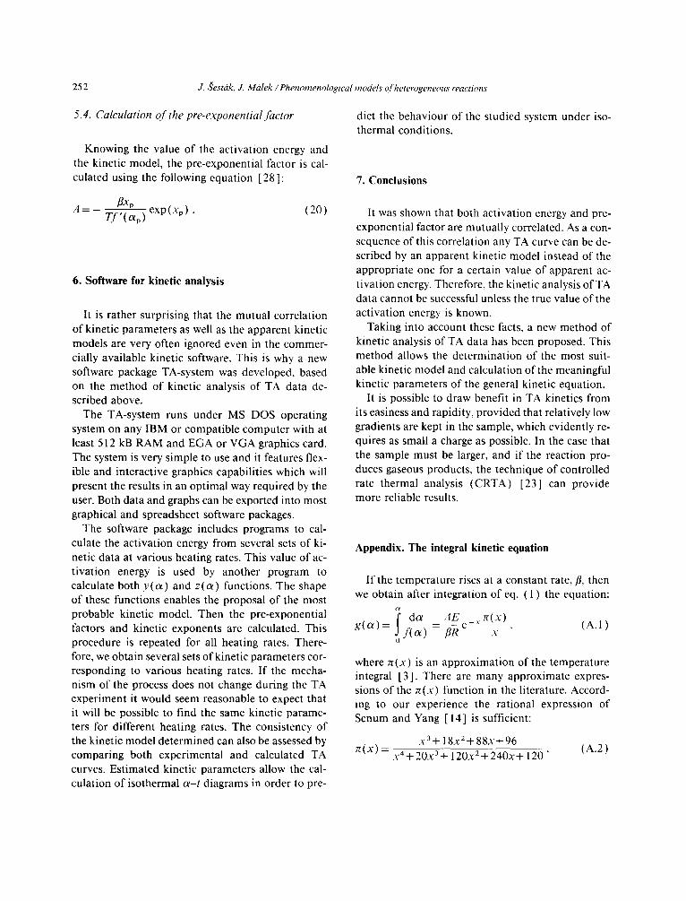
5.4. Calculation of the pre-exponential factor

Knowing the value of the activation energy and the kinetic model, the pre-exponential factor is cal- culated using the following equation [28]:

•Xp A = T f ' ( ~ p ) exp(xp) . (20)

6. Software for kinetic analysis

It is rather surprising that the mutual correlation of kinetic parameters as well as the apparent kinetic models are very often ignored even in the commer- cially available kinetic software. This is why a new software package TA-system was developed, based on the method of kinetic analysis of TA data de- scribed above.

The TA-system runs under MS DOS operating system on any IBM or compatible computer with at least 512 kB RAM and EGA or VGA graphics card. The system is very simple to use and it features flex- ible and interactive graphics capabilities which will present the results in an optimal way required by the user. Both data and graphs can be exported into most graphical and spreadsheet software packages.

The software package includes programs to cal- culate the activation energy from several sets of ki- netic data at various heating rates. This value of ac- tivation energy is used by another program to calculate both y(c~) and z(c~) functions, The shape of these functions enables the proposal of the most probable kinetic model. Then the pre-exponential factors and kinetic exponents are calculated. This procedure is repeated for all heating rates. There- fore, we obtain several sets of kinetic parameters cor- responding to various heating rates. I f the mecha- nism of the process does not change during the TA experiment it would seem reasonable to expect that it will be possible to find the same kinetic parame- ters for different heating rates. The consistency of the kinetic model determined can also be assessed by comparing both experimental and calculated TA curves• Estimated kinetic parameters allow the cal- culation of isothermal c~-t diagrams in order to pre-

dict the behaviour of the studied system under iso- thermal conditions.

7. Conclusions

It was shown that both activation energy and pre- exponential factor are mutually correlated. As a con- sequence of this correlation any TA curve can be de- scribed by an apparent kinetic model instead of the appropriate one for a certain value of apparent ac- tivation energy. Therefore, the kinetic analysis o f TA data cannot be successful unless the true value o f the activation energy is known.

Taking into account these facts, a new method of kinetic analysis of TA data has been proposed. This method allows the determination of the most suit- able kinetic model and calculation of the meaningful kinetic parameters of the general kinetic equation.

It is possible to draw benefit in TA kinetics from its easiness and rapidity, provided that relatively low gradients are kept in the sample, which evidently re- quires as small a charge as possible. In the case that the sample must be larger, and if the reaction pro- duces gaseous products, the technique of controlled rate thermal analysis (CRTA) [23] can provide more reliable results.

Appendix. The integral kinetic equation

If the temperature rises at a constant rate, fl, then we obtain after integration of eq. ( 1 ) the equation:

f da AE ~(x) g ( a ) = f ~ - ) _ ~-~ e - x - ( A . l )

• X 0

where g(x) is an approximation of the temperature integral [3]. There are many approximate expres- sions of the ~z(x) function in the literature. Accord- ing to our experience the rational expression of Senum and Yang [ 14 ] is sufficient:

x3+ 18xZ+88x+96 g ( x ) = x a + 2 0 x 3 + 120x2+240x + 120 " (A.2)

J. ~estdk, J. Mdlek /Phenomenological models of heterogeneous reactions 253

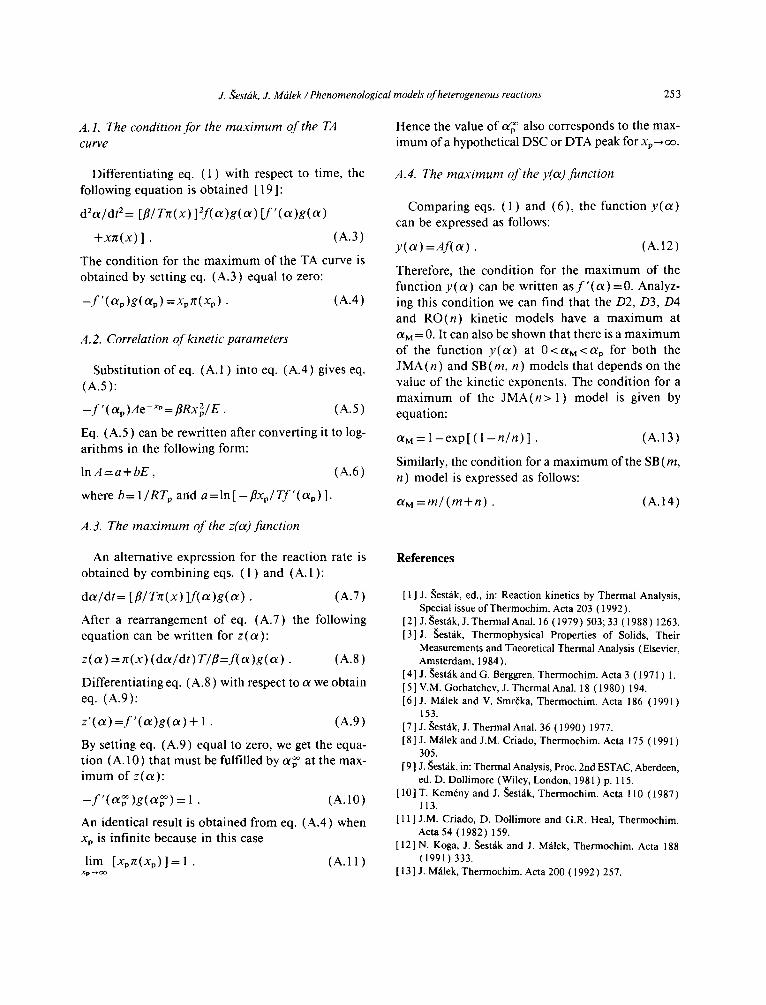
A. 1. The condition for the m a x i m u m o f the TA c u r v e

Hence the value of a ~ also corresponds to the max- imum of a hypothetical DSC or DTA peak for xp-- .~ .

Differentiat ing eq. (1) with respect to t ime, the following equat ion is obta ined [ 19 ]:

d 2 a / d t 2 = [fl/ Trc(x) ]2f( a )g( a ) [ f ' ( a )g( a )

+ x n ( x ) ] . (A.3)

The condi t ion for the m a x i m u m of the TA curve is obta ined by setting eq. (A.3) equal to zero:

- f ' ( a p ) g ( a p ) =XpTt(Xp) . (A.4)

A.2. Correlation o f kinetic parameters

Subst i tut ion o feq . (A.1) into eq. (A.4) gives eq. (A.5) :

- f ' ( ap)Ae . . . . f lRx~/ E . ( A.5 )

Eq. (A.5) can be rewrit ten after convert ing it to log- ar i thms in the following form:

l n A = a + b E , (A.6)

where b = 1/RTp and a = l n [ --flXp/Tf'(ap)].

A.3. The m a x i m u m o f the z(a) function

A.4. The m a x i m u m o f the y(a) function

Compar ing eqs. ( i ) and (6) , the function y ( a ) can be expressed as follows:

y ( a ) = A f ( a ) . (A.12)

Therefore, the condi t ion for the ma x imum of the function y ( a ) can be writ ten a s f ' ( a ) = 0 . Analyz- ing this condi t ion we can find that the D2, D3, D4 and R O ( n ) kinetic models have a ma x imum at aM = 0. It can also be shown that there is a ma x imum of the function y ( a ) at 0 < a M < a p for both the J M A ( n ) and SB(m, n) models that depends on the value of the kinetic exponents. The condi t ion for a ma x imum of the J M A ( n > 1) model is given by equation:

aM = 1 - e x p [ ( 1 - n / n ) ] . (A.13)

Similarly, the condit ion for a maximum of the SB (m, n) model is expressed as follows:

aM = m / ( m + n ) . (A.14)

An al ternat ive expression for the react ion rate is obta ined by combining eqs. ( 1 ) and (A.1) :

d o t / d t = [ f l / T n ( x ) ]f( a ) g ( ot) . (A.7)

After a rearrangement of eq. (A.7) the following equat ion can be writ ten for z ( a ) :

z ( a ) = n ( x ) ( d a / d t ) T / f l = f ( a ) g ( a ) . (A.8)

Differentiat ing eq. (A.8) with respect to a we obtain eq. (A.9) :

z ' ( a ) = f ' ( a ) g ( a ) + 1 . (A.9)

By setting eq. (A.9) equal to zero, we get the equa- tion (A. 10) that must be fulfilled by a ~ at the max- imum of z ( a ) :

- f ( a o ) g ( a p ) = 1 . (A.10)

An identical result is obta ined from eq. (A.4) when Xp is infinite because in this case

l im [ X p T ~ ( X p ) ] = 1 . (A.1 1) x l a ~

References

[ 1 ] J. ~esVik, ed., in: Reaction kinetics by Thermal Analysis, Special issue of Thermochim. Acta 203 ( 1992 ).

[ 2 ] J. ~est~ik, J. Thermal Anal. 16 ( 1979 ) 503; 33 ( 1988 ) 1263. [3] J. ~esuik, Thermophysical Properties of Solids, Their

Measurements and Theoretical Thermal Analysis (Elsevier, Amsterdam, 1984).

[4] J. ~est~ik and G. Berggren, Thermochim. Acta 3 ( 1971 ) I. [ 5 ] V.M. Gorbatchev, J. Thermal Anal. 18 (1980) 194. [6] J. M~llek and V. Smr6ka, Thermochim. Acta 186 (1991)

153. [7] J. ~est~ik, J. Thermal Anal. 36 (1990) 1977. [ 8 ] J. M~ilek and J.M. Criado, Thermochim. Acta 175 ( 1991 )

305. [9 ] J. ~est~ik, in: Thermal Analysis, Proc. 2nd ESTAC, Aberdeen,

ed. D. Dollimore (Wiley, London, 1981 ) p. 115. [ 10] T. Kem6ny and J. ~est~ik, Thermochim. Acta 110 (1987)

113. [ 11 ] J.M. Criado, D. Dollimore and G.R. Heal, Thermochim.

Acta 54 (1982) 159. [12] N. Koga, J. ~est~tk and J. M~ilek, Thermochim. Acta 188

(1991) 333. [ 13 ] J. M~llek, Thermochim. Acta 200 ( 1992 ) 257.

254 J. ~estdtk, J. M~lek / Phenomenological models of heterogeneous reactions

[ 14 ] G.I. Senum and R.T. Yang, J. Thermal Anal. 11 (1977) 445. [ 15 ] J.M. Criado, J. M~ilek and A. Ortega, Thermochim. Acta

147 (1989) 377. [ 16 ] J. M~ilek and J.M. Criado, Thermochim. Acta 164 (1990)

199. [ 17 ] E.S. Freeman and B. Carroll, J. Phys. Chem. 62 ( 1958 ) 394. [ 18 ] L. Tich~' and P. Nagels, Phys. Status Solidi A87 ( 1988 ) 769. [ 19] J. M~ilek, J. Non-Cryst. Solids 107 (1989) 323. [ 20 ] N. Koga and J. ~est~ik, Thermochim. Acta 182 ( 1991 ) 201. [ 21 ] J. ~est/ik, Phys. Chem. Glasses 15 (1974) 137. [22] J. ~est~ik, Thermochim. Acta 98 (1986) 339. [23] N. Koga and J. ~est~ik, J. Thermal Anal. 37 ( 1991 ) 1103. [24] J. M~llek, J.M. Criado, J. ~est~lk and J. Militk~,, Thermochim.

Acta 153 (1989)429.

[25 ] H.E. Kissinger, Anal. Chem. 29 (1957) 1702. [26] T. Ozawa, J. Thermal Anal. 2 (1979) 301. [27] J.M. Criado, J. Malek and A. Ortega, Thermochim. Acta

147 (1989) 377. [ 28 ] J. M~ilek, Thermochim. Acta 138 ( 1989 ) 337. [29] J. M~ilek and V. Smr?zka, Thermochim. Acta 186 (1991)

153. [30] J. M~ilek, J. Non-Cryst. Solids 107 (1989) 323. [31 ] V. ~atava, Thermochim. Acta 2 ( 1971 ) 423. [ 32 ] J. M~ilek, J.~est~ik, F. Rouquerol, J. Rouquerol, J.M. Criado

and A. Ortega, J. Thermal Anal. 38 (1992) 71.