192
| Date post: | 28-Oct-2015 |
| Category: |
Documents |
| Upload: | adriana-araujo |
| View: | 79 times |
| Download: | 4 times |

This page intentionally left blank
K I N K S A N D D O M A I N W A L L SAn Introduction to Classical and Quantum Solitons
Kinks and domain walls are the simplest kind of solitons and hence they are in-valuable for testing various ideas and for learning about non-perturbative aspectsof field theories. They are the subject of research in essentially every branch ofphysics, ranging from condensed matter to cosmology.
This book is a pedagogical introduction to kinks and domain walls and their prin-cipal classical and quantum properties. The book starts out by discussing classicalsolitons, building up from examples in elementary systems to more complicatedsettings. The quantum properties are introduced, together with discussion of thevery fundamental role that solitons may play in particle physics. The formation ofsolitons in phase transitions, their dynamics, and their cosmological consequencesare further discussed. The book closes with an explicit description of a few labora-tory systems containing solitons.
Kinks and Domain Walls includes several state-of-the-art results (some previ-ously unpublished), providing a handy reference. Each chapter closes with a list ofopen questions and research problems. This book will be of great interest to bothgraduate students and academic researchers in theoretical physics, particle physicsand condensed matter physics.
Tanmay Vachaspati is a professor in the Physics Department at Case WesternReserve University. He was the Rosenbaum Fellow for the Topological DefectsProgramme at the Isaac Newton Institute, and is a Fellow of the American PhysicalSociety. Professor Vachaspati co-edited The Formation and Evolution of CosmicStrings with Professors Gary Gibbons and Stephen Hawking.


KINKS AND DOMAIN WALLS
An Introduction to Classical and Quantum Solitons
T A N M A Y V A C H A S P A T ICase Western Reserve University
cambridge university pressCambridge, New York, Melbourne, Madrid, Cape Town, Singapore, São Paulo
Cambridge University PressThe Edinburgh Building, Cambridge cb2 2ru, UK
First published in print format
isbn-13 978-0-521-83605-0
isbn-13 978-0-511-24515-2
© T. Vachaspati 2006
2006
Information on this title: www.cambridg e.org /9780521836050
This publication is in copyright. Subject to statutory exception and to the provision ofrelevant collective licensing agreements, no reproduction of any part may take placewithout the written permission of Cambridge University Press.
isbn-10 0-511-24515-7
isbn-10 0-521-83605-0
Cambridge University Press has no responsibility for the persistence or accuracy of urlsfor external or third-party internet websites referred to in this publication, and does notguarantee that any content on such websites is, or will remain, accurate or appropriate.
Published in the United States of America by Cambridge University Press, New York
www.cambridge.org
hardback
eBook (EBL)
eBook (EBL)
hardback

dedicated to my mother’s memory
for Ramnath’s children(those who survived)


Contents
Preface page xi1 Classical kinks 1
1.1 Z2 kink 21.2 Rescaling 61.3 Derrick’s argument 61.4 Domain walls 71.5 Bogomolnyi method for Z2 kink 71.6 Z2 antikink 81.7 Many kinks 91.8 Inter-kink force 101.9 Sine-Gordon kink 121.10 Topology: π0 141.11 Bogomolnyi method revisited 171.12 On more techniques 181.13 Open questions 19
2 Kinks in more complicated models 202.1 SU (5) model 212.2 SU (5) × Z2 symmetry breaking and topological kinks 222.3 Non-topological SU (5) × Z2 kinks 262.4 Space of SU (5) × Z2 kinks 272.5 Sn kinks 282.6 Symmetries within kinks 292.7 Interactions of static kinks in non-Abelian models 312.8 Kink lattices 322.9 Open questions 34
3 Interactions 353.1 Breathers and oscillons 353.2 Kinks and radiation 38
vii

viii Contents
3.3 Structure of the fluctuation Hamiltonian 393.4 Interaction of kinks and radiation 403.5 Radiation from kink deformations 423.6 Kinks from radiation 453.7 Scattering of kinks 453.8 Intercommuting of domain walls 483.9 Open questions 48
4 Kinks in quantum field theory 504.1 Quantization of kinks: broad outline 514.2 Example: Z2 kink 584.3 Example: sine-Gordon kink 604.4 Quantized excitations of the kink 624.5 Sign of the leading order correction 634.6 Boson-fermion connection 654.7 Equivalence of sine-Gordon and massive Thirring models 674.8 Z2 kinks on the lattice 704.9 Comments 704.10 Open questions 71
5 Condensates and zero modes on kinks 735.1 Bosonic condensates 745.2 Fermionic zero modes 765.3 Fractional quantum numbers 815.4 Other consequences 825.5 Condensates on SU (5) × Z2 kinks 845.6 Possibility of fermion bound states 885.7 Open questions 89
6 Formation of kinks 906.1 Effective potential 906.2 Phase dynamics 936.3 Kibble mechanism: first-order phase transition 956.4 Correlation length 976.5 Kibble-Zurek mechanism: second-order phase transition 1016.6 Domain wall network formation 1056.7 Formation of S5 × Z2 domain wall network 1076.8 Biased phase transitions 1106.9 Open questions 112
7 Dynamics of domain walls 1137.1 Kinks in 1 + 1 dimensions 1137.2 Walls in 3 + 1 dimensions 1167.3 Some solutions 118
Contents ix
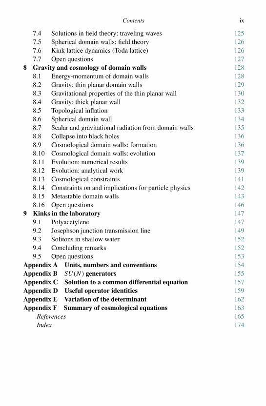
7.4 Solutions in field theory: traveling waves 1257.5 Spherical domain walls: field theory 1267.6 Kink lattice dynamics (Toda lattice) 1267.7 Open questions 127
8 Gravity and cosmology of domain walls 1288.1 Energy-momentum of domain walls 1288.2 Gravity: thin planar domain walls 1298.3 Gravitational properties of the thin planar wall 1308.4 Gravity: thick planar wall 1328.5 Topological inflation 1338.6 Spherical domain wall 1348.7 Scalar and gravitational radiation from domain walls 1358.8 Collapse into black holes 1368.9 Cosmological domain walls: formation 1368.10 Cosmological domain walls: evolution 1378.11 Evolution: numerical results 1398.12 Evolution: analytical work 1398.13 Cosmological constraints 1418.14 Constraints on and implications for particle physics 1428.15 Metastable domain walls 1438.16 Open questions 146
9 Kinks in the laboratory 1479.1 Polyacetylene 1479.2 Josephson junction transmission line 1499.3 Solitons in shallow water 1529.4 Concluding remarks 1529.5 Open questions 153
Appendix A Units, numbers and conventions 154Appendix B SU (N ) generators 155Appendix C Solution to a common differential equation 157Appendix D Useful operator identities 159Appendix E Variation of the determinant 162Appendix F Summary of cosmological equations 163
References 165Index 174


Preface
Solitons were first discovered by a Scottish engineer, J. Scott Russell, in 1834 whileriding his horse by a water channel when a boat suddenly stopped. A hump of waterrolled off the prow of the boat and moved rapidly down the channel for several miles,preserving its shape and speed. The observation was surprising because the humpdid not rise and fall, or spread and die out, as ordinary water waves do.
In the 150 years or so since the discovery of Scott Russell, solitons have beendiscovered in numerous systems besides hydrodynamics. Probably the most im-portant application of these is in the context of optics where they can propagatein optical fibers without distortion: they are being studied for high-data-rate (tera-bits) communication. Particle physicists have realized that solitons may also existin their models of fundamental particles, and cosmologists have realized that suchhumps of energy may be propagating in the far reaches of outer space. There is evenspeculation that all the fundamental particles (electrons, quarks etc.) may be viewedas solitons owing to their quantum properties, leading to a “dual” description offundamental matter.
In this book I describe the simplest kinds of solitons, called “kinks” in onespatial dimension and “domain walls” in three dimensions. These are also humpsof energy as in Scott Russell’s solitons. However, they also have a topologicalbasis that is absent in hydrodynamical solitons. This leads to several differencese.g. water solitons cannot stand still and have to propagate with a certain velocity,while domain walls can propagate with any velocity. Another important point in thisregard is that strict solitons, such as those encountered in hydrodynamics, preservetheir identity after scattering. The kinks and domain walls discussed in this bookdo not necessarily have this property, and can dissipate their energy on collision,and even annihilate altogether.
Why focus on kinks and domain walls? Because they are known to exist in manylaboratory systems and may exist in other exotic settings such as the early uni-verse. They provide a simple setting for discussing non-linear and non-perturbative
xi
xii Preface
physics. They can give an insight into the dynamics of phase transitions. Lessonslearned from the study of kinks and domain walls may also be applied to othermore complicated topological defects. Domain walls are good pedagogy as onecan introduce novel field theoretic, cosmological, and quantum issues without ex-traneous complexities that occur with their higher co-dimension defects (stringsand monopoles).
The chapters of this book can be approximately categorized under four differentheadings. The first two chapters discuss solitons as classical solutions, the nextthree describe their microscopic classical and quantum properties, followed byanother three chapters that discuss macroscopic properties and applications. Thevery last chapter discusses two real-world systems with kinks and, very briefly,Scott Russell’s soliton. The book should be accessible to a theoretically inclinedgraduate student, and a large part of the book should also be accessible to anadvanced undergraduate. At the end of every chapter, I have listed a few “openquestions” to inspire the reader to take the subject further. Some of these questionsare intentionally open-ended so as to promote greater exploration. Needless to say,there are no known answers to most of the open questions (that is why they are“open”) and the solutions to some will be fit to print.
Every time I think about research in this area, I feel very fortunate for havingunwittingly chosen it, for my journey on the “soliton train” has weaved througha vast landscape of physical phenomena, each with its own flavor, idiosyncrasies,and wonder. I hope that this book, as it starts out in classical solitons, then moveson to quantum effects, phase transitions, gravitation, and cosmology, and a bit ofcondensed matter physics, has captured some of that wonder for the reader.
This is not the first book on solitons and hopefully not the last one either. Inthis book I have presented a rather personal perspective of the subject, with someeffort to completeness but focusing on topics that have intrigued me. Throughout, Ihave included some material that is not found in the published literature. Prominentamong these is Section 4.5, where it is shown that the leading quantum correctionto the kink mass is negative. The discussion of Section 6.5, with its emphasis ona bifurcation of correlation scales, also expresses a new viewpoint. I had partic-ular difficulty deciding whether to include or omit discussion of domain walls insupersymmetric theories. On the one hand, many beautiful results can be derivedfor supersymmetric domain walls. On the other, the high degree of symmetry iscertainly not realized (or is broken) in the real world. Also, non-supersymmetricdomain walls are less constrained by symmetries and hence have richer possibilities.In the end, I decided not to include a discussion of supersymmetric walls, notingthe excellent review by David Tong (see below). Some other must-read referencesare:
Preface xiii
1. Rajaraman, R. (1982). Solitons and Instantons. Amsterdam: North-Holland.2. Rebbi, C. and Soliani, G. (1984). Solitons and Particles. Singapore: World Scientific.3. Coleman, S. (1985). Aspects of Symmetry. Cambridge: Cambridge University Press.4. Vilenkin, A. and Shellard, E. P. S. (1994). Cosmic Strings and Other Topological Defects.
Cambridge: Cambridge University Press.5. Hindmarsh, M. B. and Kibble, T. W. B. (1995). Cosmic Strings. Rep. Prog. Phys., 58,
477–562.6. Arodz, H., Dziarmaga, J. and Zurek, W. H., eds. (2003). Patterns of Symmetry Breaking.
Dordrecht: Kluwer Academic Publishers.7. Volovik, G. E. (2003). The Universe in a Helium Droplet. Oxford: Oxford University
Press.8. Manton, N. and Sutcliffe, P. (2004). Topological Solitons. Cambridge: Cambridge Uni-
versity Press.9. Tong, D. (2005). TASI Lectures on Solitons, [hep-th/0509216].
I am grateful to a number of experts who, over the years, knowingly or un-knowingly, have shaped this book. Foremost among these are my physicist father,Vachaspati, and Alex Vilenkin, my Ph.D. adviser. This book would not have beenwritten without the support of other experts who have collaborated with me in re-searching many of the topics that are covered in this book. These include: NunoAntunes, Harsh Mathur, Levon Pogosian, Dani Steer, and Grisha Volovik. Over theyears, several of the sections in the book have been influenced by conversationswith, and in some cases, owe their existence to, Sidney Coleman, Gary Gibbons,Tom Kibble, Hugh Osborn, and Paul Sutcliffe. The book would have many moreerrors, were it not for comments by Harsh Mathur, Ray Rivers, Dejan Stojkovic,Alex Vilenkin, and, especially, Dani Steer who painstakingly went over the bulk ofthe manuscript, making it much more readable and correct. My colleagues, CraigCopi and Pete Kernan, have provided invaluable computer support needed in thepreparation of this book. I thank the editorial staff at C.U.P. for their patience andprofessionalism, and the Universities of Paris (VII and XI) and the Aspen Centerfor Physics for providing very hospitable and conducive working environments.
As I learned, writing a book takes a lot of sacrifices, and my admiration for myfamily, with their happy willingness to tolerate this effort, has increased many-fold.This book could not have been written without the unflinching support of my wife,Punam, and the total understanding of my children, Pranjal and Krithi.


1
Classical kinks
Kink solutions are special cases of “non-dissipative” solutions, for which the energydensity at a given point does not vanish with time in the long time limit. On thecontrary, a dissipative solution is one whose energy density at any given locationtends to zero if we wait long enough [35],
limt→∞ maxxT00(t, x) = 0, dissipative solution (1.1)
where T00(t, x) is the time-time component of the energy-momentum tensor, orthe energy density, and is assumed to satisfy T00 ≥ 0. Dissipationless solutions arespecial because they survive indefinitely in the system.
In this book we are interested in solutions that do not dissipate. In fact, forthe most part, the solutions we discuss are static, though in a few cases we alsodiscuss field configurations that dissipate. However, in these cases the dissipationis very slow and hence it is possible to treat the dissipation as a small perturbation.In addition to being dissipationless, kinks are also characterized by a topologicalcharge. Just like electric charge, topological charge is conserved and this leads toimportant quantum properties.
In this chapter, we begin by studying kinks as classical solutions in certain fieldtheories, and devise methods to find such solutions. The simplest field theories thathave kink solutions are first described to gain intuition. These field theories are alsorealized in laboratory systems as we discuss in Chapter 9. The simple examplesset the stage for the topological classification of kinks and similar objects in higherdimensions (Section 1.10), and are valuable signposts in our discussion of the morecomplicated systems of Chapter 2.
1
2 Classical kinks
f
V(f)
−h 0 +h
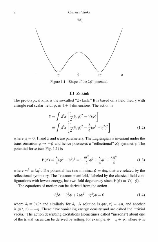
Figure 1.1 Shape of the λφ4 potential.
1.1 Z2 kink
The prototypical kink is the so-called “Z2 kink.” It is based on a field theory witha single real scalar field, φ, in 1 + 1 dimensions. The action is
S =∫
d2x
[1
2(∂µφ)2 − V (φ)
]
=∫
d2x
[1
2(∂µφ)2 − λ
4(φ2 − η2)2
](1.2)
where µ = 0, 1, and λ and η are parameters. The Lagrangian is invariant under thetransformation φ → −φ and hence possesses a “reflectional” Z2 symmetry. Thepotential for φ (see Fig. 1.1) is
V (φ) = λ
4(φ2 − η2)2 = −m2
2φ2 + λ
4φ4 + λη4
4(1.3)
where m2 ≡ λη2. The potential has two minima: φ = ±η, that are related by thereflectional symmetry. The “vacuum manifold,” labeled by the classical field con-figurations with lowest energy, has two-fold degeneracy since V (φ) = V (−φ).
The equations of motion can be derived from the action
∂2t φ − ∂2
x φ + λ(φ2 − η2)φ = 0 (1.4)
where ∂t ≡ ∂/∂t and similarly for ∂x . A solution is φ(t, x) = +η, and anotheris φ(t, x) = −η. These have vanishing energy density and are called the “trivialvacua.” The action describing excitations (sometimes called “mesons”) about oneof the trivial vacua can be derived by setting, for example, φ = η + ψ , where ψ is
1.1 Z2 kink 3
the excitation field. Then
S =∫
d2x
[1
2(∂µψ)2 − m2
ψ
2ψ2 −
√λ
2mψψ3 − λ
4ψ4
](1.5)
where
mψ =√
2m (1.6)
is the mass of the meson.Next consider the situation in which different parts of space are in different
vacua. For example, φ(t, −∞) = −η and φ(t, +∞) = +η. In this case, the functionφ(t, x) has to go from−η to+η as x goes from−∞ to+∞. By continuity of the fieldthere must be at least one point in space, x0, such that φ(t, x0) = 0. Since V (0) = 0,there is potential energy in the vicinity of x0, and the energy of this state is notzero. The solution of the classical equation of motion that interpolates between thedifferent boundary conditions related by Z2 transformations is called the “Z2 kink.”
We might wonder why the Z2 kink cannot evolve into the trivial vacuum? Forthis to happen, the boundary condition at, say, x = +∞ would have to change in acontinuous way from +η to −η. However, a small deviation of the field at infinityfrom one of the two vacua costs an infinite amount of potential energy. This isbecause as φ is changed, the field in an infinite region of space lies at a non-zerovalue of the potential (see Fig. 1.1). Hence, there is an infinite energy barrier tochanging the boundary condition.1
A way to characterize the Z2 kink is to notice the presence of a conserved current
jµ = 1
2ηεµν∂νφ (1.7)
where µ, ν = 0, 1 and εµν is the antisymmetric symbol in two dimensions (ε01 =1). By the antisymmetry of εµν , it is clear that jµ is conserved: ∂µ jµ = 0. Hence
Q =∫
dx j0 = 1
2η[φ(x = +∞) − φ(x = −∞)] (1.8)
is a conserved charge in the model. For the trivial vacua Q = 0, and for the kink con-figuration described above Q = 1. So the kink configuration cannot relax into thevacuum – it is in a sector that carries a different value of the conserved “topologicalcharge.”
To obtain the field configuration with boundary conditions φ(±∞) = ±η, wesolve the equations of motion in Eq. (1.4). We set time derivatives to vanish since
1 In Chapter 2 we will come across an example where the vacuum manifold is a continuum and correspondinglythere is a continuum of boundary conditions that can be chosen as opposed to the discrete choice in the Z2 case.This will lead to some new considerations.

4 Classical kinks
we are looking for static solutions. Then, the kink solution is
φk(x) = η tanh
(√λ
2ηx
)(1.9)
In fact, one can Lorentz boost this solution to get
φk(t, x) = η tanh
(√λ
2ηX
)(1.10)
where
X ≡ x − vt√1 − v2
(1.11)
(Recall that we are working in units in which the speed of light is unity i.e. c = 1.)The solution in Eq. (1.10) represents a kink moving at velocity v.
Another class of solutions is obtained by translating the solution in Eq. (1.9)
φk(x ; a) = η tanh
(√λ
2η(x − a)
)(1.12)
It is easily checked that translations do not change the energy of the kink. This isoften stated as saying that the kink has a zero energy fluctuation mode (or simplya “zero mode”). To explain this statement, we need to consider small fluctuationsof the field about the kink solution, similar to Eq. (1.5). We now have
φ = φk(x) + ψ(t, x) (1.13)
where φk denotes the kink solution. The fluctuation field, ψ , obeys the linearizedequation
∂2t ψ − ∂2
x ψ + λ(3φ2
k − η2)ψ = 0 (1.14)
To find the fluctuation eigenmodes we set
ψ = e−iωt f (x) (1.15)
where f (x) obeys
−∂2x f + λ
(3φ2
k − η2) = ω2 f (1.16)
We will discuss all the solutions to this equation in Chapter 4. Here we focus on thetranslation mode. Since translations cost zero energy, there has to be an eigenmodewith ω = 0. This can be obtained by directly solving Eq. (1.16) or by noting thatfor small a, the solution in Eq. (1.12) can be Taylor expanded as
φk(x ; a) = φk(x ; a = 0) + adφk
dx
∣∣∣∣a=0
(1.17)
1.1 Z2 kink 5
-4 -2 2 4
-1
-0.5
0.5
1
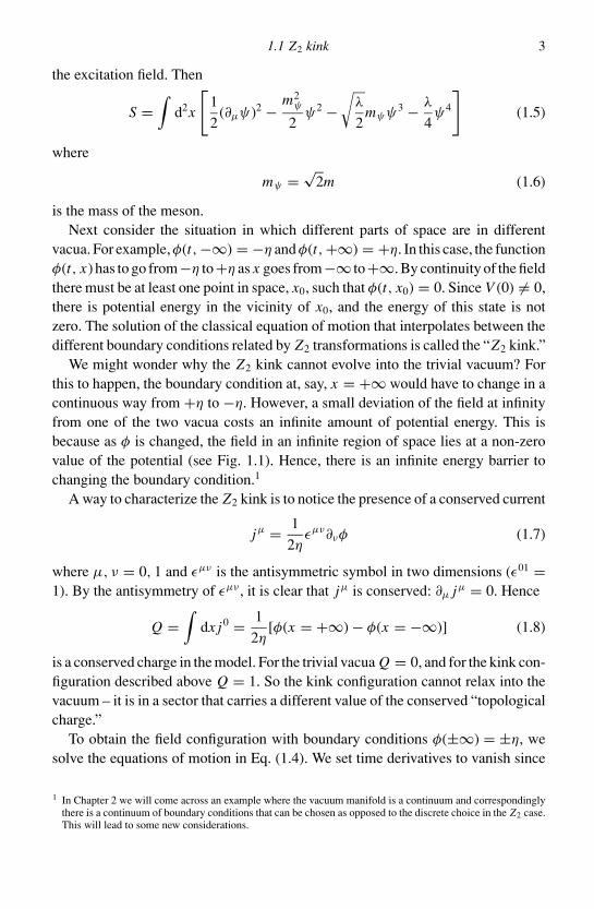
Figure 1.2 The curve ranging from −1 to +1 as x goes from −∞ to +∞ showsthe Z2 kink profile for λ = 2 and η = 1. The energy density of the kink has alsobeen plotted on the same graph for convenience, and to show that all the energy islocalized in the narrow region where the field has a gradient.
Comparing Eqs. (1.17) and (1.13), the zero mode solution is
f0(x) = dφk
dx
∣∣∣∣a=0
= η2
√λ
2sech2
(√λ
2ηx
)(1.18)
The solution in Eq. (1.9) can be used to calculate the energy density of the kink
E = 1
2(∂tφk)2 + 1
2(∂xφk)2 + V (φk)
= 0 + V (φk) + V (φk)
= λη4
2sech4
(√λ
2ηx
)(1.19)
where the second line is written to explicitly show that (∂xφ)2 = 2V (φ). The kinkprofile and the energy density are shown in Fig. 1.2. The total energy is
E =∫
dx E = 2√
2
3
m3
λ(1.20)
As is apparent from the solution and also the energy density profile, the half-width of the kink is,
w =√
2
λ
1
η=
√2
m= 2
mψ
(1.21)
On the x > 0 side of the kink we have φ ∼ +η while on the x < 0 side we haveφ ∼ −η. At the center of the kink, φ = 0, and hence the Z2 symmetry is restoredin the core of the kink. Therefore the interior of the kink is a relic of the symmetricphase of the system.
6 Classical kinks
1.2 Rescaling
It is convenient to rescale variables in the action in Eq. (1.2) as follows
= φ
η, yµ =
√λ ηxµ (1.22)
Then the rescaled action is
S = η2∫
d2 y
[1
2(∂µ)2 − 1
4(2 − 1)2
](1.23)
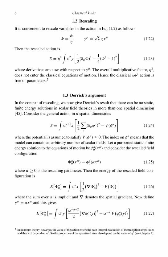
where derivatives are now with respect to yµ. The overall multiplicative factor, η2,does not enter the classical equations of motion. Hence the classical λφ4 action isfree of parameters.2
1.3 Derrick’s argument
In the context of rescaling, we now give Derrick’s result that there can be no static,finite energy solutions in scalar field theories in more than one spatial dimension[45]. Consider the general action in n spatial dimensions
S =∫
dn+1x
[1
2
∑a
(∂µφa)2 − V (φa)
](1.24)
where the potential is assumed to satisfy V (φa) ≥ 0. The index on φa means that themodel can contain an arbitrary number of scalar fields. Let a purported static, finiteenergy solution to the equations of motion be φa
0 (xµ) and consider the rescaled fieldconfiguration
a0(xµ) = φa
0 (αxµ) (1.25)
where α ≥ 0 is the rescaling parameter. Then the energy of the rescaled field con-figuration is
E[a
0
] =∫
dnx
[1
2
(∇a0
)2 + V(a
0
)](1.26)
where the sum over a is implicit and ∇ denotes the spatial gradient. Now defineyµ = αxµ and this gives
E[a
0
] =∫
dn y
[α−n+2
2
(∇φa0 (y)
)2 + α−n V(φa
0 (y))]
(1.27)
2 In quantum theory, however, the value of the action enters the path integral evaluation of the transition amplitudesand this will depend on η2. So the properties of the quantized kink also depend on the value of η2 (see Chapter 4).
1.5 Bogomolnyi method for Z2 kink 7
Since the kinetic terms are non-negative, we find that with n ≥ 2 and α > 1 thisgives
E[a
0
]< E
[φa
0
](1.28)
and hence φa0 cannot be an extremum of the energy. Only if n = 1 can φa
0 be a static,finite energy solution.
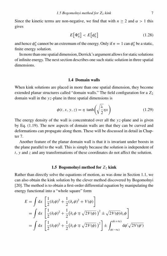
In more than one spatial dimension, Derrick’s argument allows for static solutionsof infinite energy. The next section describes one such static solution in three spatialdimensions.
1.4 Domain walls
When kink solutions are placed in more than one spatial dimension, they becomeextended planar structures called “domain walls.” The field configuration for a Z2
domain wall in the yz-plane in three spatial dimensions is
φ(t, x, y, z) = η tanh
(√λ
2ηx
)(1.29)
The energy density of the wall is concentrated over all the yz-plane and is givenby Eq. (1.19). The new aspects of domain walls are that they can be curved anddeformations can propagate along them. These will be discussed in detail in Chap-ter 7.
Another feature of the planar domain wall is that it is invariant under boosts inthe plane parallel to the wall. This is simply because the solution is independent oft , y and z and any transformations of these coordinates do not affect the solution.
1.5 Bogomolnyi method for Z2 kink
Rather than directly solve the equations of motion, as was done in Section 1.1, wecan also obtain the kink solution by the clever method discovered by Bogomolnyi[20]. The method is to obtain a first-order differential equation by manipulating theenergy functional into a “whole square” form
E =∫
dx
[1
2(∂tφ)2 + 1
2(∂xφ)2 + V (φ)
]
=∫
dx
[1
2(∂tφ)2 + 1
2
(∂xφ ∓
√2V (φ)
)2 ±√
2V (φ)∂xφ
]
=∫
dx
[1
2(∂tφ)2 + 1
2
(∂xφ ∓
√2V (φ)
)2]±∫ φ(+∞)
φ(−∞)dφ′√2V (φ′)
8 Classical kinks
Then, for fixed values of φ at ±∞, the energy is minimized if
∂tφ = 0 (1.30)
and
∂xφ ∓√
2V (φ) = 0. (1.31)
Further, the minimum value of the energy is
Emin = ±∫ φ(+∞)
φ(−∞)dφ′√2V (φ′). (1.32)
The energy can only be minimized provided a solution to Eq. (1.31) exists withthe correct boundary conditions. This relates the choice of sign in Eq. (1.31) tothe boundary conditions and to the sign in Eq. (1.32). In our case, for the Z2
kink boundary conditions (φ(+∞) > φ(−∞)), we take the − sign in Eq. (1.31).Inserting
√V (φ) =
√λ
4(η2 − φ2) (1.33)
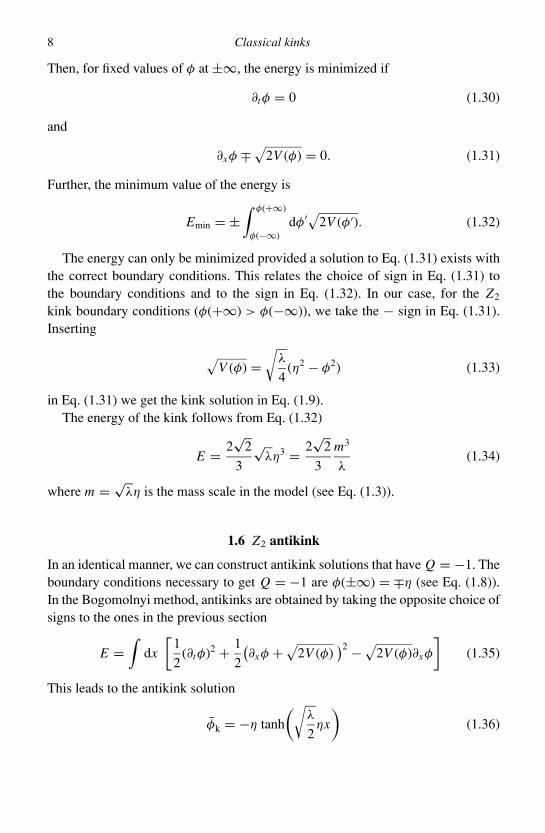
in Eq. (1.31) we get the kink solution in Eq. (1.9).The energy of the kink follows from Eq. (1.32)
E = 2√
2
3
√λη3 = 2
√2
3
m3
λ(1.34)
where m = √λη is the mass scale in the model (see Eq. (1.3)).
1.6 Z2 antikink
In an identical manner, we can construct antikink solutions that have Q = −1. Theboundary conditions necessary to get Q = −1 are φ(±∞) = ∓η (see Eq. (1.8)).In the Bogomolnyi method, antikinks are obtained by taking the opposite choice ofsigns to the ones in the previous section
E =∫
dx
[1
2(∂tφ)2 + 1
2
(∂xφ +
√2V (φ)
)2 −√
2V (φ)∂xφ
](1.35)
This leads to the antikink solution
φk = −η tanh
(√λ
2ηx
)(1.36)

1.7 Many kinks 9
1.7 Many kinks
The kink solution is well-localized and so it should be possible to write down fieldconfigurations with many kinks. However, a peculiarity of the Z2 kink system isthat a kink must necessarily be followed by an antikink since the asymptotic fieldsare restricted to lie in the vacuum: φ = ±η. It is not possible to have neighboringZ2 kinks or a system with topological charge |Q| > 1.
There is a simple scheme, called the “product ansatz,” to write down approxi-mate multi-kink field configurations, i.e. alternating kinks and antikinks. Supposewe have kinks at locations x = ki and antikinks at x = l j , where i, j label thevarious kinks and antikinks. The locations are assumed to be consistent with therequirement that kinks and antikinks alternate: . . . li < ki < li+1 . . . Then an ap-proximate field configuration that describes N kinks and N ′ antikinks is givenby the product of the solutions for the individual objects with a normalizationfactor
φ(x) = 1
ηN+N ′−1
N∏i=1
φk(x − ki )N ′∏
j=1
[−φk(x − l j )] (1.37)
where φk is the kink solution. Note that |N − N ′| ≤ 1 since kinks and antikinksmust alternate.
The product ansatz is a good approximation as long as the kinks are separatedby distances that are much larger than their widths. In that case, in the vicinity of aparticular kink, say at x = ki , only the factor φ(x − ki ) is non-trivial. All the otherfactors in Eq. (1.37) multiply together to give +1.
Another scheme to write down approximate multi-kink solutions is “additive”[109]. If φi denotes the i th kink (or antikink) in a sequence of N kinks and antikinks,we have
φ(x) =N∑
i=1
φi ± (N2 − 1)η, N2 = N (mod 2) (1.38)
where the sign is + if the leftmost object is a kink and − if it is an antikink.Neither the product or the additive ansatz yields a multi-kink solution to the
equations of motion. Instead they give field configurations that resemble severalwidely spaced kinks that have been patched together in a smooth way. If the multi-kink configuration given by either of the ansatze is evolved using the equation ofmotion, the kinks will start moving due to forces exerted by the other kinks. In thenext section we discuss the inter-kink forces.

10 Classical kinks
h
−a
−a + R
0
+a
x
f
−a − R
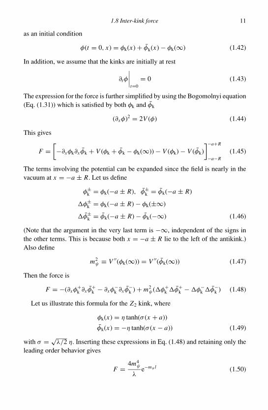
Figure 1.3 A widely separated kink-antikink.
1.8 Inter-kink force
Consider a kink at x = −a and an antikink at x = +a where the separation 2a ismuch larger than the kink width (see Fig. 1.3). We would like to evaluate the forceon the kink owing to the antikink [109].
The energy-momentum tensor for the action Eq. (1.2) with a general potentialV (φ) is
Tµν = ∂µφ∂νφ − gµν
1
2(∂αφ)2 − V (φ)
(1.39)
where gµν is the metric tensor that we take to be the flat metric, that is, gµν =diag(1, −1). The force exerted on a kink is given by Newton’s second law, bythe rate of change of its momentum. The momentum of a kink can be found byintegrating the kink’s momentum density, T 0i = −T0i , in a large region around thekink. If the kink is located at x = −a, let us choose to look at the momentum, P ,of the field in the region (−a − R, −a + R)
P = −∫ −a+R
−a−Rdx ∂tφ∂xφ (1.40)
After using the field equation of motion (for a general potential) and on performingthe integration, the force on the field in this region is
F = dP
dt=[−1
2(∂tφ)2 − 1
2(∂xφ)2 + V (φ)
]−a+R
−a−R
(1.41)
To proceed further we need to know the field φ in the interval (−a − R, −a + R).This may be obtained using the additive ansatz given in Eq. (1.38) which we take
1.8 Inter-kink force 11
as an initial condition
φ(t = 0, x) = φk(x) + φk(x) − φk(∞) (1.42)
In addition, we assume that the kinks are initially at rest
∂tφ
∣∣∣∣t=0
= 0 (1.43)
The expression for the force is further simplified by using the Bogomolnyi equation(Eq. (1.31)) which is satisfied by both φk and φk
(∂xφ)2 = 2V (φ) (1.44)
This gives
F =[−∂xφk∂x φk + V (φk + φk − φk(∞)) − V (φk) − V (φk)
]−a+R
−a−R
(1.45)
The terms involving the potential can be expanded since the field is nearly in thevacuum at x = −a ± R. Let us define
φ±k = φk(−a ± R), φ±
k = φk(−a ± R)
φ±k = φk(−a ± R) − φk(±∞)
φ±k = φk(−a ± R) − φk(−∞) (1.46)
(Note that the argument in the very last term is −∞, independent of the signs inthe other terms. This is because both x = −a ± R lie to the left of the antikink.)Also define
m2ψ ≡ V ′′(φk(∞)) = V ′′(φk(∞)) (1.47)
Then the force is
F = −(∂xφ+k ∂x φ
+k − ∂xφ
−k ∂x φ
−k ) + m2
ψ (φ+k φ+
k − φ−k φ−
k ) (1.48)
Let us illustrate this formula for the Z2 kink, where
φk(x) = η tanh(σ (x + a))
φk(x) = −η tanh(σ (x − a)) (1.49)
with σ = √λ/2 η. Inserting these expressions in Eq. (1.48) and retaining only the
leading order behavior gives
F = 4m4ψ
λe−mψ l (1.50)
12 Classical kinks
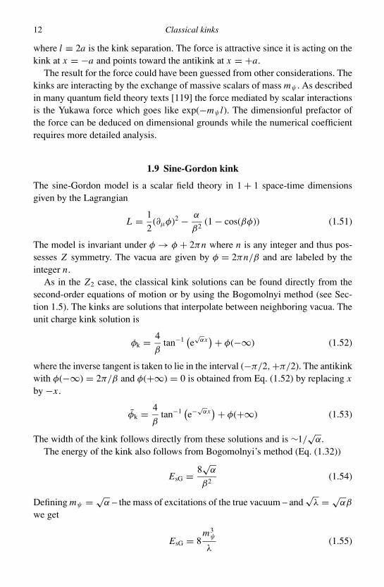
where l ≡ 2a is the kink separation. The force is attractive since it is acting on thekink at x = −a and points toward the antikink at x = +a.
The result for the force could have been guessed from other considerations. Thekinks are interacting by the exchange of massive scalars of mass mψ . As describedin many quantum field theory texts [119] the force mediated by scalar interactionsis the Yukawa force which goes like exp(−mψ l). The dimensionful prefactor ofthe force can be deduced on dimensional grounds while the numerical coefficientrequires more detailed analysis.
1.9 Sine-Gordon kink
The sine-Gordon model is a scalar field theory in 1 + 1 space-time dimensionsgiven by the Lagrangian
L = 1
2(∂µφ)2 − α
β2(1 − cos(βφ)) (1.51)
The model is invariant under φ → φ + 2πn where n is any integer and thus pos-sesses Z symmetry. The vacua are given by φ = 2πn/β and are labeled by theinteger n.
As in the Z2 case, the classical kink solutions can be found directly from thesecond-order equations of motion or by using the Bogomolnyi method (see Sec-tion 1.5). The kinks are solutions that interpolate between neighboring vacua. Theunit charge kink solution is
φk = 4
βtan−1
(e√
αx)+ φ(−∞) (1.52)
where the inverse tangent is taken to lie in the interval (−π/2, +π/2). The antikinkwith φ(−∞) = 2π/β and φ(+∞) = 0 is obtained from Eq. (1.52) by replacing xby −x .
φk = 4
βtan−1
(e−√
αx)+ φ(+∞) (1.53)
The width of the kink follows directly from these solutions and is ∼1/√
α.The energy of the kink also follows from Bogomolnyi’s method (Eq. (1.32))
EsG = 8√
α
β2(1.54)
Defining mψ = √α – the mass of excitations of the true vacuum – and
√λ = √
αβ
we get
EsG = 8m3
ψ
λ(1.55)
1.9 Sine-Gordon kink 13
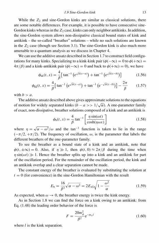
While the Z2 and sine-Gordon kinks are similar as classical solutions, thereare some notable differences. For example, it is possible to have consecutive sine-Gordon kinks whereas in the Z2 case, kinks can only neighbor antikinks. In addition,the sine-Gordon system allows non-dissipative classical bound states of kink andantikink – the so-called “breather” solutions – while no such solutions are knownin the Z2 case (though see Section 3.1). The sine-Gordon kink is also much moreamenable to a quantum analysis as we discuss in Chapter 4.
We can use the additive ansatz described in Section 1.7 to construct field configu-rations for many kinks. Specializing to a kink-kink pair (φ(−∞) = 0 to φ(+∞) =4π/β) and a kink-antikink pair (φ(−∞) = 0 and back to φ(+∞) = 0), we have
φkk(t, x) = 4
β
[tan−1
(e√
α(x−a))+ tan−1
(e√
α(x−b))]
(1.56)
φkk(t, x) = 4
β
[tan−1
(e√
α(x−a))+ tan−1
(e−√
α(x−b))]− 2π
β(1.57)
with b > a.The additive ansatz described above gives approximate solutions to the equations
of motion for widely separated kinks (b − a >> 1/√
α). A one-parameter familyof exact, non-dissipative, breather solutions composed of a kink and an antikink is
φb(t, x) = 4
βtan−1
[η sin(ωt)
cosh(ηωx)
](1.58)
where η = √α − ω2/ω and the tan−1 function is taken to lie in the range
(−π/2, +π/2). The frequency of oscillation, ω, is the parameter that labels thedifferent breathers of the one-parameter family.
To see the breather as a bound state of a kink and an antikink, note thatφ(t, ±∞) = 0. Also, if η 1, then φ(t, 0) ≈ 2π/β during the time whenη sin(ωt) 1. Hence the breather splits up into a kink and an antikink for partof the oscillation period. For the remainder of the oscillation period, the kink andan antikink overlap and a clear separation cannot be made.
The constant energy of the breather is evaluated by substituting the solution att = 0 (for convenience) in the sine-Gordon Hamiltonian with the result
Eb = 16
β2
√α − ω2 = 2EsG
√1 − ω2
α(1.59)
As expected, when ω → 0, the breather energy is twice the kink energy.As in Section 1.8 we can find the force on a kink owing to an antikink: from
Eq. (1.48) the leading order behavior of the force is
F = 20m2ψ
β2e−mψ l (1.60)
where l is the kink separation.

14 Classical kinks
1.10 Topology: π0
The kinks in the Z2 and sine-Gordon models can be viewed as arising purelyfor topological reasons, as we now explain. A very important advantage of thetopological viewpoint is that it is generalizable to a wide variety of models andcan be used to classify a large set of solutions. When applied to field theories inhigher spatial dimensions, topological considerations are convenient in order todemonstrate the existence of solutions such as strings and monopoles.
Consider a field theory for a set of fields denoted by Φ that is invariant undertransformations belonging to a group G. This means that the Hamiltonian of thetheory is invariant under G:
H[Φ] = H[Φg] (1.61)
where g ∈ G and Φg represents Φ after it has been transformed by the action ofg. The group G is a symmetry of the system, if Eq. (1.61) holds for every g ∈ Gand for every possible Φ. Now, let the Hamiltonian be minimized when Φ = Φ0.Then, from Eq. (1.61), it is also minimized with Φ = Φg
0 for any g ∈ G, and themanifold of lowest energy states – “vacuum manifold” – is labeled by the set offield configurations Φg
0. However, there will exist a subgroup (sometimes trivial),H of G, whose elements do not move Φ0:
Φh0 = Φ0 (1.62)
Hence, a group element gh ∈ G acting on Φ0 has the same result as g acting onΦ0 (because h acts first and does not move Φ0). So, while the configuration Φg
0
has the same energy as Φ0 for any g, not all the Φg0s are distinct from each other.
The distinct Φg0s are labeled by the set of elements gh : h ∈ H ≡ gH . The set
of elements gH : g ∈ G are said to form a “coset space” and the set is denotedby G/H ; each element of the space is a coset (more precisely a “left coset” sinceg multiplies H from the left). Therefore the vacuum manifold is isomorphic to thecoset space G/H .
We have so far connected the symmetries of the model to the vacuum manifold.Now we discuss the tools for describing the topology of the vacuum manifold. Thiswill lead to a description of the topology of the vacuum manifold directly in termsof the symmetries of the model.
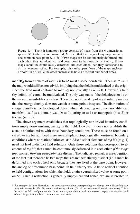
The topology of a manifold, M , is classified by the homotopy groups, πn(M ; x0),n = 0, 1, 2,. . . The idea is to consider maps from n-spheres to M , with theimage of an n-sphere in M containing one common base point, x0 (see Fig. 1.4).If two maps can be continuously deformed into each other, they are consideredto be topologically equivalent. In this way, the set of maps is divided into equiva-lence classes of maps, where each equivalence class contains the set of maps that

1.10 Topology: π0 15
are continuously deformable into each other. The elements of πn(M ; x0) are theequivalence classes of maps from Sn to M with fixed base point. It is also possibleto define (except for n = 0 as explained below) a suitable “product” of two maps:essentially the product of maps f and g (denoted by g · f ) and is defined to be“ f composed with g” or “ f followed by g.” Then it is easily verified that the prod-uct is closed, associative, an identity map exists, and every map has an inverse. Inmathematical language, ∀ f, g, h ∈ G,
f · g ∈ G
f · (g · h) = ( f · g) · h
∃ e ∈ G such that f · e = e · f = f
∃ f −1 ∈ G such that f · f −1 = f −1 · f = e (1.63)
Thus all the group properties are satisfied and πn(M ; x0) is a group.Two homotopy groups with different base points, say πn(M ; x0) and πn(M ; x ′
0),can be shown to be isomorphic and hence the reference to the base point is oftendropped and the homotopy group simply written as πn(M). Mathematicians havecalculated the homotopy groups for a wide variety of manifolds and this makes itvery convenient to determine if a given symmetry breaking leads to a topologicallynon-trivial vacuum manifold [145, 3, 171].
In the case of kinks or domain walls, the field defines a mapping from thepoints x = ±∞ to the vacuum manifold. Hence the relevant homotopy “group” isπ0(M ; x0), which contains maps from S0 (a point) to M . Since the base point is fixed,the image of either of the two possible S0s (x = ±∞) has to be x0, and π0(M ; x0)is trivial. Even if we do not impose the restriction that the maps should have a fixedbase point, it is not possible to define a suitable composition of maps. Therefore π0
does not have the right group structure and should merely be considered as a set ofmaps from S0 to the vacuum manifold. The exception occurs if M = G/H is itselfa group, which occurs when H is a normal subgroup of G, because then π0(M) caninherit the group structure of M . In this case, the product of two maps from S0 toM can be defined to be the map from S0 to the product of the two image points inM . Generally, however, π0(M) should simply be thought of as a set of maps fromS0 to the various disconnected pieces of M .
To connect the elements of the homotopy groups to topological field config-urations assume that the field, Φ, is in the vacuum manifold on Sn
∞. Therefore,Φ∞ ≡ Φ(x ∈ Sn
∞) defines a map from Sn to the vacuum manifold and this map canbe topologically non-trivial if πn(M) is non-trivial. We want to show that if the mapΦ∞ is topologically non-trivial, Φ cannot be in the vacuum manifold at all pointsin the interior of Sn
∞. Consider what happens as the radius of Sn∞ is continuously
decreased. If the field remains on the vacuum manifold, continuity implies that the
16 Classical kinks
Sn
x0
M
Figure 1.4 The nth homotopy group consists of maps from the n-dimensionalsphere, Sn , to the vacuum manifold, M , such that the image of any map containsone common base point x0 ∈ M . If two maps can be continuously deformed intoeach other, they are identified, and correspond to the same element of πn . If twomaps cannot be continuously deformed into each other, then they correspond todistinct elements of πn . For example, this can happen if one of the maps enclosesa “hole” in M , while the other encloses the hole a different number of times.
map ΦR from a sphere of radius R to M must also be non-trivial. Then as R → 0,the map would still be non-trivial, implying that the field is multivalued at the originsince the field must continue to map Sn
R non-trivially as R → 0. However, a field(by definition) cannot be multivalued. The only way out is if the field does not lie onthe vacuum manifold everywhere. Therefore non-trivial topology at infinity impliesthat the energy density does not vanish at some points in space. The distribution ofenergy density is the topological defect which, depending on dimensionality, canmanifest itself as a domain wall (n = 0), string (n = 1) or monopole (n = 2) ortexture (n = 3).
The above argument establishes that topologically non-trivial boundary condi-tions imply non-vanishing energy in the field. However, it does not establish thata static solution exists with those boundary conditions. These must be found on acase-by-case basis. Indeed there are examples of topologically non-trivial boundaryconditions where no static solution exists.3 Also distinct elements of πn(M) (n ≥ 1)need not lead to distinct field solutions. Only those solutions that correspond to el-ements of πn(M) that cannot be continuously deformed into each other, if the mapsare released from the base point, are distinct. The italicized remark is in recognitionof the fact that there can be two maps that are mathematically distinct (i.e. cannot bedeformed into each other) only because they are fixed at the base point. However,the analog of a “common base point” in field theory would be to restrict attentionto field configurations for which the fields attain a certain fixed value at some pointon Sn
∞. Such a restriction is generally unphysical and hence, we are interested in
3 For example, in three dimensions, the boundary conditions corresponding to a charge two ’t Hooft-Polyakovmagnetic monopole [124, 79] do not lead to any solution (for all but one value of model parameters). This isbecause any field configuration with those boundary conditions breaks up into two magnetic monopoles, eachof unit charge, that repel each other and are never static.

1.11 Bogomolnyi method revisited 17
maps that cannot be deformed into each other even if we release the restriction thatall maps have a common base point (for a more detailed discussion, see [171]).
In the case when the vacuum manifold has disconnected components, π0(G/H )is non-trivial since there are points (zero-dimensional spheres) that lie in differentcomponents that cannot be continuously deformed into one another. Therefore kinksoccur whenever π0(G/H ) is non-trivial. In the λΦ4 model, G = Z2, H = 1 andπ0(G/H ) = Z2. In the sine-Gordon model G = Z , H = 1 and π0(G/H ) = Z . Ifπ0 = Z N , we name the resulting kinks “Z N kinks.” In these simple examples, π0
forms a group because G is Abelian and so G/H itself is a group. An examplein which π0 is not a group can be constructed by choosing G = S3 (Sn is thepermutation group of n elements) broken down to H = S2.
The kinks in a model with disconnected elements in M can now be classified.Every element of π0(M) corresponds to a mapping from a point at spatial infinityto M and hence specifies a domain at infinity. Kinks occur if the domains at ±∞are distinct. Therefore pairs of elements of π0(M) classify domain walls.
1.11 Bogomolnyi method revisited
The Bogomolnyi method can be extended to include a large class of systems. Let usstart with the general energy functional for a matrix-valued complex scalar field Φ
E =∫
dx[Tr|∂t|2 + Tr|∂x|2 + V (, ∗)
]=∫
dx[∂t
∗ab∂tba + ∂x
∗ab∂xba + V (, ∗)
](1.64)
where a sum over matrix components labeled by a, b is understood. As in Sec-tion 1.5, we would like to write the energy density in “whole square” form
E =∫
dx[Tr|∂t|2 + |∂x ∓ U ()|2 ± (∂x
†U ) ± (U †∂x)] (1.65)
where we are restricting ourselves to static solutions and U is some matrix-valuedfunction of Φ such that
Tr(U †U ) = V (, ∗) (1.66)
The energy is minimized if
∂t = 0 (1.67)
and
Tr|∂x ∓ U (, ∗)|2 = 0 (1.68)
18 Classical kinks
which in turn gives
∂x ∓ U (, ∗) = 0 (1.69)
The energy of the kink is
E = ±∫ +∞
−∞dx Tr(∂x
† U + U †∂x) (1.70)
There is a further special case – the “supersymmetric” case – in which the energyintegral can be performed explicitly. This is if U is a total derivative
U ∗ = ∂W
∂(1.71)
where W (Φ,Φ∗) is the “superpotential,” assumed to be real. Then
E = ±∫ +∞
−∞dx Tr
(∂x
† ∂W
∂∗ + ∂xT ∂W
∂
)
= ±∫ +∞
−∞dx ∂x W
= ±[W ((+∞)) − W ((−∞))] (1.72)
Therefore we see that the Bogomolnyi method allows for first-order equationsof motion provided that V can be written as Tr(U †U ). The method also providesan explicit expression for the kink energy if V is given in terms of a superpotentialW as
V () = Tr(U †U ) = Tr
∣∣∣∣dW
d
∣∣∣∣2
(1.73)
1.12 On more techniques
The kink solutions we have been discussing fall under the more general categoryof “solitary waves,” often discussed under the soliton heading. Strictly speaking,for a solution to classify as a “soliton,” it also has to satisfy certain conditionson its scattering with other solitons. The subject is incredibly rich, and has led tothe development of very sophisticated mathematical techniques such as Backlundtransformations, inverse scattering methods, Lax heirarchy, etc. In addition, solitonshave found tremendous importance in physical applications, especially non-linearoptics and communication. Readers interested in the mathematics and physics ofsolitons might wish to consult [1, 48, 56].
Strict solitons are usually discussed in one spatial dimension and have limitedapplication in the context of particle physics. Nonetheless, there are equally so-phisticated techniques to study solitary wave solutions in higher dimensions. In
1.13 Open questions 19
particular, the ADHM construction [12] is used to find instanton solutions in fourspatial dimensions and the Nahm equations lead to magnetic monopole solutionsin three dimensions [114].
The soliton analyses mentioned above consider equations with complicated non-linear terms and higher derivatives. In the context of particle physics, such termsand derivatives are rarely encountered. However, one complication that arises isdue to larger (non-Abelian) symmetry groups. In the next chapter we will takethe analysis of this section to such particle-physics motivated models. There wewill find a spectrum of kink solutions with unusual interactions. As we proceed tofurther chapters, we will learn that the physics of such non-Abelian kinks can bequite different from that of the simple kinks discussed in this chapter.
1.13 Open questions
1. Discuss the conditions needed for a breather solution to exist. If an exact breather does notexist, can there be an approximate breather (see Section 3.1)? What is the approximation?
2
Kinks in more complicated models
The Z2 and sine-Gordon kinks discussed in the last chapter are not representative ofkinks in models where non-Abelian symmetries are present. Kinks in such modelshave more degrees of freedom and this introduces degeneracies when imposingboundary conditions, leading to many kink solutions with different internal struc-tures (but the same topology). Indeed, kink-like solutions may exist even when thetopological charge is zero. The interactions of kinks in these more complicatedmodels, their formation and evolution, plus their interactions with other particlesare very distinct from the kinks of the last chapter.
We choose to focus on kinks in a model that is an example relevant to particlephysics and cosmology. The model is the first of many Grand Unified Theories ofparticle physics that have been proposed [63]. The idea behind grand unificationis that Nature really has only one gauge-coupling constant at high energies, andthat the disparate values of the strong, weak, and electromagnetic coupling con-stants observed today are due to symmetry breaking and the renormalization-grouprunning of coupling constants down to low energies. Since there is only one gauge-coupling constant in these models, there is a simple grand unified symmetry groupG that is valid at high energies, for example, at the high temperatures present inthe very early universe. At lower energies, G is spontaneously broken in stages,eventually leaving only the presently known quantum chromo dynamics (QCD) andelectromagnetic symmetries SU (3)c × U (1)em of particle physics, with its two dif-ferent coupling constants. It can be shown [63] that the minimal possibility for G isSU (5). However, since Grand Unified Theories predict proton decay, experimentalobservation of the longevity of the proton (∼ 5 × 1033 years) leads to constraintson grand unified models. The (non-supersymmetric) SU (5) Grand Unified Theoryis ruled out by the current lower limits on the proton’s lifetime. Therefore particle-physics model builders consider yet larger groups G, or with an extended scalarfield sector, or supersymmetric extensions of SU (5), and other models based onlarger groups. Even if the symmetry group is larger than SU (5), it often happens
20
2.1 SU (5) model 21
that after a series of symmetry breaking, the residual symmetry is SU (5), whichthen proceeds to break to the current symmetry group. Hence the study of SU (5)symmetry breaking is extremely relevant to particle physics, even if it is not theultimate grand unified symmetry group.
In this chapter we shall study kinks in a model with SU (5) × Z2 symmetrythough almost all the discussion can be generalized to an SU (N ) × Z2 model forodd values of N [163, 120]. The extra Z2 symmetry is explained in the next section.Since we only desire to study kinks in a particle-physics motivated model, it wouldseem simpler to choose a model based on the smaller SU (3) group. However, itcan be shown that there is no way to construct a model with just SU (3) symmetryand with the simplest choice of field content, which is one adjoint field. Instead,the model must have the larger O(8) symmetry. Other fields need to be includedso as to reduce the O(8) to SU (3), but that introduces additional parameters whichmake the SU (3) model more messy than the SU (5) model.
Dealing with continuous groups such as SU (5) requires certain backgroundmaterial. The fundamental representation of SU (N ) generators is described in Ap-pendix B. A summary of some aspects of the SU (5) model of grand unification isgiven in Section 5.5.
2.1 SU (5) model
The SU (5) model can be written as1
L = Tr(Dµ)2 − 1
2Tr(Xµν Xµν) − V () (2.1)
where, in terms of components, is a scalar field (also called a Higgs field)transforming in the adjoint representation of SU (5), that is, → ′ = gg† forg ∈ SU (5). The gauge field strengths are Xµν = Xa
µνT a and the SU (5) generatorsT a are normalized such that Tr(T aT b) = δab/2. The definition of the covariantderivative is
Dµ = ∂µ − ieXµ (2.2)
and its action on the adjoint scalar is given by
Dµ = ∂µ − ie[Xµ, ] (2.3)
The gauge field strength is given in terms of the covariant derivative via
−ieXµν = [Dµ, Dν] (2.4)
1 We are using the Einstein summation convention in which repeated group and space-time indices are summedover. So, explicitly, =∑24
a=1 a T a . See Appendix B for more details on the SU (5) generators T a .
22 Kinks in more complicated models
and the potential is the most general quartic in
V () = −m2Tr(2) + h[Tr(2)]2 + λTr(4) + γ Tr(3) − V0 (2.5)
where V0 is a constant that is chosen so as to set the minimum value of the potentialto zero.
The model in Eq. (2.1) does not have any topological kinks because there areno broken discrete symmetries. In particular, the Z2 symmetry under → − isabsent owing to the cubic term in Eq. (2.5). Note that → − is not achievableby an SU (5) transformation. To show this, consider Tr(3). This is invariant underany SU (5) transformation, but not under → −. However, if γ = 0, there aretopological kinks connecting the two vacua related by → −. For non-zero butsmall γ , these kinks are almost topological. In our analysis in this chapter we setγ = 0, in which case the symmetry of the model is SU (5) × Z2. The philosophyunderlying grand unification does not forbid discrete symmetry factors since suchfactors do not entail additional gauge-coupling constants. Indeed, model buildersoften set γ = 0 for simplicity. Now a non-zero vacuum expectation value of
breaks the discrete Z2 factor leading to topological kinks.
2.2 SU (5) × Z2 symmetry breaking and topological kinks
The potential in Eq. (2.5) has a (degenerate) global minimum at
0 = η
2√
15diag(2, 2, 2, −3, −3) (2.6)
where η = m/√
λ′ provided
λ ≥ 0, λ′ ≡ h + 7
30λ ≥ 0 (2.7)
For the global minimum to have V (0) = 0, in Eq. (2.5) we set
V0 = −λ′
4η4 (2.8)
As discussed in Section 1.10, if we transform 0 by any element of SU (5) × Z2,the transformed 0 is still at a minimum of the potential. However, 0 is leftunmoved by transformations belonging to
G321 ≡ [SU (3) × SU (2) × U (1)]
Z3 × Z2(2.9)
where SU (3) acts on the upper-left 3 × 3 block of 0, SU (2) on the lower-right2 × 2 block, and U (1) is generated by 0 itself. Hence, G321 is the unbrokensymmetry group.

2.2 SU (5) × Z2 symmetry breaking and topological kinks 23
Φ (−)
Φ (+)
Figure 2.1 The vacuum manifold of the SU (5) × Z2 model consists of two dis-connected 12-dimensional copies. Kink solutions correspond to paths that originatein one piece at x = −∞, denoted by (−), leave the vacuum manifold, and endin the other disconnected piece at x = +∞. Topological considerations specifythat (+) has to lie in the disconnected piece on the right, but not where it shouldbe located within this piece.
SU (5) has 24 generators while the unbroken group, G321, has a total of 12generators, namely, 8 of SU (3), 3 of SU (2), and 1 of U (1). Therefore the vacuummanifold is 24 − 12 = 12 dimensional but in two disconnected pieces as depicted inFig. 2.1 because of the Z2 factor. Kink solutions occur if the boundary conditions liein different disconnected pieces. However, if we start at some point on the vacuummanifold at x = −∞, say (−∞) = −, we have a choice of boundary conditionsfor +, the vacuum expectation value of at x = +∞ (compare with the Z2 casewhere the path had to go from definite initial to definite final values of ).
We will narrow down the possible choices for + very shortly. First we point outthat the gauge fields can be set to zero in finding kink solutions [163]. To see thisexplicitly, the only linear term in the gauge field is ieTr(Xi [, ∂i]). However, oursolution for satisfies [, ∂i] = 0 [120] and so the variation vanishes to linearorder in gauge field fluctuations. A closer look also reveals that the quadratic termsof perturbations in the gauge fields contribute positively to the energy of the kinksolutions and so the gauge fields do not cause an instability of the solutions [163].Hence we set
Xµ = 0 (2.10)
As we now show, the boundary conditions that lead to static solutions of the equa-tions of motion are rather special [120].
Theorem: A static solution can exist only if [+, −] = 0.
We only give a sketch of the proof here since it is of a technical nature. Theessential idea is that if k(x) is a static solution, then the energy should be extrem-ized by it. By considering perturbations of the kind U (x)kU †(x) where U (x) is aninfinitesimal rotation of SU (5), one finds that the energy can be extremized only if

24 Kinks in more complicated models
[k, ∂xk] = 0 for all x . Now at large x , we have k → +. In this region ∂xk
has terms that are proportional to − as well, even if these are exponentially small,since (x) is an analytic function. Hence, a static solution requires [+, −] = 0.
The theorem immediately narrows down the possibilities that we need to considerwhen trying to construct kink solutions. If we fix
− = 0 = η
2√
15diag(2, 2, 2, −3, −3) (2.11)
+ can take on the following three values
(0)+ = − η
2√
15diag(2, 2, 2, −3, −3)
(1)+ = − η
2√
15diag(2, 2, −3, 2, −3)
(2)+ = − η
2√
15diag(2, −3, −3, 2, 2) (2.12)
One can also rotate these three choices by elements of the unbroken group G321−that leaves − invariant and obtain three disjoint classes of possible values of +.The three choices given above are representatives of their classes.
The kink solution for any of the three boundary conditions is of the form
φ(q)k = F (q)
+ (x)M(q)+ + F (q)
− (x)M(q)− + g(q)(x)M(q) (2.13)
where q = 0, 1, 2 labels the solution class,
M(q)+ =
(q)+ +
(q)−
2, M(q)
− = (q)+ −
(q)−
2(2.14)
and M(q) will be specified below.The boundary conditions for F (q)
± are
F (q)− (∓∞) = ∓1, F (q)
+ (∓∞) = +1, g(q)(∓∞) = 0 (2.15)
The formulae for M(q)± and M(q) can now be explicitly written using Eq. (2.12)
in (2.14)
M(q)+ = η
5
4√
15diag(03−q, 1q, −1q, 02−q) (2.16)
M(q)− = η
1
4√
15diag(−413−q, 1q, 1q, 612−q) (2.17)
M(q) = µ diag(q(2 − q)13−q, −(2 − q)(3 − q)12q, q(3 − q)12−q) (2.18)
with the normalization µ given by
µ = η[2q(2 − q)(3 − q)(12 − 5q)]−1/2 (2.19)

2.2 SU (5) × Z2 symmetry breaking and topological kinks 25
−50 0 50
−1
−0.5
0
0.5
1
x
Figure 2.2 The profile functions F (1)+ (x) (nearly 1 throughout), F (1)
− (x) (shapedlike a tanh function), and g(1)(x) (nearly zero) for the q = 1 topological kink withparameters h = −3/70, λ = 1, and η = 1.
If q = 0 or q = 2 we set µ = 0. We have used 0k and 1k to denote the k × k zeroand unit matrices respectively. Note that the matrices M(q)
± are relatively orthogonal
Tr(M(q)+ M(q)
− ) = 0 (2.20)
but are not normalized to η2/2.Now we discuss the three kink solutions in the SU (5) × Z2 model. For q = 0,
the solution is that of a Z2 kink that has been embedded in the SU (5) × Z2 model.The explicit solution is
F (0)+ (x) = 0, F (0)
− (x) = − tanh
(x
w
), g(0)(x) = 0 (2.21)
wherew = √2/m. For q = 1, the profile functions have been evaluated numerically
and are shown in Fig. 2.2. Approximate analytic solutions can also be found in[120]. For q = 2 the solution has also been found numerically. Here we describean approximate solution which is exact if
h
λ= − 3
20(2.22)
i.e. λ′ = λ/12. With this particular choice
F (2)+ (x) = 1, F (2)
− (x) = tanh
(x
w
), g(2)(x) = 0 (2.23)

26 Kinks in more complicated models
where w = √2/m. This is also an approximate solution for h/λ ≈ −3/20. The
energy of the approximate solution can be used to estimate the mass of the q = 2kink
M (2) ≈ M (0)
6
1
6
[1 + 5λ
12λ′
]1/2
≡ M (0)√
p
6(2.24)
where M (2) denotes the mass of the q = 2 kink, and M (0) = 2√
2m3/3λ′. Theexpression for the energy is exact for h/λ = −3/20.
It can be shown for a range of parameters that the q = 2 kink solution is per-turbatively stable. Numerical evaluations of the energy find that the q = 2 kink islighter than the q = 0, 1 kinks for all values of p. Equation (2.24) shows the q = 2kink is lighter than the q = 0 kink for a large range of parameters. This can beunderstood qualitatively by noting that only one component of changes sign inthe q = 2 kink, while 3 and 5 components change sign in the q = 1 and q = 0kinks respectively.
2.3 Non-topological SU (5) × Z2 kinks
An interesting point to note is that the ansatz in Eq. (2.13) is valid even if (q)± are
not in distinct topological sectors. These imply the existence of non-topologicalkink solutions in the model [120]. If we include a subscript NT to denote “non-topological” and T to denote “topological,” we have
(q)NTk = F (q)
+ (x)M(q)NT+ + F (q)
− (x)M(q)NT− + g(q)(x)M(q)
NT (2.25)
where the MNT± matrices are still defined by Eq. (2.14) with the non-topologicalvalues of ±. MNT is still given by Eq. (2.18). To consider a non-topological domainwall, we simply want to consider + to be in the same discrete sector as −. If T+denotes a boundary condition for a topological kink, a possible boundary conditionfor a non-topological kink is: NT+ = −T+. Then we find
M(q)NT+ = M(q)
T−, M(q)NT− = M(q)
T+, M(q)NT = M(q)
T (2.26)
Hence
(q)NTk = F (q)
− (x)M(q)T+ + F (q)
+ (x)M(q)T− + g(q)(x)M(q)
T (2.27)
To get F (q)∓ for the non-topological kink we have to solve the topological F (q)
±equation of motion but with the boundary conditions for F (q)
∓ (see Eq. (2.15)). Toobtain g(q) for the non-topological kink, we need to interchange F (q)
+ and F (q)− in the
topological equation of motion. The boundary conditions for g(q) are unchanged.Generally the non-topological solutions, when they exist, are unstable. However,

2.4 Space of SU (5) × Z2 kinks 27
Table 2.1 The space of three topological kinks in the SU (5) model.
G321 is the group SU (3) × SU (2) × U (1). The dimensionality of the spaceof each type of kink is also given.
Kink Space Dimensionality
q = 0 G321/G321 0q = 1 G321/[SU (2) × U (1)3] 6q = 2 G321/[SU (2)2 × U (1)2] 4
the possibility that some of them may be locally stable for certain potentials cannotbe excluded.
2.4 Space of SU (5) × Z2 kinks
The kink solutions discussed in Section 2.1 can be transformed into other degeneratesolutions using the SU (5) transformations. Hence, each solution is representativeof a space of solutions. We now discuss the space associated with each of thesesolutions.
If we denote a kink solution in the SU (5) × Z2 model by (q)k , another solution is
φ(q)hk = hφ
(q)k h†, h ∈ G321− (2.28)
where G321− is the unbroken group whose elements leave − unchanged.2 Thereason
(q)hk also describes a solution is that the rotation h does not change the
energy of the field configuration, (q)k . Therefore
(q)hk has the same energy and
the same topology as (q)k , and hence it describes another kink solution.
Of the elements of G321−, there are some that act trivially on (q)k and for these
h, (q)hk is not distinct from
(q)k . These elements form a subgroup of G321− that we
call Kq . Therefore the space of kinks can be labeled by elements of the coset spaceG321−/Kq . Since we are given the forms of the kink solutions in Eq. (2.13), it is nothard to work out Kq . For example, for the q = 2 kink, Kq is given by the SU (5)elements that commute with both G321− and G321+ and so Kq = SU (2)2 × U (1)2.Once we have determined Kq the dimensionality of the coset space G321−/Kq isdetermined as the dimensionality of G321−, which is 12, minus the dimensionalityof Kq , which is 12, 6, and 8 for q = 0, 1, and 2 respectively.
The three classes of kink solutions labeled by the index q in the SU (5) × Z2
model have different spaces as shown in Table 2.1.
2 We could also have included elements that change (q)+ as well as −. These would simply be global rotations
of the entire solution and would be the same for every type of defect.

28 Kinks in more complicated models
The dimensionality of the space of a given type of kink solution also correspondsto the dimensionality of the space of boundary conditions + for which that typeof kink solution is obtained. As an example, there is only one value of +, namely+ = −−, that gives rise to the q = 0 kink. While for the q = 1 kink, one canchoose + to be any value from a 6-dimensional space. This means that, in anyprocess where boundary conditions are chosen at random, the probabilities of get-ting the correct boundary conditions for a q = 0 or a q = 2 kink are of measurezero, since the space of boundary conditions for the q = 1 kink is two dimensionsgreater than that for the q = 2 kink. In any random process, the q = 1 kink is alwaysobtained. Since this kink is unstable, it then decays into the q = 2 kink. Thereforethe production of q = 2 kinks is a two-step process in this system. We will seefurther evidence of this two-step process in Chapter 6.
2.5 Sn kinks
The SU (5) × Z2 model discussed above shows novel features because of the largenon-Abelian symmetry. It is possible to see some of the richness of the modelby going to a simpler model where the continuous non-Abelian symmetries arereplaced by discrete non-Abelian symmetries (also see [92] for a similar model).If we truncate the SU (5) × Z2 model to just the diagonal degrees of freedomof , we get a model that is symmetric only under permutations of the diag-onal entries and the overall Z2. Hence the symmetry group is S5 × Z2, whereS5 is the permutation group of five objects. The model now has four real scalarfields, one for each diagonal generator of SU (5). With this truncation we canwrite
→ f1λ3 + f2λ8 + f3τ3 + f4Y (2.29)
where the fi are functions of space and time, and the generators λ3, λ8, τ3, and Y aredefined in Appendix B. Inserting this form of into the SU (5) × Z2 Lagrangianin Eq. (2.1) we get
L = 1
2
4∑i=1
(∂µ fi )2 + V ( f1, f2, f3, f4) (2.30)
and
V = −m2
2
4∑i=1
f 2i + h
4
(4∑
i=1
f 2i
)2
+ λ
8
3∑a=1
f 4a + λ
4
[7
30f 44 + f 2
1 f 22
]
+ λ
20
[4(
f 21 + f 2
2
)+ 9 f 23
]f 24 + λ√
5f2 f4
(f 21 − f 2
2
3
)+ m2
4η2 (2.31)

2.6 Symmetries within kinks 29
S5/S3× S2
Z2
Figure 2.3 The vacuum manifold for the S5 × Z2 model contains two sets of tenpoints related by the Z2 symmetry. Kink solutions exist that interpolate betweenvacua related by Z2 transformations and also between vacua within one set of tenpoints. The former correspond to the topological kinks in SU (5) × Z2 and thelatter to the non-topological kinks in that model.
This model has the desired S5 × Z2 symmetry because it is invariant under permu-tations of the diagonal elements of , that is, under permutations of various linearcombinations of fi . The Z2 symmetry is under fi → − fi for every i .
Symmetry breaking proceeds as in the SU (5) × Z2 case. The S5 × Z2 symmetryis broken by a vacuum expectation value along the Y direction i.e. f4 = 0. Theresidual symmetry group consists of permutations in the SU (3) and SU (2) blocks.Therefore the unbroken symmetry group is H = S3 × S2. There are 5! × 2 = 240elements of S5 × Z2 and 3! × 2! = 12 elements of H . Therefore the vacuum mani-fold consists of 240/12 = 20 distinct points. Ten of these points are related tothe other ten by the non-trivial element of Z2 as shown in Fig. 2.3. If we fix theboundary condition at x = −∞, then a Z2 kink can be obtained with ten differentboundary conditions at x = +∞. These ten solutions must somehow correspondto the kink solutions that we have already found in the SU (5) × Z2 case. Countingall the possible different diagonal possibilities for + in the SU (5) × Z2 model wesee that there are three q = 2 kinks, six q = 1 kinks, and one q = 0 kink, makinga total of ten kinks. In the S5 × Z2 model there are ten more (one of these is thetrivial solution) kinks that do not involve the Z2 transformation (change of sign)in going from − to +. These are the ten remnants of the non-topological kinksdescribed in Section 2.3.
2.6 Symmetries within kinks
The symmetry groups outside the kink, G321±, are isomorphic (see Fig. 2.4). How-ever, the fields transform differently under the elements of these groups. As a result,there is a “clash of symmetries” [43] inside the kink, and the unbroken symmetry

30 Kinks in more complicated models
H− H+
Kink
Figure 2.4 A kink and the symmetries outside denoted by H±. The groups H+and H− are isomorphic but their action on fields may not necessarily be identical.
group within the kink is generally smaller than that outside. This does not happenin the case of the Z2 kink in which the symmetry outside is trivial while inside it isZ2 (since the field vanishes). We now examine the clash of symmetries in the caseof the SU (5) × Z2 q = 2 kink.
The general form of (2)k is given in Eq. (2.13) with the profile functions in
Eq. (2.23). Then
(2)k (x = 0) = M (2)
+ ∝ diag(0, 1, 1, −1, −1) (2.32)
The symmetries within the kink are given by the elements of SU (5) × Z2 thatleave M (2)
+ invariant. Hence the internal symmetry group consists of two SU (2)factors, one for each block proportional to the 2 × 2 identity, and two U (1) factorssince all diagonal elements of SU (5) commute with M (2)
+ . Therefore the symmetrygroup inside the SU (5) × Z2 kink is [SU (2)]2 × [U (1)]2. This is smaller than theSU (3) × SU (2) × U (1) symmetry group outside the kink.3
The conclusion that the symmetry inside a kink is smaller than that outside holdsquite generally [164]. Classically this would imply that there are more massless par-ticles outside the kink than inside it. However, when quantum effects are taken intoaccount this classical picture can change because the fundamental states in the out-side region may consist of confined groups of particles (“mesons” and “hadrons”)that are very massive [51]. If a particle carries non-Abelian charge of a symme-try that is unbroken outside the wall but broken inside to an Abelian subgroup, itmay cost less energy for the particle to live on the wall. This is because it may be
3 As in Section 2.4 we could have found the symmetry group inside the kink by finding those transformations inG321− that are also contained in G321+.

2.7 Interactions of static kinks in non-Abelian models 31
unconfined inside the wall where it only carries Abelian charge, while it can onlyexist as a heavy meson or a hadron outside the wall.4
2.7 Interactions of static kinks in non-Abelian models
The interaction potential between kinks found in Section 1.8 is easily generalizedto kinks in non-Abelian field theories. Following the procedure discussed in thatsection, the force in the SU (5) × Z2 case is
F = dP
dt= [− Tr(2) − Tr(′2) + V ()
]x2
x1(2.33)
where −a − R and −a + R are defined in Fig. 1.3. Evaluation of F yields anexponentially small interaction force whose sign depends on Tr(Q1 Q2) [121] whereQ1 and Q2 are the topological charges of the kinks. If the Higgs field at x = −∞is −, between the two kinks is 0, and is + at x = +∞, then Q1 ∝ 0 − −and Q2 ∝ + − 0 (see Eq. (1.8)).
What is most interesting about the interaction is that a kink and an antikinkcan repel. Here one needs to be careful about the meaning of an “antikink.” Anantikink should have a topological charge that is opposite to that of a kink. Thatis, a kink and its antikink together should be in the trivial topological sector. Butthis condition still leaves open several different kinds of antikinks for a givenkink. To be specific consider a kink-antikink pair, where the Higgs field across thekink changes from (−∞) ∝ +(2, 2, 2, −3, −3) to (0) ∝ −(2, −3, −3, 2, 2).(Here we suppress the normalization factor and the “diag” for convenience ofwriting.) There can be two types of antikinks to the right of this kink. In the firsttype (called Type I) the Higgs field can go from (0) ∝ −(2, −3, −3, 2, 2) to(+∞) ∝ +(2, 2, 2, −3, −3), which is the same as the value of the Higgs field atx = −∞ and thus reverts the change in the Higgs across the kink. In the secondtype (Type II), the Higgs field can go from (0) ∝ −(2, −3, −3, 2, 2) to (+∞) ∝+(−3, 2, 2, −3, 2). Now the Higgs at x = +∞ is not the same as the Higgs atx = −∞, but the two asymptotic field values are in the same topological sector.
By evaluating Tr(Q1 Q2), where Q1 and Q2 are the charge matrices of the twokinks, it is easy to check that the force between a kink and its Type I antikink isattractive, but the force between a kink and its Type II antikink is repulsive. Theq = 2 kinks can have charge matrices Q(i) that we list up to a proportionality factor
Q(1) = (−4, 1, 1, 1, 1), Q(2) = (1, −4, 1, 1, 1), Q(3) = (1, 1, −4, 1, 1),
Q(4) = (1, 1, 1, −4, 1), Q(5) = (1, 1, 1, 1, −4) (2.34)
4 Localization of particles to the interior of defects has led to the construction of cosmological scenarios whereour observed universe is a three-dimensional defect or “brane” embedded in a higher dimensional space-time.

32 Kinks in more complicated models
Stable antikinks have the same charges but with a minus sign. Then, one can takea kink with one of the five charges listed above and it repels an antikink that hasthe −4 occurring in a different entry because Tr(Q1 Q2) > 0. Hence, there arecombinations of kinks and antikinks for which the interaction is repulsive. Further,in a statistical system a kink is most likely to have a Type II antikink as a neighborand such a kink-antikink pair cannot annihilate since the force is repulsive.
The result that the force between two kinks is proportional to the trace of theproduct of the charges extends to other solitons (e.g. magnetic monopoles) as well.In this way, the forces between certain monopoles with equivalent magnetic chargecan be attractive whereas normally we would think that like magnetic charges repel,and between certain monopoles and antimonopoles can be repulsive.
2.8 Kink lattices
In this section we describe the possibility of forming stable lattices of domainwalls in one spatial dimension and the consequences in higher dimensions. Ourdiscussion is in the context of the S5 × Z2 model though similar structures havebeen seen in other field theory models as well [92, 43].
We know that Z2 topology forces a kink to be followed by an antikink. Thenwe can set up a sequence of kinks and antikinks whose charges are arranged in thefollowing way
. . . Q(1) Q(5) Q(3) Q(1) Q(5) Q(3) . . . (2.35)
where Q(i) and Q(i) refer to a kink and an antikink of type i respectively (seeEq. (2.34)). Alternately, this sequence of kinks would be achieved with the followingsequence of Higgs field vacuum expectation values (illustrated in Fig. 2.5)
. . . → −(2, 2, 2, −3, −3) → +(2, −3, −3, 2, 2)
→ −(−3, 2, 2, −3, 2)
→ +(2, −3, 2, 2, −3)
→ −(2, 2, −3, −3, 2)
→ +(−3, −3, 2, 2, 2)
→ −(2, 2, 2, −3, −3) → . . . (2.36)
The forces between kinks fall off exponentially fast and hence the dominant forcesare between nearest neighbors. As discussed in the previous section, the sign of theforce between the i th soliton (kink or antikink) and the (i + 1)th soliton (antikinkor kink) is proportional to Tr(Qi Qi+1) where Qi is the charge of the i th object.For the sequence above, Tr(Qi Qi+1) > 0 for every i and neighboring solitons repeleach other. In particular, they cannot overlap and annihilate.
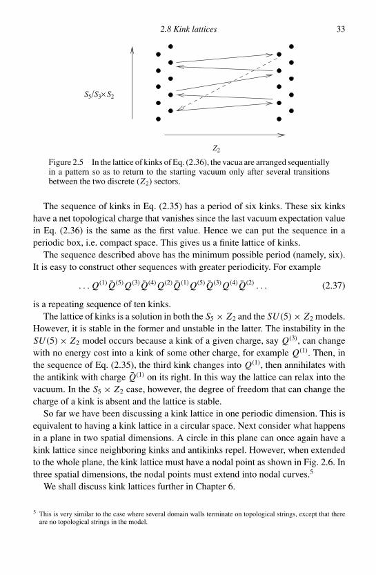
2.8 Kink lattices 33
Z2
S5/S3× S2
Figure 2.5 In the lattice of kinks of Eq. (2.36), the vacua are arranged sequentiallyin a pattern so as to return to the starting vacuum only after several transitionsbetween the two discrete (Z2) sectors.
The sequence of kinks in Eq. (2.35) has a period of six kinks. These six kinkshave a net topological charge that vanishes since the last vacuum expectation valuein Eq. (2.36) is the same as the first value. Hence we can put the sequence in aperiodic box, i.e. compact space. This gives us a finite lattice of kinks.
The sequence described above has the minimum possible period (namely, six).It is easy to construct other sequences with greater periodicity. For example
. . . Q(1) Q(5) Q(3) Q(4) Q(2) Q(1) Q(5) Q(3) Q(4) Q(2) . . . (2.37)
is a repeating sequence of ten kinks.The lattice of kinks is a solution in both the S5 × Z2 and the SU (5) × Z2 models.
However, it is stable in the former and unstable in the latter. The instability in theSU (5) × Z2 model occurs because a kink of a given charge, say Q(3), can changewith no energy cost into a kink of some other charge, for example Q(1). Then, inthe sequence of Eq. (2.35), the third kink changes into Q(1), then annihilates withthe antikink with charge Q(1) on its right. In this way the lattice can relax into thevacuum. In the S5 × Z2 case, however, the degree of freedom that can change thecharge of a kink is absent and the lattice is stable.
So far we have been discussing a kink lattice in one periodic dimension. This isequivalent to having a kink lattice in a circular space. Next consider what happensin a plane in two spatial dimensions. A circle in this plane can once again have akink lattice since neighboring kinks and antikinks repel. However, when extendedto the whole plane, the kink lattice must have a nodal point as shown in Fig. 2.6. Inthree spatial dimensions, the nodal points must extend into nodal curves.5
We shall discuss kink lattices further in Chapter 6.
5 This is very similar to the case where several domain walls terminate on topological strings, except that thereare no topological strings in the model.
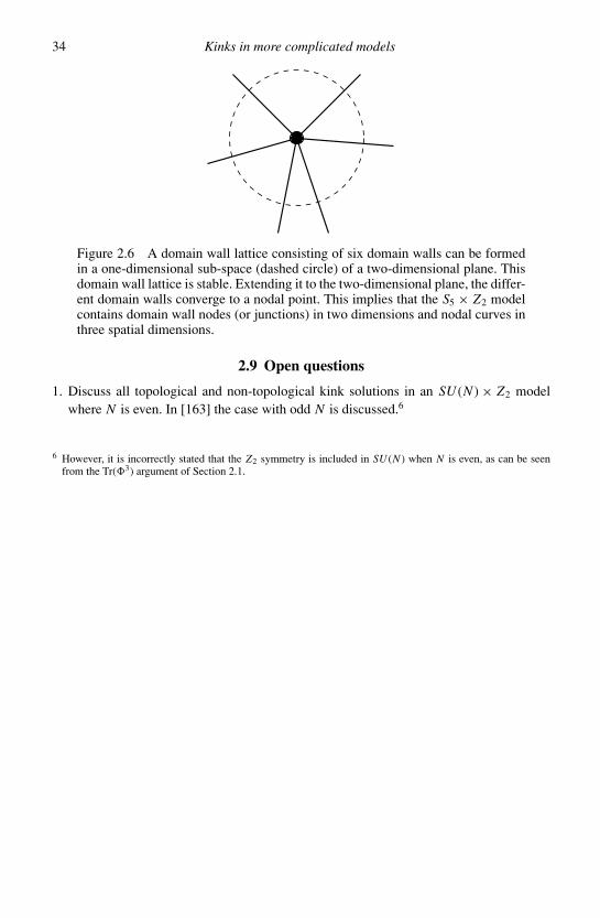
34 Kinks in more complicated models
Figure 2.6 A domain wall lattice consisting of six domain walls can be formedin a one-dimensional sub-space (dashed circle) of a two-dimensional plane. Thisdomain wall lattice is stable. Extending it to the two-dimensional plane, the differ-ent domain walls converge to a nodal point. This implies that the S5 × Z2 modelcontains domain wall nodes (or junctions) in two dimensions and nodal curves inthree spatial dimensions.
2.9 Open questions
1. Discuss all topological and non-topological kink solutions in an SU (N ) × Z2 modelwhere N is even. In [163] the case with odd N is discussed.6
6 However, it is incorrectly stated that the Z2 symmetry is included in SU (N ) when N is even, as can be seenfrom the Tr(3) argument of Section 2.1.

3
Interactions
In the previous two chapters, we have described kink solutions in several modelsbut these solutions have mostly been discussed in isolation. In any real system, thereis a variety of kinks and antikinks, in addition to small excitations (particles) of thefields. The interactions of kinks with other kinks and with particles play an importantrole in the evolution of the system. The motion of kinks is also accompanied bythe radiation of particles. Ambient particles in the system scatter off kinks, andkinks collide with each other, and perhaps annihilate into particles. As discussedin Section 1.9, in some models a kink-antikink pair can bind together to form anon-dissipative solution which is called a “breather.” In other models, approximatebreather solutions have been found, which play an important role in the scatteringof a kink and an antikink. These topics are discussed in the following sections.
3.1 Breathers and oscillons
So far we have been considering kinks, which are static solutions to the equationsof motion. In the sine-Gordon model of Eq. (1.51), a one-parameter family of non-static, dissipationless solutions is also known. These are bound states of a kink andan antikink and are called breathers. The breather solution was described briefly inSection 1.9 and can be re written as
φb(t, x ; v) = 4
βtan−1
[sin(v
√αt/
√1 + v2)
v cosh(√
αx/√
1 + v2)
](3.1)
where v is a free parameter (see Fig. 3.1). We will have more to say about breatherswhen we quantize kinks in Chapter 4 as they play a very fundamental role in thenovel duality between the sine-Gordon model and the massive Thirring model (seeSection 4.7).
Breather solutions are not known to exist in the λφ4 model [135]. However,numerical studies of the scattering of a Z2 kink and antikink revealed the existence of
35
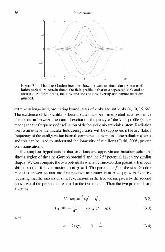
36 Interactions
−10 −5 0 5 10−1
−0.5
0
0.5
1
Figure 3.1 The sine-Gordon breather shown at various times during one oscil-lation period. At certain times, the field profile is that of a separated kink and anantikink. At other times, the kink and the antikink overlap and cannot be distin-guished.
extremely long-lived, oscillating bound states of kinks and antikinks [4, 19, 26, 64].The existence of kink-antikink bound states has been interpreted as a resonancephenomenon between the natural excitation frequency of the kink profile (shapemode) and the frequency of oscillation of the bound kink-antikink system. Radiationfrom a time-dependent scalar field configuration will be suppressed if the oscillationfrequency of the configuration is small compared to the mass of the radiation quantaand this can be used to understand the longevity of oscillons (Farhi, 2005, privatecommunication).
The simplest hypothesis is that oscillons are approximate breather solutionssince a region of the sine-Gordon potential and the λφ4 potential have very similarshapes. We can compare the two potentials when the sine-Gordon potential has beenshifted so that it has a maximum at φ = 0. The parameter β in the sine-Gordonmodel is chosen so that the first positive minimum is at φ = +η. α is fixed byrequiring that the masses of small excitations in the true vacua, given by the secondderivative of the potential, are equal in the two models. Then the two potentials aregiven by
VZ2 (φ) = λ
4(φ2 − η2)2 (3.2)
VsG() = α
β2(1 − cos(β(φ − η))) (3.3)
with
α = 2λη2, β = π
η(3.4)
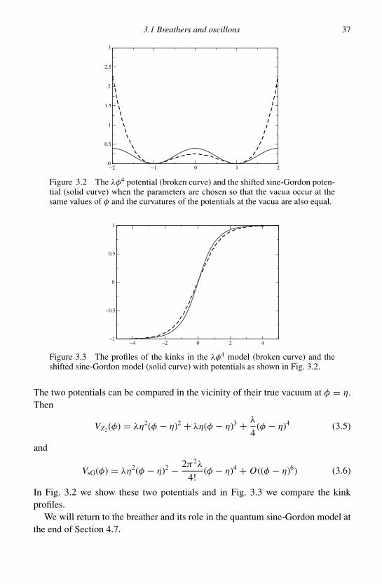
3.1 Breathers and oscillons 37
−2 −1 0 1 20
0.5
1
1.5
2
2.5
3
Figure 3.2 The λφ4 potential (broken curve) and the shifted sine-Gordon poten-tial (solid curve) when the parameters are chosen so that the vacua occur at thesame values of φ and the curvatures of the potentials at the vacua are also equal.
−4 −2 0 2 4−1
−0.5
0
0.5
1
Figure 3.3 The profiles of the kinks in the λφ4 model (broken curve) and theshifted sine-Gordon model (solid curve) with potentials as shown in Fig. 3.2.
The two potentials can be compared in the vicinity of their true vacuum at φ = η.Then
VZ2 (φ) = λη2(φ − η)2 + λη(φ − η)3 + λ
4(φ − η)4 (3.5)
and
VsG(φ) = λη2(φ − η)2 − 2π2λ
4!(φ − η)4 + O((φ − η)6) (3.6)
In Fig. 3.2 we show these two potentials and in Fig. 3.3 we compare the kinkprofiles.
We will return to the breather and its role in the quantum sine-Gordon model atthe end of Section 4.7.
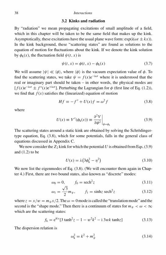
38 Interactions
3.2 Kinks and radiation
By “radiation” we mean propagating excitations of small amplitude of a field,which in this chapter will be taken to be the same field that makes up the kink.Asymptotically, these excitations have the usual plane wave form: exp(i(ωt ± kx)).In the kink background, these “scattering states” are found as solutions to theequation of motion for fluctuations about the kink. If we denote the kink solutionby φk(x), the fluctuation field ψ(t, x) is
ψ(t, x) = φ(t, x) − φk(x) (3.7)
We will assume |ψ | 〈φ〉, where 〈φ〉 is the vacuum expectation value of φ. Tofind the scattering states, we take ψ = f (x)e−iωt where it is understood that thereal or imaginary part should be taken – in other words, the physical modes are[ f (x)e−iωt ± f ∗(x)e+iωt ]. Perturbing the Lagrangian for φ (first line of Eq. (1.2)),we find that f (x) satisfies the (linearized) equation of motion
H f ≡ − f ′′ + U (x) f = ω2 f (3.8)
where
U (x) ≡ V ′′(φk(x)) ≡ ∂2V
∂φ2
∣∣∣∣φ=φk
(3.9)
The scattering states around a static kink are obtained by solving the Schrodinger-type equation, Eq. (3.8), which for some potentials, falls in the general class ofequations discussed in Appendix C.
We now consider the Z2 kink for which the potential U is obtained from Eqs. (3.9)and (1.2) to be
U (x) = λ(3φ2
k − η2)
(3.10)
We now list the eigenmodes of Eq. (3.8). (We will encounter them again in Chap-ter 4.) First, there are two bound states, also known as “discrete” modes:
ω0 = 0, f0 = sech2z (3.11)
ω1 =√
3
2mψ, f1 = sinhz sech2z (3.12)
where z = x/w = mψ x/2. The ω = 0 mode is called the “translation mode” and thesecond is the “shape mode.” Then there is a continuum of states for mψ < ω < ∞which are the scattering states:
fk = eikx [3 tanh2z − 1 − w2k2 − i 3wk tanhz] (3.13)
The dispersion relation is
ω2k = k2 + m2
ψ (3.14)

3.3 Structure of the fluctuation Hamiltonian 39
We are now interested in processes that involve both a kink and the scatteringstates (radiation). For example, if a kink accelerates, it will emit radiation. Whatis the radiated power? The answer will depend on the forces that make the kinkaccelerate and whether or not these forces deform the structure of the kink.1 Weshall examine the radiation from kink shape deformations and other interactions ofkinks and radiation after a brief diversion in the next section.
3.3 Structure of the fluctuation Hamiltonian
In this section we will show two interesting properties of the fluctuationHamiltonian, H , defined in Eq. (3.8). The first is that the potential U (x) has avery special form that implies that the Hamiltonian can be factored. The second isthat there exists a “partner Hamiltonian” with (almost) the same spectrum as theoriginal Hamiltonian.
The special form of U follows from the fact that the kink has a translation zeromode (see Section 1.1). Hence there exists an eigenstate with ω = 0. Denote this“translation mode” by ψt. Hence
Hψt = (−∂2 + U (x))ψt = 0 (3.15)
Therefore
U (x) = ψ ′′t
ψt(3.16)
which can also be rewritten as
U (x) = f ′ + f 2, f = (ln(ψt))′ (3.17)
For the particular cases of the Z2 and sine-Gordon kinks, not only is U (x)of the form in Eq. (3.17) but it is also reflectionless. Then, an incident wave isfully transmitted and the reflection coefficient vanishes. In this case, the only non-trivial characteristic of scattering states is that the waves get a phase shift owing tothe presence of U (x). This property will be useful when we quantize the kink inSection 4.1.
The Hamiltonian H with a potential of the form in Eq. (3.17) has the importantproperty that it can be factored
H = A+ A ≡ (+∂ + f )(−∂ + f ) (3.18)
Therefore the equation for the eigenstates is simply
H f = A+ A f = ω2 f (3.19)
1 In the case of domain walls in three spatial dimensions, the curvature of the wall is itself responsible foracceleration. This motion leads to the emission of scalar and gravitational radiation and will be discussed inChapter 8.
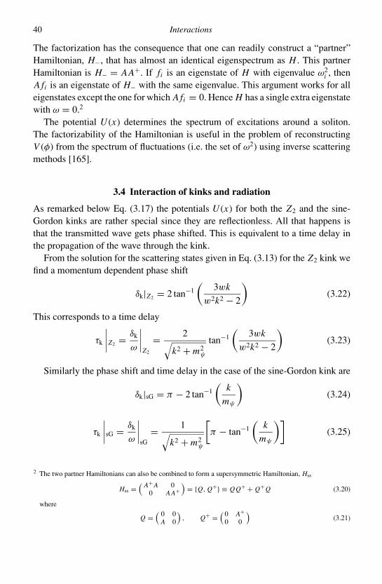
40 Interactions
The factorization has the consequence that one can readily construct a “partner”Hamiltonian, H−, that has almost an identical eigenspectrum as H . This partnerHamiltonian is H− = AA+. If fi is an eigenstate of H with eigenvalue ω2
i , thenA fi is an eigenstate of H− with the same eigenvalue. This argument works for alleigenstates except the one for which A fi = 0. Hence H has a single extra eigenstatewith ω = 0.2
The potential U (x) determines the spectrum of excitations around a soliton.The factorizability of the Hamiltonian is useful in the problem of reconstructingV (φ) from the spectrum of fluctuations (i.e. the set of ω2) using inverse scatteringmethods [165].
3.4 Interaction of kinks and radiation
As remarked below Eq. (3.17) the potentials U (x) for both the Z2 and the sine-Gordon kinks are rather special since they are reflectionless. All that happens isthat the transmitted wave gets phase shifted. This is equivalent to a time delay inthe propagation of the wave through the kink.
From the solution for the scattering states given in Eq. (3.13) for the Z2 kink wefind a momentum dependent phase shift
δk|Z2 = 2 tan−1
(3wk
w2k2 − 2
)(3.22)
This corresponds to a time delay
τk
∣∣∣∣Z2 = δk
ω
∣∣∣∣Z2
= 2√k2 + m2
ψ
tan−1
(3wk
w2k2 − 2
)(3.23)
Similarly the phase shift and time delay in the case of the sine-Gordon kink are
δk|sG = π − 2 tan−1
(k
mψ
)(3.24)
τk
∣∣∣∣sG = δk
ω
∣∣∣∣sG
= 1√k2 + m2
ψ
[π − tan−1
(k
mψ
)](3.25)
2 The two partner Hamiltonians can also be combined to form a supersymmetric Hamiltonian, Hss
Hss =( A+ A 0
0 AA+)
= Q, Q+ ≡ Q Q+ + Q+ Q (3.20)
where
Q =( 0 0
A 0
), Q+ =
( 0 A+0 0
)(3.21)
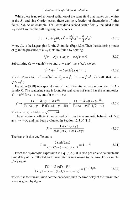
3.4 Interaction of kinks and radiation 41
While there is no reflection of radiation of the same field that makes up the kinkin the Z2 and sine-Gordon cases, there can be reflection of fluctuations of otherfields [53]. As an example [171], consider a second scalar field χ included in theZ2 model so that the full Lagrangian becomes
L = Lφ + 1
2(∂µχ )2 − m2
χ
2χ2 − σ
2φ2χ2 (3.26)
where Lφ is the Lagrangian for the Z2 model (Eq. (1.2)). Then the scattering modesof χ in the presence of a Z2 kink are found by solving
∂2t χ − ∂2
x χ + m2χχ + σφ2
kχ = 0 (3.27)
Substituting φk = η tanh(x/w) and χ = exp(−iωt) f (x), we get
∂2X f + (ν2 − σ sech2(X )) f = 0 (3.28)
where X ≡ x/w, ν2 = w2(ω2 − m2χ − ση2), σ = ση2w2. (Recall that w =√
2/λη2.)Equation (3.28) is a special case of the differential equation described in Ap-
pendix C. The scattering state is found for real values of ν and has the asymptotics:f → eikx for x → ∞, and for x → −∞:
f → (1 − ikw)(−ik)eikx
(1/2 + γ − ik)(1/2 − γ − ik)+ (1 − ikw)(ik)e−ikx
(1/2 + γ )(1/2 − γ )(3.29)
where k = ν/w and γ = √σ + 1/4.
The reflection coefficient can be read off from the asymptotic behavior of f (x)as x → −∞ and has been evaluated in Section 12.3 of [113]
R = 1 + cos(2πγ )
cosh(2πk) + cos(2πγ )(3.30)
The transmission coefficient is
T = 2 sinh2(πk)
cosh(2πk) + cos(2πγ )= 1 − R (3.31)
From the asymptotic expression in Eq. (3.29), it is also possible to calculate thetime delay of the reflected and transmitted waves owing to the kink. For example,if we write
(1 − ikw)(−ik)
(1/2 + γ − ik)(1/2 − γ − ik)= |T |1/2eiδk (3.32)
where T is the transmission coefficient above, then the time delay of the transmittedwave is given by δk/ω.
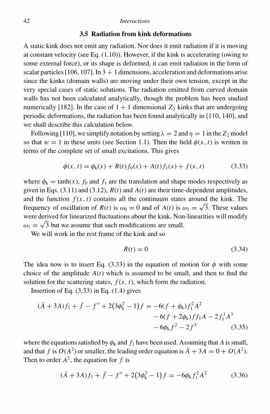
42 Interactions
3.5 Radiation from kink deformations
A static kink does not emit any radiation. Nor does it emit radiation if it is movingat constant velocity (see Eq. (1.10)). However, if the kink is accelerating (owing tosome external force), or its shape is deformed, it can emit radiation in the form ofscalar particles [106, 107]. In 3 + 1 dimensions, acceleration and deformations arisesince the kinks (domain walls) are moving under their own tension, except in thevery special cases of static solutions. The radiation emitted from curved domainwalls has not been calculated analytically, though the problem has been studiednumerically [182]. In the case of 1 + 1 dimensional Z2 kinks that are undergoingperiodic deformations, the radiation has been found analytically in [110, 140], andwe shall describe this calculation below.
Following [110], we simplify notation by setting λ = 2 and η = 1 in the Z2 modelso that w = 1 in these units (see Section 1.1). Then the field φ(x, t) is written interms of the complete set of small excitations. This gives
φ(x, t) = φk(x) + R(t) f0(x) + A(t) f1(x) + f (x, t) (3.33)
where φk = tanh(x), f0 and f1 are the translation and shape modes respectively asgiven in Eqs. (3.11) and (3.12), R(t) and A(t) are their time-dependent amplitudes,and the function f (x, t) contains all the continuum states around the kink. Thefrequency of oscillation of R(t) is ω0 = 0 and of A(t) is ω1 = √
3. These valueswere derived for linearized fluctuations about the kink. Non-linearities will modifyω1 = √
3 but we assume that such modifications are small.We will work in the rest frame of the kink and so
R(t) = 0 (3.34)
The idea now is to insert Eq. (3.33) in the equation of motion for φ with somechoice of the amplitude A(t) which is assumed to be small, and then to find thesolution for the scattering states, f (x, t), which form the radiation.
Insertion of Eq. (3.33) in Eq. (1.4) gives
( A + 3A) f1 + f − f ′′ + 2(3φ2
k − 1)
f = −6( f + φk) f 21 A2
− 6( f + 2φk) f f1 A − 2 f 31 A3
− 6φk f 2 − 2 f 3 (3.35)
where the equations satisfied by φk and f1 have been used. Assuming that A is small,and that f is O(A2) or smaller, the leading order equation is A + 3A = 0 + O(A2).Then to order A2, the equation for f is
( A + 3A) f1 + f − f ′′ + 2(3φ2
k − 1)
f = −6φk f 21 A2 (3.36)
3.5 Radiation from kink deformations 43
The f -independent terms on the right-hand side of Eq. (3.35) are source termswhich cause radiation. Hence f will not be zero at order A2. The terms will alsocause the amplitude, A, of the shape mode to depart from the purely oscillatorybehavior. To determine how much of the source affects radiation and how muchaffects the shape mode, note that f1 and f are orthogonal∫
dx f1(x) f (x, t) = 0 (3.37)
So we can decompose the equation into a direction parallel to f1 in mode space andorthogonal to it. One assumption we have to make is that the back-reaction of theradiative modes on the shape mode is higher order in A. For example, Eq. (3.37)does not by itself imply that f ′′ and f1 are orthogonal. Then, multiplying Eq. (3.36)by f1 and integrating over all space gives
A + 3A = −6A2∫
dxφk f 21 ≡ −6αA2 (3.38)
provided we have normalized f1 so that∫dx[ f1(x)]2 = 1 (3.39)
Explicit evaluation gives
α = 3π
32(3.40)
The equation orthogonal to f1 is
f − f ′′ + 2(3φ2
k − 1)
f = −6φk f 21 A2 + 6α f1 A2 (3.41)
and this will determine the radiation from the deformed kink once we have specifiedA.
The leading order solution for A is
A = A0 cos(√
3t) (3.42)
Hence
A2 = A20
2[cos(2
√3t) + 1] (3.43)
This form implies that the source for f in Eq. (3.41) has a time-dependent pieceand another time-independent piece. Since the equation is linear in f , only thetime-dependent piece proportional to cos(2
√3t) is important. Setting
f (x, t) = Re(eiωt F(x)) (3.44)
44 Interactions
the equation that needs to be solved is
−F ′′ + (6φ2k − 2 − ω2
)F = 3
2
(α f1 − φk f 2
1
)A2
0ei(ω0−ω)t (3.45)
where ω0 = 2√
3. Since the left-hand side is time-independent, this only has solu-tions for
ω = ω0 = 2√
3 (3.46)
and then all the solutions of the homogeneous equation are known (see Appendix C;[113, 126]). The solutions of the homogeneous equation with plane wave asymp-totics are
Fq(x) = (3φ2k − 1 − q2 − 3iqφk
)eiqx (3.47)
where q = √ω2 − 4. Knowing all the solutions of the homogeneous equation, it is
possible to explicitly construct the (retarded) Green’s function suitable for outgoingradiation.
G(x, y) =−F−q(y)Fq(x)/W, (x < y)
−Fq(y)F−q(x)/W, (x > y)(3.48)
where W is the Wronskian
W = Fq(x)F−q′(x) − Fq
′(x)F−q(x) (3.49)
The Wronskian is a constant and its value can be found by using the explicit solutions
W = −2iq(q2 + 1)(q2 + 4) (3.50)
The solution of the inhomogeneous equation (3.45) is found by convoluting thesource with the Green’s function
F(x) =∫ +∞
−∞dy G(x, y)
3
2
[α f1(y) − φk(y) f 2
1 (y)]A2
0 (3.51)
With a little more manipulation, we obtain the radiation field in the x → +∞ limit
f (x, t) = Re
[ −3A20ei(ωt−qx)
2iq(2 − q2 − 3iq)
∫ +∞
−∞dy φk(y) f 2
1 (y)Fq(y)
](3.52)
with ω = ω0 = 2√
3 and q = √ω2 − 4 = 2
√2. The integral can be done explicitly
leading to
f (x, t) = πq(q2 − 2)
32 sinh(πq/2)
√q2 + 4
q2 + 1A2
0 cos(ωt − qx − δ) (3.53)
3.7 Scattering of kinks 45
The phase δ can be read off from Eq. (3.52) because the integral is purely imaginaryand does not contribute
δ = tan−1
(3q
q2 − 2
)(3.54)
Now that we have the solution for the radiation field, we can find the energyflux by using the T0i components of the energy-momentum tensor in Eq. (1.39).Including a factor of 2 to account for the radiation toward x → −∞, we obtain theradiated power [110]
dE
dt= −0.020A4
0 (3.55)
The back-reaction of the radiation on the deformation amplitude can be estimatedon the grounds of energy conservation. In [110] the results above are compared tothe results of a numerical evolution of the deformations using the full non-linearequations with good agreement.
3.6 Kinks from radiation
By time reversing kink and antikink annihilation, it should be possible to obtainkink-antikink creation from incoming radiation. However, the stream of incomingradiation would have to be sent with just the correct phase relationship and energy.Such initial conditions occupy zero volume in the space of all initial conditions. Amore physical problem is to identify the set, or a large subset, of initial conditionsfor the incoming radiation that will lead to kink-antikink creation. This problem isunsolved. Yet certain interesting results have been obtained in [110] in the “gradientflow” approximation in which the second time derivative terms in the equation ofmotion are neglected.
Consider the collision of two kinks in the presence of a pre-existing kink [110],as depicted in Fig. 3.4. As the kink-antikink-kink (kkk) system evolves, a kink-antikink annihilate, and we are left with a kink whose shape is excited. Reversingthis process, if we start with a kink whose shape is excited, it can produce a kink-antikink pair. In [110], this relation between the shape mode and the creation of akink-antikink pair was explored.
3.7 Scattering of kinks
The sine-Gordon model is a famous example of a completely integrable system [48].Sine-Gordon kinks are examples of “solitons” in the strict mathematical sense inwhich when two or more solitons (or anti-solitons) scatter, they simply pass through
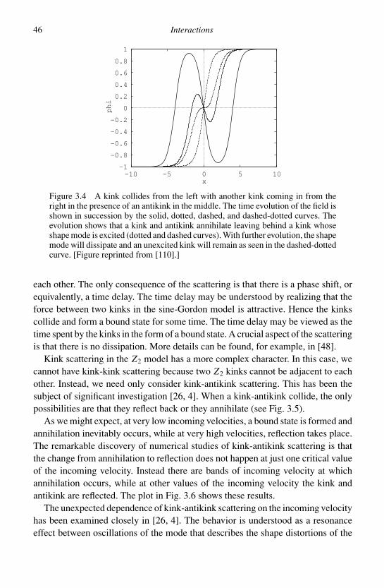
46 Interactions
-1
-0.8
-0.6
-0.4
-0.2
0
0.2
0.4
0.6
0.8
1
-10 -5 0 5 10
ph
i
x
Figure 3.4 A kink collides from the left with another kink coming in from theright in the presence of an antikink in the middle. The time evolution of the field isshown in succession by the solid, dotted, dashed, and dashed-dotted curves. Theevolution shows that a kink and antikink annihilate leaving behind a kink whoseshape mode is excited (dotted and dashed curves). With further evolution, the shapemode will dissipate and an unexcited kink will remain as seen in the dashed-dottedcurve. [Figure reprinted from [110].]
each other. The only consequence of the scattering is that there is a phase shift, orequivalently, a time delay. The time delay may be understood by realizing that theforce between two kinks in the sine-Gordon model is attractive. Hence the kinkscollide and form a bound state for some time. The time delay may be viewed as thetime spent by the kinks in the form of a bound state. A crucial aspect of the scatteringis that there is no dissipation. More details can be found, for example, in [48].
Kink scattering in the Z2 model has a more complex character. In this case, wecannot have kink-kink scattering because two Z2 kinks cannot be adjacent to eachother. Instead, we need only consider kink-antikink scattering. This has been thesubject of significant investigation [26, 4]. When a kink-antikink collide, the onlypossibilities are that they reflect back or they annihilate (see Fig. 3.5).
As we might expect, at very low incoming velocities, a bound state is formed andannihilation inevitably occurs, while at very high velocities, reflection takes place.The remarkable discovery of numerical studies of kink-antikink scattering is thatthe change from annihilation to reflection does not happen at just one critical valueof the incoming velocity. Instead there are bands of incoming velocity at whichannihilation occurs, while at other values of the incoming velocity the kink andantikink are reflected. The plot in Fig. 3.6 shows these results.
The unexpected dependence of kink-antikink scattering on the incoming velocityhas been examined closely in [26, 4]. The behavior is understood as a resonanceeffect between oscillations of the mode that describes the shape distortions of the
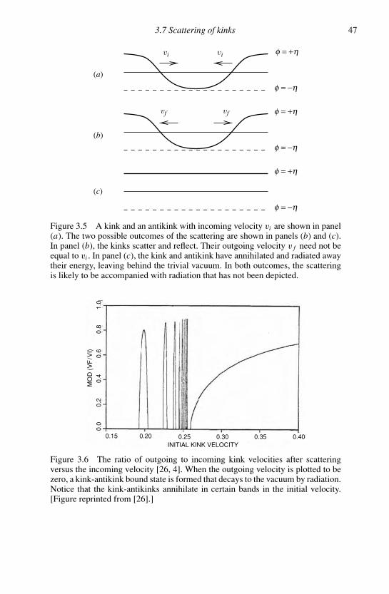
3.7 Scattering of kinks 47
(c)
f = +h
f = +h
f = +h
f = −h
f = −h
f = −h
(a)
(b)
vivi
vf vf
Figure 3.5 A kink and an antikink with incoming velocity vi are shown in panel(a). The two possible outcomes of the scattering are shown in panels (b) and (c).In panel (b), the kinks scatter and reflect. Their outgoing velocity v f need not beequal to vi . In panel (c), the kink and antikink have annihilated and radiated awaytheir energy, leaving behind the trivial vacuum. In both outcomes, the scatteringis likely to be accompanied with radiation that has not been depicted.
0.15
0.0
0.2
0.4
0.6
0.8
1.0
0.20 0.25INITIAL KINK VELOCITY
0.30 0.35 0.40
MO
D (
VF
/VI)
Figure 3.6 The ratio of outgoing to incoming kink velocities after scatteringversus the incoming velocity [26, 4]. When the outgoing velocity is plotted to bezero, a kink-antikink bound state is formed that decays to the vacuum by radiation.Notice that the kink-antikinks annihilate in certain bands in the initial velocity.[Figure reprinted from [26].]

48 Interactions
Figure 3.7 Two curved domain walls collide and intercommute. At the collisionpoint, there is lots of radiation owing to annihilation or owing to the formation ofa closed domain wall that then collapses and decays into radiation. To imagine thewalls in three dimensions, rotate the figures along the horizontal axis. In the initialstate the two curved walls are disconnected from each other while in the final state,the wall is in the shape of a “wormhole,” with a sphere in the middle.
kinks and the oscillations of the kinks as a whole owing to kink-antikink interactions.We shall not describe the details of the analysis here.
The scattering of SU (5) × Z2 kinks has been studied numerically in [121]. Inthis case, there is an additional degree of freedom, namely the non-Abelian chargeof the colliding kinks (or “color”) and there are a variety of initial conditions that canbe considered. For the stable variety of kinks – the q = 2 kinks (see Section 3.2) –the scattering of kinks and antikinks of the same color is qualitatively similar to thatof Z2 kinks. If the colors are different, however, there is a repulsive force betweenthe kinks and they are observed to bounce back elastically.
3.8 Intercommuting of domain walls
We finally consider the collision of two domain walls. The outcome is found bynumerical evolution of the equations of motion. As the walls come together, theyreconnect along the curve of intersection [136] as shown in Fig. 3.7. This processis called “intercommuting” or, simply, “reconnection.”
3.9 Open questions
1. Suppose we want to create a well-separated Z2 kink-antikink pair by colliding smallamplitude plane waves (particles) in the φ = +η vacuum. What conditions must beimposed on the incoming waves? What is the space of initial conditions that leads todomain wall formation? Can the initial conditions be implemented in a practical setting(e.g. accelerator experiments)?
2. Can a domain wall lattice be generalized to other defects, e.g. a lattice of strings andmonopoles?

3.9 Open questions 49
3. Study the interaction of domain walls and strings/magnetic monopoles in a model thatcontains both types of defects e.g. the SU (5) × Z2 model has walls and magneticmonopoles.
4. Construct a sine-Gordon-like breather field configuration in the λφ4 model. This will notbe an exact solution of the field equation of motion. Hence it will radiate. Calculate theradiated power. Are there circumstances in which the radiated power is very small?
5. Can the analysis of radiation from kink deformations be extended to the case of oscillatingdomain walls? The simplest procedure would be to decompose the field as in Eq. (3.33)and to include a suitable external (harmonic) potential that drives the translation modeonly. This will cause the kink to oscillate as a whole without deformations. However, theoscillations will source the shape mode and the radiation, and an analysis of the kind inSection 3.5 seems feasible.
6. Can the analysis of radiation from kink deformations be extended to the case of sphericaldomain walls?
7. How can the radiation analysis be extended to vortex solutions in two or more spatialdimensions?
4
Kinks in quantum field theory
A particle in a classical harmonic oscillator potential, mω2x2/2, has minimum en-ergy when it sits at rest at the bottom of the potential. Then the particle’s energyvanishes. The Heisenberg uncertainty principle however modifies this picture forthe quantum harmonic oscillator. The particle cannot sit at rest (with definite mo-mentum) at the bottom of the potential (a definite location). Indeed, the quantumzero point motion lifts the ground state energy to ω/2. Further, the excited statesof the simple harmonic oscillator are discrete and occur at energies (n + 1/2)ω,n = 0, 1, 2, . . .
Just as the classical harmonic oscillator is modified by quantum effects, anyclassical solution to a field theory is also modified by quantum effects. Quantumeffects give corrections to the classical kink energy owing to zero point quantumfield fluctuations. These quantum corrections are small provided the coupling con-stant in the model is weak. To “quantize the kink” means to evaluate all the energylevels of the kink (first quantization) and to develop a framework for doing quantumfield theory in a kink background. This involves identifying all excitations in thepresence of the kink and their interactions. The field theory of the excitations inthe non-trivial background of the kink is akin to second quantization. Finally, onewould also like to describe the creation and annihilation of kinks themselves bysuitable kink creation and annihilation operators. This would be the elusive thirdquantization.
Initially we calculate the leading order quantum corrections to the energy of theZ2 and sine-Gordon kinks. As these two examples illustrate, the precise value ofthe quantum correction depends on the exact model and kink under consideration.Yet there is one common feature – quantum corrections tend to reduce the energyof the kink. This result is quite general and we prove it using a variational argumentin Section 4.5.
The quantum corrections to the kink mass are obtained by using a perturbativeanalysis where the coupling constant is the expansion parameter, as first done
50
4.1 Quantization of kinks: broad outline 51
in [38, 42]. For fixed values of the masses of particles in the field theory, theenergy of the classical solution is proportional to the coupling constant raised toa negative power (for example, see Eq. (1.20)) and so the perturbative analysisholds only if the kink is much more massive than the particles in the model. As thecoupling constant is increased, quantum effects become stronger and eventuallythe perturbative scheme breaks down. Remarkably, the sine-Gordon model is stillamenable to analysis in this regime and, at strong coupling, the sine-Gordon kinksbecome lighter than the particles. Indeed, there exists a weakly coupled descriptionof the model in which perturbative methods can be used: this is the massive Thirringmodel in which the particles (low energy excitations of a fermionic field) correspondto the sine-Gordon kinks at strong coupling (see Section 4.7).
The phenomenon observed in the sine-Gordon and massive Thirring models, inwhich solitons of one model (Model 1) are identified with the particles of a secondmodel (Model 2) and vice versa in certain regimes of the coupling constants, isknown as “duality.” Model 1 is said to be dual to Model 2 if the particle-plus-solitonspectrum of Model 1 maps onto the soliton-plus-particle spectrum of Model 2 andvice versa. Both models describe the same physics, except that the light and heavydegrees of freedom are interchanged.
The Z2 model does not share the remarkable symmetries of the sine-Gordonmodel and less is known about the Z2 kink at strong coupling. However, the massof the Z2 kink can be evaluated at strong coupling using lattice field theory. Wedescribe these results in Section 4.8 and conclude, once again, that the kink becomesless massive as the coupling is increased and eventually becomes massless.
In this book, we only describe quantization of the mass of the kink using canonicaltechniques. A more extensive discussion of various other techniques and issues canbe found in [35, 126] and in the series of papers in [38, 42].
4.1 Quantization of kinks: broad outline
In this section, we evaluate the contribution of the zero point fluctuations to theenergy of the kink. Then we briefly discuss excited states.
The quantization procedure can be outlined as follows:
Consider a field theory in two dimensions with compact spatial dimension of sizeL , assumed large compared to any other length scale in the problem. Periodicboundary conditions are imposed on the fields. Eventually take L → ∞.
Consider small quantum fluctuations, ψ , about the classical kink background,φk,
φ(t, x) = φk(x) + ψ(t, x) (4.1)

52 Kinks in quantum field theory
n = 0n = ± 1
n = ± 2
n = ± 2
n = −1n = +1n = 0
Figure 4.1 A trivial potential on a periodic space with period L is shown on theleft. The field modes are labeled by an integer n = 0, ±1, ±2, . . . When there is akink, the potential felt by the modes becomes non-trivial as depicted by the curvedbottom of the figure on the right. What used to be the n = 0 mode in the trivialpotential (on the left) becomes the lowest bound state, the zero mode, in the non-trivial potential. Similarly a linear combination of the n = ±1 modes in the trivialbox may become a second bound state (n = +1 in this illustration) and the otherstates remain unbound but shift in form and energy.
Linearize the equation for ψ and then quantize, that is, regard the field ψ as aquantum operator
ψ(t, x) =∑
[ak fk(t, x) + a†k f ∗
k (t, x)] (4.2)
where a†k and ak are creation and annihilation operators. The fk are mode functions
i.e. orthonormal solutions of the linearized equations of motion for ψ in the kinkbackground. The equation satisfied by fk is
∂2t fk − ∂2
x fk + V ′′(φk(x)) fk = 0 (4.3)
Find all the eigenmodes, fk, of the fluctuations and their eigenfrequencies ωk. Asshown in Fig. 4.1, in the presence of the kink the modes are displaced. Some ofthe low-lying modes without the kink become bound states in the presence of thekink, and the others become scattering states as L → ∞.
Each eigenmode corresponds to a quantum harmonic oscillator with zero pointfluctuations. Sum up the zero point energies of all the modes to get the quantumcorrection to the classical kink energy, Ecl,
E = Ecl +∑
i
1
2ωi (4.4)
In the L → ∞ limit, the sum over the modes becomes a sum over bound statesand an integral over scattering states. Also note that Eq. (4.4) is only valid toleading order in the quantum corrections since we have ignored interactions of thefluctuation field, ψ .
4.1 Quantization of kinks: broad outline 53
In following this procedure, quantum field theoretic subtleties arise.
The zero point energy of the trivial vacuum (without the kink) must be subtractedfrom the zero point energy of the kink since we want to define the energy of thetrivial vacuum to be zero. Therefore
E = Ecl +∑
i
1
2ωi −
[Ecl,0 +
∑i
1
2ω
(0)i
]
where Ecl,0 is the classical energy of the trivial vacuum and is chosen to vanish(Ecl,0 = 0), and ω
(0)i are the eigenfrequencies of the modes in the trivial vacuum.
The energy must be expressed in terms of renormalized parameters.
In the trivial vacuum, the energy eigenvalue for the mode with n nodes is
ω(0)n =
√k2
n + m2ψ (4.5)
where kn = 2πn/L and n ∈ Z, the set of all integers. Now suppose that the kinkpotential V ′′ is turned on slowly, i.e. that the potential term in Eq. (4.3) is multipliedby a parameter that vanishes for the free field theory and is continuously increasedto one to get to the kink case. As the parameter increases, modes in the trivialbox evolve into modes in the kink background. Some of the low-lying modes inthe trivial box become the bound states of the kink. Let us label these modes bythe index b (for “bound”) and the remaining modes by c (for “continuum”). (In theexample of Fig. 4.1, b = 0, 1, and c is any integer except for 0, 1.) Then
E = Ecl + 1
2
∑b
(ωb − ω
(0)b
)+ 1
2
∑c
[√p2
c + m2ψ −
√k2
c + m2ψ
](4.6)
where ωc ≡√
p2c + m2
ψ and mψ denotes the mass of the ψ particles. In the limit
L → ∞, the sum over continuum states becomes an integral.The terms in Eq. (4.6) can be understood quite simply. The first term on the right
is the classical kink energy, the second contains the excess quantum correctionsowing to the zero point motion of the modes bound to the kink, and the third termis the excess energy in the zero point motion of the modes that are not bound to thekink. The wave numbers of the scattering modes in the background of the kink aredenoted by pν while that of the modes in the trivial vacuum by kn .
In the trivial vacuum and when L → ∞, the scattering states are plane waves,which are both energy and momentum eigenstates with kn = 2πn/L . In the pres-ence of the kink, the scattering states are energy eigenstates but not momentumeigenstates and, in general, an incoming wave gets both reflected and transmit-ted. Without specifying the field theory, further progress is possible when thescattering potential, V ′′(φk(x)), is reflectionless. This may seem very restrictive,but it holds for both the Z2 and sine-Gordon models and we assume it to be
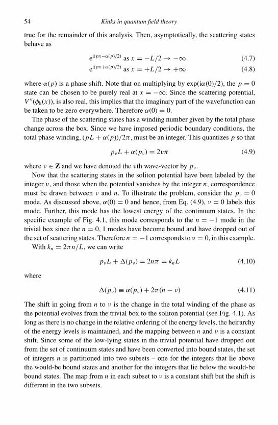
54 Kinks in quantum field theory
true for the remainder of this analysis. Then, asymptotically, the scattering statesbehave as
ei(px−α(p)/2) as x = −L/2 → −∞ (4.7)
ei(px+α(p)/2) as x = +L/2 → +∞ (4.8)
where α(p) is a phase shift. Note that on multiplying by exp(iα(0)/2), the p = 0state can be chosen to be purely real at x = −∞. Since the scattering potential,V ′′(φk(x)), is also real, this implies that the imaginary part of the wavefunction canbe taken to be zero everywhere. Therefore α(0) = 0.
The phase of the scattering states has a winding number given by the total phasechange across the box. Since we have imposed periodic boundary conditions, thetotal phase winding, (pL + α(p))/2π , must be an integer. This quantizes p so that
pν L + α(pν) = 2νπ (4.9)
where ν ∈ Z and we have denoted the νth wave-vector by pν .Now that the scattering states in the soliton potential have been labeled by the
integer ν, and those when the potential vanishes by the integer n, correspondencemust be drawn between ν and n. To illustrate the problem, consider the pν = 0mode. As discussed above, α(0) = 0 and hence, from Eq. (4.9), ν = 0 labels thismode. Further, this mode has the lowest energy of the continuum states. In thespecific example of Fig. 4.1, this mode corresponds to the n = −1 mode in thetrivial box since the n = 0, 1 modes have become bound and have dropped out ofthe set of scattering states. Therefore n = −1 corresponds to ν = 0, in this example.
With kn = 2πn/L , we can write
pν L + (pν) = 2nπ = kn L (4.10)
where
(pν) ≡ α(pν) + 2π (n − ν) (4.11)
The shift in going from n to ν is the change in the total winding of the phase asthe potential evolves from the trivial box to the soliton potential (see Fig. 4.1). Aslong as there is no change in the relative ordering of the energy levels, the heirarchyof the energy levels is maintained, and the mapping between n and ν is a constantshift. Since some of the low-lying states in the trivial potential have dropped outfrom the set of continuum states and have been converted into bound states, the setof integers n is partitioned into two subsets – one for the integers that lie abovethe would-be bound states and another for the integers that lie below the would-bebound states. The map from n in each subset to ν is a constant shift but the shift isdifferent in the two subsets.
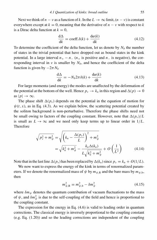
4.1 Quantization of kinks: broad outline 55
Next we think of n − ν as a function of k. In the L → ∞ limit, (n − ν) is constanteverywhere except at k = 0, meaning that the derivative of n − ν with respect to kis a Dirac delta function at k = 0,
d
dk= coeff.δ(k) + dα(k)
dk(4.12)
To determine the coefficient of the delta function, let us denote by Nb the numberof states in the trivial potential that have dropped out as bound states in the kinkpotential. In a large interval n+ − n− (n+ is positive and n− is negative), the cor-responding interval in ν is smaller by Nb, and hence the coefficient of the deltafunction is given by −2π Nb
d
dk= −Nb2πδ(k) + dα(k)
dk(4.13)
For large momenta (and energy) the modes are unaffected by the deformation ofthe potential at the bottom of the well. Hence pν → kn in this region and (p) → 0as |p| → ∞.
The phase shift (pν) depends on the potential in the equation of motion forψ(t, x), as in Eq. (4.3). As we explain below, the scattering potential created bythe soliton background is non-perturbative. Therefore the phase shifts need notbe small owing to factors of the coupling constant. However, note that (pν)/Lis small as L → ∞ and we need only keep terms up to linear order in 1/L .Therefore
√p2
ν + m2ψ =
√(kn − (pν)
L
)2
+ m2ψ
=√
k2n + m2
ψ − kn(kn)
L√
k2n + m2
ψ
+ O
(1
L2
)(4.14)
Note that in the last line (pν) has been replaced by (kn) since pν = kn + O(1/L).We now want to express the energy of the kink in terms of renormalized param-
eters. If we denote the renormalized mass of ψ by mψ,R and the bare mass by mψ,b,then
m2ψ,R = m2
ψ,b − δm2ψ (4.15)
where δmψ denotes the quantum contribution of vacuum fluctuations to the massof ψ , and δm2
ψ is due to the self-coupling of the field and hence is proportional tothe coupling constant.
The expression for the energy in Eq. (4.6) is valid to leading order in quantumcorrections. The classical energy is inversely proportional to the coupling constant(e.g. Eq. (1.20)) and so the leading corrections are independent of the coupling
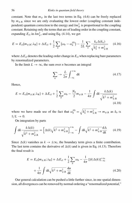
56 Kinks in quantum field theory
constant. Note that mψ in the last two terms in Eq. (4.6) can be freely replacedby mψ,R since we are only evaluating the lowest order (coupling constant inde-pendent) quantum correction to the energy and δm2
ψ is proportional to the couplingconstant. Retaining only the terms that are of leading order in the coupling constant,expanding Ecl in δm2
ψ , and using Eq. (4.14), we get
E = Ecl[mψ,R; λR] + Ecl + 1
2
∑b
(ωb − ω
(0)b
)− 1
2L
∑n
kn(kn)√k2
n + m2ψ,R
(4.16)
where Ecl denotes the leading order change in Ecl when replacing bare parametersby renormalized parameters.
In the limit L → ∞, the sum over n becomes an integral
∑n
→ L
2π
∫ +∞
−∞dk (4.17)
Hence,
E = Ecl[mψ,R; λR] + Ecl + 1
2
∑b
ωb − Nb
2mψ,R − 1
4π
∫dk
k(k)√k2 + m2
ψ,R
(4.18)
where we have made use of the fact that ω(0)b =
√k2
b + m2ψ,R → mψ,R as kb ∝
1/L → 0.On integration by parts∫
dkk(k)√
k2 + m2ψ,R
=[(k)
√k2 + m2
ψ,R
]+∞
−∞−∫
dk√
k2 + m2ψ,R
d
dk(4.19)
Since (k) vanishes as k → ±∞, the boundary term gives a finite contribution.The last term contains the derivative of (k) and is given in Eq. (4.13). Thereforethe final result is
E = Ecl[mψ,R; λR] + Ecl + 1
2
∑b
ωb − 1
4π[|k|(k)]+∞
−∞
+ 1
4π
∫dk√
k2 + m2ψ,R
dα
dk(4.20)
Our general calculation can be pushed a little further since, in one spatial dimen-sion, all divergences can be removed by normal ordering a “renormalized potential,”
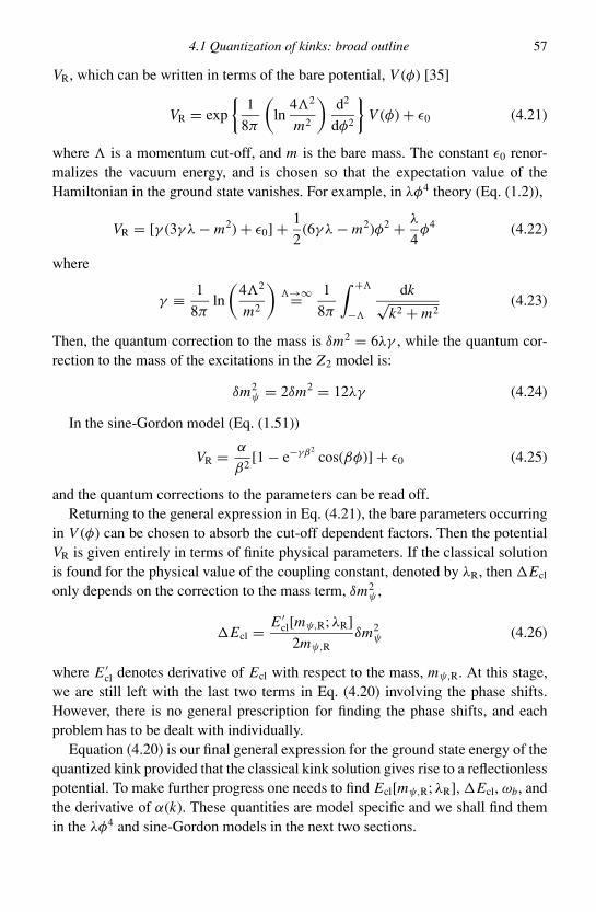
4.1 Quantization of kinks: broad outline 57
VR, which can be written in terms of the bare potential, V (φ) [35]
VR = exp
1
8π
(ln
42
m2
)d2
dφ2
V (φ) + ε0 (4.21)
where is a momentum cut-off, and m is the bare mass. The constant ε0 renor-malizes the vacuum energy, and is chosen so that the expectation value of theHamiltonian in the ground state vanishes. For example, in λφ4 theory (Eq. (1.2)),
VR = [γ (3γ λ − m2) + ε0] + 1
2(6γ λ − m2)φ2 + λ
4φ4 (4.22)
where
γ ≡ 1
8πln
(42
m2
)→∞= 1
8π
∫ +
−
dk√k2 + m2
(4.23)
Then, the quantum correction to the mass is δm2 = 6λγ , while the quantum cor-rection to the mass of the excitations in the Z2 model is:
δm2ψ = 2δm2 = 12λγ (4.24)
In the sine-Gordon model (Eq. (1.51))
VR = α
β2[1 − e−γβ2
cos(βφ)] + ε0 (4.25)
and the quantum corrections to the parameters can be read off.Returning to the general expression in Eq. (4.21), the bare parameters occurring
in V (φ) can be chosen to absorb the cut-off dependent factors. Then the potentialVR is given entirely in terms of finite physical parameters. If the classical solutionis found for the physical value of the coupling constant, denoted by λR, then Ecl
only depends on the correction to the mass term, δm2ψ ,
Ecl = E ′cl[mψ,R; λR]
2mψ,Rδm2
ψ (4.26)
where E ′cl denotes derivative of Ecl with respect to the mass, mψ,R. At this stage,
we are still left with the last two terms in Eq. (4.20) involving the phase shifts.However, there is no general prescription for finding the phase shifts, and eachproblem has to be dealt with individually.
Equation (4.20) is our final general expression for the ground state energy of thequantized kink provided that the classical kink solution gives rise to a reflectionlesspotential. To make further progress one needs to find Ecl[mψ,R; λR], Ecl, ωb, andthe derivative of α(k). These quantities are model specific and we shall find themin the λφ4 and sine-Gordon models in the next two sections.
58 Kinks in quantum field theory
Before going on to some examples, it is helpful to track the coupling constantdependence of the various terms in Eq. (4.16). We write the potential as
V (φ) = −m2
2φ2 + εS(φ) (4.27)
where m is the mass parameter, ε is the small coupling constant, and S is someunspecified function of φ, perhaps containing other parameters. The classical energyterm in Eq. (4.16) is inversely proportional to the coupling constant. So the leadingorder correction is independent of the coupling constant. In the second term, δm2
ψ
is proportional to the coupling constant but E ′cl is inversely proportional to the
coupling constant. Hence the product is independent of the coupling constant. Nextwe come to the coupling constant dependence of the energy eigenvalues and thephase shifts. The spectrum of excitations is found by solving for eigenmodes inthe kink background. The kink background provides a potential with which theexcitations interact. The important point here is that this potential is non-trivialeven to zeroth order in the coupling constant. The vacuum expectation value of φ,denoted by φ0, is found by minimizing V . Therefore
S′(φ0)
φ0= m2
ε(4.28)
Then
V ′′(φ0) = −m2 + εS′′(φ0) (4.29)
and approximating S′′(φ0) as S′(φ0)/φ0,
V ′′(φ0) ∼ −m2 + εS′(φ0)
φ0∼ m2 (4.30)
Hence the scattering potential in Eq. (4.3) for the mode functions is independentof the coupling constant, and the phase shifts, α(k), are non-trivial even to zerothorder in the coupling constant.
As we see in the specific examples given below, both δm2ψ and the last sum in
Eq. (4.16) are divergent. However, the divergences cancel, leading to a finite resultfor the energy.
4.2 Example: Z2 kink
We now find the energy of the quantized Z2 kink by evaluating explicitly the termsin Eq. (4.16).
The classical energy piece is already known from Eq. (1.20)
Ecl[mψ,R; λR] = 2√
2
3
m3
λR= m3
ψ,R
3λR(4.31)
4.2 Example: Z2 kink 59
Then Ecl is given by Eq. (4.26) and E ′cl is found by differentiating Eq. (4.31)
E ′cl[mψ,R; λR] = m2
ψ,R
λR(4.32)
The mass correction δm2ψ arises owing to the interaction term λφ4/4 in this
model. The calculation of δm2ψ is quite involved since it requires renormalization
in a model with spontaneous symmetry breaking, which means that we shouldfind the mass correction from the action in Eq. (1.5). Then there are both cubicand quartic interactions. This calculation can be found in quantum field theorytextbooks, for example [119]. The end result is
δm2ψ = 3λR
2π
∫dk√
k2 + m2ψ,R
(4.33)
The integral in Eq. (4.33) is divergent. However it is only one term in the expressionfor the quantum kink energy in Eq. (4.18). In particular, the last term with thephase shifts is also divergent, but the quantum kink energy is finite since the twodivergences cancel. Note that we can replace mψ by mψ,R in the final integral sincewe are only evaluating the leading order correction.
Next consider the terms in Eq. (4.16) that involve the spectrum of fluctuationsabout the classical kink. To find the spectrum, substitute Eq. (4.1) in the fieldequation, Eq. (1.4), and expand to lowest non-trivial order in ψ . This was alreadydone in Section 3.2 and we now summarize the results
ω0 = 0, χ0 = sech2z
ω1 =√
3
2mψ, χ1 = sinhz sech2z
mψ < ω < ∞, χk = eikx [3 tanh2z − 1 − w2k2 − i 3wk tanhz]
where z = x/w = mψ x/2, and the dispersion relation is
ω2k = k2 + m2
ψ (4.34)
Note that the eigenvalues ωk are independent of the coupling constant because λ
does not occur in Eq. (3.10) if mψ = √2λη is held fixed. However, this statement
is only true to leading order in λ because the mass parameter, the kink width, andindeed the form of the kink solution get modified owing to quantum corrections,and induce λ dependence in the spectrum. Since we are only working to leadingorder in quantum corrections, the mass parameter mψ entering Eq. (3.10) and thedefinition of the kink width, w, are the same as mψ,R.

60 Kinks in quantum field theory
The next step is to impose periodic boundary conditions with period L → ∞ onthe scattering state. For this we find the asymptotic behavior of χk
χk → eikz(2 − w2k2 ∓ i 3wk) ∝ expi(kz ± α(k)/2), z → ±∞ (4.35)
from which the phase shifts follow
α(k) = 2 tan−1
[3wk
w2k2 − 2
](4.36)
Hence
dα
dk= −6w
w2k2 + 2
(w2k2 + 1)(w2k2 + 4)(4.37)
and
(k) → 6
wk, |k| → ∞ (4.38)
Now we combine all the terms in Eq. (4.20)
E = m3ψ,R
3λR+
√3
4mψ,R − 3
2πmψ,R − 3m3
ψ,R
16π
∫ +∞
−∞
dk√k2 + m2
ψ,R
1
k2 + m2ψ,R/4
(4.39)
The last integral is done easily yielding the final result for the kink mass withleading order quantum correction
E = m3ψ,R
3λR−(
3
π− 1
2√
3
)mψ,R
2
= m3ψ,R
3λR− 0.33mψ,R (4.40)
Note the minus sign in front of the quantum correction to the energy. In Section 4.5we show that this is a general feature.
4.3 Example: sine-Gordon kink
To quantize the sine-Gordon kink of Section 1.9, we follow the same procedure asfor the Z2 kink. The mode functions now satisfy
−d2ψ
dX2+ (2 tanh2 X − 1)ψ = ω2
m2ψ
ψ (4.41)

4.3 Example: sine-Gordon kink 61
where X ≡ mψ x . The kink solution, from Eq. (1.52), is
φk = 4
βtan−1
(e√
αx) ≡ 4mψ√
λtan−1
(emψ x
)(4.42)
where λ ≡ αβ2. The classical energy (Eq. (1.55)) is
EsG,cl = 8
√α
β2≡ 8
m3ψ
λ(4.43)
The spectrum has only one bound state, the translational zero mode given by
ω1 = 0, ψ0 = dφk
dx= 2m2
ψ√λ
sech(mψ x) (4.44)
The scattering state with wave-vector k can be written quite generally in terms ofhypergeometric functions (see [113], Vol. II, Section 12.3, or Appendix C)
ψκ = N (cosh X )iκ X F
(−iκ − 1, −iκ + 1
2+ 3
2|1 − iκ| e−X
eX + e−X
)(4.45)
where N is a normalization factor and κ = k/mψ corresponds to the wave-vector.The phase shifts are found by taking the asymptotic forms of Eq. (4.45)
ψκ → Neiκ X , X → ∞→ Nei(π+2θ )eiκ X , X → −∞ (4.46)
where tan θ = κ . Hence the phase shift is
αk = π − 2 tan−1
(k
mψ
)(4.47)
Therefore
dαk
dk= −2mψ
k2 + m2ψ
(4.48)
At large |k|, (k) (as needed in Eq. (4.20)) is given by
(k) = 2mψ
k, |k| → ∞ (4.49)
To find Ecl occurring in Eq. (4.20), we can use the renormalized potential inEq. (4.25). The parameter β, which occurs in the argument of the cosine function,is taken to be the physical (renormalized) value, while
(√
α)b = (√
α)R
(1 + β2
2γ
)(4.50)

62 Kinks in quantum field theory
to leading order in β2. The subscripts refer to bare and renormalized quantities andγ is defined in Eq. (4.23). Therefore
Ecl = mψ,R
2π
∫ +
−
dk√k2 + m2
ψ
(4.51)
Finally, with∑
ωb = 0, we can put together all the various terms in Eq. (4.20)to get
E = 8m3ψ,R
λR+ mψ,R
2π
∫ +
−
dk√k2 + m2
ψ
+ 0 − mψ,R
π− mψ,R
2π
∫ +
−
dk√k2 + m2
ψ
= 8m3ψ,R
λR− mψ,R
π
= 8m3ψ,R
λR− 0.32mψ,R (4.52)
Once again the quantum correction is negative and, coincidentally, quite close tothe Z2 value (see Eq. (4.40)).
4.4 Quantized excitations of the kink
So far we have only calculated the quantum correction to the mass of the kink inits ground state. Now consider the excited states of the kink.
As in the second quantization of a free quantum field theory, particle creationand annhilation operators are introduced for each of the excitation modes of thekink. As we shall see, this is straightforward except for the zero mode. The endresult is a procedure for doing quantum field theory with both particles and kinksincluded in the spectrum of states. Here we only give some introductory remarks.For a more extended discussion see [67, 126].
Let us denote the bound state mode functions by Fb(t, x) and the scatteringmode functions by fk(t, x). The t dependence is of the form exp(−iωi t) where ωi
is the frequency of the bound or scattering mode. Then the second quantized fieldoperator is
φ = φk(x) +∑
b
[cb Fb(t, x) + c†b F∗
b (t, x)]+
∑k
[ak fk(t, x) + a†
k f ∗k (t, x)
](4.53)
where φk is the classical kink solution, c†b, cb are creation/annihilation operatorsfor the bound states, and similarly a†
k , ak are creation/annihilation operators for thescattering states. Now, for the zero mode, ω = 0 and F0(t, x) = F∗
0 (t, x). Therefore
4.5 Sign of the leading order correction 63
the zero mode contribution to the sum is
[c0 + c†0]F0(x) (4.54)
Since c0 and c†0 are only present in the combination c0 + c†0 let us define b0 = c0 + c†0which is then the annihilation operator for the zero mode. However, note thatb†
0 = b0 and so [b0, b†0] = [b0, b0] = 0: the zero mode is classical as the operator
b0 commutes with all other operators. This is to be contrasted with [ak, a†p] =
2πδ(k − p).Just as the translation mode is a bosonic zero mode, there can also be fermionic
zero modes that we discuss in Chapter 5. In that case, the creation and annihilationoperators satisfy anticommutation relations leading to b0, b†
0 = 0. This relationhas the remarkable consequence of leading to fractional quantum numbers as wediscuss in Chapter 5.
4.5 Sign of the leading order correction
A striking feature of the leading order quantum corrections to the energies of theZ2 and sine-Gordon kink is that they are negative. In other words, quantum effectsreduce the mass of the kink. A variational argument [104] (Coleman, S., 1992,private communication) shows that this observation holds true quite generally inone dimension.1
Let the Hamiltonian of the 1 + 1 dimensional system be
H ≡∫
dxH =∫
dx [H0 + V (φ)] (4.55)
where φ is a scalar field,
H0 ≡ 1
2π2 + 1
2(∂xφ)2 (4.56)
and π is the canonical field momenta. Written in this way, the parameters enteringthe Hamiltonian are bare parameters and subject to renormalization. In one spatialdimension, however, it can be shown that [35]
H = Nm [H0 + VR] (4.57)
where Nm denotes normal ordering with respect to free particles of mass m, andthe renormalized potential is (Eq. (4.21))
VR = exp
1
8π
(ln
42
m2
)d2
dφ2
V (φ) + ε (4.58)
1 The conclusion may not hold if the model also contains fermionic fields.
64 Kinks in quantum field theory
where is an ultraviolet momentum cut-off and ε is a constant to be chosen suchthat 〈0|H |0〉 = 0 where |0〉 is the true ground state of the model.
The energy of the kink, including the contribution of quantum fluctuations in theground state, is
E = k〈0|H [φk + ψ]|0〉k (4.59)
where |0〉k denotes the vacuum for the quantum fluctuations, ψ , around the classicalone kink state φk.
Straightforward manipulation now gives the quantum correction to the kink mass
E − Ecl,R = k〈0|H [φk + ψ] − H [φk]|0〉k
=∫
dx k〈0|Nm(H0[φk + ψ] − H0[φk] + VR[φk + ψ] − VR[φk])|0〉k
where Ecl,R is the energy of the classical solution obtained with the renormalizedpotential, VR. Next we use the variational principle, which states that the groundstate energy of a system is minimized in its true ground state, and the expectationof the Hamiltonian in any other trial state gives an upper bound to the ground stateenergy. If we denote the perturbative vacuum state – the state with zero particles ofmass m – by |0, m〉, then
E ≤ Ecl,R +∫
dx 〈0, m|Nm(H0[φk + ψ] − H0[φk] + VR[φk + ψ] − VR[φk])|0, m〉= Ecl,R
The last line follows since there are no ψ independent terms in the expectationvalue under the integral,2 and the annihilation operators of ψ occur to the rightowing to normal ordering and annihilate the trial vacuum state.
Note that Ecl,R is the energy of the classical solution found by minimizing HR[φ],i.e. the Hamiltonian in Eq. (4.55) but with the potential given in Eq. (4.58). Since thetrue ground state of the system is not known, the constant ε is not known either. Thepotential VR can be minimized, but there is no guarantee that the minimal value ofVR will be zero. Therefore Ecl,R might get an infinite contribution from integratingmin(VR) over all of space. Then the variational bound E ≤ Ecl,R is not very useful.However, we do know the value of ε to lowest order in the coupling constant andthis is precisely so that 〈0, m|H |0, m〉 = 0. This coincides with choosing ε so as tomake min(VR) = 0. Hence the bound
E ≤ Ecl,R = Ecl (4.60)
2 To see this, note that the expectation value vanishes if ψ = 0.
4.6 Boson-fermion connection 65
where Ecl denotes the classical energy without any quantum corrections, is mean-ingful to leading order in perturbation theory and it provides us with the completelygeneral result that the lowest order correction to the soliton energy is negative.
4.6 Boson-fermion connection
A bosonic field, φ, in quantum field theory satisfies the equal time commutationrelation
[φ(x, t), φ(y, t)] = δ(x − y) (4.61)
Alternatively, a fermionic field, ψ , satisfies the anticommutation relations
ψa(x, t), ψ†b(y, t) = δ(x − y)δab (4.62)
where a, b = 1, 2 label the two components of the spinor in one spatial dimension.It is remarkable that one can construct explicitly a fermionic field ψ satisfyingEq. (4.62) in terms of a bosonic field φ that satisfies Eq. (4.61) [108].
The connection between ψa and φ is
ψ1(x) = C : eP+(x) :, ψ2(x) = −iC : eP−(x) : (4.63)
where the c-number C is defined in terms of a mass parameter µ and another cut-offparameter, ε,
C =( µ
2π
)1/2eµ/8ε (4.64)
The operators P± contain a free parameter β and are defined by
P±(x) = −i2π
β
∫ x
−∞dξ φ(ξ ) ∓ iβ
2φ(x) (4.65)
The symbol :: in Eq. (4.63) denotes normal ordering with respect to the mass µ.This means that the field φ is to be treated as a free field with mass parameterµ and the quantum operator, φ, is expanded in terms of creation and annihilationoperators that create and destroy particles of this free field theory. A normal orderedoperator contains various products of creation and annihilation operators with theannihilation operators always occurring on the right. It is understood that the in-tegral in Eq. (4.65) is cut off at large ξ by a factor exp(−εξ ). Note that normalordering is a symbol and should be treated carefully – normal ordering of stringsof operators should be done prior to commuting operators that occur within thestring.
66 Kinks in quantum field theory
To check if Eq. (4.62) is satisfied for x = y, we use the identity (see Appendix D)3
: eA+B := e−[A+,B−] : eA :: eB := e−[B+,A−] : eB :: eA : (4.66)
where A and B are any two operators that can be written as a linear sum of termsinvolving only creation or annihilation operators
A = A+ + A−, B = B+ + B− (4.67)
The commutators [A+, B−] and [B+, A−] are assumed to be c-numbers. Insertionof Eq. (4.66) in Eq. (4.62) gives the commutation relation in Eq. (4.61) for x = y.
It is harder to check that the commutation relations in Eq. (4.61) hold whenx = y. Since products of quantum operators at the same point are singular, thecommutator must be evaluated at two different points in space, x and y, followedby the coincidence limit y → x . We now outline the scheme employed in [108].
We want to check the anticommutation relation
ψa(x), ψ†b(y) = Zδ(x − y) (4.68)
where the constant Z , possibly infinite, has been introduced in recognition of thefact that the fields get renormalized. Rather than check Eq. (4.68), we can checkthe equivalent commutation relation
[ jµ(x), ψ(y)] = −(
g0µ + β2
4πεµ0γ 5
)ψ(x)δ(x − y) (4.69)
where the current jµ has been regularized using point-splitting and is defined by
jµ(x) = limy→x
[δµ0 + β2
4πδ
µ
1
][µ(x − y)]σ ψ(x)γ µψ(y) + Fµ(x − y)
(4.70)
where σ is a regularizing parameter and Fµ(x − y) an unspecified c-valued func-tion. The γ -matrices are defined by the algebra
γ µ, γ ν = 2gµν, γ 5 = iγ 0γ 1 (4.71)
where gµν = diag(1, −1) is the two-dimensional Minkowski metric. An explicitrepresentation of the γ -matrices is given in Eq. (5.15). In Eq. (4.69), εµν is thetotally antisymmetric tensor.
First the current jµ is evaluated with ψa as given in Eq. (4.63). The evaluationrequires
[φ+(x, t2), φ−(y, t1)] = +[(x − y)2 − (dt + iε)2] (4.72)
3 In the literature it is sometimes incorrectly stated that the identity eA+B = e[B,A]/2eAeB (no normal ordering)is being used.
4.7 Equivalence of sine-Gordon and massive Thirring models 67
where dt = t2 − t1 and + is the propagator. For small x − y
+ = − 1
4πln[µ2(x − y)2 − (dt + iε)2] + O((x − y)2) (4.73)
By differentiating Eq. (4.72) we can also obtain the commutators of time derivativesof φ+ and φ−. These appear in the evaluation of jµ since ψ is defined in terms ofφ in Eq. (4.63).
The result for jµ is singular in the limit y → x except for a single choice of theregularizing parameter, σ , occurring in the definition of jµ. This single choice is
σ = β2
8π
(1 − 4π
β2
)2
(4.74)
With this value of σ , the commutator in Eq. (4.69) can be verified. Thus theψ operator indeed satisfies the anticommutation relations of a fermionic field.Furthermore, the current can be explicitly calculated, leading to
jµ = − β
2πεµν∂νφ (4.75)
To summarize, given a quantum scalar field in 1 + 1 dimensions, it is possi-ble to construct a fermionic field from it via the relation (4.63). Starting with afermionic field, a bosonic field may be constructed from it via Eq. (4.75). Note thatthe transformations from bosons to fermions and vice versa hold at the quantumoperator level and not just at the level of expectation values. Further, they holdfor any choice of interactions in the bosonic or the fermionic model. However, inthe case when the bosonic model is the sine-Gordon model, the fermionic modelobtained by transforming to the fermionic variables is another well-known model,namely the massive Thirring model as we now describe.
4.7 Equivalence of sine-Gordon and massive Thirring models
The sine-Gordon model is given by the Lagrangian (Eq. (1.51))
LsG = 1
2(∂µφ)2 − α
β2(1 − cos(βφ)) (4.76)
while the massive Thirring model is
LmT = iψ ∂ψ − mψψ − g
2ψγ µψ ψγµψ (4.77)
where ψ is a two-component fermionic field.In [34] (also see [35]) it is shown that the sine-Gordon model does not have a
well-defined ground state for β2 > 8π . To clarify what this means, consider the

68 Kinks in quantum field theory
simple example of a free field theory
L free = 1
2(∂µφ)2 − δ
2φ2 (4.78)
This model has a well-defined ground state only in the range δ ≥ 0. The model doesnot have a well-defined ground state for δ < 0. Similarly the sine-Gordon modelonly has a ground state for a definite range of parameters, though the reasons aremuch more subtle.4 The sine-Gordon only has a well-defined ground state if theparameter β2 is restricted to lie in the interval (0, 8π ).
In the range, 0 ≤ β2 ≤ 8π , there is a one-to-one mapping between vacuumexpectation values of a string of operators in the sine-Gordon model to those inthe massive Thirring model. This means that any vacuum expectation value in thesine-Gordon model has a “corresponding” vacuum expectation value in the massiveThirring model. This strongly suggests that the two models are equivalent, even atthe operator level [35].
As we have seen in the last section, there is indeed a two-component fermionicfield, ψ , that can be constructed from a bosonic field φ (Eq. (4.63)). In [108] it wasshown that ψ also obeys the equations of motion of the massive Thirring modelif the bosonic field φ obeys the equations for the sine-Gordon equation with thecoupling constant g written in terms of the coupling constant β as
g
π= 1 − 4π
β2(4.79)
Note that when the sine-Gordon model is weakly coupled (small β), the massiveThirring model is strongly coupled and vice versa. Hence the sine-Gordon modeland the massive Thirring model are completely equivalent as quantum field theoriesbut one is a better description at small β (large g) and the other at large β (small g).
What has the equivalence of the sine-Gordon and massive Thirring models gotto do with kinks? Consider the commutation relations between φ and ψ . UsingEq. (4.63) and the identity (see Appendix D) [A, : eB : ] =: [A, eB] : with A =φ(y) and : eB := ψ we find
[φ(y), ψ(x)] = 2π
βψ(x), (y < x) (4.80)
[φ(y), ψ(x)] = 0, (y > x) (4.81)
Now consider the action of ψ(x) on an eigenstate, |s〉 of the field operator φ. Letus choose this eigenstate to be such that
φ|s〉 = 0 (4.82)
4 For example, in contrast to the model in Eq. (4.78), the classical sine-Gordon model has well-defined globalminima for all values of the coupling constant β.
4.7 Equivalence of sine-Gordon and massive Thirring models 69
If we write |s ′〉 = ψ(x)|s〉, the relation in Eq. (4.80) gives
φ(y)|s ′〉 = 2π
β|s ′〉, (y < x) (4.83)
and Eq. (4.81) gives
φ(y)|s ′〉 = 0, (y > x) (4.84)
Therefore the state obtained after action by ψ(x) is one where the value of φ is 2π/β
for y < x and 0 for y > x . In other words, the field ψ(x) creates a step-change of φ.The step-function profile is viewed as a “bare kink” which gets dressed by quantumeffects that produce a smooth kink profile with some finite width. So the field ψ(x)is the creation operator for a (bare) soliton at location x . In the Thirring model, thefield ψ(x) is interpreted as the creation operator for a fermion located at x . Hencethe sine-Gordon kink is identified with the fermion in the massive Thirring model.
The topological charge on a sine-Gordon kink is
Qk =∫
dx j0B =
∫dx j0
F (4.85)
where the fermionic current is defined in terms of the bosonic current in Eq. (4.75).Therefore the fermion in the massive Thirring model carries the topological chargeof the sine-Gordon kink. In other words, the kink of the strongly coupled sine-Gordon model is better described as a weakly coupled fermion of the massiveThirring model. Here we see the duality between particles and solitons.
Can we also interpret the bosonic particles of the sine-Gordon model in terms of“solitons” of the massive Thirring model? The massive Thirring model only containsfermions, and classical solutions of the Dirac equation do not have the interpretationof solitons. This is because the fermionic fields anticommute and fermions obey thePauli exclusion principle. Instead a classical solution of the Dirac equation is a statethat one (and only one) fermion can occupy. However, there can be bound statesof two or more fermions since the force between a fermion and an antifermion isattractive for g > 0. A bound state of two fermions can be shown to correspond toa particle of the sine-Gordon field φ. If the fermions in the weakly coupled massiveThirring model have mass m, then the bound state energy is approximately 2msince it involves two fermions. However, the binding energy decreases (becomesmore negative) with increasing interaction strength, g, and eventually the boundstate becomes lighter than a single fermion. At this stage, a suitable description ofthe system is in terms of the bound state being the fundamental degree of freedomas in the sine-Gordon model.
The bound state of two massive Thirring fermions is also a bound state oftwo sine-Gordon kinks i.e. a breather. Hence it should be possible to interpret

70 Kinks in quantum field theory
the breather as a particle in the sine-Gordon model. This is seen to be true when thebreather is quantized [38–41, 35]. Then, to lowest order, the energy levels ofthe quantized breather are equal to the mass of one, two, three, etc. particles ofthe sine-Gordon particle.
4.8 Z2 kinks on the lattice
Lattice field theory provides another tool to probe the quantum nature of solitonsand, in particular, the variation of mass with coupling constant.
The starting point is the action for the Z2 model defined in Eq. (1.2). The actionis to be inserted in the Feynman path integral, which can then be used to findexpectation values for any quantum operator. In the Feynman path integral, it isnecessary to integrate over field configurations, and this is done numerically on adiscretized Euclidean space-time. The reader is referred to the lattice literature fordetails [37, 112, 141]. Here we shall give the results relevant to the Z2 kink.
The mass of a Z2 kink is defined as the expectation value of a suitable operatordefined on the lattice in the limit that the lattice spacing, a, goes to zero. Oneimportant issue is that there are several different candidate operators on the latticethat all go to the correct limit as a → 0 and, in practice, it is not possible to take thelimit all the way to a = 0. At best, the numerical analysis gives the expectation ofthe operator on the lattice for several different values of a and then some schememust be found for extrapolating the results to a → 0. In [32], the authors evaluatethe mass of the Z2 kink using two different lattice operators. The results are shownin Fig. 4.2. We note that the kink mass decreases monotonically as the couplingconstant increases and remains bounded by the classical mass. At a certain coupling,the kink mass goes to zero, and the kink, not the φ quanta, is the lightest degree offreedom in the model.
The mass of the sine-Gordon kink has been calculated analytically for a rangeof parameters in [156] (also see [35]).
4.9 Comments
Several researchers have taken alternate paths to studying quantized kinks. Insupersymmetric theories there is greater control over quantum corrections and themass can, in some cases, be evaluated exactly [51]. Alternate methods to quantizesupersymmetric kinks have also been developed in [66]. Variational methods tostudy the λφ4 theory have been developed in [49]. The scattering of kinks in classi-cal and quantum theory has been studied in [153]. Kink masses and scattering havealso been calculated in [132] using the Hartree approximation.

4.10 Open questions 71
Classical prediction
msol
ʃ Ω(β)
b0
Theor. [O(h)]
0.05 0.10 0.15 0.20 0.25 0.30 0.35
5
4
3
2
1
0
Figure 4.2 The figure shows how the mass of the Z2 kink depends on the inversecoupling constant, β0 = 1/λ0, where λ0 ≡ 6λa2 is the coupling constant in thediscrete theory on a 48 × 48 lattice and a is the lattice spacing. (The factor of 6is due to our choice of 1/4 in the λ term in Eq. (1.2) as opposed to 1/4! in [32].)The lattice mass parameter, r0 ≡ −m2a2, is held fixed at r0 = −2.2. From theplot we see that the classical value of the kink mass is larger than the quantumvalue. The one-loop corrected mass (see Section 4.2) and the mass found by usingtwo different choices of the lattice mass operator are also shown. The kink massvanishes at β0 = 0.0804. [Figure reprinted from [32].]
The construction of fermion operators from boson operators and vice versa hasbeen discussed and used extensively in condensed matter applications under thename of bosonization. A review, in addition to an historical introduction, may befound in [44]. Finally, the technique of bosonization has also been applied to thermalsystems in [69].
4.10 Open questions
1. The quantum corrections to the Z2 and sine-Gordon kinks were calculated explicitly usingthe phase shifts. However, the phase shift approach only works if the potential U (x) isreflectionless. What are the conditions necessary for a potential to be reflectionless? Arereflectionless potentials always in factorizable form (see Section 3.3)? (The example ofa step-function potential shows that the converse is not true.)
72 Kinks in quantum field theory
2. We have shown that the leading order quantum correction to the kink mass is alwaysnegative. Can this statement be generalized to all orders? Can one show that the massof a kink goes to zero in the strong coupling limit? Or perhaps that it is monotonicallydecreasing as a function of increasing coupling constant?
3. If the Z2 kink at strong coupling is to be viewed as a particle, then the particle must obeyunusual statistics because two kinks cannot be next to each other. Discuss this statisticsand its implications for the dual model.
4. From the SU (5) × Z2 example we learned that a classical kink may be embedded inmany different ways in “large” models. On quantization, do the different embeddingscorrespond to distinct degrees of freedom?
5. Does the addition of fermionic particles change the conclusion that quantum correctionsalways reduce the energy of a kink?
6. For the sine-Gordon model we have explicitly seen that there is a relation between kinksand particles. It seems reasonable that the connection holds in other models too. In 3 + 1dimensions, we could expect the connection to exist between magnetic monopoles andobserved particles (e.g. [162, 103]). Construct a model that has families of solitons,similar to the electron, muon, and tau families observed in Nature (see [122]).
7. In Section 3.1 we have discussed the existence of quasi-breather solutions called“oscillons” in the Z2 model. Can quantum oscillons have an interpretation that is similarto quantized breathers as discussed at the end of Section 4.7?
5
Condensates and zero modes on kinks
In this chapter we study the effect of a kink on other bosonic or fermionic fields thatmay be present in the system. Under certain circumstances, it might be energeticallyfavorable for a bosonic field, denoted by χ , to become non-trivial within the kink.Then we say that there is a “bosonic condensate” which is trapped on the kink.On a domain wall, the condensate has dynamics that are restricted to lie on theworld-sheet of the wall.
The situation is similar for a fermionic field though there are subtleties. For afermionic field, denoted by ψ , the Dirac equation is solved in the presence of akink background made up of bosonic fields. This determines the various quantummodes that the fermionic excitations can occupy. In several cases, there can be“zero modes” of fermions in the background of a kink and this leads to severalnew considerations. (Fermionic zero modes were first discovered in [27, 84] in thecontext of strings.) In addition to the zero mode, there may be fermionic boundstates. The high energy states that are not bound to the wall are called “scattering(or continuum) states.”
A difference between bosonic and fermionic condensates is that bosonic solu-tions can be treated classically but fermionic solutions can only be interpreted inquantum theory. For example, while there may be a bosonic solution with χ = 0,the solution ψ = 0 of the Dirac equation has no meaning because this solutionis not normalizable. Solutions of the Dirac equation are only meant to supply uswith the modes that fermionic particles or antiparticles can occupy, and as suchare required to be normalizable. It is a separate issue to decide if the modes areoccupied or not. A mode contributes to the energy of the soliton only if it is occu-pied. This is quite different from the bosonic case in which there can be a classicalcondensate, on top of which there are modes that may or may not be occupiedby bosonic particles. Fermions can form a classical condensate only after theyhave paired up to form bosons (“Cooper pairs”), and this leads to superfluidity orsuperconductivity.
73
74 Condensates and zero modes on kinks
Fermionic zero modes can lend solitons some novel properties such as fractionalquantum numbers (see Section 5.3).
5.1 Bosonic condensates
Consider the model
L = Lk[φ] + 1
2(∂µχ )2 − U (φ, χ ) (5.1)
where Lk[φ] is the Lagrangian that leads to a kink solution in φ. For example, Lk
can be the Lagrangian for the Z2 or sine-Gordon models discussed in Chapter 1. χ
is another scalar field that interacts with φ via some general interaction potentialU (φ, χ ). Note that U (φ, χ ) does not contain any terms that are independent of χ –those are included in the potential, V (φ), that occurs in Lk. As an example, wecould have
U (φ, χ ) = −m2χ
2χ2 + λχ
4χ4 + σ
2φ2χ2 (5.2)
We are assuming that the parameters in the model are chosen so that the minimumof the full potential, V + U , is at φ = 0 but χ = 0. This requirement also excludesterms that are linear in χ (e.g. φ2χ).
In the fixed background of the kink, χ satisfies the classical equation of motion
∂2t χ − ∂2
x χ + Uχ (φk(x), χ) = 0 (5.3)
where Uχ denotes the derivative of U with respect to χ and φk is the kink solution.Far from the wall, the lowest energy solution is χ (±∞) = 0.
A solution to Eq. (5.3) is χ (x) = 0 and the energy of this solution is equal to thekink energy in the model Lk. However, the trivial solution may not be the one oflowest energy. To show that a lower energy solution exists, we need only show thatthe trivial solution, χ = 0, is unstable. Then we consider linearized perturbationsof the form χ = cos(ωt) f (x) around the trivial solution. Inserting this form intoEq. (5.3) leads to the Schrodinger equation
−∂2x f + Uχχ (φk(x)) f = ω2 f (5.4)
where Uχχ denotes the second derivative of V with respect to χ . If this equa-tion has solutions with ω2 < 0, it implies that there are solutions for χ on thekink background that grow with time as cosh(+|ω|t), denoting an instability ofthe state with χ = 0. This means that the solution with least energy must have anon-trivial χ configuration. The lowest energy χ configuration is non-zero insidethe kink and vanishing outside and is called a “bosonic condensate” (or simply“condensate”).
5.1 Bosonic condensates 75
5.1.1 Bosonic condensate: an example
A simple example in which there is a bosonic condensate on a Z2 kink can be foundin the model of Eq. (5.1), or explicitly,
L = 1
2(∂µφ)2 + 1
2(∂µχ )2 − λ
4(φ2 − η2)2 + m2
χ
2χ2 − λχ
4χ4 − σ
2φ2χ2 (5.5)
Ignoring the condensate field χ , the kink solution is
φk = η tanh( x
w
)(5.6)
and the Schrodinger equation corresponding to Eq. (5.4) is
−∂2x f + [− m2
χ + ση2 tanh2 X]
f = ω2 f (5.7)
where X = x/w.With ση2 > m2
χ , we see that the Schrodinger potential is asymptotically positive,and hence f (±∞) = 0. This is consistent with the requirement that χ not have avacuum expectation value. At the origin, Uχχ < 0, and hence the Schrodingerpotential is a well that is centered at the origin. Since a potential well in onedimension always has a bound state [139], it follows that there is at least one boundstate for χ . For a deep enough well i.e. large enough m2
χ , the bound state has negativeenergy eigenvalue (ω2 < 0), and the trivial solution χ = 0 is unstable. Hence thereis a range of parameters (m2
χ ) for which a χ condensate exists.To determine the range of m2
χ for which there is an instability, consider thecritical case when there is a zero eigenvalue solution, f0, of Eq. (5.7). Then we canwrite
−∂2x f0 + ση2
3[3 tanh2 X − 1] f0 =
[m2
χ − ση2
3
]f0 (5.8)
This is exactly the same form as Eq. (3.8), together with the potential in Eq. (3.10),provided we identify 3λ with σ , and ω2 with the term within square brackets onthe right-hand side. Since the lowest energy eigenvalue is zero for Eq. (3.8), thereis a zero eigenvalue for Eq. (5.7) if
m2χ = ση2
3(5.9)
For a larger value of m2χ , Eq. (5.7) has a negative eigenvalue, signaling an instability.
Therefore a condensate solution exists in the range
ση2
3< m2
χ < ση2 (5.10)
76 Condensates and zero modes on kinks
The exact profile for the condensate can be found by solving the full coupledequations of motion for φ and χ . This includes the non-linear terms in χ and theback-reaction of the condensate on the kink, and, in most cases, has to be donenumerically. Let us denote the solution obtained in this way by (φk(x), χ0(x)).Then
χ (t, x, y, z) = χ0(x) cos(ωt − ky y − kzz + θ0), ω =√
k2y + k2
z (5.11)
where θ0 is a constant, is also a solution. The reason is simply that(∂2
t − ∂2y − ∂2
z
)cos(ωt − ky y − kzz + θ0) = 0 (5.12)
The trigonometric form of the solution in Eq. (5.11) was chosen so as to obtaina real solution. An identical analysis in the case when χ is a complex field leads to
χ (t, x, y, z) = χ0(x)e±i(ωt−ky y−kz z+θ0) (5.13)
The solution represents waves propagating in the (ky, kz) direction in the plane ofthe domain wall.
5.2 Fermionic zero modes
Fermionic fields may be coupled to the kink via terms that respect the discretesymmetries in the bosonic sector that are responsible for the existence of the kink.In the case of the Z2 model, the coupling can be a Yukawa term and the Lagrangianmay be written as
L = Lφ + iψ ∂ψ − gφψψ (5.14)
where Lφ denotes the scalar part of the Lagrangian, ∂ ≡ γ µ∂µ, g is the couplingconstant, ψ is a four-component fermionic field, and γ µ are the Dirac matricesthat satisfy γ µ, γ ν = 2gµν with gµν = diag(1, −1, −1, −1) being the space-timemetric. The explicit representation of the Dirac matrices that we adopt is
γ 0 =(
0 11 0
), γ i =
(0 σ i
−σ i 0
)(5.15)
where i = 1, 2, 3 (also sometimes written as i = x, y, z) and the Pauli spin matricesare defined as
σ 1 =(
0 11 0
), σ 2 =
(0 −ii 0
), σ 3 =
(1 00 −1
)(5.16)
The Yukawa interaction term in the model in Eq. (5.14) respects the φ → −φ
symmetry of the Z2 model provided we also transform the fermion field by
5.2 Fermionic zero modes 77
ψ → ψ ′ = γ 5ψ where
γ 5 ≡ iγ 0γ 1γ 2γ 3 =(−1 0
0 1
)(5.17)
This can be seen by using the properties (γ 5)† = γ 5, γ 5, γ µ = 0 and (γ 5)2 = 1.1
If φk(x) denotes the kink solution, the Dirac equation in the kink background is
i∂ψ − gφk(x)ψ = 0 (5.18)
Let us first try and solve Eq. (5.18) explicitly. Recognizing that φk does notdepend on t , y, and z, we write the ansatz
ψ = f (t, y, z)ξ (x) (5.19)
where f (t, y, z) is a function while ξ (x) is a four-component spinor. With thisansatz, the Dirac equation separates
iγ a∂a f = −γ aka f (5.20)
iγ x∂xξ − gφkξ = +γ akaξ (5.21)
where γ aka is the constant matrix of separation and the index a runs over t, y, z.Requiring that the fermion be localized on the wall, we get the boundary conditions
ξ (±∞) = 0 (5.22)
These boundary conditions are valid only for bound states. If we wish to consider thescattering of fermions off a domain wall, we would choose incoming and reflectedplane waves at x = −∞.
The Dirac equations have an infinite number of solutions, corresponding to allthe fermion eigenmodes in the domain wall background. These include fermionicbound states and scattering states. There is one state, however, which is novelbecause it leads to some very interesting properties of the soliton, described in thesections below. This state is the one with zero energy eigenvalue, also called the“zero mode.”
Equation (5.20) can be solved
f = exp(ikaxa) ≡ exp(i(ωt − ky y − kzz)) (5.23)
Zero energy is obtained by setting ω = 0 = ky = kz and then f = 1. Let us firstlook at this case (ka = 0).
Multiplying Eq. (5.21) by iγ x we see that iγ xξ satisfies the same equation ofmotion as ξ . Therefore if ξ is a solution, then so is iγ xξ . Hence solutions to the
1 The Yukawa term does not respect the φ → φ + 2π/β symmetry of the sine-Gordon model and hence ourdiscussion of fermion zero modes cannot be used for that case. Nor do we consider the case of fermions withMajorana mass terms [147].
78 Condensates and zero modes on kinks
Dirac equation come in distinct pairs unless ξ is an eigenstate of iγ x , in which casethe two solutions ξ and iγ xξ are not distinct. The zero mode solution is found bychoosing ξ to be an eigenstate of iγ x
iγ xξ = cξ (5.24)
and, since (iγ x )2 = 1, we must have c = ±1. The ξ equation now becomes
∂xξ = cgφkξ (5.25)
and the solution is
ξ (x) = ξ (0) exp
[cg∫ x
0φk(x ′)dx ′
](5.26)
Assuming φk(+∞) > 0 and g > 0, the boundary conditions in Eq. (5.22) are onlysatisfied if c = −1. (The boundary condition at x = −∞ is also satisfied providedφk(−∞) < 0.) Therefore the zero mode solution is
ξ (x) = ξ (0) exp
[−g∫ x
0φk(x ′)dx ′
], (g > 0) (5.27)
If φk(+∞) < 0 and g > 0, the solution is obtained by choosing c = +1.To determine ξ (0), we solve the eigenvalue equation iγ xξ (0) = −ξ (0) and find
ξ (0) =
α
β
iβiα
(5.28)
where α, β are any complex constants. Therefore there are two basis zero modes(with coefficients α and β) and the general zero mode is a linear superpositionof these two modes. The constants, α and β, can be fixed by normalizing thewavefunction.
Next consider the case with ka = 0. Then Eq. (5.27) is still a solution to Eq. (5.21)provided kaγ
aξ (0) = 0. By explicitly substituting the γ a matrices and ξ (0), thisleads to the two equations
kyα + i(ω + kz)β = 0 (5.29)
i(ω − kz)α − kyβ = 0 (5.30)
A solution for α and β exists only if
ω = ±√
k2y + k2
z (5.31)
5.2 Fermionic zero modes 79
which is the dispersion relation for a massless particle (see Fig. 5.1). With thisrelation, the solutions fix the ratio of α and β to obtain
ψ = Nei(ωt−ky y−kz z)
2√
ωe−g
∫ x0 φk(x ′)dx ′
√ω + kz
sgn(ky)i√
ω − kz
−sgn(ky)√
ω − kz
i√
ω + kz
(5.32)
where N is a normalization constant where sgn(ky) ≡ ky/|ky|.So far we have not specified the exact form of the kink profile φk and Eq. (5.32)
holds for any model in which the Yukawa interaction term respects the symmetries.Next, as an example, we use the solution for the Z2 kink (see Eq. (1.9)). Then theintegral over φk can be done explicitly to yield
ψ = Nei(ωt−ky y−kz z)
2√
ω
[sech
( x
w
)]g√
2/λ
√ω + kz
sgn(ky)i√
ω − kz
−sgn(ky)√
ω − kz
i√
ω + kz
, (g > 0)
(5.33)where w is the width of the kink as defined in Eq. (1.21). This is our final expressionfor the zero mode on the Z2 kink.
In the asymptotic vacuum, where φ is constant, the Dirac equation derived fromEq. (5.14) yields four solutions all with the same momentum. These four states arereferred to as spin up and down states for the particle and hole (or antiparticle). Onthe domain wall, however, there are only two zero mode solutions for fixed valueof the momentum (ky, kz). One of these has positive energy (ω) and the other hasnegative energy. Therefore the two states may be called particle and hole states butthe spin degree of freedom is not present. Consider the special case when ky = 0and kz = 0. Then we have ω = ±kz and the spinor is proportional to (1, 0, 0, i)T ifω = +kz , and to (0, i, −1, 0)T if ω = −kz . If we also take kz = 0, both these twostates have ω = 0 and become degenerate in energy.
The two-fold degeneracy of the zero mode (ω = 0) occurs since we are work-ing in three spatial dimensions where the Dirac spinors have four components.If we find the zero modes in one spatial dimension, the fermions are describedby two-component spinors, and then there is only a single zero mode. If we usefour-component spinors in one spatial dimension, it amounts to having two two-component spinors that do not interact with each other. Hence the degrees of free-dom are doubled.
Note that the boundary conditions in Eq. (5.22) can only be satisfied if φk changessign in going from x = −∞ to +∞. So the topological nature of the kink is essentialto the existence of the zero mode.
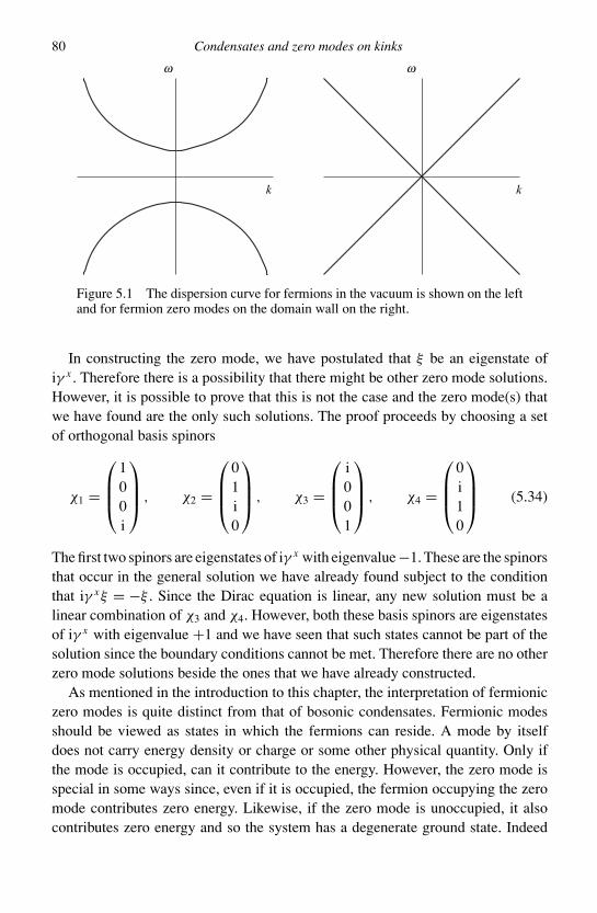
80 Condensates and zero modes on kinks
w w
k k
Figure 5.1 The dispersion curve for fermions in the vacuum is shown on the leftand for fermion zero modes on the domain wall on the right.
In constructing the zero mode, we have postulated that ξ be an eigenstate ofiγ x . Therefore there is a possibility that there might be other zero mode solutions.However, it is possible to prove that this is not the case and the zero mode(s) thatwe have found are the only such solutions. The proof proceeds by choosing a setof orthogonal basis spinors
χ1 =
100i
, χ2 =
01i0
, χ3 =
i001
, χ4 =
0i10
(5.34)
The first two spinors are eigenstates of iγ x with eigenvalue −1. These are the spinorsthat occur in the general solution we have already found subject to the conditionthat iγ xξ = −ξ . Since the Dirac equation is linear, any new solution must be alinear combination of χ3 and χ4. However, both these basis spinors are eigenstatesof iγ x with eigenvalue +1 and we have seen that such states cannot be part of thesolution since the boundary conditions cannot be met. Therefore there are no otherzero mode solutions beside the ones that we have already constructed.
As mentioned in the introduction to this chapter, the interpretation of fermioniczero modes is quite distinct from that of bosonic condensates. Fermionic modesshould be viewed as states in which the fermions can reside. A mode by itselfdoes not carry energy density or charge or some other physical quantity. Only ifthe mode is occupied, can it contribute to the energy. However, the zero mode isspecial in some ways since, even if it is occupied, the fermion occupying the zeromode contributes zero energy. Likewise, if the zero mode is unoccupied, it alsocontributes zero energy and so the system has a degenerate ground state. Indeed

5.3 Fractional quantum numbers 81
the occurrence of a zero mode leads to some novel and important quantum fieldtheoretic consequences that we shall outline in Section 5.3.
In the discussion of fermion zero modes above we have considered only a Yukawainteraction between the fermion field and the field that makes up the domain wall.More generally, there can also be Majorana interactions. Zero modes of Majoranafermions on domain walls have been discussed in [147].
Just like scalar field condensates and fermionic zero modes on domain walls,there can also be gauge field (or spin-1) condensates. These arise when the modelhas broken gauge symmetries in addition to broken discrete symmetries. This isprecisely the situation in the SU (5) × Z2 model discussed in Chapter 2 and thekinks in the model have condensates of spin-1 fields as we describe in Section 5.5.
Finally we close this section by remarking that there are several mathematical“index theorems” that can be used to obtain information on the number of zeromodes on a soliton [176]. In the case of domain walls that we have been discussing,however, the index theorems do not lead to a useful result.
5.3 Fractional quantum numbers
To quantize a fermionic field we find all the modes (solutions of the Dirac equation)and then associate creation and annhilation operators with each of the modes.2 Thesame procedure may be followed in the presence of zero modes [83]. As discussedin the previous section, there is a single zero mode on the Z2 kink (in one spatialdimension), which is denoted by ψ0. Then the expansion of the field operator inmodes is
ψ = a0ψ0 +∑
p
[bpψp+ + d†
pψcp−]
(5.35)
The second term is the usual sum over the positive energy modes, ψp+, and fermion-number conjugates of the negative energy modes, ψc
p−.3 There is no sum over spinbecause there is no spin degree of freedom in one spatial dimension. The first termin Eq. (5.35) contains the zero mode, ψ0, and a0 is the operator associated withthis mode. The term may seem strange because the zero mode does not have acorresponding conjugated term. This is because ψc
0 = ψ0 and so the mode func-tions associated with a0 and its conjugate operator are identical. However, one stillhas the usual equal time anticommutation relations for the field and its canonicalmomentum
ψa(x), ψ†b(y) = δ(x − y)δab (5.36)
2 We work in one spatial dimension in this section and hence spinors have two components.3 That is, ψc
p− is the wavefunction of a hole in the Dirac sea that has momentum p.

82 Condensates and zero modes on kinks
while other anticommutators vanish. Using the expansion in terms of creation andannihilation operators this gives
a0, a0 = a†0, a†
0 = 0, a0, a†0 = 1 (5.37)
Since the Dirac Lagrangian in Eq. (5.14) is invariant if the fermion fields arerotated by a phase, the model has a conserved fermion number current. The Noethercurrent is given by ψγ µψ (µ = 0, 1). In the quantum theory the physical currentoperator needs to be normal ordered. This is equivalent to defining the fermionnumber operator as
Qf =∫
dx : j0 := 1
2
∫dx(ψ†
αψα − ψαψ†α) (5.38)
We can act by this operator on any state to determine the fermion number of thatstate. Let us denote the state with no positive energy particles and empty zero modeby |0; −〉 and the state with no positive energy particles and filled zero mode by|0; +〉. Then the fermion numbers of these two states are
Qf|0; ±〉 = 1
2[a†
0a0 − a0a†0]|0; ±〉
= 1
2[2a†
0a0 − 1]|0; ±〉
= ±1
2|0; ±〉 (5.39)
Therefore the kink carries a half-integer fermion number of either sign. If thefermion carries electric charge, the electric charge on the kink is also half-integral.
It is critical to not think of the kink as being “kink plus fermion.” Instead the kinkis made of both the bosonic and fermionic fields. Then there are only two states forthe kink: one with filled zero mode and the second with the zero mode empty.
Surprising as the half-integer fermion number is, further work in [150, 68] ob-tained different fractional charges in other systems (see Section 9.1). Indeed, [68]shows that the charges can even be irrational.
5.4 Other consequences
If the bosonic condensate is electrically charged, the domain wall becomes super-conducting. To see this in some more detail, consider the case of a complex, elec-trically charged, scalar field, χ , interacting with the field φ that forms a domainwall
L = L[φ] + L[Aµ] + 1
2|Dµχ |2 − m2
χ
2|χ |2 − λχ
4|χ |4 − σ
2φ2|χ |2 (5.40)
5.4 Other consequences 83
The first term is the Lagrangian for the Z2 model and the second is the usualMaxwell Lagrangian for the gauge field Aµ. The covariant derivative is defined by
Dµ = ∂µ − iq Aµ (5.41)
The propagating modes of the condensate are
χ = χ0(x)ei(ωt−k·x) (5.42)
where χ0(x) is the condensate profile and k is the wave-vector restricted to lie inthe plane of the wall, the yz-plane. Since χ carries electric charge, q, the electriccurrent is
jχ = iq
2(χ †∇χ − χ∇χ †) (5.43)
Inserting Eq. (5.42) into (5.43), we find that the current is along the k direction
jχ = q|χ0|2k (5.44)
The simplest way to see that the wall with the condensate is superconducting isto write
χ = χ0(x)eiθ (5.45)
where χ0 is the condensate solution and θ is the phase variable. Then the lowenergy Lagrangian for the θ degree of freedom can be derived by integrating thefull Lagrangian density, Eq. (5.40), over x to get
L(θ ) = 1
2(∂µθ − eAµ)2 (5.46)
where we have omitted an overall constant factor. This effective Lagrangian isthe relativistic generalization of the Lagrangian in the Ginzburg-Landau theory ofsuperconductivity. Assuming that the relativistic generalization does not make anyqualitative difference, results from the Ginzburg-Landau theory can then be applieddirectly to the present case. In particular, the domain wall with charged condensatecan be expected to carry persistent electric currents, have magnetic vortices, andexhibit the Meissner effect (expulsion of magnetic fields) [61].
We now discuss fermionic superconductivity on domain walls. The relevantmodes are given in Eq. (5.33) and the (normal ordered) current is
jψ = q : ψ†γψ : (5.47)
Using the expansion of ψ in terms of creation and annihilation operators(Eq. (5.35)), the current in any Fock state of fermions can be evaluated. Similarly,the electric charge on a domain wall can also be evaluated.
Fermions on domain walls can only make the wall superconducting if they formCooper pairs and condense. It is believed that the slightest attractive interaction

84 Condensates and zero modes on kinks
between the fermions on the wall will lead to condensation below some criticaltemperature. On a domain wall, there are possible channels for attractive inter-actions. For example, the fermions interact with each other via exchange of φ
quanta and this can lead to an attractive force. The problem of rigorously showingfermionic superconductivity of domain walls has not been investigated. In partic-ular, the Meissner effect, which is the hallmark of superconductivity, has not beenshown. Indeed, the response of non-interacting fermion zero modes to an externalmagnetic field has been discussed with the conclusion that the walls are diamagnetic[173] (also see [82, 172]).
In the particle-physics/cosmology literature, the existence of electrically chargedzero modes is simply assumed to imply superconductivity (though see [15]). Areason for this assumption is that a current on a wall persists even without theapplication of an external electric field. Once the current carrying fermionic zeromode states have been populated there are very few processes by which these statescan be emptied [184]. Two such dissipative processes are the scattering of counter-propagating fermion zero modes, and the scattering of fermion zero modes withfluctuations of the domain wall field itself. Generally these processes occur at a veryslow rate, at least in astrophysical situations of interest. Hence, strictly speaking,domain walls in particle physics/cosmology have only been shown to be excellentconductors and not superconductors.
The equilibrium current on a domain wall in any setting depends on the balanceof the rates of current increase owing to an external electric field and decreaseowing to dissipation. Note that an external magnetic field in which a domain wall ismoving is, effectively, an electric field in the rest frame of the wall. Since magneticfields are ubiquitous in astrophysics, any cosmological domain walls with fermionzero modes can be expected to be current carrying. Superconducting domain wallsin realistic grand unification models have been discussed in [98].
The fermion zero mode states that we have discussed above are single particleeigenstates. The true states of the domain wall are also affected by fermion-fermioninteractions. The many-body problem falls in the class of two-dimensional systemsof interacting fermions. In the presence of a strong external magnetic field, so thatthe Landau level spacing is large compared to other energy scales, the fermions onthe wall are similar to electrons in a quantum Hall system.
5.5 Condensates on SU (5) × Z2 kinks
In Chapter 2 we have discussed kinks in an SU (5) × Z2 model, which is the simplestexample of a Grand Unified Theory. Even though SU (5) grand unification is knownnot to be phenomenologically viable, the model is still pedagogically useful.
5.5 Condensates on SU (5) × Z2 kinks 85
The Lagrangian for the model is
L = Lb[, χ, Xµ] + L f[χ, ψ, Xµ] (5.48)
where the SU (5) adjoint field, , does not couple directly to the fermionic fields(denoted generically by ψ). Only an additional SU (5) fundamental field, χ , couplesto the fermions. The vacuum expectation value of χ is responsible for electroweaksymmetry breaking and the masses of all the observed quarks and leptons arisefrom this symmetry breaking. The SU (5) symmetry breaking has no consequencesfor the fermionic sector, except via the χ field. This indirect effect can be importantin the presence of kinks, since χ can form a condensate on the kink, which can theninteract with some of the fermions. We will discuss this further below.
The bosonic part of the Lagrangian is
Lb = Tr(Dµ)2 + |Dµχ |2 − V (, χ ) − 1
2Tr(Xµν Xµν) (5.49)
The covariant derivative is defined by Dµ ≡ ∂µ − igXµ and its action on the scalarfields is
Dµ ≡ ∂µ − ig[Xµ, ], Dµχ ≡ (∂µ − igXµ)χ (5.50)
The potential is given by
V (, χ ) = V () + V (χ ) + λ4(Tr2)χ †χ + λ5(χ †2χ ) (5.51)
with
V () = −m21(Tr2) + λ1(Tr2)2 + λ2(Tr4) (5.52)
V (χ) = −m22χ
†χ + λ3(χ †χ )2 (5.53)
Successful grand unification requires that the global minimum of the potentialleaves an SU (3) × U (1) symmetry unbroken.4 As already described in Section 2.2,the minimum of the potential with χ set equal to zero, occurs at
0 = η
2√
15diag(2, 2, 2, −3, −3) (5.54)
(up to SU (5) × Z2 transformations) in the parameter range
λ ≥ 0, λ′ ≡ h + 7
30λ ≥ 0 (5.55)
The vacuum expectation value of breaks SU (5) × Z2 to [SU (3) × SU (2) ×U (1)]/Z6. If we assume that the back-reaction of a vacuum expectation value of χ
4 Symmetry breaking patterns have been discussed quite generally in [99].
86 Condensates and zero modes on kinks
on that of is small, we can write down a reduced potential for χ alone
Vred(χ ; 0) =(
−m22 + λ4Tr2
0 + λ5
15η2
)χ †
aχa
+(
−m22 + λ4Tr2
0 + 3λ5
20η2
)χ†bχb + λ3(χ †χ)2 (5.56)
where a = 1, 2, 3 and b = 4, 5. The symmetry is broken to [SU (3) × U (1)]/Z3
only if the vacuum expectation value of χ is along the χ4 or χ5 directions. Thisfurther restricts the range of parameters to
λ5
15η2 > m2
2 − λ4Tr20 >
3λ5
20η2, λ3 > 0 (5.57)
which also implies λ5 < 0 and m2 < λ4Tr20. We assume that these conditions on
the parameters are satisfied. Then a minimum of the reduced potential occurs at
χT = ηew(0, 0, 0, 1, 0) (5.58)
where
η2ew = 1
2λ3
(m2
2 − λ4Tr20 − 3λ5
20η2
)(5.59)
is the electroweak symmetry breaking scale. The final [SU (3) × U (1)]/Z3 sym-metry corresponds to the color and electromagnetic symmetries present today.
Next we describe the fermionic sector.5 There are two fermion fields: ψ , whichis in the fundamental (5-dimensional) representation of SU (5) and ζ , which is inthe antisymmetric 10-dimensional representation. The known quarks and leptonsfit within the components of these fields. With the choice of vacuum expectationvalues in Eq. (5.58)
(ψ i )L = (dc1, dc2, dc3, e−, −νe)L (5.60)
(ψ i )R = (d1, d2, d3, e+, −νce
)R (5.61)
(ζi j )L = 1√2
0 uc3 −uc2 u1 d1
−uc3 0 uc1 u2 d2
uc2 −uc1 0 u3 d3
−u1 −u2 −u3 0 e+
−d1 −d2 −d3 −e+ 0
L
(5.62)
(see Eq. (14.9) in [30]). The numerical index on the u and d fields refers to colorcharge, and the placement (subscript or superscript) depends on the representation
5 Actually we describe only one of the three families of the standard model fermionic sector, and then too theneutrino is taken to be massless.
5.5 Condensates on SU (5) × Z2 kinks 87
(fundamental or fundamental conjugate) in which the field transforms under theunbroken SU (3). The c superscript denotes charge conjugation:
ψc ≡ iγ 2ψ∗ (5.63)
The L and R subscripts refer to left- and right-handed spinors
ψL ≡ 1 − γ 5
2ψ, ψR ≡ 1 + γ 5
2ψ (5.64)
The Dirac γ matrices are defined in Eqs. (5.15) and (5.17).Now we are ready to describe the interactions of the various fields with the
SU (5) × Z2 kink, described as the q = 2 kink in Chapter 2.
In the presence of a (q = 2) kink, the vacuum expectation values are
(−∞) = + η
2√
15diag(2, 2, 2, −3, −3)
χT (−∞) = ηew(0, 0, 0, 1, 0)
(+∞) = − η
2√
15diag(2, −3, −3, 2, 2)
χT (+∞) = ηew(0, 0, 1, 0, 0)
Note that the non-trivial entry of χ has to coincide with one of the −3 entries of since this is what minimizes the potential V (, χ ). Therefore χ must rotatethrough the kink. Inside the kink, the fields are not pure rotations of the asymptoticvalues.
The component 11 goes from +2 to −2 as the wall is crossed. Hence it mustvanish in the wall. This is very similar to the Z2 case, where the field vanishesat the center of the wall. The field χ interacts with as given by the potentialin Eq. (5.51). Note the interaction term λ5Tr(χ †2χ ), which directly couples χ1
to 11. (The other term couples all components of χ to Tr2 only.) By explicitconstruction it can be seen that χ1 can condense on the wall for a certain rangeof parameters [146]. Hence the SU (5) × Z2 model allows for scalar condensateson the wall (see Section 5.1). In addition, since χ1 is a complex scalar field, thecondensate has an associated phase. The choice of phase on different parts of thewall may be different, leading to vortices in χ1 that can only exist on the wall.Since χ1 transforms non-trivially under the unbroken SU (3), the vortices carrycolor magnetic field. This is similar to our discussion below Eq. (5.46).
Next we consider fermion interactions with the wall [146]. The fermions do notcouple directly to . Hence the only coupling to the wall is due to the rotation of χ
in passage through the wall and to the condensate in the χ1 component. Considerthe scattering of the fifth component, ψ5, which corresponds to a neutrino on theleft side of the wall but a d-quark on the right. This fifth component has non-zero
88 Condensates and zero modes on kinks
reflection and transmission probability. If it reflects, the particle is still a neutrino.If it transmits, it must change into a d-quark. If a neutrino becomes a d-quark inpassing through the wall, it must pick up electric and color charge from the wall.Hence we are forced to conclude that there must be electric and color excitationsthat live entirely on the wall. If a χ1 condensate is not present, the only availableexcitations are the charged gauge field components. Hence charged gauge fieldsmust condense on the wall.
To see the presence of a charged gauge field condensate, it is most convenientto go to a gauge where the scalar field vacuum expectation values are oriented inthe same directions on both sides of the wall, as we now discuss.
Consider a very thin wall, so that
(x < 0) = + η
2√
15diag(2, 2, 2, −3, −3) ≡ 0
(x > 0) = − η
2√
15diag(2, −3, −3, 2, 2) (5.65)
Now we perform a local gauge transformation that rotates into the direction of0 (up to a sign) everywhere. Such a gauge rotation is local since it is equal to theidentity transformation for x < 0 but is non-trivial for x > 0 since it exchangesthe 23- and 45-blocks of . In both regions, x < 0 and x > 0, the gauge rotationis constant. The rotation is non-constant only at x = 0 i.e. on the wall. Hence thegauge fields after the rotation vanish everywhere except on the wall itself and thereare gauge degrees of freedom residing on the wall. A more explicit calculationshows that the gauge fields living on the wall carry electric and color charge.
5.6 Possibility of fermion bound states
In addition to fermionic zero modes on a kink, there may also be fermionic boundstates. Such bound states would have a non-vanishing energy eigenvalue ω with0 < ω < m. Since the energy eigenvalue is less than the asymptotic mass, thefermion would be bound to the wall. We examine whether the model in Eq. (5.14)leads to fermionic bound states on a Z2 kink.
For convenience we work in one spatial dimension. Then spinors have twocomponents and there are only two gamma matrices, which can be taken to be
γ 0 = σ 3 =(
1 00 −1
), γ 1 = iσ 1 =
(0 11 0
)(5.66)
Then the Dirac equation i∂ψ − gφkψ = 0 together with ψ = exp(−iωt)ξ gives
∂xξ1 = −(ω + gφk)ξ2
∂xξ2 = +(ω − gφk)ξ1 (5.67)

5.7 Open questions 89
where
ξ =(
ξ1(x)ξ2(x)
)(5.68)
and we are interested in solutions with
0 < ω < mf ≡ gη (5.69)
The boundary conditions at the origin for ξ1 and ξ2 may be determined bynoting that we are free to rescale both ξ1 and ξ2 by a constant factor. So we canset ξ1(0) = +1. Further, using the symmetry φk(x) = −φk(−x), we find that theequations are invariant if we replace ξ1(x) by cξ2(−x) and ξ2(x) by cξ1(−x), wherec is a constant. Hence
ξ1(x) = cξ2(−x), ξ2(x) = cξ1(−x) (5.70)
This gives
ξ1(x) = cξ2(−x) = c2ξ1(x) (5.71)
Since ξ1(x) cannot vanish for all x , we get
c = ±1 (5.72)
Therefore there are two possible boundary conditions at the origin
ξ2(0) = ±ξ1(0) = ±1 (5.73)
At infinity we require ξ1 → 0 and ξ2 → 0.A numerical search for a solution with non-zero ω did not reveal any bound
states for the range of parameters 0.1 < mfw < 20, where w is the width of thekink. However this does not exclude the existence of fermion bound states (besidethe zero mode) on kinks in other systems, and it remains an open problem to findsystems where such bound states exist.
5.7 Open questions
1. Explore the classical and quantum physics of a domain wall with electrically chargedbosonic and fermionic zero modes placed in an external magnetic field. What happensif the domain wall is moving?
2. Calculate the reflection of photons off a superconducting domain wall. Is the wall a goodmirror? (See [184].)
3. Construct a system in which the kink has both a zero mode and a fermionic bound state.
6
Formation of kinks
In this chapter we study the formation of kinks and domain walls during a phasetransition. We start by describing the effective potential for a field theory at finitetemperature. This sets up a useful framework for discussing phase transitions anddefect formation.
6.1 Effective potential
The effective potential is a tool that is often used to study phase transitions infield theory [89, 179, 90, 47, 100]. The idea is to consider the interaction ofa scalar degree of freedom (“order parameter”) with a thermal background ofparticles. Such processes induce additional temperature dependent terms in thepotential for the order parameter, leading to an “effective potential.” The shapeof the effective potential varies as a function of temperature and new minimamight appear. The global minimum defines the vacuum of the model. If a newglobal minimum appears at some temperature, it indicates that the system makesa transition to a new expectation value of the order parameter and there is aphase change. We now describe the (one loop) effective potential in a little moredetail.
We consider a field theory of scalar, spinor and vector fields
L = LB + LF (6.1)
with the bosonic Lagrangian
LB = 1
2(Dµi )D
µi − V () − 1
4Fa
µν Fµνa (6.2)
where i are the components of the scalar fields,
Dµ ≡ ∂µ − ieAaµT a (6.3)
90
6.1 Effective potential 91
the T a are group generators, and
Faµν ≡ ∂µ Aa
ν − ∂ν Aaµ + e f abc Ab
µ Acν (6.4)
where Aaµ are the gauge fields.
The Lagrangian for a fermionic multiplet is
LF = iγ µDµ − ii (6.5)
where i are the Yukawa coupling matrices. The quantity denotes a collection offermionic fields and the Yukawa coupling term may be written more explicitly asσ
α αβ
iσρρβ i where α, β label the various fermionic fields, the superscripts σ, ρ
on the fermion fields are spinor indices, and i labels the interaction term with thescalar field i . i has spinor indices because it could contain the unit matrix (vectorcoupling) and/or the γ 5 matrix (axial coupling) defined in Eq. (5.17).
If the expectation values of the scalar fields are denoted by 0i , then the massmatrices of the various fields are written as
µ2i j = ∂2V
∂i∂ j
∣∣∣∣=0
, scalar fields (6.6)
m = i0i , spinor fields (6.7)
M2ab = e2(TaTb)i j0i0 j , vector fields (6.8)
where a, b are gauge field group indices.Then the finite temperature, one loop effective potential is1
Veff(0, T ) = V (0) + M2
24T 2 − π2
90N T 4 (6.9)
where
N = NB + 7
8NF (6.10)
is the number of bosonic and fermionic spin states, and
M2 = Tr(µ2) + 3Tr(M2) + 1
2Tr(γ 0mγ 0m) (6.11)
where γ 0 is defined in Eq. (5.15). Note that M2 depends on the expectation value0 through the defining equations for the mass matrices given above. For example,M2 contains a term proportional to Tr(2
0).An important feature of the effective potential is that it can show the presence
of phase transitions. If there are scalar fields with negative mass squared terms in
1 Radiative corrections and spontaneous symmetry breaking are discussed in [33, 178].
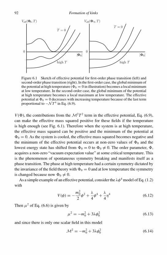
92 Formation of kinks
|Φ0|
Veff(Φ
0, T )
T = 0
high T
0|Φ0|
Veff(Φ 0, T )
T = 0
high T
0
Figure 6.1 Sketch of effective potential for first-order phase transition (left) andsecond-order phase transition (right). In the first-order case, the global minimum ofthe potential at high temperature (0 = 0 in illustration) becomes a local minimumat low temperature. In the second-order case, the global minimum of the potentialat high temperature becomes a local maximum at low temperature. The effectivepotential at 0 = 0 decreases with increasing temperature because of the last termproportional to −N T 4 in Eq. (6.9).
V (), the contributions from the M2T 2 term in the effective potential, Eq. (6.9),can make the effective mass squared positive for these fields if the temperatureis high enough (see Fig. 6.1). Therefore when the system is at high temperature,the effective mass squared can be positive and the minimum of the potential at0 = 0. As the system is cooled, the effective mass squared becomes negative andthe minimum of the effective potential occurs at non-zero values of 0 and thelowest energy state has shifted from 0 = 0 to 0 = 0. The order parameter, ,acquires a non-zero “vacuum expectation value” at some critical temperature. Thisis the phenomenon of spontaneous symmetry breaking and manifests itself as aphase transition. The phase at high temperature had a certain symmetry dictated bythe invariance of the field theory with 0 = 0 and at low temperature the symmetryis changed because now 0 = 0.
As a simple example of an effective potential, consider the λφ4 model of Eq. (1.2)with
V (φ) = −m20
2φ2 + λ
4φ4 + λ
4η4 (6.12)
Then µ2 of Eq. (6.6) is given by
µ2 = −m20 + 3λφ2
0 (6.13)
and since there is only one scalar field in this model
M2 = −m20 + 3λφ2
0 (6.14)

6.2 Phase dynamics 93
Therefore, up to a term that is independent of φ0, the effective potential becomes
Veff(φ0, T ) = m2
2φ2
0 + λ
4φ4
0 (6.15)
with
m2 = −m20 + λ
4T 2 (6.16)
Note that the masses of small excitations around the true vacuum are given byV ′′
eff(φ0) withφ0 being the vacuum expectation value. By minimizing Veff (Eq. (6.15))we get
φ0,min(T ) = 0, m2 > 0 (6.17)
=√
−m2
λ, m2 < 0 (6.18)
leading to the mass squared for small excitations (particles) in the true vacuum
m2eff ≡ V ′′
eff(φ0,min) = λ
4
(T 2 − T 2
c
), T > Tc (6.19)
= λ
2
(T 2
c − T 2), T < Tc (6.20)
where Tc is the critical temperature
Tc = 2m0√λ
(6.21)
In cosmology, since the universe is expanding, it is also cooling. Thereforewe can have one or many cosmological phase transitions and the particle-physicssymmetries at high temperatures (early universe) and low temperatures (recentuniverse) are different. The symmetry after the phase transition can be smalleror larger than the symmetry before the phase transition. In other words, loweringthe temperature can spontaneously break or restore a symmetry. We will mostlyconsider symmetry breaking during the phase transition but examples of symmetryrestoration are also easy to construct. A system in which symmetry restoration isobserved is Rochelle salt [85, 179].
6.2 Phase dynamics
The effective potential Veff(0, T ) is calculated for a system that is in thermal equi-librium, assuming a homogeneous vacuum expectation value of the order parameter0. Yet thermal equilibrium is not maintained during the phase transition and alsothe phase change occurs in an inhomogeneous manner. The dynamics are clear

94 Formation of kinks
Figure 6.2 A schematic diagram of bubbles nucleating in a first-order phasetransition. The two types of bubbles correspond to the two different values of theorder parameter. The bubbles grow and collide, and new bubbles nucleate as well.Eventually the whole system is in the new phase.
for a first-order phase transition in which the high temperature phase becomes ametastable state (see Fig. 6.1) at some critical temperature. Now the system can bestuck in this metastable state even when the temperature drops significantly belowthe critical temperature. An external perturbation can cause the system to transitionto the global vacuum. In the absence of an external perturbation, quantum tunnelingcan trigger the transition. In either case, bubbles of a critical size of the true vacua(0 = 0) nucleate in the false vacuum (0 = 0) background (see Fig. 6.2). Thesebubbles grow and eventually merge thus filling space and completing the phasetransition. Clearly this process is not homogeneous and cannot be described by aneffective potential.
In a second-order transition, in contrast to a first-order transition, there is nometastable state in which the system can be trapped. Thus 0 evolves continuously(“spinodal decomposition”) from 0 = 0 to 0 = 0. However, different spatialregions evolve at different rates owing to thermal and quantum fluctuations, and 0
is not spatially uniform. Once again, since the effective potential assumes constant0, it can indicate the existence of a second-order phase transition but cannotbe expected to accurately describe the dynamics of the transition. Since defectformation crucially depends on the inhomogeneities of the order parameter duringthe transition, new ideas have been needed to predict the statistical properties ofdefects formed in a second-order phase transition.
In one spatial dimension, the distribution of kinks is described by the numberdensity of kinks, and correlators of kink locations. In higher dimensions, the prob-lem becomes richer because domain walls are extended and can curve and havecomplicated topology. In addition to the mass density in domain walls, we are
6.3 Kibble mechanism: first-order phase transition 95
interested in the statistical distribution of shapes and sizes of domain walls formedat the phase transition.
6.3 Kibble mechanism: first-order phase transition
At a first-order phase transition, the order parameter has to change from 0 = 0 toits non-zero vacuum expectation value. We are interested in the case when there ismore than one possible non-zero value for 0. Then the dynamics in a small spatialregion select a vacuum. However the vacuum selected in different spatial regionscan be different. For example, in the case of the Z2 model, the field in a certainregion might relax into the φ = +η vacuum, whereas in another region it mightrelax into φ = −η (see Fig. 6.2).
In a first-order phase transition, each bubble is filled with constant 0 i.e. afixed vacuum is chosen within a bubble but it can be different for different bubbles.With time, the bubbles grow and collide and fill up the volume. Let us denote byξ the characteristic size of a region where the same vacuum is selected, after thephase transition is over. Then ξ is the typical size of bubbles when they percolate.If denotes the bubble nucleation rate per unit volume and v is the velocity ofthe growing bubble walls, then we can define a length scale and a time scale ondimensional grounds (in D spatial dimensions) by
ξ =( v
)1/(D+1), τ =
(1
vD
)1/(D+1)
(6.22)
The domain size ξ is a numerical factor times ξ and in practice we take ξ ∼ ξ .Similarly τ is related to the time that it takes to complete the phase transition.2
The process of bubble percolation has been studied both analytically and nu-merically [95]. Taking the centers of the bubbles as the vertices of a lattice andconnecting only the centers of bubbles that collide, we obtain a random lattice (seeFig. 6.3). We would like to determine the characteristics of such a random latticesince this plays a role in determining the network of defects that form. For example,the typical number of bubbles with which any given bubble collides, also knownas the “coordination number” of the random lattice, plays a role in the fraction ofclosed topological defects (closed domain walls, loops of string, or closely pairedmonopole-antimonopole pair) that are formed.
In one spatial dimension, every bubble trivially collides with two other bubbles.In two spatial dimensions the average number of collisions is the same as thecoordination number of a fully triangulated lattice of infinite extent. From purely
2 Equation (6.22) relates ξ to the nucleation rate , but it is very hard to measure in any experiment. In fact, itmay be easier to measure properties of the defect network, then ξ , and from it infer .

96 Formation of kinks
Figure 6.3 If two bubbles collide, their centers are joined by straight lines. Thefigure then shows the “random bubble lattice” expected in a first-order phasetransition in two spatial dimensions.
geometrical constraints that we describe next, the coordination number is six (see,for example, [129]).
The lattice is infinite in extent and by identifying the points at infinity we canview the lattice as lying on a two-dimensional sphere. Then Euler’s formula relatesthe number of vertices (V ), edges (E) and faces (F) of the lattice
V − E + F = 2 (6.23)
Let the coordination number be n. Therefore for every vertex there are n edgesbut every edge is bounded by two vertices. This relates the number of edges to thenumber of vertices: E = nV/2. Also, every face is a triangle, giving three edgesto every face. But an edge is shared by two faces. So E = 3F/2. Putting togetherthese relations in Euler’s formula gives
V − nV/2 + nV/3 = 2 (6.24)
In the limit of V → ∞, this yields n = 6.In three spatial dimensions, similar arguments have been given [95] to show
that the average coordination number is 13.4. This result is not completely fixedby geometrical constraints as in two dimensions and the result can vary a littledepending on the details of the bubble size distribution.
Returning to the λφ4 model, each bubble either has the phase φ0 = +η or φ0 =−η within it. If bubbles of different phases collide, a domain wall forms between thecenters of those bubbles. If bubbles of the same phase collide, a wall does not form,though it is possible that a closed domain wall or a wall-antiwall pair forms owing
6.4 Correlation length 97
to the energetics of the bubble collision. We expect small closed walls and closelyseparated walls and antiwalls to annihilate. Hence the distribution of domain wallsafter the phase transition is simply described by the locations of bubble collisionswhen the bubbles carry different phases. Since the phase in the bubbles is ±η withequal probability, the phase transition is simulated by assigning ±η to each of thevertices of the random bubble lattice as in Fig. 6.3. We shall further discuss theproperties of the wall network at formation during a first-order phase transition inSection 6.6.
As we have seen, a first-order phase transition is relatively simple to conceptual-ize. A second-order phase transition is harder to understand. To discuss second-orderphase transitions, it is useful to first define an equilibrium correlation length.
6.4 Correlation length
The “equilibrium correlation length,” ξ , is defined as the distance over which fieldcorrelations are significant. Generally the field correlations at two spatial pointsfall off exponentially with increasing separation between the points, exp(−r/ξ ),and the exponent defines the equilibrium correlation length, ξ . Hence we need toevaluate the correlation function
G(r ) = 〈T |φ(t, x)φ(t, y)|T 〉 (6.25)
where G only depends on r ≡ |x − y|because the system is translationally invariant.The thermal state is denoted by |T 〉 and is defined as the state containing theequilibrium number density distribution (Fermi-Dirac or Bose-Einstein) of particles
|T 〉 = |nk〉T (6.26)
nk = 1
eβωk ± 1(6.27)
where β ≡ 1/T and ωk is the energy of particles in the k mode.3
With the Z2 model in mind, we have only one scalar field and the quantum fieldoperator can be expanded in modes about the true vacuum
φ(t, x) = φ0(T ) +∫
d3k
(2π )3
1√2ωk
[e−iωk t+ik·xak + e+iωk t−ik·xa†
k
](6.28)
where φ0(T ) is the vacuum expectation value of the field at temperature T , and ak
and a†k are annihilation and creation operators. The dispersion relation is that for
a free particle with temperature dependent mass m(T ) (see Eq. (6.20) for the λφ4
model; we have dropped the subscript “eff” for convenience)
ω2k = k2 + m2 (6.29)
3 The chemical potential vanishes in the present case.
98 Formation of kinks
The thermal state |T 〉 contains a Bose-Einstein distribution of the particle exci-tations and the number of scalar particles at momentum k is given by
nk = 1
eβωk − 1(6.30)
where β = 1/T (Boltzmann constant has been set to 1).By inserting the expansion in Eq. (6.28) in the correlator, we find
G(r ) =∫
d3k
(2π )3
1√2ωk
∫d3 p
(2π )3
1√2ωp
ei(k·x−p·y)〈T |a†kap|T 〉 + K (6.31)
where K is a constant which is independent of temperature and proportional toδ(3)(x − y). Then
G(r ) =∫
d3k
(2π )3
e−ik·(x−y)
eβωk − 1+ K
= T
4πre−m(T )r + K (6.32)
where, in doing the integral, we have assumed m(T ) T . From the final expressionwe get the equilibrium correlation length
ξ = 1
m(T )(6.33)
For the Z2 model (Eq. (6.20))
m2 = λ
4
(T 2 − T 2
c
), T > Tc (6.34)
= λ
2
(T 2
c − T 2), T < Tc (6.35)
Therefore the equilibrium correlation length is
ξ (T ) =√
4
λ
1√T 2 − T 2
c
, T > Tc (6.36)
=√
2
λ
1√T 2
c − T 2, T < Tc (6.37)
or
ξ (T ) ∝ |T − Tc|−1/2 (6.38)
The essential feature in ξ is the singularity at T = Tc, that occurs at a time thatwe denote tc. Assuming that the cooling (quench) occurs at a constant rate Tc/τext
(in a range of temperature around Tc), we have
T − Tc = − Tc
τext(t − tc) (6.39)

6.4 Correlation length 99
c
x
tt
Figure 6.4 Sketch of equilibrium correlation length as a function of time as givenin Eq. (6.40).
hence we write
ξ ∼ |T − Tc|−ν ∝ |t − tc|−ν (6.40)
for T close to Tc. The exponent ν is called a “critical exponent” and the meanfield theory calculation described above gives ν = 1/2. However, the mean fieldtheory ignores particle interactions and renormalization group methods give ν =2/3, which is closer to experiment. A sketch of the shape of ξ (Eq. (6.40)) is shownin Fig. 6.4.
One shortcoming of the mean field calculation of ξ is that we have quantizedthe field φ in a fixed true vacuum so that φ0(T ) in Eq. (6.28) is independent of x .This assumes that the same vacuum is chosen everywhere below Tc. On the otherhand, we are precisely interested in the spatial extent of a region in a single vacuum.Hence a more suitable expansion of φ would be
φ(t, x) = φ0(t, x, T ) +∫
d3k
(2π )3
1√2ωk
[fk(t, x)ak + f ∗
k (t, x)a†k
](6.41)
instead of Eq. (6.28). The vacuum expectation value, φ0, is now allowed to dependon both t and x since the background domain walls may be non-static. The secondterm in the expansion describes small fluctuations (particles) with mode functionsfk in the classical background φ0(t, x, T ) at x .
The expansion in Eq. (6.41) is not as obvious as might appear at first sight. Wehave seen in Chapter 4 that a kink can itself be written in terms of particles via theMandelstam operator. This was done in the sine-Gordon model but it is conceivablethat such an operator also exists in other models. So the above expansion only makessense for a state in which there is a clear separation between the particle degreesof freedom appearing in the sum and the soliton degrees of freedom included inφ0. For example, if the walls are very close to each other the separation of the two

100 Formation of kinks
terms may not be justified. Hence the phenomenon of defect formation is closelytied to the separation of classical (soliton) and quantum (particle) variables.
We are interested in
ξ0 = 〈T |φ0(t, x, T )φ0(t, y, T )|T 〉 (6.42)
However, we have no way of calculating this equal time “domain correlation func-tion” since (i) the thermal state refers to a thermal distribution of particles, not ofdomains, and (ii) the defects do not remain in thermal equilibrium with the par-ticles. This impasse is made less severe by realizing that the calculation of ξ forT > Tc does not suffer from this problem since then φ0 = 0 is the unique vacuum.We expect the correlations for T < Tc to be determined by those for T > Tc and soit might be sufficient to know the correlation length for T > Tc. (We discuss thisfurther in Section 6.5.) To emphasize this point, the two branches of the sketch inFig. 6.4 correspond to two different quantities – the equilibrium correlation lengthfor t < tc is for excitations in a different vacuum from that for t > tc. So, whileEq. (6.40) describes the correlations of particle excitations in a given true vacuumfor T < Tc (t > tc), we cannot expect that this has anything to do with the size ofdomains of constant vacuum.
The next subtlety is that the divergence of the equilibrium correlation length atT = Tc should not be taken too literally. The reason is that there is an externalagency (refrigerator) driving the phase transition on a time scale given by τext. Asthe system gets closer to the critical temperature, it takes longer for equilibriumto be established, while the external agency continues to cool the system at a ratedetermined by external factors. At some temperature above the critical temperaturethe time taken to maintain equilibrium becomes larger than the time scale at whichthe external conditions are changing.
Assume that the external temperature is being lowered at a constant rate
T = Tc
(1 − t
τext
)(6.43)
where Tc is the critical temperature and we have chosen Tc = 0 for convenience.The equilibrium correlation length has the form
ξ (T ) = η|ε|−ν (6.44)
where ν is a critical exponent, η is some unspecified length scale, and
ε ≡ 1 − T
Tc(6.45)
The rate of change of ξ is
dξ
dt= − ε
|ε|νη
τext|ε|−(ν+1) = − νξ
τextε(6.46)
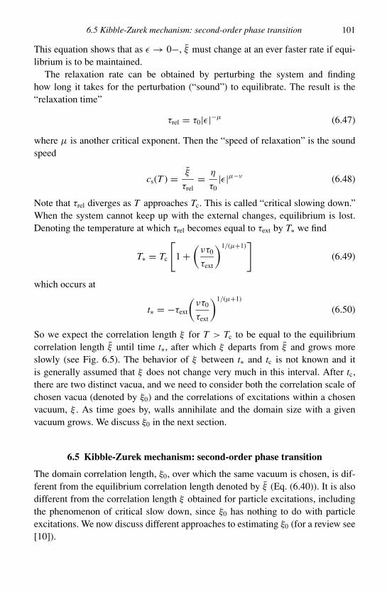
6.5 Kibble-Zurek mechanism: second-order phase transition 101
This equation shows that as ε → 0−, ξ must change at an ever faster rate if equi-librium is to be maintained.
The relaxation rate can be obtained by perturbing the system and findinghow long it takes for the perturbation (“sound”) to equilibrate. The result is the“relaxation time”
τrel = τ0|ε|−µ (6.47)
where µ is another critical exponent. Then the “speed of relaxation” is the soundspeed
cs(T ) = ξ
τrel= η
τ0|ε|µ−ν (6.48)
Note that τrel diverges as T approaches Tc. This is called “critical slowing down.”When the system cannot keep up with the external changes, equilibrium is lost.Denoting the temperature at which τrel becomes equal to τext by T∗ we find
T∗ = Tc
[1 +
(ντ0
τext
)1/(µ+1)]
(6.49)
which occurs at
t∗ = −τext
(ντ0
τext
)1/(µ+1)
(6.50)
So we expect the correlation length ξ for T > Tc to be equal to the equilibriumcorrelation length ξ until time t∗, after which ξ departs from ξ and grows moreslowly (see Fig. 6.5). The behavior of ξ between t∗ and tc is not known and itis generally assumed that ξ does not change very much in this interval. After tc,there are two distinct vacua, and we need to consider both the correlation scale ofchosen vacua (denoted by ξ0) and the correlations of excitations within a chosenvacuum, ξ . As time goes by, walls annihilate and the domain size with a givenvacuum grows. We discuss ξ0 in the next section.
6.5 Kibble-Zurek mechanism: second-order phase transition
The domain correlation length, ξ0, over which the same vacuum is chosen, is dif-ferent from the equilibrium correlation length denoted by ξ (Eq. (6.40)). It is alsodifferent from the correlation length ξ obtained for particle excitations, includingthe phenomenon of critical slow down, since ξ0 has nothing to do with particleexcitations. We now discuss different approaches to estimating ξ0 (for a review see[10]).
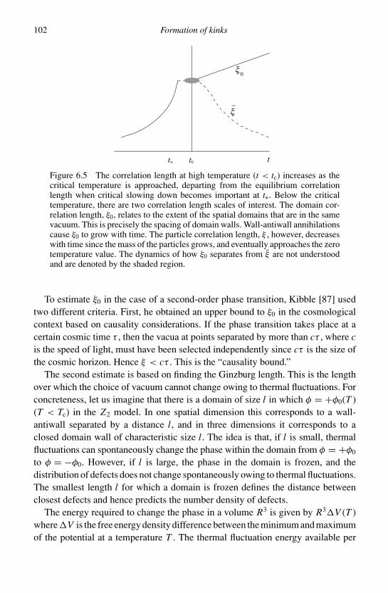
102 Formation of kinks
x
x0
t tc t*
Figure 6.5 The correlation length at high temperature (t < tc) increases as thecritical temperature is approached, departing from the equilibrium correlationlength when critical slowing down becomes important at t∗. Below the criticaltemperature, there are two correlation length scales of interest. The domain cor-relation length, ξ0, relates to the extent of the spatial domains that are in the samevacuum. This is precisely the spacing of domain walls. Wall-antiwall annihilationscause ξ0 to grow with time. The particle correlation length, ξ , however, decreaseswith time since the mass of the particles grows, and eventually approaches the zerotemperature value. The dynamics of how ξ0 separates from ξ are not understoodand are denoted by the shaded region.
To estimate ξ0 in the case of a second-order phase transition, Kibble [87] usedtwo different criteria. First, he obtained an upper bound to ξ0 in the cosmologicalcontext based on causality considerations. If the phase transition takes place at acertain cosmic time τ , then the vacua at points separated by more than cτ , where cis the speed of light, must have been selected independently since cτ is the size ofthe cosmic horizon. Hence ξ < cτ . This is the “causality bound.”
The second estimate is based on finding the Ginzburg length. This is the lengthover which the choice of vacuum cannot change owing to thermal fluctuations. Forconcreteness, let us imagine that there is a domain of size l in which φ = +φ0(T )(T < Tc) in the Z2 model. In one spatial dimension this corresponds to a wall-antiwall separated by a distance l, and in three dimensions it corresponds to aclosed domain wall of characteristic size l. The idea is that, if l is small, thermalfluctuations can spontaneously change the phase within the domain from φ = +φ0
to φ = −φ0. However, if l is large, the phase in the domain is frozen, and thedistribution of defects does not change spontaneously owing to thermal fluctuations.The smallest length l for which a domain is frozen defines the distance betweenclosest defects and hence predicts the number density of defects.
The energy required to change the phase in a volume R3 is given by R3V (T )whereV is the free energy density difference between the minimum and maximumof the potential at a temperature T . The thermal fluctuation energy available per
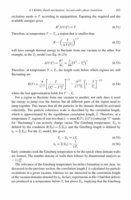
6.5 Kibble-Zurek mechanism: second-order phase transition 103
excitation mode is T according to equipartition. Equating the required and theavailable energies gives
R3V (T ) ≈ T (6.51)
Therefore, at temperature T < Tc, a region that is smaller than
R ∼(
T
V (T )
)1/3
(6.52)
will have enough thermal energy to fluctuate from one vacuum to the other. Forexample, in the Z2 model (see Eq. (6.15))
V (T ) = m4
4λ= λ
64
(T 2 − T 2
c
)2(6.53)
Therefore, at temperature T < Tc, the length scale below which regions are stillfluctuating are
R(T ) = 4
λ1/3
[T(
T 2c − T 2
)2]1/3
∼ 42/3
λ1/3Tc
[1 − T
Tc
]−2/3
(6.54)
where the last approximation holds for T ∼ Tc.For a region to fluctuate from one vacuum to another, not only does it need
the energy to jump over the barrier, but all different parts of the region need tojump together. This means that all the particles in the domain should be activatedcoherently. The particle coherence scale is described by the correlation length,which is approximated by the equilibrium correlation length, ξ . Therefore, at atemperature T , regions of size less than lf = min(R(T ), ξ (T )) (subscript “f” standsfor “fluctuating”) can actively change vacua. The Ginzburg temperature, TG, isdefined by the condition R(TG) = ξ (TG), and the Ginzburg length is defined bylG = ξ (TG). For the Z2 model, this gives
Tc − TG ≈ λTc (6.55)
lG = ξ (TG) ≈ 1
λTc(6.56)
Early estimates took the Ginzburg temperature to be the epoch when domain wallsare formed. The number density of walls then follows by dimensional analysis as∼ 1/ l D
G .The relevance of the Ginzburg temperature for defect formation is not clear. As
discussed in the previous section, the correlation length ξ is calculated for particleexcitations in a given vacuum, whereas we are interested in the correlation lengthof the vacuum domains denoted by ξ0. In fact, experiments in He-3 find that defectsare produced at a temperature below Tc but above TG, implying that the Ginzburg
104 Formation of kinks
criterion is not a necessary condition for defect formation. A discussion of therelevance of the Ginzburg criterion in the context of vortex formation in He-3 andHe-4 may be found in [86].
Zurek estimated the domain size, ξZ, by considering the time scales involvedduring the phase transition [187, 188, 93]. As discussed at the end of Section 6.4, thesystem cannot keep up with external changes at t = t∗ (Fig. 6.5). Zurek postulatedthat the correlation length at the instant when the system can no longer keep upwith the external changes determines the size of the domains that get frozen. Thisin turn determines the number of defects.
To estimate ξ0 at tc we know ξ at the time critical slowing down becomes im-portant. To this we add the distance that a perturbation can propagate from theslow-down time, t∗, to the phase transition time, tc (see Fig. 6.5). That gives us
ξ0(tc) = ξ (t∗) +∫ tc
t∗dt cs(t) (6.57)
= η1 + µ
1 + µ − ν
(τext
ντ0
)ν/(1+µ)
(6.58)
The crucial part of this relation is
ξ0(tc) ∝(
τext
τ0
)ν/(1+µ)
(6.59)
This relation gives the dependence of the number density of domain walls in Dspatial dimensions on the external time
n ∝(
τext
τ0
)−νD/(1+µ)
(6.60)
We can control τext in experiments and hence this is a testable prediction.The above analysis can be improved yet further. For example, we have calculated
ξ0 at t = tc. Yet thermal fluctuations after t = tc (i.e. T < Tc) may be important andthe domain structure may freeze out at yet lower temperatures, as in the discussionof the Ginzburg length scale above. So the relevant time at which ξ0 is stable tothermal fluctuations is somewhat after tc, in agreement with the analysis of [8].
There is yet another view of defect formation at a phase transition first proposedin [5]. In numerical simulations of a U (1) field theory, the authors found thatthere is a distribution of vortices even at temperatures above the phase transition.However, these vortices are small, closed structures. At the critical temperature,the vortices link up and form infinite, open structures. Thus the phase transition iscoincident with a percolation transition of the vortices. If this feature is generallytrue, we expect a population of small, closed domain walls to exist above the criticaltemperature. As the temperature is lowered, the walls connect and grow larger and
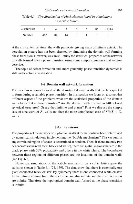
6.6 Domain wall network formation 105
Table 6.1 Size distribution of black clusters found by simulationson a cubic lattice.
Cluster size 1 2 3 4 6 10 31 082
Number 462 84 14 13 1 1 1
at the critical temperature, the walls percolate, giving walls of infinite extent. Thepercolation picture has not been checked by simulating the domain wall formingphase transition. However, we can still study the statistical properties of the networkof walls formed after a phase transition using some simple arguments that we nowdescribe.
The topic of defect formation and, more generally, phase transition dynamics isstill under active investigation.
6.6 Domain wall network formation
The previous sections focused on the density of domain walls that can be expectedto form during a suitable phase transition. In this section we focus on a somewhatdifferent aspect of the problem: what are the statistical properties of the domainwalls formed at a phase transition? Are the domain walls formed as little closedspherical structures? Or are they infinite and planar? First we discuss the simplecase of a network of Z2 walls and then the more complicated case of SU (5) × Z2
walls.
6.6.1 Z2 network
The properties of the network of Z2 domain walls at formation have been determinedby numerical simulations implementing the “Kibble mechanism.” The vacuum inany correlated region of space is determined at random. Then, if there are only twodegenerate vacua (call them black and white), there are spatial regions that are in theblack phase with 50% probability and others in the white phase. The boundariesbetween these regions of different phases are the locations of the domain walls(see Fig. 6.6).
Numerical simulations of the Kibble mechanism on a cubic lattice gave thestatistics shown in Table 6.1 [74, 159]. The data show that there is essentially onegiant connected black cluster. By symmetry there is one connected white cluster.In the infinite volume limit, these clusters are also infinite and their surface areasare infinite. Therefore the topological domain wall formed at the phase transitionis infinite.

106 Formation of kinks
Figure 6.6 The distribution of two phases (black and white) on a square latticein two spatial dimensions. Domain walls lie at the interface of the black and whiteregions.
6.6.2 SU (5) network
What does the Kibble mechanism predict for SU (5) × Z2 domain walls? Just as inthe Z2 case, we have to throw down values of the Higgs field on a lattice, assumingthat every point on the vacuum manifold is equally likely, and then examine thewalls that would form at the interface. In Section 2.2 we have found that there arethree kinds of wall solutions in this model and we have labeled the walls by theindex q , which can take values 0, 1, or 2. Each kind of wall has the same topologybut they have different masses. Each wall type is formed with some probability.Based on the Kibble mechanism, the probability that a certain wall forms is directlyrelated to the number of boundary values that result in the formation of that kind ofwall. So we need to evaluate all the boundary conditions that lead to domain wallswith a certain value of q.
The space of boundary conditions leading to a given type of domain wall isdiscussed in Section 2.4. However, similar considerations occur in simpler modelsand it is helpful to think of the problem in a discrete case, for example the S5 × Z2
kinks described in Section 2.5. Take a fixed (discrete) vacuum in one domain. Theneighboring domain can be in any other vacuum state with equal probability.There are ten possible states for the neighboring domain. Only one of these givesthe q = 0 wall, six give the q = 1 wall, and three give the q = 2 wall. Then theKibble mechanism implies that the network contains q = 0, 1, 2 walls and theirnumber densities are in the ratio 1 : 6 : 3. This means that the network is domi-nantly composed of the q = 1 wall. However, since the q = 2 wall is the lightestwall, the q = 1 walls formed by the Kibble mechanism during the phase transi-tion subsequently decay into q = 2 walls. We will show some evidence for thistwo-stage process in Section 6.7.
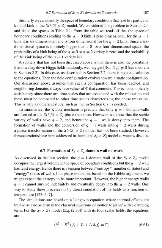
6.7 Formation of S5 × Z2 domain wall network 107
Similarly we can identify the space of boundary conditions that lead to a particularkind of kink in the SU (5) × Z2 model. We considered this problem in Section 2.4and listed the spaces in Table 2.1. From the table we read off that the space ofboundary conditions leading to the q = 0 kink is zero dimensional, for the q = 1kink it is six dimensional, and is four dimensional for the q = 2 kink. Since a six-dimensional space is infinitely bigger than a 0- or a four-dimensional space, theprobability of a kink being of the q = 0 or q = 2 variety is zero, and the probabilityof the kink being of the q = 1 variety is 1.
A subtlety that has not been discussed above is that there is also the possibilitythat if we lay down Higgs fields randomly, we may get [−, +] = 0 (see theoremin Section 2.2). In this case, as described in Section 2.2, there is no static solutionto the equations. Then the field configuration evolves toward a static configuration.Our discussion above assumes that such a configuration has been reached, andneighboring domains always have values of that commute. This is not completelysatisfactory since there are time scales that are associated with the relaxation andthese must be compared to other time scales characterizing the phase transition.This is why a numerical study, such as that in Section 6.7, is needed.
To summarize, the Kibble mechanism predicts that only q = 1 domain wallsare formed at the SU (5) × Z2 phase transition. However, we know that the stablevariety of walls have q = 2, and hence the q = 1 walls decay into them. Theformation of walls and the conversion of q = 1 walls into q = 2 walls duringa phase transformation in the SU (5) × Z2 model has not been studied. However,these questions have been addressed in the related S5 × Z2 model as we now discuss.
6.7 Formation of S5 × Z2 domain wall network
As discussed in the last section, the q = 1 domain wall of the S5 × Z2 modeloccupies the largest volume in the space of boundary conditions but the q = 2 wallhas least energy. Hence there is a tension between “entropy” (number of states) and“energy” (mass of wall). In a phase transition, based on the Kibble argument, wemight expect the entropy to be more important. However, the higher energy wallsq = 1 cannot survive indefinitely and eventually decay into the q = 2 walls. Oneway to study these processes is by direct simulation of the fields as a function oftemperature [123, 6, 7].
The simulations are based on a Langevin equation where thermal effects aretreated as a noise term in the classical equations of motion together with a dampingterm. For the S5 × Z2 model (Eq. (2.30)) with its four scalar fields, the equationsare (
∂2t − ∇2
)fi + Vi + ∂t fi = i (6.61)

108 Formation of kinks
0 50 100 150 200 2500
5
10
15
E,t
= 3
50.
0 50 100 150 200 2500
2
4
x 10−3
E,t
= 5
95.
0 50 100 150 200 2500
2
4x 10
−3
E,t
= 7
00.
0 50 100 150 200 2500
2
4x 10
−3
x
E,t
= 2
800.
Figure 6.7 Energy density distribution in space at an early time at high temper-ature (top panel) and then at various times after the phase transition in the lowerpanels. The last panel shows that the system has relaxed into a stable lattice ofkinks.
where i = 1, . . . , 4 and Vi denotes the derivative of V with respect to fi . If =0 = i , these equations are simply the classical equations of motion for the fi .In a thermal system, we imagine that the fields are in contact with a heat bath attemperature T with which energy can be exchanged. Then there can be dissipationwhich is represented by the term and thermal noise which is represented by thei term. The dissipation constant is taken to be independent of the temperaturebut the i are stochastic and taken to be Gaussian distributed with the followingcorrelation functions
〈i (x, t)〉 = 0,
〈i (x, t) j (y, t ′)〉 = 2 T δi jδ(x − y)δ(t − t ′) (6.62)
The procedure is to solve Eq. (6.61) with any initial condition. The noise anddissipation eventually drive the system to a thermal distribution at temperature T .To mimic the phase transition, the noise is then set to zero. All of a sudden thesystem has to find a new equilibrium state. This equilibrium state has domain wallsand these are located and tracked in the subsequent evolution.
In one spatial dimension, the results are shown in Fig. 6.7. At high temperaturethe energy distribution is very noisy. After the phase transition, the presence ofkinks is clear. During the evolution, some of these kinks annihilate. In the end weare left with a kink lattice.
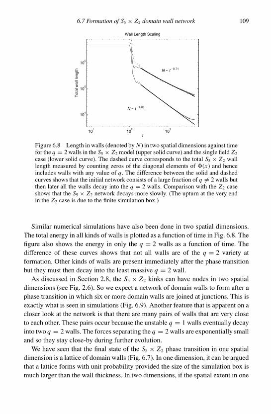
6.7 Formation of S5 × Z2 domain wall network 109
101
102
103
104
105
106
N ~ t −0.71
N ~ t −1.06
Tot
al w
all l
engt
h
t
Wall Length Scaling
Figure 6.8 Length in walls (denoted by N ) in two spatial dimensions against timefor the q = 2 walls in the S5 × Z2 model (upper solid curve) and the single field Z2case (lower solid curve). The dashed curve corresponds to the total S5 × Z2 walllength measured by counting zeros of the diagonal elements of (x) and henceincludes walls with any value of q . The difference between the solid and dashedcurves shows that the initial network consists of a large fraction of q = 2 walls butthen later all the walls decay into the q = 2 walls. Comparison with the Z2 caseshows that the S5 × Z2 network decays more slowly. (The upturn at the very endin the Z2 case is due to the finite simulation box.)
Similar numerical simulations have also been done in two spatial dimensions.The total energy in all kinds of walls is plotted as a function of time in Fig. 6.8. Thefigure also shows the energy in only the q = 2 walls as a function of time. Thedifference of these curves shows that not all walls are of the q = 2 variety atformation. Other kinds of walls are present immediately after the phase transitionbut they must then decay into the least massive q = 2 wall.
As discussed in Section 2.8, the S5 × Z2 kinks can have nodes in two spatialdimensions (see Fig. 2.6). So we expect a network of domain walls to form after aphase transition in which six or more domain walls are joined at junctions. This isexactly what is seen in simulations (Fig. 6.9). Another feature that is apparent on acloser look at the network is that there are many pairs of walls that are very closeto each other. These pairs occur because the unstable q = 1 walls eventually decayinto two q = 2 walls. The forces separating the q = 2 walls are exponentially smalland so they stay close-by during further evolution.
We have seen that the final state of the S5 × Z2 phase transition in one spatialdimension is a lattice of domain walls (Fig. 6.7). In one dimension, it can be arguedthat a lattice forms with unit probability provided the size of the simulation box ismuch larger than the wall thickness. In two dimensions, if the spatial extent in one

110 Formation of kinks
Figure 6.9 Network of S5 × Z2 walls in two spatial dimensions soon after thephase transition. The picture looks very similar to the network of (one-dimensional)walls connected to a network of (point-like) strings studied in [130].
direction is smaller than that in the other direction, so that the simulation box isrectangular with periodic boundary conditions, the evolution is very much like inone dimension and a lattice forms once again (see Fig. 6.10). Even on a square two-dimensional simulation box, a domain wall lattice is seen to form with a probability∼ 0.05 [7].
6.8 Biased phase transitions
The existence of domain walls relies only on the existence of discrete vacua. Thenit is possible to imagine situations where the degeneracy of the discrete vacuais slightly broken (see Fig. 6.11).4 Now the probability that the higher energyvacuum is selected during the phase transition in some region is less than 1/2and the probability that the lower energy vacuum is selected is larger than 1/2.This process can again be simulated on a square lattice by throwing down blacksquares with probability p < 1/2. If p is very small, there are only a few blacksquares and these are disconnected from each other. So the domain walls are small
4 Or perhaps the vacua are exactly degenerate but the likelihood of being in one particular vacuum is slightlylarger because of the way in which the system was prepared.

6.8 Biased phase transitions 111
0 50 100 150 200 250 300 350 400 450 5000
50
100
150t=
500
0 50 100 150 200 250 300 350 400 450 5000
50
100
150
t= 1
000
0 50 100 150 200 250 300 350 400 450 5000
50
100
150
t= 5
000
Figure 6.10 Three stages for the domain wall network evolution in a toroidal do-main, with dimensions Lx = 500 and L y = 150. The different shades correspondto the five possible charges of the domain walls (see Section 2.7). Note that in thebottom figure there is a pair of neighboring wall and antiwall of the same type (thewalls just before and after the 300 mark). These later annihilate, leading to a finalstable lattice consisting of ten walls.
V
f0
Figure 6.11 An asymmetric well in which the degeneracy of the vacua is slightlybroken.

112 Formation of kinks
and closed. At a critical value of p, call it pc, the black squares connect and thedistribution is dominated by one infinite cluster of black squares. Then the blacksquares are said to percolate. Therefore the domain wall formation problem reducesto the classic problem of “percolation theory” [143, 96, 36] where we are interestedin the critical probability and also the critical exponents that appear in variouscorrelation functions as the critical point is approached. On a triangular lattice intwo dimensions, the critical probability is known to be 0.5 and on a cubic lattice inthree dimensions it is 0.31. The problem may even be studied on a random latticeas discussed in [95].
The analysis for biased domain walls implies that even if the potential is slightlyasymmetric, infinite domain walls can form. For the SU (5) × Z2 potential describedin Eq. (2.5), the asymmetry is due to the cubic term with coupling constant, γ . Forsmall but non-zero values of γ , infinite domain walls form.
6.9 Open questions
1. What is the number density of domain walls formed in a second-order phase transition?The question may need to be sharpened since the density keeps changing with time.Also, while the number density is important in cosmology, condensed matter physicistsare mainly concerned with scaling laws (critical exponents) since these are expected tobe universal. So a sharper question would be in terms of a critical exponent related tothe number density (e.g. Eq. (6.60)).
2. Is there a condensed matter system which gives a domain wall lattice?3. Is there any role for domain wall lattices in (higher dimensional) cosmology?4. If a domain wall lattice can be generalized to strings and monopoles, do string and
monopole lattices form during a phase transition?

7
Dynamics of domain walls
In this chapter we discuss the dynamics of kinks and domain walls first in the zerothickness approximation, and then briefly in the full field theory. The zero thicknessapproximation can be expected to be valid in the case when all other length scales,such as the radii of curvature of a domain wall, are much larger than the wallthickness.1 We start by deriving the action for a kink in 1 + 1 dimensions as thisis the simplest case and contains the essential features of the higher dimensionalcases. Then we derive the action for a domain wall in 3 + 1 dimensions and someconsequences. In this chapter we ignore gravitational effects which can be quiteimportant in certain situations (see Chapter 8).
7.1 Kinks in 1 + 1 dimensions
In 1 + 1 dimensions, if we ignore the structure of the kink, then we expect the kinkto behave simply as a massive point particle. Its dynamics are then given by theusual action for a massive point particle
S1+1 = −M∫
dτ (7.1)
where M is the mass of the kink and dτ is the line element which may also bewritten as
dτ = dt
(gµν
dXµ
dt
dX ν
dt
)1/2
(7.2)
where gµν is the metric of the space-time background and Xµ(t) is the location ofthe kink at time t .
While the action in Eq. (7.1) seems reasonable on physical grounds, there shouldbe a systematic way to derive it starting from the original field theory action of which
1 This expectation is not completely correct since the wall velocity is also important [183, 73].
113
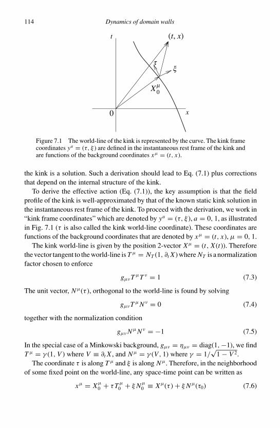
114 Dynamics of domain walls
t
xt
(t, x)
x0
X0m
Figure 7.1 The world-line of the kink is represented by the curve. The kink framecoordinates ya = (τ, ξ ) are defined in the instantaneous rest frame of the kink andare functions of the background coordinates xµ = (t, x).
the kink is a solution. Such a derivation should lead to Eq. (7.1) plus correctionsthat depend on the internal structure of the kink.
To derive the effective action (Eq. (7.1)), the key assumption is that the fieldprofile of the kink is well-approximated by that of the known static kink solution inthe instantaneous rest frame of the kink. To proceed with the derivation, we work in“kink frame coordinates” which are denoted by ya = (τ, ξ ), a = 0, 1, as illustratedin Fig. 7.1 (τ is also called the kink world-line coordinate). These coordinates arefunctions of the background coordinates that are denoted by xµ = (t, x), µ = 0, 1.
The kink world-line is given by the position 2-vector Xµ = (t, X (t)). Thereforethe vector tangent to the world-line is T µ = NT (1, ∂t X ) where NT is a normalizationfactor chosen to enforce
gµνT µT ν = 1 (7.3)
The unit vector, Nµ(τ ), orthogonal to the world-line is found by solving
gµνT µN ν = 0 (7.4)
together with the normalization condition
gµν NµN ν = −1 (7.5)
In the special case of a Minkowski background, gµν = ηµν = diag(1, −1), we findT µ = γ (1, V ) where V ≡ ∂t X , and Nµ = γ (V, 1) where γ = 1/
√1 − V 2.
The coordinate τ is along T µ and ξ is along Nµ. Therefore, in the neighborhoodof some fixed point on the world-line, any space-time point can be written as
xµ = Xµ
0 + τT µ
0 + ξ Nµ
0 ≡ Xµ(τ ) + ξ Nµ(τ0) (7.6)

7.1 Kinks in 1 + 1 dimensions 115
where the subscript 0 refers to the fixed point on the world-line. Since the energydensity in the fields vanishes far from the kink, only the neighborhood of the world-line is relevant for deriving the effective action. Hence ξ is small and to lowest orderwe can replace τ0 in the last term by τ to get
xµ = Xµ(τ ) + ξ Nµ(τ ) (7.7)
With the coordinate transformation in Eq. (7.7), the world-line metric can bewritten in the ya coordinate system
hab = gµν∂axµ∂bxν (7.8)
Therefore
h00 = gµν(∂τ Xµ + ξ∂τ Nµ)(∂τ X ν + ξ∂τ N ν)
= gµν∂τ Xµ∂τ X ν + O(ξ )
h01 = gµν(∂τ Xµ + ξ∂τ Nµ)N ν = O(ξ )
h11 = gµν NµN ν = −1
where we have used the orthogonality of ∂τ Xµ ∝ T µ and Nµ, and the normalizationof Nµ. So the determinant of hab is
h = −gµν(Xµ)∂τ Xµ∂τ X ν + O(ξ ) (7.9)
where we have also expanded the background metric around the kink location.Next we write,
φ(xµ) = φ0(ya) + ψ(ya) (7.10)
where φ0 is the static kink profile function in the kink frame coordinates. Forexample, in the case of the Z2 kink, φ0 = η tanh(
√λ/2 ηξ ) (see Eq. (1.9)). The
field ψ is the departure of the true field configuration from the static kink profileφ0. The assumption is that the contribution of ψ to the action is small and hence ψ
can be used as a parameter for a perturbative expansion.Now the field theory action is
S =∫
d2x√−gL[φ, φ; gµν] (7.11)
in terms of the Lagrangian density L and g = Det(gµν). The metric is taken to bea fixed background and the gravitational effects of the wall are ignored. The fullproblem of gravitating domain walls is significantly more complicated at a technicallevel [21].
Now we write this action in the kink frame coordinates to get
S = S0 + O(ξ, ψ) (7.12)
116 Dynamics of domain walls
with
S0 =∫
dτdξ√
|h| L[φ0(ξ ), φ0(ξ ); hab]
=∫
dτ√
|h|∫
dξ L[φ0(ξ ), 0; hab]
= −M∫
dτ√
|h| (7.13)
where M is the mass of the kink. The last equality follows since the solution isstatic and hence the Lagrangian density equals the energy density up to a sign.The integration of the Lagrangian density then gives the −M factor. The effectiveaction is therefore the action for a point particle, simply given by the length of theworld-line. This result can easily be extended to walls (and strings) propagating inhigher dimensions, and the leading term in the effective action is proportional to theworld volume. Such geometric effective actions are often referred to as “Nambu-Goto actions.” Even if the self-gravity of the domain wall is taken into account, thedominant contribution to the effective action is still the Nambu-Goto action [21].
The next-to-leading order terms in the effective action, denoted by O(ξ, ψ) inEq. (7.12), have been discussed for domain walls in [138, 21, 73, 28], building onthe earlier analysis for strings [57, 105, 72]. The first-order corrections in both ψ
and ξ vanish because the field φ0 is a solution of the equation of motion and hencethe action is an extremum at φ0. The lowest non-trivial corrections come at secondorder in ξ and ψ . An alternative approach to studying domain wall dynamics hasbeen developed in [9].
Finally we remark that the parameter τ can be chosen arbitrarily. Any otherworld-line coordinate, τ ′(τ ), leaves the effective action invariant. This fact is called“reparametrization invariance” of the action.
7.2 Walls in 3 + 1 dimensions
The location of a domain wall, Xµ(τ, ζ, χ ), is described by three world-volumecoordinates ya = (τ, ζ, χ ). Any point, xµ, can now be written in terms of the “wallframe coordinates” (see Eq. (7.6) and Fig. 7.2)
xµ = Xµ(τ, ζ, χ ) + ξ Nµ(τ, ζ, χ ) (7.14)
where Nµ is the normal to the wall.The derivation of the Nambu-Goto action proceeds exactly as in the kink case
of the last section and we get
S0 = −σ
∫d3ρ√
|h| (7.15)
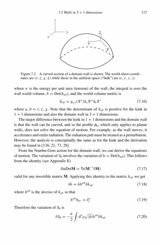
7.2 Walls in 3 + 1 dimensions 117
z
x
zc
xy
Figure 7.2 A curved section of a domain wall is shown. The world-sheet coordi-nates are (τ, ζ, χ, ξ ) while those in the ambient space (“bulk”) are (t, x, y, z).
where σ is the energy per unit area (tension) of the wall, the integral is over thewall world volume, h = Det(hab), and the world-volume metric is
hab = gµν(Xρ)∂a Xµ∂b X ν (7.16)
where a, b = τ, ζ, χ . Note that the determinant of hab is positive for the kink in1 + 1 dimensions and also the domain wall in 3 + 1 dimensions.
The major difference between the kink in 1 + 1 dimensions and the domain wallis that the wall can be curved, and so the profile φ0, which only applies to planarwalls, does not solve the equation of motion. For example, as the wall moves, itaccelerates and emits radiation. The radiation part must be treated as a perturbation.However, the analysis is conceptually the same as for the kink and the derivationmay be found in [138, 21, 73, 28].
From the Nambu-Goto action for the domain wall, we can derive the equationsof motion. The variation of S0 involves the variation of h = Det(hαβ). This followsfrom the identity (see Appendix E)
δlnDetM = Tr(M−1δM) (7.17)
valid for any invertible matrix M. Applying this identity to the matrix hab we get
δh = hhabδhab (7.18)
where hab is the inverse of hab so that
habhbc = δac (7.19)
Therefore the variation of S0 is
δS0 = −σ
2
∫d3ρ√
|h|habδhab (7.20)
118 Dynamics of domain walls
We obtain the wall equation of motion by requiring δS0 = 0 together with thedefinition of hab in Eq. (7.16)
1√|h|∂a(√
|h|hab∂b Xσ ) = σµνhab∂a Xµ∂b X ν (7.21)
where the Christoffel symbol is defined by the background metric gµν
σµν = gσρ
2(∂νgρµ + ∂µgρν − ∂ρgµν) (7.22)
In the special case of a Minkowski background metric, the Christoffel symbolvanishes and
1√|h|∂a(√
|h|hab∂b Xσ ) = 0 (7.23)
Using Eq. (7.17), the determinant h can be eliminated and the equation of motioncan be written as
∂a(hab∂b Xσ ) + 1
2hcd∂ahcd hab∂b Xσ = 0 (7.24)
The equation of motion for a wall is highly non-linear because hab itself isdefined as a quadratic in derivatives of Xµ. One way to simplify the equations is tochoose convenient coordinates. This is possible because the equations of motionof the wall are reparametrization invariant, i.e. we are free to choose any world-volume coordinates (τ, ζ, χ ). A similar situation occurs for strings that have a 1 + 1dimensional world sheet. There, by a choice of coordinates, the equation of motioncan be converted to a simple wave equation in 1 + 1 dimensions together with somequadratic constraints that can be solved quite generally. In the case of the domainwall, however, no such convenient choice of coordinates is known and the equationshave not been solved in general. Only a few special solutions are known. Of these,static solutions subject to suitable boundary conditions have minimal surface area,and these have been extensively studied in the mathematics literature e.g. [115].
In a realistic setting, the dynamics of the walls are affected by inter-kink forces,by the interaction of any surrounding particles, the gravitational field of the wall, andthe evolution of the background space-time. In addition, there are collisions betweendifferent walls, leading to intercommuting (Section 3.8), and annihilation of wallsand antiwalls. If there are zero modes on the walls as described in Chapter 5, theycould also carry charges and currents and this would introduce other interactions.
7.3 Some solutions
In 1 + 1 dimensions the kink moves like a point particle of mass M . The dynamicsare richer in 3 + 1 dimensions where a closed domain wall can oscillate and movein complicated ways. The Nambu-Goto action is valid when the radii of curvature of
7.3 Some solutions 119
the wall and the separation of different sections of wall are both large compared tothe thickness of the wall. In addition, the velocity of the wall (in the center of massframe) should be small. (See Section 7.3.3 for the criterion in the case of collapsingspherical domain walls.) When these conditions are not met, the only way to proceedis to consider the dynamics using the underlying field theory. In this section, weignore field theory effects and describe some solutions to the Nambu-Goto action.
7.3.1 Planar solutions: traveling waves
A planar domain wall in the z = 0 plane is given by
Xµ(τ, ζ, χ ) = (τ, ζ, χ, 0) (7.25)
Next consider a planar domain wall with some ripples
Xµ(τ, ζ, χ ) = (τ, ζ, χ, z(τ, ζ, χ )) (7.26)
The function z describes the ripples and we would like solutions for z.For the wall in Eq. (7.26), the world-volume metric is
hab = ηab − ∂az∂bz (7.27)
where
ηab = diag(1, −1, −1) (7.28)
Inverting hab is not simple, but inverting ηab is. So consider the “trial” inversemetric
hbc = ηbc + ηbd∂d z ηce∂ez (7.29)
Then by evaluating habhbc, it can be seen that hbc is the correct inverse metricprovided
ηab∂az∂bz = 0 (7.30)
Now we can use Eq. (7.24) and the constraint (7.30) to get the equation of motionfor the function z(τ, ζ, χ )
∂a∂az = 0 (7.31)
Hence any function that satisfies Eqs. (7.31) and (7.30) extremizes the Nambu-Gotoaction for a domain wall.
Solutions of Eqs. (7.31) and (7.30) have been discussed in [58]. The constraintcondition implies that the solution must necessarily be time-dependent. A class ofsolutions is obtained by noting, for example, that z = f (τ − ζ ) solves the equationof motion and also the constraint for any choice of function f . This correspondsto a pulse of arbitrary shape on a planar domain wall that propagates in the +x
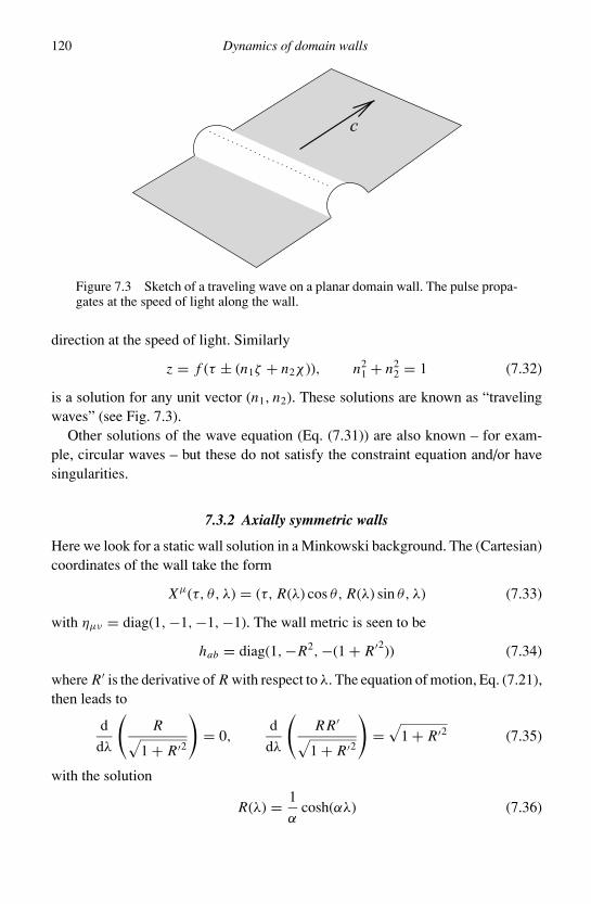
120 Dynamics of domain walls
c
Figure 7.3 Sketch of a traveling wave on a planar domain wall. The pulse propa-gates at the speed of light along the wall.
direction at the speed of light. Similarly
z = f (τ ± (n1ζ + n2χ )), n21 + n2
2 = 1 (7.32)
is a solution for any unit vector (n1, n2). These solutions are known as “travelingwaves” (see Fig. 7.3).
Other solutions of the wave equation (Eq. (7.31)) are also known – for exam-ple, circular waves – but these do not satisfy the constraint equation and/or havesingularities.
7.3.2 Axially symmetric walls
Here we look for a static wall solution in a Minkowski background. The (Cartesian)coordinates of the wall take the form
Xµ(τ, θ, λ) = (τ, R(λ) cos θ, R(λ) sin θ, λ) (7.33)
with ηµν = diag(1, −1, −1, −1). The wall metric is seen to be
hab = diag(1, −R2, −(1 + R′2)) (7.34)
where R′ is the derivative of R with respect to λ. The equation of motion, Eq. (7.21),then leads to
d
dλ
(R√
1 + R′2
)= 0,
d
dλ
(R R′√
1 + R′2
)=√
1 + R′2 (7.35)
with the solution
R(λ) = 1
αcosh(αλ) (7.36)

7.3 Some solutions 121
da −1
D
Figure 7.4 Sketch of a catenoid solution.
where α is a parameter, τ = t , λ = z and θ is the angle in cylindrical coordinates.Equation (7.36) describes a one-parameter family of static, axially symmetric, do-main wall solutions (see Fig. 7.4).
The solution in Eq. (7.36) is a catenoid that is seen in soap films which, likedomain walls, also minimize their surface area [23]. Experiments with soap filmsare done with two parallel circular rings, each of diameter D, placed a certaindistance, d , apart. Then the soap film forms a catenoid for d/D < 0.66 [117].Actually there are two catenoid solutions for d/D < 0.66 since the relation αD =cosh(αd/2) has two solutions for α for fixed values of D and d in this regime. Athird solution, which consists of two disconnected disks circumscribed by each ofthe circular rings also exists. For larger values of the separation-to-diameter ratio,d/D, the two-disk solution has less surface area than the catenoid solutions, andthe catenoid can pinch off and minimize its area by transforming to the two disks.It seems reasonable to assume that the soap film analysis also applies to the domainwall.
The catenoid is a static solution of the Nambu-Goto equations of motion. Itcould happen that the catenoid is not a solution of the field equations. A simpleexample of a solution to the Nambu-Goto equations that does not solve the fieldequations can be constructed quite easily. Two parallel planar walls (a wall andan antiwall) form a solution to the Nambu-Goto equations but, since these wallshave an exponentially small attractive force, they do not form a solution to thefield equations. However, by fixing the boundary conditions (as in the soap filmcase by the rings), the catenoid solution for domain walls has been constructednumerically by solving the equations of motion for the scalar field in the Z2 model(Sutcliffe, P., 2005, private communication). The stability of the catenoid solutionto the Nambu-Goto equations is an open question (Section 7.7).

122 Dynamics of domain walls
Quite complicated static domain wall solutions have also been studied in thecontext of quasicrystals [137] and microemulsions [70].
In addition to static solutions, we could seek time-dependent solutions with axialsymmetry. The simplest such case would be a cylindrical domain wall whose radiusis a function of time. The radius would contract, pass through zero, and then growagain. A similar solution is obtained for spherical walls which we discuss moreexplicitly in the next section.
To obtain the cylindrical solution, we note that energy is conserved during col-lapse. The energy per unit length of a cylindrical wall is
= σ2π R√1 − R2
= constant (7.37)
where σ is the energy per unit area of the wall, R is the radius of the cylinder attime t , and an overdot denotes differentiation with respect to t . The square rootfactor in the denominator takes care of the Lorentz boost.
The conservation of energy (i.e. constancy of ), immediately leads to thesolution
R(t) = R0 cos
(t
R0
)(7.38)
where R0 = /σ2π is the radius when the wall is at rest.
7.3.3 Spherical walls
Our final example of domain wall solutions is with a spherical ansatz
Xµ(τ, θ, φ) = (τ, R(τ )r) (7.39)
where
τ = t, r = (sin θ cos φ, sin θ sin φ, cos θ ) (7.40)
and θ, φ are spherical angular coordinates. The space-time metric is ηµν =diag(1, −1, −1, −1).
We now find
hab = diag(1 − R2, −R2, −R2 sin2 θ) (7.41)
where overdots denote derivatives with respect to τ . After some algebra, fromEq. (7.21) we obtain the equation of motion
R = − 2
R(1 − R2) (7.42)

7.3 Some solutions 123
R
t
Figure 7.5 Radius of a collapsing spherical domain wall against time in the thinwall approximation. The coordinates in the plot are in units of the maximum radiusof the wall.
For R = 0, R2 = 0, 1 this can also be written as
d
dτ
(R2√
1 − R2
)= 0 (7.43)
which implies
4πσR2√
1 − R2= M (7.44)
where M is a constant of motion, to be identified with the mass of the sphericaldomain wall (σ is the mass per unit area of the wall).
The solution can be written in terms of the elliptic integral of the first kind∫ x
x∗
dx√1 − x4
= ±τ − τ0
R0(7.45)
where
R20 ≡ M
4πσ, x ≡ R
R0(7.46)
R0 has the interpretation of being the radius when the wall is at rest and x∗ is thevalue of x at some initial time τ0. The sign in Eq. (7.45) is chosen according towhether one is interested in the expanding or contracting solution. The radius of acollapsing spherical domain wall is plotted in Fig. 7.5.
The behavior of perturbations on the spherical domain wall has been studied in[182]. The result is that at late times the ratio of the perturbation amplitude dividedby the radius of the spherical wall, grows as 1/R as the wall collapses.
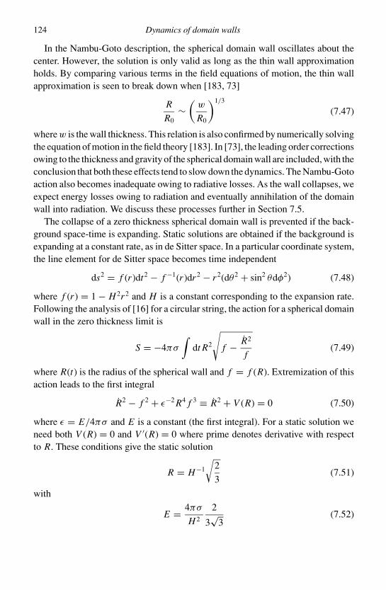
124 Dynamics of domain walls
In the Nambu-Goto description, the spherical domain wall oscillates about thecenter. However, the solution is only valid as long as the thin wall approximationholds. By comparing various terms in the field equations of motion, the thin wallapproximation is seen to break down when [183, 73]
R
R0∼(
w
R0
)1/3
(7.47)
where w is the wall thickness. This relation is also confirmed by numerically solvingthe equation of motion in the field theory [183]. In [73], the leading order correctionsowing to the thickness and gravity of the spherical domain wall are included, with theconclusion that both these effects tend to slow down the dynamics. The Nambu-Gotoaction also becomes inadequate owing to radiative losses. As the wall collapses, weexpect energy losses owing to radiation and eventually annihilation of the domainwall into radiation. We discuss these processes further in Section 7.5.
The collapse of a zero thickness spherical domain wall is prevented if the back-ground space-time is expanding. Static solutions are obtained if the background isexpanding at a constant rate, as in de Sitter space. In a particular coordinate system,the line element for de Sitter space becomes time independent
ds2 = f (r )dt2 − f −1(r )dr2 − r2(dθ2 + sin2 θdφ2) (7.48)
where f (r ) = 1 − H 2r2 and H is a constant corresponding to the expansion rate.Following the analysis of [16] for a circular string, the action for a spherical domainwall in the zero thickness limit is
S = −4πσ
∫dt R2
√f − R2
f(7.49)
where R(t) is the radius of the spherical wall and f = f (R). Extremization of thisaction leads to the first integral
R2 − f 2 + ε−2 R4 f 3 ≡ R2 + V (R) = 0 (7.50)
where ε = E/4πσ and E is a constant (the first integral). For a static solution weneed both V (R) = 0 and V ′(R) = 0 where prime denotes derivative with respectto R. These conditions give the static solution
R = H−1
√2
3(7.51)
with
E = 4πσ
H 2
2
3√
3(7.52)
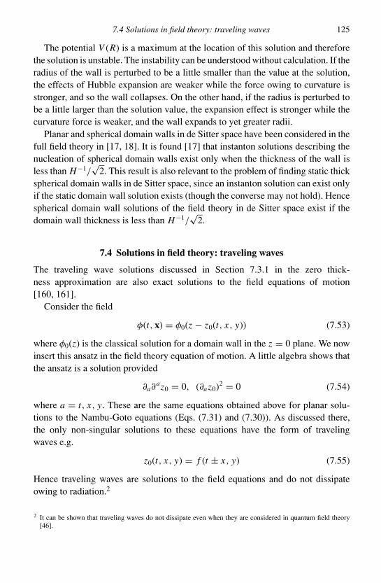
7.4 Solutions in field theory: traveling waves 125
The potential V (R) is a maximum at the location of this solution and thereforethe solution is unstable. The instability can be understood without calculation. If theradius of the wall is perturbed to be a little smaller than the value at the solution,the effects of Hubble expansion are weaker while the force owing to curvature isstronger, and so the wall collapses. On the other hand, if the radius is perturbed tobe a little larger than the solution value, the expansion effect is stronger while thecurvature force is weaker, and the wall expands to yet greater radii.
Planar and spherical domain walls in de Sitter space have been considered in thefull field theory in [17, 18]. It is found [17] that instanton solutions describing thenucleation of spherical domain walls exist only when the thickness of the wall isless than H−1/
√2. This result is also relevant to the problem of finding static thick
spherical domain walls in de Sitter space, since an instanton solution can exist onlyif the static domain wall solution exists (though the converse may not hold). Hencespherical domain wall solutions of the field theory in de Sitter space exist if thedomain wall thickness is less than H−1/
√2.
7.4 Solutions in field theory: traveling waves
The traveling wave solutions discussed in Section 7.3.1 in the zero thick-ness approximation are also exact solutions to the field equations of motion[160, 161].
Consider the field
φ(t, x) = φ0(z − z0(t, x, y)) (7.53)
where φ0(z) is the classical solution for a domain wall in the z = 0 plane. We nowinsert this ansatz in the field theory equation of motion. A little algebra shows thatthe ansatz is a solution provided
∂a∂az0 = 0, (∂az0)2 = 0 (7.54)
where a = t, x, y. These are the same equations obtained above for planar solu-tions to the Nambu-Goto equations (Eqs. (7.31) and (7.30)). As discussed there,the only non-singular solutions to these equations have the form of travelingwaves e.g.
z0(t, x, y) = f (t ± x, y) (7.55)
Hence traveling waves are solutions to the field equations and do not dissipateowing to radiation.2
2 It can be shown that traveling waves do not dissipate even when they are considered in quantum field theory[46].
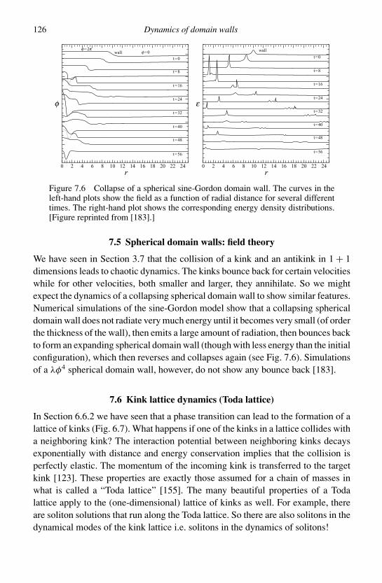
126 Dynamics of domain walls
0 2 4 6 8 10 12 14 16 18 20 22 24
t=56
t=48
t=40
t=32
t=24
t=16
t=8
t=0 t=0
t=8
t=16
t=24
t=32
t=40
t=48
t=56
f=0f=2p
wall wall
0
e
rr
f
2 4 6 8 10 12 14 16 18 20 22 24
Figure 7.6 Collapse of a spherical sine-Gordon domain wall. The curves in theleft-hand plots show the field as a function of radial distance for several differenttimes. The right-hand plot shows the corresponding energy density distributions.[Figure reprinted from [183].]
7.5 Spherical domain walls: field theory
We have seen in Section 3.7 that the collision of a kink and an antikink in 1 + 1dimensions leads to chaotic dynamics. The kinks bounce back for certain velocitieswhile for other velocities, both smaller and larger, they annihilate. So we mightexpect the dynamics of a collapsing spherical domain wall to show similar features.Numerical simulations of the sine-Gordon model show that a collapsing sphericaldomain wall does not radiate very much energy until it becomes very small (of orderthe thickness of the wall), then emits a large amount of radiation, then bounces backto form an expanding spherical domain wall (though with less energy than the initialconfiguration), which then reverses and collapses again (see Fig. 7.6). Simulationsof a λφ4 spherical domain wall, however, do not show any bounce back [183].
7.6 Kink lattice dynamics (Toda lattice)
In Section 6.6.2 we have seen that a phase transition can lead to the formation of alattice of kinks (Fig. 6.7). What happens if one of the kinks in a lattice collides witha neighboring kink? The interaction potential between neighboring kinks decaysexponentially with distance and energy conservation implies that the collision isperfectly elastic. The momentum of the incoming kink is transferred to the targetkink [123]. These properties are exactly those assumed for a chain of masses inwhat is called a “Toda lattice” [155]. The many beautiful properties of a Todalattice apply to the (one-dimensional) lattice of kinks as well. For example, thereare soliton solutions that run along the Toda lattice. So there are also solitons in thedynamical modes of the kink lattice i.e. solitons in the dynamics of solitons!

7.7 Open questions 127
7.7 Open questions
1. Are there closed domain walls in three dimensions that do not self-intersect as theyoscillate? What happens in higher dimensions?
2. Can one show analytically that walls must intercommute on intersection?3. When traveling waves on domain walls collide, they dissipate some of their energy. Find
the energy radiated. Find the energy that goes into excitations of the bound state in thecase of the Z2 wall.
4. Analyze the catenoid domain wall solution and its stability.

8
Gravity and cosmology of domain walls
Domain walls resulting from a symmetry breaking in the early universe could havenovel and dramatic gravitational and cosmological consequences.
We first derive the gravitational effects of a planar domain wall, describing thedifferent ways to view the system. Then we discuss spherical walls as an exampleof curved domain walls. To discuss the cosmological consequences, it is necessaryto have a picture of domain wall formation in the cosmological context. Withthe background of Chapter 6 we discuss the formation of the wall network incosmology, then the evolution and cosmological implications. We end by reviewingthe cosmological constraints on domain walls and the few possible ways aroundthe constraints.
8.1 Energy-momentum of domain walls
The energy-momentum tensor for a scalar field with potential V (φ) is given inEq. (1.39)
Tµν = ∂µφ∂νφ − gµν
1
2(∂αφ)2 − V (φ)
(8.1)
In the thin-wall limit, varying the Nambu-Goto action (Eq. (7.15)) gives the energy-momentum tensor
T µν
∣∣∣∣NG
= σ√−g
∫d3ρ√
|h| hab∂a Xµ∂b X ν δ(4)(xµ − Xµ) (8.2)
where Xµ is the location of the wall. For a planar wall located at x = 0 in flatspace-time, this gives
T µν
∣∣∣∣NG,plane
= σ (1, 0, −1, −1)δ(x) (8.3)
128
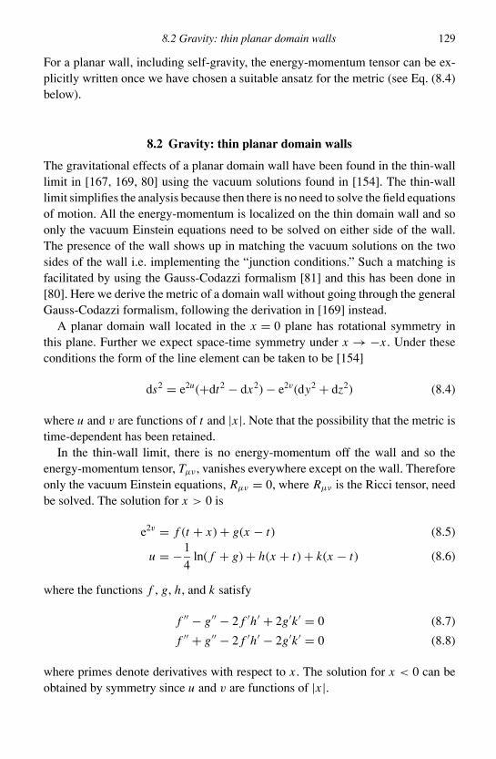
8.2 Gravity: thin planar domain walls 129
For a planar wall, including self-gravity, the energy-momentum tensor can be ex-plicitly written once we have chosen a suitable ansatz for the metric (see Eq. (8.4)below).
8.2 Gravity: thin planar domain walls
The gravitational effects of a planar domain wall have been found in the thin-walllimit in [167, 169, 80] using the vacuum solutions found in [154]. The thin-walllimit simplifies the analysis because then there is no need to solve the field equationsof motion. All the energy-momentum is localized on the thin domain wall and soonly the vacuum Einstein equations need to be solved on either side of the wall.The presence of the wall shows up in matching the vacuum solutions on the twosides of the wall i.e. implementing the “junction conditions.” Such a matching isfacilitated by using the Gauss-Codazzi formalism [81] and this has been done in[80]. Here we derive the metric of a domain wall without going through the generalGauss-Codazzi formalism, following the derivation in [169] instead.
A planar domain wall located in the x = 0 plane has rotational symmetry inthis plane. Further we expect space-time symmetry under x → −x . Under theseconditions the form of the line element can be taken to be [154]
ds2 = e2u(+dt2 − dx2) − e2v(dy2 + dz2) (8.4)
where u and v are functions of t and |x |. Note that the possibility that the metric istime-dependent has been retained.
In the thin-wall limit, there is no energy-momentum off the wall and so theenergy-momentum tensor, Tµν , vanishes everywhere except on the wall. Thereforeonly the vacuum Einstein equations, Rµν = 0, where Rµν is the Ricci tensor, needbe solved. The solution for x > 0 is
e2v = f (t + x) + g(x − t) (8.5)
u = −1
4ln( f + g) + h(x + t) + k(x − t) (8.6)
where the functions f , g, h, and k satisfy
f ′′ − g′′ − 2 f ′h′ + 2g′k ′ = 0 (8.7)
f ′′ + g′′ − 2 f ′h′ − 2g′k ′ = 0 (8.8)
where primes denote derivatives with respect to x . The solution for x < 0 can beobtained by symmetry since u and v are functions of |x |.

130 Gravity and cosmology of domain walls
Next we solve the Einstein equations, Tµν = Gµν/8πG, where Gµν is theEinstein tensor calculated for the metric in Eq. (8.4). This leads to
T 00 = 1
4πGv′
0e−2u0δ(x)
T 11 = 0
T 22 = T 3
3 = − 1
8πG(u′
0 + v′0)e−2u0δ(x) (8.9)
where u0 = u(t, x = 0+), v0 = v(t, x = 0+).In general, u0, u′
0, and v′0 are time-dependent, and so these expressions for T µ
ν arealso time-dependent. However, the energy-momentum tensor for the wall shouldbe time-independent. This gives us the constraint that the functions f , g, h, and kmust be chosen so that u0, u′
0, and v′0 are time-independent. Then the only possible
choice for the functions (for x > 0) that also satisfy Eq. (8.8) is
f = 0, g = eK (t−x)
h = − K
4(t + x), k = K
2(t − x) (8.10)
where
K = 4πGσ (8.11)
The corresponding functions for x < 0 are
f = eK (t+x), g = 0
h = K
2(t + x), k = − K
4(t − x) (8.12)
Then the domain wall line element is
ds2 = e−K |x |[dt2 − dx2 − eK t (dy2 + dz2)] (8.13)
which can also be put in the commonly encountered form
ds2 = (1 − κ|X |)2dt2 − dX2 − (1 − κ|X |)2e2κt (dy2 + dz2) (8.14)
where κ = 2πGσ via the coordinate transformation
|X | = 1
κ(1 − e−κ|x |) (8.15)
8.3 Gravitational properties of the thin planar wall
On spatial slices of constant X (X = X0) the metric of Eq. (8.14) takes the form
ds23 = dt2 − e2κ t (dy2 + dz2) (8.16)
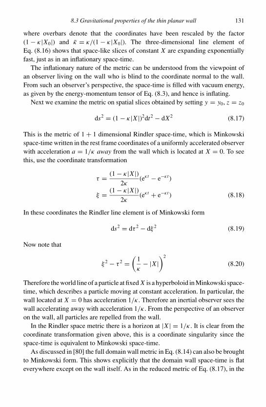
8.3 Gravitational properties of the thin planar wall 131
where overbars denote that the coordinates have been rescaled by the factor(1 − κ|X0|) and κ = κ/(1 − κ|X0|). The three-dimensional line element ofEq. (8.16) shows that space-like slices of constant X are expanding exponentiallyfast, just as in an inflationary space-time.
The inflationary nature of the metric can be understood from the viewpoint ofan observer living on the wall who is blind to the coordinate normal to the wall.From such an observer’s perspective, the space-time is filled with vacuum energy,as given by the energy-momentum tensor of Eq. (8.3), and hence is inflating.
Next we examine the metric on spatial slices obtained by setting y = y0, z = z0
ds2 = (1 − κ|X |)2dt2 − dX2 (8.17)
This is the metric of 1 + 1 dimensional Rindler space-time, which is Minkowskispace-time written in the rest frame coordinates of a uniformly accelerated observerwith acceleration a = 1/κ away from the wall which is located at X = 0. To seethis, use the coordinate transformation
τ = (1 − κ|X |)2κ
(eκt − e−κt )
ξ = (1 − κ|X |)2κ
(eκt + e−κt ) (8.18)
In these coordinates the Rindler line element is of Minkowski form
ds2 = dτ 2 − dξ 2 (8.19)
Now note that
ξ 2 − τ 2 =(
1
κ− |X |
)2
(8.20)
Therefore the world line of a particle at fixed X is a hyperboloid in Minkowski space-time, which describes a particle moving at constant acceleration. In particular, thewall located at X = 0 has acceleration 1/κ . Therefore an inertial observer sees thewall accelerating away with acceleration 1/κ . From the perspective of an observeron the wall, all particles are repelled from the wall.
In the Rindler space metric there is a horizon at |X | = 1/κ . It is clear from thecoordinate transformation given above, this is a coordinate singularity since thespace-time is equivalent to Minkowski space-time.
As discussed in [80] the full domain wall metric in Eq. (8.14) can also be broughtto Minkowski form. This shows explicitly that the domain wall space-time is flateverywhere except on the wall itself. As in the reduced metric of Eq. (8.17), in the
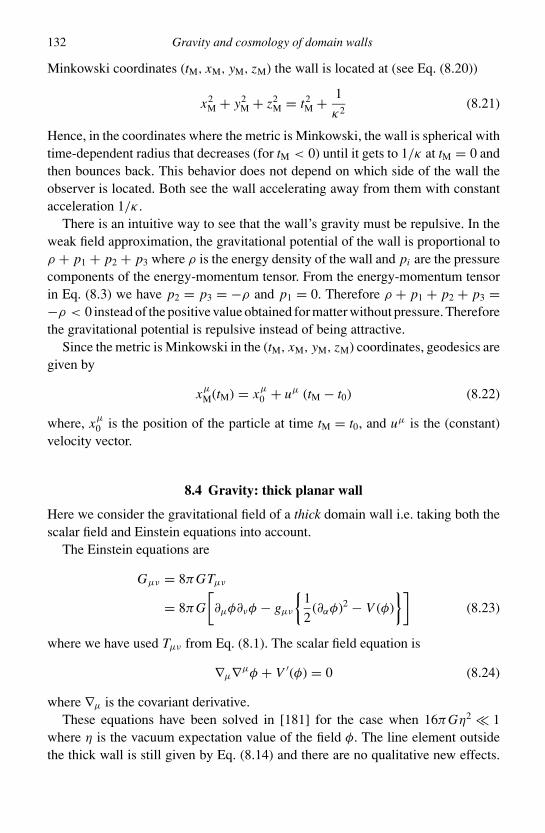
132 Gravity and cosmology of domain walls
Minkowski coordinates (tM, xM, yM, zM) the wall is located at (see Eq. (8.20))
x2M + y2
M + z2M = t2
M + 1
κ2(8.21)
Hence, in the coordinates where the metric is Minkowski, the wall is spherical withtime-dependent radius that decreases (for tM < 0) until it gets to 1/κ at tM = 0 andthen bounces back. This behavior does not depend on which side of the wall theobserver is located. Both see the wall accelerating away from them with constantacceleration 1/κ .
There is an intuitive way to see that the wall’s gravity must be repulsive. In theweak field approximation, the gravitational potential of the wall is proportional toρ + p1 + p2 + p3 where ρ is the energy density of the wall and pi are the pressurecomponents of the energy-momentum tensor. From the energy-momentum tensorin Eq. (8.3) we have p2 = p3 = −ρ and p1 = 0. Therefore ρ + p1 + p2 + p3 =−ρ < 0 instead of the positive value obtained for matter without pressure. Thereforethe gravitational potential is repulsive instead of being attractive.
Since the metric is Minkowski in the (tM, xM, yM, zM) coordinates, geodesics aregiven by
xµ
M(tM) = xµ
0 + uµ (tM − t0) (8.22)
where, xµ
0 is the position of the particle at time tM = t0, and uµ is the (constant)velocity vector.
8.4 Gravity: thick planar wall
Here we consider the gravitational field of a thick domain wall i.e. taking both thescalar field and Einstein equations into account.
The Einstein equations are
Gµν = 8πGTµν
= 8πG
[∂µφ∂νφ − gµν
1
2(∂αφ)2 − V (φ)
](8.23)
where we have used Tµν from Eq. (8.1). The scalar field equation is
∇µ∇µφ + V ′(φ) = 0 (8.24)
where ∇µ is the covariant derivative.These equations have been solved in [181] for the case when 16πGη2 1
where η is the vacuum expectation value of the field φ. The line element outsidethe thick wall is still given by Eq. (8.14) and there are no qualitative new effects.
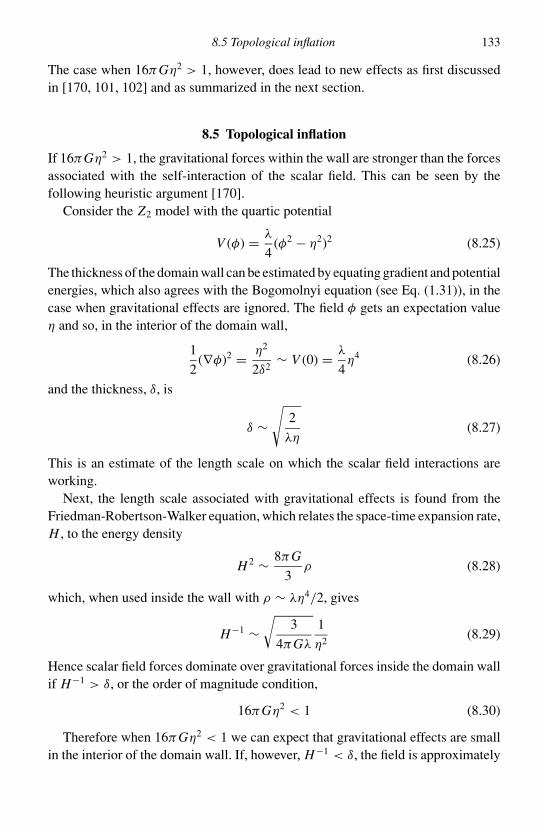
8.5 Topological inflation 133
The case when 16πGη2 > 1, however, does lead to new effects as first discussedin [170, 101, 102] and as summarized in the next section.
8.5 Topological inflation
If 16πGη2 > 1, the gravitational forces within the wall are stronger than the forcesassociated with the self-interaction of the scalar field. This can be seen by thefollowing heuristic argument [170].
Consider the Z2 model with the quartic potential
V (φ) = λ
4(φ2 − η2)2 (8.25)
The thickness of the domain wall can be estimated by equating gradient and potentialenergies, which also agrees with the Bogomolnyi equation (see Eq. (1.31)), in thecase when gravitational effects are ignored. The field φ gets an expectation valueη and so, in the interior of the domain wall,
1
2(∇φ)2 = η2
2δ2∼ V (0) = λ
4η4 (8.26)
and the thickness, δ, is
δ ∼√
2
λη(8.27)
This is an estimate of the length scale on which the scalar field interactions areworking.
Next, the length scale associated with gravitational effects is found from theFriedman-Robertson-Walker equation, which relates the space-time expansion rate,H , to the energy density
H 2 ∼ 8πG
3ρ (8.28)
which, when used inside the wall with ρ ∼ λη4/2, gives
H−1 ∼√
3
4πGλ
1
η2(8.29)
Hence scalar field forces dominate over gravitational forces inside the domain wallif H−1 > δ, or the order of magnitude condition,
16πGη2 < 1 (8.30)
Therefore when 16πGη2 < 1 we can expect that gravitational effects are smallin the interior of the domain wall. If, however, H−1 < δ, the field is approximately

134 Gravity and cosmology of domain walls
smooth over a region where gravitational effects are strong. The field inside thedomain wall has potential energy ∼ λη4 and this is what drives the gravitationaleffects. Therefore, we expect that the space-time inside the domain wall inflatesin the direction normal to the wall, in addition to the inflation parallel to the wallthat we have already seen in the thin-wall case (Eq. (8.14)). Furthermore, the fieldinside the wall is stuck on top of the potential owing to the topology that led tothe existence of the wall. So the inflation goes on forever for topological reasons.Hence this inflation is called “topological inflation.”
This picture has been confirmed by numerical solution of the coupled scalarfield and Einstein equations in [131, 31, 94] with the conclusion that topologicalinflation inside the Z2 domain wall occurs for η > 0.33mP where mP is the Planckmass defined by G = 1/m2
P.Domain walls that are undergoing topological inflation cannot however form in
the usual way during a cosmological phase transition as we discuss in Section 8.9below.
8.6 Spherical domain wall
The metric of a thin spherical domain wall has been discussed in the thin-wall limitin [80]. Inside the wall the metric is flat using Birkhoff’s theorem (e.g. see [177])
ds2 = dT 2 − dr2 − r2(dθ2 + sin2 θdφ2), r < R(t) (8.31)
where R(t) is the radius of the spherical wall and
T = (1 + R2)1/2 (8.32)
with overdots denoting derivatives with respect to the proper time of an observermoving with the domain wall. The proper time is related to the time coordinate tvia the relation (
1 − 2G M
R
)t =
(1 − 2G M
R+ R2
)1/2
(8.33)
Outside the sphere, the metric is Schwarzschild with mass parameter M
ds2 =(
1 − 2G M
r
)dt2 −
(1 − 2G M
r
)−1
dr2 − r2(dθ2 + sin2 θdφ2), r > R(t)
(8.34)The mass is related to the maximum radius of the spherical wall, Rm, by
M = 4πσ R2m(1 − 2πGσ Rm) (8.35)
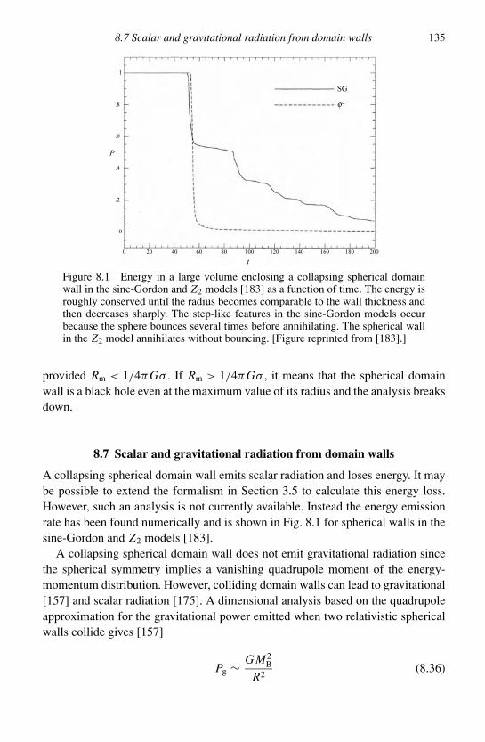
8.7 Scalar and gravitational radiation from domain walls 135
1
.8
.6
.4
.2
0
0 20 40 60 80 100
t
P
120 140 160 180
SG
f4
200
Figure 8.1 Energy in a large volume enclosing a collapsing spherical domainwall in the sine-Gordon and Z2 models [183] as a function of time. The energy isroughly conserved until the radius becomes comparable to the wall thickness andthen decreases sharply. The step-like features in the sine-Gordon models occurbecause the sphere bounces several times before annihilating. The spherical wallin the Z2 model annihilates without bouncing. [Figure reprinted from [183].]
provided Rm < 1/4πGσ . If Rm > 1/4πGσ , it means that the spherical domainwall is a black hole even at the maximum value of its radius and the analysis breaksdown.
8.7 Scalar and gravitational radiation from domain walls
A collapsing spherical domain wall emits scalar radiation and loses energy. It maybe possible to extend the formalism in Section 3.5 to calculate this energy loss.However, such an analysis is not currently available. Instead the energy emissionrate has been found numerically and is shown in Fig. 8.1 for spherical walls in thesine-Gordon and Z2 models [183].
A collapsing spherical domain wall does not emit gravitational radiation sincethe spherical symmetry implies a vanishing quadrupole moment of the energy-momentum distribution. However, colliding domain walls can lead to gravitational[157] and scalar radiation [175]. A dimensional analysis based on the quadrupoleapproximation for the gravitational power emitted when two relativistic sphericalwalls collide gives [157]
Pg ∼ G M2B
R2(8.36)
136 Gravity and cosmology of domain walls
where MB ∼ 4πσ R2 is the mass of the bubble and R is the radius upon collision.Numerical analyses of bubble collisions (during first-order phase transitions) foundthat the quadrupole approximation overestimates the power radiated in gravitationalradiation by about a factor of 50 [91].
8.8 Collapse into black holes
If the radius, R(t) of a collapsing spherical domain wall remains larger than theSchwarzschild radius, RS = 2G M , where M is the mass of the domain wall, thenthe domain wall does not become a black hole. As the wall collapses, it emitsscalar radiation and, if this is rapid enough, M decreases sufficiently rapidly sothat RS < R at all times. Whether this happens can be checked explicitly by nu-merical evolution of the scalar field plus Einstein equations. We expect that if theSchwarzschild radius of the spherical domain wall is smaller than the width of thewall, black holes are not formed since rapid wall annihilation and radiation precedecollapse to within the Schwarzschild radius.
The converse case of black hole formation in the case when the scalar radiationis not too rapid is harder to demonstrate convincingly. The reason is that the timeevolution of the fields gets slower as the black hole event horizon is about to form. Bysimply evolving the fields, it is impossible to see the formation of the event horizonand hence conclude that the domain wall collapses to form a black hole. However, itis hard to imagine any other outcome, especially since the scalar radiation rate onlybecomes significant once the spherical domain wall collapses to a size comparableto the thickness of the wall.
The collapse of a slightly perturbed spherical domain wall has been studiednumerically in [182] with the result that the amplitude of perturbations stays con-stant during the collapse. This means that the ratio of the perturbation amplitudeto the radius grows during collapse as 1/R(t) and the shape of the wall deviatesincreasingly from being spherical.
8.9 Cosmological domain walls: formation
The formation of domain walls in a phase transition in flat non-expanding space-time has been discussed in Chapter 6. Since the universe is expanding and cooling,cosmic phase transitions can occur, just as in the laboratory, and domain walls canalso form. If the phase transition proceeds quickly on cosmological time scales, thestructure of these domain wall networks is similar to those formed in the laboratoryand described in Chapter 6. The network is dominated by one infinite domain wallwith very complicated topology. However, if the phase transition occurs slowlyon cosmological time scales, the expansion can prevent the phase transition from
8.10 Cosmological domain walls: evolution 137
completion. For example, in a first-order phase transition, if the bubble nucleationrate is very slow, the bubbles will not be able to percolate because the expansionincreases the separation of the bubbles that have already nucleated. These consid-erations are important for inflationary cosmology but here we will assume that thephase transition completes since otherwise domain walls would not be formed.
In a model with 16πGη2 > 1 (η is the vacuum expectation value of the scalarfield), domain wall formation requires some new considerations [22, 166]. Thereason is that the energy density inside the domain walls is larger than that outside.Hence if such inflating domain walls (see Section 8.5) were to form, the space-timeexpansion rate within them would be greater than that of the ambient cosmologicalexpansion rate in which they were created. It is possible to show that a fasterexpanding region within a horizon of a slower expanding region can be createdonly if the null energy condition1 is violated. The formation of defects proceedsaccording to the classical dynamics of a scalar field with energy-momentum tensorgiven by Eq. (8.1). Contracting the energy-momentum tensor twice with a nullvector, Nµ, and using gµν NµN ν = 0 gives
NµN νTµν = (Nµ∂µφ)2 ≥ 0 (8.37)
Hence the null energy condition is satisfied during defect formation and there is anobstruction to the formation of topologically inflating domain walls. The exceptionis if the faster expanding region has an extent that is larger than the cosmologicalhorizon. In this situation, the domain wall is fatter than the horizon during thephase transition. Then the particle interaction rate is also slower than the Hubbleexpansion rate and the particles are not in a thermal state unless they were set upin that state as an initial condition at the Big Bang. The domain wall network thatis produced will depend on the initial state of the particles.
8.10 Cosmological domain walls: evolution
If we assume that there is a dense network of walls within our cosmological horizonand that the network does not lose a significant amount of energy to radiation, wecan work out the expansion rate of the universe and the scaling of the density ofwalls.
The energy-momentum of the scalar field that forms the domain walls is givenin Eq. (8.1). If we denote an average over a large volume by 〈·〉 we have
〈Tµν〉 = 〈∂µφ∂νφ〉 −⟨gµν
1
2(∂αφ)2 − V (φ)
⟩(8.38)
1 The null energy condition is Nµ N ν Tµν > 0 where Nµ is any null vector and Tµν is the energy-momentumtensor. For fluids with energy density ρ and isotropic pressure p, the null energy condition is ρ + p > 0.

138 Gravity and cosmology of domain walls
We assume that gµν is a background metric and only dependent on time. Also thefield distribution is assumed to be isotropic so that
〈(∂xφ)2〉 = 〈(∂yφ)2〉 = 〈(∂zφ)2〉 (8.39)
and
〈∂iφ∂ jφ〉 = 0, i = j (8.40)
Define
〈φ′2〉 = 1
3〈(∂xφ)2 + (∂yφ)2 + (∂zφ)2〉 (8.41)
If we further assume that the field is dominantly in the form of domain walls thatsatisfy Eq. (1.31) to a good approximation, we get
〈φ′2〉 = 2
3〈V 〉 (8.42)
which leads to
〈Txx〉 = 5
6〈φ2〉 − 2
3〈Ttt〉 (8.43)
For slowly varying fields this leads to the effective equation of state p = −2ρ/3where p is the (isotropic) pressure and ρ the energy density [186]. If we assumethat the time dependence of φ is only due to a boost of the domain walls, we canuse φ = vγ ∂Xφ = vγ
√2V (φ) and ∂xφ = γ ∂Xφ, where X = γ (x − vt) and γ is
the Lorentz factor (see Eq. (1.10)). This leads to
〈Txx〉 =(
〈v2〉 − 2
3
)〈Ttt〉 (8.44)
Following Appendix F and treating the wall network as a fluid with equationof state p = −2ρ/3, we can write down the solutions for the scale factor and thescaling of the energy density in walls. If the initial conditions are such that the walldensity is ρ0 when the scale factor is a0, the solution is
ρwalls(a) = ρ0a0
a, a(t) = a0
(t
t0
)2
(8.45)
Note that this derivation ignores processes by which the wall network could loseenergy into scalar and gravitational radiation. In addition, the walls interact withsurrounding matter and experience friction. These effects make the problem ofunderstanding the evolution of the wall network much more challenging. We nowdescribe some numerical [125, 36, 97, 59] and analytical [77, 78] efforts to under-stand the evolution of the network.
8.12 Evolution: analytical work 139
8.11 Evolution: numerical results
There are two numerical schemes for evolving a network of domain walls. Thefirst is to use the zero thickness approximation for walls. In this approximation, itis hard to treat the collision of walls and the loss of energy from the network intoradiation. The second approach is to solve the field theory equations of motion. Inthis approach, all the degrees of freedom of the system are retained. In fact, a lotof degrees of freedom that are evolved are inessential to the domain wall networkand this additional baggage slows down the simulations. In an expanding universethe problem is even more severe because the overall length scales grow larger withtime while the domain wall thickness remains the same. Thus the simulation needsto handle very disparate length scales.
In [125, 36, 97, 59], the authors get around these problems by solving the fieldtheory equations of motion but by letting the domain walls expand with the universe.
More specifically, consider the Z2 model in an expanding space-time with metric
gµν = a2(τ )ηµν (8.46)
where ηµν = diag(1, −1, −1, −1) and τ is the conformal time. The equation ofmotion is
∂2τ φ + 2
a
a∂τφ − ∇2φ + λ(φ2 − a2η2)φ = 0 (8.47)
In the approach pioneered in [125] the a2η2 in the last term is replaced by a constant,effectively decreasing the vacuum expectation value, η, with Hubble expansion.Since the width of the domain wall is proportional to 1/η, this amounts to lettingthe thickness of the walls grow in proportion to the scale factor.
The result of this numerical study shows that the areal density, A, i.e. area ofwalls in a given region divided by the volume of the region, scales inversely as thefirst power of conformal time
A = A0
(τ0
τ
)p, p ≈ 1 (8.48)
where the subscript 0 refers to some initial time. This result holds in Minkowskispace-time (a ∝ τ 0), radiation-dominated (a ∝ τ 1/2), and matter-dominated(a ∝ τ 1/3) cosmologies.
The domain wall network has also been studied by a combination of numericaland analytical techniques that use scaling arguments [13, 14].
8.12 Evolution: analytical work
An analytic technique to study the evolution of non-relativistic interfaces in thecondensed matter context was developed in [116] (also see [24, 65, 111]). The
140 Gravity and cosmology of domain walls
technique has been extended to relativistic systems in [77, 78] and we now sum-marize the main features of this analysis.
The starting point is to define a fictitious scalar field u(xµ) such that it vanisheson the domain wall network
u(Xµ(σ a)) = 0, a = 0, 1, 2 (8.49)
where the domain wall network is located at Xµ(σ a) and σ a denote world-volumecoordinates. While u(xµ) could have been taken to be the scalar field in the originalfield theory (say for the Z2 model), this is not suitable since u is later assumed to bea random field with a Gaussian distribution. The next step is to derive an equationof motion for u.
We define the domain wall world-volume metric as in Eq. (7.16)
hab = gµν(X )∂a Xµ∂b X ν (8.50)
where gµν is the ambient space-time metric and the indices a, b refer to world-volume coordinates. Two derivatives of Eq. (8.49) lead to
1√|h|∂a(√
|h|hab∂b Xµ)∂µu + hab∂a Xµ∂b X ν∂µ∂νu = 0 (8.51)
As long as the thin-wall limit is valid and, in particular, walls do not intersect,Xµ satisfies the Nambu-Goto equation. When walls do intersect, the Nambu-Gotoformalism breaks down. The formalism can continue to be valid provided we imposeadditional boundary conditions by hand at the intersection point. Depending onthe boundary conditions that one imposes at the intersection point, the Nambu-Goto equation can describe intercommuting walls or walls that pass through eachother. In the present formalism, the boundary conditions automatically arise fromthe evolution of the u field. The dynamics of the u field are such that they alwaysdescribe walls that intercommute [77]. Using the Nambu-Goto equations of motion,Eq. (7.21), then leads to the equation of motion for the fictitious field u
[(∂u)2gµν − ∂µu∂νu](∂µ∂νu − ρ
µν∂ρu) = 0 (8.52)
where ρµν is the Christoffel symbol defined in Eq. (7.22).
To solve Eq. (8.52) we must find a way to handle the non-linear terms. The keypoint now is that the domain wall network contains a random distribution of wallsand hence u is a statistical field. One approach to treat the non-linear terms is touse the mean field approximation. In this approach non-linear terms are replacedby averages of non-linear terms multiplied by a single power of u. For example
u3 → 〈u2〉u (8.53)
Further, the distribution of u is assumed to be Gaussian.
8.13 Cosmological constraints 141
After defining the correlators that enter the mean field theory version ofEq. (8.52), the field u satisfies the equation of motion
∂2τ u + µ(τ )
τ∂τ u − v2∇2u = 0 (8.54)
where, as in the previous section, τ is the conformal time, The functions µ andv2 are defined in terms of the assumed two-point correlation functions of u (fordetails see [77, 78]). Once the solution for u is obtained from the linear differentialequation, Eq. (8.54), the average areal density, A, and other quantities may becalculated. The results agree with the scaling in Eq. (8.48).
8.13 Cosmological constraints
The cosmological constraint on domain walls is remarkably robust, being almostindependent of the field theory, details of the phase transition, and cosmology [186].At any time after the domain wall forming phase transition, the vacua in differentcosmological horizons are uncorrelated. This means that there is at least one domainwall per horizon. The minimum area of a horizon size domain wall is ∼ H−2 whereH−1 is the horizon size. Therefore the domain wall energy density averaged overa horizon volume is ρwalls ∼ σ H . Comparing this to the critical density of theuniverse,2 we get
walls ≡ ρwalls
ρc∼ Gσ
H∼ Gσ t (8.55)
where t is the cosmic time. (We have taken H ∼ 1/t which is true in a Friedman-Robertson-Walker cosmology in which a(t) ∝ tα with 0 < α < 1.) Hence, as timeproceeds, there comes an epoch when the domain walls are the dominant form ofenergy in the universe. This happens at time t∗ given by
t∗ ∼ 1
Gσ(8.56)
Now σ ∼ η3 (e.g. Eq. (1.20)) up to factors of coupling constants which we assumeare order unity. We also know particle physics fairly well up to an energy scale ofabout 100 GeV (approximately the electroweak scale) and have not seen any scalarfields yet. So the minimum value of σ is about (100 GeV)3. Walls of this tensionwould have started dominating the universe at (see Appendix A for numericalvalues)
t∗
∣∣∣∣min
∼ m2P
η3∼ 108 s (8.57)
2 The critical density of the universe is defined as ρc = 3H2/8πG, where H (t) = a/a is the Hubble expansionrate defined in terms of the scale factor a(t) and its time derivative, a.

142 Gravity and cosmology of domain walls
or approximately 10 years after the Big Bang. Once the walls dominate, the universalexpansion becomes a ∝ t2 (Eq. (F.5)). This is unacceptable for several reasons. Forexample, since the domain wall dominated universe accelerates (a > 0), densityperturbations that are larger than the horizon keep getting stretched and stay largerthan the horizon. This means that super-horizon density perturbations can never re-enter the horizon, which is an essential condition for them to start growing to formthe galaxies, clusters, and large-scale structures that we currently observe. Eventhe growth of sub-horizon density perturbations is suppressed owing to cosmicacceleration.
A second constraint on a network of cosmic domain walls acting as a fluidwith equation of state p = −2ρ/3 comes from the measured expansion rate of theuniverse using supernovae data [127, 118]. These surveys find that the equationof state parameter, w ≡ p/ρ, for our universe is less than about −0.8 [11, 128].However, a universe dominated by a network of static (“frustrated”) domain walls[25] would have w ≈ −0.67.
Another possibility that has been considered is that perhaps there are somefeatures that are missing in the standard model of particle physics, and that thereindeed are very light domain walls in the universe [76]. Such light walls, if lightenough, would be benign and could potentially play a role in cosmology. If werequire that the domain walls not dominate the universe until the present time(∼ 1017 s), Eq. (8.57), gives η < 100 MeV. Other cosmological constraints, suchas arising from the isotropy of the cosmic microwave background can be used toput similar or somewhat stronger bounds on η [144, 158].
8.14 Constraints on and implications for particle physics
Let us summarize the picture that has emerged in this chapter.
If a field theory has discrete symmetries that are spontaneously broken in theground state, it must contain domain wall solutions.
If high-energy particle physics is described by such a field theory and the discretesymmetry gets spontaneously broken in the early universe, cosmic domain wallsare produced.
If the standard model is complete at energies below 100 GeV, then there can be nodomain walls in the universe and no spontaneously broken discrete symmetriesin particle physics.
A closer examination of this sequence of arguments reveals a few loopholes thatallow for spontaneously broken discrete symmetries in particle physics. First, thereis the possibility that the discrete symmetry was broken right from the moment ofthe Big Bang. Then the whole universe could have been in one of the many discretevacua at its very creation and no domain walls would be formed even though the

8.15 Metastable domain walls 143
D
V(f)
f2
f1
Figure 8.2 Sketch of the potential in the model of Eq. (8.58). Domain walls ariseowing to a 2π change in the angular field variable and the location of the fieldinside the wall is marked by D. Such domain walls can terminate on strings, andthe field within the string is located at φ = 0.
underlying particle-physics theory could have broken discrete symmetries. Thiskind of scenario has been studied for magnetic monopoles in [50]. A related possi-bility is that, if the universe went through a period of superluminal expansion (“in-flation”),3 then correlations extend to scales that are vastly larger than our currenthorizon and our region of the universe is very likely to be free of any domain walls[97]. In another variant, domain walls are formed but subsequently inflated away.
All the above loopholes only apply to very high-energy domain walls wherequantum gravity and/or inflation effects are relevant. If a particle-physics modelhas spontaneously broken discrete symmetries at lower energy scales (but still largerthan ∼ 100 MeV) no loopholes are known and the model is ruled out based on the“cosmological domain wall catastrophe.” However, there is still the possibility thatmetastable or biased domain walls (see Section 6.8) can exist for some time in theuniverse. We now describe these two possibilities.
8.15 Metastable domain walls
In certain field theories, it is possible for domain walls to get punctured. To see howthis can happen, consider the potential for a complex scalar field φ
V (φ) = λ
4(|φ|2 − η2)2 − αη
32(φ + φ∗)3 (8.58)
where we assume 0 < α << λ. The shape of this potential is shown in Fig. 8.2. Thefirst term is minimized when |φ| = η and, restricting φ to the submanifold |φ| = η,
3 Inflation occurs when the universe is dominated by a field that has an equation of state with −ρ < p < −ρ/3.Then the expansion rate of the universe is superluminal and volumes that are larger than the horizon can getcorrelated.

144 Gravity and cosmology of domain walls
StringDomain wall
Wall
String
Hole
χ = 0
χ = 2p χ = 0
Figure 8.3 Cross-section of a wall that terminates on a string is shown on theleft, and a wall with a puncture bordered by a string is shown on the right.
the second term is minimized when φ + φ∗ = +2η. Another way of writing thepotential is by setting φ = ψ exp(iχ ) and then ψ , χ are real fields. Then
V (φ) = λ
4(ψ2 − η2)2 − αη
4ψ3 cos3 χ (8.59)
The extrema of V are at ψ = 0 and at
ψ = η
[3α + √
9α2 + 64λ2
8λ
], χ = nπ (8.60)
where n is an integer. The true vacua occur when n is an even integer. For ex-ample, domain wall solutions exist with the boundary condition χ (x = −∞) = 0,χ (x = +∞) = 2π .
Now consider a domain wall in the model in 3 + 1 dimensions. Such a domainwall can terminate as shown in Fig. 8.3 since the path from χ = 0 to χ = 2π canbe contracted by lifting it over the top (ψ = 0) of the potential. While we havenot described cosmic strings here, in models such as Eq. (8.58), we can have finitesections of open walls that are bordered by strings. Walls can also get puncturedby holes that are bounded by strings. For further discussion of walls bounded bystrings, we refer the reader to [88, 168, 171].
The evolution of a network of walls that can have punctures is very differentfrom that of stable walls because a puncture can grow and eat up the wall. Thisprovides a very efficient way for the wall network to lose energy and so the networknever dominates the universe [168].
Another scheme that allows for the universe to have a finite period of time withdomain walls is if a discrete symmetry is broken and then restored (see Section 6.1).Walls would be formed at the first phase transition and then they would dissolve atthe second phase transition when the symmetry is restored. However, this scheme
8.15 Metastable domain walls 145
would imply an unbroken discrete symmetry in the low-energy particle physics.We do not know of such a discrete symmetry although the possibility cannot beexcluded.
Finally, domain walls could have existed for some time in the early universeif there is an approximate discrete symmetry in the high-energy particle-physicsmodel [60]. We have already seen an example of an approximate discrete symmetryin the SU (5) Grand Unification model discussed in Section 2.1. If the cubic couplingin the potential in Eq. (2.5) is small, it can be ignored and the resulting model hasSU (5) × Z2 symmetry, with all the domain wall solutions discussed in Section 2.2.A simpler example is that of the λφ4 together with a small cubic term. The potentialis
V (φ) = −m2
2φ2 + γ mφ3 + λ
4φ4 (8.61)
Now the model still has two local minima but they are not exactly degenerate if γ
is very small (see Fig. 6.11). At the phase transition, a network of domain walls isformed and the typical separation and curvature scale of the domain walls is givenby the correlation length ξ0. With time the curvature scale grows and is denoted byR(t). So the force per unit area on the wall owing to tension is ∼ σ/R(t) where σ isthe energy density of the wall. There is also a pressure difference pushing the walltoward the vacuum with the lowest energy. This pressure is given by the energydifference between the vacua and hence is proportional to γ
p ∼ γ mη3 (8.62)
where η is the vacuum expectation value of the field. Therefore the tension is muchlarger than the pressure, and the dynamics of the wall network are unaffected bythe pressure difference coming from the cubic term as long as
R(t) <σ
γ mη3∼ 1
γ η(8.63)
Once the network has evolved to a point where this condition is not met, the pressurebecomes important and drives the domain wall network such that the whole systemreaches the true vacuum. From the area scaling law in Eq. (8.48), it follows thatR(t) grows linearly with conformal time.4 Therefore, in a radiation dominateduniverse,
R = R0τ
τ0= R0
(t
t0
)1/2
(8.64)
4 The scaling law holds at late times after friction becomes unimportant. At earlier times, R grows as a differentpower of conformal time [87].
146 Gravity and cosmology of domain walls
where R0 can be taken to be the correlation length at the time of the phase transitiont0. Inserting this relation in Eq. (8.63) and using R0 ∼ 1/η, we get that the wallssurvive for a duration
twalls ∼ t0γ 2
(8.65)
If γ is small, the walls can survive for many Hubble expansions. In fact, if the wallssurvive for a long time, they might start dominating the density of the universebefore they disappear.
Even if domain walls are present in the universe for a relatively short time, theycan still have important implications for cosmology. As the wall network evolves,the ambient matter interacts with the walls. Magnetic monopoles can get trapped ondomain walls, leading to faster annihilation. This is the sweeping scenario discussedin [52]. In addition, the eventual collapse of domain walls can lead to black holeformation. These issues have received some attention but have yet to be studied indetail.
8.16 Open questions
1. What happens when a black hole collides with a domain wall? Does it get stuck on thewall? Or does it pass through? For a discussion from the gravitational point of view, see[29, 148].
2. Develop an analytical formulation (perhaps along the lines of Section 3.5) to calculatethe scalar radiation rate from collapsing domain walls.
3. Discuss the cosmology of superconducting domain walls.4. What is the outcome of the SU (5) Grand Unified phase transition when the cubic coupling
is small? Are domain walls formed? How does the network evolve?

9
Kinks in the laboratory
In this chapter we discuss two laboratory systems where kinks are known to exist.The first system is trans polyacetylene which has a broken Z2 symmetry as in theλφ4 model. The second system is a Josephson junction transmission line, which isa laboratory realization of the sine-Gordon system. Helium-3 is another laboratorysystem that contains a wide variety of topological defects and the reader is referred to[174] for a discussion. In the third section of this chapter we describe Scott Russell’ssolitons in water. These solitons are not topological like the others discussed in thisbook but we include the discussion anyway since the reader’s curiosity may havebeen aroused by the story in the Preface.
9.1 Polyacetylene
Polyacetylene consists of a linear chain of CH bonds. A sequence of x units iswritten as (CH)x . In the ground state of polyacetylene, the carbon atom forms threeσ bonds, one of them is to the H in the CH unit, one to the unit on the left and oneto the right. In addition, there is one more electron orbital that can cause bonding.This is called the π electron, and the π bond can form to the left or to the right.Then there are two possible sequences – first when the double (σ and π ) bond isto the carbon on the right and the single to the left, the second when the doublebond is to the left and the single to the right. These two possibilities are illustratedin Fig. 9.1 [149] in the trans configuration of polyacetylene.1
The average bond length a ≈ 1.22 A but the CH units are displaced so as to makedouble bonds (slightly) shorter than the single bonds. The physical displacements un
along the horizontal axis in the two structures are depicted in Fig. 9.1. Qualitatively,the essential point is that the π electrons have to choose to either form the double
1 In the cis configuration, there are also two states related by the left-right transformation but they are not degeneratein energy.
147
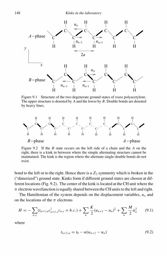
148 Kinks in the laboratory
C
H
C
H
C
H
C
H
C
H
C
H
C
H
C
H
C
H
C
H
C
H
C
H
C
H
C
H
2a
un−1 un+1
A −phase
B −phase C
H
C
H
C
H
C
Hun+1un−1
un
un
y
x
Figure 9.1 Structure of the two degenerate ground states of trans polyacetylene.The upper structure is denoted by A and the lower by B. Double bonds are denotedby heavy lines.
C
H
C
H
C
H
C
H
C
H
C
H
C
H
C
H
C
H
C
H
C
H
C
H
C
H
C
H
C
H
C
H
C
H
B−phase A − phase
Figure 9.2 If the B state occurs on the left side of a chain and the A on theright, there is a kink in between where the simple alternating structure cannot bemaintained. The kink is the region where the alternate single-double bonds do notexist.
bond to the left or to the right. Hence there is a Z2 symmetry which is broken in the(“dimerized”) ground state. Kinks form if different ground states are chosen at dif-ferent locations (Fig. 9.2). The center of the kink is located at the CH unit where theπ electron wavefunction is equally shared between the CH units to the left and right.
The Hamiltonian of the system depends on the displacement variables, un andon the locations of the π electrons
H = −∑n,s
(tn+1,nc†n+1,scn,s + h.c.) +∑
n
K
2(un+1 − un)2 +
∑n
M
2u2
n (9.1)
where
tn+1,n = t0 − α(un+1 − un) (9.2)
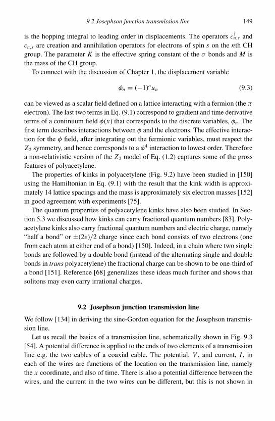
9.2 Josephson junction transmission line 149
is the hopping integral to leading order in displacements. The operators c†n,s andcn,s are creation and annihilation operators for electrons of spin s on the nth CHgroup. The parameter K is the effective spring constant of the σ bonds and M isthe mass of the CH group.
To connect with the discussion of Chapter 1, the displacement variable
φn = (−1)nun (9.3)
can be viewed as a scalar field defined on a lattice interacting with a fermion (the π
electron). The last two terms in Eq. (9.1) correspond to gradient and time derivativeterms of a continuum field φ(x) that corresponds to the discrete variables, φn . Thefirst term describes interactions between φ and the electrons. The effective interac-tion for the φ field, after integrating out the fermionic variables, must respect theZ2 symmetry, and hence corresponds to a φ4 interaction to lowest order. Thereforea non-relativistic version of the Z2 model of Eq. (1.2) captures some of the grossfeatures of polyacetylene.
The properties of kinks in polyacetylene (Fig. 9.2) have been studied in [150]using the Hamiltonian in Eq. (9.1) with the result that the kink width is approxi-mately 14 lattice spacings and the mass is approximately six electron masses [152]in good agreement with experiments [75].
The quantum properties of polyacetylene kinks have also been studied. In Sec-tion 5.3 we discussed how kinks can carry fractional quantum numbers [83]. Poly-acetylene kinks also carry fractional quantum numbers and electric charge, namely“half a bond” or ±(2e)/2 charge since each bond consists of two electrons (onefrom each atom at either end of a bond) [150]. Indeed, in a chain where two singlebonds are followed by a double bond (instead of the alternating single and doublebonds in trans polyacetylene) the fractional charge can be shown to be one-third ofa bond [151]. Reference [68] generalizes these ideas much further and shows thatsolitons may even carry irrational charges.
9.2 Josephson junction transmission line
We follow [134] in deriving the sine-Gordon equation for the Josephson transmis-sion line.
Let us recall the basics of a transmission line, schematically shown in Fig. 9.3[54]. A potential difference is applied to the ends of two elements of a transmissionline e.g. the two cables of a coaxial cable. The potential, V , and current, I , ineach of the wires are functions of the location on the transmission line, namelythe x coordinate, and also of time. There is also a potential difference between thewires, and the current in the two wires can be different, but this is not shown in
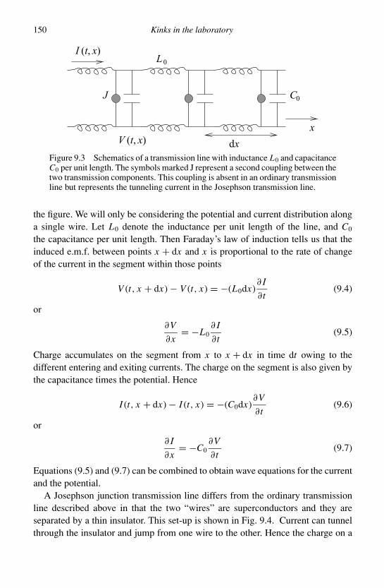
150 Kinks in the laboratory
I (t, x)
V (t, x)
J
L 0
C0
x
dxFigure 9.3 Schematics of a transmission line with inductance L0 and capacitanceC0 per unit length. The symbols marked J represent a second coupling between thetwo transmission components. This coupling is absent in an ordinary transmissionline but represents the tunneling current in the Josephson transmission line.
the figure. We will only be considering the potential and current distribution alonga single wire. Let L0 denote the inductance per unit length of the line, and C0
the capacitance per unit length. Then Faraday’s law of induction tells us that theinduced e.m.f. between points x + dx and x is proportional to the rate of changeof the current in the segment within those points
V (t, x + dx) − V (t, x) = −(L0dx)∂ I
∂t(9.4)
or
∂V
∂x= −L0
∂ I
∂t(9.5)
Charge accumulates on the segment from x to x + dx in time dt owing to thedifferent entering and exiting currents. The charge on the segment is also given bythe capacitance times the potential. Hence
I (t, x + dx) − I (t, x) = −(C0dx)∂V
∂t(9.6)
or
∂ I
∂x= −C0
∂V
∂t(9.7)
Equations (9.5) and (9.7) can be combined to obtain wave equations for the currentand the potential.
A Josephson junction transmission line differs from the ordinary transmissionline described above in that the two “wires” are superconductors and they areseparated by a thin insulator. This set-up is shown in Fig. 9.4. Current can tunnelthrough the insulator and jump from one wire to the other. Hence the charge on a
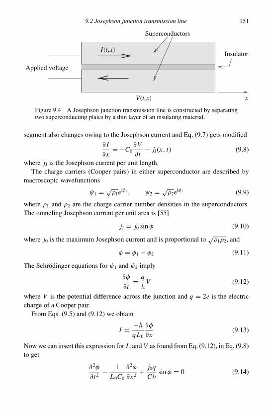
9.2 Josephson junction transmission line 151
Superconductors
InsulatorI(t,x)
V(t,x) x
Applied voltage
Figure 9.4 A Josephson junction transmission line is constructed by separatingtwo superconducting plates by a thin layer of an insulating material.
segment also changes owing to the Josephson current and Eq. (9.7) gets modified
∂ I
∂x= −C0
∂V
∂t− jJ(x, t) (9.8)
where jJ is the Josephson current per unit length.The charge carriers (Cooper pairs) in either superconductor are described by
macroscopic wavefunctions
ψ1 = √ρ1eiφ1, ψ2 = √
ρ2eiφ2 (9.9)
where ρ1 and ρ2 are the charge carrier number densities in the superconductors.The tunneling Josephson current per unit area is [55]
jJ = j0 sin φ (9.10)
where j0 is the maximum Josephson current and is proportional to√
ρ1ρ2, and
φ = φ1 − φ2 (9.11)
The Schrodinger equations for ψ1 and ψ2 imply
∂φ
∂t= q
V (9.12)
where V is the potential difference across the junction and q = 2e is the electriccharge of a Cooper pair.
From Eqs. (9.5) and (9.12) we obtain
I = −
q L0
∂φ
∂x(9.13)
Now we can insert this expression for I , and V as found from Eq. (9.12), in Eq. (9.8)to get
∂2φ
∂t2− 1
L0C0
∂2φ
∂x2+ j0q
Csin φ = 0 (9.14)

152 Kinks in the laboratory
Rescaling t and x by the Josephson time and length scales
τ =(
C0
q J0
)1/2
, l =(
q J0L0
)1/2
(9.15)
gives the sine-Gordon equation as derived from Eq. (1.51) with α = 1 = β.
9.3 Solitons in shallow water
The solitons discussed in this book have all had a topological origin. In contrast,the solitons first discovered by Scott Russell in a water channel, and mentioned inthe Preface, have their origin in the non-linearities of hydrodynamics and do nothave a topological origin.
The first step to show the existence of the water solitons is to derive the Korteweg-deVries (KdV) equation for waves of long wavelength moving in one direction inshallow water. We do not give this derivation here and instead refer the reader to,for example, Section 13.11 of [180].
The KdV equation is
∂u
∂t+ u
∂u
∂x+ δ2 ∂3u
∂x3= 0 (9.16)
where u is related to the height of the fluid surface and δ is a parameter. The solitonsolution is [185]
u = u∞ + (u0 − u∞)sech2
[X − X0
](9.17)
where X = x − vt , X0 is a constant, v is the velocity of the soliton,
= δ
[u0 − u∞
12
]−1/2
(9.18)
The velocity of the soliton is given by
v = u∞ + u0 − u∞3
(9.19)
in terms of the arbitrary constants u0 and u∞. Note that the amplitude of the solitonand the velocity are related.
9.4 Concluding remarks
There are a number of situations where solitons have been discussed in the par-ticle physics literature. Most of these discussions, such as of domain walls in theSU (5) × Z2 model in Chapter 2, have been in the framework of Grand Unified
9.5 Open questions 153
Theories. The attention has mostly focused on magnetic monopoles and stringsbecause monopoles seem inevitable in this class of theories and strings are lessconstrained by cosmology. Similar topological structures also exist in the standardmodel of electroweak interactions but the monopoles are confined and the stringsare unstable [2]. Domain wall and string solutions also exist in QCD in variousexternal conditions, for example in high density matter such as might be presentin the interiors of neutron stars [142]. Unlike solitons in the laboratory, however,solitons in particle physics and cosmology have not yet been discovered experi-mentally. Given the very similar underpinnings of laboratory and particle physicssystems, there is hope that this situation will soon change.
9.5 Open questions
1. Is there a condensed matter system with spontaneously broken permutation symmetry?Discuss the domain walls in that system and whether a lattice can exist. Can the wallsbe observed experimentally?
2. If there are QCD domain walls in neutron stars, how might they be observed from Earth?
Appendix A
Units, numbers and conventions
We will work in natural units in which = c = 1. In these units, all dimensionfulquantities have dimensions of mass to some power. One way to convert from mass (g) tolength (cm) and time (s), is to remember the values for the Planck mass, time, and length:mP = 1.2 × 10¹⁹ GeV, tP = 5.4 × 10−43 s, lP = 1.6 × 10⁻³³ cm. Also, mPtP = 1 = mPlPin natural units. It is also useful to remember mP = 2.2 × 10⁻⁵ g and, when dealing withmagnetic fields, the conversion: 1 Gauss = 1.95 × 10⁻²⁰ GeV2. In addition, forcosmological estimates it is convenient to know that 1 pc = 3.1 × 1018 cm.
The metric signature is taken to be (+, −, −, −).
154
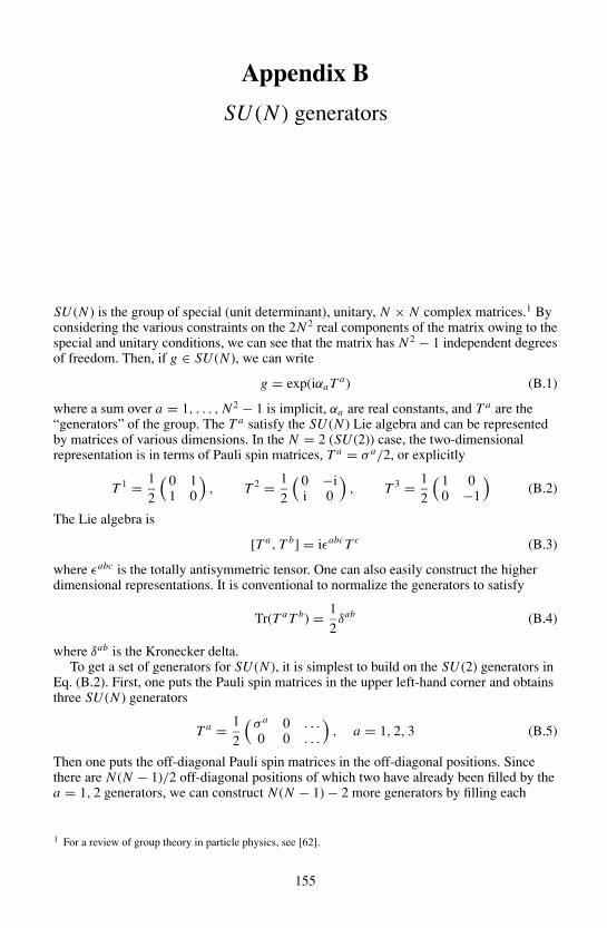
Appendix B
SU (N ) generators
SU (N ) is the group of special (unit determinant), unitary, N × N complex matrices.1 Byconsidering the various constraints on the 2N 2 real components of the matrix owing to thespecial and unitary conditions, we can see that the matrix has N 2 − 1 independent degreesof freedom. Then, if g ∈ SU (N ), we can write
g = exp(iαa T a) (B.1)
where a sum over a = 1, . . . , N 2 − 1 is implicit, αa are real constants, and T a are the“generators” of the group. The T a satisfy the SU (N ) Lie algebra and can be representedby matrices of various dimensions. In the N = 2 (SU (2)) case, the two-dimensionalrepresentation is in terms of Pauli spin matrices, T a = σ a/2, or explicitly
T 1 = 1
2
( 0 11 0
), T 2 = 1
2
( 0 −ii 0
), T 3 = 1
2
( 1 00 −1
)(B.2)
The Lie algebra is
[T a, T b] = iεabcT c (B.3)
where εabc is the totally antisymmetric tensor. One can also easily construct the higherdimensional representations. It is conventional to normalize the generators to satisfy
Tr(T a T b) = 1
2δab (B.4)
where δab is the Kronecker delta.To get a set of generators for SU (N ), it is simplest to build on the SU (2) generators in
Eq. (B.2). First, one puts the Pauli spin matrices in the upper left-hand corner and obtainsthree SU (N ) generators
T a = 1
2
(σ a 0 . . .0 0 . . .
), a = 1, 2, 3 (B.5)
Then one puts the off-diagonal Pauli spin matrices in the off-diagonal positions. Sincethere are N (N − 1)/2 off-diagonal positions of which two have already been filled by thea = 1, 2 generators, we can construct N (N − 1) − 2 more generators by filling each
1 For a review of group theory in particle physics, see [62].
155

156 SU (N ) generators
remaining position by either 1 (as in σ 1) or by ±i (as in σ 2). These look like
1
2
0 0 . . . . . . . . .0 0 . . . . . . . . .. . . . 1 jk0 . . . 1k j. . . . . . . . . . . . . . .
,
1
2
0 0 . . . . . .0 0 . . . . . . . . .. . . . −i jk0 . . . ik j . . .. . . . . . 0 . . . . . .
(B.6)
where the subscripts j , k denote the position in the matrix.Finally we construct the diagonal generators. These are written by putting a series of 1s
in say, n, successive diagonal positions, and then entering −n in the nn entry of thematrix. This scheme ensures that the generator is traceless and the resulting matrix is
diag(1, . . . , 1n, −n, 0, . . . , 0) (B.7)
where 1n denotes 1 in the nn entry. The normalization is then fixed using the convention inEq. (B.4) to get the generator
1√2n(n + 1)
diag(1, . . . , 1n, −n, 0, . . . , 0) (B.8)
In this way we construct N − 1 diagonal generators, one for each value of n. The thirdPauli matrix is already included as the a = 3 generator.
As a check, we find that the total number of generators constructed is3 + (N (N − 1) − 2) + (N − 2) = N 2 − 1 and this agrees with the degrees of freedom inSU (N ).
In the SU (5) Grand Unified model discussed in Chapter 2 an alternate set of diagonalgenerators is useful.
λ3 = 1
2diag(1, −1, 0, 0, 0)
λ8 = 1
2√
3diag(1, 1, −2, 0, 0)
τ3 = 1
2diag(0, 0, 0, 1, −1)
Y = 1
2√
15diag(2, 2, 2, −3, −3)
After the SU (5) symmetry is broken by the canonical vacuum expectation value of (Eq. (2.6)), λ3 and λ8 are generators of the unbroken SU (3), τ3 of SU (2), and Y of U (1).

Appendix C
Solution to a common differential equation
We have often encountered a differential equation of the type
−d2ψ
dx2+ [ε − v cosh 2µ − v sinh 2µ tanh x + v cosh2 µ sech2x
]ψ = 0 (C.1)
where v, µ are parameters and ε is the eigenvalue. This differential equation has beensolved in Section 12.3 of [113] where the Schrodinger problem has also been extensivelystudied. Here we reproduce the solution.
The solution is given in terms of new parameters a and b
a = 1
2
√ve2µ − ε − 1
2
√ve−2µ − ε ≡ 1
2κ+ − 1
2κ− (C.2)
b = 1
2
√ve2µ − ε + 1
2
√ve−2µ − ε ≡ 1
2κ+ + 1
2κ− (C.3)
Then, with
ψ = e−ax sechbx F(x) (C.4)
the equation for F becomes
F ′′ − 2[a + b tanh x]F ′ + [v cosh2 µ − b(b + 1)]sech2x F = 0 (C.5)
where primes denote derivatives with respect to x . Defining
u = 1
2[1 − tanh x] (C.6)
we get the hypergeometric equation
u(1 − u)d2 F
du2+ [a + b + 1 − 2(b + 1)u]
dF
du+ [v cosh2 µ − b(b + 1)]F = 0 (C.7)
The general solution may be found in [71]
F = AF1 + B F2 (C.8)
where A and B are constants of integration and
F1 = F(α, β; γ ; u) (C.9)
F2 = u1−γ F(α − γ + 1, β − γ + 1; 2 − γ ; u) (C.10)
157
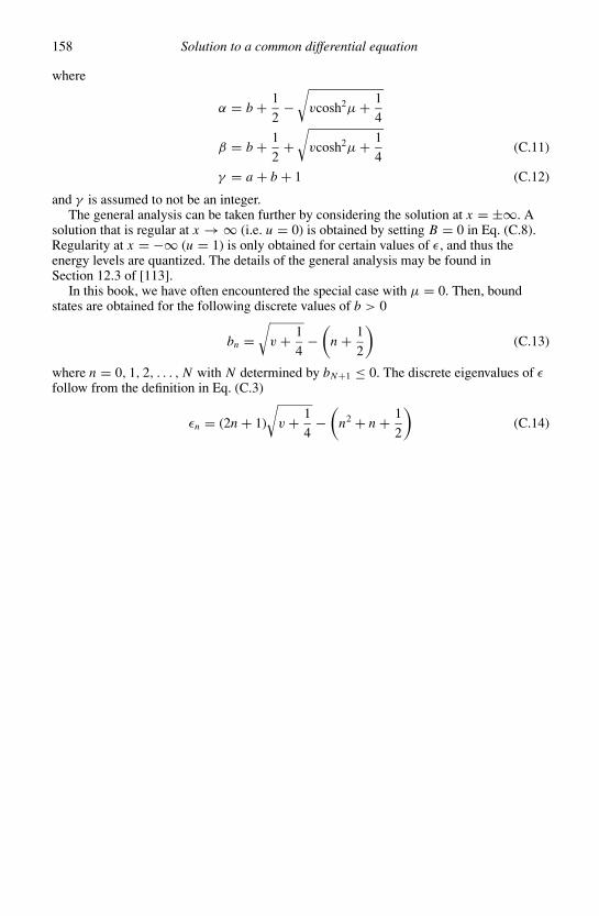
158 Solution to a common differential equation
where
α = b + 1
2−√
vcosh2µ + 1
4
β = b + 1
2+√
vcosh2µ + 1
4(C.11)
γ = a + b + 1 (C.12)
and γ is assumed to not be an integer.The general analysis can be taken further by considering the solution at x = ±∞. A
solution that is regular at x → ∞ (i.e. u = 0) is obtained by setting B = 0 in Eq. (C.8).Regularity at x = −∞ (u = 1) is only obtained for certain values of ε, and thus theenergy levels are quantized. The details of the general analysis may be found inSection 12.3 of [113].
In this book, we have often encountered the special case with µ = 0. Then, boundstates are obtained for the following discrete values of b > 0
bn =√
v + 1
4−(
n + 1
2
)(C.13)
where n = 0, 1, 2, . . . , N with N determined by bN+1 ≤ 0. The discrete eigenvalues of εfollow from the definition in Eq. (C.3)
εn = (2n + 1)
√v + 1
4−(
n2 + n + 1
2
)(C.14)
Appendix D
Useful operator identities
Identity 1
We wish to prove1
eA+B = eAeBeC/2 (D.1)
where C = [B, A] is assumed to commute with A and B.Let
S(x) = e(A+B)x (D.2)
where x is a parameter. Write
S(x) = eAxU (x) (D.3)
where U is an unknown matrix-valued function. Then
(A + B)S(x) = dS
dx= AeAxU (x) + eAx dU
dx(D.4)
which leads todU
dx= e−Ax Be+AxU (x) (D.5)
Now
BeAx = B∑
n
(Ax)n
n!=∑
n
(Ax)n
n!B +
∑n
[B, An]xn
n!(D.6)
Also,
[B, An] = An−1[B, A] + [B, An−1]A = · · · = [B, A]n An−1 (D.7)
provided C = [B, A] commutes with A. Therefore
BeAx = eAx B + [B, A]xeAx (D.8)
anddU
dx= (B + [B, A]x)U (x) (D.9)
1 Several of the proofs in this Appendix were provided by Harsh Mathur, private communication (2005).
159
160 Useful operator identities
This equation can be solved to get
U (x) = exp(Bx + [B, A]x2/2) (D.10)
This solution satisfies the boundary condition U (0) = 1.Hence
S(x) = e(A+B)x = eAx eBx e[B,A]x2/2 (D.11)
With x = 1, we get the desired result.
Identity 2
Here we outline a proof of the identity
: eA+B :=: eA :: eB : eD (D.12)
where D = [A+, B−] is assumed to be a c-number. Also, a linear decomposition of A andB is assumed A = A+ + A−, B = B+ + B− and the superscripts ± refer to termsproportional to creation (+) and annihilation (−) operators. Expressions sandwichedbetween : : are normal ordered, and so annihilation operators are placed to the right ofcreation operators.
The first step is the identity
: eA := eA−eA+
(D.13)
This can be proved by explicit expansion of the exponentials.Then
: eA :: eB := eA−eA+
eB−eB+
(D.14)
and
: eA+B := eA−eB−
eA+eB+
(D.15)
since [A−, B−] = 0 = [A+, B+].Now we use the identity, Eq. (D.1) proved in the previous section to exchange the order
of the middle two factors in Eq. (D.14) and together with Eq. (D.15) gives the identity inEq. (D.12).
Identity 3
Here we wish to show
A : eB :=: A + [A+, B−]eB : (D.16)
A : eB : =∞∑
n=0
(A+ + A−)
n!
n∑k=0
n!
k!(n − k)!(B−)k(B+)n−k (D.17)
=∞∑
n=0
1
n!
n∑k=0
n!
k!(n − k)!(B−)k A+ + [A+, (B−)k]
+A−(B−)k (B+)n−k (D.18)
Useful operator identities 161
Now use
[A+, (B−)k] = k(B−)k−1[A+, B−] (D.19)
provided that [A+, B−] is a c-number. Therefore
A : eB : =∞∑
n=0
1
n!
n∑k=0
n!
k!(n − k)!(B−)k A+ + k(B−)k−1[A+, B−]
+A−(B−)k (B+)n−k (D.20)
= : (A + [A+, B−])eB : (D.21)
Similarly we can show
: eB : A =: eB(A + [B+, A−]) : (D.22)
Putting this together with Eq. (D.16) we get
[A, : eB :] =: [A, eB] : +([A+, B−] − [B+, A−]) : eB : (D.23)
In the case of interest for deriving Eq. (4.80) we have
A+ = (A−)†, B+ = −(B−)† (D.24)
then
[A+, B−] − [B+, A−] = [A+, B−] + [A+, B−]† (D.25)
With A = φ(y) and : eB := ψ(x), [A+, B−] is purely imaginary and the right-hand sidevanishes. Then Eq. (D.23) gives the identity
[A, : eB :] =: [A, eB] : (D.26)

Appendix E
Variation of the determinant
If M is a matrix function and δM is a small variation of M , we wish to find the variationof the determinant of M (we follow Section 4.7 of [177]).
Consider
δ[ln(DetM(x))] = ln(Det(M + δM)) − ln(Det(M))
= ln
[Det(M + δM)
Det(M)
]
= ln(DetM−1Det(M + δM))
= ln(DetM−1(M + δM))= ln(Det1 + M−1δM)= ln(1 + TrM−1δM) + O((δM)2)
= TrM−1δM + O((δM)2) (E.1)
Hence
δ[(DetM(x))] = Tr[M−1(x)δM(x)]DetM(x) (E.2)
which is the desired result.
162
Appendix F
Summary of cosmological equations
Assuming an isotropic and homogeneous universe, the cosmological line element is theFriedman-Robertson-Walker line element, and can be written as:
ds2 = dt2 − a2(t)
[dr2
1 − kr2+ r2(dθ2 + sin2 θdφ2)
](F.1)
The function a(t) is known as the scale factor. k is a parameter that is −1 for a hyperbolicor negatively curved universe, 0 for a flat universe, and +1 for a positively curveduniverse.
The equations of motion for a are derived from Einstein’s equations assuming that theuniverse is filled with one or more fluids1 with total energy density ρ and pressure p.Then:
H 2 ≡(
a
a
)2
= 8πG
3ρ − k
a2(F.2)
a = −4πG
3(ρ + 3p)a (F.3)
and energy-momentum conservation gives:
d
da(ρa3) = −3pa2 (F.4)
In addition, we need the equation of state for the fluid to connect p and ρ. Some examplesof equations of state are: p = −ρ (cosmological constant), p = 0 (dust), p = ρ/3(radiation), and p = −2ρ/3 (slowly evolving wall network). Note that ρ may containcontributions from a large variety of forms of matter and then the corresponding energydensities and pressures must be added together.
1 The fluid approximation means that the relaxation time of the various components – which in our case maybe plasma, gas, stars, galaxies, walls, fundamental particles – is much shorter than the characteristic time forchanges in the scale factor.
163
164 Summary of cosmological equations
Assuming a single dominant component of energy density in a flat universe (k = 0),Eqs. (F.2) and (F.4) can be solved to obtain:
p = −ρ → a ∝ eHt , ρ ∝ a0
p = 0 → a ∝ t2/3, ρ ∝ 1
a3
p = ρ
3→ a ∝ t1/2, ρ ∝ 1
a4
p = −2
3ρ → a ∝ t2, ρ ∝ 1
a(F.5)
p = wρ → a ∝ t2/3(w+1), ρ ∝ a−3(w+1) (F.6)

References
[1] Ablowitz, M. J. and Clarkson, P. A., Solitons, Nonlinear Evolution Equations andInverse Scattering. London Mathematical Society 149 (Cambridge: CambridgeUniversity Press, 1991).
[2] Achucarro, A. and Vachaspati, T., Semilocal and electroweak strings. Phys. Rep.,327 (2000), 347. [Phys. Rep., 327 (2000), 427] [arXiv:hep-ph/9904229].
[3] Actor, A., Classical solutions of SU(2) Yang-Mills theories. Rev. Mod. Phys., 51(1979), 461.
[4] Anninos, P., Oliveira, S. and Matzner, R. A., Fractal structure in the scalar lambda(φ2 − 1)2 theory. Phys. Rev., D44 (1991), 1147.
[5] Antunes, N. D., Bettencourt, L. M. A. and Hindmarsh, M., The thermodynamics ofcosmic string densities in U(1) scalar field theory. Phys. Rev. Lett., 80 (1998), 908.[arXiv:hep-ph/9708215].
[6] Antunes, N. D., Pogosian, L. and Vachaspati, T., On formation of domain walllattices. Phys. Rev., D69 (2004), 043513. [arXiv:hep-ph/0307349].
[7] Antunes, N. D. and Vachaspati, T., Spontaneous formation of domain wall lattices intwo spatial dimensions. Phys. Rev., D70 (2004), 063516. [arXiv:hep-ph/0404227].
[8] Antunes, N. D., Gandra, P. and Rivers, R. J., Domain formation: decided before, orafter the transition? (2005) [hep-ph/0504004].
[9] Arodz, H., Expansion in the width and collective dynamics of a domain wall. Nucl.Phys., B509 (1997), 273. [arXiv:hep-th/9703168].
[10] Arodz, H., Dziarmaga, J. and Zurek, W. H., Patterns of Symmetry Breaking(Dordrecht: Kluwer Academic Publishers, 2003).
[11] Astier, P., Guy, J., Regnault, N., et al. The supernova legacy survey: measurementof M , and w from the first year data set. (2005) [astro-ph/0510447].
[12] Atiyah, M. F., Hitchin, N. J., Drinfeld, V. G. and Manin, Y. I., Construction ofinstantons. Phys. Lett., A65 (1978), 185.
[13] Avelino, P. P., Oliveira, J. C. R. and Martins, C. J. A., Understanding domain wallnetwork evolution. Phys. Lett., B610 (2005), 1. [arXiv:hep-th/0503226].
[14] Avelino, P. P., Martins, C. J. A. and Oliveira, J. C. R., One-scale model for domainwall network evolution. Phys. Rev., D72 (2005), 083506. [arXiv:hep-ph/0507272].
[15] Barr, S. M. and Matheson, A. M., Weak resistance in superconducting cosmicstrings. Phys. Rev., D36 (1987), 2905.
[16] Basu, R., Guth, A. H. and Vilenkin, A., Quantum creation of topological defectsduring inflation. Phys. Rev., D44 (1991), 340.
165

166 References
[17] Basu, R. and Vilenkin, A., Nucleation of thick topological defects during inflation.Phys. Rev., D46 (1992), 2345.
[18] Basu, R. and Vilenkin, A., Evolution of topological defects during inflation.Phys. Rev., D50 (1994), 7150. [arXiv:gr-qc/9402040].
[19] Bogolubsky, I. L. and Makhanov, V. G., Lifetime of pulsating solitons in certainclassical models. JETP Lett., 24 (1976), 12.
[20] Bogomolnyi, E. B., The stability of classical solutions. Sov. J. Nucl. Phys.,24 (1976), 449.
[21] Bonjour, F., Charmousis, C. and Gregory, R., The dynamics of curved gravitatingwalls. Phys. Rev., D62 (2000), 083504. [arXiv:gr-qc/0002063].
[22] Borde, A., Trodden, M. and Vachaspati, T., Creation and structure of baby universesin monopole collisions. Phys. Rev., D59 (1999), 043513. [arXiv:gr-qc/9808069].
[23] Boys, C. V., Soap Bubbles: Their Colors and Forces Which Mold Them (New York:Dover Publications, 1959).
[24] Bray, A., Topological defects and phase ordering dynamics. In Formation andInteraction of Topological Defects, ed. A.-C. Davis and R. Brandenberger(New York: NATO ASI Series, Plenum, 1995).
[25] Bucher, M. and Spergel, D. N., Is the dark matter a solid? Phys. Rev., D60 (1999),043505. [arXiv:astro-ph/9812022].
[26] Campbell, D. K., Schonfeld, J. F. and Wingate, C. A., Resonance structure inkink-antikink interactions in phi**4 theory. Physica, 9D (1983), 1.
[27] Caroli, C., de Gennes, P. G. and Matricon, J., Bound fermion states on a vortex linein a type II superconductor. Phys. Lett., 9 (1964), 307.
[28] Carter, B. and Gregory, R., Curvature corrections to dynamics of domain walls.Phys. Rev., D51 (1995), 5839. [arXiv:hep-th/9410095].
[29] Chamblin, A. and Eardley, D. M., Puncture of gravitating domain walls. Phys. Lett.,B475 (2000), 46. [arXiv:hep-th/9912166].
[30] Cheng, T. P. and Li, L. F., Gauge Theory of Elementary Particle Physics (New York:Oxford University Press, 1984).
[31] Cho, I. and Vilenkin, A., Spacetime structure of an inflating global monopole.Phys. Rev., D56 (1997), 7621. [arXiv:gr-qc/9708005].
[32] Ciria, J. C. and Tarancon, A., Renormalization group study of the soliton mass inthe (1 + 1)-dimensional λφ4 lattice model. Phys. Rev., D49 (1994), 1020.[arXiv:hep-lat/9309019].
[33] Coleman, S. R. and Weinberg, E., Radiative corrections as the origin of spontaneoussymmetry breaking. Phys. Rev., D7 (1973), 1888.
[34] Coleman, S. R., Quantum sine-Gordon equation as the massive Thirring model.Phys. Rev., D11 (1975), 2088.
[35] Coleman, S., Aspects of Symmetry (Cambridge: Cambridge University Press,1985).
[36] Coulson, D., Lalak, Z. and Ovrut, B. A., Biased domain walls. Phys. Rev.,D53 (1996), 4237.
[37] Creutz, M., Quarks, Gluons and Lattices (Cambridge: Cambridge University Press,1985).
[38] Dashen, R. F., Hasslacher, B. and Neveu, A., Nonperturbative methods andextended hadron models in field theory. 1. Semiclassical functional methods.Phys. Rev., D10 (1974), 4114.
[39] Dashen, R. F., Hasslacher, B. and Neveu, A., Nonperturbative methods andextended hadron models in field theory. 2. Two-dimensional models and extendedhadrons. Phys. Rev., D10 (1974), 4130.

References 167
[40] Dashen, R. F., Hasslacher, B. and Neveu, A., Nonperturbative methods andextended hadron models in field theory. 3. Four-dimensional nonabelian models.Phys. Rev., D10 (1974), 4138.
[41] Dashen, R. F., Hasslacher, B. and Neveu, A., The particle spectrum in model fieldtheories from semiclassical functional integral techniques. Phys. Rev., D11 (1975),3424.
[42] Dashen, R. F., Hasslacher, B. and Neveu, A., Semiclassical bound states in anasymptotically free theory. Phys. Rev., D12 (1975), 2443.
[43] Davidson, A., Toner, B. F., Volkas, R. R. and Wali, K. C., Clash of symmetries onthe Brane. Phys. Rev., D65 (2002), 125013. [arXiv:hep-th/0202042].
[44] von Delft, J. and Schoeller, H., Bosonization for beginners: Refermionization forexperts. Ann. Phys., 7 (1998), 225. [arXiv:cond-mat/9805275].
[45] Derrick, G. H., Comments on nonlinear wave equations as models for elementaryparticles. J. Math. Phys., 5 (1964), 1252.
[46] Deser, S., Plane waves do not polarize the vacuum. J. Phys. A, Math. Gen.,8 (1975), 1972.
[47] Dolan, L. and Jackiw, R., Symmetry behavior at finite temperature. Phys. Rev.,D9 (1974), 3320.
[48] Drazin, P. and Johnson, R., Solitons: An Introduction (Cambridge: CambridgeUniversity Press, 1989).
[49] Drell, S. D., Weinstein, M. and Yankielowicz, S., Variational approach to strongcoupling field theory. 1. 4 theory. Phys. Rev., D14 (1976), 487.
[50] Dvali, G. R., Melfo, A. and Senjanovic, G., Is there a monopole problem?Phys. Rev. Lett., 75 (1995), 4559. [arXiv:hep-ph/9507230].
[51] Dvali, G. R. and Shifman, M. A., Domain walls in strongly coupled theories. Phys.Lett., B396 (1997), 64. [Erratum-ibid. B407 (1997), 452] [arXiv:hep-th/9612128].
[52] Dvali, G. R., Liu, H. and Vachaspati, T., Sweeping away the monopole problem.Phys. Rev. Lett., 80 (1998), 2281. [arXiv:hep-ph/9710301].
[53] Everett, A. E., Observational consequences of a “domain” structure of the universe.Phys. Rev., D 10 (1974), 3161.
[54] Feynman, R. P., Leighton, R. B. and Sands, M., The Feynman Lectures on Physics,Volume II (Reading, MA: Addison-Wesley Publishing Company, 1964).
[55] Feynman, R. P., Leighton, R. B. and Sands, M., The Feynman Lectures on Physics,Volume III (Reading, MA: Addison-Wesley Publishing Company, 1965).
[56] Fordy, A. P., ed., Soliton Theory: A Survey of Results (Manchester: ManchesterUniversity Press, 1990).
[57] Forster, D., Dynamics of relativistic vortex lines and their relation to dual theory.Nucl. Phys., B81 (1974), 84.
[58] Friedlander, F. G., The Wave Equation on a Curved Space-time (Cambridge:Cambridge University Press, 1976).
[59] Garagounis, T. and Hindmarsh, M., Scaling in numerical simulations of domainwalls. Phys. Rev., D68 (2003), 103506. [arXiv:hep-ph/0212359].
[60] Gelmini, G. B., Gleiser, M. and Kolb, E. W., Cosmology of biased discretesymmetry breaking. Phys. Rev., D39 (1989), 1558.
[61] de Gennes, P. G., Superconductivity of Metals and Alloys (Oxford: Perseus BooksPublishing, 1999).
[62] Georgi, H., Lie Algebras in Particle Physics (Reading, MA: Benjamin/CummingsPublishing Company, 1982).
[63] Georgi, H. and Glashow, S. L., Unity of all elementary particle forces. Phys. Rev.Lett., 32 (1974), 438.

168 References
[64] Gleiser, M., Pseudostable bubbles. Phys. Rev., D49 (1994), 2978.[arXiv:hep-ph/9308279].
[65] Goldenfeld, N., Dynamics of cosmological phase transitions: what can we learnfrom condensed matter physics? In Formation and Interaction of TopologicalDefects, ed. A.-C. Davis and R. Brandenberger (New York: NATO ASI Series,Plenum, 1995).
[66] Goldhaber, A. S., Rebhan, A., van Nieuwenhuizen, P. and Wimmer, R., Quantumcorrections to mass and central charge of supersymmetric solitons. Phys. Rep.,398 (2004), 179. [arXiv:hep-th/0401152].
[67] Goldstone, J. and Jackiw, R., Quantization of nonlinear waves. Phys. Rev.,D11 (1975), 1486.
[68] Goldstone, J. and Wilczek, F., Fractional quantum numbers on solitons. Phys. Rev.Lett., 47 (1981), 986.
[69] Gomez Nicola, A. and Steer, D. A., Thermal bosonisation in the sine-Gordon andmassive Thirring models. Nucl. Phys., B549 (1999), 409. [arXiv:hep-ph/9810519].
[70] Gozdz, W. T. and Holyst, R., Triply periodic surfaces and multiply continuousstructures from the Landau model of microemulsions. Phys. Rev., E54 (1996), 5012.
[71] Gradshteyn, I. S. and Ryzhik, M., Table of Integrals, Series, and Products (NewYork: Academic Press, 1980).
[72] Gregory, R., Effective action for a cosmic string. Phys. Lett., B206 (1988), 199.[73] Gregory, R., Haws, D. and Garfinkle, D., The dynamics of domain walls and
strings. Phys. Rev., D42 (1990), 343.[74] Harvey, J. A., Kolb, E. W., Reiss, D. B. and Wolfram, S., Calculation of
cosmological baryon asymmetry in grand unified gauge models. Nucl. Phys.,B201 (1982), 16.
[75] Heeger, A. J., Kivelson, S., Schrieffer, J. R. and Su, W.-P., Solitons in conductingpolymers. Rev. Mod. Phys., 60 (1988), 781.
[76] Hill, C. T., Schramm, D. N. and Fry, J. N., Cosmological structure formation fromsoft topological defects. Comments Nucl. Part. Phys., 19 (1989), 25.
[77] Hindmarsh, M., Analytic scaling solutions for cosmic domain walls. Phys. Rev.Lett., 77 (1996), 4495. [arXiv:hep-ph/9605332].
[78] Hindmarsh, M., Evolution of defect and brane networks. Phys. Rev., D68 (2003),043510. [arXiv:hep-ph/0207267].
[79] ’t Hooft, G., Magnetic monopoles in unified gauge theories. Nucl. Phys.,B79 (1974), 276.
[80] Ipser, J. and Sikivie, P., The gravitationally repulsive domain wall. Phys. Rev.,D30 (1984), 712.
[81] Israel, W., Singular hypersurfaces and thin shells in general relativity. NuovoCimento B, 44S10 (1966), 1. [Erratum-ibid. 48 (1967), 463.]
[82] Iwazaki, A., Ferromagnetic domain wall and primeval magnetic field. Phys. Rev.,D56 (1997), 2435. [arXiv:hep-ph/9608448].
[83] Jackiw, R. and Rebbi, C., Solitons with fermion number 1/2. Phys. Rev.,D13 (1976), 3398.
[84] Jackiw, R. and Rossi, P., Zero modes of the vortex-fermion system. Nucl. Phys.,B190 (1981), 681.
[85] Jona, F. and Shirane, G., Ferroelectric Crystals (Oxford: Pergamon, 1962).[86] Karra, G. and Rivers, R. J., Initial vortex densities after a temperature quench. Phys.
Lett., B414 (1997), 28. [arXiv:hep-ph/9705243].[87] Kibble, T. W. B., Topology of cosmic domains and strings. J. Phys., A9 (1976),
1387.
References 169
[88] Kibble, T. W. B., Lazarides, G. and Shafi, Q., Walls bounded by strings. Phys. Rev.,D26 (1982), 435.
[89] Kirzhnits, D. A. and Linde, A. D., A relativistic phase transition. Sov. Phys.-JETP,40 (1974), 628.
[90] Kirzhnits, D. A. and Linde, A. D., Symmetry behavior in gauge theories. Ann.Phys., 101 (1976), 195.
[91] Kosowsky, A., Turner, M. S. and Watkins, R., Gravitational radiation from collidingvacuum bubbles. Phys. Rev., D45 (1992), 4514.
[92] Kubotani, H., The domain wall network of explicitly broken O(N) model. Prog.Theor. Phys., 87 (1992), 387.
[93] Laguna, P. and Zurek, W. H., Density of kinks after a quench: When symmetrybreaks, how big are the pieces? Phys. Rev. Lett., 78 (1997), 2519.[arXiv:gr-qc/9607041].
[94] de Laix, A. A., Trodden, M. and Vachaspati, T., Topological inflation with multiplewinding. Phys. Rev., D57 (1998), 7186. [arXiv:gr-qc/9801016].
[95] de Laix, A. A. and Vachaspati, T., On random bubble lattices. Phys. Rev.,D59 (1999), 045017. [arXiv:hep-ph/9802423].
[96] Lalak, Z. and Ovrut, B. A., Domain walls, percolation theory and Abell clusters.Phys. Rev. Lett., 71 (1993), 951.
[97] Larsson, S. E., Sarkar, S. and White, P. L., Evading the cosmological domain wallproblem. Phys. Rev., D55 (1997), 5129. [arXiv:hep-ph/9608319].
[98] Lazarides, G. and Shafi, Q., Superconducting membranes. Phys. Lett., B159 (1985),261.
[99] Li, L. F., Group theory of the spontaneously broken gauge symmetries. Phys. Rev.,D9 (1974), 1723.
[100] Linde, A. D., Phase transitions in gauge theories and cosmology. Rep. Prog. Phys.,42 (1979), 389.
[101] Linde, A. D., Monopoles as big as a universe. Phys. Lett., B327 (1994), 208.[arXiv:astro-ph/9402031].
[102] Linde, A. D. and Linde, D. A., Topological defects as seeds for eternal inflation.Phys. Rev., D50 (1994), 2456. [arXiv:hep-th/9402115].
[103] Liu, H. and Vachaspati, T., SU(5) monopoles and the dual standard model.Phys. Rev., D56 (1997), 1300. [arXiv:hep-th/9604138].
[104] Lowe, M. J. and Osborn, H., Bound for soliton masses in two dimensional fieldtheories. Unpublished KEK library preprint (1977).
[105] Maeda, K. I. and Turok, N., Finite width corrections to the Nambu action for theNielsen-Olesen string. Phys. Lett., B202 (1988), 376.
[106] Malomed, B. A., Emission from, WKB quantization, and stochastic decay ofsine-Gordon solitons in external fields. Phys. Lett., A120 (1987), 28.
[107] Malomed, B. A., Decay of shrinking solitons in multidimensional sine-Gordonequation. Physica, 24D (1987), 155.
[108] Mandelstam, S., Soliton operators for the quantized sine-Gordon equation.Phys. Rev., D11 (1975), 3026.
[109] Manton, N. S., An effective Lagrangian for solitons. Nucl. Phys., B150 (1979),397.
[110] Manton, N. S. and Merabet, H., φ4 kinks - gradient flow and dynamics.Nonlinearity, 12 (1996), 851. [arXiv:hep-th/9605038].
[111] Mazenko, G. F., Introduction to growth kinetic problems. In Formation andInteraction of Topological Defects, ed. A.-C. Davis and R. Brandenberger(New York: NATO ASI Series, Plenum, 1995).

170 References
[112] Montvay, I. and Munster, G., Quantum Fields on a Lattice (Cambridge: CambridgeUniversity Press, 1994).
[113] Morse, P. M. and Feshbach, H., Methods of Theoretical Physics (New York:McGraw-Hill, 1953).
[114] Nahm, W., A simple formalism for the bps monopole. Phys. Lett., B90 (1980),413.
[115] Nitsche, J. C. C., Lectures on Minimal Surfaces, Vol. I (Cambridge: CambridgeUniversity Press, 1989).
[116] Ohta, T., Jasnow, D. and Kawasaki, K., Universal scaling in the motion of randominterfaces. Phys. Rev. Lett., 49 (1982), 1223.
[117] Oprea, J., The Mathematics of Soap Films: Explorations with Maple (Providence,RI: American Mathematical Society, 2000).
[118] Perlmutter, S., Aldering, G., Goldhaber, G., et al., Measurements of omega andlambda from 42 high-redshift supernovae. Astrophys. J., 517 (1999), 565.[arXiv:astro-ph/9812133].
[119] Peskin, M. E. and Schroeder, D. V., Quantum Field Theory (Boulder, CO: WestviewPress, 1995).
[120] Pogosian, L. and Vachaspati, T., Space of kink solutions in SU(N) x Z(2). Phys.Rev., D64 (2001), 105023. [arXiv:hep-th/0105128].
[121] Pogosian, L., Kink interactions in SU(N) x Z(2). Phys. Rev., D65 (2002), 065023.[arXiv:hep-th/0111206].
[122] Pogosian, L., Steer, D. A. and Vachaspati, T., Triplication of SU(5) monopoles.Phys. Rev. Lett., 90 (2003), 061801. [arXiv:hep-th/0204106].
[123] Pogosian, L. and Vachaspati, T., Domain wall lattices. Phys. Rev., D67 (2003),065012. [arXiv:hep-th/0210232].
[124] Polyakov, A. M., Particle spectrum in quantum field theory. JETP Lett., 20 (1974),194.
[125] Press, W. H., Ryden, B. S. and Spergel, D. N., Dynamical evolution of domain wallsin an expanding universe. Astrophys. J., 347 (1989), 590.
[126] Rajaraman, R., Solitons and Instantons (Amsterdam: North-Holland,1982).
[127] Riess, A. G., Filippenks, A. V., Challis, P., et al., Observational evidence fromsupernovae for an accelerating universe and a cosmological constant. Astron. J.,116 (1998), 1009. [arXiv:astro-ph/9805201].
[128] Riess, A. G., Strolger, L.-G., Tonny, J., et al., Type Ia supernova discoveries at z > 1from the Hubble Space Telescope: Evidence for past deceleration and constraints ondark energy evolution. Astrophys. J., 607 (2004), 665. [arXiv:astro-ph/0402512].
[129] Rivier, N., Order and disorder in packings and froths. In Disorder and GranularMedia, ed. D. Bideau and A. Hansen (Amsterdam: North-Holland, 1993).
[130] Ryden, B. S., Press, W. H. and Spergel, D. N., The evolution of networks of domainwalls and cosmic strings. Astrophys. J., 357 (1990), 293.
[131] Sakai, N., Shinkai, H. A., Tachizawa, T. and Maeda, K. I., Dynamics of topologicaldefects and inflation. Phys. Rev., D53 (1996), 655. [Erratum-ibid. D54 (1996),2981.] [arXiv:gr-qc/9506068].
[132] Salle, M., Kinks in the Hartree approximation. Phys. Rev., D69 (2004), 025005.[arXiv:hep-ph/0307080].
[133] Scalapino, D. J. and Stoeckly, B., Quantum mechanical kink solution. Phys. Rev.,D14 (1976), 3376.
[134] Scott, A. C., A nonlinear Klein-Gordon equation. Am. J. Phys., 37 (1969), 52.
References 171
[135] Segur, H. and Kruskal, M. D., Nonexistence of small amplitude breather solutionsin 4 theory. Phys. Rev. Lett., 58 (1987), 747.
[136] Shellard, E. P. S., Quantum Effects in the Early Universe. Unpublished Ph.D. thesis,University of Cambridge (1986).
[137] Sheng, Q. and Elser, V., Quasicrystalline minimal surfaces. Phys. Rev., B49 (1994),9977.
[138] Silveira, V., Dynamics of the lambda 4 kink. Phys. Rev., D38 (1988), 3823.[139] Simon, B., The bound state of weakly coupled Schrodinger operators in one and
two-dimensions. Ann. Phys., 97 (1976), 279.[140] Slusarczyk, M., Dynamics of a planar domain wall with oscillating thickness in λφ4
model. Acta Phys. Polon., B31 (2000), 617. [arXiv:hep-th/9903185].[141] Smit, J., Introduction to Quantum Fields on a Lattice (Cambridge: Cambridge
University Press, 2002).[142] Son, D. T., Stephanov, M. A. and Zhitnitsky, A. R., Domain walls of high-density
QCD. Phys. Rev. Lett., 86 (2001), 3955. [arXiv:hep-ph/0012041].[143] Stauffer, D., Scaling theory of percolation clusters. Phys. Rep., 54 (1979), 1.[144] Stebbins, A. and Turner, M. S., Is the great attractor really a great wall? Astrophys.
J., 339 (1989), L13.[145] Steenrod, N., The Topology of Fiber Bundles (Princeton: Princeton University
Press, 1951).[146] Steer, D. and Vachaspati, T., Domain walls and fermion scattering in grand unified
models. Unpublished (2005).[147] Stojkovic, D., Fermionic zero modes on domain walls. Phys. Rev., D63 (2001),
025010. [arXiv:hep-ph/0007343].[148] Stojkovic, D., Freese, K. and Starkman, G. D., Holes in the walls: Primordial black
holes as a solution to the cosmological domain wall problem. Phys. Rev., D72(2005), 045012. [arXiv:hep-ph/0505026].
[149] Su, W. P., Schrieffer, J. R. and Heeger, A. J., Solitons in polyacetylene. Phys. Rev.Lett., 42 (1979), 1698.
[150] Su, W. P., Schrieffer, J. R. and Heeger, A. J., Soliton excitations in polyacetylene.Phys. Rev., B22 (1980), 2099.
[151] Su, W. P. and Schrieffer, J. R., Fractionally charged excitations in charge-density-wave systems with commensurability 3. Phys. Rev. Lett., 46 (1980),738.
[152] Su, W. P. and Schrieffer, J. R., Soliton dynamics in polyacetylene. Proc. Natl. Acad.Sci. USA, 77 (1980), 5626.
[153] Sutcliffe, P. M., Classical and quantum kink scattering. Nucl. Phys., B393 (1993),211.
[154] Taub, A. H., Isentropic hydrodynamics in plane symmetric spacetimes. Phys. Rev.,103 (1956), 454.
[155] Toda, M., Theory of Nonlinear Lattices (New York: Springer-Verlag, 1989).[156] Torres-Hernandez, J. L., The soliton mass in the sine-Gordon theory. Nucl. Phys.,
B116 (1976), 214.[157] Turner, M. S. and Wilczek, F., Relic gravitational waves and extended inflation.
Phys. Rev. Lett., 65 (1990), 3080.[158] Turner, M. S., Watkins, R. and Widrow, L. M., Microwave distortions from
collapsing domain wall bubbles. Astrophys. J., 367 (1991), L43.[159] Vachaspati, T. and Vilenkin, A., Formation and evolution of cosmic strings.
Phys. Rev., D30 (1984), 2036.
172 References
[160] Vachaspati, T., Everett, A. E. and Vilenkin, A., Radiation from vacuum strings anddomain walls. Phys. Rev., D30 (1984), 2046.
[161] Vachaspati and Vachaspati, T., Traveling waves on domain walls and cosmicstrings. Phys. Lett., B238 (1990), 41.
[162] Vachaspati, T., An attempt to construct the standard model with monopoles.Phys. Rev. Lett., 76 (1996), 188. [arXiv:hep-ph/9509271].
[163] Vachaspati, T., A class of kinks in SU(N) x Z(2). Phys. Rev., D63 (2001), 105010.[arXiv:hep-th/0102047].
[164] Vachaspati, T., Symmetries within domain walls. Phys. Rev., D67 (2003), 125002.[arXiv:hep-th/0303137].
[165] Vachaspati, T., Reconstruction of field theory from excitation spectra of defects.Phys. Rev., D69 (2004), 043510. [arXiv:hep-th/0309086].
[166] Vachaspati, T. and Trodden, M., Causality and cosmic inflation. Phys. Rev., D61(2000), 023502. [arXiv:gr-qc/9811037].
[167] Vilenkin, A., Gravitational field of vacuum domain walls and strings. Phys. Rev.,D23 (1981), 852.
[168] Vilenkin, A. and Everett, A. E., Cosmic strings and domain walls in models withGoldstone and pseudogoldstone bosons. Phys. Rev. Lett., 48 (1982), 1867.
[169] Vilenkin, A., Gravitational field of vacuum domain walls. Phys. Lett., B133 (1983),177.
[170] Vilenkin, A., Topological inflation. Phys. Rev. Lett., 72 (1994), 3137.[arXiv:hep-th/9402085].
[171] Vilenkin, A. and Shellard, E. P. S., Cosmic Strings and other Topological Defects(Cambridge: Cambridge University Press, 1994).
[172] Voloshin, M. B., No primordial magnetic field from domain walls. Phys. Lett., B491(2000), 311. [arXiv:hep-ph/0007123].
[173] Voloshin, M. B., Once again on electromagnetic properties of a domain wallinteracting with charged fermions. Phys. Rev., D63 (2001), 125012.[arXiv:hep-ph/0102239].
[174] Volovik, G. E., The Universe in a Helium Droplet (Oxford: Oxford UniversityPress, 2003).
[175] Watkins, R. and Widrow, L. M., Aspects of reheating in first order inflation.Nucl. Phys., B374 (1992), 446.
[176] Weinberg, E. J., Index calculations for the fermion - vortex system. Phys. Rev., D24(1981), 2669.
[177] Weinberg, S., Gravitation and Cosmology (New York: John Wiley & Sons,1972).
[178] Weinberg, S., Perturbative calculations of symmetry breaking. Phys. Rev.,D7 (1973), 2887.
[179] Weinberg, S., Gauge and global symmetries at high temperature. Phys. Rev.,D9 (1974), 3357.
[180] Whitham, G. B., Linear and Nonlinear Waves (New York: John Wiley & Sons,1974).
[181] Widrow, L. M., General relativistic domain walls. Phys. Rev., D39 (1989), 3571.[182] Widrow, L. M., The collapse of nearly spherical domain walls. Phys. Rev., D39
(1989), 3576.[183] Widrow, L. M., Dynamics of thick domain walls. Phys. Rev., D40 (1989),
1002.[184] Witten, E., Superconducting strings. Nucl. Phys., B249 (1984), 557.
References 173
[185] Zabusky, N. J. and Kruskal, M. D., Interactions of “solitons” in a collisionlessplasma and the recurrence of initial states. Phys. Rev. Lett., 15 (1965), 240.
[186] Zeldovich, Y. B., Kobzarev, I. Y. and Okun, L. B., Cosmological consequences ofthe spontaneous breakdown of discrete symmetry. Zh. Eksp. Teor. Fiz., 67 (1974), 3.
[187] Zurek, W. H., Cosmic strings in laboratory superfluids and the topological remnantsof other phase transitions. Acta Phys. Polon., B24 (1993), 1301.
[188] Zurek, W. H., Cosmological experiments in condensed matter systems. Phys. Rep.,276 (1996), 177. [arXiv:cond-mat/9607135].

Index
base point, 14, 16black holes, 136, 146Bogomolnyi method, 7, 17boson-fermion connection, 65bosonic condensate, 74, 75
causality bound, 102condensate
bosonic, 73gauge field, 81on SU (5) × Z2 kinks, 84
conventions, 154coordination number, 95correlation length
equilibrium, 97, 98coset space, 14cosmological constraints, 141, 142cosmological equations, 163critical density, 141critical exponent, 99, 100, 101critical slowing down, 101
de Sitter space, 124Derrick’s argument, 6Dirac γ matrices, 76discrete modes, 38discrete symmetries
approximate, 145cosmological constraints, 142
domain size, 95domain wall network
SU (5) × Z2, formation, 106, 107Z2, formation, 105
domain wallsZ2, 7axially symmetric, 120bounded by strings, 144catenoid, 121cosmological
analytical evolution, 139catastrophe, 143constraints, 141equation of state, 138
evolution, 137formation, 136numerical evolution, 139
cylindrical, 122dynamics, 113, 116frustrated, 142in de Sitter space, 124lattice, 32, 109, 110metastable, 143percolation, 112planar, 119spherical, 122, 134
field theory, 126perturbed, 136radiation, 135
superconducting, 82diamagnetism, 84duality, 51duality, sine-Gordon-massive Thirring, 68
effective potential, 90one loop, 91
energy-momentum, 10, 128, 137thin planar wall, 130
equation of state, 163Euler’s formula, 96
fermion numberhalf-integer, 82
fermion-boson connection, 67fermionic bound states, 88fermionic zero mode, 73, 76, 77, 79force between kinks, 10, 13fractional quantum numbers, 81, 149
Ginzburg temperature, 103gravitational properties
thin planar wall, 130gravity
spherical domain wall, 134thick planar wall, 132thin planar wall, 129
group, 15
174

Index 175
homotopy group, 14
index theorem, 81inflation, 143inflation, topological, 134inflationary cosmology, 137intercommuting, 48inverse scattering, 40
Josephson junction transmission line,149
Kibble-Zurek mechanism, 101kink
dynamics, 113formation, 90interactions, 31internal symmetries, 29lattice, 32, 108
dynamics, 126on the lattice, 70quantization, 51
Korteweg-deVries equation, 152
Langevin equation, 107lattice field theory, 70line element
Schwarzschild, 134spherical domain wall, 134thin planar wall, 130
magnetic monopoles, 146massive Thirring model, 67metric
spherical domain wall, 134thin planar wall, 130world-line, 115world-volume, 117
multi-kinks, 9
Nambu-Gotoaction, 116, 128equation of motion, 118,
121normal subgroup, 15nucleation rate, 95null energy condition, 137numerical values, 154
oscillons, 35, 36
partner Hamiltonian, 40Pauli matrices, 76percolation
of bubbles, 95transition, 104
phase shift, 40phase transition
biased, 110first order, 92, 94, 95second order, 92, 94
polyacetylene, 147product ansatz, 9
quantizationZ2 kink, 58excited states, 62first, 50on the lattice, 70second, 50sign of quantum correction, 63sine-Gordon kink, 60third, 50zero mode, 62, 63
radiationfrom deformations, 42from spherical domain wall, 135gravitational, 135
random bubble lattice, 95, 96,112
reconnection, 48reflection coefficient, 39, 41reflectionless potential, 39, 53relaxation time, 101reparametrization invariance, 116Rindler line element, 131
scale factor, 163scattering
of kinks, 45states, 38, 40, 42
Schwarzschild metric, 134Scott Russell solitons, 152shallow water, 152shape mode, 38sine-Gordon breather
energy, 13solution, 13, 35
sine-Gordon kinkenergy, 12solution, 12width, 12
sine-Gordon model, 12, 67sine-Gordon-massive Thirring duality, 68soap films, 121sound speed, 101SU (5) model, 21SU (5) × Z2 domain wall network, 106SU (5) × Z2 kinks
condensates, 84interaction forces, 31non-topological, 26space of solutions, 27topological, 22
SU (N ) generators, 155Sn kinks, 28superconducting domain wall, 82superconductivity
bosonic, 83fermionic, 84
superpotential, 18
176 Index
supersymmetric, 18sweeping scenario, 146
time delay, 40, 41Toda lattice, 126topological inflation, 133, 134topology, 14translation mode, 38transmission coefficient, 41traveling waves, 119
in field theory, 125in zero thickness approximation,
120
units, 154
vacuum manifold, 2, 14
walls bounded by strings, 144weak field approximation, 132
Z2 antikink, 8Z2 domain wall network, 105Z2 kink
energy, 5solution, 4topological charge, 3width, 5
Z2 model, 2critical temperature, 93effective potential, 93
Z N kinks, 17γ matrices, 76zero mode, 5, 62, 73, 76zero thickness approximation, 113


![The Kinks - [Book] the Best of (Band Score)](https://static.documents.pub/doc/80x56/563dbb0b550346aa9aa9cf16/the-kinks-book-the-best-of-band-score.jpg)

