20
May, 2017 IRI-TR-17-01 Kinodynamic Planning on Constraint Manifolds IRI Technical Report Ricard Bordalba Josep M. Porta Llu´ ıs Ros
May 2017
IRI-TR-17-01
Kinodynamic Planningon Constraint Manifolds
IRI Technical Report
Ricard BordalbaJosep M PortaLluıs Ros
AbstractThis report presents a motion planner for systems subject to kinematic and dynamic constraints Theformer appear when kinematic loops are present in the system such as in parallel manipulators in robotsthat cooperate to achieve a given task or in situations involving contacts with the environment The latterare necessary to obtain realistic trajectories taking into account the forces acting on the system Thekinematic constraints make the state space become an implicitly-defined manifold which complicatesthe application of common motion planning techniques To address this issue the planner constructsan atlas of the state space manifold incrementally and uses this atlas both to generate random statesand to dynamically simulate the steering of the system towards such states The resulting tools are thenexploited to construct a rapidly-exploring random tree (RRT) over the state space To the best of ourknowledge this is the first randomized kinodynamic planner for implicitly-defined state spaces The testcases presented validate the approach in significantly-complex systems
Institut de Robotica i Informatica Industrial (IRI)Consejo Superior de Investigaciones Cientıficas (CSIC)
Universitat Politecnica de Catalunya (UPC)Llorens i Artigas 4-6 08028 Barcelona Spain
Tel (fax) +34 93 401 5750 (5751)httpwwwiriupcedu
Corresponding author
Ricard Bordalbatel +34 93 401 0775
rbordalbairiupceduhttp
wwwiriupcedustaffrbordalba
Copyright IRI 2017
Section 1 Introduction 1
1 Introduction
The motion planning problem has been a subject of active research since the early days of Robotics [33]Although it can be formalized in simple termsmdashfind a feasible trajectory to move a robot between twostatesmdashand despite the significant advances in the field it is still an open problem in many respects Thecomplexity of the problem arises from the multiple constraints that have to be taken into account such aspotential collisions with static or moving objects in the environment kinematic loop-closure constraintstorque and velocity limits or energy and time execution bounds to name a few All these constraints arerelevant in the factory and home environments in which Robotics is called to play a fundamental role inthe near future
The complexity of the problem is typically tackled by first relaxing some of the constraints Forexample while obstacle avoidance is a fundamental issue the lazy approaches initially disregard it [9]Other approaches concentrate on geometric [31] and kinematic feasibility [27] from the outset whichconstitute already challenging issues by themselves In these and other approaches [20] dynamic con-straints such as speed acceleration or torque limits are neglected with the hope that they will be enforcedin a postprocessing stage Decoupled approaches however may not lead to solutions satisfying all theconstraints It is not difficult to find situations in which a kinematically-feasible collision-free trajectorybecomes unusable because it does not account for the system dynamics (Fig 1)
This report presents a sampling-based planner that simultaneously considers collision avoidancekinematic and dynamic constraints The planner constructs a bidirectional rapidly-exploring randomtree (RRT) on the state space manifold implicitly defined by the kinematic constraints In the literaturethe suggested way to define an RRT including such constraints is to differentiate them and add them tothe ordinary differential equations (ODE) defined by the dynamic constraints [35] In such an approachhowever the underlying geometry of the problem would be lost The random samples used to guide theRRT extension would not be generated on the state space manifold but in the larger ambient space whichresults in inefficiencies [27] The numerical integration of the resulting ODE system moreover wouldbe affected by drift (Fig 2) In some applications such a drift might be tolerated but in others such asin robots with closed kinematic loops it would render the simulation unprofitable due to unwanted linkpenetrations disassemblies or contact losses In this report the sampling and drift issues are addressedby preserving the underlying geometry of the problem To this end we propose to combine the extensionof the RRT with the incremental construction of an atlas of the state space manifold [37] The atlasis enlarged as the RRT branches reach yet unexplored areas of the manifold Moreover it is used toeffectively generate random states and to dynamically simulate the steering of the system towards suchstates
This report is organized as follows Section 2 puts the proposed planner in the context of existingapproaches Section 3 formalizes the problem and paves the way to Section 4 which describes the fun-damental tools to map and explore an implicitly-defined state space The resulting planner is described inSection 5 and experimentally validated in Section 6 Finally Section 7 concludes the report and discussespoints deserving further attention
2 Related Work
The problem of planning under dynamic constraints also known as kinodynamic planning [35] is harderthan planning with geometric constraints which is already known to be PSPACE-hard [13 47] Al-though particular exact solutions for some systems have been given [19] general solutions do alsoexist Dynamic programming approaches for example define a grid of cost-to-go values to search fora solution [1 17 39] and can compute accurate solutions in lower-dimensional problems Such an ap-proach however does not scale well to problems with many degrees of freedom In contrast numericaloptimization techniques [5 29 45 48 53] can be applied to remarkably-complex problems althoughthey may not converge to feasible solutions A widely used alternative is to rely on sampling-based
2 IRI Technical Report
approaches [18 35] These methods can cope with high-dimensional problems and guarantee to finda feasible solution if it exists and enough computing time is available The RRT method [36] standsout among them due to its effectiveness and conceptual simplicity However it is well known that RRTplanners can be inefficient in certain scenarios [14] Part of the complexity arises from planning in thestate space instead of in the lower-dimensional configuration space [42] Nevertheless the main issueof RRT approaches is the disagreement of the metric used to measure the distance between two givenstates and the actual cost of moving between such states which must comply with the vector fieldsdefined by the dynamic constraints of the system Several extensions to the basic RRT planner havebeen proposed to alleviate this issue [15 16 26 30 32 43 49 51] None of these extensions howevercan deal with the implicitly-defined configuration spaces that arise when the problem includes kinematicconstraints [4 27 44 50] When considering both kinematic and dynamic constraints the planningproblem requires the solution of differential algebraic equations (DAE) The algebraic equations derivefrom the kinematic constraints and the differential ones reflect the system dynamics
From constrained multibody dynamics it is well known that when simulating a systemrsquos motionit is advantageous to directly deal with the DAE of the system rather than converting it into its ODEform [41] Several techniques have been used to this end [2 34] In the popular Baumgarte methodthe drift is alleviated with control techniques [3] but the control parameters are problem dependent and
Figure 1 A kindoynamic planning problem on a four-bar pendulum modeling aswing boat ride Left The start and goal states both with null velocity Right Thekinematic constraints define an helicoidal manifold A kinematically-feasible tra-jectory (red) and a trajectory also fulfilling dynamic constraints (green) may be quitedifferent
Section 3 Problem formalization 3
there is no general method to tune them Another way to reduce the drift is to use violation suppressiontechniques [6 11] but they do not guarantee a drift-free integration A better alternative are the methodsrelying on local parameterizations [46] since they cancel the drift to machine accuracy To the best ofour knowledge this approach has never been applied in the context of kinodynamic planning Howeverit nicely complements an existing planning method for implicitly-defined configuration spaces [27 44]which also relies on local parameterizations The planner introduced in this report can be seen as anextension of the latter method to also deal with dynamics or an extension of [36] to include kinematicconstraints
3 Problem formalization
A robot configuration is described by means of a tuple q of nq generalized coordinates q1 qnq whichdetermine the positions and orientations of all links at a given instant of time There is total freedom inchoosing the form and dimension of q but it must describe one and only one configuration In thisreport we restrict our attention to constrained robots ie those in which q must satisfy a system of nenonlinear equations
Φ(q) = 0 (1)
which express all joint assembly geometric or contact constraints to be taken into account either in-herent to the robot design or necessary for task execution The configuration space C of the robot orC-space for short is the nonlinear variety
C = q Φ(q) = 0
which may be quite complex in general Under mild conditions however we can assume that the Jaco-bian Φq(q) is full rank for all q isin C so that C is a smooth manifold of dimension dC = nq minus ne Thisassumption is common because C-space singularities can be avoided by judicious mechanical design [8]or through the addition of singularity-avoidance constraints into Eq (1) [7]
By differentiating Eq (1) with respect to time we obtain
Φq(q) q = 0 (2)
0 005 01 015 02 025
-2
0
2
410
-3
t [s]
Dri
ft
Forward Euler (drifttimes10minus4)Runge-Kutta IV
Figure 2 Drift caused by numerical integration of an ODE system Left A particlemoving on a torus under the shown vector field The trajectory obtained by theforward Euler method (red) increasingly diverges from the exact trajectory (yellow)Right With more accurate procedures such as the 4th order Runge-Kutta method(blue) the drift may be reduced but not canceled
4 IRI Technical Report
which provides for a given q isin C the feasible velocity vectors of the robotLet F (x) = 0 denote the system formed by Eqs (1) and (2) where x = (q q) isin R2nq Our
planning problem will take place in the state space
X = x F (x) = 0 (3)
which encompasses all possible mechanical states of the robot [35] The fact that Φq(q) is full rankguarantees that X is also a smooth manifold but now of dimension dX = 2 dC This implies that thetangent space of X at x
TxX = x isin R2nq Fx x = 0 (4)
is well-defined and dX -dimensional for any x isin X We shall encode the forces and torques of the actuators into an action vector u of dimension nu Our
main interest will be on fully-actuated robots ie those for which nu = dC but the developments thatfollow are also applicable to over- or under-actuated robots
Given a starting state xs isin X and the action vector as a function of time u = u(t) it is well-knownthat the time evolution of the robot is determined by a DAE of the form
F (x) = 0 (5)
x = g(xu) (6)
The first equation forces the states x to lie in X The second equation models the dynamics of the sys-tem [35] which can be formulated eg using the multiplier form of the Euler-Lagrange equations [46]For each value of u it defines a vector field over X which can be used to integrate the robot motionforward in time using proper numerical methods
Since in practice the actuator forces are limited u is always constrained to take values in somebounded subset U of Rnu which limits the range of possible state velocities x = g(xu) at each x isin X During its motion moreover the robot cannot incur in collisions with itself or with the environmentconstraining the feasible states x to those lying in a subset Xfree sube X of non-collision states
With the previous definitions the planning problem we confront can be phrased as follows Giventwo states of Xfree xs and xg find an action trajectory u = u(t) isin U such that the trajectory x = x(t)with x(0) = xs of the system determined by Eqs (5) and (6) fulfills x(tf ) = xg for some time tf gt 0and x(t) isin Xfree for all t isin [0 tf ]
4 Mapping and Exploring the State Space
The fact that X is an implicitly defined manifold complicates the design of an RRT planner able tosolve the previous problem In general X does not admit a global parameterization and there is nostraightforward way to sample X uniformly The integration of Eq (6) moreover will yield robottrajectories drifting away from X if numerical methods for plain ODE systems are used Even so wenext see that both issues can be circumvented by using an atlas of X If built up incrementally such anatlas will lead to an efficient means of extending an RRT over the state space
41 Atlas construction
Formally an atlas of X is a collection of charts mapping X entirely where each chart c is a localdiffeomorphism ϕc from an open set Vc sub X to an open set Pc sube RdX [Fig 3(a)] The Vc sets canbe thought of as partially-overlapping tiles covering X in such a way that every x isin X lies in at leastone Vc The point y = ϕc(x) provides the local coordinates or parameters of x in chart c Since eachϕc is a diffeomorphism its inverse map ψc = ϕ
minus1c exists and gives a local parameterization of Vc
Section 4 Mapping and Exploring the State Space 5
X
X
(a)
(b)x
y
x
y
RdXR
dX
Pc
Vc
Pk
Vk
ψc ψkϕc ϕk
x
TxcX
xc +U cyxc
Figure 3 (a) An atlas is a collection of maps ϕ providing local coordinates to allpoints of X The inverse maps ψ convert the vector fields on X to vector fields onRdX (b) The projection of the points x isin X to TxcX leads to specific instances ofϕc and ψc
To construct ϕc and ψc we shall use the so-called tangent space parameterization [46] In thisapproach the map y = ϕc(x) around a given xc isin X is obtained by projecting x orthogonally to TxcX[Fig 3(b)] Thus ϕc becomes
y = Ugtc (xminus xc) (7)
where U c is a 2nq times dX matrix whose columns provide an orthonormal basis of TxcX U c can becomputed efficiently using the QR decomposition of Fxc The inverse map x = ψc(y) is implicitlydetermined by the system of nonlinear equations
F (x) = 0
Ugtc (xminus xc)minus y = 0(8)
For a given y these equations can be solved for x by means of the Newton-Raphson methodAssuming that an atlas has been created the problem of sampling X boils down to sampling the Pc
sets since the y values can always be projected to X using the corresponding map x = ψc(y) Alsothe atlas allows the conversion of the vector field defined by Eq (6) into one in the coordinate spaces PcThe time derivative of Eq (7) y = Ugtc x gives the relationship between the two vector fields and allowswriting
y = Ugtc g(ψc(y)u) (9)
which is Eq (6) but expressed in local coordinates This equation forms the basis of the so-called tangent-space parameterization methods for the integration of DAE systems [22 23] Given a state xk and anaction u xk+1 is estimated by obtaining yk = ϕc(xk) then computing yk+1 using a discrete form ofEq (9) and finally getting xk+1 = ψc(yk+1) The procedure guarantees that xk+1 will lie on X whichmakes the integration compliant with all kinematic constraints in Eq (5)
42 Incremental atlas and RRT expansion
One could build a full atlas of the implicitly-defined state space [25] and then use its local parameter-izations to define a kinodynamic RRT However the construction of a complete atlas is only feasiblefor low-dimensional state spaces Moreover only part of the atlas is necessary to solve a given motion
6 IRI Technical Report
yk
2
ρsρs ykyc
RdXR
dX
Pc Pk
Figure 4 Bounding of the parameter sets Pc and Pk of the two neighboring chartsin Fig 3 Note that yc = ϕk(xc) and yk = ϕc(xk)
planning problem Thus a better alternative is to combine the construction of the atlas and the expansionof the RRT [27] In this approach a partial atlas is used to generate random states and to add branchesto the RRT Also as described next new charts are created as the RRT branches reach unexplored areasof the state space
Suppose that xk and xk+1 are two consecutive steps along an RRT branch whose parameters in thechart defined at xc are yk and yk+1 respectively Then a new chart at xk is generated if any of thefollowing conditions holds
xk+1 minus (xc +U c yk+1) gt ε (10)yk+1 minus ykxk+1 minus xk
lt cos(α) (11)
yk+1 gt ρ (12)
where ε α and ρ are user-defined parameters The three conditions are introduced to ensure that thechart domains Pc capture the overall shape of X with sufficient detail The first condition limits themaximal distance between the tangent space and the manifold The second condition ensures a boundedcurvature in the part of the manifold covered by a local parameterization as well as a smooth transitionbetween charts Finally the third condition is introduced to ensure the generation of new charts as theRRT grows even for (almost) flat manifolds
43 Chart coordination
Since the charts will be used to sample the state space uniformly it is important to reduce the overlapbetween new charts and those already in the atlas Otherwise the areas of X covered by several chartswould be oversampled To this end the set of valid parameters for each chart c Pc is represented asthe intersection of a ball of radius ρs and a number of half-planes all defined in TxcX The set Pc
is progressively bounded as new neighboring charts are created around chart c If while growing anRRT branch using the local parameterization provided by TxcX a chart is created on a point xk withparameter vector yk in Pc then the following inequality
ygtyk minusyk2
2le 0 (13)
Section 5 The Planner 7
Algorithm 1 The main procedure of the planner
1 Planner(xsxg)input The query states xs and xg output A trajectory connecting xs and xg
2 Ts larr INITRRT(xs)3 Tg larr INITRRT(xg)4 Alarr INITATLAS(xsxg)5 repeat6 xr larr SAMPLE(A Ts)7 xn larr NEARESTSTATE(Tsxr)8 xl larr EXTENDRRT(A Tsxnxr)9 xprime
n larr NEARESTSTATE(Tgxl)10 xprime
l larr EXTENDRRT(A Tgxprimenxl)
11 SWAP(Ts Tg)
12 until xl minus xprimel lt β
13 RETURN(TRAJECTORY(Tsxl Tgxprimel))
Algorithm 2 Extend an RRT
1 ExtendRRT(A Txnxr)input An atlas A a tree T the state from where to extend the tree xn and the random sample to be
reached xroutput The updated tree
2 db larrinfin3 foreach u isin U do4 xlarr SIMULATEACTION(A Txnxru)5 dlarr xminus xr6 if d lt db then7 xb larr x8 ub larr u9 db larr d
10 if xb isin T then11 T larr ADDACTIONSTATE(Txnubxb)
with y isin RdX is added to the definition of Pc (Fig 4) A similar inequality is added to Pk the chartat xk by projecting xc to Txk
X The parameter ρs must be larger than ρ to guarantee that the RRTbranches in chart c will eventually trigger the generation of new charts ie to guarantee that Eq (12)eventually holds
5 The Planner
51 Higher-level structure
Algorithm 1 gives the high level pseudocode of the planner It implements a bidirectional RRT whereone tree is extended (line 8) towards a random sample (generated in line 6) and then the other tree isextended (line 10) towards the state just added to the first tree The process is repeated until the treesbecome connected with a given user-specified accuracy (parameter β in line 12) Otherwise the treesare swapped (line 11) and the process is repeated Tree extensions are always initiated at the state in thetree closer to the target state (lines 7 and 9) Different metrics can be used without affecting the overallstructure of the planner For simplicity the Euclidean distance in state space is used in the approach
8 IRI Technical Report
Algorithm 3 Sample a state
1 Sample(A T )input The atlas A the tree currently extended T output A sample on the atlas
2 repeat3 r larr RANDOMCHARTINDEX(A T )4 yr larr RANDOMONBALL(ρs)
5 until yr isin Pr
6 RETURN(xr +U r yr)
presented here The main difference of this algorithm with respect to the standard bidirectional RRT isthat here we use an atlas (initialized in line 4) to parameterize the state space manifold
Algorithm 2 provides the pseudocode of the procedure to extend an RRT from a given state xn
towards a goal state xr The procedure simulates the motion of the system (line 4) for a set of actionswhich can be selected at random or taken from a predefined set (line 3) The action that yields a newstate closer to xr is added to the RRT with an edge connecting it to xn (line 11) The action generatingthe transition from xn to the new state is also stored in the tree so that action trajectory can be returnedafter planning
52 Sampling
Algorithm 3 describes the procedure to generate random states First one of the charts covering the treeto be expanded is selected at random (line 3) and then a vector of parameters is generated randomly in aball of radius ρs (line 4) The sampling process is repeated until the parameters are inside the set Pc forthe selected chart Finally the sampling procedure returns the ambient space coordinates correspondingto the randomly generated parameters (line 6)
53 Dynamic simulation
In order to simulate the system evolution from a given state xk the DAE system is treated as an ODE onthe manifold X as described in Section 4 Any numerical integration method either explicit or implicitcould be used to obtain a solution to Eq (9) in the parameter space and then solve Eq (8) to transformback to the manifold However in this planner an implicit integrator the trapezoidal rule is used as itscomputational cost (integration and projection to the manifold) is similar to the cost of using an explicitmethod of the same order [46] Moreover it gives more stable and accurate solutions over long timeintervals Using this rule Eq (9) is discretized as
yk+1 = yk +h
2Ugtc (g(xku) + g(xk+1u)) (14)
where h is the integration time step Notice that this rule is symmetric and thus it can be used to obtaintime reversible solutions [22 23] This property is specially useful in our planner since the tree withroot at xg is built backwards in time The value xk+1 in Eq (14) is still unknown but it can be obtainedby using Eq (8) as
F (xk+1) = 0
Ugtc (xk+1 minus xc)minus yk+1 = 0(15)
Now both Eq (14) and Eq (15) are combined to form the following system of equations
F (xk+1) = 0
Ugtc (xk+1 minus h
2 (g(xku) + g(xk+1u))minus xc)minus yk = 0(16)
Section 6 Test Cases 9
Algorithm 4 Simulate an action
1 SimulateAction(A Txkxgu)input An atlas A a tree T the state from where to start the simulation xk the state to approach xg
and the action to simulate uoutput The last state in the simulation
2 clarr CHARTINDEX(xk)3 FEASIBLE larr TRUE4 tlarr 05 while FEASIBLE and xk minus xg gt δ and |t| le tm do6 yk larr ϕc(xk)7 (xk+1yk+1 h)larr NEXTSTATE(xkykuF U c δ)8 if COLLISION(xk+1) or OUTOFWORKSPACE(xk+1) then9 FEASIBLE larr FALSE
10 else11 if xk+1 minus (xc +U c yk+1) gt ε or yk+1 minus ykxk+1 minus xk lt cos(α) or yk+1 gt ρ then12 clarr ADDCHARTTOATLAS(Axk)
13 else14 if yk+1 isin Pc then15 clarr NEIGHBORCHART(A cyk+1)
16 tlarr t+ h17 xk larr xk+1
18 RETURN(xk)
where xk yk and xc are known and xk+1 is the unknown to determine Any Newton method can beused to solve this system but the Broyden method is particularly adequate since it avoids the computationof the Jacobian of the system at each step Potra and Yen [46] gave an approximation of this Jacobianthat allowed xk+1 to be found in few iterations
Algorithm 4 summarizes the procedure to simulate a given action u from a particular state xk Thesimulation is carried on while the path is not blocked by an obstacle or by a workspace limit (line 8)while the goal state is not reached (with accuracy δ) or for a maximum time span tm (line 5) At eachsimulation step the key procedure is the solution of Eq (16) (line 7) which provides the next statexk+1 given the current one xk the corresponding vector of parameters yk the action to simulate uthe orthonormal basis of TxcX for the chart including xkU c and the desired step size in tangent spaceδ For backward integration ie when extending the RRT with root at xg the time step h in Eq (16) isnegative In any case h is adjusted so that the change in parameter space yk+1 minus yk is bounded byδ with δ ρ This is necessary to detect the transitions between charts which can occur either becausethe next state triggers the creation of a new chart (line 12) or because it is not in the part of the manifoldcovered by the current chart (line 14) and thus it is in the part covered by a neighboring chart (line 15)
6 Test Cases
The planner has been implemented in C We next illustrate its performance in three test cases of increas-ing complexity (Fig 5) The first case was already mentioned in the introduction It consists of a planarfour-bar pendulum with limited motor torque that has to move a load The robot may need to oscillateseveral times to move between the two states shown in Fig 1 The second test case involves a planar five-bar robot equivalent to the Dextar prototype [10] but with an added spring to enhance its complianceThe goal here is to move the load from one side to the other of a wall with null initial and final velocitiesUnlike in the first case collisions may occur here and thus they should be avoided In the third case a
10 IRI Technical Report
Figure 5 Test cases used to validate the planner a four-bar pendulum (-left) afive-bar robot (top-right) and a Delta robot (bottom)
Delta robot moves a heavy load in a pick-and-place scenario It picks up the load from a conveyor beltmoving at constant velocity and places it at rest inside a box on a second belt In contrast to typicalDelta robot applications here the weight of the load is considerable which increases dynamics effectssubstantially Table 1 summarizes the problem dimensions parameters and performance statistics of alltest cases
Section 6 Test Cases 11
Table 1 Test case dimensions parameters and performance statistics
Robot nq ne dC dX No of actions τmax [Nm] β No of samples No of charts Exec Time [s]
Four-Bars
4 3 1 2 3 16 01 452 122 274 3 1 2 3 12 01 569 145 344 3 1 2 3 8 01 1063 195 634 3 1 2 3 4 01 2383 248 142
Five-Bars 5 3 2 4 5 01 025 15980 101 124
Delta 15 12 3 6 7 1 05 1654 58 183
Figure 6 From left to right the state manifold (in blue) and the trajectory obtained(green) for a maximum torque τmax of 16 12 8 and 4 [Nm]
In this report relative joint angles are used to formulate Eq (1) As the three robots involve nq = 4 5and 15 joints and each independent kinematic loop introduces 3 or 6 constraints (depending on whetherthe robot is planar or spatial) the dimensions of the C-space are dC = 1 2 and 3 respectively For theformulation of the dynamic equations the Euler-Lagrange equations with multipliers are used Frictionforces can be easily introduced in this formulation but we have neglected them
The robots respectively have nu = 1 2 and 3 of their base joints actuated while the remaining jointsare passive Following Lavalle and Kuffner [36] the set U is discretized in a way reminiscent of bang-bang control schemes Specifically U will contain all possible actions u in which only one actuator isactive at a time with a torque that can be -τmax or τmax Additionally U also includes the action whereno control is applied and the system simply drifts As shown in Table 1 this results in sets U of 3 5and 7 actions respectively The table also gives the τmax values for each case
In all test cases the parameters are set to tm = 01 δ = 005 ρs = dC ρ = ρs2 cos(α) = 01 andε = 01 The value β is problem-specific and given in Table 1 The table also shows the performancestatistics on an iMac with a Intel i7 processor at 293 Ghz with 8 CPU cores which are exploited to runlines 4 to 9 of Algorithm 2 in parallel The statistics include the number of samples and charts as well asthe execution times in seconds all averaged over ten runs The planner successfully connected the startand goal states in all runs
In the case of the four-bar mechanism results are included for decreasing values of τmax As re-flected in Table 1 the lower the torque the harder the planning problem The solution trajectory on thestate-space manifold (projected in one position and two velocity variables) can be seen in Fig 6 for thedifferent values Clearly the number of oscillations needed to reach the goal is successively higher Thetrajectory obtained for the most restricted case is shown in Fig 7 top
In the five-bars robot although it only has one more link than the previous robot the planning
12 IRI Technical Report
Figure 7 Snapshots of the trajectories obtained by the planner for the three testcases
problem is significantly more complex This is due to the narrow corridor created by the obstacle toovercome Moreover the motors have a severely limited torque taking into account the spring constantIn order to move the weight in such conditions the planner is forced to increase the momentum of thepayload before overpassing the obstacle and to decrease it once it is passed so as to reach the goalconfiguration with zero velocity (Fig 7 middle) This increased complexity is reflected in the numberof samples and the execution time needed to solve the problem However the number of charts is lowwhich shows that the planner is not exploring new regions of the state space but trying to find a waythrough the narrow corridor
Finally the table gives the same statistics for the problem on the Delta robot The execution timeis higher due to the increased complexity of the problem The robot is spatial it has a state spaceof dimension 6 in an ambient space of dimension 30 and involves more kinematic constraints than inthe previous cases Moreover given the velocity of the belt the planner is forced to reduce the initialmomentum of the load before it can place it inside the box (Fig 7 bottom)
7 Conclusions
This report has proposed an RRT planner for dynamical systems with implicitly defined state spacesDealing with such spaces presents two major hurdles the generation of random samples in the statespace and the driftless simulation over such space We have seen that both issues can be properly ad-dressed by relying on local parameterizations The result is a planner that navigates the state spacemanifold following the vector fields defined by the dynamic constraints on such manifold The presentedexperiments show that the proposed method can successfully solve significantly complex problems Inthe current implementation however most of the time is used in computing dynamics-related quantities
REFERENCES 13
The use of specialized dynamical simulation libraries may alleviate this issue [21 52]To scale to even more complex problems several aspects of the proposed RRT planner need to be
improved Probably the main issue is the metric used to measure the distance between states This is ageneral issue of all sampling-based kinodynamic planners but in our context it is harder since the metricshould not only consider the vector fields defined by the dynamic constraints but also the curvature ofthe state space manifold defined by the kinematic equations Using a metric derived from geometricinsights provided by the kinodynamic constraints may result in significant performance improvementsIn a broader context another aspect deserving attention is the analysis of the proposed algorithm in par-ticular its completeness and the optimality of the resulting trajectory The former should derive from theproperties of the underlying planners With respect to the latter locally optimal trajectories could be ob-tained using the output of the planner to feed optimization approaches [12 45] or globally optimal onesconsidering the trajectory cost into the planner [24 38] Finally the relation of the proposed approachwith variational integration methods [28 40] should also be examined
References
[1] J Barraquand and J C Latombe Nonholonomic multibody mobile robots controllability andmotion planning in the presence of obstacles In IEEE International Conference on Robotics andAutomation volume 3 pages 2328ndash2335 1991
[2] O A Bauchau and A Laulusa Review of contemporary approaches for constraint enforcement inmultibody systems Journal of Computational and Nonlinear Dynamics 3(1)011005 2008
[3] J Baumgarte Stabilization of constraints and integrals of motion in dynamical systems ComputerMethods in Applied Mechanics and Engineering 1(1)1ndash16 1972
[4] D Berenson S Srinivasa and J J Kuffner Task space regions A framework for pose-constrainedmanipulation planning International Journal of Robotics Research 30(12)1435ndash1460 2011
[5] J T Betts Practical Methods for Optimal Control and Estimation Using Nonlinear ProgrammingSIAM Publications 2010
[6] W Blajer Elimination of constraint violation and accuracy aspects in numerical simulation ofmultibody systems Multibody System Dynamics 7(3)265ndash284 2002
[7] O Bohigas M E Henderson L Ros M Manubens and J M Porta Planning singularity-freepaths on closed-chain manipulators IEEE Transactions on Robotics 29(4)888ndash898 2013
[8] O Bohigas M Manubens and L Ros Singularities of robot mechanisms numerical computationand avoidance path planning volume 41 of Mechanisms and Machine Science Springer 2016
[9] R Bohlin and L E Kavraki Path planning using lazy PRM In IEEE International Conference onRobotics and Automation volume 1 pages 521ndash528 2000
[10] F Bourbonnais P Bigras and I A Bonev Minimum-time trajectory planning and control of apick-and-place five-bar parallel robot IEEEASME Transactions on Mechatronics 20(2)740ndash7492015
[11] D J Braun and M Goldfarb Eliminating constraint drift in the numerical simulation of constraineddynamical systems Computer Methods in Applied Mechanics and Engineering 198(3740)3151ndash3160 2009
14 REFERENCES
[12] S D Butler M Moll and L E Kavraki A general algorithm for time-optimal trajectory generationsubject to minimum and maximum constraints In Workshop on the Algorithmic Foundations ofRobotics 2016
[13] J Canny Some algebraic and geometric computations in PSPACE In ACM Symposium on Theoryof Computing pages 460ndash467 1988
[14] P Cheng Sampling-based motion planning with differential constraints Phd dissertation Depart-ment of Computer Science University of Illinois 2005
[15] P Cheng and S M LaValle Reducing metric sensitivity in randomized trajectory design InIEEERSJ International Conference on Intelligent Robots and Systems volume 1 pages 43ndash482001
[16] P Cheng and S M LaValle Resolution complete rapidly-exploring random trees In IEEE Inter-national Conference on Robotics and Automation volume 1 pages 267ndash272 2002
[17] M Cherif Kinodynamic motion planning for all-terrain wheeled vehicles In IEEE InternationalConference on Robotics and Automation volume 1 pages 317ndash322 1999
[18] H Choset K M Lynch S Hutchinson G A Kantor W Burgard L E Kavraki and S ThrunPrinciples of Robot Motion Theory Algorithms and Implementations Intelligent Robotics andAutonomous Agents MIT Press 2005
[19] B Donald P Xavier J Canny and J Reif Kinodynamic motion planning Journal of the ACM40(5)1048ndash1066 1993
[20] S Dubowsky and Z Shiller Optimal dynamic trajectories for robotic manipulators In IFToMMSymposium on Robot Design Dynamics and Control pages 133ndash143 1985
[21] Georgia Tech and Carnegie Mellon University DART Dynamic animation and robotics toolkithttpsdartsimgithubio 2017
[22] E Hairer Geometric integration of ordinary differential equations on manifolds BIT NumericalMathematics 41(5)996ndash1007 2001
[23] E Hairer C Lubich and G Wanner Geometric numerical integration structure-preserving algo-rithms for ordinary differential equations 2006
[24] K Hauser and Y Zhou Asymptotically optimal planning by feasible kinodynamic planning in astate-cost space IEEE Transactions on Robotics 32(6)1431ndash1443 2016
[25] M E Henderson Multiple parameter continuation computing implicitly defined k-manifoldsInternational Journal of Bifurcation and Chaos 12(3)451ndash476 2002
[26] L Jaillet J Hoffman J van den Berg P Abbeel J M Porta and K Goldberg EG-RRTEnvironment-guided random trees for kinodynamic motion planning with uncertainty and obsta-cles In IEEERSJ International Conference on Intelligent Robots and Systems pages 2646ndash26522011
[27] L Jaillet and J M Porta Path planning under kinematic constraints by rapidly exploring manifoldsIEEE Transactions on Robotics 29(1)105ndash117 2013
[28] E R Johnson and T D Murphey Scalable variational integrators for constrained mechanicalsystems in generalized coordinates IEEE Transactions on Robotics 25(6)1249ndash1261 2009
REFERENCES 15
[29] M Kalakrishnan S Chitta E Theodorou P Pastor and S Schaal STOMP Stochastic trajec-tory optimization for motion planning In 2011 IEEE International Conference on Robotics andAutomation pages 4569ndash4574 2011
[30] M Kalisiak Toward more efficient motion planning with differential constraints PhD thesisComputer ScienceUniversity of Toronto 2008
[31] L E Kavraki P Svestka J-C Latombe and M H Overmars Probabilistic roadmaps for pathplanning in high-dimensional configuration spaces IEEE Transactions on Robotics and Automa-tion 12(4)566ndash580 1996
[32] A M Ladd and L E Kavraki Fast tree-based exploration of state space for robots with dynamicsIn Algorithmic Foundations of Robotics VI pages 297ndash312 2005
[33] J-C Latombe Robot Motion Planning Engineering and Computer Science Springer 1991
[34] A Laulusa and O A Bauchau Review of classical approaches for constraint enforcement inmultibody systems Journal of Computational and Nonlinear Dynamics 3(1)011004 2008
[35] S M LaValle Planning Algorithms Cambridge University Press New York 2006
[36] S M LaValle and J J Kuffner Randomized kinodynamic planning International Journal ofRobotics Research 20(5)378ndash400 2001
[37] J M Lee Introduction to Smooth Manifolds Springer 2001
[38] Y Li Z Littlefield and K E Bekris Asymptotically optimal sampling-based kinodynamic plan-ning The International Journal of Robotics Research 35(5)528ndash564 2016
[39] K M Lynch and M T Mason Stable pushing mechanics controllability and planning TheInternational Journal of Robotics Research 15(6)533ndash556 1996
[40] J E Marsden and M West Discrete mechanics and variational integrators Acta Numerica 200110357ndash514 2001
[41] L R Petzold Numerical solution of differential-algebraic equations in mechanical systems simu-lation Physica D Nonlinear Phenomena 60(1ndash4)269ndash279 1992
[42] Q-C Pham S Caron P Lertkultanon and Y Nakamura Admissible velocity propagation Be-yond quasi-static path planning for high-dimensional robots The International Journal of RoboticsResearch 36(1)44ndash67 2017
[43] E Plaku L Kavraki and M Vardi Discrete search leading continuous exploration for kinodynamicmotion planning In Proceedings of Robotics Science and Systems 2007
[44] J M Porta L Jaillet and O Bohigas Randomized path planning on manifolds based on higher-dimensional continuation The International Journal of Robotics Research 31(2)201ndash215 2012
[45] M Posa S Kuindersma and R Tedrake Optimization and stabilization of trajectories for con-strained dynamical systems In IEEE International Conference on Robotics and Automation pages1366ndash1373 2016
[46] F A Potra and J Yen Implicit numerical integration for Euler-Lagrange equations via tangentspace parametrization Journal of Structural Mechanics 19(1)77ndash98 1991
[47] J H Reif Complexity of the moverrsquos problem and generalizations In Annual Symposium onFoundations of Computer Science pages 421ndash427 1979
16 REFERENCES
[48] J Schulman Duan Y J Ho A Lee I Awwal H Bradlow J Pan S Patil K Goldberg andP Abbeel Motion planning with sequential convex optimization and convex collision checkingThe International Journal of Robotics Research 33(9)1251ndash1270 2014
[49] A Shkolnik M Walter and R Tedrake Reachability-guided sampling for planning under differen-tial constraints In IEEE International Conference on Robotics and Automation pages 2859ndash28652009
[50] M Stilman Task constrained motion planning in robot joint space In IEEERSJ InternationalConference on Intelligent Robots and Systems pages 3074ndash3081 2007
[51] I A Sucan and L E Kavraki A sampling-based tree planner for systems with complex dynamicsIEEE Transactions on Robotics 28(1)116ndash131 2012
[52] The Neuroscience and Robotics Lab Northwestern University Trep Mechanical simulation andoptimal control httpmurpheylabgithubiotrep 2016
[53] M Zucker N Ratliff A D Dragan M Pivtoraiko M Klingensmith C M Dellin J A Bag-nell and S S Srinivasa CHOMP Covariant Hamiltonian optimization for motion planning TheInternational Journal of Robotics Research 32(9-10)1164ndash1193 2013
Acknowledgements
This research has been partially funded by project DPI2014-57220-C2-2-P
IRI reports
This report is in the series of IRI technical reportsAll IRI technical reports are available for download at the IRI websitehttpwwwiriupcedu
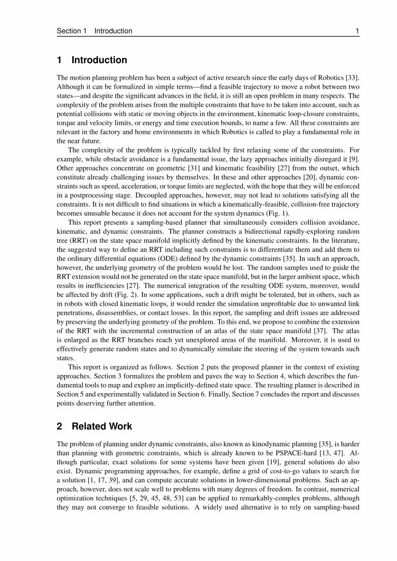
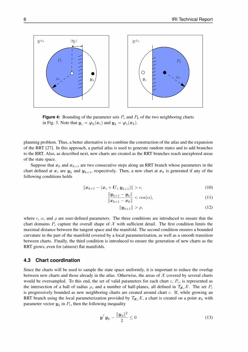

Acknowledgements
This research has been partially funded by project DPI2014-57220-C2-2-P
IRI reports
This report is in the series of IRI technical reportsAll IRI technical reports are available for download at the IRI websitehttpwwwiriupcedu


