1 / 15 28. Oktober 2008 KISSsoft Tutorial: Modeling a Shaft __________________________________________________________________________________________ For release 10/2008 kisssoft-tut-006-E-shaft-editor.doc Last modification 10/28/2008 5:14:00 PM __________________________________________________________________________________________ 1 Starting the Shaft Editor 1.1 General Remarks This tutorial is an introductory guide to how to model a shaft with the use of the Shaft calculation module. For a detailed description of the calculation features, see Tutorial 005: Shaft Analysis and Tutorial 007: Roller Bearings. All tutorials are available at http://www.kisssoft.ch/english/downloads/index.php. 1.2 Starting KISSsoft Step 1: After having installed and released KISSsoft as test or commercial version (see installation instructions), start KISSsoft by clicking Start > Programs > KISSsoft 10-2008 in the Windows task bar. The KISSsoft start window opens. Step 2: Start the shaft calculation module by double-clicking the item Shaft calculation [W010]in the Modules tree window, as depicted in Fig. 1.2-1. The Shaft calculation main window opens (see Fig. 1.2-2). KISSsoft Tutorial 006: Modeling a Shaft
Transcript
1 / 15 28. Oktober 2008
KISSsoft Tutorial: Modeling a Shaft
__________________________________________________________________________________________ For release 10/2008
kisssoft-tut-006-E-shaft-editor.doc Last modification 10/28/2008 5:14:00 PM __________________________________________________________________________________________
1 Starting the Shaft Editor
1.1 General Remarks
This tutorial is an introductory guide to how to model a shaft with the use of the Shaft calculation module. For a detailed description of the calculation features, see Tutorial 005: Shaft Analysis and Tutorial 007: Roller Bearings. All tutorials are available at http://www.kisssoft.ch/english/downloads/index.php.
1.2 Starting KISSsoft
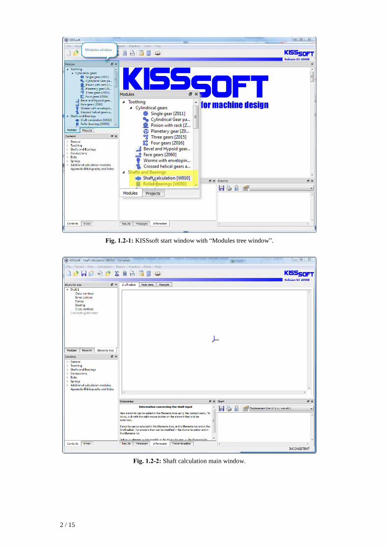
Step 1: After having installed and released KISSsoft as test or commercial version (see installation instructions), start KISSsoft by clicking Start > Programs > KISSsoft 10-2008 in the Windows task bar. The KISSsoft start window opens. Step 2: Start the shaft calculation module by double-clicking the item �Shaft calculation [W010]� in the �Modules tree window�, as depicted in Fig. 1.2-1. The Shaft calculation main window opens (see Fig. 1.2-2).
Fig. 1.2-1: KISSsoft start window with �Modules tree window�.
Fig. 1.2-2: Shaft calculation main window.
3 / 15
1.3 Example Problem
The shaft with the properties as depicted in Fig. 1.3-1 is to be modelled (blue faces: loads, yellow faces: bearings).
Fig. 1.3-1: Example shaft.
Shaft elements: 1 Notch effect due to interference fit 2 Keyway 3 Line load 4 Keyway 5 Radius 6 Coupling (source of power) 7 Radius 8 Radial bore 9 Radius 10 Cylindrical gear (drain of power) 11 Longitudinal bore
4 / 15
2 Modeling the Shaft Geometry
2.1 Coordinate System
Fig. 2.1-1: Shaft coordinate system (right-hand rule applies).
y=0: Left end of shaft. Positive x-axis: Points out of the screen Positive y-axis: From left to right, in direction of shaft axis Positive z-axis: From bottom to top Pos. of application: Angle between positive x-axis and towards positive z-axis. Counter-
clockwise positive.
2.2 Editing Views
The following editing functions are available in the Shaft editor: Function Explanation
�+�/�-�/�Home� Zoom in, zoom out, centre graphic Left mouse button Select element Right mouse button Open context menu: zoom in, zoom out, centre graphic Delete Delete selected element
2.3 Entering Shaft Sections
Modeling a shaft in KISSsoft requires information on the main geometry, the notches, loads and supports/bearings. As elements of the shaft, first the so-called main elements (e.g. cylinders), followed by the sub elements (e.g. notches), loads (e.g. forces and momentums) and supports/bearings have to be defined. Fig. 2.3-1 shows an overview of the �Elements-tree� structure and Table 2.3-1 comprises information on elements in group level of the Elements-tree. The Connecting elements entry allows two shafts to be interconnected. See Tutorial m: Modeling multiple shafts for a detailed description of how to model systems of shafts.
5 / 15
Fig. 2.3-1: �Elements-tree� and element hierarchy.
Table 2.3-1: Group level elements in the �Elements-tree�.
Element Information
on Required input Determination of
Outer/
Inner
contour
shaft section diameter, length of shaft section, surface, type and geometry of notches as sub elements
A, Ixx, Izz, Ip, Wxx, Wzz, Wp, k
Forces external loads centric or ex-centric force/momentum vectors, machine elements (like gears) for load introduction, additional masses
Fy, Qx, Qz, Mbx, Mbz, T
Bearing supports, roller bearings
Selection of roller bearings, information on bearing stiffness, degrees of freedom
reaction forces, boundary conditions
Cross
sections
critical cross section
effect of notch, position, geometry, surface roughness
notch factor, strain
2.3.1 External Contour
The shaft is modelled as a series of cones/cylinders. Right-click the Outer contour item in the �Elements-tree� window and choose the �Cylinder� element from the list. Define the length (l=80mm) and diameter (d=40mm) of the first cylindrical section in the �Element editor window�. Also, define surface roughness to be Rz=8.0. Repeat these steps for all cylindrical sections knowing that every new cylindrical element is appended to the right (positive y-direction) of the preceding one.
6 / 15
Fig. 2.3-2: Definition of first cylindrical element.
Fig. 2.3-3: Parameterizing the cylindrical element.
Repeat these steps for the three remaining sections, using the dimensions shown in the table below: Section No. Length [mm] Diameter [mm] Surface quality [-]
2 40 55 N7 3 80 50 N7 4 35 35 N7 The model should now look like as shown below. Right-click to open the context menu: Choose �Fit window� to resize the drawing according to window frame.
7 / 15
Fig. 2.3-4: Shaft model after adding the external contours.
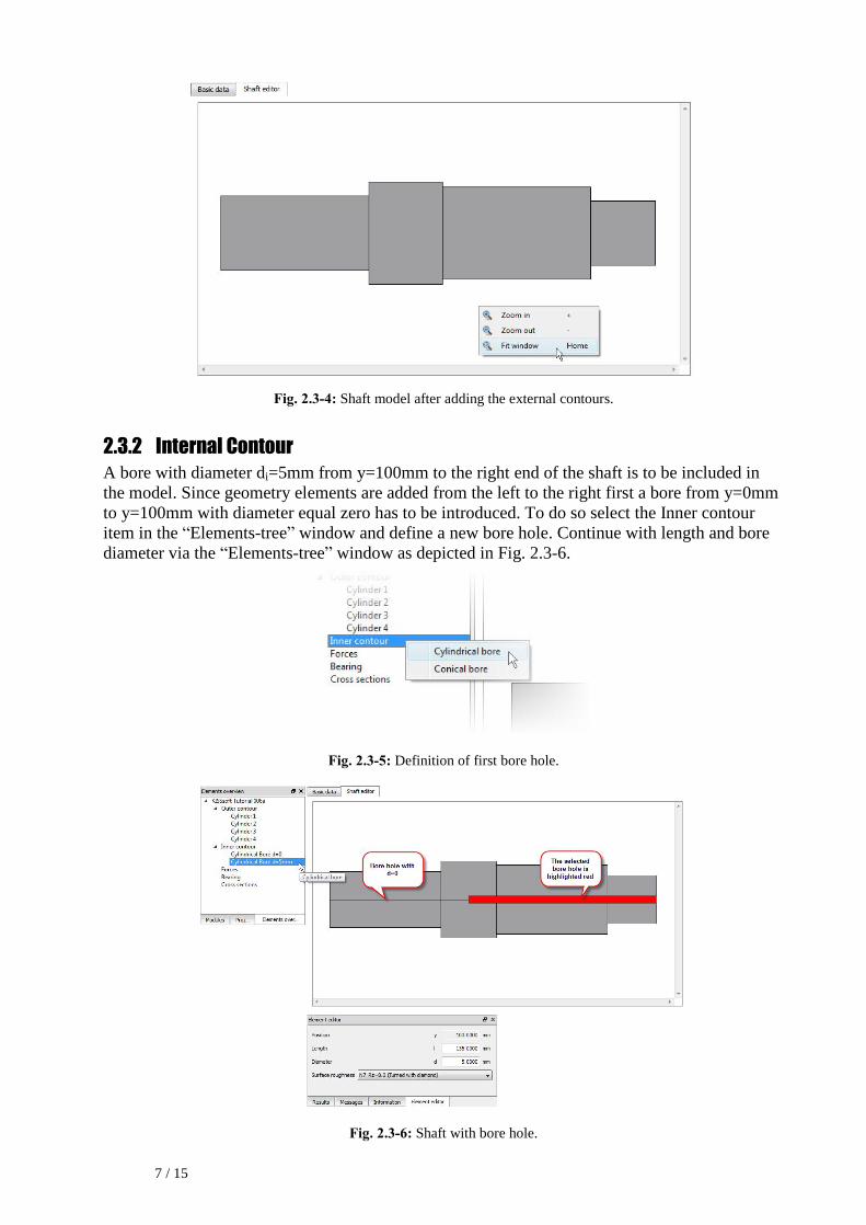
2.3.2 Internal Contour
A bore with diameter di=5mm from y=100mm to the right end of the shaft is to be included in the model. Since geometry elements are added from the left to the right first a bore from y=0mm to y=100mm with diameter equal zero has to be introduced. To do so select the Inner contour item in the �Elements-tree� window and define a new bore hole. Continue with length and bore diameter via the �Elements-tree� window as depicted in Fig. 2.3-6.
Fig. 2.3-5: Definition of first bore hole.
Fig. 2.3-6: Shaft with bore hole.
8 / 15
2.4 Defining Notches
Introduce a notch to a shaft section by right-clicking the respective main element (e.g. Cylinder 1, see Fig. 2.4-1) in the �Elements-tree� and choose the desired notch effect from the context menu. Parameterize the notch in the �Elements-editor�.
2.4.1 Entering Radii
Radii are present on the right end of the first shaft section and on the left end of the third and fourth section. In order to define the radius on the right side of the first shaft section right-click the first element in the list of �Outer Contour� elements and choose �Radius right� from the list. Use the �Elements-tree� window to enter the radius of the newly introduced element (see Fig. 2.4-1):
Fig. 2.4-1: Steps for adding a radius.
This procedure is now repeated for the two remaining radii. For the second radius, the third shaft section is to be selected and a radius on the left with r=1mm is to be added. For the third radius, the fourth section is to be selected and a radius on the left with r=4mm is added. The model should now look as follows:
Fig. 2.4-2: Shaft model after adding the radii.
9 / 15
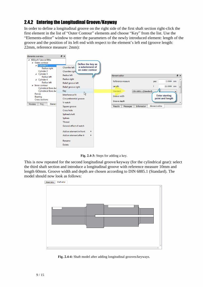
2.4.2 Entering the Longitudinal Groove/Keyway
In order to define a longitudinal groove on the right side of the first shaft section right-click the first element in the list of �Outer Contour� elements and choose �Key� from the list. Use the �Elements-editor� window to enter the parameters of the newly introduced element: length of the groove and the position of its left end with respect to the element�s left end (groove length: 22mm, reference measure: 2mm):
Fig. 2.4-3: Steps for adding a key.
This is now repeated for the second longitudinal groove/keyway (for the cylindrical gear): select the third shaft section and introduce a longitudinal groove with reference measure 10mm and length 60mm. Groove width and depth are chosen according to DIN 6885.1 (Standard). The model should now look as follows:
Fig. 2.4-4: Shaft model after adding longitudinal grooves/keyways.
10 / 15
2.4.3 Introducing the Interference Fit
The coupling on the left end of the shaft uses not only a key but also an interference fit to introduce the torque. This interference fit will result in a notch effect as well. Add the interference fit element by right-clicking on the first �Outer contour� element and select �Interference fit� from the list. Now, define the position of the left end of the interference fit (pos=0mm), the length (l=40mm) and choose the type of interference from the drop-down list in the �Elements-editor� window.
Fig. 2.4-5: �Elements-editor� for the interference fit.
2.4.4 Adding the Radial Bore
In the middle of the second shaft section a radial bore has to be applied (e.g. for lubrication purposes). Model this element by right-clicking the second element in the �Outer contour� tree and choose �Cross hole� from the list. The �Elements-editor� enables you to set the parameters to Diameter d=5mm and �Reference measure� pos=20mm.
Fig. 2.4-6: Element editor for the radial bore (cross hole).
The model should now look as follows:
11 / 15
Fig. 2.4-7: Shaft model after adding the interference fit and radial bore.
2.4.5 Introducing Loads
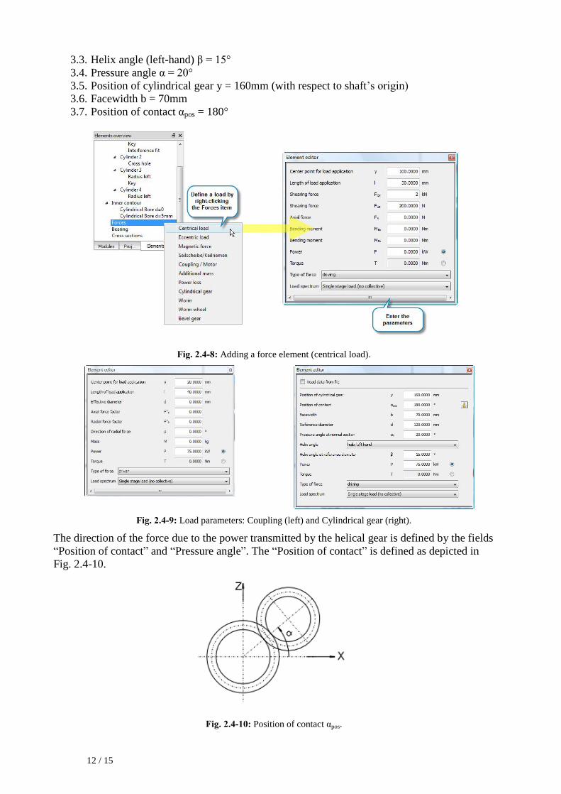
In this step the external forces acting on the shaft are modelled. Basically, any load is applied by right-clicking the �Forces� element in the �Elements-tree window�. A �Centrical load/Eccentric� load is determined by its position and three components, one per Cartesian axis. This force vector can either act through the centre line of the shaft or with an offset. Note that in the �Shafts editor� a load vector is represented by an arrow always pointing in negative z-direction. Besides the definition of forces as a general force/moment vector, KISSsoft provides the possibility to define external loads using machine elements. The resulting forces acting on the shaft are then automatically calculated based on the geometry of the machine element, its function and power rating (see Fig. 2.4-9). The shaft is driven by a coupling on its left end. The shaft drives an external application with the helical gear according to a power of 75kW. In the middle of the shaft a line-load is added. The speed of the shaft is defined in the tab �Basic data� of the shaft analysis module, not in the tab �Shaft editor�. Add a load by right-clicking on the �Forces� item in the �Elements-tree window�. The following load elements are to be introduced to the overall shaft model: 1. Coupling/Motor
1.1. Power P = 75kW (driven) 1.2. Length of load application l = 40mm 1.3. Center point for load application y = 20mm (with respect to shaft�s origin)
2. Centrical load
2.1. Shearing force in x-direction Fx = 2kN 2.2. Shearing force in z-direction Fz = 200N 2.3. Length of load application l = 30mm 2.4. Center point for load application y = 100mm (with respect to shaft�s origin)
3. Cylindrical gear
3.1. Power P = 75kW (driving) 3.2. Reference diameter d = 120mm
12 / 15
3.3. Helix angle (left-hand) â = 15° 3.4. Pressure angle á = 20° 3.5. Position of cylindrical gear y = 160mm (with respect to shaft�s origin) 3.6. Facewidth b = 70mm 3.7. Position of contact ápos = 180°
Fig. 2.4-8: Adding a force element (centrical load).
Fig. 2.4-9: Load parameters: Coupling (left) and Cylindrical gear (right).
The direction of the force due to the power transmitted by the helical gear is defined by the fields �Position of contact� and �Pressure angle�. The �Position of contact� is defined as depicted in Fig. 2.4-10.
Fig. 2.4-10: Position of contact ápos.
13 / 15
Note that angle ápos is counted positive counter-clockwise with respect to the y-axis.
If the overall torque is unbalanced a message comes up telling that the sum of torques is not zero. Since a shaft�s stationary operating point requires the accelerating loads to be null you have to check the applied torques. Most probably one or more errors in the definition of the Direction parameters occurred. A definition of the Direction parameter is given in Table 2.4-1.
Table 2.4-1: Definition of Direction.
The shaft is � driving. driven. Power flows � out of into � the shaft. Torque turns in � opposite same � direction of
shaft�s rotation. After adding the force elements, the model should look as follows:
Fig. 2.4-11: Shaft model after adding the load elements.
2.4.6 Adding the Bearings
The two bearings are added by selecting the item �Bearing� in the �Elements-tree window�. You can choose between �Bearing (in general)� and �Roller bearing�. General bearings allow for the definition of degrees of freedom where roller bearings incorporate constraints based on their mechanical properties (e.g. additional axial forces). The y-position (centre of the bearing), the type, size (internal diameter) and name of the bearing have to be defined in the �Elements-editor� window. Furthermore, it has to be defined whether the bearing will take axial forces and from which side. Choosing the option �Roller bearing stiffness calculated from inner geometry� from the dropdown-list Roller bearing in tab �Basic data� introduces translational/rotational stiffness to the respective bearing based on parameters of its inner geometry (diameter of rollers, radii of raceways, �). If no such data is given the parameters will be approximated based on the bearing�s type and size. See also section 2.6.1. Line supports have to be modelled using a number of separate supports. See Tutorial 007: Roller bearings on bearing analysis.
14 / 15
The following load elements are to be introduced to the overall shaft model: 1. Bearing (SKF *6208)
1.1. Position y = 65mm (with respect to shaft�s origin) 1.2. Type of bearing: Fixed bearing adjusted on the left side 1.3. Type: Deep groove ball bearing (single row) 1.4. Inside diameter d = 40mm
2. Bearing (SKF *6207)
2.1. Position y = 216mm (with respect to shaft�s origin) 2.2. Type of bearing: Fixed bearing adjusted on the right side 2.3. Type: Deep groove ball bearing (single row) 2.4. Inside diameter d = 35mm
Fig. 2.4-12: Adding a roller bearing (left bearing).
After adding the bearings, the model should look like as follows:
Fig. 2.4-13: Shaft model upon adding the bearing elements.
2.5 Cross Sections
KISSsoft provides two definitions of sections for strength calculations: the �Limited cross section� and the �Free cross section�. While for a �Limited cross section� the calculation module returns the actual notch factors for the given y-coordinate it is up to the user�s demands to alter these parameters arbitrarily for the �Free cross section�. For a detailed description of strength calculation see Tutorial 005: Shaft Analysis.
15 / 15
2.6 Notes
2.6.1 Bearing calculation
Choose your desired bearing calculation via the drop-down list �Roller bearing� in the �Basic data� input window (see Fig. 2.6-1).
There are three different bearing calculations available:
1. Classical calculation with or w/o consideration of pressure angle These two options comprise the features well-known from KISSsoft Rel. 04/06: Bearings are considered constraints for displacement and rotation with optional offset, adjustment, stiffness and clearance.
2. Calculation of the stiffness based on inner geometry This method evaluates service life like in the classical roller calculation but with respect to roller geometry, number of rollers, radii of raceways, etc. The bearing�s stiffness and
offset are computed based on nonlinear material laws.
3. Calculation according to DIN/ISO 281 Annex 4 The guideline DIN ISO 281-4:2003 Dynamic load ratings and rating life covers modified service life calculations with respect to the bearing�s inner geometry. Also, stiffness and offset are computed based on nonlinear material laws.
2.6.2 Shaft systems
The calculation module �Shaft systems� allowed modeling and calculation from different shafts in one calculation model. These kind of modeling is useful e.g. for calculation the shaft in planetary gear.