116
Notes on Stochastic Processes Kiyoshi Igusa December 17, 2006

Notes on Stochastic Processes
Kiyoshi Igusa
December 17, 2006

ii
These are lecture notes from a an undergraduate course given at Brandeis University in Fall 2006using the second edition of Gregory Lawler’s book “Introduction to Stochastic Processes”.

Contents
Syllabus
0. Linear equations
(a) linear differential equations in one variable
(b) Kermack-McKendrick epidemic model
(c) first order equations
(d) linear difference equations
1. Finite Markov chains
(a) definitions
(b) communication classes
(c) classification of states: transient and recurrent
(d) periodic chains
(e) invariant distributions
(f) return time
(g) substochastic matrix
(h) Leontief model
2. Countable Markov chains
(a) extinction probability
(b) random walk
(c) Stirling’s formula
3. Continuous Markov chains
(a) making time continuous
(b) Poisson to Markov
(c) definition of continous Markov chain
(d) probability distribution vector
iii

iv CONTENTS
(e) equilibrium distribution and positive recurrence
(f) birth-death chain
4. Optimal stopping time
(a) basic problem
(b) basic solutions
(c) cost function
(d) discount payoff
5. Martingales
(a) intuitive description
(b) conditional expectation
(c) σ-filtration
(d) optimal sampling theorem
(e) martingale convergence theorem
6. Renewal
(a) renewal theorem
(b) age of current process
(c) M/G/1-queueing
7. (Time) Reversal
(a) basic equation
(b) reversible process
(c) symmetric process
(d) statistical mechanics
8. Brownian motion
(a) definition
(b) martingales and Levy’s theorem
(c) reflection principle
(d) fractal dimension of Z
(e) heat equation
(f) recurrence and transience
(g) fractal dimension of path
(h) drift

CONTENTS v
9. Stochastic integration
(a) idea
(b) discrete integration
(c) integration with respect to Brownian motion
(d) Ito’s formula
(e) continuous martingales
(f) Feynman-Kac
(g) Black-Scholes
References

Math 56a: Introduction to Stochastic Processes and Models
Kiyoshi Igusa, Mathematics
August 31, 2006
A stochastic process is a random process which evolves with time. The basic model is the Markovchain. This is a set of “states” together with transition probabilities from one state to another.For example, in simple epidemic models there are only two states: S = “susceptible” and I =“infected.” The probability of going from S to I increases with the size of I. In the simplestmodel The S → I probability is proportional to I, the I → S probability is constant and time isdiscrete (for example, events happen only once per day). In the corresponding deterministic modelwe would have a first order recursion.
In a continuous time Markov chain, transition events can occur at any time with a certain prob-ability density. The corresponding deterministic model is a first order differential equation. Thisincludes the “general stochastic epidemic.”
The number of states in a Markov chain is either finite or countably infinite. When the collectionof states becomes a continuum, e.g., the price of a stock option, we no longer have a “Markovchain.” We have a more general stochastic process. Under very general conditions we obtain aWiener process, also known as Brownian motion. The mathematics of hedging implies that stockoptions should be priced as if they are exactly given by this process. Ito’s formula explains how tocalculate (or try to calculate) stochastic integrals which give the long term expected values for aWiener process.
This course will be a theoretical mathematics course. The goal is to give rigorous mathematicaldefinitions and derive the consequences of simple stochastic models, most of which will be Markovchains. I will not explain the principles of biology, economics and physics behind the models,although I would invite more qualified guest lecturers to explain the background for the models.There will be many examples, not just the ones outlined above.
The prerequisite for the course will be Math 36a (probability using calculus), linear algebra (Math15) and multivariable calculus (Math 20). Basic linear differential equations will be reviewed at thebeginning of the course. Probability will not be reviewed. This is an advanced course for studentsalready familiar with probability. Linear algebra is also heavily used. Statistics is not required.
1

Outline of course
1. Review of linear recursion and linear differential equations.
2. Definitions and general notions about stochastic processes
3. Finite Markov chains
4. Renewal processes
5. Continuous time Markov chains
6. Martingales
7. Wiener processes (Brownian motion)
8. Stochastic integration and Ito’s formula
9. Applications to population biology and epidemiology
10. Application to financial security analysis
Applications will vary according to the interests of students and teacher.
Required text Introduction to Stochastic Processes, Gregory Lawler, Chapman & Hall
Recommended books:
• Markov Chains, J.R. Norris, Cambridge University Press. (This is an excellent book whichdevelops Markov chains in a more leisurely way but does not have stochastic integrals.)
• Epidemic Modelling, An Introduction, D.J. Daley & J.Gani, Cambridge University Press
• Financial Derivatives, Pricing, Applications and Mathematics, Jamil Baz & George Chacko,Cambridge University Press
• The Mathematics of Financial Derivatives, A Student Introduction, Paul Wilmott, Sam How-ison, Jeff Dewynne, Cambridge University Press
Grading 50% homework, 50% in-class performance. Expected grade: A-/B+
There will be weekly homework. The first HW might have the problem: Find a formula for then-th Fibonacci number by solving the linear recurrence. Students are encouraged to work ontheir homework in groups and to access all forms of aid including expert advice, internet andother resources. The work you hand in should, however, be in your own words and in your ownhandwriting. And you should understand what you have written.
In-class activities: “quizzes” will be given every week or other week. Students should form groupsof 3 or 4 to work on these problems in class, solve them and help other students in the group to
2

understand them. Each group should hand in their answers signed by all members of the group.Every student is required to give at least one short oral presentation in front of the class. Attendanceis required and counts as part of the grade.
Students with disability If you are a student with a documented disability at Brandeis Universityand if you wish to request a reasonable accommodation for this class, please see the instructorimmediately.
Academic integrity All members of the Brandeis academic community are expected to main-tain the highest standard of academic integrity as outlined in “Rights and Responsibilities.” Anyviolations will be treated seriously.
3

MATH 56A: STOCHASTIC PROCESSESCHAPTER 0
0. Chapter 0
I “reviewed” basic properties of linear differential equations in onevariable. I still need to do the theory for several variables.
0.1. linear differential equations in one variable. In the first lec-ture I discussed linear differential equations in one variable. The prob-lem in degree n = 2 is to find a function y = f(x) so that:
(0.1) y′′ + ay′ + by + c = 0
where a, b, c are constants.The general n-th order linear diff eq in one variable is:
y(n) + a1y(n−1) + a2y
(n−2) + · · ·+ any + an+1 = 0
where a1, · · · , an+1 are constant.
0.1.1. associated homogeneous equation. The standard procedure is tofirst take the associated homogeneous equation which is given by settingan+1 = 0. For the 2nd order equation we get:
(0.2) y′′ + ay′ + by = 0
Lemma 0.1. If y = f(x) is a solution of the homogeneous equationthen so is y = αf(x) for any scalar α.
Lemma 0.2. If y = f0(x) is a solution of the original equation (0.1)and y = f1(x) is a solution of the homogeneous equation (0.2) theny = f0(x)+f1(x) is a solution of the original equation (0.1). Similarly,if f0, f1 are solutions of the homogeneous equation then so is f0 + f1.
Theorem 0.3. The set of solutions of the homogenous equation is avector space of dimension equal to n (the order of the equation).
This means that if we can find n linearly independent solutionsf1, f2, · · · , fn of the homogeneous equation then the general solution(of the homogenous equation) is a linear combination:
y = α1f1 + α2f2 + · · ·+ αnfn
Date: September 28, 2006.1
2 MATH 56A: STOCHASTIC PROCESSES CHAPTER 0
0.1.2. complete solution of linear diffeqs. A general solution of the lin-ear diffeq is given by adding a particular solution f0 to the generalsolution of the homogeneous equation:
y = f0 + α1f1 + α2f2 + · · ·+ αnfn
The particular solution is easy to find:
f0(x) = −an+1
an
if an 6= 0
f0(x) = −− an+1
an−1
x
if an = 0 but an−1 6= 0.The solutions of the homogeneous equations are given by guessing.
We just need to find n linearly independent solutions. We guess thaty = eλx. Then
yk = λkeλx
So, the homogenous equation is:
λneλx + a1λn−1eλx + · · ·+ ane
λx = 0
Since eλx is never zero we can divide to get:
λn + a1λn−1 + · · ·+ an = 0
This is a monic (coefficient of λn is 1) polynomial of degree n. So, ithas n complex roots λ1, λ2, · · · , λn. If the roots are distinct then thesolutions
f1(x) = eλ1x, f2(x) = eλ2x, · · ·are linearly independent and span the solution space.
If roots repeat, e.g., if λ1 = λ2 = λ3 then the functions f2, f3 aregiven by
f2(x) = xeλ1x, f3(x) = x2eλ1x,
0.1.3. separation of variables. Finally, I talked about separation of vari-ables. This just means put all the x’s on one side of the equation andall the y’s on the other side. For example:
dy
dx= xy
This is a nonlinear diffeq. Separating variables we get:
dy
y= xdx

MATH 56A: STOCHASTIC PROCESSES CHAPTER 0 3
Now integrate both sides: ∫dy
y=
∫x dx
ln y =x2
2+ C
Note that there is only one constant. (You get a constant on both sidesand C is the difference between the two constants.) The final solutionis:
y = y0exp
(x2
2
)where y0 = eC .
0.2. Kermack-McKendrick. This is from the book Epidemic Mod-elling, An Introduction, D.J. Daley & J.Gani, Cambridge UniversityPress. Kermack-McKendrick is the most common model for the gen-eral epidemic. I made two simplifying assumptions:
• the population is homogeneous and• no births or deaths by other means
Since there are no births, the size of the population N is fixed.In this model there are three states:
S: = susceptibleI: = infectedR: = removed (immune)
Let x = #S, y = #I, z = #R. So
N = x + y + z
I assume that z0 = 0 (If there are any “removed” people at t = 0 weignore them.)
As time passes, susceptible people become infected and infected re-cover and become immune. So the size of S decreases and the size ofR increases. People move as shown by the arrows:
S −→ I −→ R
The infection rate is given by the Law of mass action which says:
The rate of interaction between two different subsets of the populationis proportional to the product of the number of elements in each subset.
So,dx
dt= −βxy
where β is a positive constant.

4 MATH 56A: STOCHASTIC PROCESSES CHAPTER 0
Infected people recover at a constant rate:
dz
dt= γy
where γ is a positive constant.This is a system of nonlinear equations. To solve it we make it linear
by dividing:dx
dz=
dx/dt
dz/dt=−βxy
γy=−βx
γThis is a linear differential equation with solution
x = x0exp
(−β
γz
)= x0e
−z/ρ
where ρ = γ/β is the threshold population size.Since x + y + z is fixed we can find y:
y = N − x− z = N − x0e−z/ρ − z
Differentiating gives:dy
dz=
x0
ρe−z/ρ − 1
d2y
dz2= −x0
ρ2e−z/ρ < 0
So, the function is concave down with initial slope
dy
dz=
x0
ρ− 1
which is positive if and only if x0 > ρ. So, according to this model, thenumber of infected will initially increase if and only if the number ofsusceptibles is greater than the threshold value ρ = γ/β.
By plotting the graphs of the functions we also see that the infectionwill taper off with a certain number of susceptibles x∞ who never getinfected.

MATH 56A: STOCHASTIC PROCESSES CHAPTER 0 5
0.3. systems of first order equations. I explained that differentialequations involving second and higher order derivatives can be reducedto a system of first order equations by introducing more variables. ThenI did the following example.
y′ = z
z′ = 6y − z
In matrix form this is:
d
dt
(yz
)=
(0 16 −1
)(yz
)Which we can write as Y = AY with
Y =
(yz
), A =
(0 16 −1
)0.3.1. exponential of a matrix. The solution of this equations is
Y = etAY0
where Y0 =
(y0
z0
)and
etA := I2 + tA +t2A2
2+
t3A3
3!+ · · ·
This works because the derivative of each term is A times the previousterm:
d
dt
tkAk
k!=
ktk−1Ak
k!=
tk−1Ak
(k − 1)!= A
tk−1Ak−1
(k − 1)!
So,d
dtetA = AetA
0.3.2. diagonalization (corrected). Then I explained how to computertA. You have to diagonalize A. This means
A = QDQ−1
where D is a diagonal matrix D =
(d1 00 d2
).
I should have explained this formula so that I get it right: If X1, X2
are eigenvalues of A with eigenvalues d1, d2 then AX1 = X1d1, AX2 =X2d2 and
A(X1X2) = (X1d1X2d2) = (X1X2)
(d1 00 d2
)

6 MATH 56A: STOCHASTIC PROCESSES CHAPTER 0
Solve for A gives
A = (X1X2)
(d1 00 d2
)(X1X2)
−1 = QDQ−1
where Q = (X1, X2).This is a good idea because A2 = QDQ−1QDQ−1 = QD2Q−1 and
more generally, tkAk = tkQDkQ−1. Divide by k! and sum over k toget:
etA = QetDQ−1 = Q
(etd1 00 etd2
)Q−1
0.3.3. eigenvectors and eigenvalues. The diagonal entries d1, d2 are theeigenvalues of the matrix A and Q = (X1X2) where Xi is the eigenvec-tor corresponding to di. This works if the eigenvalues of A are distinct.The eigenvalues are defined to be the solutions of the equation
det(A− λI) = 0
but there is a trick to use for 2 × 2 matrices. The determinant of amatrix is always the product of its eigenvalues:
det A = d1d2 = −6
The trace (sum of diagonal entries) is equal to the sum of the eigenval-ues:
trA = d1 + d2 = −1
So, d1 = 2, d2 = −3. The eigenvalues are X1 =
(12
)and X2 =
(1−3
).
So
Q = (X1X2) =
(1 12 −3
)Q−1 =
1
det Q
(−3 −1−2 1
)=
(3/5 1/52/5 −1/5
)The solution to the original equation is(
yz
)=
(1 12 −3
)(e2t 00 e−3t
)(3/5 1/52/5 −1/5
)(y0
z0
)

MATH 56A: STOCHASTIC PROCESSES CHAPTER 0 7
0.4. Linear difference equations. We are looking for a sequenceof numbers f(n) where n ranges over all the integers from K to N(K ≤ n ≤ N) so that
(0.3) f(n) = af(n− 1) + bf(n + 1)
I pointed out that the solution set is a vector space of dimension 2.So we just have to find two linearly independent solutions. Then Ifollowed the book.
The solution has the form f(n) = cn where you have to solve for c:
cn = acn−1 + bcn+1
(0.4) bc2 − c + a = 0
c =1±
√1− 4ab
2bThere were two cases.
Case 1: (4ab 6= 1) When the quadratic equation (0.4) has two rootsC1, c2 then the linear combinations of cn
1 and cn2 give all the solutions
of the homogeneous linear recursion (0.3).Case 2: (4ab = 1) In this case there is only one root c = 1
2band the
two independent solutions are f(n) = cn and ncn. The reason we geta factor of n is because when a linear equation has a double root thenthis root will also be a root of the derivative. This gives f(n) = ncn−1
as a solution. But then you can multiply by the constant c since theequation is homogeneous.
Example 0.4. (Fibonacci numbers) These are given by f(0) = 1, f(1) =1 and f(n + 1) = f(n) + f(n− 1) or:
f(n) = f(n + 1)− f(n− 1)
This is a = −1, b = 1. The roots of the quadratic equation are c = 1±√
52
.So,
f(n) =1√5
(1 +
√5
2
)n
− 1√5
(1−
√5
2
)n
This is a rational number since it is Galois invariant (does not changeif you switch the sign of
√5). However, it is not clear from the formula
why it is an integer.

MATH 56A: STOCHASTIC PROCESSESCHAPTER 1
1. Finite Markov chains
For the sake of completeness of these notes I decided to write asummary of the basic concepts of finite Markov chains. The topics inthis chapter are:
(1) definition of a Markov chain(2) communication classes(3) classification of states(4) periodic/aperiodic(5) invariant probability distribution(6) return time(7) substochastic matrix
1.1. definition. A stochastic process is a random process which evolveswith time. In other words, we have random variables Xt, Yt, etc. whichdepend on time t. For example Xt could be your location at time t(where t is in the future).
A finite Markov chain is a special kind of stochastic process with thefollowing properties
• There are only a finite number of states. If we are talkingabout your location, this means we are only interested in whichbuilding you are in and not your exact position in the building.
• Time is discrete: For example, things change only at 1pm, 2pm,etc. and never at 1:12pm or any time in between. Xn is thestate at time n where n = 0, 1, 2, etc.
• No memory. Your (random) movement at time n depends onlyon Xn and is independent of Xt for t < n (You forget the pastand your decision making process is based only on the presentstate.)
• Time homogeneous: Your rules of movement are the same atall times.
To summarize: You have a finite number of building that you canmove around in. You can only move on the hour. Your decision makingprocess is random and depends only on your present location and not
Date: December 15, 2006.1

2 MATH 56A: STOCHASTIC PROCESSES CHAPTER 1
on past locations and does not take into account what time it is. (Youmove at midnight in the same way that you do at noon.)
Definition 1.1. A finite Markov chain is a sequence of random vari-ables X0, X1, · · · which take values in a finite set S called the statespace and for any n and any values of x0, x1, · · · , xn we have:
P(Xn+1 = x |X0 = x0, X1 = x1, · · · , Xn = xn) = P(X1 = x |X0 = xn)
The S × S matrix P with entries
p(x, y) := P(X1 = y |X0 = x)
is called the transition matrix.
For example, suppose that you have 4 points: 0,1,2,3 and at eachstep you either increase one or decrease one with equal probabilityexcept at the end points. Suppose that, when you reach 0, you cannotleave. (0 is called an absorbing state.) Suppose that when you reach 3you always go to 2. (3 is called a reflecting wall.) Then the transitionmatrix is
P =
1 0 0 0
1/2 0 1/2 00 1/2 0 1/20 0 1 0
Notice that the numbers are all nonnegative and the numbers in eachrow add up to 1. This characterizes all transition matrices.
In the discussion of Markov chains, there are qualitative non-numericalconcepts and quantitative, computational concepts. The qualitativeconcepts are: communication classes, their classification and periodic-ity.
1.2. communication classes. Two states communicate with each otherif they are equal or if it is possible (with positive probability) to getfrom either one to the other in a finite amount of time. We write x ↔ y.This is an equivalence relation and the equivalence classes are calledcommunication classes.
In the example above, 0 and 1, 2, 3 are the communication classes.A Markov chain is irreducible if it has only one communication class,
i.e., if it is possible to get from any state to any other state.
1.3. classification of states: transient and recurrent. There aretwo types of communication classes: recurrent and transient. At thispoint, I allowed the state space S to be infinite so that you don’t getthe wrong idea.

MATH 56A: STOCHASTIC PROCESSES CHAPTER 1 3
A communication class C is recurrent if for any state x ∈ C, youwill keep returning to x an infinite number of times with probabilityone. A communication class C is transient if, starting at any x ∈ C,you will return to x only a finite number of times with probability one.
The theorem is that these are the only two possibilities. I provedthis in class:
Lemma 1.2. If p = p(i, j) > 0 and i is recurrent then so is j. In fact,if you start in state i you will go to state j an infinite number of timeswith probability one.
Proof. This is the same as saying that the probability of going to statej only a finite number of times is zero. To prove this suppose that theMarkov chain goes to state j only a finite number of times. Then thereis a last time, say Xm = j. Then you can never return to j.
But i is recurrent. So, with probability one, you will go to i an infinitenumber of times after time m. Say at times n1 < n2 < n3 < · · · (all> m). But
P(Xn1+1 6= j |Xn1 = i) = 1− p
P(Xn2+1 6= j |Xn2 = i) = 1− p
The product is (1 − p)2, (1 − p)3, etc. which converges to 0. So, theprobability is zero that in all of these infinite times that you visit i youwill never go to j. This is what I was claiming.
Theorem 1.3. Once you leave a communication class you can neverreturn.
Theorem 1.4. Recurrent communication classes are absorbing.
The lemma shows that, if you could leave a recurrent communicationclass, you will with probability one. This would be a contradiction tothe definition of recurrent. So, you cannot leave a recurrent class.
The lemma that I proved can be rephrased as follows:
Lemma 1.5. If you make an infinite number of attempts and you havea fixed positive probability p of success then, with probability one, youwill succeed an infinite number of times.
The strong law of large numbers says that, with probability one,the proportion of trials which are successful will converge to p as thenumber of trials goes to infinity. I.e., the experimental value of theprobability p will converge to the theoretical value with probabilityone.

4 MATH 56A: STOCHASTIC PROCESSES CHAPTER 1
1.4. periodic chains. We are interested in the time it takes to returnto a state i. The return time Ti to state i is the smallest positive integern so that Xn = i given that X0 = i. In other words, you start at state iand count how many turns it takes to return to the same state i. Thisnumber is Ti. It is random. For example, in the random walk examplegiven above, P(T3 = 2) = 1/2, P(T2 = 2) = 3/4.
The period of a state i is the greatest common divisor of all possiblereturn times to state i. For the random walk on an infinite straightline (or on a finite line with reflecting walls), the period of every stateis 2 because it always takes an even number of steps (the same numberright as left) to get back to the same point.
A state i is aperiodic if the period is 1.
Theorem 1.6. States in the same communication class have the sameperiod.
1.5. Invariant probability distribution.
Definition 1.7. A probability distribution π is called invariant if
πP = π
Remember that a probability distribution is a vector with nonnegativecoordinates adding up to 1:
n∑i=1
π(i) = 1, π(i) ≥ 0
where n is the number of states. As an application of the Perron-Frobenius theorem we get:
Theorem 1.8. If the Markov chain is irreducible and aperiodic thenP n converges to a matrix in which every row is equal to the invariantdistribution π which is unique:
P∞ =
ππ· · ·π
If the Markov chain is periodic then P n depends on n modulo the
period d. However, the average value of P n will still converge:
Theorem 1.9. For any finite Markov chain the average value of P n
converges to a matrix in which every row is equal to the unique invariantdistribution π:
limn→∞
1
n
n∑k=1
P k =
π· · ·π

MATH 56A: STOCHASTIC PROCESSES CHAPTER 1 5
Proof. Let
Sn =1
n
n∑k=1
P k
Then each row of Sn adds to 1 and
SnP = Sn +1
n(P n+1 − P )
So, SnP ≈ Sn and S∞P = S∞. Since each row of S∞ adds to 1,each row is equal to the invariant distribution π (which is unique byPerron-Frobenius).
1.6. Return time. I explained in class the relation between the returntime Ti to state i and the value of the invariant distribution π(i):
E(Ti) =1
π(i)
Proof. Begin with the last theorem:
π(j) = limn→∞
1
n
n∑m=1
P(Xm = j)
Now use the fact that probability is the expected value of the indicatorfunction: P(A) = E(I(A)) and expected value is linear:
∑E = E
∑π(j) = lim
n→∞
1
nE
(n∑
m=1
I(Xm = j)
)This is the average expected number of visits to state j. If, in n steps,you visit a state k times then the average time from one visit to thenext is n/k and the average number of visits is k/n. So they are inverseto each other:
π(j) =k
n=
1
n/k=
1
E(Tj)
1.7. substochastic matrix. If there are both absorbing classes andtransient classes in the Markov chain then you get a substochasticmatrix Q which is the transient-to-transient transition matrix: Q =(p(x, y)) where we take x, y only from transient states. (Actually, youcan take any subset of the set of states.) Since this is only part of thetransition matrix P , the rows may not add up to 1. But we know thatthe entries are all nonnegative and the rows add up to at most 1.
Definition 1.10. A substochastic matrix is a square matrix Q whoseentries are all nonnegative with rows adding up to at most 1.

6 MATH 56A: STOCHASTIC PROCESSES CHAPTER 1
I used a model from economics to explain what was the point ofdoing this.
1.7.1. Leontief model. In this model we have r factories which producegoods. For every dollar worth of goods that factor i produces, it needsqij dollars worth of the output of factory j. In order to be profitableor to at least break even we need the production cost to be less thanor equal to one dollar:
qi1 + qi2 + · · ·+ qir ≤ 1
In other words, each row of the matrix Q = (qij) must add up to atmost 1. So, Q is a substochastic matrix.
To analyze how this works we follow the dollar. qij represents goodsgoing from j to i and it represents money going from i to j.
Now look at the total amount of money and what happens to it. Outof each dollar that factory i gets, it must give
∑qij to other factories.
What remains:1−
∑qij
is profit. Let’s say it puts this money in the bank. When we add thebank to the system we get a Markov chain with r + 1 states. Thetransition matrix is P = (p(i, j)) where
p(i, j) =
qij if i, j 6= 0
1−∑
k qik if i 6= 0, j = 0
0 if i = 0, j 6= 0
1 if i = j = 0
Note that this formula can be used to convert any substochastic matrixinto a Markov chain by adding one absorbing state.
Problem The problem is to figure out how much each factory needsto produce in order for the net production (not counting inter-industryconsumption) to be equal to a fixed vector γ. This is the consumptionvector. The consumer wants γi dollars worth of stuff from factory i.To find the answer we just follow the money after the consumer buysthe goods.
I explained it in class like this: The consumer orders γi worth ofgoods from factory i. On day zero, each factory i produces the re-quested goods using its inventory of supplies. Then it orders suppliesfrom the other factories to replenish its inventory. On day one, eachfactory produces goods to fill the orders from the other factories usingits inventory. And so on. Eventually, (in the limit as n → ∞), theinventories are all back to normal and all the money is in the bank as-suming that all the factories are transient states. The total production

MATH 56A: STOCHASTIC PROCESSES CHAPTER 1 7
is given by adding up the production on each day. Factory i producesγi on day 0, ∑
j
γjqji = (γQ)i
on day 1, ∑j
γjqjk
∑k
qki = (γQ2)i
on day 2, (γQ3)i on day 3, etc. So, the total production of factory i is
(γ(I + Q + Q2 + Q3 + · · · ))i = (γ(I −Q)−1)i
Lemma 1.11. The factories are all transient states if and only if I−Qis invertible.
Proof. If the factories are all transient then the money will all even-tually end up in the bank. Equivalently, the matrices Qn converge tozero. So I −Q is invertible. Conversely, if there is a recurrent class, itmust consist of nonprofit organizations which require only the outputfrom other nonprofits. Then these nonprofit factories give a Markovprocess with equilibrium distribution π. This will be a vector withπQ = π. So, it is a null vector of I − Q showing that I − Q is notinvertible.
1.7.2. avoiding states. Substochastic matrices are used to calculate theprobability of reaching one set of states A before reaching another setB (assuming that they are disjoint subsets of S). To do this you firstcombine them into two recurrent states. You also need to assumethere are no other recurrent states (otherwise the Markov chain couldget stuck in a third state and never reach A or B).
Suppose that there are n transient states and two absorbing statesA and B. Let Q be the n× n transient-to-transient transition matrixand let S be the n × 2 transient-to-recurrent matrix. Then the (i, A)entry of QkS is the probability of getting from state i to state A inexactly k + 1 steps. So, the total probability of ending up in state A is
Pi(A) = ((I + Q + Q2 + Q3 + · · · )S)iA = ((I −Q)−1S)iA

MATH 56A: STOCHASTIC PROCESSESCHAPTER 2
2. Countable Markov Chains
I started Chapter 2 which talks about Markov chains with a count-ably infinite number of states. I did my favorite example which is onpage 53 of the book.
2.1. Extinction probability. In this example we consider a popu-lation of one cell creatures which reproduce asexually. At each timeinterval, each creature produces X offspring and then dies. Here X is arandom variable equal to 0, 1, 2, 3 etc with probabilities pk = P(X = k).
You can read the complete analysis in the book, but what I explainedin class was the most striking part: if the average number of offspringis equal to 1 (and it is somewhat random, i.e., not always equal to 1)then the probability of extinction of the population is one.
In this model the state space is the set of nonnegative integers. Ifthe state is i then there are i creature in the population. At each timeinterval each of these creatures dies and produces a random numberof offspring. The state 0 is an absorbing state. We want to know theprobability that we eventually land in that state. We start with thedefinition:
a := P(Xn = 0 eventually|X0 = 1)
So, a is the probability that the species eventually becomes extinct ifit starts out with exactly one creature. The theorem is that a = 1.This implies that population dies out if we start with any number ofcreatures. The reason is that, because of asexual reproduction, thedescendants of each individual will not mix and so, assuming indepen-dence of the probabilities of extinction for each “family,” we get that
ak = P(Xn = 0 eventually|X0 = k)
The point is that, if a = 1 then ak = 1 for any k ≥ 0.To calculate a we look at what happens after one time interval.
a =∑
k
P(Xn = 0 eventually|X1 = k)P(X1 = k) =∑
k
akpk
Date: September 28, 2006.1
2 MATH 56A: STOCHASTIC PROCESSES CHAPTER 2
But this is the generating function for pk which is defined by
φ(s) := E(sX) =∑
k
skP(X = k) =∑
k
skpk
The extinction probability is equal to the generating function!!
a = φ(a)
The generating function has the property that φ(1) = 1. Here is theproof:
φ(1) =∑
k
1kpk =∑
k
pk = 1
The derivative of φ(s) is
(2.1) φ′(s) =∑
k
ksk−1pk
If we put s = 1 we get the expected value of X (the number of offspring)which we are assuming is equal to 1.
φ′(1) =∑
k
kpk = E(X) = 1
The second derivative is
φ′′(s) =∑k≥2
k(k − 1)sk−2pk > 0
This is greater than zero (for all s) if p2 > 0 or pk > 0 for some k ≥ 2.But, if X has average 1 and is not always equal to 1 then it must besometimes more and sometimes less than 1. So, there is a positiveprobability that X ≥ 2. So, φ′′(s) > 0.
Now, graph the function y = φ(s). Since φ(1) = 1 and φ′(1) = 1, thegraph goes through the point (1, 1) with slope 1. Since it is concaveup, it has to curve away from the line y = s on both sides of that point.So, the only solution to the equation a = φ(a) is a = 1.
For the general analysis we need the following lemma.
Lemma 2.1. a is the smallest nonnegative solution to the equationa = φ(a).
Proof. The eventual extinction probability is a limit of finite extinctionprobabilities:
a = limn→∞
an
where
an = P(Xn = 0|X0 = 1)

MATH 56A: STOCHASTIC PROCESSES CHAPTER 2 3
These finite extinction probabilities are calculated recursively as fol-lows:
an =∑
k
P(Xn = 0|X1 = k)P(X1 = k|X0 = 1)
=∑
k
P(Xn−1 = 0|X0 = k)P(X1 = k|X0 = 1) =∑
k
akn−1pk = φ(an−1)
Let a be the smallest nonnegative real number so that a = φ(a). Thenwe just have to show that an ≤ a for every n ≥ 0. This is true forn = 0 since
a0 = P(X0 = 0|X0 = 1) = 0 ≤ a
Suppose by induction that an−1 ≤ a. Then we have to show thatan ≤ a. But, if you look at the equation (2.1) you see that φ′(s) ≥ 0.So,
an = φ(an−1) ≤ φ(a) = a
Therefore, an ≤ a for all n ≥ 0. So, a ≤ a. So, a = a.
Theorem 2.2. If E(X) > 1 then the probability of extinction is lessthan 1. If E(X) ≤ 1 then the probability of extinction is one, except inthe case when the population is constant (i.e., when p1 = 1).
Proof. By the lemma, the extinction probability a is the first point ofintersection of the graph of y = φ(s) with the graph of y = s. But φ(s)goes through the point (1, 1) with slope E(X) and is always concaveup. A drawing of the graphs proves the theorem.

4 MATH 56A: STOCHASTIC PROCESSES CHAPTER 2
2.2. Random walk in an integer lattice. Today I want to explainthe proof that the simple random walk in the lattice Zd is recurrent ifd ≤ 2 and transient if d ≥ 3.
2.2.1. One dimensional case. First look at the case d = 1. Then thestate space is Z the set of all integers. At each step we go either left orright with probability 1
2. This is periodic with period 2. We need an
even number of steps to get back to the starting point. Let’s say thestarting point is 0.
p2n(0, 0) = C(2n, n)
(1
2
)2n
=(2n)!
n!n!
(1
2
)2n
Use Stirling’s formula:
n! ∼ e−nnn√
2πn
where ∼ means the ratio of the two sides converges to 1 as n → ∞.So,
(2n)! ∼ e2n(2n)2n√
4πn
and(2n)!
n!n!∼ e2n(2n)2n
√4πn
e2nn2n2πn=
22n
√πn
which means that
p2n(0, 0) ∼ 1√πn
The expected number of return visits to 0 is∞∑
n=1
p2n(0, 0) ≈∑ 1√
πn= ∞
So, 0 is recurrent in Z. Since there is only one communication class,all states are recurrent.
2.2.2. Higher dimensions. In the planar lattice Z2, both coordinatesmust be 0 at the same time in order for the particle to return to theorigin. Therefore,
p2n(0, 0) ∼ 1
πnand
∞∑n=1
p2n(0, 0) ≈∑ 1
πn= ∞
and Z2 is recurrent.

MATH 56A: STOCHASTIC PROCESSES CHAPTER 2 5
When d > 2 we get
p2n(0, 0) ∼ 1
(πn)d/2
and∞∑
n=1
p2n(0, 0) ≈∑ 1
(πn)d/2
which converges by the integral test. So, the expected number of visitsis finite and Z3, Z4, etc are transient.
2.2.3. Stirling’s formula. Exercise 2.18 on page 62 gives a rigorousproof of Stirling’s formula. I will give a simpler proof which misquotes(!) the central limit theorem. It starts with Yn the Poisson randomvariable with mean n. It has probability distribution
P(Yn = k) = e−n nk
k!The variance of a Poisson variable is equal to its mean. So, the standarddeviation is
√n. The central limit theorem says that, as n → ∞
the Poisson distribution is approximated by the normal distributionN(n,
√n) with µ = n, σ =
√n. But Poisson is discrete so you have to
take integer steps:
P(Yn = n) ∼∫ n+ 1
2
n− 12
N(n,√
n) =
∫ 12
− 12
N(0,√
n)
e−n nn
n!∼ 1√
2πn
∫ 12
− 12
e−x2/n dx
But,
limn→∞
∫ 1
0
e−x2/n dx =
∫ 1
0
e0 dx = 1
So,
e−n nn
n!∼ 1√
2πnThis is Stirling’s formula when you solve for n!.
Note: the central limit theorem does not actually give approxima-tions for single values of discrete probability distributions, it only ap-proximates sums of values over a range of values which is a fixed mul-tiple of the standard deviation. However, the book points out that thePoisson distribution is fairly uniform in its values. So, the sum overa range is approximated by a single value times the size of the range.(This is the point of part (b) of the exercise.)

6 MATH 56A: STOCHASTIC PROCESSES CHAPTER 2
2.3. Transient-recurrent. If Xn is an irreducible aperiodic Markovchain then there are 3 possibilities:
(1) Xn is transient(2) Xn is null recurrent(3) Xn is positive recurrent
What do these mean and how can you tell which category you arein?
First of all, in the finite case, you always have positive recurrence.Null recurrence is something that happens only in the infinite case.
To tell whether Xn is transient or recurrent we look at the functionα(x) defined as follows.
Fix a state z ∈ S. (S is the set of all states. |S| = ∞.)Take α(x) to be the probability that you go from x to z. I.e., you
start at x and see whether you are ever in state z:
α(x) := P(Xn = z for some n ≥ 0 |X0 = x)
This function satisfies three equations:
(1) 0 ≤ α(x) ≤ 1 (since α(x) is a probability)(2) α(z) = 1 (since you start at x = z)(3) If x 6= z then
α(x) =∑y∈S
p(x, y)α(y)
(To get from x 6= z to z you take one step to y and then gofrom y to z.)
The above three equations are always true. The next equation tellsus whether the chain is transient or recurrent.
(4) infx α(x) = 0 iff Xn is transient(5) α(x) = 1 for all x ∈ S iff Xn is recurrent.
Theorem 2.3. α(x) is the smallest solution of equations (1),(2),(3).I.e., if α(x) is another solution then
α(x) ≤ α(x)
for all x ∈ S.
Remark 2.4. I pointed out in class that α(x) = 1 is always a solutionof equations (1),(2),(3) since (3), in matrix form is
A = PA
I.e., A = (α(x)) is a right eigenvector of P with eigenvalue 1.

MATH 56A: STOCHASTIC PROCESSES CHAPTER 2 7
Proof. α(x) = limn→∞ αn(x) where αn(x) is the probability that youget from x to z in n steps or less:
αn(x) := P(Xk = z for some 0 ≤ k ≤ n |X0 = x)
Then, I claim that
(2.2) αn(x) ≤ α(x)
for all n and all x. This is true for n = 0 since α0(x) = 0 for all x 6= z.Suppose that (2.2) holds for n− 1. Then
αn(x) =∑
y
p(x, y)αn−1(y) ≤∑
y
p(x, y)α(y) = α(x)
So, (2.2) holds for n. By induction it holds for all n. So, α(x) =lim αn(x) ≤ α(x).
Corollary 2.5. Given that Xn is irreducible and aperiodic, Xn is tran-sient iff there is a solution α(x) of equations (1)-(4).
Proof. The real probability α(x) is ≤ α(x). So, 0 ≤ α(x) ≤ α(x) → 0implies that α(x) → 0. So, Xn is transient.
2.4. example. Take a random walk on S = 0, 1, 2, 3, · · · with par-tially reflecting wall at 0. So, the probability of going left (or standingstill at 0) is p > 0 and the probability of going right is q = 1− p > 0:
p(n, n + 1) = q, p(n, n− 1) = p, p(0, 0) = p
Let z = 0. We want to find the smallest solution α(n) of (1),(2),(3).But we already know how to do this. Equation (3) says:
α(n) = pα(n− 1) + qα(n + 1)
The solution is α(x) = rn where
r = p + qr2
So,
r =1±
√1− 4pq
2q=
1−√
1− 4pq
2q
(We want the smaller solution.)
2.4.1. p = 1/2. In this case r = 1. So, α(n) = rn = 1 and the Markovchain is recurrent. In fact we will see that it is null recurrent.

8 MATH 56A: STOCHASTIC PROCESSES CHAPTER 2
2.4.2. p < 1/2. In this case we can write
p =1
2− ε, pq =
1
4− ε2
q =1
2+ ε, 4pq = 1− 4ε2
2q = 1 + 2ε, 1− 4pq = 4ε2
r =1− 2ε
1 + 2ε< 1
So, α(n) = rn → 0 and Xn is transient.
2.4.3. p > 1/2. This is the part I skipped in class.
p =1
2+ ε, pq =
1
4− ε2
q =1
2− ε, 4pq = 1− 4ε2
2q = 1− 2ε, 1− 4pq = 4ε2
r =1− 2ε
1− 2ε= 1
So, α(n) = rn = 1 for all n and Xn is recurrent.
2.5. Null recurrence-positive recurrence.
Definition 2.6. An irreducible aperiodic Markov chain is called nullrecurrent if it is recurrent but
limn→∞
pn(x, y) = 0
for all states x, y. It is called positive recurrent if it is recurrent butnot null recurrent.
Theorem 2.7. If a Markov chain is positive recurrent then
limn→∞
pn(x, y) = π(y) > 0
is an invariant probability distribution. Also,
E(T ) =1
π(y)
where T is the first return time to y:
T = smallest n > 0 so that Xn = y given that X0 = y
Remember that an invariant distribution is a left eigenvector of P :
πP = π
with∑
π(x) = 1.

MATH 56A: STOCHASTIC PROCESSES CHAPTER 2 9
Corollary 2.8. There is an invariant probability distribution π if andonly if the Markov chain is positive recurrent.
Proof. Since π is invariant,∑x
π(x)pn(x, y) = π(y)
But π(y) is positive and constant (does not change as we increase n).Therefore, the probabilities pn(x, y) cannot all go to zero and Xn cannotbe null recurrent.
2.6. example, continued. Going back to the random walk on S =0, 1, 2, 3, · · · with partially reflecting wall at 0, the definition of in-variant distribution says:
π(y) =∑
x
π(x)p(x, y)
In the random walk this is:
(2.3) π(n) = qπ(n− 1) + pπ(n + 1)
which has solution
π(n) =rn
1− r
(We have to divide by 1− r = 1 + r + r2 + · · · so that∑
π(n) = 1.)
r =1−
√1− 4pq
2p
If p = 12
+ ε then q = 12− ε and
r =1− 2ε
1 + 2ε, 1− r =
4ε
1 + 2ε
So, we get an invariant distribution:
π(n) =rn
1− r=
1− 2ε
4ε
Therefore, the chain is positive recurrent if p > 1/2.If p = 1/2 then r = 1 and π(n) = 1 or π(n) = n and neither solution
can be normalized (scaled so that the sum is 1). Therefore, Xn is nullrecurrent if p = 1/2.

10 MATH 56A: STOCHASTIC PROCESSES CHAPTER 2
2.7. Chart. An irreducible aperiodic Markov chain has three possibletypes of behavior:
limn→∞
pn(x, y) E(T ) P(T < ∞) α(x)
transient = 0 = ∞ < 1 inf α(x) = 00 recurrent = 0 = ∞ = 1 α(x) = 1 ∀x+ recurrent = π(y) > 0 = 1
π(y)< ∞ = 1 α(x) = 1 ∀x
In the transient case, P(T < ∞) < 1 is the same as P(T = ∞) > 0.This implies transient because it says that there is a chance that younever return. If a guy keeps leaving and there is a chance that hedoesn’t return each time then eventually, with probability one, he willnot return. So, the number of visits if finite. If P(T = ∞) = 0 thenhe always returns and so he will keep coming back an infinite numberof times. Since P(T = ∞) is either 0 or positive, this proves that weeither have transience or recurrence!!

MATH 56A: STOCHASTIC PROCESSESCHAPTER 3
Plan for rest of semester
(1) st week (8/31, 9/6, 9/7) Chap 0: Diff eq’s and linear recursion(2) nd week (9/11...) Chap 1: Finite Markov chains(3) rd week (9/18...) Chap 1: Finite Markov chains(4) th week (9/25...) Chap 2: Countable Markov chains(5) th week (oct 3,4,5) Chap 3: Continuous time Markov chains(6) th week (oct 9,11,12) Ch 4: Stopping time(7) th week (oct 16,18,19) Ch 5: Martingales(8) th week (oct 23,25,26) Ch 6: Renewal processes(9) th week (oct 30,1,2) Ch 7: Reversible Markov chains
(10) th week (nov 6,8,9 ) Ch 8: Weiner process(11) th week (nov 13,15,16) Ch 8: more(12) th week (nov 20,22) (short week) Ch 9: Stochastic integrals(13) th week (nov 27,29,30,4) (extra day) Ch 9: more
3. Continuous Markov Chains
The idea of continuous Markov chains is to make time continuousinstead of discrete. This idea only works when the system is not jump-ing back and forth at each step but rather moves gradually in a certaindirection.
3.1. making time continuous. On the first day I discussed the prob-lem of converting to continuous time. In the discrete Markov chain wehave the transition matrix P with entries p(i, j) giving the probabilityof going from i to j in one unit of time. The n-th power, say P 5 hasentries
p5(i, j) = P(X5 = j |X0 = i)
We want to interpolate and figure out what happened for all positivetime t. (Negative time is discussed in Chapter 7.) We already knowhow to do that. You write:
P = QDQ−1
Date: October 9, 2006.1

2 MATH 56A: STOCHASTIC PROCESSES CHAPTER 3
where D is a diagonal matrix whose diagonal entries are the eigenvaluesof P and Q is the matrix of right eigenvectors of P . The first eigenvectorof P is 1 and the first right eigenvector is the column vector having all1’s.
If the eigenvalues are all positive then we can raise them to arbitraryvalues:
P t = QDtQ−1
Usually you take logarithms. For example, if there are 3 states:
D =
1 0 00 d2 00 0 d3
=
e0 0 00 eln d2 00 0 eln d3
Then P t = etA where
A = Q(ln D)Q−1 = Q
0 0 00 ln d2 00 0 ln d3
Q−1
This uses:
Theorem 3.1. P = QDQ−1 = Qeln DQ−1 = eQ ln DQ−1
Proof. Let L = ln D then
D = eL := I + L +L2
2+
L3
3!+ · · ·
Conjugate by Q:
QeLQ−1 = QQ−1 + QLQ−1 +QL2Q−1
2+
QL3Q−1
3!+ · · ·
This is equal to eQLQ−1since QLnQ−1 = (QLQ−1)n.
The other theorem I pointed out was:
Theorem 3.2.d
dtP t = P tA = AP t
Proof. This is just term by term differentiation.
d
dtP t =
∑ d
dt
QtnLnQ−1
n!=
∑ Qntn−1LnQ−1
n(n− 1)!
= QLQ−1∑ QtnLnQ−1
n!= AP t

MATH 56A: STOCHASTIC PROCESSES CHAPTER 3 3
3.2. Poisson processes. On the second day I explained continuousMarkov chains as generalizations of Poisson processes.
A Poisson process is
• an event which occurs from time to time• is time homogeneous (i.e., the probability that it will occur
tomorrow is the same as the probability that it will occur today)• and the occurrences are independent
The independence of occurrences of a Poisson event means thatthe probability of future occurrence is independent of both past andpresent. Markov processes are independent of the past. They dependonly on the present. We will transform a Poisson processes so that itlooks more like a Markov process.
Here is an example where a Poisson event occurs three times in atime interval ∆t = t1 − t0. (We put t0 = 0 in class so that ∆t = t1.)
x
x + 1
x + 2
x + 3
a Poisson event (birth)
occurs three timesin a time interval
each Poisson event (birth)
gives a jump inthe Markov state(total population)
T
Figure 1. Poisson to Markov
The Poisson process has one parameter λ called the rate. This ismeasured in inverse time units (number of occurrences per unit time).Thus λ∆t is the expected number of occurrences in any time intervalof length ∆t.
3.2.1. variables associated to a Poisson process. There are two randomvariables associated with a Poisson process:

4 MATH 56A: STOCHASTIC PROCESSES CHAPTER 3
Poisson variable (nonnegative integer) Exponential variable (positive real)
X = number of occurrences in ∆t T = time until 1st occurrence
P(X = k) = eλt1λktk1k!
P(event does not occur) = P(event does not occur) =
P(X = 0) = eλt1 = 1− λt1 +λ2t212
− · · · P(T > t1) = eλt1
P(event occurs) = P(event occurs in time ∆t) =P(X ≥ 1) = 1− eλ∆t = λ∆t + o(∆t) P(T ≤ ∆t) = 1− eλ∆t ≈ λ∆t
Here the book uses the “little oh” notation o(∆t) to denote anythingwhich vanishes faster than ∆t:
o(∆t)
∆t→ 0 as ∆t → 0
3.2.2. Poisson to Markov. There are two changes we have to make totransform a Poisson process into a continuous time Markov process.
a) Every time an event occurs, you need to move to a new state inthe Markov process. Figure 1 shows an example where the state is thetotal population:
Xt := population at time t = X0 + #births−#deaths
b) The rate α(x) depends on the state x. For example, the rate atwhich population grows is proportional to the size of the population:
α(x) = λx, λ : constant
Notice that, when the rate increases, the events will occur more fre-quently and the waiting time will decrease. So, there is the possibilityof explosion, i.e., an infinite number of jumps can occur in a finiteamount of time.
3.3. Definition of continuous Markov chain. This is from Lawler,p. 69.
We need to start with an infinitesmal generator A which is a matrixwith entries α(x, y) for all states x, y ∈ S so that α(x, y) ≥ 0 for x 6= yand α(x, x) ≤ 0 and so that the sum of the rows is zero:∑
y∈S
α(x, y) = 0

MATH 56A: STOCHASTIC PROCESSES CHAPTER 3 5
We use the notation
α(x) = −α(x, x) =∑y 6=x
α(x, y)
Definition 3.3. A continuous time Markov chain with infinitesmalgenerator A = (α(x, y)) is a function X : [0,∞) → S so that
(1) X is right continuous. I.e., Xt is equal to the limit of Xt+∆t as∆t goes to zero from the right (the positive side).
(2) P(Xt+∆t = x |Xt = x) = 1− α(x)∆t + o(∆t)(3) P(Xt+∆t = y |Xt = x) = α(x, y)∆t + o(∆t) for y 6= x.(4) Xt is time homogeneous(5) Xt is Markovian (X∆t depends on Xt but is independent of the
state before time t.)
I pointed out that the numbers α(x), α(x, y) were necessarily ≥ 0and that
α(x) =∑y 6=x
α(x, y)
since Xt+∆t must be in some state. The (x, x) entry of the matrix A isα(x, x) = −α(x). So, the rows of the matrix A add up to zero and allnegative numbers lie on the diagonal.
3.4. probability distribution vector. At any time t we have a prob-ability distribution vector telling what is the probability of being in eachstate.
px(t) := P(Xt = x)
This should not be confused with the time dependent probability tran-sition matrix:
pt(x, y) := P(Xt = y |X0 = x)
Theorem 3.4. The time derivative of the probability distribution func-tion px(t) is given by
d
dtpx(t) =
∑y∈S
py(t)α(y, x)
In matrix notation this is
d
dtp(t) = p(t)A
The unique solution of this differential equation is:
p(t) = p(0)etA
This implies that Pt := etA is the time t probability transition matrix.

6 MATH 56A: STOCHASTIC PROCESSES CHAPTER 3
Proof. The difference px(t+∆t)−px(t) is equal to the probability thatthe state moves into x minus the probability that it will move out of xin the time period from t to t + ∆t. So,
px(t+∆t)−px(t) = P(Xt+∆t = x, Xt = y 6= x)−P(Xt+∆t = y 6= x, Xt = x)
=∑y 6=x
P(Xt = y)P(Xt+∆t = x |Xt = y)−∑y 6=x
P(Xt = x)P(Xt+∆t = y |Xt = x)
≈∑y 6=x
py(t)α(y, x)∆t−∑y 6=x
px(t)α(x, y)∆t
=∑y 6=x
py(t)α(y, x)∆t− px(t)α(x)∆t
=∑
y
py(t)α(y, x)∆t
So,px(t + ∆t)− px(t)
∆t≈
∑y
py(t)α(y, x)
Take the limit as ∆t → 0 to get the theorem.
3.5. example. What is the probability that X4 = 1 given that X0 = 0if the infinitesmal generator is
A =
(−1 12 −2
)?
The answer is given by the (0, 1) entry of the matrix e4A. The giveninformation is that p(0) = (1, 0) and the question is: What is p1(4)?The solution in matrix terms is the second coordinate of
p(4) = (p0(4), p1(4)) = (1, 0)e4A
We worked out the example: Since the trace of A is −1+−2 = −3 =d1 + d2 and d1 = 0 we must have d2 = −3. So, A = QDQ−1 where
D =
(0 00 −3
)and Q is the matrix of right eigenvectors of A:
Q =
(1 11 −2
), Q−1 =
(2/3 1/31/3 −1/3
)The time 4 transition matrix is
e4A = Qe4DQ−1 =
(1 11 −2
) (1 00 e−12
) (2/3 1/31/3 −1/3
)

MATH 56A: STOCHASTIC PROCESSES CHAPTER 3 7
= P4 =
2 + e−12
3
1− e−12
32− 2e−12
3
1 + 2e−12
3
So, the answer is
p1(4) =1− e−12
3
3.6. equilibrium distribution, positive recurrence. An equilib-rium distribution does not change with time. In other words, the timederivative is zero:
d
dtπ(t) = π(t)A = 0
So, π(t) = π(0) is the left eigenvector of A normalized by:∑x∈S
π(x) = 1
Since π does not change with time, we forget the t and write π(x) forπx(t). Recall that irreducible Markov chains are positive recurrent ifand only if there is an equilibrium distribution.
The example above is irreducible and finite, therefore positive recur-rent. The equilibrium distribution is π = (2/3, 1/3).
3.7. birth-death chain.
Definition 3.5. A birth-death chain is a continuous Markov chainwith state space S = 0, 1, 2, 3, · · · (representing population size) andtransition rates:
α(n, n + 1) = λn, α(n, n− 1) = µn, α(n) = λn + µn
representing births and deaths which occur one at a time.
Notice that the total flow between the set of states 0, 1, 2, · · · , nto the states n + 1, n + 2, · · · is given by the birth rate λn and thedeath rate µn+1. So, π(n) is an equilibrium if and only if
π(n)λn = π(n + 1)µn+1
Solving for π(n + 1) gives:
π(n + 1) =λn
µn+1
π(n) =λnλn−1
µn+1µn
π(n− 1) = · · · = λnλn−1 · · ·λ0
µn+1µn · · ·µ1
π(0)
If we can normalize these numbers we get an equilibrium distribution.So,

8 MATH 56A: STOCHASTIC PROCESSES CHAPTER 3
Theorem 3.6. The birth-death chain is positive recurrent if and onlyif
∞∑n=0
λnλn−1 · · ·λ0
µn+1µn · · ·µ1
< ∞
3.8. birth and explosion. If there is no death, the birth-death chainis obviously transient. The population is going to infinity but how fast?Suppose that Tn is the time that the population stays in state n. Then(when µn = 0) Tn is exponential with rate λn. So,
E(Tn) =1
λn
Theorem 3.7. a) If∑∞
n=01
λn< ∞ then explosion occurs with proba-
bility one.b) If
∑∞n=0
1λn
= ∞ then the probability of explosion is zero.
For example, in the Yule process with λn = nλ, explosion will notoccur since ∑ 1
λn
=∑ 1
λn=
1
λ
∑ 1
n= ∞
3.9. transient birth-death chains. Recall that an irreducible Markovchain is transient if and only if there is a right eigenvector of P with en-tries converging to zero corresponding to eigenvector 1. In the continu-ous time case, this is the same as a right eigenvector of A correspondingto eigenvalue 0. So, we want numbers a(n) such that
a(n− 1)µn + a(n)(−λn − µn) + a(n + 1)λn = 0
This equation can be rewritten as
[a(n + 1)− a(n)]λn = [a(n)− a(n− 1)]µn
[a(n + 1)− a(n)] =µn
λn
[a(n)− a(n− 1)] =µnµn−1 · · ·µ1
λnλn−1 · · ·λ1
[a(1)− a(0)]
a(k + 1) is the sum of these numbers:
a(k+1) = a(0)+k∑
n=0
[a(n+1)−a(n)] = a(0)+k∑
n=0
µnµn−1 · · ·µ1
λnλn−1 · · ·λ1
[a(1)−a(0)]
Theorem 3.8. A birth-death chain is transient if and only ifk∑
n=0
µnµn−1 · · ·µ1
λnλn−1 · · ·λ1
< ∞
Proof. Let L be this limit. Let a(0) = 1 and a(1) = 1 − 1/L. Thena(k + 1) given by the above formula will converge to zero. Conversely,if the a(k + 1) goes to zero, the infinite sum must converge.

MATH 56A: STOCHASTIC PROCESSESCHAPTER 4
4. Optimal stopping time
On the first day I explained the basic problem using the examplein the book. On the second day I explained how the solution to theproblem is given by a “minimal superharmonic” and how you could findone using an iteration algorithm. Also, a simple geometric constructiongives the solution for fair random walks. On the third day I explainedthe variations of the game in which there is a fixed cost per move or ifthe payoff is discounted. I also explained the transition to continuoustime.
4.1. The basic problem. The problem is to find a “stopping time”which optimizes the expected value of a payoff function. I think I gavethe same example as in the book: You roll a die. If you get a 6 you loseand get nothing. But if you get any other number you get the valueon the die (1,2,3,4 or 5 dollars). If the value is too low you can rollover. The question is: When should you stop? The answer needs to bea strategy: “Stop when you get 4 or 5.” or maybe “Stop when you get3,4 or 5.” You want the best “stopping time.”
4.1.1. stopping time.
Definition 4.1. In a stochastic process a stopping time is a time Twhich has the property that you can tell when it arrives. I.e., whetheror not T is the stopping time is determined by the information that youhave at time T .
Basically, a stopping time is a formula which, given X1, X2, · · · , Xn
tells you whether to stop at step n. (Or in continuous time, given Xt
for t ≤ T , tells you whether T is the stopping time.)Some examples of stopping time are:
(1) the 5th visit to state x(2) the smallest time T at which X1 + X2 + · · ·+ XT > 100.(3) the first visit to the set 3, 4, 5.
Date: October 22, 2006.1

2 MATH 56A: STOCHASTIC PROCESSES CHAPTER 4
If T is the first visit to state x then T − 1 is not a stopping time.(You cannot say “stop right before you get to x.” since the process isstochastic and you can’t tell the future.)
4.1.2. payoff function. The payoff function assigns to each state x ∈ Sa number f(x) ∈ R which can be positive or negative. This representswhat you gain (or lose) if you stop at state x. To figure out whether tostop you need to look at what you can expect to happen if you don’tstop.
(1) If you stop you get f(x).(2) If, starting at x, you take one step and then stop you get∑
p(x, y)f(y)
We assume that there is only one transient communication class andf(x) = 0 on all recurrent classes.
4.1.3. value function. The value function v(x) is the expected payoffusing the optimal strategy starting at state x.
v(x) = E(f(XT ) |X0 = x)
Here T is the optimal stopping time. If you don’t know what T is thenyou need another equation:
v(x) = maxT
E(f(XT ) |X0 = x)
This says you take all possible stopping times T and take the one whichgives the maximal expected payoff.
Theorem 4.2. The value function v(x) satisfies the equation
v(x) = max(f(x),∑
y
p(x, y)f(y))
The basic problem is to find the optimal stopping time T and calcu-late the value function v(x).
4.2. Solutions to basic problem. On the second day I talked aboutsolutions to the optimal stopping time problem. I started with anoutline:
(1) Minimal superharmonic is optimal.(2) Iteration algorithm converges to minimal solution.(3) Random walks have concave solutions.(4) Solution for continuous time.
I explained the solutions for discrete time, then converted these intosolutions for continuous time.

MATH 56A: STOCHASTIC PROCESSES CHAPTER 4 3
4.2.1. minimal superharmonic.
Definition 4.3. A superharmonic for the Markov chain Xn is a realvalued function u(x) for x ∈ S so that
u(x) ≥∑y∈S
p(x, y)u(y)
In matrix form the definition is
u(x) ≥ (Pu)(x)
where u is a column vector.
Example 4.4. Roll one die and keep doing it until you get a 6. (6 isan absorbing state.) The payoff function is:
states x payoff f(x) probability P
1 150 1/62 150 1/63 150 1/64 300 1/65 300 1/66 0 1/6
The transition matrix in this example is actually 6 × 6. But I sim-plified this to 3 states: A = 1, 2 or 3, B = 4 or 5 and C = 6:
states x payoff f(x) probability P
A 150 1/2B 300 1/3C 0 1/6
Then P is a 3× 3 matrix:
P =
1/2 1/3 1/61/2 1/3 1/60 0 1
The best payoff function you can hope for is u = the column matrix(300, 300, 0). Then
Pu =
1/2 1/3 1/61/2 1/3 1/60 0 1
3003000
=
2502500
4 MATH 56A: STOCHASTIC PROCESSES CHAPTER 4
The equation u(x) ≥ (Pu)(x) means the x-entry of the matrix x is ≥the x-entry of the matrix Pu. So, 300 ≥ 250 makes u = (300, 300, 0)superharmonic.
Theorem 4.5. The value function v(x) is the minimal superharmonicso that v(x) ≥ f(x) for all states x.
This gives a theoretical solution which is useful in some cases (suchas the simple random walk).
4.2.2. iteration algorithm. As I explained it, u(x) is your estimatedexpected payoff. The algorithm works like this. You start with u1
which is the most optimistic. This the payoff you get if you cheat onthe next roll.
u1(x) =
0 if x is absorbing
max f(y) if x is transient
Next, u2 is your expected payoff if you play fair for one round andthen cheat. un is your payoff if you wait n turns before cheating. Therecursive formula for un+1 given un is
un+1(x) = max(f(x), (Pun)(x))
At each stage un is superharmonic and un(x) ≥ f(x) but the valuesget smaller and smaller and become minimal in the limit:
v(x) = limn→∞
un(x)
v(x) is your expected payoff if you put off cheating indefinitely.In the example,
u1 = (300, 300, 0)u2 = (250, 300, 0)u3 = (225, 300, 0)u4 = (212.5, 300, 0)
v = u∞ = (x, 300, 0)
where x = 200 is the solution of the equation:
x =x
2+
300
3
4.2.3. convex value function. Suppose you have a simple random walkwith absorbing walls. Then a function u(x) is superharmonic if
u(x) ≥ u(x− 1) + u(x + 1)
2
In other words, the point (x, u(x)) is above the point which is midwaybetween (x − 1, u(x − 1)) and (x + 1, u(x + 1)). So, superharmonic is

MATH 56A: STOCHASTIC PROCESSES CHAPTER 4 5
the same as convex (concave down). So, the theorem that the valuefunction v(x) is the minimal superharmonic so that v(x) ≥ f(x) meansthat the graph of v(x) is the convex hull of the graph of f(x).
4.2.4. continuous time. In a continuous Markov chain you have an in-finitesmal generator A which is a matrix with transition rates α(x, y)which are all nonnegative except for α(x, x) = −α(x). Since the rowsadd to zero we have
α(x) =∑y 6=x
α(x, y)
So, you get a probability matrix P with entries
p(x, y) :=α(x, y)
α(x)
for x 6= y (and p(x, x) = 0). This is the probability of first jumping toy from x:
p(x, y) = P(XJ = y |X0 = x)
where J is the first jump time:
J = J1 := inft |Xt 6= X0
Anyway, you use the discrete probability transition matrix P and trans-form it into continuous time by looking only at jump times: The op-timal stopping time for the continuous process is JT , the T -th jumptime where T is the stopping time for the discrete process.
4.3. Cost functions. The cost function g(x) gives the price you mustpay to continue from state x. If T is your stopping time then youcontinued T times. So your total cost is
g(X0) + g(X1) + · · ·+ g(XT−1) =T−1∑j=0
g(Xj)
So, your net gain is
f(XT )−T−1∑j=0
g(Xj)
The value function v(x) is the expected net gain when using the optimalstopping time starting at state x. It satisfies the equation:
v(x) = max(f(x), (Pv)(x)− g(x))

6 MATH 56A: STOCHASTIC PROCESSES CHAPTER 4
4.3.1. iteration algorithm. First, you take u1(x) to be your most op-timistic estimate of expected gain. If you go one step in the Markovchain then you have to pay g(x) so your best possible net gain wouldbe
maxy∈S
f(y)− g(x)
If this is less than f(x) you can’t possibly do better by continuing. So
u1(x) =
0 if x is absorbing
f(x) if f(x) ≥ maxy∈S f(y)− g(x)
maxy∈S f(y)− g(x) otherwise
un+1 is given in terms of un by:
un+1(x) = max(f(x), (Pun)(x)− g(x))
where (Pun)(x) =∑
p(x, y)un(y).
4.3.2. random walk. For the simple random walk with absorbing walls,the value function is the smallest function v(x) ≥ f(x) so that
v(x) ≥ v(x− 1) + v(x + 1)
2− g(x)
4.4. Discounted payoff. Here we assume that the payoff is losingvalue at a fixed rate so that after T steps it will only be worth αT f(x)where α is the discount rate, say α = .90. Then the value functionsatisfies the equation
v(x) = max(f(x), α(Pv)(x))
Again there is a recursive formula converging to this answer:
un+1(x) = max(f(x), α(Pun)(x))
where you start with
u1(x) =
0 if x is absorbing
f(x) if f(x) ≥ αf(y) for all y
max αf(y) otherwise

MATH 56A: STOCHASTIC PROCESSESCHAPTER 5
5. Martingales
On the first day I gave the intuitive definition of “information,” con-ditional expectation and martingale using the fair value of your placein a game. On the second day I gave you the mathematical definition of“information.” On the third day I explained the mathematical defini-tion of conditional expected value. We also discussed the definition of“integrability” and “uniform integrability” and the two theorems: Op-timal Sampling Theorem and the Martingale Convergence Theorem.
5.1. Intuitive description of martingale. In the previous chapterwe talked about optimal stopping time in a game in which the worstthing that could happen is you don’t get anything. This time we aretalking about a martingale: You have the opportunity to buy a “share”in a random game that someone else is playing. The game may or maynot be fair. The question is: How much should you pay? This questionbecomes easier if you assume that you can sell your share after oneround of play. So the formula or strategy should tell you how much yourshare of the game will be tomorrow. If we don’t have any transactionfees or discount rate then the fair price you should pay today shouldbe exactly equal to the price that you expect to sell it for tomorrowgiven the information that you have today.
5.1.1. information. We have a stochastic process Xn in discrete timen. Xn is not necessarily Markovian.Fn represents all the information that you have about Xn for time
≤ n. This is basically just X0, X1, · · · , Xn. Suppose that we have afunction
Yn = f(X0, X1, · · · , Xn).
Then, given Fn, Yn is known. Given F0, Yn is random but E(Yn | F0) isknown. As time progresses (gets closer to n), you usually have a betteridea of what Yn might be until finally,
E(Yn | Fn) = Yn
Date: November 12, 2006.1

2 MATH 56A: STOCHASTIC PROCESSES CHAPTER 5
5.1.2. example: Bernoulli. Suppose that X1, X2, · · · , are independentidentically distributed (i.i.d.) with distribution
Xn =
1 with probability p
−1 with probability 1− p
Let Yn = Sn be the sum:
Yn = Sn = X1 + X2 + · · ·+ Xn
The information at time 0 (before we flip the first coin) is F0 : (S0 = 0).Suppose first that p = 1/2 Then Sn is simple random walk on Z. The
expected value of Sn changes with time. At the beginning we expectit to be zero: E(Sn | F0) = 0. But later our estimate changes. Forexample,
E(Sn | Fn−1) = Sn−1
Why is that? Given Fn−1 we know Sn−1 but Xn is still random:
Sn = Sn−1︸︷︷︸known
+ Xn︸︷︷︸±1
When p = 1/2 the expected value of Xn is zero: E(Xn) = 0.
5.1.3. expectation. Before doing the case of general p I reviewed thedefinition of expectation:
E(Y ) :=∑
y
yP(Y = y) for discrete Y
E(Y ) :=
∫ ∞
−∞yf(y) dy for continuous Y
So,E(Xn) = 1 · P(Xn = 1) + (−1) · P(Xn = −1)
= 1 · p + (−1)(1− p)= p− 1 + p = 2p− 1
The expected value is what we use when we don’t know Xn:
E(Xn | Fm) =
2p− 1 if n > mXn if n ≤ m
Recall that E is a linear function. So,
E(Sn) = E(X1) + E(X2) + · · ·+ E(Xn) = n(2p− 1)
E(Sn | Fn−1) = E(X1 | Fn−1) + · · ·+ E(Xn−1 | Fn−1)︸ ︷︷ ︸not random
+ E(Xn | Fn−1)︸ ︷︷ ︸random
= X1 + X2 + · · ·+ Xn−1 + 2p− 1
MATH 56A: STOCHASTIC PROCESSES CHAPTER 5 3
So,E(Sn | Fn−1) = Sn−1 + 2p− 1
In general,
E(Sn | Fm) =
Sm + (n−m)(2p− 1) if n > m
Sn if n ≤ m
If p 6= 1/2 the value of Sn is expected to change in the future. If Sn
is the payoff function you want to play this game if p > 1/2 and youdon’t want to play if p < 1/2.
5.1.4. the martingale. Continuing with the same example, let
Mn = X1 + · · ·+ Xn − n(2p− 1) = Sn − n(2p− 1)
This is the random number Sn minus its expected value. Then
E(Mn | Fm) = E(Sn | Fm)− n(2p− 1)
=
Sm −m(2p− 1) = Mm if n > m
Sn − n(2p− 1) = Mn if n ≤ m
Definition 5.1. A sequence of random variables M0, M1, · · · with E(|Mi|) <∞ is a martingale with respect to Fn if
E(Mn | Fm) = Mm
It follows by induction on n that this definition is equivalent to thecondition:
E(Mn | Fn−1) = Mn−1
For example,
E(M2 | F0) = E(E(M2 | F1) | F0) = E(M1 | F0) = M0
(using the rule of iterated expectation)
5.2. theory: conditional expectation with respect to informa-tion. On the second and third days I tried to explain the mathematicaldefinition of information as a σ-subalgebra of the σ-algebra of all events.I started with a review of basic probability.
5.2.1. basic probability.
Definition 5.2. A probability space (Ω,F , P) consists of
• Ω = the sample space,• F = the σ-algebra of all measurable subsets of Ω, (elements ofF are called events) and
• P = the probability measure which assigns a measure P(A) forevery A ∈ F .

4 MATH 56A: STOCHASTIC PROCESSES CHAPTER 5
The only condition is: P(Ω) = 1. Note that
A ∈ F ⇐⇒ P(A) is defined
This definition assumes the definition of “measure.” “measurable”and “σ-algebra.”
Definition 5.3. A σ-algebra on a set Ω is a collection F of subsets A(called measurable subsets of Ω) satisfying the following axioms:
(1) F is closed under countable union. I.e., if A1, A2, · · · are mea-surable (elements of F) then
∞⋃i=1
Ai ∈ F
(2) If A is measurable then so is its complement Ω − A. (Thisimplies that F is closed under countable intersection.)
(3) ∅, Ω ∈ F .
A measure P : F → [0,∞) is a function which assigns to each A ∈ F anonnegative real number s.t. P takes countable disjoint union to sum:
P(∐
Ai
)=
∑P(Ai).
(Compare with the definition: A topology on Ω is a collection ofsubsets called open subsets which is closed under finite intersection andarbitrary union. The complement of an open set may not be open.)
Definition 5.4. A function X : Ω → R is called measurable withrespect to F if the inverse image of every measurable subset of R ismeasurable, i.e., an element of F . (This is the same as saying thatthe inverse images of open, closed and half open intervals (a, b), [a, b],(a, b], [a, b) are measurable or, equivalently, the subset of Ω on whicha < X ≤ b is measurable and therefore the measure
P(a < X ≤ b)
is defined.) Measurable functions on Ω are called random variables.
(Compare with the definition: A function is continuous if the inverseimage of every open set is open.)
5.2.2. information. is defined to be a σ-subalgebra of the σ-algebra Fof all events A ⊆ Ω. When the book says that Fn is the informationgiven by X0, · · · , Xn it means that Fn is the collection of all subsets ofΩ which are given by specifying the values of X0, X1, · · · , Xn.
A random variable Y ′ is Fn-measurable if it can be written as afunction of X0, X1, · · · , Xn:
Y ′ = f(X0, X1, · · · , Xn)

MATH 56A: STOCHASTIC PROCESSES CHAPTER 5 5
5.2.3. filtration. Fn is called a filtration. I drew the following dia-grams to illustrate what that means in the case when X1 takes 3 valuesand X2 takes two values:
Table 1. The σ-subalgebra F0 has only the two re-quired elements F0 = ∅, Ω
X0: knownX0 = one value
Ω
Table 2. The σ-subalgebra F1 has 23 = 8 elementsgiven by the values of X0, X1
X1 = 1, 2, 3
F1 = ∅, A,B,C, A ∪B, A ∪ C, B ∪ C, Ω
A B C
X1 = 1 X1 = 2 X1 = 3
Ω
Table 3. The σ-subalgebra F2 has 26 = 64 elementsgiven by the values of X0, X1, X2
X2 = 1, 2
X1 = 1 X1 = 2 X1 = 3X2 = 2 X2 = 2 X2 = 2
X1 = 1 X1 = 2 X1 = 3X2 = 1 X2 = 1 X2 = 1
Ω

6 MATH 56A: STOCHASTIC PROCESSES CHAPTER 5
The increasing sequence of σ-algebras
F0 ⊆ F1 ⊆ F2 ⊆ · · ·
is an example of a filtration.
Definition 5.5. A filtration is an increasing sequence of σ-subalgebrasof F .
Y ′ is F0 −measurable ⇐⇒ Y ′ is constant
Y ′ is Fn −measurable ⇐⇒ Y ′ = f(X0, X1, · · · , Xn)
5.2.4. conditional expectation. The definition of martingale uses condi-tional expectation with respect to information. This is defined mathe-matically by:
E(Y | Fn) := Y ′: the Fn-measurable function which best approximates Y
In the example above, Y ′ = E(Y | F2) is a random variable which takesonly 6 values, one for each of the 6 blocks in the third figure above.For example, in the lower left corner we have
Y ′ = E(Y |X1 = 1, X2 = 2)
Theorem 5.6 (rule of iterated expectation). If Fn is a filtration andn > m then
E(E(Y | Fn) | Fm) = E(Y | Fm)
Assuming that E(|Y | | Fm) < ∞.
Proof. I gave the proof in the case when n = m + 1 assuming that Xm
is given and X = Xn is random. Then we have to show
E(E(Y |X)) = E(Y )
The RHS is given by
E(Y ) =
∫ ∞
−∞yfY (y) dy
Substituting the formula for fY (y) in terms of the joint distributionf(x, y):
fY (y) =
∫ ∞
−∞f(x, y) dx
gives
E(Y ) =
∫∫R2
yf(x, y) dxdy

MATH 56A: STOCHASTIC PROCESSES CHAPTER 5 7
On the LHS we have
E(Y |X = x) =
∫∞−∞ yf(x, y) dy
fX(x)
E(E(Y |X)) is the expected value of this function:
E(E(Y |X)) =
∫ ∞
−∞E(Y |X = x)fX(x) dx
=
∫ ∞
−∞
∫∞−∞ yf(x, y) dy
fX(x)fX(x) dydx
=
∫∫R2
yf(x, y) dydx = E(Y )
assuming that |y|f(x, y) has a finite integral. (This is Foubini’s Theo-rem. You can reverse the order of integration only when the absolutevalue has a finite integral.)
5.3. Optimal sampling theorem. The optimal sampling theoremsays that, under certain conditions,
E(MT | F0) = M0
where Mn is a martingale and T is a stopping time. We know that thisis not always true because of the Monte Carlo gambling strategy:
5.3.1. Monte Carlo stopping time. This is the strategy where you stopwhen you win and double your bet if you lose. You can express it as astopping time for a martingale as follows.
Suppose that X1, X2, · · · are independent Bernoulli variables whereXn takes values ±2n−1 with equal probability. Then
Mn = Sn = X1 + · · ·+ Xn
is a martingale with M0 = 0. It represents the game where you keepdoubling your bet no matter what happens.
Now, let T be the first time that you win:
T = infn ≥ 1 |Xn > 0Since the simple random walk on Z is (null) recurrent, your probabilityis 1 that T < ∞. And when you stop, you will have MT = 1. So,
E(MT | F0) = 1 6= M0 = 0
The optimal sampling theorem does not hold for Monte Carlo. So,we had better make sure that the statement excludes this case and all“similar” cases.
One way to avoid this counterexample is to put an upper bound (atime limit) on T .

8 MATH 56A: STOCHASTIC PROCESSES CHAPTER 5
Theorem 5.7 (1st OST). Suppose that Mn is a martingale. ThenE(MT ) = M0 if T is a bounded stopping time (i.e., T < C).
5.3.2. integrability. Now we have a bunch of theorems that assume in-tegrability. A random variable Y is called integrable (or, more precisely,L1) if E(|Y |) < ∞. I don’t remember if I got to this in class but it isin my notes:
Theorem 5.8. Suppose that Fn is a filtration and Yn is Fn measurable.Suppose
(1) T is a stopping time and(2) P(T < ∞) = 1
Then Mn := E(YT | Fn) is a martingale assuming that each Mn is in-tegrable.
Proof. By definition we have:
E(Mn+1 | Fn) = E(E(YT | Fn+1) | Fn)
By Theorem 5.6 this is
= E(YT | Fn) = Mn
5.3.3. 2nd OST and uniform integrability. The second optimal sam-pling theorem requires “uniform integrability.”
Theorem 5.9 (2nd OST). Suppose that M0, M1, · · · is a martingalewith respect to the filtration Fn and T is a stopping time. Then
E(MT | F0) = M0
provided that
(1) P(T < ∞) = 1(2) E(|MT |) < ∞ (MT is integrable).(3) M0, M1, · · · are uniformly integrable
When you say that Y is integrable, you mean that the improperintegral ∫ ∞
−∞yf(y) dy = lim
K→∞
∫ K
−K
yf(y) dy
converges.
Definition 5.10. The functions M0, M1, · · · are uniformly integrableif the corresponding improper integrals for Mn converge uniformly. Inother words, for every ε > 0 there is a K > 0 so that∫ −K
−∞|y|fn(y) dy +
∫ ∞
K
|y|fn(y) dy < ε

MATH 56A: STOCHASTIC PROCESSES CHAPTER 5 9
for all n ≥ 0 where fn is the density function for Mn: The tails aregetting smaller at the same rate.
In the book the sum of the two tails is written as a single integral:∫ −K
−∞|y|fn(y) dy +
∫ ∞
K
|y|fn(y) dy =
∫ ∞
−∞I|y|≥K |y|f(y) dy
where I|y|≥K is the indicator function equal to 1 when the condition(|y| ≥ K) is true and 0 when it is false.
5.3.4. example: random walk. The OST can be used in reverse. IfE(MT | F0) 6= M0 then it must be because one of the conditions doesnot hold. I gave an example using simple random walk on Z. You takeX0 = 0 and let T be the first visit to 1. Then Mn is a martingale, but
MT = 1 6= M0 = 0
So, the (conclusion of) OST does not hold. Let’s check the conditions:
(1) P(T < ∞) = 1. This holds because the Markov chain is recur-rent.
(2) MT = 1 is constant and therefore integrable. E(|MT |) = 1 < ∞.
The conclusion is that the third condition must fail: M0, M1, · · · arenot uniformly integrable. “The tails remain fat.”
5.3.5. example: optimal stopping time. Suppose that Xn ∈ 1, 2, 3, 4, 5, 6and T is the 1st visit to the set 1, 3, 4, 5, 6, i.e., this is the optimalstopping time in the game that we analyzed in the last chapter whenthe payoff is equal to Xn when it is > 1 and zero if you every reach 1.
LetMn = v(Xn) = E(f(XT ) | Fn)
Then,
(1) Mn is a martingale and(2) Optimal sampling holds. I.e., E(MT | F0) = M0.
In your homework you computed the value function v using the itera-tion algorithm which assumes that v(Xn) is a Martingale.
5.4. Martingale convergence theorem. The other question we dealtwith is: When does a martingale converge?
Theorem 5.11 (Martingale convergence theorem). Suppose that Mnis a martingale with respect to the filtration Fn.
(1) If there exists C < ∞ so that E(|Mn|) < C for all n then
Mn → M∞
where M∞ is some integrable random variable.

10 MATH 56A: STOCHASTIC PROCESSES CHAPTER 5
(2) If Mn are uniformly integrable and Mn → M∞ then
E(Mn) → E(M∞)
5.4.1. example: log normal distribution. Suppose that X1, X2, · · · arei.i.d. where each Xi can take only two values 3/2 and 1/2 with equalprobability:
P(Xi = 3/2) =1
2= P(Xi = 1/2)
The expected value of each Xi is
E(Xi) =1
2(3/2 + 1/2) = 1
Let M0 = 1 and Mn = X1X2 · · ·Xn (the product). Since these areindependent we have
E(Mn) = E(X1)E(X2) · · ·E(Xn) = 1
E(Mn+1 | Fn) = X1 · · ·Xn︸ ︷︷ ︸Mn
E(Xn+1 | Fn)︸ ︷︷ ︸1
= Mn
So, Mn is a martingale. Also, since Mn > 0 it is equal to its absolutevalue and
E(|Mn|) = E(Mn) = 1 is bounded
Therefore, the first part of the martingale convergence theorem tells usthat Mn converges to some function M∞. But, the following calculationshows that E(M∞) = 0. Therefore, the second part of the theorem tellsus that Mn are not uniformly integrable.
Here is the calculation. Take the natural log of Mn:
ln Mn =n∑
i=1
ln Xi
For each i,
E(ln Xi) =1
2(ln 3/2 + ln 1/2) ≈ −.1438
By the strong law of large numbers we have that
1
nln Mn → E(ln Xi) ≈ −.1438
with probability one. Therefore, ln Mn → −∞ and Mn → 0 withprobability one.
By the central limit theorem, 1n
ln Mn becomes normal for large n.Then Mn becomes “log normal” which means that its logarithm isnormal. For example, the size of grains of sand is distributed approxi-mately log normally since each time it breaks the size is multiplied bya random factor.

MATH 56A: STOCHASTIC PROCESSESCHAPTER 6
6. Renewal
Mathematically, renewal refers to a continuous time stochastic pro-cess with states 0, 1, 2, . · · ·
Nt ∈ 0, 1, 2, 3, · · ·
so that you only have jumps from x to x + 1 and the probability ofjumping from x to x+ 1 depends only on how long the process was atstate x. Renewal occurs at each jump.
Nt := number of jumps that occur in time interval (0, t]
The jumps (renewals) occur at times Y, Y + T1, Y + T1 + T2, etc. and
Y + T1 + · · ·+ Tn = inft |Nt = n+ 1
The interpretation is that there is an object or process which lastsfor a certain amount of time which is random. When the object diesor the process stops then you replace the object with a new one or yourestart the process from the beginning: You “renew” the process eachtime it stops. The number Nt is equal to the number of times renewalhas taken place up to time t. Y is the lifetime of the initial process,T1 is the lifetime of the second one, T2 is the lifetime of the third one,etc. If the first process starts from the beginning then Y = 0 and thenumbering is different. Tn becomes the lifetime of the nth process:
T1 + · · ·+ Tn = inft |Nt = n
I gave a light bulb as an example. There are three kinds of lightbulbs:
(1) The guaranteed light bulb which will last exactly 1000 hours.(2) The Poisson light bulb. This light bulb is as good as new as
long as it is working. Assume it has an expected life of 1000hours. (λ = 1/1000).
(3) A general light bulb which has a general probability distributionwith the property that its expected life is 1000 hours.
Date: November 14, 2006.1

2 MATH 56A: STOCHASTIC PROCESSES CHAPTER 6
In all three cases,
µ = E(T ) = 1000
where T is the length of time that the light bulb lasts.The first question is: Which light bulb is worth more? The answer
is that they are all worth the same. They all give an expected utilityof 1000 hours of light. With the general light bulb, there is anotherquestion: How long do you expect the last light bulb to last after ithas been used for a certain amount of time? This depends on the lightbulb. For example, if the guaranteed light bulb has been used for 500hours then it is only worth half as much as a new one. If the Poissonlight bulb lasts 500 hours then it is still worth the same as a new one.We will look at the value of a general light bulb (or a nenewal processwith a general distribution.)
6.1. Renewal theorem. The guaranteed light bulb is an example ofa periodic renewal process. Each renewal occurs at multiples of 1000hours.
Definition 6.1. A renewal process is periodic if renewals always occurat (random) integer multiples of a fixed time interval ∆t starting withthe first renewal which occurs at time Y .
The renewal theorem says that, if renewal is not periodic, then theoccurrences of the renewal will be spread out evenly around the clock.The probability that it will occur will depend only on the length oftime you wait. Since the average waiting time is µ, the probability isapproximately the proportion of µ that you wait: P ∼= ∆t/µ.
For the lightbulb, suppose you install a million lightbulbs at the sametime. Then after a while the number of light bulbs that burn out eachday will be constant. This (after dividing by one million) will be theequilibrium distribution.
Theorem 6.2 (Renewal Theorem). If a renewal process is aperiodicthen, as t→∞,
P(renewal occurs in time (t, t+ dt]) → dt
µ
where µ = E(T ). This is equivalent to saying that
limt→∞
E(number of renewals in time (t, t+ s]) =s
µ
limt→∞
E(Nt+s −Nt) =s
µ

MATH 56A: STOCHASTIC PROCESSES CHAPTER 6 3
6.2. age of current process. At any time t, let At be the life of thecurrent process. This would be the answer to the question: How longago did you replace the light bulb? The book says that the pair (Nt, At)determines the future of the process. Bt denotes the remaining life ofthe current process. (How long will the current light bulb last?) FirstI needed the following lemma.
6.2.1. picture for an expected value.
Figure 1. The shaded area above the distribution func-tion F (t) is equal to the expectation.
Lemma 6.3. If T ≥ 0 is a nonnegative random variable then theexpected value of T is given by
E(T ) =
∫ ∞
0
1− F (t) dt
Proof. The expected value of T is defined by the integral
E(T ) =
∫ ∞
0
tF (t) dt
Substituting the integral
t =
∫ t
0
ds =
∫0≤s≤t
ds
we get:
E(T ) =
∫∫0≤s≤t
f(t) dsdt
On the other hand,
1− F (s) = P(T > s) =
∫ ∞
s
f(t) dt

4 MATH 56A: STOCHASTIC PROCESSES CHAPTER 6
So,∫ ∞
0
1− F (s) ds =
∫ ∞
0
∫ ∞
s
f(t) dtds =
∫∫0≤s≤t
f(t) dsdt = E(T )
6.2.2. distribution of current age. What is the density function for thecurrent age At for large t? I.e., what is P(s < At ≤ s + ∆s)? This isgiven by
P(s < At ≤ s+ ∆s) ∼=t→∞∆s
µ(1− F (s))
because: The renewal event must occur in a time interval ∆s: By therenewal theorem this has probability approximately ∆s/µ. Then thenext renewal event must occur at some time greater than s. That hasprobability 1−F (s) where F (s) is the distribution function of the lengthof time that each renewal process lasts. This is an approximation forlarge t which depends on the Renewal Theorem. See the figure.
X
Figure 2. The age of the current process tells when wasthe last renewal.
To get the density function of the current age function At we haveto take the limit as ∆s→ 0:
ψA(s) = lim∆s→0
1
∆sP(s < At ≤ s+ ∆s) =
1− F (s)
µ
The lemma says that the integral of this density function is 1 (as itshould be): ∫ ∞
0
ψA(s) ds =
∫1− F (s)
µds =
µ
µ= 1

MATH 56A: STOCHASTIC PROCESSES CHAPTER 6 5
For the case of the exponential distribution we have 1−F (t) = e−λt
and µ = 1/λ. So
f(t) = λe−λt = λ(1− F (t)) =1− F (t)
µ= ψA(t)
and the age of the current process has the same distribution as theentire lifespan of the process.
6.2.3. distribution of remaining life. The remaining life or residual lifeof the process at time t is simply how long we have to wait for the nextrenewal. It is called Bt. It is a little more complicated to analyze.
XX
Figure 3. The residual life Bt seems to depend on thetime of the last renewal.
We want to calculate the distribution function ΨB(x) = P(Bt ≤ x). Inorder for this even to occur, we first need the last renewal to occur insome interval ds before t. This has probability ds/µ. Then we needthe event not to occur again during the time interval s before time tbut we need it to occur sometime in the time interval x after time t.This occurs with probability F (s + x)− F (s). But s ≥ 0 is arbitrary.So we sum over all s and get:
ΨB(x) =
∫ ∞
0
ds
µ(F (s+ x)− F (s))
(See the figure.) To get the density function we should differentiatewith respect to x:
ψB(x) = Ψ′B(x) =
∫ ∞
0
ds
µf(s+ x)
If we substitute t = s+ x, dt = ds we get:
ψB(x) =
∫ ∞
x
dt
µf(t) =
1− F (x)
µ= ψA(x)

6 MATH 56A: STOCHASTIC PROCESSES CHAPTER 6
In other words, the current age At and the residual life Bt have thesame probability distribution.
6.2.4. relativity argument. The symmetry between past and future wasthe point which I wanted to explain using “relativity.” Instead of hav-ing a fixed time t and looking at the renewal process as occurring atrandom times, you could think of the renewals as fixed and pick yourcurrent time t at random. If you pick t in some renewal period of lengthC then the point of time that you choose is uniformly distributed (hasequal probability of being at any point in the interval). In particular,the left and right parts have the same distribution.
The sum Ct := At + Bt is equal to the total duration of the cur-rent process. To find the distribution function for Ct you can use thisrelativity argument. Assume that renewal has occurred a very largenumber of times, say N . By the law of large number, the total amountof time this takes is very close to Nµ. Of these N renewals, f(x)dxrepresents the proportion of renewal period of duration x to x + dx.So, Nf(x)dx is the number of times this occurs. Since the renewal pe-riods all have the same length, the total length of time for all of theserenewal periods is just the product xNf(x)dx. If you pick a time atrandom then the probability that the time you pick will be in one ofthese intervals is
P(x < Ct ≤ x+ dx) =xNf(x)dx
Nµ=xf(x)
µdx
Therefore, the density function for Ct is ψC(x) = xf(x)/µ.For example, for the exponential distribution with rate λ, we get:
ψC(x) =xf(x)
µ=xλe−λx
1/λ= λ2xe−λx
This is the Gamma-distribution with parameters λ and α = 2. Thereason is that, in this case, Ct is the sum of two independent exponentialvariables At, Bt with rate λ.
6.3. Convolution. The convolution is used to describe the densityfunction for the sum of independent random variables. It occurs in thischapter because the lifespan of the renewal periods are independent.So, the density function for the n-th renewal is given by a convolution.
6.3.1. density of X + Y . Suppose that X, Y are independent randomvariables with density functions f(x), g(y) respectively. Then we dis-cussed in class that there are two ways to find the density h(z) ofZ = X + Y . The first method is intuitive and the second is rigorous.

MATH 56A: STOCHASTIC PROCESSES CHAPTER 6 7
Method 1. I assumed that X, Y are ≥ 0. But this assumption wasnot necessary. It just made it easier to talk about.h(z)dz is the probability that X+Y will lie in the interval [z, z+dz].
But in order for this to happen we first need X to lie in some interval[x, x + dx] where 0 ≤ x ≤ z. This occurs with probability f(x)dx.Then we need Y to be in the interval [z − x, z − x + dz]. This occurswith probability g(z − x)dz. So,
h(z)dz =
∫ z
0
f(x)g(z − x) dxdz
Divide by dz to get
h(z) =
∫ z
0
f(x)g(z − x) dx
This is the convolution:
h = f ∗ gMethod 2. Suppose that the distribution functions of X, Y, Z are
F,G,H. Then
H(z) = P(X + Y ≤ z) =
∫ ∞
−∞G(z − x)f(x)dx
Differentiate both sides to get
h(z) =
∫ ∞
−∞g(z − x)f(x)dx
6.3.2. Γ distribution. Suppose that you have a Poisson process withrate λ. Let T be the length of time you have to wait for the αthoccurrence of the event. Then T has a Γ distribution with parametersλ and α. Since the expected value of the waiting time for the Poissonevent is 1/λ the expected value of T must be E(T ) = α/λ.
To get the density function of T we take the convolution of α expo-nential densities:
f = φ ∗ φ ∗ φ ∗ · · · ∗ φ︸ ︷︷ ︸α
For example when α = 2 we get:
f(t) =
∫ t
0
φ(x)φ(t− x) dx =
∫ t
0
λe−λxλe−λ(t−x) dx
=
∫ t
0
λ2e−λt dx = λ2te−λt

8 MATH 56A: STOCHASTIC PROCESSES CHAPTER 6
In general you get:
f(t) =1
(α− 1)!λαtα−1e−λt
if α is an integer and for any α:
f(t) =1
Γ(α)λαtα−1e−λt
where Γ(α) is what it has to be when λ = 1:
Γ(α) =
∫ ∞
0
tα−1e−t dt
One example of the Γ-distribution is χ2r, the chi-squared distribution
with r degrees of freedom. This is the Γ-distribution with λ = 1/2 andα = r/2.
6.4. M/G/1-queueing. In this model, we have people lining up in aqueue and one server taking care of these people one at a time. Let’sassume the server is a machine.
In the notation “M/G/1” the “1” stands for the number of servers.The “M” means that the “customers” are entering the queue accordingto a Poisson process with some fixed rate λ. The “G” means that theservers does its job according to some fixed probability distributionwhich is “general.” i.e., it could be anything. This is a renewal processwhere “renewal” occurs at the moment the queue is empty. At thattime, the system is back in its original state with no memory of whathappened.Xn = # people who enter the line during the n-th service period.Un = length of time to serve the n-th person.
So, E(Xn) = λµ where µ = E(Un). We need to assume that λµ < 1.Otherwise, the line gets longer and long.
Yn = # people in queue right after the n-th person has been served.
Then
Yn+1 − Yn = Xn+1 − 1
becauseXn+1 is the number of people who enter the line and one personleaves. (Let Y0 = 1 so that the equation also holds for n = 0.)
6.4.1. stopping time. Busy period is when the queue and server areactive. Rest periods are when there is noone in the line. The queue willalternate between busy periods and rest periods. Define the stopping

MATH 56A: STOCHASTIC PROCESSES CHAPTER 6 9
time τ to be the number of people served during the first busy period.Then the first busy time (duration of the 1st busy period) is
S1 = U1 + U2 + · · ·+ Uτ
To find a formula for τ we used exercise 5.16 on p.128:
(a) Mn = X1 + X2 + · · · + Xn − nE(X) is a uniformly integrablemartingale.
(b) M0 = 0(c) OST ⇒ E(Mτ ) = E(M0) = 0. This gives us:(d) (Wald’s equation)
E (X1 + · · ·+Xτ ) = E(τ)E(X)
But the sum of the numbers Xn gives the total number of people whoentered the line after the first person. So:
X1 + · · ·+Xτ = τ − 1
Put this into Wald’s equation and we get:
E(τ)− 1 = E(τ)E(X) = E(τ)λµ
where µ = E(U). Solve for E(τ) to get
E(τ) =1
1− λµ
6.4.2. equilibrium distribution. We want to know about the equilibriumdistribution of the numbers Yn. The stopping time τ is the smallestnumber so that Yτ = 0. This means that τ is the time it takes for Yn
to go from state Y0 = 1 to state Yτ = 0. So τ + 1 is the number ofsteps to go from 0 to 0. (In one step it goes to 1.) Therefore, in theequilibrium distribution π of the Markov chain Yn we have
E(τ) + 1 =1
π0
or
π0 =1
E(t) + 1=
1− λµ
2− λµ

MATH 56A: STOCHASTIC PROCESSESCHAPTER 7
7. Reversal
This chapter talks about time reversal. A Markov process is a stateXt which changes with time. If we run time backwards what does itlook like?
7.1. Basic equation. There is one point which is obvious. As timeprogresses, we know that a Markov process will converge to equilibrium.If we reverse time then it will tend to go away from the equilibrium(contrary to what we expect) unless we start in equilibrium. If a processis in equilibrium, it will stay in equilibrium (fluctuating between thevarious individual states which make up the equilibrium). When werun the film backwards, it will fluctuate between the same states. So,we get a theorem:
Theorem 7.1. A Markov process with equilibrium distribution π re-mains a Markov process (with the same equilibrium) when time is re-versed provided that
(1) left limits are replaced by right limits,(2) the process is irreducible(3) and nonexplosive.
The time revered process has a different transition matrix
P = Π−1P tΠ
where P = (p(x, y)) is the transition matrix for the original processand
Π =
π(1) 0 · · ·0 π(2) · · ·0 0 · · ·
is the diagonal matrix with diagonal entries π(1), π(2), · · · given by theequilibrium distribution. In other words,
p(x, y) = π(x)−1p(y, x)π(y)
orπ(x)p(x, y) = π(y)p(y, x)
Date: December 14, 2006.1

2 MATH 56A: STOCHASTIC PROCESSES CHAPTER 7
This makes sense because π(y)p(y, x) is the equilibrium probabilitythat a random particle will start at y and then go to x. When we runthe film backwards we will see that particle starting at x and movingto y. So, the probability of that is π(x)p(x, y)
x• p(y,x)←−−− •π(y)y
x•π(x)p(x,y)−−−→ •y
7.1.1. Example 1. Take the continuous Markov chain with infinitesmalgenerator
A =
−2 2 00 −4 41 1 −2
The row are required to have sum zero and terms off the diagonal mustbe nonnegative. The equilibrium distribution (satisfying πA = 0) is
π = (1/4, 1/4, 1/2)
So, the time reversed process is
A = Π−1AtΠ =
44
2
−2 0 12 −4 10 4 −2
1/41/4
1/2
A =
−2 0 22 −4 20 2 −2
7.2. Reversible process.
Definition 7.2. A Markov process is called reversible if P = P . This
is the same as A = A. We say it is reversible with respect to a measureπ if
π(x)p(x, y) = π(y)p(y, x)
Example 1 is not a reversible process because A 6= A.
Theorem 7.3. If a Markov chain is reversible wrt a measure π then
(1) If∑
π(k) <∞ then
λ(j) =π(j)∑π(k)
is the (unique) invariant probability distribution.(2) If
∑π(k) =∞ then the process is not positive recurrent.

MATH 56A: STOCHASTIC PROCESSES CHAPTER 7 3
7.2.1. example 2. Take the random walk on S = 0, 1, 2, · · · where theprobability of going right is p. I.e., p(k, k + 1) = p, p(k + 1, k) = 1− p.
(1) Show that this is a reversible process.(2) Find the measure π(3) What is the invariant distribution λ?
To answer the first two questions we have to solve the equation:
π(k)p(k, k + 1) = π(k + 1)p(k + 1, k)
or:π(k + 1) =
p
1− pπ(k)
This has an obvious solution:
π(k) =
(p
1− p
)k
Therefore, the random walk is reversible.Now we want to find the invariant distribution λ.If p < 1/2 then
∞∑k=0
π(k) =1− p
1− 2p
So, the equilibrium distribution is
λ(k) =pk(1− 2p
(1− p)k+1
If p ≥ 1/2 then∞∑
k=0
π(k) =∞
since the terms don’t go to zero. So the process is not positive recurrentand there is no equilibrium.
7.3. Symmetric process.
Definition 7.4. A Markov chain is called symmetric if p(x, y) =p(y, x). This implies reversible with respect to the uniform measure:π(x) = 1 for all x and the process is positive recurrent if and only ifthere are finitely many states.
I talked about one example which is related to the final exam. It isexample 3 on page 160: Here S is the set of all N -tuples (a1, a2, · · · , aN)where ai = 0, 1 and the infinitesimal generator is
α(a, b) =
1 if a, b differ in exactly one coordinate
0 otherwise

4 MATH 56A: STOCHASTIC PROCESSES CHAPTER 7
This is symmetric: α(a, b) = α(b, a).We want to find the second largest eigenvalue
2 of A. (The largest eigenvalue is λ1 = 0. The second largest is negativewith minimal absolute value.) The eigenvectors of A are also eigenvec-tors of P = eA with eigenvalue eλ, the largest being e0 = 1 and thesecond largest being eλ2 < 1.
The first thing I said was that these eigenvectors are π-orthogonal.
Definition 7.5.
〈v, w〉π :=∑x∈S
v(x)w(x)π(x)
When π(x) = 1 (as is the case in this example) this is just the dotproduct. v, w are called π-orthogonal if
〈v, w〉π = 0
According to the book the eigenvalues of A are
λj = −2j/N
for j = 0, 1, 2, · · · , N . This implies that the distance from Xt to theequilibrium distribution decreases at the rate of −2/N on the average:
E(||Xt − π||) ≤ e−2t/N ||X0 − π||
7.4. Statistical mechanics. I was trying to explain the Gibbs poten-tial in class and I gave you a crash course in statistical mechanics.
The fundamental assumption is that All states are equally likely.Suppose that we have two systems A, B with energy E1, E2. Supposethat
ΩA(E1) = #states of A with energy E1
ΩB(E2) = #states of B with energy E2
Then
ΩA(E1)ΩB(E2) = #states of (A, B) with energy E1 for A, E2 for B
Suppose that the two systems can exchange energy. Then they willexchange energy until the number of states is maximal. This is thesame as when the log of the number of states is maximal:
ln ΩA(E1 + ∆E) + ln ΩB(E2 −∆E) = 0
or:∂
∂E1
ln ΩA(E1) =∂
∂E2
ln ΩB(E2) = β (constant)

MATH 56A: STOCHASTIC PROCESSES CHAPTER 7 5
Define the entropy of the system A to be S(E) = ln ΩA(E). In equi-librium we have to have
∂
∂ES(E) = β
We think of B as an infinite reservoir whose temperature will notchange if we take energy out.
Every state has equal probability. But, a state x of A with energyE(x) cannot exist without taking E(x) out of the environment B. Thenthe number of states of the environment decreases by a factor of e−βE(x).Therefore, the probability of the state is proportional to e−βE(x). So,the probability of state x is
P(x) =e−βE(x)∑y∈S e−βE(y)
The denominator is the partition function
Z(β) =∑y∈S
e−βE(y)
We looked at the Ising model in which there are points in a latticeand a state x is given by putting a sign εi(x) = ±1 at each lattice pointi and the energy of the state x is given by
E(x) =∑i−j
|εi(x)− εj(x)| ·H
(This is 2H times the number of adjacent lattice point i, j so thatthe signs εi(x), εj(x) are different.) Then I tried to explain the Gibbssampler which is the Markov process which selects a lattice site i atrandom (with probability 1/#lattice points) and then changes εi(x)according to the probability of the new state y. So,
p(x, y) =1
#lattice points
P(y)
P(y) + P(y′)
if x, y differ at only one possible location i and y′ is the other possiblestate which might differ from x at location i. (So, x = y or x = y′.)
The Gibbs sampler has the effect of slowly pushing every state to-wards equilibrium.

MATH 56A: STOCHASTIC PROCESSESCHAPTER 8
8. Brownian motion
We will be spending the rest of the course on Brownian motion andintegration with respect to Brownian motion (stochastic integrals). Thetopics in the book are closely interrelated so we need to go over every-thing in the book plus additional material such as Levy’s remarkabletheorem which I will explain today. Here is an outline of the chapter.
(0) Definition of Brownian motion(1) Martingales and Levy’s theorem(2) Strong Markov property and reflection principle(3) Fractal dimension of the zero set(4) Brownian motion and the heat equation in several dimensions(5) Recurrence and transience(6) Fractal dimension of the path(7) Scaling and the Cauchy distribution(8) Drift
8.0. Definition of Brownian motion. First of all this is a randomprocess in continuous time and continuous space. We will start withdimension one: Brownian motion on the real line.
The idea is pretty simple. A particle is bouncing around and itsposition at time t is Xt. The process is
(1) memoryless : What happens for time s > t depends only on itsposition Xt and not on how it got there.
(2) time and space homogeneous : The behavior of the particle re-mains the same if we reset both time and space coordinates.I.e., the distribution of Yt = Xs+t −Xs depends only on t andis independent of the time s and position Xs.
(3) continuity : The particle moves on a continuous path (withoutjumping from one point to another).
These conditions almost guarantee that we have Brownian motion.But we need a little more. Here is the definition.
Date: November 16, 2006.1

2 MATH 56A: STOCHASTIC PROCESSES CHAPTER 8
8.0.1. definition.
Definition 8.1. A random function X : [0,∞) → R written Xt isBrownian motion with variance σ2 starting at 0 if:
(1) X0 = 0(2) For any s < t1 ≤ s2 < t2 ≤ · · · ≤ sn < tn the random variables
Xt1 −Xs1 , Xt2 −Xs2 , · · · , Xtn −Xsn are independent.(3) The path Xt is continuous(4) For s < t,
Xt −Xs ∼ N(0, (t− s)σ2)
i.e., Xt −Xs is normally distributed with mean 0 and variance(t− s)σ2.
Theorem 8.2. The last condition is equivalent to the condition:
(4’) Xt −Xs and Xt+c −Xs+c are identically distributed with mean0 and variance (t− s)σ2.
Proof. (Outlined in the book.) Certainly (4) ⇒ (4′). To prove theconverse, assume (4′). Let ∆t = (t− s)/N for large N . Then
Xt −Xs = (Xs+∆t −Xs) + (Xs+2∆t −Xs+∆t) + · · ·+ (Xt −Xt−∆t)
This is a sum ofN independent identically distributed random variableswith mean 0 and variance (∆t)σ2. By the central limit theorem we get
Xt −Xs ≈ N(0, N∆t σ2) = N(0, (t− s)σ2)
Now take the limit as N → ∞. (This is not rigorous because we arenot using the precise statement of the CLT.)
Recall that the variance of a random variable X is defined by
V ar(X) := E((X − E(X))2) = E(X2)− E(X)2
and it has the property that it is additive for independent randomvariables:
V ar(X1 +X2 + · · ·+Xn) = V ar(X1) + V ar(X2) + · · ·+ V ar(Xn)
8.0.2. as limit of random walk. Brownian motion can be obtained asa limit of random walks: Take time to be integer multiples of a fixedinterval ∆t and we take points on the line at integer multiples of σ
√∆t.
For each unit time assume that position changes by ±σ√
∆t with equalprobability. This is Bernoulli with mean 0 and variance
(±σ√
∆t) = σ2∆t
In a time interval N∆t the change of position is given by a sum ofN independent random variables. So, the mean would be 0 and the

MATH 56A: STOCHASTIC PROCESSES CHAPTER 8 3
variance would be N∆tσ2. The point is that this is σ2 times the lengthof the time interval. As ∆t → 0, assuming the sequence of randomwalks converges to a continuous function, the limit gives Brownianmotion with variance σ2 by the theorem.
8.0.3. nowhere differentiable. Notice that, as ∆t goes to zero, the changein position is approximately σ
√∆t which is much bigger than ∆t. This
implies that the limit
limt→0
Xt
tdiverges. So, Brownian motion is, almost surely, nowhere differentiable.(Almost surely or a.s. means “with probability one.”)
8.1. Martingales and Levy’s theorem.
Theorem 8.3. Suppose that Xt is Brownian motion. Then
(1) Xt is a continuous martingale.(2) X2
t − tσ2 is a martingale
Proof. (1) is easy: If t > s then
E(Xt | Fs) = E(Xt −Xs | Fs) + E(Xs | Fs)= 0 + Xs
where Fs is the information contained in Xr for all r ≤ s.For (2), we need the equation:
(Xt −Xs)s = X2
t − 2XtXs + 2X2s −X2
s
= X2t − 2(Xt −Xs)Xs −X2
s
Taking E(− |Fs) of both sides gives:
E((Xt −Xs)2 | Fs) = V ar(Xt −Xs) = (t− s)σ2 =
E(X2t | Fs)− 2E(Xt −Xs | Fs)Xs −X2
s = E(X2t | Fs)−X2
s
Which givesE(X2
t − tσ2 | Fs) = X2s − sσ2
Levy’s theorem is the converse:
Theorem 8.4 (Levy). Suppose that Xt is a continuous martingaleand X2
t − tσ2 is also a martingale. Then Xt is Brownian motion withvariance σ2
This famous theorem has been proved many times. I will try to findthe proof using stochastic integrals. One amazing consequence is thefollowing.

4 MATH 56A: STOCHASTIC PROCESSES CHAPTER 8
Corollary 8.5. Any continuous martingale Mt is Brownian motionreparametrized and starting at C = M0. I.e.
Mt = Xφ(t) + C
where Xs is standard Brownian motion (with σ = 1).
Proof. (When I did this in class I forgot to “center” the martingale bysubtracting M0.) The idea is to let φ(t) = E((Mt − C)2) and applyLevy’s theorem. (I’ll look for the details).
8.2. Strong Markov property and Reflection principle.
Theorem 8.6 (strong Markov property). Let T be a stopping time forBrownian motion Xt. Let
Yt = Xt+T −XT
Then Yt is independent of FT (for t > 0).
One consequence of this is the reflection principle which the bookuses over and over.
8.2.1. reflection principle.
Corollary 8.7 (reflection principle). Suppose that a < b then the prob-ability that you will reach b from a within time t is twice the probabilitythat at time t you will be past b. I.e.:
P(Xs = b for some 0 < s < t |X0 = a) = 2P(Xt > b |X0 = a)
Proof. If you reach the point b at some time before time t then half thetime you will end up above b and half the time you will end up belowb since the probability that Xt = b is zero. So,
P( Xs reaches b sometime before t and ends up higher |X0 = a)
=1
2P(Xs = b for some 0 < s < t |X0 = a)
But the event “Xs reaches b sometime before t and ends up higher” isthe same as the event “Xt > b” since Xt is continuous and thereforecannot get to a point Xt > b starting at a < b without passing throughb. This proves the reflection principle.
Why is the reflection principle a corollary of the strong Markov prop-erty? The reason is that we are using the stopping time T = the firsttime that XT = b. And Y = Xt − XT . For every fixed T this isnormally distributed with mean 0 and variance (t− T )σ2. So,
P(Y > 0 |T < t) =1
2

MATH 56A: STOCHASTIC PROCESSES CHAPTER 8 5
By the formula for conditional probability, this is
1
2= P(Y > 0 |T < t) =
P(Y > 0 and T < t)
P(T < t)
But “Y > 0 and T < t” is the same as “Xt > b” and “T < t” is thesame as “Xs reaches b sometime before t.” So, this gives the reflectionprinciple again.
8.2.2. density function. If X0 = a, then Xt − a ∼ N(0, tσ2). Thenormal distribution N(0, tσ2) has density function
φt(x) =1√
2πtσ2e−x2/2σ2t
The probability density function for Xt is given by shifting the normaldistribution by a = X0.
fXt(x) = φt(x− a) = pt(a, x) =1√
2πtσ2e−(x−a)2/2σ2t
It is called pt(a, x) because it is the (infinitesimal) transition matrix:
pt(a, x)dx = P(x < Xt ≤ x+ dx |X0 = a)
The integral of this over any interval I is equal to the probability thatXt will lie in I. E.g.,
P(Xt > b |X0 = a) =
∫ ∞
b
pt(a, x) dx =
∫ ∞
b
1√2πtσ2
e−(x−a)2/2σ2t dx
In the reflection principle we get twice this number:
P(Xs = b for some 0 < s < t |X0 = a) = 2
∫ ∞
b
1√2πtσ2
e−(x−a)2/2σ2t dx
If we make the substitution
y =x− a
σ√t, dy =
dx√σ2t
we get the standard normal distribution:
2
∫ ∞
(b−a)/σ√
t
1√2πe−y2/2 dy
This is the well-know rule: To convert to standard normal, subtract themean then divide by the standard deviation. It works for integrals.

6 MATH 56A: STOCHASTIC PROCESSES CHAPTER 8
8.2.3. The Chapman-Kolmogorov equation. is an example of a formulawhich is easy to understand using Brownian motion:
ps+t(x, y) =
∫ ∞
−∞ps(x, z)pt(z, y) dz
This is just a continuous version of the matrix equation
Ps+t = PsPt
and it holds for all Markov processes.In the particular case of Brownian motions, the integral is a convo-
lution and the Chapman-Kolmogorov equation can be rewritten as:
φs+t = φs ∗ φt
As I explained to you last week, convolution of density functions givesthe density function for the sum of two random variables. In this case:
pdf(Xs+t −X0) = pdf(Xs −X0) ∗ pdf(Xt+s −Xs)
8.2.4. example 1. Here we want the probability that standard Brow-nian motion, starting at 0, will return to 0 sometime between time 1and time t > 1.
P(Xs = 0 for some 1 < s < t |X0 = 0) =?
We first look at where the particle is at time 1. Half the time X1 will bepositive and half the time it will be negative. So, we will assume thatX1 > 0 then multiply by 2. By the reflection principle, the probabilityof returning to 0 before time t is twice the probability that Xt < 0. So,the answer will be
4P(X1 > 0 and Xt < 0 |X0 = 0)
= 4P(X1 = b > 0 and Xt −X1 < −b |X0 = 0)
The probability for fixed b (in the interval (b, b+ db]) is
φ1(b)dbΦt−1(−b)
where Φt−1 is the cumulative distribution function:
Φt−1(−b) =
∫ −b
−∞φt−1(x) dx =
∫ ∞
b
φt−1(x) dx =
∫ ∞
b/√
t−1
φ1(y) dy
where we used the “convert to standard normal” rule. The answer isnow given by integrating over all b > 0 and multiplying by 4:
4
∫ ∞
0
∫ ∞
b/√
t−1
φ1(b)φ1(y) dydb

MATH 56A: STOCHASTIC PROCESSES CHAPTER 8 7
The integrand is
φ1(b)φ1(y) =1√2π
e−b2/2 1√2π
e−y2/2 =1
2πe−(b2+y2)/2
Now convert to polar coordinates:
φ1(b)φ1(y) dy db =1
2πe−r2/2 rdrdθ
The answer is
4
∫ ∞
0
∫ π/2
arctan(1/√
t−1)
1
2πe−r2/2 rdθdr
= 4(π/2− arctan(1/
√t− 1)
) 1
2π
∫ ∞
0
e−r2/2 rdr
= 1− 2
πarctan
1√t− 1
8.2.5. example 2. In this example we have to show that, a.s.,
limt→∞
Xt
t= 0
where Xt is standard Brownian motion.First, let t = n be an integer going to infinity. Then
Xn = (X1 −X0) + (X2 −X1) + · · ·+ (Xn −Xn−1)
This is a sum of n iid random variables. So, by the strong law oflarge numbers, the average will converge to the expected value withprobability one:
limn→∞
Xn
n= E(X1 −X0) = 0
Next, we have to show that, as t goes from one integer n to the nextn + 1, Xt doesn’t deviate too far from Xn. What the book shows isthat, a.s., for all but a finite number of n, the difference
|Xt −Xn| < 2√
lnn = a
When we divide by n the difference between Xt and Xn will go to zero.Dividing by t is even better because t > n.
We want the probability that at some time t ∈ (n, n + 1), Xt −Xn
goes above a or below −a. By symmetry this is twice the probabilitythat it will go above a. By the reflection principle this is 4 times theprobability that it will end up above a:
P(|Xt −Xn| > a for some n < t < n+ 1) = 4P(Xn+1 −Xn > a)
= 4
∫ ∞
a
1√2π
e−x2/2 dx ≤ 4
∫ ∞
a
1√2π
e−ax/2

8 MATH 56A: STOCHASTIC PROCESSES CHAPTER 8
=8
a√
2πe−a2/2 =
8
2√
lnn√
2πn2
(because −a2/2 = −2 lnn = lnn−2)This is an upper bound for the probability that Xt deviates too far
from Xn for a single n. If we sum over all n we get an upper bound forthe expected number of times that this will happen. But
∞∑n=2
8
2√
lnn√
2πn2≤ C
∑ 1
n2<∞
So, the expected number is finite. So, a.s., the deviation occurs onlyfinitely many times. (If there were a nonzero probability p that theevent occurs an infinite number of times then the expected numberwould be at least p · ∞ = ∞.)
8.3. Fractal dimension of the zero set. The zero set Z is just theset of all times t so that Xt = 0. This is a subset of the positive realline: Z ⊂ [0,∞). The zero set is a fractal in the sense that it looksthe same on the small scale as it does on the big scale. The “fractaldimension” of the set measures the scale at which the set is self-similar.We use the box dimension definition.
8.3.1. self-similarity of Z.
Theorem 8.8. Suppose that Xt is Brownian motion with variance σ2.Then
(1) Yt = bXat is Brownian motion with variance b2aσ2 (= σ2 ifb2 = 1/a).
(2) Yt = tX1/t is Brownian motion with variance σ2.
Proof. For (2) you need to use the fact that, a.s.,
limt→0
tX1/t = lim1/t→∞
X1/t
1/t= 0
Therefore, Yt = tX1/t is continuous at t = 0. This settles the continuitycondition. The other conditions are clear: Since the functions at and1/t are monotonic, Yt is a memoryless process in both cases. We justhave to calculate the variance (and see that it is constant). This iseasy:
V ar(bXat) = E(b2X2at) = b2atσ2
V ar(tX1/t) = E(t2X21/t) = t2(1/t)σ2 = tσ2
Here is a more careful proof (mainly for my reference).

MATH 56A: STOCHASTIC PROCESSES CHAPTER 8 9
We have to show that Yt − Ys is normally distributed with varianceproportional to t− s. (It obviously has zero mean.) In case (1) this iseasy:
Yt − Ys = bXat − bXas ∼ bN(0, (at− as)σ2) = N(0, b2a(t− s)σ2)
In case (2) we have:
Yt − Ys = tX1/t − sX1/s = (t− s)X1/t + s(X1/t −X1/s)
∼ N(0, (t− s)2 1
tσ2) +N(0, s2
(1
t− 1
s
)σ2)
Then use the fact that the sum of independent normal distributions isnormal with mean the sum of the means and variance the sum of thevariances. Then calculate:
(t− s)2 1
tσ2 + s2
(1
t− 1
s
)σ2 = (t− s)σ2
What does this mean in terms of the set Z?First of all, if we multiply Xt by a constant, the zero set is unchanged
since bXt = 0 ⇔ Xt = 0. Therefore, the theorem says:
(1) Z looks like aZ for any positive constant a.(2) Z looks like 1/Z.(3) Z does not depend of the variance σ2. (So, we assume σ2 = 1.)
When I say “looks like” I mean it “has the same probability distri-bution as.”
8.3.2. gaps in Z. Example 1 from 8.2 calculates the probability thatZ meets the set [1, t]
P(Z ∩ [1, t] 6= ∅) = 1− 2
πarctan
(1√t− 1
)or:
P(Z ∩ [1, t] = ∅) =2
πarctan
(1√t− 1
)This is equal to 1/2 when t = 2. And as t → ∞ this probability goesto zero (arctan 0 = 0). So,
P(Z ∩ [1,∞) = ∅) = 0
The scaling theorem now says the same is true for any rescaling:
P(Z ∩ [t, 2t] = ∅) =1
2and
P(Z ∩ [t,∞) = ∅) = 0
10 MATH 56A: STOCHASTIC PROCESSES CHAPTER 8
for any t > 0.
8.3.3. fractal dimension. First I’ll explain the simple version of the ideaand do some examples. Then I’ll give the mathematical definition.
Take the unit square. If we scale this by a factor of 10 then we getsomething which can be cut into 102 = 100 squares. If we take a cubeand scale by 10 we get 103 = 1, 000 cubes. The dimension is equal tothe exponent that we need to take the scaling factor to. For the Cantorset C, if you scale by a factor of 3 then you get 2 Cantor sets. So, itsdimension D is the solution of the equation
2 = 3D
Taking the log of both sides gives
D = dimC =ln 2
ln 3≈ 0.631
Instead of scaling the object and seeing how big it gets, you couldjust as well scale the units down and sees how many smaller units youneed. For example take a unit square. How many little 1/10 × 1/10squares do you need to cover it? It is 102 = (1/10)−2 just like beforeexcept that now the dimension is the negative of the exponent of thescale of the little pieces. It is the same concept.
Definition 8.9. The box dimension of a bounded subset A of Rd isequal to the infimum of D > 0 so that as ε → 0, the number of cubeswith sides ε needed to cover A becomes < Cε−D where C is a constant.
The set A needs to be bounded otherwise you need an infinite numberof little cubes to cover it.
8.3.4. dimension of Z. Take the bounded set Z1 = Z ∩ [0, 1]. Whatis the expected number of intervals of length ε = 1/n needed to coverZ1? It should be ∼ nD where D is the dimension of Z1.
The expected number of intervals needed is equal to the sum ofprobabilities
E(number of intervals [k/n, (k + 1)/n] that meet Z1)
=n−1∑k=0
P(Z1 ∩[k
n,k + 1
n
]6= ∅)
But the scaling theorem tells us that
P(Z1 ∩[k
n,k + 1
n
]6= ∅) = P(Z ∩
[1,k + 1
k
]6= ∅)
= 1− 2
πarctan
√k

MATH 56A: STOCHASTIC PROCESSES CHAPTER 8 11
So, the expected number of intervals isn−1∑k=0
1− 2
πarctan
√k
x n 0 1 2 - 1 n
1
Figure 1. The sum is equal to the integral plus thelittle triangles which can be stacked up to give about 1/2
This is a Riemann sum. (See Figure 1.) So, it is approximately equalto
1
2+
∫ n
0
1− 2
πarctan
√x dx
=1
2+ n− 2
π(n+ 1) arctan
√n+ 2
√n
Using the approximation
arctanx ≈ π
2− 1
xthis becomes
≈ 1
2+ n−
(n+ 1− 2n+ 2
π√n
)+ 2
√n ≈
√n
(2− 2
π
)≈ 1.36
√n
The dimension of Z1 is the exponent of n which is D = 1/2.

12 MATH 56A: STOCHASTIC PROCESSES CHAPTER 8
8.4. Brownian motion and the heat equation in several dimen-sions. (When you read this section ask yourself: What do people meanwhen they say:
“The infinitesmal generator of Brownian motion is 12
∂2
∂x2 ” ?)
8.4.1. definition. With several variables, Brownian motion can be writ-ten in rectangular or polar coordinates. I prefer the version which isobviously rotationally invariant. (You can rotate the coordinates andthe equation does not change.)
Definition 8.10. Standard d-dimensional Brownian motion is a vectorvalued stochastic process, i.e., random function X : [0,∞) → Rd so that
(1) X0 = 0(2) For any s < t1 ≤ s2 < t2 ≤ · · · ≤ sn < tn the random variables
Xt1 −Xs1 ,Xt2 −Xs2 , · · · ,Xtn −Xsn are independent.(3) The path Xt is continuous(4) For s < t, the random variable Xt −Xs has density function
φr(x) =1
(2πr)d/2e−||x||
2/2r
where r = t− s and ||x|| is the length of the vector x ∈ Rd.
The coordinates Xjt − Xj
s of the vector Xt − Xs are independentstandard 1-dimensional Brownian motions with densities
1
(2πr)1/2e−x2
j/2r
whose product is φr(x). The elapsed time or time increment is denotedr = t− s in the definition. The covariance matrix is the d× d matrix[
E((X it −X i
s)(Xjt −Xj
s ))]
= (t− s)I
The transition density for time increment t is
pt(x,y) = φt(y − x) =1
(2πt)d/2e−||y−x||2/2t
One important feature is that the transition density is symmetric, i.e.,
pt(x,y) = pt(y,x)
This satisfies the Chapman-Kolmogorov equation just like any othertransition density.

MATH 56A: STOCHASTIC PROCESSES CHAPTER 8 13
8.4.2. diffusion. If you have a large number of particles moving inde-pendently according to the rules of Brownian motion, then the distri-bution of these particles will change in a deterministic process calleddiffusion.
Let ft(x) denote the density of particles at time t and position x.After an increment of time δt, the density will change to
(8.1) ft+δt(y) =
∫Rd
ft(x)pδt(x,y)dx
where I used the abbreviation dx = dx1dx2 · · · dxd. Since pδt(x,y) =pδt(y,x) we can rewrite this as
ft+δt(y) =
∫Rd
ft(x)pδt(y,x)dx
Now switch “x” and “y”:
(8.2) ft+δt(x) =
∫Rd
ft(y)pδt(x,y)dy
These equations look similar but they mean different things. The firstequation (8.1) gives the density of particles as an sum over all placeswhere the particles came from. Equation (8.2) says that the futuredensity at x will be equal to the expected value of the present den-sity function of the new (random) location of a single particle startingat the point x. The first equation is deterministic and the second isprobabilistic!
Equation (8.2) can be written:
ft+δt(x) = Ex(ft(Xδt)) = E(ft(Xδt) |X0 = x)
where we use the abbreviation Ex = E(− |X0 = x). I changed theequation from that in the book to clarify what is absolute time andwhat is relative time.
8.4.3. the differential equation. Now take the limit as δt→ 0:
(8.3)∂
∂tft(x) = lim
δt→0
1
δtEx(ft(Xδt)− ft(X0))
On the RHS we are taking density at a fixed time and variable position.The book estimates the density first in the case d = 1:
ft(Xδt) = ft(X0)+∂
∂xft(x)(Xδt−X0)+
1
2
∂2
∂x2ft(x)(Xδt−X0)
2+o((Xδt−X0)2)
Now take expected value
Ex(ft(Xδt)−ft(X0)) =∂
∂xft(x)Ex(Xδt−X0)+
1
2
∂2
∂x2ft(x)Ex((Xδt−X0)
2)+o(δt)

14 MATH 56A: STOCHASTIC PROCESSES CHAPTER 8
But Ex(Xδt −X0) = 0 and Ex((Xδt −X0)2) = (δt− 0)σ2 = δt. So,
Ex(ft(Xδt)− ft(X0)) =1
2
∂2
∂x2ft(x)δt+ o(δt)
Dividing by δt and taking the limit as δt→ 0 gives
∂
∂tft(x) =
1
2
∂2
∂x2ft(x)
For the random vector Xδt we get:
ft(Xδt)− ft(X0) =∑i
∂
∂xi
ft(x)(X iδt−X i
0)+∑i,j
1
2
∂2
∂xi∂xj
ft(x)((X iδt−X i
0)(Xjδt−Xj
0))+o(δt)
Taking expected value, the first term gives zero. The expected valueof the second term is given by the covariance matrix δtI. So
Ex(ft(Xδt)− ft(X0)) =∑
i
1
2
∂2
∂x2i
ft(x)δt+ o(δt)
Referring back to the original differential equation (8.3) we get
∂
∂tft(x) =
1
2∆ft(x)
where ∆ is the Laplacian
∆ =d∑
i=1
1
2
∂2
∂x2i
If the particles are moving according to Browning motion with vari-ance σ2 then the density changes according to the equation
(8.4)∂
∂tft(x) =
D
2∆ft(x)
where D = σ2.
8.4.4. heat equation. The equation (8.4) is called the heat equation withdiffusion constant D. We will see how the time reversal trick explainedabove can be used to solve this equation using stochastic methods.
Suppose that B is a region in Rd with boundary ∂B. Suppose westart with a heat density function f on B which changes accordingto the heat equation and a constant heat density of g on ∂B. If thetemperature in the interior point x at time t is u(t,x) then the prob-abilistic interpretation is that u(t,x) is equal to the expected value ofthe density at time 0 at the position a particle starting at x will endup at time t.

MATH 56A: STOCHASTIC PROCESSES CHAPTER 8 15
The boundary, which in forward time is emitting heat at a constantrate, will, in backward time, act like flypaper for randomly moving par-ticles. The particle starts at X0 = x and moves according to Brownianmotion and stops the first time it hits the boundary ∂B. This is astopping time. Call it τ = τ∂B.
The equation for this expected value is
u(t,x) = Ex(g(Xτ )I(τ < t) + f(Xt)I(t ≤ τ))
As t goes to infinity, the temperature reaches a steady state given by
v(x) = Ex(g(Xτ ))
So, this is the solution of the equation:
∆v(x) = 0
(in the interior of B) with boundary condition v = g on ∂B.
8.4.5. example 1: probabilistic method. Let d = 1 and B = (a, b) ⊂ Rwhere 0 ≤ a < b < ∞. Then the boundary is just two points ∂B =a, b. Suppose the function on the boundary is g(a) = 0, g(b) = 1.We start at some point x ∈ (a, b) and stopping time τ is when we reacheither a or b. This is the “gambler’s ruin” because it describes whathappens to a gambler playing a fair game who starts with $x and quitswhen he reaches either a or b.
v(x) = Ex(g(Xτ )) = Px(Xτ = b)
By the strong Markov property, Ex(Xτ ) = Ex(X0) = x. So,
Ex(Xτ ) := aPx(Xτ = a) + bPx(Xt = b) = a(1− v(x)) + bv(x) = x
v(x) =x− a
b− a
8.4.6. example 2: analytic method. Now consider the case when g(0) =g(2π) = 0 and B = (0, π). The heat equation
∂
∂tu(t, x) =
1
2
∂2
∂x2v(t, x)
is homogeneous and has a complete list of basic solutions:
u(t, x) = e−tn2/2 sin(nx)
and any solution is an infinite linear combination
u(t, x) =∞∑
n=1
Cne−tn2/2 sin(nx)

16 MATH 56A: STOCHASTIC PROCESSES CHAPTER 8
Where does this come from? The idea is to write u(t, x) = ψ(t)φ(x)where
∂
∂tψ(t) = −λ
2
2ψ(t) (ψ(t) = e−λ2t/2 works)
∆φ(x) = −λ2φ(x) (φ(x) = sin(λx) works as does cos(λx)
Then u(t, x) = ψ(t)φ(x) is a solution of the heat equation.Start with f(x) = δy(x) being a Dirac delta function at some point
y ∈ (0, 2π). This means that
δy(x) =∑
Cn sin(nx)
To determine the coefficients Cn we multiply by sin(mx) and integrate:∫ π
0
δy(x) sin(mx) dx =∑ ∫ π
0
Cn sin(nx) sin(mx) dx
sin(my) =π
2Cm
So Cn = 2π
sin(ny) and
u(t, x) =∞∑
n=1
2
πe−tn2/2 sin(ny) sin(nx)
The book points out that one of these terms lasts longer than theothers. For large values of t, the term e−tn2/2 tends to be really smallfor larger n. So, the n = 1 term will dominate and we get the followingapproximation for large t.
u(t, x) ≈ 2
πe−t/2 sin(y) sin(x)
8.4.7. example 3: general solution. We already pointed out that weshould look for solutions of the form
e−tλ2n/2φn(x)
where∆φn(x) = −λnφ(x)
We can do the trick of multiplying by the m-th function φm(x) andintegrating to get the coefficient Cm provided that the functions areorthogonal in the sense that∫ b
a
φn(x)φm(x) dx = 0
if n 6= m. We also need to have the complete list of functions, i.e., theonly function which is orthogonal to all the φn(x) should be zero. Inother words, we want a Hilbert space basis.

MATH 56A: STOCHASTIC PROCESSES CHAPTER 8 17
8.5. Recurrence and transience. The question is: Does Brownianmotion make particle go off to ∞?
(1) Set up the probabilistic equation(2) Convert to a differential equation by time reversal(3) Solve the differential equation(4) Reinterpret probabilitically
8.5.1. set up. We start at a point x which is off center between twocircles (or spheres in dimensions ≥ 3)
x ∈ B = x ∈ Rd |R1 < ||x|| < R2
x
Figure 2. Will x reach the outer circle before reachingthe inner circle?
Take the stopping time T to be the smallest time so that XT ∈ ∂Bgiven that X0 = x ∈ B. We now want to know: What is the probabilitythat ||XT || = R2? The answer is
f(x) = Px(||XT || = R2) = Ex(g(XT ))
where g(y) is given by
g(y) =
1 if ||y|| = R2
0 if ||y|| = R1
8.5.2. differential equation. By the time reversal argument explainedlast time, f(x) is the solution of the differential equation
∆f = 0
on B with boundary condition
f(y) =
1 if ||y|| = R2
0 if ||y|| = R1

18 MATH 56A: STOCHASTIC PROCESSES CHAPTER 8
Since everything is rotationally symmetric, we know that the solutionwill be a function of ||x||. It is also a function of z = ||x||2 =
∑x2
i
which I much prefer since it has no nasty square roots.
f(x) = φ(z) = φ(∑
x2i )
∂f
∂xi
= 2xiφ′(z)
∂2f
∂x2i
= 2φ′(z) + 4x2iφ′′(z)
Sum over all i = 1, 2, · · · , d to get
∆f(x) = 2dφ′(z) + 4zφ′′(z) = 0
8.5.3. solution of diffeq. Put ψ(z) = φ′(z). Then the equation is
2dimψ(z) + 4zψ′(z) = 0
where I replaced the dimension d by “dim” temporarily so that I canwrite this as:
4zdψ/dz = −2dimψ
dψ
ψ= −dim
2
dz
z
Integrate both sides to get
lnψ = −dim2
ln z + C0
or:
ψ = φ′ = K0z−dim/2
where K0 = eC0 . Integrate to get f = φ:
f(x) = φ(z) = K02z(2−d)/2
2− d+ C = K||x||2−d + C
if d = dim 6= 2 and K = 2K0/(2− d).Now we put in the boundary conditions. First, f(x) = 0 if ||x|| = R1.
This gives
C = −KR2−d1
The other boundary condition is f(x) = 1 when ||x|| = R2. This gives
1 = KR2−d2 −KR2−d
1
or
K =1
R2−d2 −R2−d
1

MATH 56A: STOCHASTIC PROCESSES CHAPTER 8 19
So, the solution (for d 6= 2) is
f(x) =||x||2−d −R2−d
1
R2−d2 −R2−d
1
If we put d = 2 we get 00
and we can get the answer in the book bytaking the limit as d → 2 using l’Hostipal’s rule. (That’s called “di-mensional regularization.” It isn’t rigorous but it works.) The answeris:
f(x) =ln ||x|| − lnR1
lnR2 − lnR1
8.5.4. interpret solution. Remember that f(x) is the probability that||x|| will reach R2 before it reaches R1. So, we want to take the limitas R1 → 0 and R2 →∞.
a) Take R1 → 0. When d > 2,
R2−d1 =
1
Rd−21
→∞
So, f(x) → 1. Similarly, for d = 2,
lnR1 → −∞So, f(x) → 1.
This means that, for d ≥ 2, the probability is zero that the particlewill ever return to the origin. When d = 1,
limR1→0
f(x) = ||x||/R2 < 1
The particle has a chance to go to the origin and therefore it eventuallywill with probability one. Then it will keep coming back because itcan’t avoid probability one events.
b) Take R2 →∞ When d > 2,
R2−d2 =
1
Rd−21
→ 0
So,
f(x) → R2−d1 − ||x||2−d
R2−d1
= 1−(R1
||x||
)d−2
> 0
This means the particle has a chance to go to infinity. So, eventuallyit will with probability one. So, Brownian motion in dimensions > 2 istransient.
When d = 2,
lnR2 →∞
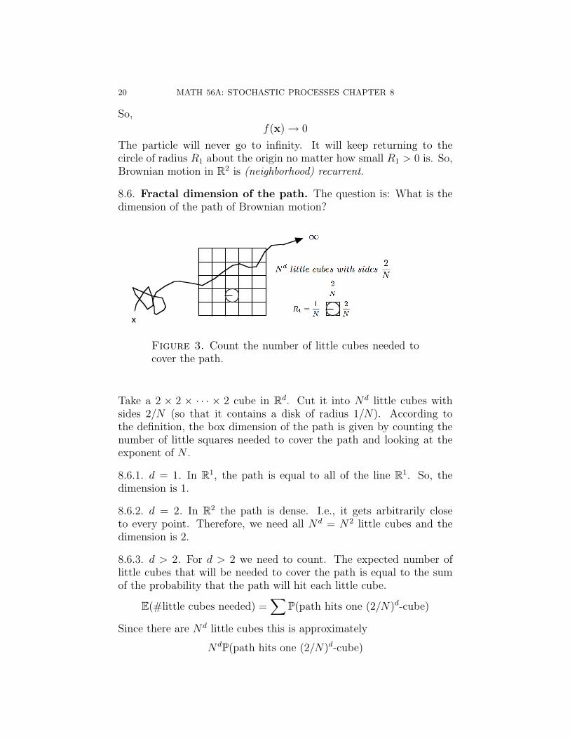
20 MATH 56A: STOCHASTIC PROCESSES CHAPTER 8
So,
f(x) → 0
The particle will never go to infinity. It will keep returning to thecircle of radius R1 about the origin no matter how small R1 > 0 is. So,Brownian motion in R2 is (neighborhood) recurrent.
8.6. Fractal dimension of the path. The question is: What is thedimension of the path of Brownian motion?
x
Figure 3. Count the number of little cubes needed tocover the path.
Take a 2 × 2 × · · · × 2 cube in Rd. Cut it into Nd little cubes withsides 2/N (so that it contains a disk of radius 1/N). According tothe definition, the box dimension of the path is given by counting thenumber of little squares needed to cover the path and looking at theexponent of N .
8.6.1. d = 1. In R1, the path is equal to all of the line R1. So, thedimension is 1.
8.6.2. d = 2. In R2 the path is dense. I.e., it gets arbitrarily closeto every point. Therefore, we need all Nd = N2 little cubes and thedimension is 2.
8.6.3. d > 2. For d > 2 we need to count. The expected number oflittle cubes that will be needed to cover the path is equal to the sumof the probability that the path will hit each little cube.
E(#little cubes needed) =∑
P(path hits one (2/N)d-cube)
Since there are Nd little cubes this is approximately
NdP(path hits one (2/N)d-cube)

MATH 56A: STOCHASTIC PROCESSES CHAPTER 8 21
But we have the formula for the probability that a point will hit asphere. So, I inserted the ratio between the volume of a cube and thevolume of a ball and I got:
Nd 2dΓ(
d+22
)πd/2
P(path hits ball of radius1
N)
We just calculated the probability of hitting the ball of radius R1 =1/N before going off to infinity. (This was when we took the limit asR2 →∞.) It was
P(hit ball of radius1
N) =
(R1
||x||
)d−2
=1
||x||d−2·N2−d
So the number of cubes needed is a constant times NdN2−d = N2. Sothe dimension of the path is 2.
8.7. Scaling and the Cauchy distribution. We skipped this be-cause we talked about scaling at the beginning of the chapter and Idon’t think we need to know the Cauchy distribution.
8.8. Drift. Brownian motion with (constant) drift in Rd is given by
Yt = Xt + µt
where µ ∈ Rd is a vector.Suppose we are given the information Ft up to time t. This is all
contained in the single vector Yt = x in the sense that
Ex(−) = E(− |Yt = x) = E(− |Ft)
ThenYt+δt = Xδt + µδt+ x
where Xδt is a recentered standard Brownian motion.Suppose that f(x) is the particle density at x at time t. (Density is
actually f(t,x) where the time t is just not written.)Here I converted to d = 1. Then
f(Yt+δt) = f(x)+f ′(x)(Xδt+µδt)+1
2f ′′(x)(Xδt+µδt)
2+o((Xδt+µδt)2)
I denoted the change in f by
δf = f(Yt+δt)− f(x)
So, the expected value of this is
Ex(δf) = f ′(x)Ex(Xδt + µδt) +1
2f ′′(x)Ex((Xδt + µδt)2) + o
The first expected value is
Ex(Xδt + µδt) = µδt

22 MATH 56A: STOCHASTIC PROCESSES CHAPTER 8
Next, I used the formula E(Z2) = E(Z)2 + V ar(Z) to get
Ex((Xδt + µδt)2) = Ex(Xδt + µδt)2 + V ar(Xδt + µδt)
= (µδt)2 + V ar(Xδt) + V ar(µδt)
= µ2δt2 + δt
and I pointed out that the term µ2δt2 is negligible since it is a o(δt).This also means that
o((Xδt + µδt)2) = o(µ2δt2 + δt) = o(δt)
and
Ex(δf(x)) = f ′(x)µδt+1
2f ′′(x)δt+ o(δt)
Dividing by δt and taking limit as δt→ 0 we get
f(x) = µf ′(x) +1
2f ′′(x)
where the dot is time derivative and the primes are space derivatives.This was for d = 1. In higher dimensions we get
∂f
∂t=
d∑i=1
µi∂f
∂xi
+1
2∆f

MATH 56A: STOCHASTIC PROCESSESCHAPTER 9
9. Stochastic integration
I will continue with the intuitive description of stochastic integralsthat I started last week.
9.0. the idea. I already talked about the probabilitistic and analyticapproach to Brownian motion. Stochastic integrals combine thesemethods. A key idea is Levy’s quadratic variation which is used inKunita and Watanabe’s [2] reformulation of stochastic integration.
9.0.1. quadratic variation. We want to define the stochastic integral
Zt =
∫ t
0
Ys dXs
where Xs is Brownian motion in R1. However, there is a big problembecause dXs has unbounded variation1. In other words,∫
|dXs| := limδt→0
∑|Xti+1
−Xti| = ∞.
Fortunately, we can still define the stochastic integral because the “qua-dratic variation” of Xt (denoted by 〈X〉t) is bounded:
Theorem 9.1 (Levy).
〈X〉t =
∫ t
0
(dXs)2 := lim
δt→0
∑(Xti+1
−Xti)2 = t
with probability one.
Proof. (p. 207) It is easy to see that the quadratic variation is approx-imately equal to t since the summands have expected value:
E((Xti+1−Xti)
2) = ti+1 − ti = δt
So the sum has expected value:
E(∑
(Xti+1−Xti)
2)
=∑
δt = t
Date: December 4, 2006.1The Riemann sum converges if and only the function has bounded variation.
1

2 MATH 56A: STOCHASTIC PROCESSES CHAPTER 9
The variance of each summand is2:
V ar((Xti+1−Xti)
2) = E((Xti+1−Xti)
4)− E((Xti+1−Xti)
2)2 = 2δt2
So, the sum have variance:
V ar(∑
(Xti+1−Xti)
2) =∑
2δt2 = 2tδt → 0
This means that, in the limit, the sum has zero variance and is thereforenot random. The value of this limit is almost sure equal to its expectedvalue which is t.
This theorem is usually written in the differential form
(9.1) (dXt)2 = dt
For arbitrary increments δt of t this is
(9.2) (δXt)2 := (Xt+δt −Xt)
2 = δt + oeff (δt)
where I labeled the error term as an effective little-oh. Usual: o(δt)/δt →0 as δt → 0. But effective little-oh means: If you take N ≈ 1/δt inde-pendent copies of oeff (δt) you get:
(9.3)∑
1/δt copies
oeff (δt) → 0 as δt → 0
These three equations (9.1), (9.2), (9.3) summarize the statementand proof of Levy’s theorem on quadratic variation of Brownian mo-tion.
9.0.2. Ito’s formula. Using quadratic variation we can “prove” Ito’sformula.
Suppose that we have a particle density function f(x) for x ∈ Rand Xt is Brownian motion. The probabilistic argument said that weshould look for the expected present value of f at the future position
2This is an easy calculation. The moment generating function for the standardnormal distribution is
E(eXt) =∫
ext−x2/2dx/√
2π = et2/2
∫e−(x−t)2/2dx/
√2π = et2/2
The coefficient of t2n in E(eXt) is E(X2n)/(2n)! and the coefficient of t2n in et2/2
is 1/n!2n. Therefore, for X ∼ N(0, 1),
E(X2n) =(2n)!n!2n
= (2n− 1)!! := 1 · 3 · 5 · 7 · · · (2n− 1)
You need to multiply by σ2n when X ∼ N(0, σ2).

MATH 56A: STOCHASTIC PROCESSES CHAPTER 9 3
Xt. So, we assume that f(x) is not time dependent. It only varies withposition x. Do you remember the following formula?
f(Xt+δt)− f(Xt) = f ′(Xt)(Xt+δt−Xt) +1
2f ′′(Xt)(Xt+δt−Xt)
2 + o(δt)
This can be abbreviated:
δf(Xt) = f ′(Xt)δXt +1
2f ′′(Xt)(δXt)
2 + o(δt)
Use quadratic variation: (δXt)2 = δt + oeff (δt). Then:
δf(Xt) = f ′(Xt)δXt +1
2f ′′(Xt)δt + oeff (δt)
Now take the sum from 0 to t. (We need to change t above to s so thats can be the variable going from 0 to t: 0 ≤ s ≤ t.)
f(Xt)− f(X0) =∑
f ′(Xs)δXs +∑ 1
2f ′′(Xs)δs +
∑oeff (δs)
Now, take the limit as δs → 0. Then the last term goes to zero by(9.3) and we get Ito’s formula:
(9.4) f(Xt)− f(X0) =
∫ t
0
f ′(Xs) dXs +
∫ t
0
1
2f ′′(Xs) ds
Here the stochastic integral is∫ t
0
f ′(Xs) dXs := limδs→0
∑f ′(Xs)δXs
9.0.3. discussion. Why is this not a proof of Ito’s formula? The mainthing is that we haven’t defined the stochastic integral:
Zt =
∫ t
0
Ys dXs
We only showed that the traditional “limit of Riemann sum” definitionmakes sense and gives something which satisfies Ito’s formula in thespecial case when Yt = f ′(Xt) is the derivative of a twice differentiablefunction of standard Brownian motion Xt. In general we need theintegral defined for predictable stochastic processes Ys. This means Ys
must be Fs-measurable and left continuous. Some people (e.g., ourbook) take Ys to be right continuous. However, following my “bible”[4], it makes more intuitive sense to have information (Xt and Ft) beright continuous and processes Yt based on this information should bepredictable.

4 MATH 56A: STOCHASTIC PROCESSES CHAPTER 9
9.1. discrete stochastic integrals. Stochastic integrals are constructedin three steps. First you have discrete time and finite state space (afinite Markov process). Then you have continuous time and finite statespace (a continuous Markov chain). Then you take a limit.
The important properties of the construction are visible at each step:
• The construction is linear.• The result is a martingale Zt.• Z2
t − 〈Z〉t is also a martingale where 〈Z〉t is the quadratic vari-ation of Zt.
Compare this with what you know about Brownian motion:
(1) Xt is a martingale.(2) X2
t − t is also a martingale.(3) 〈X〉t = t by Levy’s theorem which we just proved.
9.1.1. set up. Take simple random walk on Z. This gives a martingaleXn with X0 = 0 and increments Xn+1−Xn = ±1 with equal probability.Suppose that Yn is a predictable process, i.e., Yn is Fn−1-measurable.The discrete integral is
Zn :=n∑
i=1
Yi(Xi −Xi−1) =n∑
i=1
YiδXi
(This is supposed to resemble∫
Y dX.)The idea is that, at time n, you place a bet Yn+1 that Xn will increase.
The money that you win or lose at that step is
Yn+1(Xn+1 −Xn)
Since you cannot see the future, Yn+1 is only Fn-measurable.
9.1.2. linearity. This construction satisfies the following linearity con-dition: ∑
(aYi + bVi)δXi = a∑
YiδXi + b∑
ViδXi
In short, Zn is a linear function of Yi.
9.1.3. martingale.
Theorem 9.2. Zn is a martingale and Z0 = 0.
Proof. This is easy to verify:
E(Zn | Fn−1) = Zn−1 + E(Yn(Xn −Xn−1) | Fn−1)
Since Yn is Fn−1-meaaurable, the last term vanishes:
E(Yn(Xn −Xn−1) | Fn−1) = YnE(Xn −Xn−1 | Fn−1) = 0

MATH 56A: STOCHASTIC PROCESSES CHAPTER 9 5
So,E(Zn | Fn−1) = Zn−1
9.1.4. quadratic variation. The quadratic variation of Zn is just thesum of squares of differences:
〈Z〉n :=n∑
i=1
(Zi − Zi−1)2 =
∑Y 2
i
since these differences are
Zi − Zi−1 = Yi(Xi −Xi−1) = ±Yi
Theorem 9.3. Suppose that E(Y 2i ) < ∞ for each i. Then (Zn)2−〈Z〉n
is a martingale. In particular,
V ar(Zn) = E(Z2n) =
n∑i=1
E(Y 2i )
Proof. The difference between Z2n and the quadratic variation of Zn is
just the sum of the cross terms:
Z2n − 〈Z〉n = 2
∑1≤i<j≤n
YiYj(Xi −Xi−1)(Xj −Xj−1)
= Z2n−1 − 〈Z〉n−1 + 2
n−1∑i=1
YiYn(Xi −Xi−1)︸ ︷︷ ︸Fn−1-measurable
(Xn −Xn−1)︸ ︷︷ ︸E=0
So,E(Z2
n − 〈Z〉n | Fn−1) = Z2n−1 − 〈Z〉n−1

6 MATH 56A: STOCHASTIC PROCESSES CHAPTER 9
9.2. Integration wrt Brownian motion. We take Wt to be standardBrownian motion. This is also called the Wiener process, which mightexplain the use of the letter “W.” We want to define the integral
Zt =
∫ t
0
Ys dWs
where Ys is a predictable process (left continuous Ft-measurable) whichwe need to assume is square summable in the sense that
(9.5)
∫ t
0
E(Y 2s ) ds < ∞
for all t.
9.2.1. simple processes. The first step is to take a step function Yt.This is also called a simple predictable process. The book calls it a“simple strategy” to emphasize the assumption that Yt is given by aformula. “Simple” means that Yt takes only a finite number of values:0, Y0, Y1, · · · , Yn
Yt =
0 if t = 0
Y0 if 0 < t ≤ t1Y1 if t1 < t ≤ t2
· · ·Yn if tn < t
The stochastic integral is the function
(9.6) Zt =
∫ t
0
Ys dWs :=k∑
i=1
Yi−1(Wti −Wti−1) + Yk(Wt −Wtk)
if tk < t ≤ tk+1.
Remark 9.4. You can subdivide the intervals (ti−1, ti] and the integralZt remains the same. For example, if you insert t3/2 between t1 and t2and put Y3/2 = Y1 then
Y1(W2 −W1) = Y1(W3/2 −W1) + Y3/2(W2 −W3/2)
So the sum (9.6) remains the same after subdivision.
I want to go over the basic properties. Maybe I won’t prove them.
(1) Zt =∫ t
0Ys dWs is linear in Yt. I.e.,∫ t
0
(aXs + bYs) dWs = a
∫ t
0
Xs dWs + b
∫ t
0
Ys dWs
(2) Zt is a martingale which is square summable, i.e., E(Z2t ) < ∞.
(3) Z2t − 〈Z〉t is a martingale.

MATH 56A: STOCHASTIC PROCESSES CHAPTER 9 7
(4)
E(Z2t ) =
∫ t
0
E(Y 2s ) ds
(So, Zt is square summable if and only if Yt is square summable.)
Here the quadratic variation 〈Z〉t is given by
〈Z〉t =
∫ t
0
Y 2s ds
So, (3) ⇒ (4): If Z2t − 〈Z〉t is a martingale, then
E(Z2t − 〈Z〉t) = Z2
0 − 〈Z〉0 = 0
So,
E(Z2t ) = E(〈Z〉t) = E
(∫ t
0
Y 2s ds
)=
∫ t
0
E(Y 2s ) ds
Now, I am going to verify properties (2) and (3) (at least on paper).The key point is that all cross terms have expectation zero.
9.2.2. vanishing expectation of cross terms.
Theorem 9.5. Zt is a martingale for simple processes.
Proof. The definition of a martingale is that E(Zt | Fs) = Zs if s < t.By subdividing the interval, we can always assume that s is a jumptime (Remark 9.4). By induction it suffices to show this when s = tkis the last jump time before t. In other words, we have to show thatthe last term in Equation (9.6) has expectation 0:
E(Yk(Wt −Wtk) | Ftk) = YkE(Wt −Wtk | Ftk) = 0
The point is that this is a product where the first factor Yk is determinedwhen the second factor is still random with zero expectation.
And now, here is a wonderful theorem that will save us a lot of time:
Theorem 9.6 (Meyer). Suppose that Zt is a square summable martin-gale wrt Ft with Z0 = 0. Then Z2
t − 〈Z〉t is also a martingale.
In other words, (2) ⇒ (3)!
Proof. The idea is summarized in the following motto (from [1], 1.5.8).“When squaring sums of martingale increments and taking the expec-tation, one can neglect the cross-product terms.”
This theorem is supposed to proved property (3) in all cases simulta-neously. So, Zt could be anything. However, we can always subdivide

8 MATH 56A: STOCHASTIC PROCESSES CHAPTER 9
the interval [0, t] into parts of length δt and get Zt as a sum of incre-ments:
Zt = Zt − Z0 =∑
Zti − Zti−1=
∑δiZt
The increments δiZt = Zti − Zti−1have expectation zero since Zt is a
martingale. When you square Zt you get:
Z2t =
∑(δiZt)
2 + 2∑i<j
δiZtδjZt
The sum of squares converges to the quadratic variation by definition:
〈Z〉t := limδt→0
∑(δiZt)
2
and the cross terms δiZtδjZt have expectation zero because the firstterm is determined when the second term is random with expectationzero.
E(δiZtδjZt | Ftj−1) = δiZtE(δjZt | Fti) = 0
and by the rule of iterated expectation,
E(δiZtδjZt | Fs) = E(E(δiZtδjZt | Ftj−1) | Fs) = 0
for any s ≤ tj−1.
9.2.3. general stochastic integral (wrt Wt). Now suppose that Yt is any(square summable) predictable process. Then we convert to a simple
process by letting Y(n)s be the average value of Yt over the inverval
(k−1n
, kn] if s lies in the next interval ( k
n, k+1
n]. This is to insure that, at
time t = k/n when we choose Y(n)s , we only use information from the
past and not from the future, i.e., it is predictable.
Since Y(n)s is a simple predictable process, we can define
Z(n)t :=
∫ t
0
Y (n)s dWs
Without saying it, the book is using the following well-known theoremin real analysis applied to the measure space (Ω,Ft, P).
Theorem 9.7. The space of square summable real valued functions onany measure space is complete in the L2 metric.
The L2 metric is just
||Zt||2 := E(Z2t )
The martingales Z(n)t form a Cauchy sequence in the L2 norm. I.e.,
E((Z(n)t − Z
(m)t )2) = E(
⟨Z(n) − Z(m)
⟩t) =
∫ t
0
(Y (n)s − Y (m)
s )2 ds → 0
MATH 56A: STOCHASTIC PROCESSES CHAPTER 9 9
as n, m → ∞. The book then uses the theorem about completeness
of L2 to concluded that the martingales Z(n)t converge to some square
summable process Zt
Zt =
∫ t
0
Ys dWs := lim Z(n)t
Since the limit of martingales is a martingale, Zt is a martingale. ByTheorem 9.6 that is all we have to show (linearity being obvious).
9.3. Ito’s formula. I will repeat the formula and do the examples inthe book but I won’t go over the proof since we already did it.
Theorem 9.8 (Ito’s first formula). Suppose that Wt is standard Brown-ian motion and f(x) is C2, i.e., twice continuously differentiable. Then
f(Wt)− f(W0) =
∫ t
0
f ′(Ws) dWs +1
2
∫ t
0
f ′′(Ws) ds
I just want to point out that the naıve definition of the stochasticintegral that we used in the earlier proof of this formula is equivalentto the rigorous definition that I just explained because Yt = f ′(Wt) isa continuous function of t. Continuity implies that the average valueover an interval (used in the rigorous definition) converges to the actualvalue at one end (used in our naıve definition).
9.3.1. example 1. Let f(t) = t2. Then f ′(t) = 2t and f ′′(t) = 2. So,
f(Wt)− f(W0) = W 2t =
∫ t
0
2Ws dWs +1
2
∫ t
0
2 ds∫ t
0
Ws dWs =1
2W 2
t −1
2t
9.3.2. geometric Brownian motion. Take f(t) = et = f ′(t) = f ′′(t).Then Ito’s formula is:
eWt − 1 =
∫ t
0
eWs dWs +1
2
∫ t
0
eWs ds
If we write Xt := eWt this becomes:
Xt − 1 =
∫ t
0
Xs dWs +1
2
∫ t
0
Xs ds
or
dXt = Xt dWt +1
2Xt dt

10 MATH 56A: STOCHASTIC PROCESSES CHAPTER 9
9.4. Extensions of Ito’s formula. The key ideas are covariation andthe product rule.
9.4.1. covariation. This is also called the covariance process.
Definition 9.9. The covariation of At and Bt is defined to be
〈A, B〉t := limδt→0
∑δiA δiB
= limδt→0
∑(Ati − Ati−1
)(Bti −Bti−1)
Properties
〈A, A〉t = 〈A〉t (quadratic variation)
d 〈A, B〉t = dAtdBt (by definition)
〈A + B〉+ t = 〈A〉t + 〈B〉t + 2 〈A, B〉tQuick proof:∑
(δiA + δiB)2 =∑
(δiA)2 +∑
(δiB)2 + 2∑
δiAδiB
9.4.2. product rule. The following formula holds without error. (Seepicture.)
δAB = AδB + BδA + δAδB
Figure 1. The term δAδB becomes the covariation.
The infinitesmal version is
dAB = AdB + BdA + d 〈A, B〉t

MATH 56A: STOCHASTIC PROCESSES CHAPTER 9 11
Example 9.10. This is example 1 on p.209 which I also did at theend of the last section although I didn’t have time to do it in class. LetAt = Bt = Wt. Then
d 〈W, W 〉t = d 〈W 〉t = dt
So, the product rule gives:
dW 2t = 2Wt dWt + dt
9.4.3. quadratic variation of Zt. is equal to the quadratic variation ofthe stochastic part of Zt.
Lemma 9.11 (Lemma 1). If f is continuous with bounded variation(e.g. if f is differentiable) then
〈f〉t = 0
(The quadratic variation of f is zero.)
Proof.
〈f〉t = limδt → 0δf → 0
∑(δf)2 = lim
δf→0|δf |︸︷︷︸→ 0
∑|δf |︸ ︷︷ ︸
variation is bdd
= 0 · bdd = 0
Lemma 9.12 (Lemma 2). 〈f〉 = 0 ⇒ 〈f, X〉 = 0 ∀X.
Proof. If 〈f, X〉t > 0 then
〈X − af〉t = 〈X〉t − 2a 〈f, X〉t︸ ︷︷ ︸fixed >0
+ a2 〈f〉t︸ ︷︷ ︸0
If we make a really big then we can make 〈X − af〉t < 0. But this isimpossible because quadratic variations are sums of squares!
Here is the theorem we need:
Theorem 9.13. Suppose that
Zt =
∫ t
0
Xs ds +
∫ t
0
Ys dWs
where Xs integrable (i.e.,∫ t
0|Xs| ds < ∞). The second integral is the
“stochastic part” of Zt. Written infinitesmally:
dZt = Xt dt + Yt dWt
The theorem is:d 〈Z〉t = Y 2
t dt

12 MATH 56A: STOCHASTIC PROCESSES CHAPTER 9
Proof. Let f =∫ t
0Xs ds and g =
∫ t
0Ys dWs. Then Zt = f + g. So,
using the properties of covariation,
〈Z〉t = 〈f〉+ 〈g〉+ 2 〈f, g〉But, 〈f〉 = 0 by Lemma 1 (9.11) since f has bounded variation. And〈f, g〉 = 0 by Lemma 2 (9.12). So, 〈Z〉t = 〈g〉 and
d 〈Z〉t = (Yt dWt)2 = Y 2
t dt
9.4.4. Ito’s second formula. Suppose that f(x) is C2, i.e., twice con-tinuously differentiable. Then, the Taylor series of f gives is
(9.7) f(x + δx)− f(x) = f ′(x)δx +1
2f ′′(x)(δx)2 + o((δx)2)
Now, substitute x = Zt where Zt is as in the theorem above.
f(Zt+δt)− f(Zt) = f ′(Zt) δZt +1
2f ′′(Zt)(δZt)
2 + o
The infinitesmal version is:
df(Zt) = f ′(Zt) dZt +1
2f ′′(Zt) d 〈Z〉t
Substitute dZt = Xt dt + Yt dWt and d 〈Z〉t = Y 2t dt and we get:
Theorem 9.14 (Ito II).
df(Zt) = f ′(Zt)Xt dt + f ′(Zt)Yt dWt +1
2f ′′(Zt)Y
2t dt
9.4.5. Ito’s third formula. For this we need the vector version of theTaylor series (9.7) and we need to apply it to x = (t, Zt). Then f ′
becomes the gradient ∇f = (f1, f2) and
f ′(x) dx = (f1, f2)
(dtdZt
)= f(t, Zt) dt + f ′(t, Zt) (Xt dt + Yt dWt)
and f ′′ becomes the Hessian D2f =
(f11 f12
f21 f22
). So,
1
2f ′′(x)(dx)2 = (dt, dZt)
(f11 f12
f21 f22
) (dtdZt
)=
1
2f11 d 〈t〉︸︷︷︸
=0
+f12 d 〈t, Zt〉︸ ︷︷ ︸=0
+1
2f22d 〈Z〉t =
1
2f ′′(t, Zt)Y
2t dt
Putting these together we get:

MATH 56A: STOCHASTIC PROCESSES CHAPTER 9 13
Theorem 9.15 (Ito III).
df(t, Zt) = f(t, Zt) dt + f ′(t, Zt) (Xt dt + Yt dWt) +1
2f ′′(t, Zt)Y
2t dt
At this point we jumped ahead to the last section 9.8 on the Black-Scholes formula.
9.5. Continuous martingales. We skipped this section. But thislooks like a good place for me to put the proof of Levy’s theoremwhich implies that all continuous martingales are reparametrizationsof Brownian motion.
Theorem 9.16 (Levy). A continuous L2 martingale Mt starting at 0is standard Brownian motion if and only if M2
t − t is a martingale.
What follows is from Kunita and Watanabe [2] which is consideredto be the most elegant. I also included proofs of the necessary lemmas.
9.5.1. first step.
Lemma 9.17. Assuming the conditions of Theorem 9.16, 〈M〉t = t.
The proof of this lemma uses Meyer’s theorem proved in class that
Theorem 9.18 (Meyer). If Mt is a continuous L2 martingale then〈M〉t is the unique continuous increasing process starting at 0 so that
M2t − 〈M〉t
is a martingale.
Except that I didn’t prove the uniqueness and I didn’t define “in-creasing process.”
9.5.2. uniqueness of increasing process.
Definition 9.19. Xt is called an increasing process if
t > s ⇒ Xt ≥ Xs a.s.
(1) Clearly, Xt = t is a continuous increasing process.(2) 〈M〉t is an increasing process starting at 0 since
〈M〉t − 〈M〉s = limδt→0
∑(Mti −Mti−1
)2 ≥ 0
And 〈M〉t is continuous if Mt is continuous and square summa-ble (by definition of square summable).

14 MATH 56A: STOCHASTIC PROCESSES CHAPTER 9
Proof of uniqueness part of Meyer’s Theorem. Suppose that At, Bt arecontinuous increasing processes starting at 0 and
M2t − At, M2
t −Bt
are martingales. Then the difference
At −Bt
is also a continuous martingale starting at 0 with bounded variation(for t bounded). By the following lemma this implies that At = Bt. So,the continuous increasing process that we need to subtract from M2
t tomake it into a martingale is unique.
Lemma 9.20. Suppose Mt is a continuous martingale starting at 0and Mt has bounded variation for bounded t. Then Mt = 0 for all t.
Proof. By Lemma 1 (9.11), this implies that the quadratic variation ofMt is identically zero: 〈M〉t = 0. Therefore, M2
t is also a martingaleby the first part of Meyer’s theorem that we already proved in (9.6).But M2
t ≥ 0. So, E(Mt) = 0 only if Mt = 0 almost surely.
9.5.3. Kunita-Watanabe. One of the main results of [2] was to general-ize Ito’s formula to the case of L2 martingales. Or perhaps it would bemore fair to say that they formulated the theory of stochastic integralsin such a way that it easily extends to this case.
Theorem 9.21 (Kunita-Watanabe). If Mt is a continuous L2 martin-gale and f is C2 then
f(Mt)− f(M0) =
∫ t
0
f ′(Ms) dMs +1
2
∫ t
0
f ′′(Ms) d 〈M〉s
Now we can prove Levy’s theorem. Suppose that M2t − t is a mar-
tingale. We know that M2t − 〈M〉t is also a martingale. By Meyer’s
uniqueness theorem we can conclude that 〈M〉t = t.Now, let f(x) = eixz, f ′(x) = izeixz, f ′′(x) = −z2eixz where z is a
formal variable. Then f(Mt) = eiMtz and
E(eiMtz) = 1 + iE(Mt)z −1
2E(M2
t )z2 − i
3!E(M3
t )z3 +1
4!E(M4
t )z4 + · · ·
gives all of the moments of Mt. So, it suffices to show that thesemoments are what they should be if Mt were Brownian motion. I.e., itsuffices to show that
E(eiMtz) = e−tz2/2

MATH 56A: STOCHASTIC PROCESSES CHAPTER 9 15
But the Kunita-Watanabe variation of Ito’s formula gives:
E(f(Mt)− f(M0)) =1
2
∫ t
0
E(f ′′(Ms)) ds
since d 〈M〉s = ds and since anything predictable (like f(Ms)) timesdMs has expectation 0. Since f(M0) = e0 = 1 and f ′′(Ms) = −z2eiMtz
we have
E(eiMtz)− 1 =1
2
∫ t
0
−z2E(eiMsz) ds
Let h(t) = E(eiMtz). Then
h(t)− 1 =−z2
2
∫ t
0
h(s) ds
Differentiate both sides:
h′(t) =−z2
2h(t)
This is just exponential growth: h(t) = h(0)e−tz2/2. But h(0) = 1 sinceM0 = 0. So,
h(t) = E(eiMtz) = e−tz2/2
as claimed.
9.6. Girsanov transformation. We skipped this section.

16 MATH 56A: STOCHASTIC PROCESSES CHAPTER 9
9.7. Feynman-Kac. The formula of Feynman and Kac gives anotherway to solve the Black-Scholes equation. First we need to understandhow bonds grow if their rates are variable.
9.7.1. variable bond rate. Suppose the bond rate changes with time:r(t).Then the value of your bonds will grow by
(9.8) dYt = r(t)Yt dt
(9.9) Yt = Y0 exp
(∫ t
0
r(s) ds
)Why is (9.9) the solution of (9.8)?
Yt+dt = Y0 exp
(∫ t
0
r(s) ds +
∫ t+dt
t
r(s) ds
)= Yt exp(r(t)dt) = Yt(1 + r(t)dt + r(t)2dt2/2 + · · ·︸ ︷︷ ︸
=0
)
dYt = Ytr(t)dt
If we solve (9.9) for Y0 we get:
Y0 = Yt exp
(∫ t
0
−r(s) ds
)
9.7.2. the stochastic process. Now suppose we have a stochastic processZt satisfying the stochastic differential equation:
dZt = a(Zt)dt + b(Zt)dWt
Lemma 9.22. Zt is a martingale if and only if a(Zt) is identically zeroa.s.
Proof. Zt is a martingale iff E(dZt | Ft) = a(Zt)dt = 0
Let Jt be given by
Jt := exp
(∫ t
0
−r(s, Zs) ds
)This is how much one dollar at time t was worth at time 0 if the bondrate depends on time and on Zt.

MATH 56A: STOCHASTIC PROCESSES CHAPTER 9 17
9.7.3. the payoff. If the payoff function is f(ZT ) then the value at time0 of this payoff is
g(ZT )JT
How much of this value is determined by time t (0 ≤ t ≤ T )?
JT = exp
(∫ T
0
−r(s, Zs) ds
)
= exp
(∫ t
0
−r(s, Zs) ds +
∫ T
t
−r(s, Zs) ds
)= Jt exp
(∫ T
t
−r(s, Zs) ds
)9.7.4. the martingale.
Mt := E(g(ZT )JT | Ft)
= Jt E(g(ZT )exp
(∫ T
t
−r(s, Zs) ds
)| Ft)︸ ︷︷ ︸
V (t,Zt)
= JtV (t, Zt)
with MT = g(ZT ). This is a martingale by the law of iterated expec-tation:
E(Mt | Fs) = E(E(g(ZT )JT | Ft) | Fs) = E(g(ZT )JT | Fs) = Ms
Take the differential:
dMt = dJ V + J dV
= Jt(−r(t, Zt)V dt + Jt
(V dt + V ′ dZt +
1
2V ′′ d 〈M〉t
)= Jt(−r(t, Zt)V dt + Jt
(V dt + V ′a dt + V ′b dWt +
1
2V ′′b2 dt
)Since Mt is a martingale, the coefficient of dt must be zero (Lemma9.22) Therefore, if x = Ztthen
(9.10) −r(t, x)V (t, x) + V (t, x) + a(x)V ′(t, x) +b2(x)
2V ′′(t, x) = 0
(9.11) V (T, x) = g(x)

18 MATH 56A: STOCHASTIC PROCESSES CHAPTER 9
Theorem 9.23. The solution of the stochastic differential equation(9.10) with boundary condition (9.11) is given by
V (t, x) = Ex(g(ZT )exp
(∫ T
t
−r(s, Zs) ds
))
wheredZt = a(Zt) dt + b(Zt) dWt
9.7.5. application to Black-Scholes. If you apply this to the Black-Scholes equation (9.12) you get
r(t, x) = r
a(x) = rx
b(x) = σx
So,V (t, x) = Ex((ZT −K)+e−r(T−t))
dZt = rZt dt + σZt dWt
These equations say that the fair price of the option at time t is equalto the expected value of the option at time T adjusted for inflationassuming the stock has drift equal to the bond rate.

MATH 56A: STOCHASTIC PROCESSES CHAPTER 9 19
9.8. Black-Scholes.
9.8.1. the set-up.
St = value of one share of stock at time tdSt = µStdt + σSt dWt (= return)µ = drift (constant in this model)σ = volatility (also constant)Wt = standard Brownian motion
We are looking at a European call option. This is an option to buy oneshare of stock at price K at time T .
K = exercise price = strike priceT = expiry dateV (t, x) := fair price of the option at time t given that St = x
We want to calculate V (t, St). We know how much it will be worth atexpiry:
V (T, x) = (x−K)+ := max(x−K, 0)
But how much is the option worth today?
9.8.2. replicating portfolio. The theory is that there is a portfolio Ot
whose value at time T will be exactly (ST −K)+. Then the value of theoption should be the present value of the portfolio. Black and Scholesassumed that there are no arbitrage opportunities. This implies thatOt is unique. In [1] it says that there are always sure ways to losemoney. So, they don’t assume that the value of Ot is unique. Insteadit is proved that the fair price of the option is equal to the value of thecheapest replicating portfolio. Who is right is a matter of debate.
Fortunately, in this case, the replicating portfolio (also called a hedg-ing strategy) is unique.
Our portfolio is just a combination of stocks and bonds but we onlyhave one stock and one bond to choose from in this model. So,
Ot = XtSt + Yt
Xt = number of shares of stockYt = money in bondsr = bond rate (assumed constant)
The problem is to find Xt and Yt so that Ot = V (t, St) for all t ≤ T .Note: Ot needs to be self-financing. This means that we have to
continuously reinvest all profits. So, Ot grows in two steps:
(a) Stocks and bonds increase in value. (⇒ more $$)(b) You immediately reinvest the profit. (zero net gain in this step)

20 MATH 56A: STOCHASTIC PROCESSES CHAPTER 9
Step (a):
dOt = XtdSt + rYt dt
Step (b): Change Xt and Yt by dXt, dYt so that there is no net change
over what you got in step (a). Using the product rule this means:
dOt = XtdSt + rYt dt = SdXt + XtdSt + d 〈X, S〉t + dYt
We need to have V (t, St) = Ot. Using Ito’s third formula we get:
dV (t, St) = V (t, St) dt + V ′(t, St) dSt +1
2V ′′(t, St)σ
2S2t dt
= V (t, St) dt + V ′(t, St)µStdt + V ′(t, St)σStdWt︸ ︷︷ ︸stochastic part
+1
2V ′′(t, St)σ
2S2t dt
If this is equal to
dOt = XtdSt + rYt dt = XtµStdt + XtσStdWt︸ ︷︷ ︸stochastic part
+rYt dt
then the stochastic parts must be equal. So,
Xt = V ′(t, St)
Some people say it this way: If you are holding the option V (t, St) andyou sell off Xt = V ′(t, St) number of shares of stock then you havehedged away all of your risk (since the stochastic parts will cancel).Therefore, the financial instrument that you are holding: V (t, St)−XtSt
must be increasing in value at the bond rate which is exactly the case.Now go back to the equation dV (t, St) = dOt and cross out the terms
which are equal (XtdSt and V ′(t, St)dSt) and divide by dt. Then wehave:
rYt = V (t, St) +1
2V ′′(t, St)σ
2S2t
But we also know that
Yt = Ot −XtSt = V (t, St)− V ′(t, St)St
So,
V (t, St) +1
2V ′′(t, St)σ
2S2t − rV (t, St) + rV ′(t, St)St = 0
which we can rewrite as:
(9.12) V (t, x) +1
2σ2x2V ′′(t, x) + rxV ′(t, x)− rV (t, x) = 0
This is the Black-Scholes equation. This can be solved using Feynman-Kac. But it can also be solved directly using some tricks.
MATH 56A: STOCHASTIC PROCESSES CHAPTER 9 21
9.8.3. simplification of Black-Scholes equation. The first step is to no-tice that the drift µ does not matter. It is not part of Equation (9.12).Therefore, we may assume that µ = 0 and
(9.13) dSt = σSt dWt
The next step is: We may assume that r = 0. This is the same asmeasuring value in terms of value at time T adjusted for inflation.When r = 0 the equation becomes:
(9.14) V0(t, x) +1
2σ2x2V ′′
0 (t, x) = 0
When I say “we may assume r = 0” I mean that, if you can solve ther = 0 equation then you can also solve the original equation. Sup-pose V0(t, x) is the solution of this equation with boundary conditionV0(T, x) = (x−K)+. Then the solution of the original equation (9.12)is
(9.15) V (t, x) = e−r(T−t)V0(t, er(T−t)x)
The reason is that V0 is in terms of time T dollars and x dollars today(at time t) is worth er(T−t)x dollars at time T and the output V0 is interms of time T dollars. So, V0 of those dollars is worth e−r(T−t)V0 intoday’s dollars.
If you don’t believe it, you can just differentiate the expression in(9.15):
V = rV + e−r(T−t)V0 − rxV ′0
V = e−r(T−t)V0
V ′ = V ′0
V ′′ = er(T−t)V ′′0
Then
V +1
2σ2x2V ′′ + rxV ′ − rV
= (rV + e−r(T−t)V0 − rxV ′0) +
1
2σ2x2er(T−t)V ′′
0 + rxV ′ − rV
= e−r(T−t)V0 +1
2σ2x2er(T−t)V ′′
0 = 0

22 MATH 56A: STOCHASTIC PROCESSES CHAPTER 9
9.8.4. solution of Black-Scholes. Remember that µ = 0 = r. Thus
(9.16) dSt = σSt dWt
dV0(t, St) = dOt = XtdSt + rYt = XtσSt dWt
So, St, Ot, V0(t, St) are all martingales. Therefore,
V0(t, St) = E(V0(T, ST ) | Ft)
But T is the payoff date. So, we get
V0(T, x) = g(x) = (x−K)+ = max(x−K, 0)
where g(x) represents the payoff function. So, the value of the optionis just the expected payoff which will depend on the value of the stockat time T . So, we need to calculate ST .
Equation (9.16) can be solved for St as follows.
d ln St =dSt
St
+1
2
(−1
S2t
)σ2S2
t dt
= σ dWt −σ2
2dt
So,
ln St = σWt −σ2t
2+ C
Plugging in t = 0 gives C = ln S0. So,
St = S0exp
(σWt −
σ2t
2
)Now attach a little timer on the stock certificate and set that timer
to zero at time T − t. When the timer reaches t the expiry date hasarrived:
V0(T − t, x) = E(g(St) |S0 = x)
= E(g(x eσWt−σ2t/2)
)Letting y = x e−σ2t/2 we get:
V0(T − t, y eσ2t/2) = E((y eσWt −K)+
)But σWt ∼ N(0, σ2t). So we can use the following lemma with b =
σ√
t, a = y = x e−σ2t/2 = xe−b2/2.
Lemma 9.24. Suppose that X = aebZ where Z ∼ N(0, 1). Then theexpected value of g(X) = (X −K)+ is
E((X −K)+) = aeb2/2Φ
(ln(a/K) + b2
b
)−KΦ
(ln(a/K)
b
)where Φ is the distribution function for N(0, 1).

MATH 56A: STOCHASTIC PROCESSES CHAPTER 9 23
Theorem 9.25. The value of the European call option at time T − tis
V0(T − t, x) = xΦ
(ln(x/K) + σ2t/2
σ√
t
)−KΦ
(ln(x/K)− σ2t/2
σ√
t
)if St = x assuming the bond rate is zero and
V (T − t, x) = e−rtV0(t, ertx)
= xΦ
(ln(x/K) + rt + σ2t/2
σ√
t
)− e−rtKΦ
(ln(x/K) + rt− σ2t/2
σ√
t
)if the bond rate is a constant r.
Proof of Lemma 9.24. The expected value is given by an integral whichis easy to compute:
E((aebZ −K)+) =
∫ ∞
−∞(aebz −K)+φ(z) dz
Since aebz = K when z = 1bln(K/a) we can write this as:∫ ∞
1b
ln(K/a)
aebz−z2/2 −Ke−z2/2 dz√2π
For the first part you can change variables by z = y + b, dz = dy to get∫ ∞
1b
ln(K/a)
aebz−z2/2 dz√2π
=
∫ ∞
1b
ln(K/a)−b
aeb2/2−y2/2 dy√2π
Changing y to −y this gives
aeb2/2
∫ 1b
ln(a/K)+b
−∞e−y2/2 dy√
2π= aeb2/2Φ
(1
bln(a/K) + b
)The second term is easy:∫ ∞
1b
ln(K/a)
−Ke−z2/2 dz√2π
= −K
(1− Φ
(1
bln(K/a)
))
= −KΦ
(1
bln(a/K)
)
I’ll stop here. (But in the lecture I have to go back to section 9.7 onthe Feynman-Kac formula.)
“The one thing probabilists can do which analysts can’t is stop...”-Sid Port, analyst [3]

24 MATH 56A: STOCHASTIC PROCESSES CHAPTER 9
References
1. Ioannis Karatzas and Steven E. Shreve, Brownian motion and stochastic calculus,second ed., Graduate Texts in Mathematics, vol. 113, Springer-Verlag, New York,1991.
2. H. Kunita and S. Watanabe, On square integrable martingales, Nagoya Math. J.30 (1967), 209–245.
3. L. C. G. Rogers and D. Williams, Diffusions, Markov processes, and martingales.Vol. 1, second ed., Wiley Series in Probability and Mathematical Statistics:Probability and Mathematical Statistics, John Wiley & Sons Ltd., Chichester,1994, Foundations.
4. L. C. G. Rogers and David Williams, Diffusions, Markov processes, and mar-tingales. Vol. 2, Cambridge Mathematical Library, Cambridge University Press,Cambridge, 2000, Ito calculus, Reprint of the second (1994) edition.


![· 216 KIYOSHI IGUSA Proof. It su ces to take n=0sinceZ[0] maps to Z[n] for all n. If P is empty or contains only one element then there is a unique morphism P ! Z[0] so suppose](https://static.documents.pub/doc/80x56/6015683085fbeb6c746f0c93/216-kiyoshi-igusa-proof-it-su-ces-to-take-n0sincez0-maps-to-zn-for-all-n.jpg)
