Page 1
Faculty of Engineering
Department of Mechanical Engineering
KMEM4214 APPLIED VIBRATION
Session 2013/2014
Semester I
COOPERATIVE LEARNING (CL) ASSIGNMENT 3
Group 3
NAME: MATRIC NUMBER:
KOAY KAH LOON KEM100016
DZULBADLY BIN ABD MANAP KEM100011
FARAHTUL AIN BINTI MUSA KEM100014
LEE CHIA CHUN
LEE HANJUNE
KEM100017
KEM100018
Name of Lecturer : DR. ONG ZHI CHAO
Page 2
i
ABSTRACT
In this assignment, two different experimental techniques are used to analyze the vibration on
mobile simulation rig, in single Z-direction only. In modal analysis experiment, the FRF
(Frequency Response Function) of system is determined while the Operational Deflection
Shape (ODS) analyzes the dynamic characteristics of a structure under actual operating
conditions. The experiment was then carried out after the expected result is determined from
ODS. MDTQ2 Data Acquisition System and ME’scope were used for both experiments. The
impact frequency of the shaker was set to 20.25 Hz in ODS. For modal analysis experiment,
the accelerometer was set at fixed point of the rig after the apparatus has been set up in order
to measure the dynamic characteristics of the simulation rig. Impact hammer was used to knock
at each point of the rig, a total of 15 points were knocked throughout the experiment. While
knocking at each of the point, we actually applying force as our input and the dynamic response
were read through DASYLab software, which is our output. FRF (Frequency Response
Function) can be calculated since we have input (force) and output (displacement). Then, in
Modal Analysis, the damped frequency, damping ratio percentage and decay rate were obtained
through curve fitting on ME’scope software. Unlike Modal Analysis experiment, the force
acting on the rig or input are not measured in operational deflection shape (ODS) analysis
experiment; thus unknown. However, we use a shaker to apply periodic excitation as our input.
We can consider it is as damped response to periodic excitation. We use two accelerometer in
this experiment. One of accelerometer was set at fix point on rig while the other was roved at
each point on the rig. The task was to measure the mode on point 3 of the rig. ME’scope
software was used to animate the shape after the data have been obtained through DASYLab.
Since the response can be consider as damped response to periodic excitation, we use the
formula to calculate the response. Matrix calculation and animation of the mode shape were
done by using MatLab. The results were compared between ODS and Modal Analysis, and
were subsequently discussed.
Page 3
ii
Table of Contents
ABSTRACT ................................................................................................................................ i
1.0 INTRODUCTION .......................................................................................................... 1
1.1 Operational Deflection Shape (ODS) .......................................................................... 1
1.2 Experimental Modal Analysis (EMA) ........................................................................ 3
2.0 THEORETICAL BACKGROUND ................................................................................ 4
3.0 METHODOLOGY ......................................................................................................... 6
3.1 Experimental Procedure .............................................................................................. 6
3.2 Experimental Set-Up ................................................................................................... 7
3.3 Procedures of Post-Processing Using ME’Scope........................................................ 9
3.3.1 Modal Analysis .................................................................................................... 9
3.3.2 Operational Deflection Shape (ODS) ................................................................ 23
3.4 Methodology ............................................................................................................. 24
4.0 RESULTS AND DISCUSSIONS ................................................................................. 25
4.1 Calculation ................................................................................................................ 25
4.2 Discussion ................................................................................................................. 38
4.3 Possible Sources of Errors and Precautions .............................................................. 42
5.0 Conclusion .................................................................................................................... 43
Page 4
1
1.0 INTRODUCTION
Vibration is the result of energy being transferred back and forth between kinetic and potential
energies. There are different experimental techniques that can be used to analyse vibrations.
The most common techniques are experimental modal analysis and operational deflection
shape analysis. In experimental modal analysis, the exaction of dynamic behaviour of a
structure can be determined. In operational deflection shape analysis the vibration shapes under
real operating conditions can be determined.
1.1 Operational Deflection Shape (ODS)
Operational Deflection Shape (ODS) analysis is a measurement process of determining the
motion of a structure while it is in operation. ODS analysis is the linear combination of the
mode shape at a specific frequency. The contribution of the modes depends on the frequency
and location of the excitation forces.
In this experiment for our group (Group 3), the excitation location will be on the point
3 with the excitation frequency of 20.25 Hz. It is different from mode shapes, in the sense that
operating deflection shapes can be scaled to absolute engineering units such as inches while
mode shapes are scaled in relative units. The actual motion is too fast and the amplitude is too
small to be visualized by our naked eyes. ODS with help of ME’Scope (a post-processing
vibration software) analysis provides a picture of how a machine or structure moves in actual
operation at specific frequencies of interest and helps the user to determine the cause of the
motion using some digital signal processing technique. Typically, these frequencies will be
running speeds, harmonics, gear mesh frequencies, etc. or a unique frequency that exhibits an
objectionable response. The ODS extraction can be performed using both frequency domain
and time domain.
In ODS analysis the vibration shapes of a structure, under operating conditions, are
determined. The output of the system can be any number of things such as displacement,
accelerations and others. In contrary to modal analysis, the forces acting on the system or inputs
are not measured and, thus unknown.
ODS analysis in frequency domain can be obtained in the similar way as in
Experimental Modal Analysis (EMA) but by using displacements at both input and output. It
is performed while the machine is operating. ODS analysis utilizes the Frequency Response
Function (FRF) measurements to determine the actual deflection of a structure or a system
Page 5
2
under steady state operating condition. It is a measurement technique that is very similar to
EMA but both channels are attached with accelerometer. Instead of using an excitation force,
response at one location is used as a reference. So, a minimum of two accelerometers are
required to measure vibration signal over a selected frequency range; one of the accelerometers
remains fixed while the other unit is moved throughout the selected points on the structure.
Roving tri-axial accelerometers are used to collect the dynamic response with respect to the
reference location. The roving accelerometer will be attached by using magnet and a square
block to enable it to make measurement in three axes. The relative amplitude and phase is
calculated for each of the roving response accelerometer locations with respect to the reference
accelerometer.
ODS analysis using time waveform requires “n” sets of accelerometers and a minimum
n-channel data acquisition system, where n equals to the number of required degree of freedom
for the structure to be analysed. The time waveform of all signals is synchronously recorded.
Assigning each waveform to a particular freedom node in a structure and scanning through all
the time trace synchronously will generate the operating deflection shape of the structure. This
is ideal for analyzing signals that are not in steady-state, such as the transient response.
In ODS analysis the vibration shapes of a structure, under operating conditions, are
determined. The output of the system can be any number of things such as displacement,
accelerations and others. On contrary to modal analysis, the forces acting on the system or
inputs are not measured and, thus unknown.
The advantages of ODS with respect to modal analysis are:
there is no assumption of a linear model
the structure experiences actual operating forces
true boundary conditions apply
The disadvantages with respect to modal analysis are:
no complete dynamic model is obtained, so no natural frequencies, mode shapes and
damping properties can be determined
operational deflection shapes only reflect the cyclic motion at a specific frequency, but
no conclusions can be drawn for the behaviour at different frequencies
Page 6
3
1.2 Experimental Modal Analysis (EMA)
The dynamic properties of a structure can be determined by FEM modal-simulations (Finite
Element Method), or by experimental modal analysis. As the machine already has been built,
an experimental approach is chosen. In experimental modal analysis, the FRF (Frequency
Response Function) of a system is determined. The FRF is a model of a linear system. It is the
relationship between the measured output (e.g. displacement) and input (e.g. force), as a
function of frequency. When both the applied force and the response to it are measured
simultaneously, the FRF can be calculated. From this FRF, the natural frequencies, mode
shapes and modal damping can be obtained.
In modal analysis an important assumption is that the measured structure is isolated from
its surroundings, so that no external forces are acting on the system. Considering the size of the
one-man ride machine, it is very difficult to isolate it from its environment. Moreover, there is
no equipment available to simultaneously apply and measure input forces of this (high) level.
Therefore, it is chosen to determine the vibration shapes under operating conditions, using
operational deflection shape analysis.
Page 7
4
2.0 THEORETICAL BACKGROUND
If a lightly damped system is subjected to a set of actions that all proportional to the simple
harmonic function cos𝜔𝑡 , the action vector Q may be written as:
Q = P cos𝜔𝑡 (1)
Where,
(2)
Transformation of the action equations of motion to normal coordinates produces the typical
modal equation
(3)
where r = 1, 2, 3…….n
The damped steady-state response of the rth mode is
(4)
with Equation (4) can be expressed in terms of magnitude and phase as
(5)
in which the magnification factor 𝛽r is
(6)
Page 8
5
and the phase angle, 𝜃r is
(7)
To determine the response of each mode using the respective modal column from Equation 8
(8)
Back transformation to obtain the contribution of the considered mode
(9)
All the values for the natural frequency (ωₒ), damped frequency (ωd), decay rate (σ), are
determined from the formulas as follows:
: Decay rate (10)
: Damped natural frequency (11)
Page 9
6
3.0 METHODOLOGY
3.1 Experimental Procedure
The automobile simulation rig was used to study its dynamic characteristics under two
conditions, namely non-operating and operating conditions. Modal analysis, to be precise is
Experimental Modal Analysis (EMA) was used to investigate the modal parameters, namely
natural frequencies, damping and mode shapes while the rig was subject to non-rotating
condition whereas Operational Deflection Shape (ODS) was adopted for the rig under rotating
condition, so as to obtain a reference set of modal parameters for the modal analysis. The modal
parameters obtained from ODS were made as benchmark set and the modal parameters
obtained from EMA were compared to that of ODS.
The automobile simulation rig has a total of 15 points marked on its surface. Vibrations
were artificially introduced by impact hammer in EMA whereas a shaker was used in ODS to
generate a continuous wave of vibration at a specified impact frequency. The vibration speed
of a shaker was regulated by a controller that has a adjust knob to set the impact frequency. A
National Instrument (NI) dynamic analyser was used to receive the analogue signals resulted
from the vibration, and converted the analogue signals into digital signal. The signals were
stored, monitored and controlled by DasyLab, which is processing software. Various
operations were performed such as averaging, filtering, windowing function and Fast Fourier
Transform in the time domain of the signal.
Vibration was imparted at each point marked on the surface of the simulation rig. In
EMA, 5 averages of impact were taken on each point using impact hammer whereas in ODS,
a total of 10 averages were taken for ODS while shaker was in operation.
After that, the results obtained from both EMA and ODS were saved in ASCII format.
ME’Scope post-processing software performed curve-fitting for EMA. After assigning
sufficient points to describe the structure vibrational responses, ME’Scope would animate the
mode shapes of the structure.
Page 10
7
3.2 Experimental Set-Up
Table 0.1: List of Instruments
Instruments Descriptions
Automobile Simulation Rig Used as test rig to perform EMA & ODS
Shaker On when performing ODS to create ambient excitation
PCB Impact Hammer
(Model 086C03)
Sensitivity: 2.16 mv/N
Tip type: medium tip with vinyl cover
Hammer mass: 0.16 kg
Frequency range: 8kHz
Amplitude range: ±2200 N peak
IMI Tri-axial
Accelerometer
(Model 604B31)
To measure the response acceleration at a fixed point and
direction
Sensitivity: 100 mv/g
Frequency range: 0.5 – 5000 Hz
Amplitude range: ±50 g peak
NI USB Dynamic Signal
Acquisition Module,
(Model NI-USB 9234)
Number of channels: 4
ACD resolution: 24 bits
Minimum data rate: 1650 samples/sec
Maximum data rate: 51200 samples/sec
DASYLab v10.0 Sampling rate: 2048 samples/sec
Block size: 4096
EMA:
Channel 1: Impact Hammer (EMA)
Channel 2: Accelerometer (Z-axis) [Green]
ODS:
Channel 1: Sensor (at a fixed point)
Channel 2: Sensor (roving from point 1 to 15)
Channel 4: Force sensor connected to the shaker
Application of exponential window in time response, at a
decay rate of 3. Adjustment was made in Pre-Setting
mode before switching into Modal Main.
Page 11
8
Table 3.1 (cont’d): List of Instruments
ME’Scope v4.0 To process collected data from NI-
DASYLab
To define the structural geometry for modal
analysis
To determine the natural frequencies,
damping and animated mode shapes. Curve-
fitting process was done only on the FRF of
EMA, no curve fitting was done on the FRF
of ODS.
Figure 3.0: User interface of ME’Scope
Page 12
9
3.3 Procedures of Post-Processing Using ME’Scope
This section explains the step-by-step procedures on using ME’Scope to determine the dynamic
characteristics of the test subject, namely natural frequencies, damping and mode shapes. The
data obtained from Modal Analysis and Operational Deflection Shape (ODS) will be processed
separately by using ME’Scope. The difference in terms of procedures lies on the curve-fitting
function, data obtained from ODS do not require to perform curve-fitting whereas data obtained
from Modal Analysis will be performed with curve-fitting. Both outcomes will give an
animation of how the structure vibrates, as well as obtaining the dynamic characteristics.
3.3.1 Modal Analysis
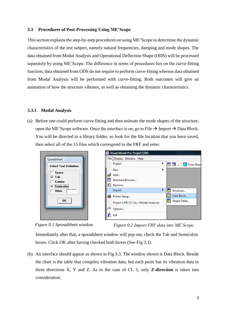
(a) Before one could perform curve-fitting and then animate the mode shapes of the structure,
open the ME’Scope software. Once the interface is on, go to File Import Data Block.
You will be directed to a library folder, so look for the file location that you have saved,
then select all of the 15 files which correspond to the FRF and enter.
Immediately after that, a spreadsheet window will pop out, check the Tab and Semicolon
boxes. Click OK after having checked both boxes (See Fig 3.1).
(b) An interface should appear as shown in Fig 3.3. The window shown is Data Block. Beside
the chart is the table that compiles vibration data, but each point has its vibration data in
three directions X, Y and Z. As in the case of CL 3, only Z-direction is taken into
consideration.
Figure 0.2 Import FRF data into ME’Scope Figure 0.1 Spreadsheet window
Page 13
10
Figure 0.3 Interface
Figure 0.4 Data block window. Each point has vibration data for X, Y & Z directions.
In order to only focus on vibration data correspond to Z-direction, go to Edit Select
Traces By, as shown in Fig. 3.5. A “Select Traces” window will pop-up window, choose
“Direction”, then select “Z”. Hit the “Select” button” and Close the pop-up window. After
having done this step, the vibration data at the points (15 points in total) correspond to Z-
direction will be highlighted in green, as shown Fig. 3.6.
Page 14
11
Figure 0.5 Select vibration data of each point correspond to Z-direction only
Figure 0.6 Select Traces pop-up window. Choose “Direction” and then select “Z”.
Copy the highlighted points into a new data block window by going to Edit Copy
Traces. A new data block window will open. The previous data block window can be deleted.
See Figure 3.7.
Page 15
12
Figure 0.7 After copying traces, two data block windows will appear. Delete the previous
data block window, and consider the new window that consists of vibration points of interest
(c) The new data block window consists of all 15 points of interest in Z-direction. Next, double
click at magnitude (vertical axis label), a “Vertical Axis” window would pop up, under the
Linear/Log pane, select “Linear”, as shown in Fig. 3.8. Then, double click at Hz
(horizontal axis label), a “Horizontal Axis” window would pop up, as shown in Fig. 3.9.
Under the “Display Limits” panel, set 0 and 100 as Starting Value and Ending Value
respectively.
Figure 0.8 Vertical Axis window pops up. Pick “Linear” under Linear/Log pane.
Page 16
13
Figure 0.9 Horizontal Axis window pops up. Starts 0 as Starting Value and 100 Ending Value
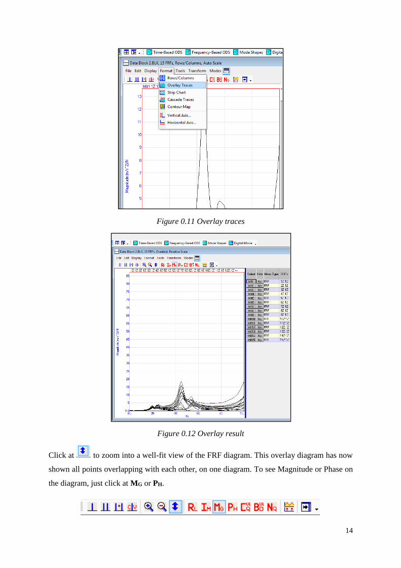
(d) After changing the settings at both vertical and horizontal axis, the FRF diagram should
look roughly like that as shown in Fig. 3.10. Note that the diagram is now showing only
vibration data of only ONE of the points. To overlay all of the curves together, go to
Format Overlay Traces as shown in Fig. 3.11. Consequently, the curves will be overlaid
as shown in Fig. 3.12.
Figure 0.10
Page 17
14
Figure 0.11 Overlay traces
Figure 0.12 Overlay result
Click at to zoom into a well-fit view of the FRF diagram. This overlay diagram has now
shown all points overlapping with each other, on one diagram. To see Magnitude or Phase on
the diagram, just click at MG or PH.
Page 18
15
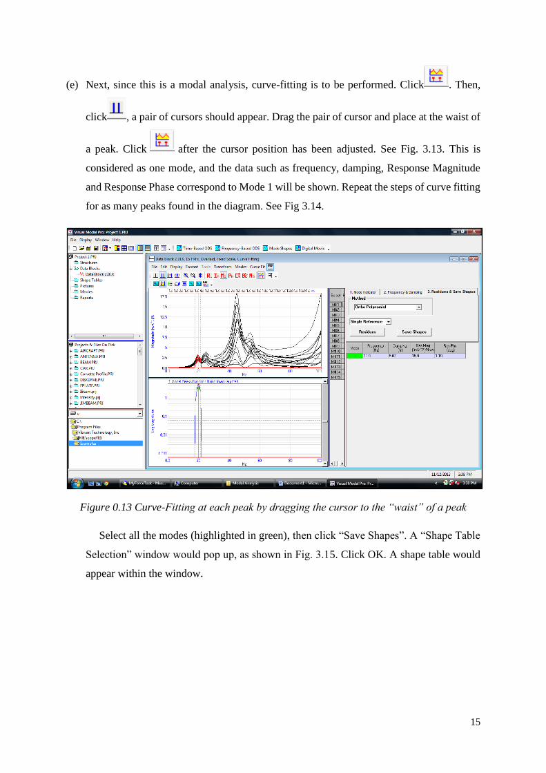
(e) Next, since this is a modal analysis, curve-fitting is to be performed. Click . Then,
click , a pair of cursors should appear. Drag the pair of cursor and place at the waist of
a peak. Click after the cursor position has been adjusted. See Fig. 3.13. This is
considered as one mode, and the data such as frequency, damping, Response Magnitude
and Response Phase correspond to Mode 1 will be shown. Repeat the steps of curve fitting
for as many peaks found in the diagram. See Fig 3.14.
Figure 0.13 Curve-Fitting at each peak by dragging the cursor to the “waist” of a peak
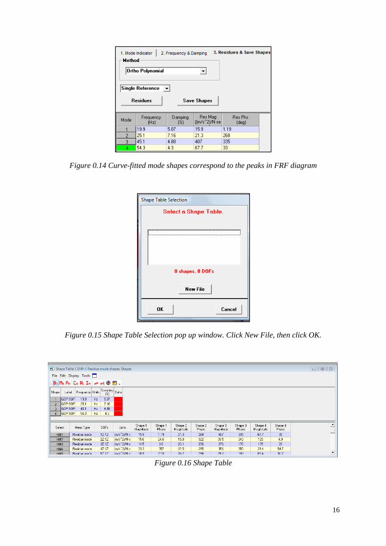
Select all the modes (highlighted in green), then click “Save Shapes”. A “Shape Table
Selection” window would pop up, as shown in Fig. 3.15. Click OK. A shape table would
appear within the window.
Page 19
16
Figure 0.14 Curve-fitted mode shapes correspond to the peaks in FRF diagram
Figure 0.15 Shape Table Selection pop up window. Click New File, then click OK.
Figure 0.16 Shape Table
Page 20
17
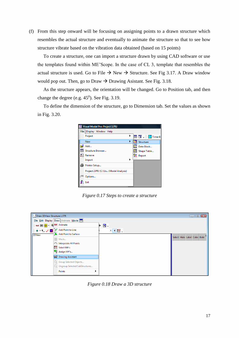
(f) From this step onward will be focusing on assigning points to a drawn structure which
resembles the actual structure and eventually to animate the structure so that to see how
structure vibrate based on the vibration data obtained (based on 15 points)
To create a structure, one can import a structure drawn by using CAD software or use
the templates found within ME’Scope. In the case of CL 3, template that resembles the
actual structure is used. Go to File New Structure. See Fig 3.17. A Draw window
would pop out. Then, go to Draw Drawing Asistant. See Fig. 3.18.
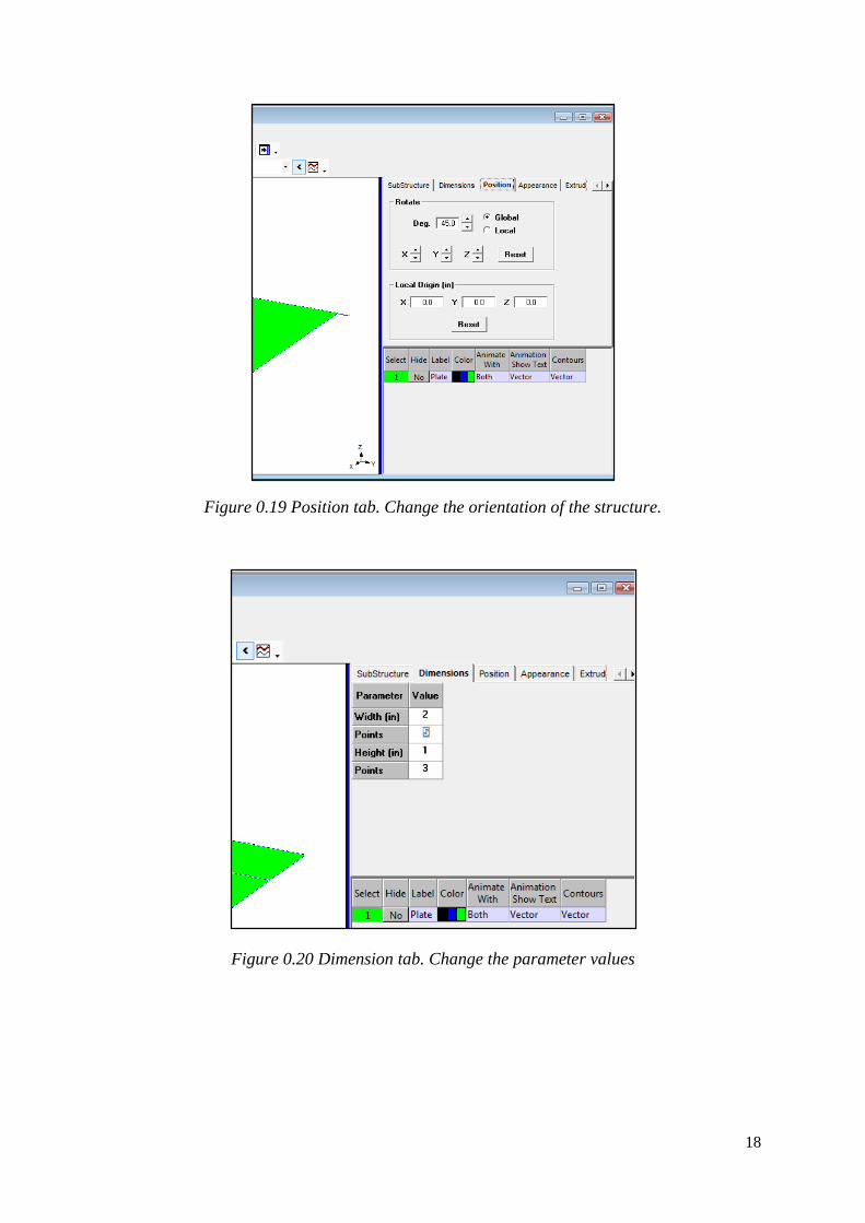
As the structure appears, the orientation will be changed. Go to Position tab, and then
change the degree (e.g. 450). See Fig. 3.19.
To define the dimension of the structure, go to Dimension tab. Set the values as shown
in Fig. 3.20.
Figure 0.17 Steps to create a structure
Figure 0.18 Draw a 3D structure
Page 21
18
Figure 0.19 Position tab. Change the orientation of the structure.
Figure 0.20 Dimension tab. Change the parameter values
Page 22
19
Next, is to assign points on the simulated structure. Go to Draw Assign MPs, as
shown in Fig. 3.21. A “Animation Source” window would pop out, as shown in Fig. 3.22.
Select the Data Block file that contains all of the vibration data.
Figure 0.21
Figure 0.22
Page 23
20
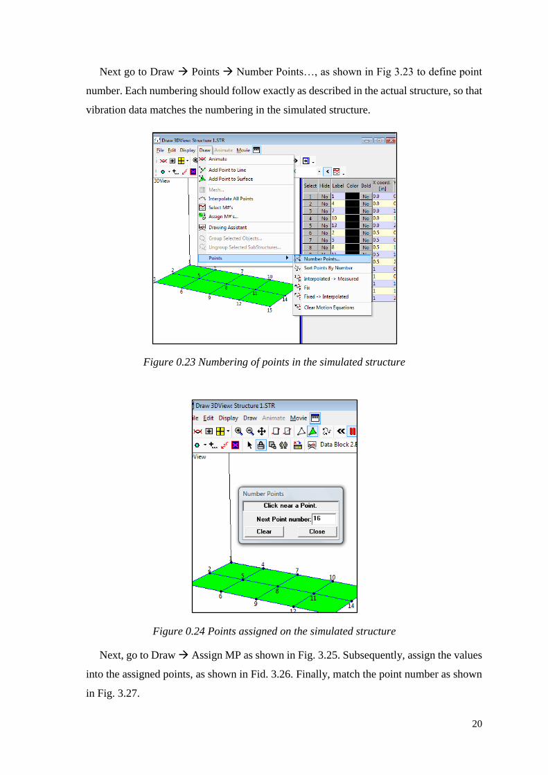
Next go to Draw Points Number Points…, as shown in Fig 3.23 to define point
number. Each numbering should follow exactly as described in the actual structure, so that
vibration data matches the numbering in the simulated structure.
Figure 0.23 Numbering of points in the simulated structure
Figure 0.24 Points assigned on the simulated structure
Next, go to Draw Assign MP as shown in Fig. 3.25. Subsequently, assign the values
into the assigned points, as shown in Fid. 3.26. Finally, match the point number as shown
in Fig. 3.27.
Page 24
21
Figure 0.25
Figure 0.26 Assign values in Data Block to the Assigned Points
Figure 0.27 Match the point number to the vibration data obtained
Page 25
22
Figure 0.28 Overview after finished assigning points.
(g) To animate the structure, click found in the panel. The structure has now been
animated. The mode shapes can be visually shown. See Fig. 3.29. If the frequency is
changed by means of dragging the cursor in the FRF diagram, the structure would vibrate
differenty.
(h) Save the animation in video format. Go to Movie Saved as video (Quod view
preferrable)
Figure 0.29 Animated (Quod View) window
Page 26
23
3.3.2 Operational Deflection Shape (ODS)
(a) ODS vibration data spectrum is rather simpler to be analysed and animated, as its data does
not require curve-fitting. Follows the step from (a) to (d) in section 3.3.1 Modal Analysis.
(b) To animate the structure, follows steps from (f) to (g) in section 3.3.1 Modal Analysis.
(c) Save the animation in video format.
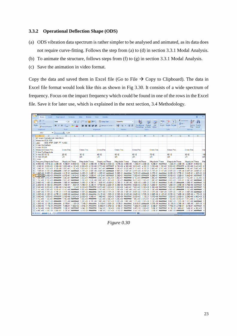
Copy the data and saved them in Excel file (Go to File Copy to Clipboard). The data in
Excel file format would look like this as shown in Fig 3.30. It consists of a wide spectrum of
frequency. Focus on the impact frequency which could be found in one of the rows in the Excel
file. Save it for later use, which is explained in the next section, 3.4 Methodology.
Figure 0.30
Page 27
24
3.4 Methodology
Previous sections concerns about the experimental procedures to obtain and analyse the data.
This section explains how the data and analysis are being used to explain the nature.
Firstly, obtains the damping ratio, ϛ and decay rate, σ needs to be calculated the natural
frequency using the relation σ = ϛ𝝎𝒏 and 𝝎𝒅 = 𝝎𝒏√𝟏 − 𝜻𝟐, where 𝜔𝑛 is natural frequency
and 𝜔𝑑 is damped natural frequency. With the known input force, Q, which is 0.17N and the
calculation using analytical method used in Modal Analysis, the response can be obtained.
Secondly, sum up all values of the magnitude and phase (together with its sign)
throughout the 15 points (from 1z to 15Z) respectively, which correspond to the impact
frequency, in the case, is 20.25 Hz.
The highlighted row in Fig. 3.31 shows the experimental impact frequency (20.25 Hz)
and the corresponding damping and mode shapes.
Figure 0.31
Finally, these values from both Modal Analysis and Operational Deflection Shape
(ODS) are to be compared.
Page 28
25
4.0 RESULTS AND DISCUSSIONS
4.1 Calculation
The eigenvector (φ), damping ratio (Ϛ) in percentage and the damped frequency (ωd) in Hz
obtained from the data of the modal analysis as well as the excitation force (Q) and excitation
frequency (ω) obtained from ODS are as follows:
Table 4.1: Results obtained from Modal Analysis
Frequency, ωd (Hz) Damping (%) Damping ratio, Ϛ Excitation frequency, ω
20 5.26 0.0526 20.25 Hz
127.235 rad/s 25.1 7.16 0.0716
45.1 4.94 0.0494
54.3 4.36 0.0436
Eigenvector, φ = 0.362 0.367 1.22 -0.491 Q = 0
0.343 0.272 0.0702 -0.789 0
0.337 0.449 -0.827 -1.05 0.17
0.554 0.559 1.08 -0.247 0
0.452 0.63 -0.086 -0.521 0
0.464 0.692 -1.03 -0.906 0
0.721 1.14 0.978 0.331 0
0.666 0.99 -0.146 -0.136 0
0.65 1.02 -1.37 -0.56 0
0.685 0.928 0.803 0.866 0
0.524 0.733 -0.301 0.369 0
0.644 0.82 -1.62 -0.225 0
0.575 0.381 0.589 1.23 0
0.512 0.361 -0.414 0.854 0
0.478 0.331 -1.45 0.478 0
By using Microsoft Excel, the values for the natural frequency (ωₒ), modal decay rate (σ),
magnification factor (β), and phase angle (θ) are calculated by inserting formulas into the
function bar of the spreadsheet. The formulas applied are as follows:
Page 29
26
: Decay rate
: Damped natural frequency
: Magnification factor
: Phase angle
The following figure illustrates the screenshot of the function bar where the formulas are
inserted to calculate the desired parameters:
Figure 4.1: Screenshot illustrating calculation by inserting formulas into the function bar
The results obtained from the calculation using Microsoft Excel are as follows:
Table 4.2: Calculated values from Microsoft Excel
ωₒ (Hz) σ (2σω)² (ωₒ²-ω²)² β 2σω ωₒ²-ω² θ ωₒ (rad/s)
20.02772514 6.61907398 2837032 124919.4355 0.000581047 1684.349 -353.439 -1.36396 125.8379084
25.16458677 11.32094535 8299180 77639766.51 0.000107871 2880.83 8811.343 0.315991 158.1137618
45.15513104 14.01567196 12720308 4135430973 1.55265E-05 3566.554 64307.32 0.055404 283.7180559
54.35168476 14.88947443 14355837 10087148519 9.94963E-06 3788.91 100434.8 0.037707 341.5017071
Page 30
27
After the values have been calculated, MATLAB is used to compute the matrix multiplication
in order to find the values for Qp, Xp and X by using the formulas as follows:
: Force applied in principal coordinates
: Response of the rth mode principal coordinates
Xp = xp1
xp2
xp3
…
xp15
: Total response in original coordinates
Figure 4.2: Screenshot of the code used to calculate the response and plot graphs
Page 31
28
Figure 4.2 (cont’d): Screenshot of the code used to calculate the response and plot graphs
Page 32
29
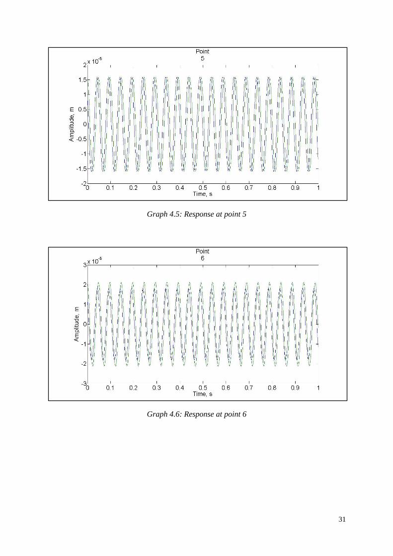
15 graphs are then generated from MATLAB to compare the graphs plotted by using the
response from the ODS data and the response calculated from modal analysis. The generated
graphs are shown as follows with the green line representing the graph generated from ODS
and the blue line representing the graph generated from response calculated by using the data
obtained from modal analysis.
Graph 4.1: Response at point 1
Graph 4.2: Response at point 2
Page 33
30
Graph 4.3: Response at point 3
Graph 4.4: Response at point 4
Page 34
31
Graph 4.5: Response at point 5
Graph 4.6: Response at point 6
Page 35
32
Graph 4.7: Response at point 7
Graph 4.8: Response at point 8
Page 36
33
Graph 4.9: Response at point 9
Graph 4.10: Response at point 10
Page 37
34
Graph 4.11: Response at point 11
Graph 4.12: Response at point 12
Page 38
35
Graph 4.13: Response at point 13
Graph 4.14: Response at point 14
Page 39
36
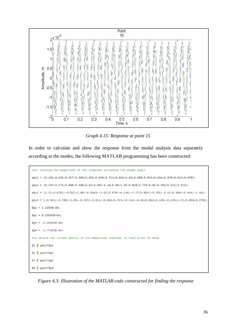
Graph 4.15: Response at point 15
In order to calculate and show the response from the modal analysis data separately
according to the modes, the following MATLAB programming has been constructed:
Figure 4.3: Illustration of the MATLAB code constructed for finding the response
Page 40
37
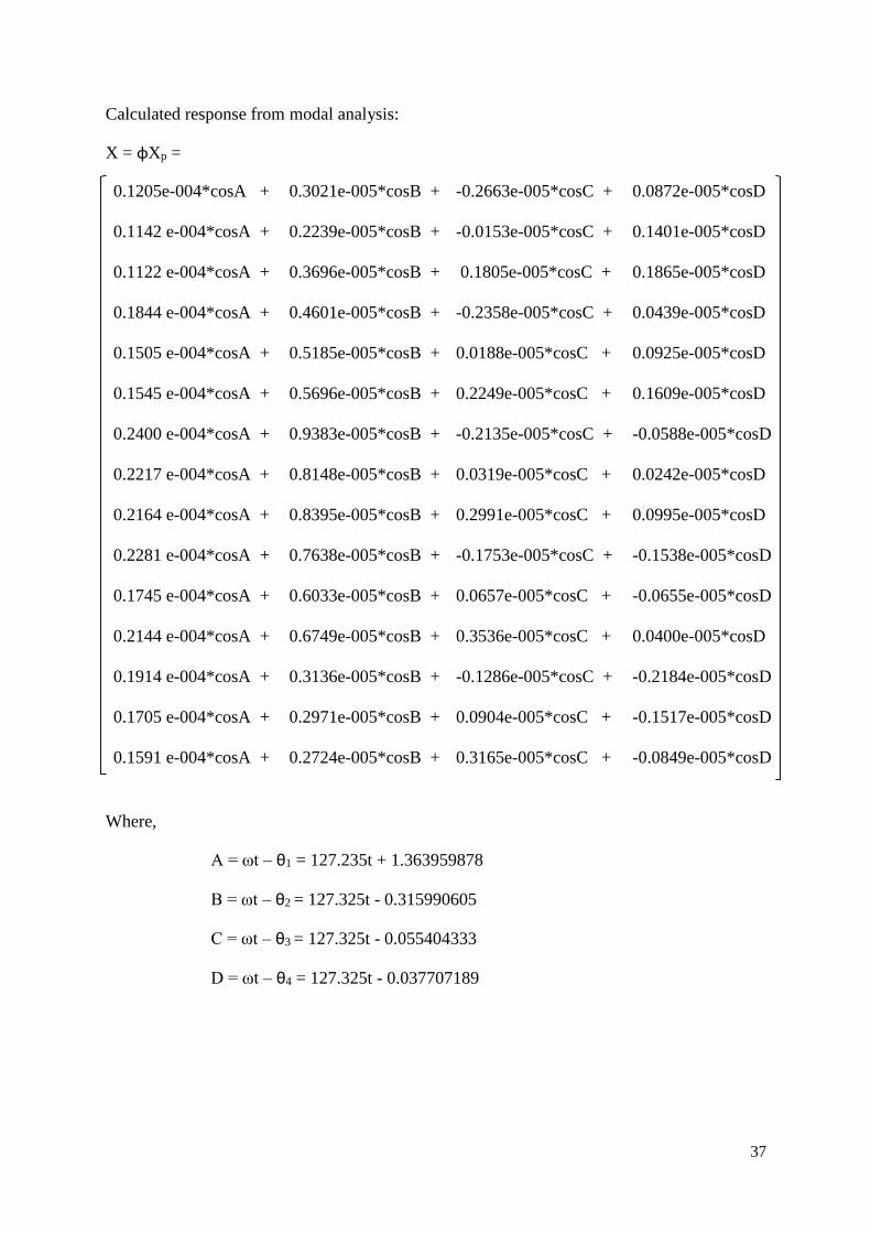
Calculated response from modal analysis:
X = φXp =
0.1205e-004*cosA + 0.3021e-005*cosB + -0.2663e-005*cosC + 0.0872e-005*cosD
0.1142 e-004*cosA + 0.2239e-005*cosB + -0.0153e-005*cosC + 0.1401e-005*cosD
0.1122 e-004*cosA + 0.3696e-005*cosB + 0.1805e-005*cosC + 0.1865e-005*cosD
0.1844 e-004*cosA + 0.4601e-005*cosB + -0.2358e-005*cosC + 0.0439e-005*cosD
0.1505 e-004*cosA + 0.5185e-005*cosB + 0.0188e-005*cosC + 0.0925e-005*cosD
0.1545 e-004*cosA + 0.5696e-005*cosB + 0.2249e-005*cosC + 0.1609e-005*cosD
0.2400 e-004*cosA + 0.9383e-005*cosB + -0.2135e-005*cosC + -0.0588e-005*cosD
0.2217 e-004*cosA + 0.8148e-005*cosB + 0.0319e-005*cosC + 0.0242e-005*cosD
0.2164 e-004*cosA + 0.8395e-005*cosB + 0.2991e-005*cosC + 0.0995e-005*cosD
0.2281 e-004*cosA + 0.7638e-005*cosB + -0.1753e-005*cosC + -0.1538e-005*cosD
0.1745 e-004*cosA + 0.6033e-005*cosB + 0.0657e-005*cosC + -0.0655e-005*cosD
0.2144 e-004*cosA + 0.6749e-005*cosB + 0.3536e-005*cosC + 0.0400e-005*cosD
0.1914 e-004*cosA + 0.3136e-005*cosB + -0.1286e-005*cosC + -0.2184e-005*cosD
0.1705 e-004*cosA + 0.2971e-005*cosB + 0.0904e-005*cosC + -0.1517e-005*cosD
0.1591 e-004*cosA + 0.2724e-005*cosB + 0.3165e-005*cosC + -0.0849e-005*cosD
Where,
A = ωt – θ1 = 127.235t + 1.363959878
B = ωt – θ2 = 127.325t - 0.315990605
C = ωt – θ3 = 127.325t - 0.055404333
D = ωt – θ4 = 127.325t - 0.037707189
Page 41
38
4.2 Discussion
The dynamic behaviour of machine structures depends on the following factors:
i. The closeness of excitation frequency to the natural frequency
ii. The relationship between excitation force distribution and mode shape
iii. The amount of damping in the structure
The natural frequency, mode shape and damping formed the 3 dynamic characteristics of
the system whereas material properties, boundary condition and geometry are the elements that
contribute to different mode shape and damped frequency.
The screenshot obtained from the modal analysis showing the vibration response at mode
1 are illustrated in the figure as follows:
Figure 4.4: Illustration of vibration response at 20 Hz (mode shape 1)
From the figure, the damped natural frequency of this mode is observed to be 20 Hz.
Every points in this mode are in almost similar phase. Highest eigenvector magnitude is
observed at point 7 with a magnitude of 0.721 m/N-sec.
Page 42
39
The screenshot obtained from the modal analysis showing the vibration response at
mode 2 are illustrated in the figure as follows:
Figure 4.5: Illustration of vibration response at 25.1 Hz (mode shape 2)
From the figure, the damped natural frequency of this mode is observed to be 25.1 Hz.
Every points in this mode are in almost similar phase. Highest eigenvector magnitude is
observed at point 7 with a magnitude of 1.14 m/N-sec.
The screenshot obtained from the modal analysis showing the vibration response at
mode 3 are illustrated in the figure that follows (see Figure 4.6). Damped frequency of this
mode is observed to be 45.1 Hz. The graph shown point 3, point 6, point 9, point 12 and point
15 are at the similar phase but are out of phase with point 1, point 4, point 7, point 10 and point
13. There is very little or no deflection at point 2, point 5, point 8, point 11 and point 14. This
is because these points are the nodal points at this mode. Highest magnitude is observed at
point 12 with a magnitude of 1.62 m/N-sec.
Page 43
40
Figure 4.6: Illustration of vibration response at 45.1 Hz (mode shape 3)
The screenshot obtained from the modal analysis showing the vibration response at
mode 4 are illustrated in the figure that follows (see Figure 4.7).
Figure 4.7: Illustration of vibration response at 54.3 Hz (mode shape 4)
Page 44
41
The damped natural frequency of this mode is observed to be 54.3 Hz. The graph has
shown that point 1, point 2, point 3, point 4, point 5, and point 6 at the similar phase but are
out of phase with point 10, point 11, point 12, point 13, point 14 and point 15. There is very
little or no deflection at point 7, point 8 and point 9. This is because they act as the nodal points
at this mode. Highest magnitude is observed at point 13 with magnitude of 1.23 m/N-sec.
The screenshot obtained from the Operational Deflection Shape (ODS) showing the
vibration response at an excitation frequency of 20.25 Hz are illustrated in the figure that
follows:
Figure 4.7: Illustration of vibration response at an excitation force of 20.25 Hz
The mode shape obtained from ODS (Operation deflection shape) is shown in figure
4.7. It is observed to be similar to mode shape 1 as illustrated in figure 4.4. This can be
explained by the first factor that determines the dynamic behavior of a structure as mentioned
earlier which is the closeness of excitation frequency to the natural frequency.
Since the excitation frequency of the force is 20.25 Hz, it is very close to the damped
natural frequency and natural frequency of Mode shape 1 that are 20 Hz and 20.03 Hz
Page 45
42
respectively. Since their frequencies are very close to each other, the structure will thus vibrate
in a similar manner.
Apart from that, from the calculation by using the data from modal analysis, the
response of the structure in matrix form, X = φXp, which is determined earlier from the
calculation in section 4.1 is found to be contributed the most by mode 1. As we can see from
the matrix X, when the response contributed by each mode are all added together in each point,
it is found that the response in mode 1 constitutes a larger amount in magnitude compared to 3
other modes. This can also be explained by the first factor that affect the dynamic behavior of
the structure which is the closeness of excitation frequency, which in this case 20.25 Hz to the
natural frequency which in this case, the damped natural frequency and natural frequency of
mode 1 that are 20 Hz and 20.03 Hz respectively.
According to figure 4.1 to 4.15, comparing the result of ODS and harmonic response,
all of the graph are in same phase and match nicely together. This result shows that the
excitation force is identical to the natural frequency of the structure and hence resonance occur.
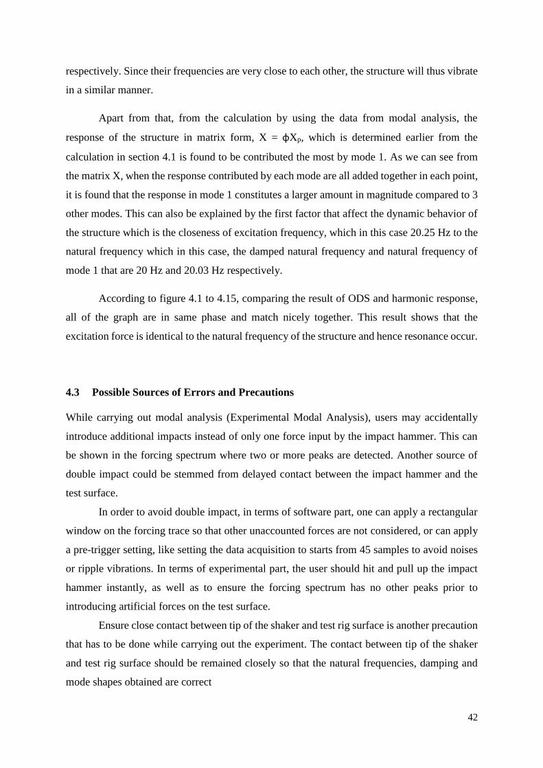
4.3 Possible Sources of Errors and Precautions
While carrying out modal analysis (Experimental Modal Analysis), users may accidentally
introduce additional impacts instead of only one force input by the impact hammer. This can
be shown in the forcing spectrum where two or more peaks are detected. Another source of
double impact could be stemmed from delayed contact between the impact hammer and the
test surface.
In order to avoid double impact, in terms of software part, one can apply a rectangular
window on the forcing trace so that other unaccounted forces are not considered, or can apply
a pre-trigger setting, like setting the data acquisition to starts from 45 samples to avoid noises
or ripple vibrations. In terms of experimental part, the user should hit and pull up the impact
hammer instantly, as well as to ensure the forcing spectrum has no other peaks prior to
introducing artificial forces on the test surface.
Ensure close contact between tip of the shaker and test rig surface is another precaution
that has to be done while carrying out the experiment. The contact between tip of the shaker
and test rig surface should be remained closely so that the natural frequencies, damping and
mode shapes obtained are correct
Page 46
43
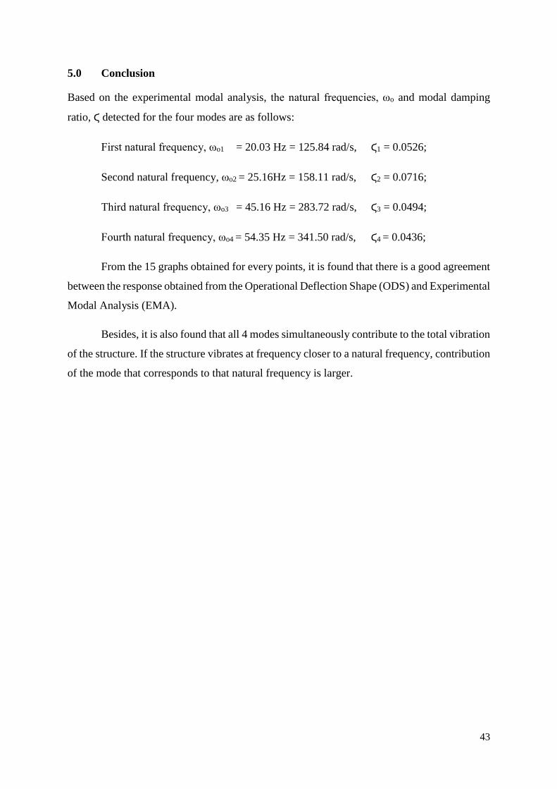
5.0 Conclusion
Based on the experimental modal analysis, the natural frequencies, ωo and modal damping
ratio, Ϛ detected for the four modes are as follows:
First natural frequency, ωo1 = 20.03 Hz = 125.84 rad/s, Ϛ1 = 0.0526;
Second natural frequency, ωo2 = 25.16Hz = 158.11 rad/s, Ϛ2 = 0.0716;
Third natural frequency, ωo3 = 45.16 Hz = 283.72 rad/s, Ϛ3 = 0.0494;
Fourth natural frequency, ωo4 = 54.35 Hz = 341.50 rad/s, Ϛ4 = 0.0436;
From the 15 graphs obtained for every points, it is found that there is a good agreement
between the response obtained from the Operational Deflection Shape (ODS) and Experimental
Modal Analysis (EMA).
Besides, it is also found that all 4 modes simultaneously contribute to the total vibration
of the structure. If the structure vibrates at frequency closer to a natural frequency, contribution
of the mode that corresponds to that natural frequency is larger.