IN DEGREE PROJECT MEDICAL ENGINEERING, SECOND CYCLE, 30 CREDITS , STOCKHOLM SWEDEN 2018 Knowledge Discovery and Data mining using demographic and clinical data to diagnose heart disease. JAVIER FERNÁNDEZ SÁNCHEZ KTH ROYAL INSTITUTE OF TECHNOLOGY SCHOOL OF ENGINEERING SCIENCES IN CHEMISTRY, BIOTECHNOLOGY AND HEALTH
Transcript
IN DEGREE PROJECT MEDICAL ENGINEERING,SECOND CYCLE, 30 CREDITS
, STOCKHOLM SWEDEN 2018
Knowledge Discovery and Data mining using demographic and clinical data to diagnose heart disease.
JAVIER FERNÁNDEZ SÁNCHEZ
KTH ROYAL INSTITUTE OF TECHNOLOGYSCHOOL OF ENGINEERING SCIENCES IN CHEMISTRY, BIOTECHNOLOGY AND HEALTH
i
Abstract
Cardiovascular disease (CVD) is the leading cause of morbidity, mortality, premature death and reduced quality
of life for the citizens of the EU. It has been reported that CVD represents a major economic load on health care sys-
tems in terms of hospitalizations, rehabilitation services, physician visits and medication. Data Mining techniques
with clinical data has become an interesting tool to prevent, diagnose or treat CVD. In this thesis, Knowledge Dis-
covery and Data Mining (KDD) was employed to analyse clinical and demographic data, which could be used to
diagnose coronary artery disease (CAD). The exploratory data analysis (EDA) showed that female patients at an el-
derly age with a higher level of cholesterol, maximum achieved heart rate and ST-depression are more prone to be
diagnosed with heart disease. Furthermore, patients with atypical angina are more likely to be at an elderly age with
a slightly higher level of cholesterol and maximum achieved heart rate than asymptotic chest pain patients. More-
over, patients with exercise induced angina contained lower values of maximum achieved heart rate than those
who do not experience it. We could verify that patients who experience exercise induced angina and asymptomatic
chest pain are more likely to be diagnosed with heart disease. On the other hand, Logistic Regression, K-Nearest
Neighbors, Support Vector Machines, Decision Tree, Bagging and Boosting methods were evaluated by adopting
a stratified 10 fold cross-validation approach. The learning models provided an average of 78-83% F-score and a
mean AUC of 85-88%. Among all the models, the highest score is given by Radial Basis Function Kernel Support
Vector Machines (RBF-SVM), achieving 82.5% ± 4.7% of F-score and an AUC of 87.6% ± 5.8%. Our research con-
firmed that data mining techniques can support physicians in their interpretations of heart disease diagnosis in
addition to clinical and demographic characteristics of patients.
ii
Aknowledgements
First, I would like to thank BYON8 AB for giving the opportunity to let me be involved in an amazing and pas-
sionate world of a health-tech start-up. I would like to reserve particular gratification to Matias and Josef for their
support and guidance through these intensive months.
Thanks to all my classmates who became friends, with a special thanks to Jakob who made my days a bit easier
here in the north by eating tortillas every weekend.
Special thanks to my colleagues who have supported me during this journey and to Kassim Caratella who is still
the best international manager superstar.
Another special thanks for my previous supervisor and friend Inma from Universidad Rey Juan Carlos (URJC)
who provided me support and advice with regular meetings.
Last but not least, my very special thanks to my mother who is always there no matter what. Thanks also to the
rest of my family (sister, father and Mario) who support me every day in this adventure in the North. THANKS.
iii
“If you have an apple and I have an apple and we exchange these apples
then you and I will still each have one apple. But if you have an idea
and I have an idea and we exchange these ideas, then each of us will have two ideas"
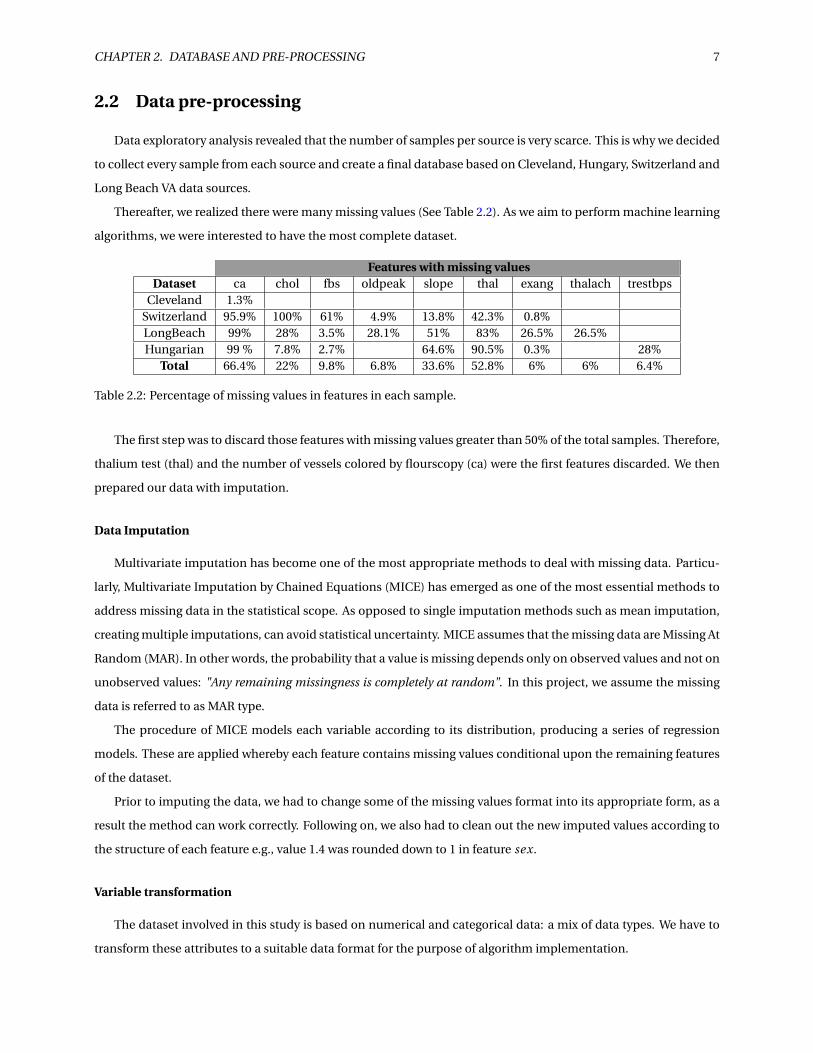
We can distinguish between two types of categorical data: nominal and ordinal. The first type does not have
any sense of order among discrete categorical values, while it does for ordinal data.
In our dataset, we just have nominal data since there is no notion of order among the categorical values in any
feature.
The idea here is to transform the categorical features into a more representative numerical format which can
be understood by the machine learning algorithms. Thus, first the categorical values should be transformed into
numerical labels and then applying some encoding scheme to these values.
Considering we have the numeric representation of any categorical attribute with m labels, the OHE scheme,
encodes the feature into m binary attributes which can only contain a value of 0 (absence) or 1 (presence). For
CHAPTER 2. DATABASE AND PRE-PROCESSING 9
instance, if we have a categorical feature named chest pain type which contains 4 values: typical angina, atypical
angina, non-anginal pain and asymptomatic. The first step will be to transform these values into numeric repre-
sentation, and then generating 4 new features which would be cp1, cp2, cp3 and cp4 containing only 0 and 1 values
in each new feature.
Feature selection
In several practical data mining situations, there are many attributes or features to be handled and most of them
are clearly redundant or irrelevant. Many machine learning techniques try to select the most appropriate features,
but this often leads to model performance deterioration.
This can be improved by discarding those irrelevant attributes and keep the ones the models actually use. The
advantages of feature selection are many. Reducing dimensionality speeds up the computation of those algorithms
as well as providing a more compact and easy interpretable representation of the target. Moreover, it also reduces
the problem of overfitting, where a learned machine learning model is tied up too closely to the training data.
Therefore, it outperforms better on training data than on new unseen instances.
In this study, we tried several feature selection approaches along with machine learning techniques to identify
the most relevant attributes of the dataset.
Attribute clustering can be useful for creating models. It allows analysts to see the relationship of these at-
tributes and a particular extent of choice. The idea behind hierarchical clustering is pretty simple: initially each
attribute is considered as its own cluster. The algorithm then finds the two closest clusters in terms of distance or
similarity measure, merge them and continues doing this until there is just one cluster left.
Figure 2.2 shows a bottom-up approach hierarchical clustering that recursively merges features following the
same basis as described previously. It uses the single linkage criterion which determines the distance (correlation)
to use between sets of attributes.
We can observe that some of the features are correlated with each other: (cp4 - exang1), (exang0 - thal ach)
and (exang1 - ol d peak) are one of the set of attributes with strongest correlation with each other.
CHAPTER 2. DATABASE AND PRE-PROCESSING 10
Figure 2.2: Dendrogram of the resulting cluster hierarchy (agglomerative) which has chosen the most relevantattributes. The heatmap shows the extent of correlation between features.
Furthermore, we also used Recursive Feature Elimination (RFE). The procedure works as follows: an external
estimator (a machine learning scheme) assigns weights to features e.g., the coefficients in a linear model, then
it selects those features by recursively considering smaller sets of features. Thus, first the estimator is trained and
then it selects those features with more importance and discard those irrelevant attributes from the set. It continues
until the desired number of features is eventually reached.
Due to the imbalance of our dataset, we perform this algorithm with 10-fold stratified cross validation. We used
two estimators, a support-vector machine (SVM) scheme with linear kernel and a random forest (RF) estimator.
CHAPTER 2. DATABASE AND PRE-PROCESSING 11
(a) (b)
Figure 2.3: Mean accuracy of a RFE 10-fold stratified cross validation approach considering different number offeatures using (a) Random Forest and (b) Support vector machines (linear kernel).
According to Figure 2.3, we can claim that the number of features selected with RF as estimator, which gives
the best score, is 10. ag e, sex0, cp2, cp4, tr estbps, chol , r estecg0, thal ach, exang0 and ol d peak. On the other
hand, SVM-linear estimator provides 17 features selected which provide the best cross-validation score. However,
we can see there is a peak when the number of features selected is ten which gives a slightly lower score than the
best. These 10 features are: sex0, sex1, cp2, cp4, chol , f bs0, thal ach, exang0, exang1, ol d peak.
We also applied tree-based methods to evaluate the importance in a classification task. Importance in this
context is often called "Gini Importance" or "Mean Decrease Impurity" and it is defined as the total decrease in
node impurity, weighted by the probability of reaching that particular node, which is approximated by the number
of samples reaching that node. Then it is averaged over all trees of the ensemble [4].
(a) (b)
Figure 2.4: Feature ranking using (a) Extra Trees and (b) Random Forest along with their inter-trees variability.
In addition to Random Forest, the other estimator considered in this case is: Extremely randomized trees, which
is a meta estimator which fits a number of randomized decision trees on the training data and use averaging to
improve the predictive accuracy and control overfitting.
CHAPTER 2. DATABASE AND PRE-PROCESSING 12
According to Figure 2.4, we can see that the most relevant features for both estimators are chol , thal ach, ag e,
cp4, ol d peak, tr estbps, exang0 and exang1 then the rest contains very little importance and becomes constant
for the remaining features.
Considering all of these methods which gives different results, we tried selecting different features and verified
the best performance is given by discarding the following features: sl ope1,2,3, f bs0,1, cp1,3 and r estecg0,1,2.
Hence the final dataset contains, in addition to the target feature hear tdi sease, the following: ag e, sex0,1,
cp2,4, tr estbps, chol , thal ach, exang0,1 and ol d peak.
Chapter 3
Exploratory Data Analysis
An exploratory analysis is an essential step towards performing high quality research. This step of the study has
been performed along with the data pre-processing. It was essential to verify how the missing data was distributed
and what approach was better to address. Moreover, it was also useful to see how similar are some feature distribu-
tions with each other. Section 3.1 of this chapter refers to how numerical features are distributed across different
values of categorical data. Later in Section 3.2, we showed the distribution of each sample in each numerical feature
across different categories of categorical features.
We resolved that cp1,3 (typical angina and non-anginal pain) were discarded according from our feature selec-
tion algorithms. According to the figures illustrated in this Chapter (See sub-figures in Figure 3.1 and Figure 3.2).
This was done due to the limited amount of available samples from this level in chest pain feature (See middle
column subfigures in Figure 3.2)
3.1 Violin plots of relevant features
In this section we showed the distribution of quantitative data (age, cholesterol, maximum heart rate achieved,
resting blood pressure and ST Depression induced by exercise relative to rest) across different levels of the sex,
chest pain type and exercise induced angina features. Each subfigure illustrated a kernel density estimation (KDE)
of the underlying distribution of each level in each categorical feature, making a clear distinction of diagnosing
heart disease. The dotted lines describes the median (middle line) and the quartiles (both sides). Note that KDE is
influenced by the sample size and features with relatively small samples might look misleadingly smooth. Also, we
determined some outliers (thin line at the tails of each violin).
According to each subfigure in Figure 3.1 we can claim that female patients are diagnosed with heart disease
at an elderly age, higher level of cholesterol, maximum heart rate achieved and ST depression than male patients.
Female patients accounted for 21.1% of the population considered in the dataset while male patients proportion is
89.9% (See Table 2.1b).
Chest pain type could give us a good idea about which patients are diagnosed with heart disease, in particu-
13
CHAPTER 3. EXPLORATORY DATA ANALYSIS 14
lar, those patients with atypical angina or it asymptomatic. We discovered that asymptomatic patients suffer heart
disease at a similar elderly age than atypical angina but the latter one is more likely to be at an elderly age; pa-
tients with atypical angina are diagnosed heart disease at a bit higher cholesterol levels and maximum heart rate
achieved than patients with no symptoms in their chest; atypical angina contains similar resting blood pressure to
asymptomatic patients, but the distribution is slightly skewed to higher values. On the other hand, we determined
that there are some outliers in asymptomatic patients and that atypical angina distribution is much more smoother
than asymptomatic patients.
Furthermore, we concluded that the maximum heart rate for patients with exercise angina is lower than for
those ones who do not experience it. Younger patients are more prone to suffer exercise induced angina.
3.2 Scatter plots of relevant features
Showing each observation at each level of the categorical variable is also very useful to check which features are
more discriminatory to diagnose heart disease and also to check if there are enough samples in each feature to take
it into consideration for our models. Before feature selection, we revealed the discarded attributes have very scarce
observations.
According to Figure 3.2, we could state that male patients have a quite good extent of discrimination of heart
disease. In addition to this, we determined that asymptomatic chest pain patients are more prone to be diagnosed
with heart disease. Moreover, patients who experienced exercise induced angina are also prone to suffer heart
disease. We concluded that the discarded features e.g., typical angina does not contain many observations. On
the other hand, features with not so many observations e.g, female patients showed a much smoother feature
distribution as expected.
CHAPTER 3. EXPLORATORY DATA ANALYSIS 15
(a) (b) (c)
(d) (e) (f)
(g) (h) (i)
(j) (k) (l)
(m) (n) (o)
Figure 3.1: Distribution of (a), (b) and (c) age; (d), (e) and (f) cholesterol; (g), (h) and (i) maximum heart rate achieved, (j),(k) and (l) resting blood pressure; (m), (n) and (o) ST-depression induced by exercise relative to rest across sex (leftcolumn), chest pain type (middle column) and exercise induced angina (right column).
CHAPTER 3. EXPLORATORY DATA ANALYSIS 16
(a)(b)
(c)
(d)(e)
(f)
(g)(h)
(i)
(j)(k)
(l)
(m)(n)
(o)
Figure 3.2: Sample distribution of (a), (b) and (c) age; (d), (e) and (f) cholesterol; (g), (h) and (i) maximum heart rateachieved, (j), (k) and (l) resting blood pressure; (m), (n) and (o) ST-depression induced by exercise relative to rest acrosssex (right column), chest pain type (middle column) and exercise induced angina (left column).
Chapter 4
Machine Learning approaches and
parameter tuning
In this Chapter we presented the learning algorithms used in the project. We adopted a 10-fold cross-validation
approach along with random search to find the set of parameters which optimize the learning algorithms. In Sec-
tion 4.1 we described the approaches for tuning hyper-parameters. Later in Section 4.2 and Section 4.3, hyper-
parameters from single and ensemble machine learning algorithms are illustrated.
4.1 Tuning parameters
A typical learning algorithm A aims to find a function f that minimizes some expected Loss(x; f ) over i.i.d x
samples from a distribution Gx . These learning algorithms usually produce f through optimization of a training
principle regarding a set of parameters θ. Despite this, the learning algorithm is obtained by choosing some hyper-
parameters λ. For example, with a Linear kernel SVM, one should select an appropriate regularization parameter
C for this training principle [5].
Hyper-parameter optimization is the name for selecting the best hyper-parameters that provides the best learn-
ing performance. Grid search and manual search are the most widely used strategies. However, this performs too
many trials and yields prohibitively expensive in computing cost terms. Furthermore, it is also proved for most of
datasets, only a few of the hyper-parameters really matter. Random search paves these issues as not all the hyper-
parameters are equally relevant and on the top of that, it gives same or better performance than grid search in less
computational time [5].
Therefore, tuning a model is where machine learning turns from a science into trial-and-error based engineer-
ing which can be accomplished by Random Search.
17
CHAPTER 4. MACHINE LEARNING APPROACHES AND PARAMETER TUNING 18
4.2 Single methods
In this section, we state the range of parameters used and the best set of parameters for every single method
considered.
Logistic Regression
Parameters Grid Best valuePenalty [l1, l2] l2
C [10−5, 10−4, 10−3,..., 104, 105] 10−2
Table 4.1: Grid of searching parameters for a Logistic Regression Model and its best values found via randomsearch with 10-cross validation strategy. The Parameters are: Penalization and the inverse of regularizationstrength (C ).
K-Nearest Neighbors (KNN)
Parameters Grid Best value#Neighbors [1, 100] 22
Table 4.2: Grid of searching parameters for a KNN model. The parameter tuned is the number of neighbors.
Radial Basis Function (RBF) kernel - Support Vector Machines (RBF-SVM)
Table 4.3: Grid of searching parameters for a Linear-SVM model. The parameters used are: C which trades offmisclassification of training examples against simplicity of the decision surface. A low C makes the decisionsurface smooth, while a high C aims at classifying all training examples correctly; γ defines how much influence asingle training example has. The larger γ is, the closer other examples must be to be affected. Moreover, its bestvalues found via random search with 10-cross validation strategy are stated.
Linear kernel- Support Vector Machines (Linear-SVM)
Parameters Grid Best valueC [10−5, 10−4, 10−3,..., 104, 105] 0.1
Table 4.4: Grid of searching parameters for a Linear-SVM model. The parameters used are: C which trades offmisclassification of training examples against simplicity of the decision surface. A low C makes the decisionsurface smooth, while a high C aims at classifying all training examples correctly. Moreover, its best values foundvia random search with 10-cross validation strategy are stated.
CHAPTER 4. MACHINE LEARNING APPROACHES AND PARAMETER TUNING 19
Decision Trees
Parameters Grid Best valuecriterion to split [gini, entropy] gini
maximum depth of the tree [None, 2, 5, 10] 2minimum #samples required
to split an internal node[2, 10, 20] 2
minimum #samples requiredto be at a leaf node
[1, 5, 10] 10
maximum #leaf nodes [None, 5, 10, 20] 10
Table 4.5: Grid of searching parameters for a Decision Tree and its best values found via random search with10-cross validation strategy.
4.3 Ensemble methods
Here, we present the different range of values for parameters used in different ensemble methods.
4.3.1 Voting classifiers
Voting classifier combines different learning algorithms and use argmax of the sum of predicted probabilities
of the classes/targets weighted. This is called soft voting or weighted average probabilities. We used this ensemble
method with all the previous algorithms illustrated in Section 4.2. The parameters used in the base estimators of
the voting classifier are those ones found via random search.
4.3.2 Bootstrap aggregating (Bagging)
These methods build several instances of a black-box algorithm on random subsets of the original training set
and then aggregate their individual predictions to form a final prediction. In this ensemble algorithm the variance
of a base estimator such as a decision tree is reduced by introducing randomization. Additionally, they provide
a way to reduce overfitting. In theory, bagging methods works best with complex and strong techniques. In this
case, we built bagging algorithms from the single methods considered in Section 4.2. The parameters tuned in this
ensemble method are the number of base estimators in the ensemble.
Base estimator Parameters Grid Best valueLogistic Regression #estimators [100, 1000] 300
Table 4.8: Grid of searching parameters for AdaBoost methods considering logistic regression and decision trees asthe weak learners. Moreover, its best values found via random search with 10-cross validation strategy are stated.
4.3.6 Gradient Tree Boosting Classifier (GTB)
Gradient boosting builds a sequence of functions fk (x), which quality is increased step by step. The quality is
often viewed in terms of a mean square error metric (y − f (x))2 where y is the predicted variable. At each step k, a
small function hk is built in order to to improve the previous approximation fk−1 = h1 + ·· ·+hk−1 approximating
the residual from the previous step, i.e., hk solves the problem argminh((y − fk−1 −h)2).
Table 4.9: Grid of searching parameters for Gradient Tree Boosting method. Moreover, its best values found viarandom search with 10-cross validation strategy are stated. Subsample denotes the fraction of observations to berandomly samples for each tree.
Table 4.10: Grid of searching parameters for XGB method considering logistic regression and decision trees as theweak learners. Moreover, its best values found via random search with 10-cross validation strategy are stated.Lambda (L2 regularization term on weights) and α (L1 regularization term on weigh) are the regularizationparameters; subsample denotes the fraction of observations to be randomly samples for each tree; γ specifies theminimum loss reduction required to make a split; column sample by trees denotes the fraction of columns to berandomly samples for each tree.
Chapter 5
Results and discussion
In this chapter, we analyzed the results obtained by applying the techniques previously discussed. First, we
showed the most relevant evaluation metrics by adopting a stratified 10-fold cross validation approach. Finally, we
compared the results captured in this study with previous research.
5.1 Model validation
Model performance measures are shown in this section. The results are obtained using our final pre-processed
database including cleaning, feature selection and variable transformation presented in Chapter 2. Since the
database is imbalanced, the variable of highest importance for evaluation was deemed to be the F-score (as it fac-
tors in both sensitivity and precision), in addition to AUC (as it factors in both True Positive rate and False Positive
Rate). Therefore, we will discuss the F-score and AUC obtained in relation to training and test data.
First, we focus on single methods (See Table 5.1 and Figure 5.2): regarding test data, we can see that RBF-SVM
provides the highest F-score 82.5%±4.7%, while K-NN method gives 0.1% lower score. However we revealed that
K-NN gives 84.6%±0.6% of training F-score: a bit higher in comparison to RBF-SVM. Hence, the generalization is
better achieved in RBF-SVM. Moreover, we determined that 50% of the folds are higher than 82% and that 25% of
the F-scores falls within the range 85% and 9̃0% F-score (See Figure 5.2 -b). On the other hand, Decision Tree is the
worst model in terms of F-score.
The AUC reveal more information about what is the best model. According Table 5.6a and Figure 5.6, we found
that the highest AUC is given by RBF-SVM (87.6%), whereas Decision Tree provides the lowest AUC (86%).
23
CHAPTER 5. RESULTS AND DISCUSSION 24
(a) (b)
Figure 5.1: Boxplots for (a) training and (b) testing data of single learning algorithms using a stratified 10-foldcross a validation approach.
Regarding Bagging algorithms, we concluded that the mean F-score of Linear-SVM and Decision Tree has im-
proved 0.3% and 0.4% in relation to single methods, respectively; whereas the rest of learning algorithms remained
equal or slightly worse (See Table 5.2. Furthermore, we see the training accuracy has decreased 0.1-0.3%, meaning
the generalization improved.
On the other hand, the mean AUC improved in every case: Linear-SVM and RBF-SVM around 0.2%, Logistic
Regression and KNN around 0.1% and Decision Tree around 1.1% (See Table 5.6a and Figure 5.6).
(a) (b)
Figure 5.2: Boxplots for (a) training and (b) testing data of bagging methods applying the previous learningalgorithms as based estimators and using a stratified 10-fold cross a validation approach.
Improvement in Decision Tree classifier led us to further investigate tree-based methods. We tried different
ensemble learning methods to see how far it could be enhanced. We found that Random Forest achieved 81.7%
F-score on test data, which is 1.4% higher than a single decision tree. Conversely, Extremely Randomized Trees
and Random Forest provided 81.6% F-score on test data. However, we determined that generalization in Random
Forest is not achieved since the results in training data outperforms test data (See Figure 5.3a, Table 5.3 and Figure
5.3).
CHAPTER 5. RESULTS AND DISCUSSION 25
(a) (b)
Figure 5.3: Boxplots for (a) training and (b) testing data of tree-based learning algorithms using a stratified 10-foldcross a validation approach.
With regard to the AUC, it has improved around 1% in Random Forest and bagging trees, while Extremely Ran-
domized Trees goes further to 1.2% improvement regarding single decision trees (See Table 5.3 and Figure 5.7a).
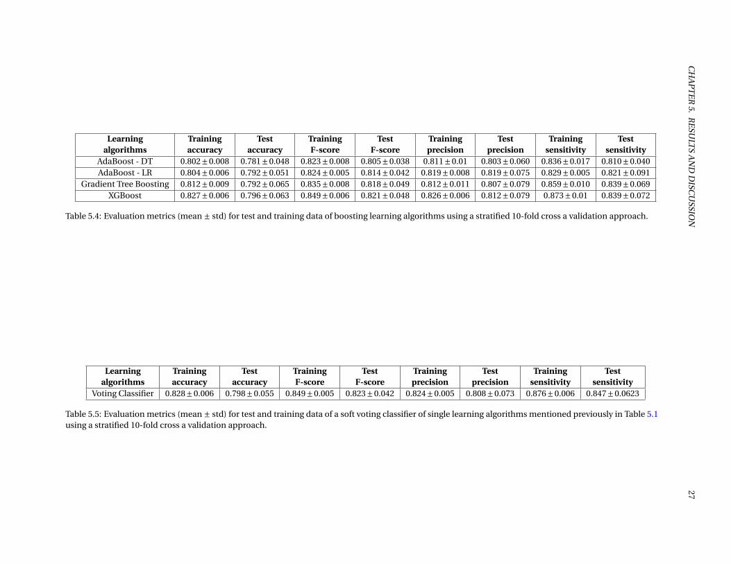
Furthermore, we evaluated boosting methods, which decreases bias of the learning algorithms. We could ver-
ify that the XGBoost provides the best performance (82.1% mean F-score on test data) along with AdaBoost with
logistic regression as a weak learner. On the other hand, we concluded that these learning algorithms generalizes
less than the rest, since the F-score for training data is relatively higher than test data. (See Table 5.4 and see Figure
5.4). Regarding AUC, Voting Classifier shows the highest value along with XGBoost and Gradient Tree Boosting.
(a) (b)
Figure 5.4: Boxplots for (a) training and (b) testing data of Boosting methods and Voting classifier using a stratified10-fold cross a validation approach.
To conclude, we can claim almost all the classifiers considered in this project provide similar mean F-score
results. Random Forest presented a relatively high training mean F-score on test data, even though we tuned the
hyper-parameters. Nevertheless, SVM-RBF yields the best results in terms of mean F-score in relation to test and
Decision Tree 0.782±0.007 0.763±0.051 0.806±0.008 0.789±0.048 0.797±0.025 0.782±0.061 0.817±0.042 0.802±0.075
Table 5.1: Evaluation metrics (mean ± std) for test and training data of single learning algorithms using a stratified 10-fold cross a validation approach.
Decision Tree 0.790±0.007 0.770±0.050 0.811±0.006 0.793±0.047 0.810±0.01 0.797±0.061 0.812±0.013 0.841±0.080
Table 5.2: Evaluation metrics (mean ± std) for test and training data of bagging methods applying the previous learning algorithms as based estimators andusing a stratified 10-fold cross validation approach.
Learningalgorithms
Trainingaccuracy
Testaccuracy
TrainingF-score
TestF-score
Trainingprecision
Testprecision
Trainingsensitivity
Testsensitivity
Random Forest 0.895±0.005 0.799±0.054 0.908±0.041 0.817±0.047 0.881±0.005 0.803±0.072 0.938±0.006 0.841±0.081Extremely
Table 5.3: Evaluation metrics (mean ± std) for test and training data of ensemble tree-based learning algorithms using a stratified 10-fold cross a validationapproach.
Table 5.4: Evaluation metrics (mean ± std) for test and training data of boosting learning algorithms using a stratified 10-fold cross a validation approach.
Table 5.5: Evaluation metrics (mean ± std) for test and training data of a soft voting classifier of single learning algorithms mentioned previously in Table 5.1using a stratified 10-fold cross a validation approach.
CHAPTER 5. RESULTS AND DISCUSSION 28
Learningalgorithms
AUC
Linear - SVM 0.875±0.056RBF -SVM 0.876±0.058
Logistic Regression 0.873±0.056K-NN 0.872±0.057
Decision Tree 0.860±0.062
(a)
Learningbase
algorithmsAUC
Linear - SVM 0.877±0.055RBF -SVM 0.878±0.056
Logistic Regression 0.874±0.058K-NN 0.873±0.058
Decision Tree 0.871±0.056
(b)
Table 5.6: Area Under the Curve (AUC) (mean ± std) for test data of (a) single learning algorithms and (b) baggingmethods applying the previous learning algorithms as based estimators using a stratified 10-fold cross a validationapproach.
Learningalgorithms
AUC
Decision Tree 0.854±0.060Random Forest 0.864±0.062
Extremely Randomized Trees 0.866±0.059Bagging Decision Tree 0.864±0.057
(a)
Learningalgorithms
AUC
AdaBoost - DT 0.863±0.0540AdaBoost - LR 0.868±0.0534
Gradient Tree Boosting 0.8705±0.0559XGBoosting 0.8703±0.0561
Voting Classifier 0.8711±0.056
(b)
Table 5.7: Area Under the Curve (AUC) (mean ± std) for test data of (a) decision tree and ensemble tree-basedlearning algorithms and (b) boosting and voting methods applying the previous learning algorithms as basedestimators using a stratified 10-fold cross a validation approach.
(a) (b)
Figure 5.5: ROC for test data of (a) single learning algorithms and (b) bagging methods applying the previouslearning algorithms as based estimators using a stratified 10-fold cross a validation approach.
CHAPTER 5. RESULTS AND DISCUSSION 29
(a) (b)
Figure 5.6: ROC for test data of (a) Tree-based methods and (b) Boosting methods and voting classifier applyingthe previous learning algorithms as based estimators using a stratified 10-fold cross a validation approach.
5.2 Comparison with previous research
Owing to the world-wide increasing mortality of cardiovascular disease each year and the resulting cost require-
ments, many researchers have applied data mining approaches in the diagnosis of heart disease.
In particular, the so-called Cleveland dataset has been used several times due to its powerful information. De-
spite this fact, we have pre-processed the data. In this study, we found many difficulties addressing this stage.
Firstly, the dataset was imbalanced, which is where there are more instances from one class than the other. Sec-
ondly, there is missing data, and thirdly, it contains a mix of data types (categorical and continuous).
The studies found in the literature were very unclear about the pre-processing of the data [10] [11]. A few of
them discarded those instances which contained any single missing sample [12]. Others, just contemplated the
Cleveland data source and discarded the remaining (Hungary, Switzerland, and VA Long Beach). Various research
studies include categorical data with an unclear form of data transformation. On top of that, most of those studies
did not use a cross-validation approach to evaluate their models and they used accuracy instead of F-score as the
most important metric unit. We found one research project [13] which uses a cross-validation strategy, providing
a 48.53% precision with a Naïve Bayes algorithm. Even though this study used cross validation, it used a model
which assumed the features involved are independent from each other. In our view, such assumption cannot be
made due to some features are somewhat correlated and not completely independent from each other.
The highest accuracy was found by Anbarasi, et al [14] with a value of 99.2% using a genetic algorithm with
Decision Tree. However, the study did not use any cross-validation approach nor determined the generalization
nature of the model.
CHAPTER 5. RESULTS AND DISCUSSION 30
This project offers a complete Knowledge Discovery and Data-mining approach, including an exhaustive data
pre-processing, performing MICE imputation and variable transformation with features selection. We then pro-
vided an outright Exploratory Data Analysis, where we showed the distributions of the features. Finally, we tuned
the hyper-parameters and evaluated our models adopting a stratified 10-fold cross-validation approach. The re-
sults are then compared using F-score and AUC due to the imbalanced nature of our dataset, the accuracy metric
was not utilized (see Apendix-A).
Chapter 6
Conclusions and Future Work
In this final chapter, we presented the obtained conclusions. We then illustrated the potential benefits which
can be derived in the health scope. Finally, we described the possible future work which could be developed re-
garding this project topic. As such, we determined how much research remains to be done.
6.1 Conclusions
Nowadays, CAD plays an important role in a clinical and economic context. There is a high percentage of
prevalence among mid-aged people. Furthermore, treatment and control of this particular disease can be expen-
sive. Thus, we aim to provide a tool which can improve the application of available resources regarding this spe-
cific chronic condition. For that purpose, we analyzed demographic and clinical data from the so-called Cleveland
dataset and performed an exhaustive KDD approach which can derive whether a patient suffers heart disease.
Firstly, a pre-processing of this dataset was required due to its inconsistencies. We tried to have the most com-
plete and unbiased dataset. As such, we used MICE imputation. After that, we chose the most important attributes
by means of various feature selection approaches. In addition to the target feature (diagnosis of heart disease), we
extracted the most important attributes using feature engineering. Finally, we transformed these features into a
suitable format that fits the proposed learning algorithms.
Secondly, we performed an exploratory data analysis: the number of male patients is far more higher than
female patients. Furthermore, female patients suffer heart disease at an elderly age, along with a higher level of
cholesterol, maximum heart rate achieved and ST-depression than male patients. Patients with atypical angina are
more likely to be at an elderly age, at a slightly higher level of cholesterol and heart rate achieved than asymptotic
chest pain patients. Moreover, we revealed that those patients with exercise induced angina contains lower values
of maximum heart rate achieved than those who do not experience it.
On the other hand, we could verify that patients who experienced exercise induced angina and asymptomatic
chest pain were more prone to be diagnosed with heart disease.
Eventually, we validated our models adopting a stratified 10-fold cross-validation and showing the ROC, AUC
31
CHAPTER 6. CONCLUSIONS AND FUTURE WORK 32
and mean ± std F-score. We verified that our models (single and ensemble) provide an average of 78-83% F-score
over the folds, and a mean AUC of 85-88%. The highest score is given by Radial Basis Function Kernel Support Vector
Machines (RBF-SVM), achieving 82.5% ± 4.7% and 87.6% ± 5.8% of F-score and AUC, respectively. Conversely, we
found that XGBoost and Random forest did not generalize well (overfitting) as the training F-score is relatively
higher than the test F-score.
In conclusion, we determined that data mining techniques offer other options to physicians to facilitate their
interpretations about diagnosis of heart disease considering clinical and demographic characteristics of patients.
6.2 Future Work
CAD has raised concern due to its relevance as a major cause of death. Statistical analysis and data mining
approaches could support physicians for disease treatment. As such, we present the potential work which remains
to be developed and advanced:
• The dataset dates from the 80’s. Currently, the most relevant characteristics to diagnose heart disease may
have changed since that time. Thus, we propose another study considering current data.
• We had some difficulties applying data-mining techniques to incomplete data. Therefore, another analysis
with only male patients suffering heart disease would be interesting (as those patients had the most complete
information).
• Gathering more data. The number of patients considered in this study (920) does not contain a fair popu-
lation representation. Moreover, those patients presented missing data. A higher number of complete data
examples will add more information to this research and will reduce the generalization problem.
• Performing other ML algorithms such as Neural Networks and some other ensemble methods (Stacking).
• Including data from various geographic location. Probably there are different patterns considering different
data from different places. Diet and lifestyle would differ from one place to another, and thus the character-
istics of patients.
Appendix A
State-of-the-art
In this Appendix, we explained the relevance of cardiovascular diseases, the influence of technology in clinical
decision support and the importance which data is having in real world applications. Later, we described what
some types of Data Mining and Machine Learning techniques which we evaluated in this project. Finally, we illus-
trated the ethics involved using this technique and the evaluation metrics we used to evaluate the performance of
the models involved.
A.1 Cardiovascular Diseases
Cardiovascular diseases (CVD) comprises of a wide range of medical issues of the circulatory system i.e., the
heart, blood vessels and arteries. Some of the most common diseases within this group include ischaemic heart
disease (heart attacks) and cerebrovascular diseases. Even though there is a small reduction of these problems
nowadays, it is still the major cause of death in the EU (See Figure A.1).
People suffering these issues face disability, reduced quality of life and, in some cases, premature death. In-
terventions towards lifestyle aims to reduce the prevalence of these diseases. The amount can be reduced by: the
avoidance of tobacco, at least 30 min/day of physical activity, eating healthy food, avoidance of weight gain and
maintenance of blood pressure below 140/90 mmHg among other factors [3].
In Sweden, CVD is also the major cause of death. Table A.1 shows the length of stay per 100K inhabitants,
the number of admissions per 100K inhabitants, the average length of stay, and the number of patients per 100K
inhabitants. In this table you can see men are more prone to be diagnosed with CVD than women. However,
according to Eurostate, death rates are much higher for women than for men. Moreover, according to Table A.2
the majority of the population aged older than 65 years old contains the highest prevalence of conditions from the
circulatory system.
In recent years, there has been a reduction of the number of deaths related to cardiovascular diseases due to the
discovery and adoption of new technologies such as screening, new ways to undergo surgical procedures as well
as the introduction of medication e.g., statins. There is also a change in the lifestyle of people e.g., less smokers.
33
APPENDIX A. STATE-OF-THE-ART 34
Figure A.1: Causes of death - diseases of the circulatory system in 2014. Extracted from Eurostat [3].
However, it is still the major cause of death and it is taking many lives over the years [3].
Regarding the healthcare personnel, there are between 5 and 20 cardiologist across almost every country from
the EU, with the number increasing every year. This suggests there is a concern about issues with the circulatory
system in the EU [3].
Measure Sex 2013 2014 2015 2016Men 13,882.36 13,528.12 12,817.05 12,105.83
Woman 11,435.02 11,160.15 10,494.56 9,696.34Length of stay per 100,000 inhabitantsBoth sexes 12,656.13 12,342.97 11,656.28 10,903.67
Men 2,674.04 2,583.98 2,486.47 2,385.73Woman 2,003.70 1,924.76 1,845.30 1,728.75Number of admissions per 100,000 inhabitants
Both sexes 2,338.17 2,254.05 2,166.02 2,057.94Men 5.19 5.24 5.15 5.07
Men 1,692.31 1,647.47 1,598.70 1,535.83Woman 1,331.64 1,284.16 1,238.88 1,173.44Number of patients per 100,000 inhabitants
Both sexes 1,511.60 1,465.64 1,418.86 1,355.02
Table A.1: Diagnoses of circulatory system problems in the Swedish In-Patient Care. Age: 0-85+. Statistics taken from The Healthand Welfare Statistical Database of Sweden [15].
APPENDIX A. STATE-OF-THE-ART 35
Measure Sex 2013 2014 2015 2016Men 60,005.52 57,620.33 54,194.81 50,880.36
Woman 46,712.36 45,112.03 41,887.44 38,532.24Length of stay per 100,000 inhabitantsBoth sexes 52,764.85 50,832.97 47,539.05 44,222.65
Men 10,895.95 10,403.94 9,982.16 9,539.22Woman 7,871.80 7,504.07 7,168.67 6,683.24Number of admissions per 100,000 inhabitants
Both sexes 9,248.72 8,830.38 8,460.64 7,999.37Men 5.51 5.54 5.43 5.33
Men 6,864.53 6,601.00 6,386.39 6,105.48Woman 5,206.62 4,976.48 4,786.24 4,524.37Number of patients per 100,000 inhabitants
Both sexes 5,961.48 5,719.49 5,521.03 5,253.00
Table A.2: Diagnoses of circulatory system problems in the Swedish In-Patient Care. Age: 65+. Statistics taken from The Health andWelfare Statistical Database of Sweden [15].
A.2 Clinical Decision Support
Services provided at fast pace are believed to give user’s satisfaction. For example, considering a single medical
appointment: it is claimed a considerable amount of time is wasted when a patient is given "hands-on" treatment
i.e., vital signs, discussing with the physician and undergoing the procedure. Furthermore, there is also wasted
time when the patient is waiting for something to happen. However, healthcare service delivery is a very complex
procedure since each patient has a unique process to go through e.g., physical examination, lab analysis, imaging,
etc. [16] [17] [18].
Increasing quality of care, improving healthcare outcomes, avoiding adverse events or producing mistakes and
improving efficiency, cost-benefit and patient/provider satisfaction involves new ways to address these challenges.
Clinical decision support (CDS) provides assistance to physicians, patients, healthcare providers and related,
improving and enhancing healthcare delivery [19][20]. CDS has been claimed as a very useful tool to improve
healthcare quality [21].
There are mainly four different features to achieve this: i) add decision support to clinician’s plan, ii) bring
decision support at the time and location of the made decision, iii) provide suggestions of actions and iv) using a
computer/electronic device as the means to get decision support [22]. Automatically providing decision support
to physicians, eliminates the time physicians need to spend to look at suggestions of the system.
Furthermore, CDS improves consistency, robustness and reliability by using computers or electronic medical
devices by minimizing costs in terms of time and errors prone to manual entry abstractions. Thus, using CDS is
essential to improve quality-care since it decreases time, initiative and endeavor needed by clinicians to draw and
move towards system recommendations [22].
APPENDIX A. STATE-OF-THE-ART 36
A.2.1 Telehealth
Using electronic services to support clinical decisions such as monitoring, patient-care and education [23]
helps to reduce costs and improve healthcare quality in effective, efficient, timely, safe, equitable and patient-
centered conditions [24][25][26]. To achieve these targets, integration of telehealth into traditional practises should
be accomplished.
Over the last decades, technology innovation has had a great impact in the population improving approaches
to consumers. Think about automated teller machines (ATM), drive-through windows and self-service gas stations
[27] and recently the supermarket with free-checkout which Amazon just released at the beginning of 2018 [28].
Telehealth approaches includes home-based management for different diseases such as diabetes, hyperten-
sion or heart failure, reducing time for physicians visitations [29]. For example, taking the medical appointment
described in the above section, using a digital solution could assist the system to make the right priorities and save
time of the patient and practitioners.
On the other hand, healthcare is converging towards self-service: home-pregnancy tests, diabetes monitoring
for glucose, self-titrated insulin doses are a just a few examples of e-Health devices. The possibilities are infinite
(See Figure A.2). However, healthcare requires to be a synchronous and local service. This means the patient and
providers must be at the same time and place.
Figure A.2: Application of telehealth for monitoring health status or improving health outcomes. Extracted from[30].
Additionally, providers are facing different challenges: time-spending with patients, decision-making auton-
omy and managing the growth of information available. Electronic Health Records (EHR) is a tool which provides
APPENDIX A. STATE-OF-THE-ART 37
reliable access from trusted sources, and helps the practitioners by decision support functions. As such, traditional
face-to-face encounters should be viewed in other way.
Approaches providing structural and organizational information management also helps practitioners to ad-
dress these challenges. Scheduling, checking out, hospital admissions and follow-up are some examples [31]. Some
of the above mentioned examples are used nowadays: practitioners and patients share e-mails and SMS to provide
health-care delivery. Digital health is a promising solution to address these challenges.
To conclude, telehealth should respect and respond to patient needs and characteristics. Nowadays, many
organizations allows the visualization of medical results, notes or patients records with other patients in a secure
and safe way. Limitations when it comes to clinical visitations due to limited mobility or distant location of medical
care centres should be addressed by virtual encounters which could improve compliance with more CDS [32].
A.2.2 Predictive Analytics
Satisfying patient’s involvements, reducing healthcare cost and improving heathcare results are believed to be
accomplished by the use of predictive analytics. Using medical devices, wearable technologies, data acquisition
by means of electronic data repositories such as EHRs and different risk-model prediction helps to improve the
current growth healthcare service which has been developed nowadays [33][34][35]. However, we also need to
ensure a private and safe procedure to deal with patient’s data. We will come to this later in the next sections.
Additionally, the vast amount of clinical, behavioural, biological data which is continuously generated from
patients can be essential to determine new patterns of knowledge which meets the needs of patients, physicians,
healthcare providers, and health policy makers.
Nowadays, there is no straight path for how to use the increasing information accessible in an efficient fashion.
Decision making needs crucially enhanced personalized predictions about prognosis and treatment delivery, ap-
proaches regarding safety issues with drugs and devices, and better prevention, diagnosis and treatment methods
by taking advantage of the data that is ready to use [36].
Clinical research and practice move towards cultivating new knowledge due to the complexity of real-world
targets. This is why the healthcare activities need data analytics to speed up the process of getting new knowledge
and reducing time and cost for new research [37].
Achievement of medical knowledge traditionally involved inception from empirical approaches based on pre-
vious experiments and theory. Nonetheless, exploiting data signify addressed issues could be solved without un-
derstanding direct causes of that particular research question. For instance, finding new patterns of patient groups
might imply new distributions according to a wide scope of patient characteristics [38]. Meaning that, this acquired
knowledge can be used to determine enhanced mechanisms to build better treatments and response to patients
needs, in the same way Amazon is suggesting to their customers their preferences without knowing those particular
customers have them.
Data mining and Machine learning (ML) techniques handle advanced analytic and computational systems to
acquire knowledge from the data, aiming to predict and discover new patterns [36]. These techniques commonly
APPENDIX A. STATE-OF-THE-ART 38
involve hypothesis testing and statistical methods. The healthcare environment pursues to be a learning service.
Other fields such as astronomy are getting very valuable outcomes by using these kind of techniques [39]. One of
the many advantages of using ML methods is the confirmation bias elimination which usually contaminates the
research, since the personnel who take over the methodology do not have prior knowledge of what would be the
results. However, it is true that expertise is relevant to assess and interpret new findings.
Therefore, the target is to develop statistical and mathematical algorithms which can understand many factors
related to biological, clinical, demographic and psychological characteristics of patients, as well as practitioners,
physicians, geographical and hospital features from data of healthcare encounters, electronic medical devices and
administrative assertions increasingly available [36]. For example, some research evaluate the performance of ML
techniques [40][41]. These studies revealed some clusters of phenotype hospitals.
A.3 Data Mining and Machine Learning
As commented in the previous sections, the continuous growth of available information leads to discovery of
hidden potential useful knowledge. In the field of data mining, the data is electronically stored and then automated
by a computer. This field seeks to find new patterns that can be automatically acquired, validated and applied for
predictions by analyzing data already present in data repositories. Even though a clear definition of data mining
has never been built, often data mining is just one step within the large process of knowledge discovery and Data
mining (KDD) [42] (See Figure A.3).
Figure A.3: Typical steps of KDD. Extracted from [43].
Data mining methods are related with fields such as Artificial Intelligence (AI) and (ML). Actually, data mining
and ML are sub-fields of AI, and ML techniques are shared with data mining approaches. On one hand, data mining
aims to find patterns that hold in the set of samples (usually stored in a data repository) which is also expected to
hold in other data not stored in that repository, thus the objective is to give a comprehensible description of these
patterns.
APPENDIX A. STATE-OF-THE-ART 39
On the other hand, ML samples are based on experience. It aims to find patterns that may be used for future
applications [44].
Some challenging data mining applications are related to bioinformatics, biomedical applications, protein data
analysis, bio-medicine, fraud detection, financial engineering, modelling and control in process chemical indus-
tries and decision making in overall terms [43][45][46][47][48].
According to Tom Mitchell [44], we can claim an algorithm is learning if it has the capacity to improve performance.
We can define learning behaviour in a more formal way:
Given a task T, a performance criterion C, and experience E, a system learns from E, if it becomes better at solving
a task T, as measured by criterion C, by exploiting the information in E.
On the other hand, learning can be classified as supervised, when a function f : X → Y predicts the value of
some target attributed Y from other values X . This function is learned from examples of the form (x, y), where
y = f (x). When the y values are not given, then we get an unsupervised learning setting.
Another setting which is in between both supervised and unsupervised, is called semi-supervised learning. This
setting contains just a few values of the y values. One may think whether such unlabeled examples are useful at
all. Actually, the unlabeled example provides more information about the distribution of the whole set of examples
[49].
Figure A.4: Example of semi-supervised learning. Blue crosses are the labelled examples, while u-shapes areunlabeled examples. Extracted from [50].
According to Figure A.6, we can see how the unlabelled examples helps to define the boundaries of classifica-
tion. If unlabelled examples were not considered, it might lead to a negative generalization i.e., misclassification
for new predicted instances [50]. Therefore just a few labels are needed to build a relatively good predictive model.
Prediction learning commonly explains a learned model which predicts, for a given object, the value At of one
specific attribute from values of all other attributes. In other words, a function can be defined as f : A1 × A2 × A3 ×...× AD−1 → AD where t = D and A1 × A2 × A3 × ...× AD−1 and Y = AD . When the target takes values from an mixed
APPENDIX A. STATE-OF-THE-ART 40
set of values (e.g., red, green, blue) it is called nominal, while the target takes values from a complete ordered set
(e.g., small, medium, large) it is called ordinal. On the other hand, if a variable takes values from real numbers it
is called numerical. Learning a model for predicting, when its target value is continuous and numerical, is called
regression. Additionally, if the target value is nominal and discrete, then it is called classification [44].
A.3.1 Model Validation
The selection of our approaches is based on the nature of the problem, the assumptions we make about data
and the results that we obtain with a test or validation dataset.
In order to assess our models, we normally split our dataset into a training/test set. However, when the dataset is
imbalanced and we do not have enough samples there are other options we can consider such as cross-validation.
A.3.2 Cross validation in Machine Learning
As commented above, there is a need to validate the stability of our estimators. We need to make sure our
models have got the majority of the patterns from the data correctly, and this comes from not collecting too much
noise (low on bias and variance).
The general problem comes from the following question: How well the learning algorithm will perform on an
independent/unseen dataset. Towards this end, cross-validation comes into play. This method provides ample
data for training the model and also leaves ample data for validation.
In K-fold cross validation, the data is divided into K subsets. The holdout method is repeated K times, such
that each time, one of the subsets is used as the test set/validation set and the remaining K-1 subsets are held in a
training set. The error is estimated by averaging over all K trials to get total effectiveness of the model. As such, we
can assure that every data point gets to be in a validation set exactly once, and gets to be in a training set k-1 times.
This significantly reduces bias as we are using most of the data for fitting. Additionally, it certainly reduces variance
as most of the data is also being used in validation set.
Figure A.5: Example of 10-Fold Cross-Validation strategy to evaluate machine learning algorithms.
In some cases, the data suffers a large imbalance in the response variables, there is then a slight variation in
APPENDIX A. STATE-OF-THE-ART 41
the previous approach that will overcome with the issue. In this technique, called Stratified K-fold validation, each
fold tries to get the same percentage of samples of each target class as the complete set, the mean response value
is approximately equal in all the folds.
A.3.3 Bias Variance trade-off
After fitting a model, problems arise when determining its performance. As stated above, from a practical point
of view we can use a training and test or validation set to verify the quality of our models and avoid strong fit on
the training set. From a theoretical point of view, we can illustrate how a complex model can produce overfitting.
Assuming we have a functional relation Y = f (X )+ ε where ε is the error estimation with E(ε) = 0 and V ar (ε) =si g ma2. Then, the prediction error at x can be expressed for f̂k , an approximation to f , as:
EPEk (x) = E [(Y − f̂k (x))2|X = x] = si g ma2 + [Bi as2( f̂ (x))+V ar ( f̂k (x))] (A.1)
Bi as f ( f̂ ) = E [ f̂ − f ],V ar f ( f̂ ) = E [( f̂ −E [ f̂ ])2] (A.2)
From the previous equations Bi as f ( f̂ ) and V ar f ( f̂ ) sum the Mean Square Error (MSE), and in addition to
EPEk (x) depend on our model.
As a general result, when the complexity of the model grows the plain error (bias) decreases but the noise (vari-
ance) increases.
Figure A.6: Trade-off between bias and variance. Extracted from [51].
APPENDIX A. STATE-OF-THE-ART 42
A.3.4 Previous research - predictive analytics
These types of data have been used in the medical scope. Data from the health electronic records (EHR) seem
to be promising to build and improve a sustainable healthcare system. Clinical data such as blood tests, lab re-
sults, diagnoses and procedures comprise of numerical and categorical data, as well as demographic data such as
age, sex, or ethnicity forming, in turn, heterogeneous data. Some studies have used this information for statistical
analysis and predictive analytics [52] from EHR of a university hospital in Madrid considering International Classi-
fication Diseases (ICD) codes as well as demographic data. Other study identified acute ischemic strokes by using
ICD codes and machine learning models such as classification and regression tree (CART) and logistic regression
[53].
Other studies used free-text in EHR which comprises a huge amount of clinical information about health state
and patient history. Using Support Vector Feature Selection for early detection of anastomosis leakage were proved
to develop prediction models that could support physicians and patients during preoperative decision making
phases [54].
Furthermore, predicting colorectal surgical complications using heterogeneous clinical data succeeded to be
used as a framework for preoperative clinical decision support. This study exploited heterogeneous data from
multiple sources comprising free text, blood tests and vital signs (temperature, pulse and blood pressure) using
linear and non-linear Support Vector Machines [55].
Owing to the world-wide increasing mortality in cardiovascular diseases and the current availability of EHR,
there has been some studies which had used data mining techniques to extract hidden information providing help
to physicians to diagnose heart diseases [56] [11] [13] [57] [58] [59]. These research projects used techniques such
as decision trees, Naive Bayes, neural networks and support vector machines, among others.
Diagnosing these type of conditions has never been an easy task. In fact, heart diseases may have symptoms
which are not clearly described as well as the manifestation of pathological and functional symptoms which are
related to other organs. Using data mining techniques could reduce the diagnosis time and improving of the ac-
curacy since the diagnoses is relied on the practitioner experience and sometimes, there would be other reasons
behind the scene.
Logistic Regression
Even though Logistic regression suggests to perform some kind of regression, it is a linear model for classifica-
tion. In the literature is sometimes called logit regression, maximum-entropy classification or the log-linear clas-
sifier. The possible outcomes are taken from probabilities of a single trial using a logistical function (See Equation
A.3 and Figure A.7):
f (x) = L
1+e−k(x−x0)(A.3)
where:
APPENDIX A. STATE-OF-THE-ART 43
e = natural logarithm base
x0 = the x-value
k = the steepness of the curve
L = the curve’s maximum value
Figure A.7: Standard Logistic sigmoid function i..e, L=1, k=1, x0=0.
There has been some research studies in the healthcare scope, using logistic regression analysis for the early
stage of epidemic of severe acute respiratory syndrome. These groups of researchers achieved a sensitivity and
specificity of 100% and 93%, respectively, in diagnosing of this disease. [60]. Furthermore, logistic regression was
used to differentiate between benign and malignant lesions accomplishing a diagnostic accuracy of 0.8 ± 0.07 [61].
Decision Trees classification
This popular method combines good predictive accuracy with high interpretability and efficient learning and
prediction procedures. A decision-tree can be illustrated as a tree-shaped structure representing an input X to
some output Y . The node at the top is called root, whereas the nodes which have outgoing edges are called internal
nodes, and those which have not got incoming edges are called leaves.
Figure A.8: Example of a decision tree describing whether or not playing tennis considering climatologicalconditions.
The procedure consisting in map any x ∈ X to a single y ∈ Y is as follows: Starting with the root node of the
tree, we construct a path from the root to a leaf by computing in each node the outcome of its associated test for x,
and following the outgoing edge which is labelled with that outcome until a leaf is reached. The value to which x is
mapped by the tree is then the value y stored in that leaf [62][44] .
APPENDIX A. STATE-OF-THE-ART 44
On the other hand, some problems arise whilst splitting. Even though the decision tree seems to perform re-
markably well when evaluated on training data, it performs not as well on the instance space. This is called over-
fitting. To solve this, among other approaches, there is one bagging estimator called random forest. To control
overfitting and improve accuracy, this estimator fits several decision trees on various subsamples of the dataset
The basic idea of Instance-based learning is there is no-learning. The hypothesis learned is the dataset itself.
That is, if an instance contains the same properties as the new instance, it is likely that the target values are also the
same.
Figure A.9: Example of 3-NN. In this case the new instance got 2 white neighbors and 1 black neighbor, thus it willbe classified as white.
The nearest neighbor algorithm works as follows: looking at the instances previously seen, classify the new
instance according to the similarity to the instances you have seen before. If it is similar enough to the old instances,
then assign the same class to the new instance. Based on that, a more robust method called k-NN was constructed.
Intuitively, for some value k ∈R, take the k nearest neighbors of the new instance, and match the class that is more
similar among these k neighbors (See Figure A.9) [65][66]. Similarity is usually evaluated as euclidean distance:
d(p, q) =√
(q1 −p1)2 + (q2 −p2)2 +·· ·+ (qn −pn)2 =
=√
n∑i=1
(qi −pi )2(A.4)
with p and q being the points measured.
This methods works surprisingly well in some cases, and terribly in others. k-NN method is optimized by dif-
ferent approaches like weighting the examples or using prototypes [67].
Some studies worked with the early detection of melanoma from benign and skin lesions based on images
obtained from epiluminiscense microscopy. They achieved an average specifity of 79% and a sensitivity of 98%,
concluding that this would reduce unnecessary surgery since the improved accuracy of diagnosis [68].
APPENDIX A. STATE-OF-THE-ART 45
Support Vector Machines (SVM)
In general, the parameters (e.g. number of hidden neurons) searching domain in artificial neural networks
(ANN) contains multiple local minima. The underlying reason is the techniques used, which increase the general-
ization problem. Lately, a technique called Support Vector Machines (SVM) sheds a new light, aiming to undertake
these problems. SVM is based on kernel functions such as linear, polynomial, splines and radial based functions
(RBF). These consist in projecting the observed domain data into another domain of higher dimension where a
classificatory divisor is built up (hyperplane). This hyperplane minimizes misclassification subjected to maximiz-
ing the minimum distance (margin) between the hyperplane and any instance of the training set [69][70].
Therefore, SVM has two targets: i) Looking for a classificatory divisor i.e., hyperplane with the largest minimum
margin; ii) Looking for a classificatory divisor i.e., hyperplane that separates as many instances as possible.
Figure A.10: Illustration of a linear classification problem with linear separable data. (Left) infinite separatinghyperplanes; (Right) definition of unique hyperplane, maximizing distance of datapoints
Linear SVM can be used for separable and non-separable data points (the latter one shows up in most real-life
situations) using lagrangian multipliers and Karush-Kuhn-Tucker conditions. SVM can be expanded to the non-
linear case where kernels such as polynomial and RBF come into play [71].
On the other hand, optimization methods such as Least-Squares SVM (LS-SVM) have been studied and proved
to perform better than simple SVM due to its heavy computations when datasets become larger. Furthermore, tun-
ing of parameters used in LS-SVM can be approached by different methods such as cross-validation, bootstrapping,
Bayesian inference or application of generalization bounds [71].
Applications of SVM for prediction of diabetes and pre-diabetes has been studied. An alternative approach was
presented to detect persons with these common diseases. It achieved a considerable high prediction rate and thus
it is confirmed to be a valid approach for prediction of diabetes [72].
A.3.5 Bootstrap aggregating (bagging)
This ensemble strategy has come up to improve the stability and precision of other learning algorithms decreas-
ing both variance and overfitting.
APPENDIX A. STATE-OF-THE-ART 46
Bagging methods use base estimators to build another estimator, inheriting some properties from the base
estimators and improving some weakness from them. The methodology uses some randomness, like bootstrap or
random split points, to build different estimators and reduce the dependence among them [73].
Different bagging methods use different strategies to compute the new predictors.
For instance, Random Forest uses bootstrapping and selects a random subset of available features at each split-
ting point for searching the best option. Others such as perfect Random Forest [74] selects randomly the variable
and splitting the point. For a classification problem, the bagging estimator returns the class with the majority of
the votes [73].
There is an interesting analogy with Condorcet’s jury theorem which perfectly illustrates why bagging algo-
rithms work: we know Modern human societies are complex social structures where people have financial and
social interactions. Our inherent purposes leads to maximize our utility and our profit, usually confronting other
humans. Consequently, political economics is at the heart of any modern society, pretending to substitute our
primitive war for resources for a new war of words for resources.
Over the last centuries, we have seen democracy has been crowned as the new state-of-the-art technology in
human organization. Simultaneously, the world has grown and improved as never before. Why is that so? Democ-
racy is a type of human bagging.
Assuming that a group of people should decide between two options, only one of them is correct and that each
voter has a probability greater than 0.5 of taking the correct option, then the aggregate result will converge to 1 as
the number of independent voters is increased [75] [76].
A.3.6 When does Bagging work well?
In bagging, each model is learned by the same learning system L, from resamplings Ti of one training set T.
Considering the case that all classifiers are exactly the same, one may think the models hi might be similar too. If
the differences on the training sets Ti are too small, they may be even equal, and thus the learner L will not produce
different models.
One can claim bagging works well if the learner L which is being used is an unstable learner. In that context,
a learner is believed to be unstable if small changes in the training set may give an increase to large differences in
the model learned. On the other hand, a stable learner will not be influenced that much by small changes in the
training set.
Decision trees are deemed to be unstable learners, and are considered as a good candidate for bagging methods.
A.3.7 Boosting methods
In this ensemble method, the aim is to reduce both bias and variance of learning predictors [77]. As in the
previously described approaches, boosting learners used base estimators to build another estimator, inheriting
some properties from the base estimator and improving some of its weaknesses.
APPENDIX A. STATE-OF-THE-ART 47
These boosting methods focus mainly in the samples which have been incorrectly classified or estimated in the
previous steps. Some approaches deal with it differently: Gradient boosting uses the residual of each prediction
as a guide to orientate the growth of the following learner. On the other hand, AdaBoost fits a sequence of weak
predictors on slightly modified versions of the original data set.
The idea behind boosting is quite simple: once you know how to do something, focus on the fields where you
are not experienced. In contrast to bagging algorithms where we use weak learners to estimate the whole dataset,
boosting methods build a strong learner in a different part of the dataset, leaving each new weak learner focusing
on improving the previous elements with the bigger prediction error [51].
Previously, we compared bagging with a democracy. Now, we can compare boosting with a technocracy where
each expert (weak learner) from the government (strong learner) focuses on a concrete area for learning and ruling
purposes.
A.4 Ethics and datasets
Data privacy from patients and consent have become more sensitive over the last decades. How to manage it is
quite challenging for the population, especially when the amount of patients become larger where the data request
and consent gets complicated. Developers of predictive analytics should be aware that if they are allowed to use
patient data, provided that they accomplish certain regulations regarding privacy of healthcare data.
On the other hand, one may understand that all individuals involved in this use of data should be informed
properly.
A suggestion would be to notify them when visitation to the physician consultation occurs. The physician will
ask the patient whether he wants to provide his records for quality-improvement purposes.
Also, there is a concern regarding equitability. Performing statistical analysis considering different sex, races
and ethnicity is always a sensitive topic. Allowing care-delivery must be independent of these characteristics
[78][79].
Accomplishing the obtention of insights from large datasets is easier said than done. Privacy concerns make it
difficult for researchers to access real data. Creating synthetic data i.e., artificial data can avoid this fact as well as the
lack of access to real data. One should model an entire database, by sampling and recreating an artificial version
which looks very similar to the original dataset in statistical terms. This strategy has succeeded when assessing
artificial intelligence predictive methods. It suggests that synthetic data can replace real data causing researchers
to overcome the massive barrier to entry accessibility and to get rid of the "privacy bottleneck" [80].
To conclude, this area is changing continuously, the use of data should be constantly assessed, evaluated, up-
dated and re-implemented in ethics and private terms by developing strategies which could tackle all of these issues
[81].
APPENDIX A. STATE-OF-THE-ART 48
A.5 Evaluation Metrics
The aim of classifiers is to map instances to classes, as one may consider which classifiers performs better in
terms of accuracy by applying a particular classification task. Assuming we are trying to detect if a patient has
cancer or not, there are 4 possible outcomes: (a) True positive (TP): when a patient has cancer and is diagnosed by
the classifier as cancer; (b) False Negative (FN): the patient has been diagnosed as healthy, but in reality has cancer;
(c) True Negative (TN): if the patient has been declared healthy and has no cancer; (d) False Positive (FP): if the
patient is diagnosed with cancer, and he is actually healthy. The confusion matrix shows this (See Table A.3).
Actual ClassPositive Negative
Testoutcomepositive
True Positive(TP)
False positive(FP, Type I error)
Precision#T P
#T P+#F P
Testoutcomenegative
False negative(FN, Type II error)
True negative(TN)
Negative predictive value#T N
#F N+#T N
Sensitivity#T P
#T P+#F N
Specificity#T N
#F P+#T N
Accuracy#T P+#T N#T OT AL
Table A.3: Confusion Matrix. It shows the rates of correct and incorrect classifications. Correct classifications areshown in green squares on the matrix diagonal, while incorrect classifications form the red squares. the idealscenario is that the red squares corresponds to small rates i.e., few misclassifications.
In the research, we have seen the accuracy term has been chosen to be the define metric to evaluate quality in
some of the models. However, this can be misleading. Assume we have a binary classification problem with 20%
of samples from having a disease and 80% healthy samples. If we try to predict healthy samples and the model has
an accuracy of 80% then it looks like we have a very high percentage of success. However, we are leaving those 20%
thinking they have a disease. This is not correct, due to the accuracy, as we can see in Table A.3 just focuses on True
Positive and True Negative, thus the accuracy is only reflecting the underlying class distribution. This is particularly
dangerous for those datasets with a large class imbalance.
We have some other metrics which can tackle these issues. The F-score considers both the precision and the
sensitivity of the test to compute the score. The F-score is the harmonic average of the precision and recall, where
an F1 score reaches its best value at 1 (perfect precision and recall) and worst at 0. F-score can be seen as:
F-score = 2 · pr eci si on · sensi t i vi t y
pr eci si on + sensi t i vi t y(A.5)
Another useful metric is the receiver operating characteristic (ROC) graph which could give us some insights
considering this previous mentioned concepts. It displays the true positive rate (sensitivity) in the ordinates axes
and the false positive rate in the abscissas axes i.e, 1- specificity. Therefore, the ROC evaluation metric shows
the trade-offs between benefits and costs, in other words, it depicts the compromise between detecting cancer
correctly and the false alarm respectively. Each classifier provides a part of TP and FP rates which corresponds to a
point in the ROC graph. Perfect classification corresponds to the point (0,1) i.e., 100%TP rate and 0% FP rate.
APPENDIX A. STATE-OF-THE-ART 49
Figure A.11: ROC curve. Point A shows perfect classification, whereas the performance of C is more "conservative"than B since it makes positive predictions only with strong evidence. Point B is therefore more "liberal", since itmakes positive predictions with weak evidence.
We could consider a classifier to give better performance if it has higher TP rate and a lower false positive rate.
Therefore, the most "northwest" the point is located, the better is the classifier. The area under the ROC curve
(AUC) measures the accuracy of the classifier (See Figure A.11).