arXiv:nucl-th/0605004v3 24 Oct 2006 KYUSHU-HET-95 Anomalous dimensions determine the power counting — Wilsonian RG analysis of nuclear EFT — Koji Harada ∗ and Hirofumi Kubo † Department of Physics, Kyushu University Fukuoka 812-8581 Japan (Dated: May 9, 2018) Abstract The Legendre flow equation, a version of exact Wilsonian renormalization group (WRG) equa- tion, is employed to consider the power counting issues in Nuclear Effective Field Theory. A WRG approach is an ideal framework because it is nonperturbative and does not require any prescribed power counting rule. The power counting is determined systematically from the scaling dimensions of the operators at the nontrivial fixed point. The phase structure is emphasized and the inverse of the scattering length, which is identified as a relevant coupling, is shown to play a role of the order parameter. The relations to the work done by Birse, McGovern, and Richardson and to the Kaplan-Savage-Wise scheme are explained. ∗ Electronic address: [email protected]† Electronic address: [email protected]1
Transcript
arX
iv:n
ucl-
th/0
6050
04v3
24
Oct
200
6KYUSHU-HET-95
Anomalous dimensions determine the power counting
— Wilsonian RG analysis of nuclear EFT —
Koji Harada∗ and Hirofumi Kubo†
Department of Physics, Kyushu University
Fukuoka 812-8581 Japan
(Dated: May 9, 2018)
Abstract
The Legendre flow equation, a version of exact Wilsonian renormalization group (WRG) equa-
tion, is employed to consider the power counting issues in Nuclear Effective Field Theory. A WRG
approach is an ideal framework because it is nonperturbative and does not require any prescribed
power counting rule. The power counting is determined systematically from the scaling dimensions
of the operators at the nontrivial fixed point. The phase structure is emphasized and the inverse
of the scattering length, which is identified as a relevant coupling, is shown to play a role of the
order parameter. The relations to the work done by Birse, McGovern, and Richardson and to the
Conventional nuclear theory is based on force potentials. There have been much progress
and we now have very accurate ones such as Nijmegen[1], Argonne V18[2], and CD-Bonn[3, 4]
potentials which fit nicely to about 3,000 nucleon-nucleon scattering data with energies
up to 350 MeV. The potential models have matured to the demand of precise numerical
calculations.
Potential models however have serious drawbacks. Even though they are very precise,
after all, they are just (semi-phenomenological) models. It is not obvious how these models
are related to QCD, the fundamental theory of strong interactions, nor how to improve
them in a systematic manner. Proper treatment of inelastic processes seems formidable. In
addition, the potential approach is known to suffer from the so-called off-shell ambiguities,
which may cause serious problems for a correct understanding of multi-nucleon systems.
Nuclear effective field theory (NEFT)[5, 6] is expected to be a promising alternative. It
is based on very general principles of quantum field theory[7, 8, 9, 10, 11, 12], and linked to
QCD through chiral symmetry, while, instead of quarks and gluons, only the relevant degrees
of freedom (nucleons, and optionally pions, deltas, etc.) at low energies are considered.
Chiral perturbation theory(χPT)[13, 14], a prominent example of EFT in which only meson
degrees of freedom are treated explicitly, has been applied very successfully. In short, NEFT
aims at a similar success.
Since a Lagrangian of EFT contains an infinite number of operators allowed by the sym-
metry, one needs a power counting rule to give orderings to an infinite number of Feynman
diagrams generated by the Lagrangian. Once it is specified, physical quantities can be cal-
culated in a systematic expansion in powers of Q/Λ0, where Λ0 is the cutoff, above which
the EFT is not valid, and Q (< Λ0) is the typical momentum of the process one is inter-
ested in. In the case of perturbative systems such as meson-meson scattering, the power
counting which is determined on the basis of naive dimensional analysis(NDA)[15] is known
to give correct results. NEFT is, on the other hand, inherently nonperturbative. (There
are bound states, the nuclei!) In addition, it is a fine-tuned system; the inverses of the
nucleon-nucleon scattering lengths 1/a(1S0) ∼ −8 MeV, and 1/a(
3S1) ∼ 40 MeV are much
smaller than Λ0 ∼ mπ ∼ 140 MeV for the pionless NEFT. (If we consider the pionful NEFT,
Λ0 should be larger, presumably Λ0 ∼ 500 MeV, and the system should be considered more
2
fine-tuned.) Moreover deuteron is a shallow bound state with binding energy of 2.2 MeV.
We need a power counting scheme which takes into account the “unnaturalness.”
In this paper, we consider a systematic way of determining the power counting for such
nonperturbative and fine-tuned systems on the basis of Wilsonian RG analysis. As we will
explain below, our approach is very general and not restricted only to NEFT.
At present, there are basically two power counting schemes proposed for NEFT. In Wein-
berg’s scheme[5, 6], one identifies the sum of irreducible diagrams in the expansion based
on NDA as the “effective potential,” and solves the Lippmann-Schwinger (L-S) equation
with it. The “effective potential” is iterated to all order, i.e., all operators are treated non-
perturbatively. Although conceptually attractive and simple in numerical implementation,
Weinberg’s power counting has been shown to be inconsistent: the divergences that arise
in the leading order calculation cannot be absorbed by the leading order operators in cer-
tain partial waves[16, 17]. The other power counting scheme proposed by Kaplan, Savage
and Wise (KSW)[18, 19] begins with a renormalization group (RG) behavior at a nontrivial
fixed point, which corresponds to a system with infinite scattering length. In contrast to
Weinberg’s scheme, only the nonderivative contact operator is treated nonperturbatively
while others are treated perturbatively. Although the KSW power counting is a consistent
scheme in the sense that results are independent of subtraction point at every order of the
expansion, serious problems have been reported. Fleming, Mehen, and Stewart (FMS)[20]
calculated the nucleon-nucleon scattering amplitudes up to next-to-next-to leading order in
a NEFT with pions included (“pionful” NEFT), implementing the KSW power counting,
and found that the scattering amplitude in the 3S1–3D1 channel shows no convergence at
all. A possible explanation for the success and the failure has been given in Ref.[21, 22].
The present status may be summarized as that NEFT works “pretty well if one follows
a patchwork of power counting rules[23].” Actually, in spite of the problems mentioned
above, many of higher order calculations in both power counting schemes have been found
to be successful at least numerically. It might be however too early to say that the problems
are settled. One should keep in mind that, besides the numerical agreement with data, a
thorough understanding of power counting in a systematic and consistent way is extremely
important. It is this issue that we address in this paper.
We believe that Wilsonian Renormalization Group(WRG)[24, 25] approach can provide
the key. This approach allows us to analyze the behavior of the operators (or the corre-
3
sponding coupling constants) by assuming only the symmetry and the relevant degrees of
freedom. Most importantly to our present purpose, WRG analysis is nonperturbative and
does not require any prescribed power counting scheme.
Our basic assertion is that it is anomalous dimensions that determine the power counting.
We are going to show in this paper that it is very natural to determine the power counting
of an operator from the corresponding scaling dimension (the sum of the canonical and
the anomalous dimensions). Our reasoning is based on the very general idea that the power
counting should be determined by dimensional analysis. Furthermore, our WRG approach is
applicable both to trivial and nontrivial fixed points; near the trivial fixed point, it coincides
with NDA, while it explains why the KSW power counting is successful to some extent near
the nontrivial fixed point. The real two-nucleon system happens to be close to the nontrivial
fixed point, but the WRG approach has a wider scope.
Wilsonian approach has been applied by Birse, McGovern, and Richardson[26] to nonrel-
ativistic two-body scattering to obtain a power counting rule. They considered a Wilsonian
RG equation for an effective potential, and identified two fixed points; a trivial one and a
nontrivial one. Then they determined how to organize the terms in the effective potential by
considering the linearized RG equation around the fixed point. Although the potential they
considered is general, the physical meaning of energy-dependence of it in the Schrodinger
equation is obscure. Furthermore it does not seem to be very clear how the symmetry of
the theory is implemented in the potentials. Since this potential approach is similar to tra-
ditional potential model approach, it might share some of their problems. It is desirable to
understand the power counting in a completely field theoretical framework to benefit from
all the good features of EFT. The relation between their work and the present work will be
explained in Sec. V in detail.
A WRG analysis in field theory requires all possible operators consistent with the as-
sumed symmetry. In the previous paper[27], we emphasized the role played by “redundant
operators,” which may be eliminated by field redefinitions. We then explicitly showed that
the nonperturbative off-shell amplitude can be renormalized only by properly treating re-
dundant operators in the WRG analysis. However, the method of the calculation is rather
straightforward and seems applicable only for simple cases. A more powerful method is
needed for general cases.
In this paper we study the RG flow for the pionless NEFT employing Legendre flow
4
equation, which is one of the implementations of Wilsonian RG. We obtain the RG flows for
1S0 and 3S1–3D1 channels to order O(p2). We identify two phases in our RG flow for both
channels; the strong coupling phase and the weak coupling phase. We also show that the
nontrivial fixed point is on the phase boundary of our RG flow. The scaling dimension of
the operators around the fixed points are calculated. We find that the anomalous dimension
of the operators around the nontrivial fixed point is large. We argue that the scattering
length is identified with the order parameter which characterizes these phases.
The pionless NEFT is an interesting theory as an application of nonperturbative RG
equation, which is, in most cases, very difficult to treat. Thanks to the nonrelativistic
feature of the theory, it allows us to solve (approximately) with a simple truncation of
the space of operators, though the justification of the truncation only comes from actually
enlarging the space. This theory also provides a simple example of nontrivial fixed point
and the existence of a bound state. We hope that analyzing this theory gives some insight
into the use of nonperturbative RG to get the information about bound states.
This paper is organized as follows: in Sec. II, we explain why the scaling dimensions are
important in determining power counting. The Legendre flow equation for nonrelativistic
systems is introduced in Sec III. We present the detailed analysis of pionless NEFT and its
physical implications in Sec. IV. The relation to the work done by Birse et al. is clarified
and comments on the other schemes, especially on the KSW scheme, are made in Sec. V.
Finally in Sec. VI, we summarize our study, and discuss future prospects. Appendix A
provides some technical information about the cutoff function used in the Legendre flow
equation. In Appendix B we derive the RG equations from the two-nucleon scattering
amplitudes.
II. POWER COUNTING AND RENORMALIZATION GROUP
In this section, we consider what power counting is and its relation to renormalization
group in general terms.
The most basic idea behind power counting is the order of magnitude estimate based
on dimensional analysis. The order of magnitude of a physical quantity may be estimated
by an appropriate combination of dimensionful parameters of typical scales. The period T
of a simple pendulum with length L and mass M in a uniform gravitational field with the
5
gravitational acceleration g is estimated as T ∼√
L/g. The dimensionless coefficient is
expected to be of order one, the idea of “naturalness.” (In the pendulum example, it is a
bit large, 2π.)
There is only one important scale in a simplest (relativistic) field theory; the physical
cutoff Λ0. The massm is related to Λ0 by a very large dimensionless constant ξ asm = Λ0/ξ.
(This is a necessary fine-tuning to have a sensible quantum field theory.) Any quantities
may be measured in units of Λ0. The interaction Lagrangian in spacetime dimension D may
be written as an infinite sum of the interactions of the form
Lint = −∑
i
g0i
Λdi−D0
Oi(x), (2.1)
where di is the (canonical) dimension of the operatorOi(x) and g0i is the (bare) dimensionless
coupling constant. (It is sometimes useful to say that the (dimensionful) coupling g0i ≡g0i/Λ
di−D0 has dimension D − di.) Classically (and near the trivial fixed point, see below)
this dependence on Λ0 determines how large the contribution of Oi is. One may expand the
contribution in powers of (Q/Λ0), where Q is the typical energy/momentum scale of interest,
according to the canonical dimensions of the operators. This is a common situation, and,
with a twist of chiral symmetry, true for χPT1. The so-called NDA applies to such cases. In
some cases, however, quantum fluctuations change the situation drastically.
In a WRG analysis, the cutoff is lowered to Λ < Λ0 by integrating out the fluctuations
with momentum Λ < p < Λ0, and thus the interaction Lagrangian may be replaced by
Lint = −∑
i
gi(Λ)
Λdi−DOi(x). (2.2)
The coupling gi(Λ) now depends on the “floating” cutoff Λ so that the physical quantities
do not depend on Λ. The behavior of gi(Λ) contains information about how the quantum
fluctuation modifies the importance of the operator Oi. The differential equations,
dgidt
= βi(g), t ≡ ln
(
Λ0
Λ
)
, (2.3)
1 In χPT, the masses of the Nambu-Goldstone bosons play a special role as symmetry breaking parameters,
which are not related to the cutoff Λ0. It is not trivial how to treat them. The standard way is to treat
m2 ∼ Q2, which is necessary to be consistent with the meson pole structure of the amplitudes[13]. In the
pionless NEFT, which we consider in this paper, there is no such a symmetry breaking parameter (we
ignore isospin breaking), and thus no subtlety associated to it.
6
are called RG equation, and determine the RG flow in the space of all coupling constants.
An important concept in the RG analysis is a fixed point of the RG flow, which is a
solution of βi(g⋆) = 0 for all i, where the coupling constants stop running. Suppose we are
interested in the behavior of a theory close to a fixed point. The behavior of the RG flow
near a fixed point can be examined by considering the linearized RG equation obtained by
substituting gi = g⋆i + δgi into the RG equation keeping only the linear terms in δgi,
d
dtδgi = Aij(g
⋆)δgj, (2.4)
where Aij(g⋆) ≡ (∂βi/∂gj)|g⋆ . By diagonalizing Aij(g
⋆), we have
dui
dt= νiui, (2.5)
where νi is the eigenvalue and ui is the corresponding eigenvector, which may be immediately
integrated as,
ui(Λ) = ui(Λ0)
(
Λ
Λ0
)−νi
. (2.6)
The exponent of Λ0, νi, is called scaling dimension of the coupling. Depending on the sign
of the scaling dimension, interactions are divided into two groups. An operator with its
coupling having νi < 0 is called irrelevant. On the other hand, that with νi > 0 is called
relevant. If νi = 0, the operator is called marginal. The scaling dimension is the quantum
counterpart of the (canonical) dimension. At the trivial fixed point, g⋆i = 0 for all i, it agrees
with the canonical one, νi = D − di, i.e.,
gi(Λ)
Λdi−D∼ g0i
Λdi−D0
, (2.7)
while at a nontrivial fixed point it may be quite different. It should be emphasized that the
scaling dimensions are not prescribed but determined by the theory (and the fixed point)
itself. This is the beauty of the WRG approach.
Let us consider what happens near a nontrivial fixed point more in detail. Suppose that
coupling constant gi(Λ) is written as
gi(Λ) ∼ g⋆i +∑
k
cik
(
Λ
Λ0
)−νk
, (2.8)
where cik is a small constant. First of all, it is important to note that the theory is scale
invariant at the fixed point. It means that the theory has no typical scale, though it starts
7
with the physical cutoff Λ0. Actually, the coupling gi(Λ)/Λdi−D ∼ g⋆i /Λ
di−D is independent
of Λ0. Therefore, the value of the fixed point itself does not contribute to the power counting,
because, as we emphasized above, power counting is based on dimensional analysis, but a
scale invariant theory does not have a scale! It is the Λ0 dependent part (the second term
in (2.8)) that contribute to the power counting.
gi(Λ)
Λdi−D∼ g⋆i
Λdi−D+∑
k
cikΛνk
0
Λdi−D+νk. (2.9)
From the dependence on Λ0, one sees that the k-th term in the sum behaves like a coupling
with dimension νk.
In the literature, many authors seem to think that the lowest order contact operator
in NEFT should be treated “nonperturbatively,” because the value of the corresponding
coupling constant is large at the nontrivial fixed point (the first term of (2.9)). As we will
show in Sec. IV, however, it should be treated “nonperturbatively” because it is relevant at
the nontrivial fixed point. We believe that this difference is crucial in understanding the
power counting for other operators.
Let us summarize what we explained in this section; power counting is in essence the
order of magnitude estimate based on dimensional analysis. But the quantum fluctuations
change the dimension drastically in some cases. A WRG analysis takes into account the
quantum fluctuations in a controlled way, and gives rise to a RG flow, which is characterized
by fixed points. Especially near a nontrivial fixed point, the scaling dimension may be quite
different from the canonical one. It is therefore natural to consider the power counting based
on the quantum scaling dimensions. The important point is that it is not the value of the
nontrivial fixed point, but the scaling dimensions that contribute to the power counting.
Finally, we would like to make a comment on the use of momentum cutoff in EFT.
Although it might not be widely understood, the momentum cutoff scheme does not break
the EFT expansion. (Of course it is much simpler with dimensional regularization.) The
loop contributions which (partially) cancel the Λ0 in the denominator may be absorbed in
the renormalized couplings of lower order. Thus, when expressed in terms of renormalized
couplings, EFT with momentum cutoff has a sensible expansion as that with dimensional
regularization.
8
III. LEGENDRE FLOW EQUATION FOR NON-RELATIVISTIC THEORY
Legendre flow equation[28, 29, 30], which we use in our analysis, is one of the implemen-
tations of WRG equation. It is formulated as a RG equation for the infrared (IR) cutoff
effective action called effective average action. In contrast to the conventional effective ac-
tion in which all the fluctuations are taken into account, the effective average action includes
only the quantum fluctuations with momenta larger than some cutoff Λ. An infinitesimal
change of an effective average action with respect to an infinitesimal change in Λ is expressed
in a differential equation. Starting from an arbitrary bare action at ultraviolet (UV) scale
Λ0, the effective averaged action successively includes the lower momentum fluctuations as
the cutoff is lowered, approaches the conventional effective action in the limit of Λ = 0.
In the case of relativistic theory, it is necessary to define the flow equation in Euclidean
space because a cutoff must be imposed on all four components of the momenta in order
to respect the Lorentz invariance. In our case of nonrelativistic theory, on the other hand,
corresponding symmetry is Galilean invariance and rotation symmetry. There is no obvious
way of imposing a cutoff maintaining them. It is a rather annoying issue in applying the
method to nonrelativistic cases. Fortunately, as we explain in the next section, the correct
way of implementing a cutoff is clear in the two-nucleon system. In this section, however,
we naively consider the flow equation defined in Minkowski spacetime and impose a cutoff
only on three-momenta, though it breaks Galilean invariance.
We begin by defining IR cutoff generating functional for nonrelativistic nucleons with
source terms, η† and η. The generating functional for this system is defined in terms of
integration over Grassmann variables, N(x), by
eiWΛ[η†,η] =
∫
DNDN † ei(
SΛ0+N†·R(1)
Λ ·N+η†·N−N†·η)
, (3.1)
N † · R(1)Λ ·N ≡
∫
d4p
(2π)4(
N †(p))
A
(
R(1)Λ (p)
)
AB(N(p))B , (3.2)
where SΛ0 is an arbitrary bare action composed of local operators at physical UV cutoff
scale Λ0. The indices A and B denote spin and isospin collectively. Fourier transform is
defined as follows,
N(x) ≡∫
d4p
(2π)4e−ip·xN(p), N †(x) ≡
∫
d4p
(2π)4e+ip·xN †(p). (3.3)
The function R(1)Λ (p) effectively cuts off the IR part of the fluctuations in the integrand so
9
that WΛ[η†, η] contains the effects of only the fluctuations for momenta larger than Λ in
the coupling constants. In principle, RΛ(p) can be an arbitrary function which satisfies the
following properties,∣
∣
∣R
(1)Λ (p2)
∣
∣
∣→
∞ as (p/Λ)2 → 0,
0 as (p/Λ)2 →∞,(3.4)
but for definiteness we use the following IR cutoff function in our analysis2,
R(1)Λ (p2) =
p2
2M
[
1− exp
[(
p2
Λ2
)n]]−1
, (3.5)
and take the sharp cutoff limit n→∞ in most cases. See the next section.
For convenience we introduce the compact notation,
Jn ≡ (η, η†), Un ≡ (N †, N), (n = 1, 2), (3.6)
and write the generating functional (3.1) as
eiWΛ[J ] =
∫
DU exp i
{
S +1
2Un (RΛ)nm Um + JnUn
}
, (3.7)
where
(RΛ)nm ≡
0 (R(1)Λ )AB
(R(2)Λ )AB 0
, (R(2)Λ )AB ≡ −(R(1)
Λ )BA. (3.8)
The Legendre transform ΓΛ[Φ] of WΛ[J ] may be defined in the standard way by intro-
ducing the expectation value of Un in the presence of the source Jn,
ΓΛ[Φ] ≡WΛ[J ]− JnΦn,δWΛ
δJn= 〈Un〉 ≡ Φn, (3.9)
where Φn ≡ (ψ†, ψ) has been introduced.
It is more useful to define ΓΛ, an averaged action, as follows,
ΓΛ ≡ ΓΛ −1
2Φn(RΛ)nmΦm, (3.10)
which satisfies the following Legendre flow equation,
dΓΛ
dΛ=i
2Tr
[
dRΛ
dΛ
(
Γ(2) +RΛ
)−1]
, (3.11)
2 In order to cutoff the momentum in an M -independent way, we include M in the cutoff function in this
form.
10
where we have introduced the notation(
Γ(2)
)
nm≡ δ2ΓΛ/δΦnδΦm and Tr denotes the inte-
gration over momentum and also the trace in the internal space. Although Legendre flow
equation resembles a one-loop equation, it contains nonperturbative information through a
full propagator with IR cutoff,(
Γ(2) +RΛ
)−1.
We introduce a dimensionless parameter t = ln (Λ0/Λ) and ∂t which denotes the derivative
with respect to t that acts only on explicit t-dependence of the IR cutoff function RΛ. The
flow equation may be written in an even simpler form,
dΓΛ
dt=i
2Tr ∂t
[
ln(
Γ(2) +RΛ
)]
. (3.12)
We may further simplify the expression by using the nonrelativistic feature of the theory.
For this purpose, let us split(
Γ(2) +RΛ
)
into field independent part P and field dependent
part F . P is the “full propagator”, while F is the sum of the multipoint “vertices” which
have two internal lines and Φn attached to each of the external legs. The RHS of (3.12) can
be written as
i
2Tr ∂t
[
lnP +(
P−1F)
− 1
2
(
P−1F)2
+1
3
(
P−1F)3
+ · · ·]
. (3.13)
In nonrelativistic theory, there are no anti-particles so that the loop diagrams are very
limited compared to relativistic theory; the diagrams with anti-particle lines do not exist.
The first term in (3.13) vanishes. (It is a field independent constant anyway.) The second
term also vanishes because there is no way to draw the loop without an anti-particle line.
The third and higher order terms contain the non-vanishing diagrams.
In the following sections, we concentrate on the two-nucleon sector, to which only the
four-nucleon (4N) operators contribute. It is easy to see that only the third term contains
such contributions. (It also contains the contributions to the other sectors.) The other
sectors get contributions from several terms in (3.13). To the three-nucleon sector, for
example, both the third and the fourth terms contain the contributions.
In this way, we end up with the following reduced equation for the 4N operators,
dΓΛ
dt
∣
∣
∣
∣
4N
= − i
4Tr ∂t
[
(P−1F)2]
∣
∣
∣
∣
4N
. (3.14)
Although the above equation is exact, one needs an approximation to solve it. We consider
a simple truncation of the space of operators. Namely, we consider only the operators of
leading orders in derivative expansion. The approximation is based on our hope that, even
11
though some operators get large anomalous dimensions, their “ordering” of importance
would not change; the lower the canonical dimension is, the lower the scaling dimension
would be. Of course some mixing of operators would occur and should be taken into account
properly. There is no absolute justification for this hope. One should examine its validity by
actually enlarging the space of operators and confirming the stability of the results against
the enlargement.
An actual calculation goes as follows. We substitute the “ansatz” for the averaged action
consisting of the operators up to a certain order into the above flow equation. The “ansatz”
determines the explicit forms of P and F . We then compare the coefficients of the operators
on both sides. Higher oder operators which emerge in the RHS of (3.14) are disregarded
(“projected out”). The LHS contains the derivatives of the couplings while the RHS does
not, thus the comparison leads to a set of first-order differential equations for the couplings,
the RG equations.
It is important to note that a WRG transformation generates all kinds of operators
allowed by the symmetry of the theory including the so-called “redundant” operators, the
operators which may be eliminated by the use of equations of motion. The “use of equations
of motion” actually means a field redefinition, which eliminates the “redundant” term. In the
previous paper[27], we showed that the field redefinition gives rise to a nontrivial Jacobian,
and that “redundant” operators play an important role in a WRG analysis.
IV. RG ANALYSIS OF PIONLESS NEFT
A. pionless NEFT
In this section, we consider the RG flow of the pionless NEFT, in which only nonrela-
tivistic nucleons are treated as explicit degrees of freedom. Effects of anti-nucleons, pions,
and other heavier mesons and baryons are integrated out and hidden in the values of the
coupling constants. Thus the theory is expected to describe the interactions of nonrela-
tivistic nucleons with external momenta sufficiently smaller than pion mass. Although our
approach is general and not restricted to this theory, it serves as the simplest example which
illustrates the essential points.
In a WRG analysis, symmetry is extremely important. We assume Galilean invariance,
12
rotational symmetry, and invariance under charge conjugation, parity, and time-reversal.
Furthermore, we assume exact isospin symmetry, and ignore electromagnetic and weak in-
teractions. In the following, we will focus only on two channels, 1S0 and 3S1–3D1, in the
two-nucleon sector. The extension to higher partial waves is easy.
We study the RG flow for this theory by using Legendre flow equation. We consider
the following “ansatz” for the averaged action, keeping only the operators with (canonical)
dimension up to eight.
ΓΛ =
∫
d4x
[
N †(
i∂t +∇2
2M
)
N
−C(S)0 O
(S)0 + C
(S)2 O
(S)2 + 2B(S)O(SB)
2
]
, (1S0 channel)
−C(T )0 O
(T )0 + C
(T )2 O
(T )2 + 2B(T )O(TB)
2 + C(SD)2 O(SD)
2
]
, (3S1–3D1 channel)
(4.1)
where the operators in the 1S0 are given by
O(S)0 =
(
NTP (1S0)a N
)† (NTP (1S0)
a N)
, (4.2a)
O(S)2 =
[
(
NTP (1S0)a N
)† (NTP (1S0)
a
←→∇ 2N)
+ h.c.
]
, (4.2b)
O(SB)2 =
[
{
NTP (1S0)a
(
i∂t +∇2
2M
)
N
}†(
NTP (1S0)a N
)
+ h.c.
]
, (4.2c)
and in the 3S1–3D1 channel,
O(T )0 =
(
NTP(3S1)i N
)† (NTP
(3S1)i N
)
, (4.3a)
O(T )2 =
[
(
NTP(3S1)i N
)† (NTP
(3S1)i
←→∇ 2N)
+ h.c.
]
, (4.3b)
O(SD)2 =
[
(
NTP(3S1)i N
)†{
NT
(←→∇ i
←→∇ j −1
3δij←→∇ 2
)
P(3S1)j N
}
+ h.c.
]
, (4.3c)
O(TB)2 =
[
{
NTP(3S1)i
(
i∂t +∇2
2M
)
N
}†(
NTP(3S1)i N
)
+ h.c.
]
, (4.3d)
(4.3e)
where we have introduced the notation←→∇ 2 ≡
←−∇2 +
−→∇2 − 2
←−∇ · −→∇ and the projection
operators[20],
P (1S0)a ≡ 1√
8σ2τ 2τa, P
(3S1)k ≡ 1√
8σ2σkτ 2, (4.4)
for the 1S0 channel and the 3S1 channel respectively. The nucleon field N(x) with mass M
is an isospin doublet nonrelativistic two-component spinor. Pauli matrices σi and τa act on
13
=
d
d�
= four-nu leon verti es
=
dR
�
d�
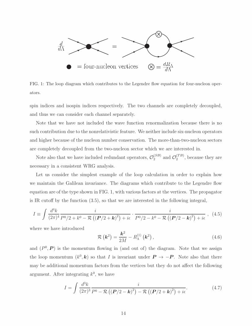
FIG. 1: The loop diagram which contributes to the Legendre flow equation for four-nucleon oper-
ators.
spin indices and isospin indices respectively. The two channels are completely decoupled,
and thus we can consider each channel separately.
Note that we have not included the wave function renormalization because there is no
such contribution due to the nonrelativistic feature. We neither include six-nucleon operators
and higher because of the nucleon number conservation. The more-than-two-nucleon sectors
are completely decoupled from the two-nucleon sector which we are interested in.
Note also that we have included redundant operators, O(SB)2 and O(TB)
2 , because they are
necessary in a consistent WRG analysis.
Let us consider the simplest example of the loop calculation in order to explain how
we maintain the Galilean invariance. The diagrams which contribute to the Legendre flow
equation are of the type shown in FIG. 1, with various factors at the vertices. The propagator
is IR cutoff by the function (3.5), so that we are interested in the following integral,
I ≡∫
d4k
(2π)4i
P 0/2 + k0 −R(
(P /2 + k)2)
+ iǫ· i
P 0/2− k0 −R(
(P /2− k)2)
+ iǫ, (4.5)
where we have introduced
R(
k2)
=k2
2M− R(1)
Λ
(
k2)
, (4.6)
and (P 0,P ) is the momentum flowing in (and out of) the diagram. Note that we assign
the loop momentum (k0,k) so that I is invariant under P → −P . Note also that there
may be additional momentum factors from the vertices but they do not affect the following
argument. After integrating k0, we have
I =
∫
d3k
(2π)3i
P 0 −R(
(P /2− k)2)
−R(
(P /2 + k)2)
+ iǫ. (4.7)
14
It is important to note that, if the IR cutoff were absent, the propagator would be
i
P 0 − P2
4M− k2
M+ iǫ
, (4.8)
where the combination P 2/4M describes the center-of-mass kinetic energy of the two nu-
cleons while k2/M represents the kinetic energy of the relative motion. It is now clear that
the only way to maintain the Galilean invariance is to cutoff the relative momentum. It is
therefore physically legitimate to replace (4.7) with∫
d3k
(2π)3i
P 0 − P2
4M− k2
M+ 2R
(1)Λ (k2) + iǫ
. (4.9)
The integral may be evaluated with an arbitrary parameter n. A useful formula for a
typical loop integral is given in Appendix A1. In the following, we consider only the sharp
cutoff limit n→ ∞, for which the RG equation becomes the simplest. We also look at the
dependence of the fixed points and the anomalous dimensions against the variation of n.
They are shown in Appendix A2.
B. RG flows and fixed points
It is useful to define the dimensionless variables as follows and write the RG equation in
terms of these variables. In the 1S0 channel, we introduce3,
x ≡ MΛ
2π2C
(S)0 , y ≡ MΛ3
2π24C
(S)2 , z ≡ Λ3
2π2B(S), (4.10)
in terms of which the RG equations are given by
dx
dt= −x−
[
x2 + 2xy + y2 + 2xz + 2yz + z2
]
, (4.11a)
dy
dt= −3y −
[
1
2x2 + 2xy +
3
2y2 + yz − 1
2z2
]
, (4.11b)
dz
dt= −3z +
[
1
2x2 + xy +
1
2y2 − xz − yz − 3
2z2
]
. (4.11c)
3 The factor M comes from the scale transformation property in nonrelativistic theory, t′ = λ2t, x′ =
λx, where λ is the scale factor. Under this transformation, the nucleon field transforms as N(t,x) =
λ3
2N ′(t′,x′), and thus we have O(S)0 = λ6O′(S)
0 for example. The d4x gives the factor λ−5, and the
additional factor λ−1 is supplied by the Λ-dependence of the coupling C(S)0 ∝ Λ−1 to cancel the λ6. To
have the right mass dimension, C(S)0 has the 1/M dependence. Similar consideration leads to the correct
Λ and M dependence of other couplings.
15
Note that the RG equations are quadratic in four-nucleon couplings due to the nonexistence
of anti-nucleons in our nonrelativistic formulation, up to the first terms, which come from
the canonical scaling.
Similarly in the 3S1–3D1 channel, we introduce
x′ ≡ MΛ
2π2C
(T )0 , y′ ≡ MΛ3
2π24C
(T )2 , z′ ≡ Λ3
2π2B(T ), w′ ≡ MΛ3
2π2
4
3C
(SD)2 , (4.12)
and we have the following RG equations,
dx′
dt= −x′ −
[
x′2+ 2x′y′ + y′
2+ 2x′z′ + 2y′z′ + z′
2+ 2w′2
]
, (4.13a)
dy′
dt= −3y′ −
[
1
2x′
2+ 2x′y′ +
3
2y′
2+ y′z′ − 1
2z′
2+ w′2
]
, (4.13b)
dz′
dt= −3z′ +
[
1
2x′
2+ x′y′ +
1
2y′
2 − x′z′ − y′z′ − 3
2z′
2+ w′2
]
, (4.13c)
dw′
dt= −3w′ −
[
x′w′ + y′w′ + z′w′
]
. (4.13d)
Note that the RG equations (4.13) for the 3S1–3D1 channel are identical to the RG equations
(4.11) for the 1S0 channel if w′ is set equal to zero. (This is actually a solution.)
We can now draw the RG flow diagram. FIG. 2 shows the RG flow for the 1S0 channel
and FIG. 3 for the 3S1–3D1 channel up to operators with dimension eight. Both flows are
projected on to the two-dimensional plane spanned by the lowest order coupling constants.
As expected from the RG equations (4.11) and (4.13), the RG flows for the 1S0 channel and
for the 3S1–3D1 channel have similar structure. First of all, there are two fixed points in
both RG flows; the trivial IR fixed point and the non-trivial UV fixed point. Secondly, both
RG flows have two phases ; one in which all points approaches the trivial fixed point in the
limit of vanishing cutoff, and the other one in which all points approaches infinity at certain
finite cutoff scale. The nontrivial fixed points are on the phase boundaries.
Location of the fixed points are given by solutions of the equations, dx/dt = dy/dt =
dz/dt = 0, for the 1S0 channel, and dx′/dt = dy′/dt = dz′/dt = dw′/dt = 0 for the 3S1–3D1
channel. As explained in Appendix A2, we find four fixed points in each channel for an
arbitrary value of the parameter n. One of them is extremely unstable against the variation
of n, and may be considered as “spurious”, i.e., it is an artifact of our truncation. The rest
are stable and take the following values in the n→∞ limit,
16
-1
-0.5
0
0.5
1
-1.5 -1 -0.5 0 0.5 1
y
x
FIG. 2: The RG flow for the 1S0 channel
projected onto the C(S)0 –C
(S)2 plane. Flow
lines start with the arbitrarily chosen value
z = 0 at the edges of the graph.
-1
-0.5
0
0.5
1
-1.5 -1 -0.5 0 0.5 1
y’
x’
FIG. 3: The RG flow for the 3S1–3D1
channel projected onto the C(T )0 –C
(T )2 plane.
Flow lines start with the arbitrarily chosen
values z′ = 0 and w′ = 0.1 at the edges of
the graph.
1S0 channel:
(x⋆, y⋆, z⋆) = (0, 0, 0) ,
(
−1,−12,1
2
)
,
(
−9, 152,−3
2
)
(4.14)
3S1–3D1 channel:
(
x′⋆, y′
⋆, z′
⋆, w′⋆) = (0, 0, 0, 0) ,
(
−1,−12,1
2, 0
)
,
(
−9, 152,−3
2, 0
)
. (4.15)
We also disregard the third fixed points in both channels, because they are irrelevant to
the discussion of the power counting. The eigenoperators at these fixed points are complex
and have complex eigenvalues (scaling dimensions). It means that the operators do not have
the definite scaling property there.
We obtain the scattering amplitudes explicitly in both channels in Appendix B as we
did in the previous paper[27], and find that the RG equations, which look much more
complicated than (4.11) and (4.13), have only two fixed points in each channel and they
exactly agree with the first two fixed points obtained here4.
4 Actually, the RG equation obtained in the previous paper[27] is those for the 1S0 channel.
17
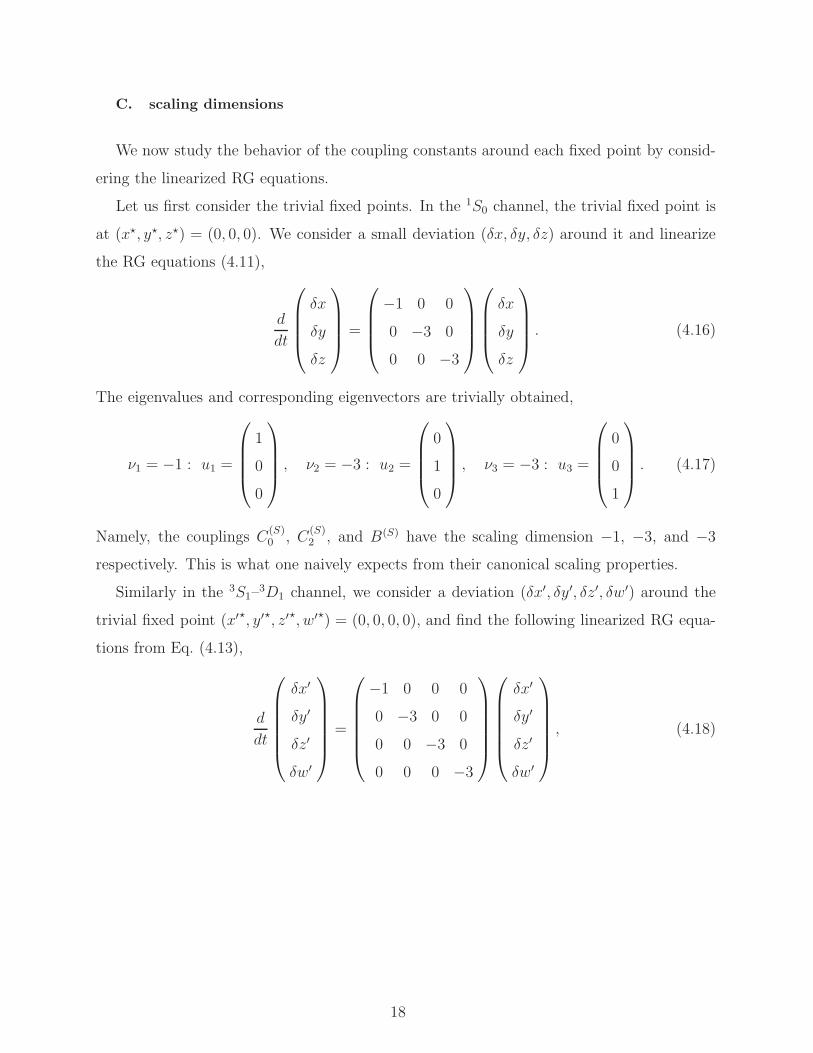
C. scaling dimensions
We now study the behavior of the coupling constants around each fixed point by consid-
ering the linearized RG equations.
Let us first consider the trivial fixed points. In the 1S0 channel, the trivial fixed point is
at (x⋆, y⋆, z⋆) = (0, 0, 0). We consider a small deviation (δx, δy, δz) around it and linearize
the RG equations (4.11),
d
dt
δx
δy
δz
=
−1 0 0
0 −3 0
0 0 −3
δx
δy
δz
. (4.16)
The eigenvalues and corresponding eigenvectors are trivially obtained,
ν1 = −1 : u1 =
1
0
0
, ν2 = −3 : u2 =
0
1
0
, ν3 = −3 : u3 =
0
0
1
. (4.17)
Namely, the couplings C(S)0 , C
(S)2 , and B(S) have the scaling dimension −1, −3, and −3
respectively. This is what one naively expects from their canonical scaling properties.
Similarly in the 3S1–3D1 channel, we consider a deviation (δx′, δy′, δz′, δw′) around the
trivial fixed point (x′⋆, y′⋆, z′⋆, w′⋆) = (0, 0, 0, 0), and find the following linearized RG equa-
tions from Eq. (4.13),
d
dt
δx′
δy′
δz′
δw′
=
−1 0 0 0
0 −3 0 0
0 0 −3 0
0 0 0 −3
δx′
δy′
δz′
δw′
, (4.18)
18
with the eigenvalues and corresponding eigenvectors,
ν1 = −1 : u1 =
1
0
0
0
, ν2 = −3 : u2 =
0
1
0
0
, ν3 = −3 : u3 =
0
0
1
0
,
ν4 = −3 : u4 =
0
0
0
1
. (4.19)
The coupling constants C(T )0 , C
(T )2 , B(T ), and C
(SD)2 have the scaling dimension −1, −3, −3,
and −3 respectively.
Note that all of the scaling dimensions are negative at the trivial fixed point and thus
the corresponding operators are irrelevant, i.e., they should be treated perturbatively.
At the nontrivial fixed point, on the other hand, something much more interesting hap-
pens. In the 1S0 channel, the deviations from the nontrivial fixed point (x⋆, y⋆, z⋆) =
(−1,−1/2, 1/2) satisfy the following linearized RG equations,
d
dt
δx
δy
δz
=
1 2 2
2 0 1
−2 −2 −3
δx
δy
δz
, (4.20)
with the eigenvalues and corresponding eigenvectors,
ν1 = +1 : u1 =
1
1
−1
, ν2 = −1 : u2 =
0
−11
, ν3 = −2 : u3 =
2
−1−2
. (4.21)
Note that the scaling dimensions change drastically. Note also that the eigenoperators are
not monomials but linear combinations of the operators. This is a typical feature of the
momentum cutoff regularization.
Similar results are obtained in the 3S1–3D1 channel, where the linearized equations around
19
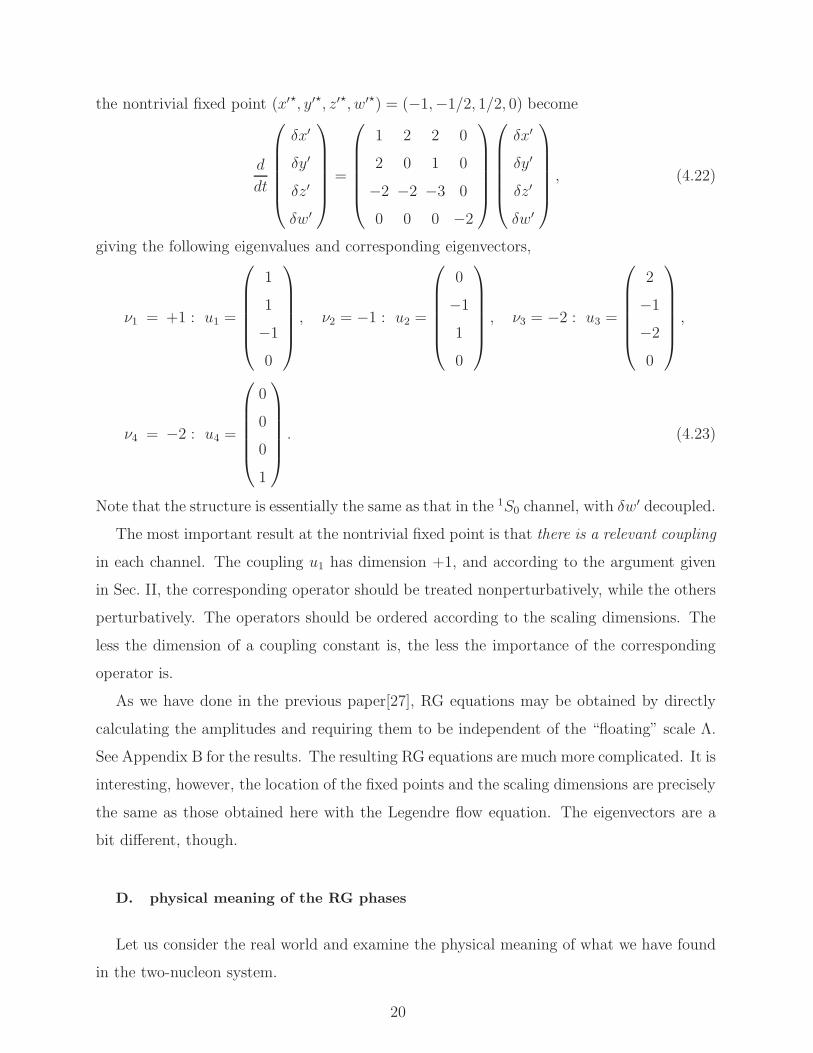
the nontrivial fixed point (x′⋆, y′⋆, z′⋆, w′⋆) = (−1,−1/2, 1/2, 0) become
d
dt
δx′
δy′
δz′
δw′
=
1 2 2 0
2 0 1 0
−2 −2 −3 0
0 0 0 −2
δx′
δy′
δz′
δw′
, (4.22)
giving the following eigenvalues and corresponding eigenvectors,
ν1 = +1 : u1 =
1
1
−10
, ν2 = −1 : u2 =
0
−11
0
, ν3 = −2 : u3 =
2
−1−20
,
ν4 = −2 : u4 =
0
0
0
1
. (4.23)
Note that the structure is essentially the same as that in the 1S0 channel, with δw′ decoupled.
The most important result at the nontrivial fixed point is that there is a relevant coupling
in each channel. The coupling u1 has dimension +1, and according to the argument given
in Sec. II, the corresponding operator should be treated nonperturbatively, while the others
perturbatively. The operators should be ordered according to the scaling dimensions. The
less the dimension of a coupling constant is, the less the importance of the corresponding
operator is.
As we have done in the previous paper[27], RG equations may be obtained by directly
calculating the amplitudes and requiring them to be independent of the “floating” scale Λ.
See Appendix B for the results. The resulting RG equations are much more complicated. It is
interesting, however, the location of the fixed points and the scaling dimensions are precisely
the same as those obtained here with the Legendre flow equation. The eigenvectors are a
bit different, though.
D. physical meaning of the RG phases
Let us consider the real world and examine the physical meaning of what we have found
in the two-nucleon system.
20
As mentioned in Introduction, the two-nucleon system is considered as “fine-tuned,” in
the sense that the scattering length is unnaturally large. It suggests that the actual system
is near the nontrivial fixed point in each channel. The closer to the fixed point it is, the
longer the scattering length is.
What then makes the physical difference between the 1S0 and the 3S1–3D1 channels, both
of which are close to the nontrivial fixed points? The answer to this question is provided
by the flow diagram; the nontrivial fixed point is on the boundary between two phases. In
one of them, the flow goes toward the trivial fixed point in the IR. We therefore call this the
weak coupling phase. In the other, the flow goes toward stronger couplings, thus we call it
the strong coupling phase. It is natural to think that the real two-nucleon system in the 1S0
channel, in which there is no bound state, is in the weak coupling phase, while that in the
3S1–3D1 channel, in which there is a shallow bound state, deuteron, is in the strong coupling
phase.
In order to make the physical picture more transparent, it is useful to examine the four-
nucleon (two-nucleon scattering) amplitudes. As shown in Ref. [27] and in Appendix B,
the four-nucleon amplitudes may be obtained explicitly in the derivative expansion. By
substituting the solution of the linearized RG equation in the 1S0 channel obtained from the
direct method,
δx
δy
δz
= a
2
1
−4
(
Λ
Λ0
)2
+ b
0
−11
(
Λ
Λ0
)
+ c
1
1
−1
(
Λ0
Λ
)
, (4.24)
where a, b, and c are small dimensionless constants, into the amplitude in the center-of-mass
frame, we obtained the renormalized (off-shell) amplitude near the nontrivial fixed point[27],
A−1(p0,p′2,p2)∣
∣
∣
∗= −M
4π
[
2c
πΛ0 −
4b
π
(
Mp0
Λ0
)
− i√
Mp0]
+ · · · . (4.25)
where ellipsis denotes higher orders in 1/Λ0.
By comparing it with the effective range expansion,
A−1∣
∣
on−shell= −M
4π
[
− 1
α+
1
2rp2 − ip
]
+ · · · , (4.26)
on the mass shell p =√
Mp0 = |p| = |p′|, one sees the scattering length α and the effective
21
range r are given by
α = − π
2cΛ0
, r = − 8b
πΛ0
. (4.27)
That is, the inverse of the scattering length is identified as the relevant coupling. The fine-
tuning |α| ≫ Λ−10 indeed corresponds to |c| ≪ 1. It is also important that the sign of the
coupling c distinguishes the phases, namely, the inverse of the scattering length is the order
parameter. It vanishes on the boundary, the critical surface. Because the effective range is
of natural size, r ∼ Λ−10 , it is more accurate to say that the real two-nucleon system is close
to the critical surface.
The location of the pole which is found within the range of EFT is given by
p0 ≃ −Λ2
0
M
(
2c
π
)2 [
1 +16bc
π2
]
. (4.28)
A similar expression is obtained for the pole in the 3S1–3D1 channel. The pole on the
physical Riemann sheet that corresponds to a bound state occurs only when c < 0, i.e., in
the strong coupling phase, while there is no restriction on b.
V. COMMENTS ON OTHER POWER COUNTING SCHEMES
As we emphasized in Sec. II, our way of determining the power counting on the basis of
the scaling dimensions is general and nonperturbative. It does not depend on any specific
regularization/renormalization scheme, nor on which fixed point we are looking at.
In this section, we would like to comment on other works from our point of view and make
the connection between their power counting and ours. It leads us to a deeper understanding
of the power counting issues.
First of all, we would like to mention the work done by Birse, McGovern, and
Richardson[26], which is very close to ours in philosophy. They consider the most gen-
eral potential and the Wilsonian RG equation satisfied by it. The “fixed point” potential
depends only on the energy,
V0(p,Λ) = −2π2
M
[
Λ− p
2ln
Λ + p
Λ− p
]−1
, (5.1)
where p =√ME, with the E being the center-of-mass energy. They then consider the
perturbation around the “fixed point” potential, and find the eigenvalues of the linearized
RG equations. The first few eigenvalues coincide with ours. They use the information to
22
determine the power counting. It is important to note that the “energy-dependent perturba-
tions” have the spectrum ν = −1, 1, 3, · · · , while the “momentum-dependent perturbations”
have ν = 2, 4, 5, · · · . (Note that their ν’s have opposite signs to the scaling dimensions used
in this paper.)
To compare their results with ours, it is useful to translate our operator formulation to
the potential one. Our operators may be equivalent to the potential,
V (p0,p,p′) = C0 + 4C2(p2 + p′2)− 2B
(
p0 − p2 + p′2
2M
)
+ · · · , (5.2)
where we suppress the superscripts which denote the channel. If we substitute the fixed
point values of the couplings, we have
V ⋆(p0,p,p′) = − 2π2
MΛ
[
1 +Mp0
Λ2
]
+ · · · , (5.3)
which is exactly the expansion of the potential (5.1), with p0 replaced by E. Note that the
momentum dependence cancels at the fixed point. This may be an evidence that both ap-
proaches are essentially the same. Actually, the “perturbations” with the scaling dimensions
ν1 = 1 and ν2 = −1 corresponds to the potentials that depends only on p0, while that with
ν3 = −2 to a momentum-dependent one, in agreement with their findings5.
For this simplest pionless NEFT in the two-nucleon sector, the method based on the
potential has an advantage. On the other hand, because our approach is based on the general
principle of fully-fledged quantum field theory, we could treat more complicated systems in
a unified and systematic way. For example, we could treat three-nucleon problems without
worrying about the off-shell ambiguities, and fully relativistic systems for which the potential
picture is not valid. The important point is that our work gives a field-theoretical foundation
for their approach and has opened a window to wider applications.
In the following, we will make comments on other power counting schemes on the basis
of what we have found.
In Weinberg’s scheme[5, 6], one assumes the NDA power counting in making the “effective
potential,” then treats it nonperturbatively. As we have explained, however, the NDA is the
power counting near the trivial fixed point, where all the operators are irrelevant and should
5 A careful study reveals that the eigenvector for ν3 = −2 does not agree with theirs, though those for
ν1 = 1 and ν2 = −1 do. The reason seems that the reaction matrix they consider does not have a direct
connection to the scattering amplitude which we work with off the mass shell.
23
be treated perturbatively. The so-called infrared enhancement due to two-nucleon reducible
diagrams somehow remedies the above-mentioned mismatch in the treatment; it makes the
“effective potential” more relevant. The way is not systematic however, and in some cases
inconsistent[16].
The scheme due to Kaplan, Savage, and Wise[18, 19] is important because they em-
phasized one of the most important aspects of the two-nucleon system; it is close to the
nontrivial fixed point! (The existence of the nontrivial fixed point itself had been noticed
by Weinberg[6].) It is however very subtle why the KSW scheme succeeds in some channels,
and fails in others. To understand the points, we have to examine it very carefully.
It is difficult to define the KSW power counting without mentioning the Power Divergence
Subtraction (PDS) scheme6. In PDS, the poles at D = 3 as well as D = 4 are subtracted.
In the pionless NEFT, there is no pole at D = 4, so that one subtracts as if one were
in D = 3 dimensions. This is the heart of the PDS scheme; it changes the (canonical)
dimensions of the operators! For example, the operator O(S)0 has the canonical dimension
6 in D = 4 dimensions, but would have 4 in D = 3 dimensions. In PDS, it is treated as
an operator of dimension 4. This shift of the dimension by two coincides with the correct
anomalous dimension of the operator, as we found in the previous section. (Remember that
the leading contact operators have anomalous dimension 2, and according to Birse et al., all
the “energy-dependent perturbations” seem to have the same anomalous dimensions.) We
believe that it is the true reason why the KSW/PDS scheme works near the nontrivial fixed
point7.
Actually, this “shift by two” applies to all the four-nucleon operators in the KSW/PDS
scheme8. To see this, consider the KSW/PDS RG equation for the dimensionless couplings,
µdγ2ndµ
= (2n+ 1)γ2n +n∑
m=0
γ2mγ2(n−m), (5.4)
where γ2n ≡ (Mµ2n+1/4π)C2n, with C2n(µ) being given in Eq. (2.10) in Ref. [19]. Near the
6 We do not claim that PDS is indispensable for the KSW power counting, but that the PDS scheme
provides the most unambiguous definition of the KSW power counting.7 From this point of view, it is legitimate to think that the KSW/PDS scheme should be applied only to
the case near the nontrivial fixed point, though the RG equations (5.4) know about the trivial fixed point
too.8 The redundant operators scales differently than the others, but they are not necessary with dimensional
regularization.
24
nontrivial fixed point (γ⋆0 , γ⋆2 , γ
⋆4 , · · · ) = (−1, 0, 0, · · · ), the RHS of (5.4) becomes
(2n+ 1)γ2n + 2γ0γ2n + · · · ≃ (2n− 1)γ2n, (5.5)
where the ellipsis stands for terms quadratic in γ’s and independent of γ0, which do not
contribute to the anomalous dimensions. This explicitly shows the shift from (2n + 1) to
(2n− 1)9.
As far as all the anomalous dimensions are two, the KSW/PDS scheme would work
perfectly. The problem in the pionful NEFT seems that the singular interactions due to pion
exchange in the 3S1–3D1 channel would modify the anomalous dimensions of the contact
operators strongly, making the “shift by two” rule invalid. Actually, Birse[22] found that the
anomalous dimensions shift additionally by minus one half at the nontrivial fixed point in
the presence of the tensor force due to one-pion exchange. The investigation in this direction
is currently in progress[31].
Several authors considered power countings which are compatible with the KSW power
counting without using PDS so that one might think that the KSW scheme may be defined
independent of PDS. In fact, it appears possible to do so if one assumes the scaling of the
coupling constants which is a consequence of the PDS regularization/renormalization. In
Ref. [32], van Kolck introduced a scale ℵ, which accounts for the fine-tuning, and assumed
the scaling of the coupling constants without specifying the regularization/renormalization.
The scale ℵ seems to correspond to our cΛ0 with c ≪ 1 introduced in Eq. (4.24). It is
important to note that ℵ is a physical scale so that there is no notion of RG with respect to
ℵ in his approach. If one nevertheless identifies ℵ with the scale µ in the KSW scheme, the
assumed scaling of the couplings is just the one in the KSW/PDS scheme. On the other hand,
using momentum space subtraction renormalization, Mehen and Stewart[33, 34] imposed the
renormalization condition (Eq. (6) in Ref. [33])
iA(m−1)∣
∣
p=iµR,mπ=0= −iC2m(µR) (iµR)
2m , (5.6)
9 There is a subtle point about the scaling of the coupling constants. If one solves the RG equations near the
fixed point, the coupling constant scales C2n ∼ 4π/MΛ2n−10 µ2, but it is different from the KSW scaling
C2n ∼ 4π/MΛn0µ
n+1. It is due to the assumption that the effective range is of natural size, r ∼ 1/Λ0.
Namely, the KSW scaling is not that for a point close to the fixed point, but for a point close to the
critical surface.
25
on the (part of the) amplitude that scales as Qm−1, where Q is a typical momentum
scale. (This power counting for the amplitudes is also assumed in accordance with the
KSW/PDS scheme.) Putting µR ∼ Q, it requires the coupling constant C2m(µR) to scale as
∼ Qm−1 (µR)−2m ∼ Q−(m+1), which is essentially equivalent to the KSW/PDS power count-
ing. It is still unclear to us why the renormalization condition (5.6) reflects the situation
that we are close to the nontrivial fixed point.
Let us finally comment on the confusion in the literature over the scale µ introduced in
dimensional regularization. It is important to note that the scale µ does not have intrinsic
meaning of “typical scale.” It is completely arbitrary and physics is independent of it. In
the usual applications of dimensional regularization to relativistic field theory, µ appears in
logarithms as ln (Q2/µ2), where Q is the typical scale of the process. It is this dependence
that makes it useful to think µ ∼ Q in order to suppress the “large logarithms.” In our
application to NEFT, however, there is no logarithm, thus no reason to think µ ∼ Q.
VI. CONCLUSION
In this paper we studied the Wilsonian RG flow of pionless NEFT using the Legendre
flow equation in order to determine the correct power counting. We emphasized that the
determination of power counting should be based on the scaling dimensions, because power
counting is in essence the order of magnitude estimate based on dimensional analysis, and
the scaling dimensions are quantum dimensions of the operators.
The RG flow has a nontrivial fixed point as well as a trivial one in each of the 1S0 and
3S1–3D1 channels. Near the nontrivial fixed point, we found a relevant operator, the coupling
constant of which is proportional to the inverse of the scattering length. The nontrivial fixed
point is on the boundary of two phases, the weak coupling and the strong coupling phases.
The inverse of the scattering length is regarded as the order parameter, which takes zero
at the boundary. The real two-nucleon systems are considered to be close to the nontrivial
fixed point.
The difference between the 1S0 and 3S1–3D1 channels comes from the difference of the
phases they are in. In the strong coupling phase, the scattering length is positive and the
four-nucleon amplitude has a physical pole which represent a bound state, the deuteron in
the 3S1–3D1 channel, while in the weak coupling phase, the scattering length is negative and
26
there is no bound state; this phase describes the 1S0 channel. We believe that this way of
viewing the difference between the two channels is new, and we expect that it would give
some further insight into the character of nuclear force.
The relation to the work by Birse et al. was clarified. The use of fully developed EFT
framework was emphasized. We also made comments on other power counting schemes and
tried to understand why they succeed in some cases and fail in others from our point of
view. In particular, we claimed that the true reason why the KSW/PDS scheme works is
identified as the “shift by two,” namely, PDS happens to capture the essential feature that
the anomalous dimensions of the contact two-nucleon interactions are two.
It was essential to include the so-called redundant operators to consistently perform the
Wilsonian RG analysis[27] in a fully field theoretical manner. They are also necessary to
renormalize the off-shell amplitudes. The inclusion of them seems essential to consider the
tree-nucleon systems.
The RG equations derived from the Legendre flow equation are much simpler than those
from the amplitude, while the important physical information (the existence and the location
of fixed points, the global structure of the flows, the scaling dimensions, etc.) is the same.
The use of the Legendre flow equation would help us to tackle more difficult problems, where
the direct method seems infeasible.
It is very important to apply the present method based on the Wilsonian RG to determine
the power counting of the pionful NEFT, where the power counting issues are most contro-
versial. The singular tensor force would change the anomalous dimension of the lowest-order
contact operator drastically in the 3S1–3D1 channel, invalidating the “shift by two” rule. One
might imagine that, at a high energy scale, there is actually no difference of the values of
couplings between the 1S0 and 3S1–3D1 channels, but the pion interactions make them so
different. This scenario appears attractive from the approximate spin-flavor symmetry point
of view[35, 36, 37]. Note that the nontrivial fixed point is spin-flavor symmetric.
One of the interesting results in this paper is the explicit relation between the Wilsonian
RG analysis and the existence of the bound state in the strong coupling phase. It would
open a new possibility of studying bound states using the Wilsonian RG. On the other hand,
it would become important when we study the tree-nucleon systems without introducing a
“dibaryon” field [38, 39, 40]. Note that most of the existing literature on the NEFT study
of three-nucleon systems is based on the “dibaryon” formalism. Because our formulation is
27
fully field theoretical, it is free from the off-shell ambiguities which the approaches based on
potentials suffer from.
Acknowledgments
We would like to thank Y. Yamamoto for several useful discussions. We are also grateful
to H. Gies for pointing out the wrong placing of the derivative ∂t in Sec. III in the earlier
manuscript. One of the authors (K.H.) is partially supported by Grant-in-Aid for Scientific
Research on Priority Area, Number of Area 763, “Dynamics of Strings and Fields,” from
the Ministry of Education, Culture, Sports, Science and Technology, Japan.
APPENDIX A: IR CUTOFF FUNCTION WITH FINITE n
In this Appendix, we give a useful formula involving the IR cutoff function, and the
dependence of the fixed points and the scaling dimensions of the RG equations on n.
1. Evaluation of a typical loop integral
A typical loop integral with the IR cutoff function R(1)Λ (k2) which appears repeatedly in
the derivation of our RG equations is
Im,n ≡∫
d3k
(2π)3∂t
(k2)m
A(P )− k2
M+ 2R
(1)Λ (k2)
, (A1)
where A(P ) is a Galilean invariant quantity,
A(P ) ≡ P 0 − P 2
4M, (A2)
and P µ = (P 0,P ) is the momentum flowing in (and out of) the diagram, P = p1 + p2 =
p3+p4, where p1 and p2 are initial momenta, and p3 and p4 are final momenta of the nucleons.
The IR cutoff function is chosen as (3.5) for definiteness.
Switching to the polar coordinate, making the change of variable to x = k/Λ, and ex-
28
panding the integrand with respect to A(P ) ≡ (M/Λ2)A(P ), we have
Im,n = − n
π2MΛ2m+1
∫ ∞
0
dxx2n+2m+4 exp(
x2n)
R(x)
A(P )− x2(
1− R(x))
2
= −MΛ2m+1
2π2
[
Γ
(
1 +2m+ 1
2n
)
+ A(P )Γ
(
1 +2m− 1
2n
)
(
2− 21−2m2n
)
+O(A2)
]
,
(A3)
where R(x) ≡ (1− exp (x2n))−1
has been introduced. In the present paper, we disregard the
terms of O(A2) as higher orders.
We may decompose A(P ) into the following Galilean invariant quantities,
A(P ) =
(
p01 −p21
2M
)
+
(
p02 −p22
2M
)
+1
4M(p1 − p2)
2 . (A4)
Combining possible multiplicative momentum factors outside the integral, we can identify
the contributions to the various operators in our theory space. For example, contributions
from the first two terms renormalize a redundant operator and the last term does the oper-
ators which contain spatial derivatives.
2. Dependence on the IR cutoff function
The RG equations are derived and solved with a finite value of n. In this section, we
show the n dependence of the fixed points and the scaling dimensions.
The dependence on n might give some useful information on the behavior of the present
approximation. Note that if no approximation were made, the universal quantities such as
the scaling dimension would not depend on how the RG transformation is defined. Weak
dependence would suggest that the approximation is good. We will see shortly that the
most of the fixed points as well as the scaling dimensions have very weak dependence. The
fixed point with strong dependence on n may be regarded as “spurious” and, for other fixed
points, the approximation is very good.
In general, a sharp momentum cutoff gives a poor convergence and a smooth cutoff
function is preferred[41]. In the present case, however, the dependence on n is very weak
and the use of a sharp cutoff is expected to be reasonable. In addition, it gives the simplest
expressions.
29
TABLE I: The dependence on n of the fixed point A.
n location of the fixed point(x⋆, y⋆, z⋆) scaling dimensions
2 (−1.10326,−0.60467, 0.60467) (−2,−1, 1)
10 (−1.02722,−0.524991, 0.524991) (−2,−1, 1)
102 (−1.00287,−0.502587, 0.502587) (−2,−1, 1)
103 (−1.00029,−0.50026, 0.50026) (−2,−1, 1)
104 (−1.00003,−0.599926, 0.500026) (−2,−1, 1)
∞ (−1,−12 ,
12) (−2,−1, 1)
For a finite value of n, we find four fixed points including the trivial one. The dependence
of the three nontrivial fixed points in the 1S0 channel is given in Tables I, II, and III. (The
dependence is similar for the 3S1–3D1 channel.) The last column shows the three eigenvalues
of the linearized RG equations at the fixed point. Let us call these fixed points A, B, and
C.
Note that, although we have an analytic expression for the RG equations for any n,
the actual evaluation is done with the aid of a computer. We use Mathematica, but some
numerical errors are not avoidable.
One can easily see that the fixed points A and B have little n dependence (for n ≥ 10),
while the fixed point C depends on n strongly. We disregard the fixed point C. Note that
even for the smallest integer value of n, n = 2 (n = 1 does not satisfy the condition (3.4).),
the scaling dimensions for the fixed point A are the same while the fixed points B and C
disappear there.
The fixed point B has complex eigenvalues, though they have weak dependence on n. As
discussed in the main text, the eigen-operators do not have the definite scaling properties
there and we disregard it too in our discussion of the power counting. At the moment we
know neither if it is just an artifact, nor, even if it is not, its physical implications.
30
TABLE II: The dependence on n of the fixed point B.
n location of the fixed point(x⋆, y⋆, z⋆) scaling dimensions