Kolmogorov-Chaitin Complexity of Linear Digital ...

Kolmogorov-Chaitin Complexity of Linear DigitalControllers Implemented using Fixed-point Arithmetic

James F. Whidborne∗, John Mckernan∗, Da-Wei Gu†

[email protected]

†Department of Engineering, University of Leicester

∗Department of Aerospace Sciences, Cranfield University

Kolmogorov-Chaitin Complexity of Linear Digital Controllers Implemented using Fixed-point Arithmetic – p. 1/24

Introduction

• Modern control design methods may give high-order digital controllers— regarded as complex, thus costly & difficult to implement

• Rounding errors occur in digital controller implementations — magnifiedwith controller order — often solved using costlier longer word-length orfloating point processors

• Hence control system designers motivated to produce low-ordercontrollers


Introduction

• Modern control design methods may give high-order digital controllers— regarded as complex, thus costly & difficult to implement

• Rounding errors occur in digital controller implementations — magnifiedwith controller order — often solved using costlier longer word-length orfloating point processors

• Hence control system designers motivated to produce low-ordercontrollers

But do low-order controllers have lower complexity?


Introduction

For example consider : K1(z) =1

(z + 1)3and K2(z) =

1

z + 0.1

• controller K1 has order 3 & controller K2 has order 1

• normal assumption: K2 has lower complexity than K1


Introduction


(z + 1)3and K2(z) =

1

z + 0.1



BUT• K1 requires 0 multiplication operations & can be implemented exactly• K2 requires 1 multiplication operation & cannot be implemented exactly!

(0.1 in base-2 is 0.000110011 · · · recurring — hence cannot berepresented exactly by binary computer with finite wordlength)

• hence K2 has a higher complexity than K1


Introduction


(z + 1)3and K2(z) =

1

z + 0.1



BUT• K1 requires 0 multiplication operations & can be implemented exactly• K2 requires 1 multiplication operation & cannot be implemented exactly!

(0.1 in base-2 is 0.000110011 · · · recurring — hence cannot berepresented exactly by binary computer with finite wordlength)

• hence K2 has a higher complexity than K1

Controller order is only an indicator of controller complexity!

Required word-length and the arithmetic operations are other factors thatdetermine controller complexity


Introduction

• To measure complexity accurately, we use the idea ofKolmogorov-Chaitin complexity: the complexity of a computable object ismeasured by the length, in bits, of the shortest program that computesthe object

• We consider the complexity of linear, fixed-point arithmetic, digitalcontrollers from a Kolmogorov-Chaitin perspective

• The complexity of designs for the restricted complexity controllerbenchmark problem are investigated

• It will be seen that, from a Kolmogorov-Chaitin viewpoint, higher-ordercontrollers with a shorter word-length may have a lower complexity but abetter performance than lower-order controllers with longer word-length


Kolmogorov-Chaitin complexity

• Measures the complexity of a computable object by the length, in bits, ofthe shortest program that computes the object.

Definition 1. The Kolmogorov complexity ΓU (x) of a computable finite-length binarystring, x, with respect to a universal Turing machine U is defined as

ΓU (x) = minp:U(p)=x

ℓ(p)

where p denotes a program interpreted by U and ℓ(p) denotes the description length ofp.



• Measures the complexity of a computable object by the length, in bits, ofthe shortest program that computes the object.

Definition 1. The Kolmogorov complexity ΓU (x) of a computable finite-length binarystring, x, with respect to a universal Turing machine U is defined as

ΓU (x) = minp:U(p)=x

ℓ(p)

where p denotes a program interpreted by U and ℓ(p) denotes the description length ofp.

• Digital controllers are not implemented on universal Turing machines —the following well-known theorem relates Kolmogorov complexity to thelength complexity using some other computing machine

Theorem 1. If U is a universal computer, then for any other computer A,

ΓU (x) ≤ ΓA(x) + cA

for all binary strings x where the constant cA does not depend on x.



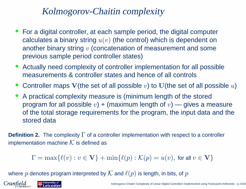
• For a digital controller, at each sample period, the digital computercalculates a binary string u(v) (the control) which is dependent onanother binary string v (concatenation of measurement and someprevious sample period controller states)

• Actually need complexity of controller implementation for all possiblemeasurements & controller states and hence of all controls

• Controller maps V(the set of all possible v) to U(the set of all possible u)• A practical complexity measure is (minimum length of the stored

program for all possible v) + (maximum length of v) — gives a measureof the total storage requirements for the program, the input data and thestored data

Definition 2. The complexity Γ of a controller implementation with respect to a controllerimplementation machine K is defined as

Γ = max{ℓ(v) : v ∈ V} + min{ℓ(p) : K(p) = u(v), for all v ∈ V}

where p denotes program interpreted by K and ℓ(p) is length, in bits, of p


Complexity of state-space realizations

State space representation Ks = (A, B, C, D), with n states, p inputs and qoutputs, where at the ith time step

x(i + 1) = Ax(i) + By(i), u(i) = Cx(i) + Dy(i)

Let k be the concatenated binary string of the parameters of Ks

• If the chosen word-length is w, then the length of k is given byℓ(k) = (n + p)(n + q)w and the length of v is given by ℓ(v) = (n + p)wand thus the required data storage of Ks is ℓ(k) + ℓ(v)

• This is not a satisfactory complexity measure, because it does notconsider the possibility of sparse realizations, where some of thecontroller parameters are zero or unity

• No multiplication or addition operation if a controller parameter is zero• No multiplication operation if a controller parameter is unity

Hence need to measure complexity using Definition 2 (i.e. measure programlength, not data storage)


Evaluating complexity of LTI controllers

Definition 2 complexity of a linear time-invariant controller easily evaluated:• v has constant length• program is independent of u, y and x

• hence program length ℓ(p) is independent of v and u

Length of the program ℓ(p) also depends on implementation machine K i.e. isthere hardware support for floating point calculations, multiplicationoperations etc? If so, what length “overhead” is given for the use of morecomplex operations over simpler operations such as addition or barrel shift?

• Simple computing devices preferred for reasons of cost and reliability• In this paper, assume device has fixed point arithmetic and multiplication

is by sequence of additions and barrel shifts (i.e. one addition + one shiftper unity bit of the constant multiplicand)


Complexity of state-space realizations

Thus the following complexity measure is proposed:Definition 3. The controller complexity Γ(Ks) of a state space controller realization

Ks = (A, B, C, D) is given by

Γ(Ks) = ℓ(v) +

ℓ(k)∑

i=1

ki

where the concatenated binary string of the parameters of Ks is given byk = [k1, k2, . . . , kℓ(k)], ki ∈ {0, 1}.

This gives a measure of the length of program in terms of number ofoperations and data storage requirements


Other controller realizations

State space realization is over-parameterized, in that there are a largenumber of degrees of freedom in the choice of the (A, B, C, D) termsOther common realizations are:

• Parallel and the cascade forms — considered here• The direct form (obtained directly from the difference equation) is

numerically unreliable for medium and high-order controllers — hencenot considered here

• Open-loop stability of the lattice form can be determined by inspection— advantageous in pre-MATLAB era — hence not considered here


Complexity of parallel and cascade realizations

Parallel and cascade realizations decompose controller into first andsecond-order direct-form filter blocks:

F (z) =a0 + a1z

−1

1 + b1z−1and F (z) =

a0 + a1z−1 + a2z

−2

1 + b1z−1 + b2z−2

• The parallel structure used here is (for SISO controllers)

Kp(z) =

m∑

i=1

Fi(z)

where each Fi is a first or second order transfer function• The cascade structure is given by

Kc(z) =

m∏

i=1

Fi(z)


Complexity of cascade realization

• Assume m filter blocks — all second order• c is the concatenated binary string representation of all filter block

parameters a0, a1, a2, b1, b2

• Length of c is thus ℓ(c) = 5mw where w is the word-length

• Each filter block requires two previous outputs and two previous inputsto be stored, but two previous outputs of each block (except the last) areequal to the two previous inputs of the next block

• Hence length of v is given by ℓ(v) = (2m + 3)w (measurement must alsobe stored)

Definition 4. The controller complexity Γ(Kc) of a cascade controller realization Kc is givenby

Γ(Kc) = ℓ(v) +

ℓ(c)∑

i=1

ci

where c = [c1, c2, . . . , cℓ(c)], ci ∈ {0, 1}.


Restricted complexity controller benchmark

• Plant is a hydro-suspension system subjected to a disturbance• Objective is to design the simplest controller that meets some control

specifications

K G- - - -?u y

Gp

+

+

?up

p

• The objective of the control is to reduce the residual force, y, at the firstand second vibration modes of the primary plant, Gp

• The residual force y is measured and fed back to the secondary plant viaa digital controller, K

• Controller gain should be zero at Fs/2, which is achieved by ensuringthe controller includes the term (z−1 + 1)



Control specifications are

• output sensitivity function Syp = (1 + KG)−1 constrained in frequencydomain by function Fyp(ω)

• input sensitivity function Sup = −K(1 + KG)−1 constrained in frequencydomain by function Fup(ω)



Control specifications are

• output sensitivity function Syp = (1 + KG)−1 constrained in frequencydomain by function Fyp(ω)

• input sensitivity function Sup = −K(1 + KG)−1 constrained in frequencydomain by function Fup(ω)

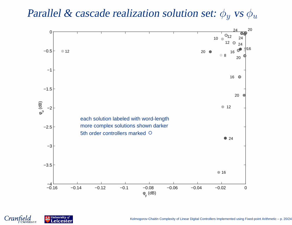
Two performance measures are thus defined as

φy = maxω∈[0,ωs/2]

(Syp(ω) − Fyp(ω))

φu = maxω∈[0,ωs/2]

(Sup(ω) − Fup(ω))

where ωs = is sampling frequency


State-space realization controllers

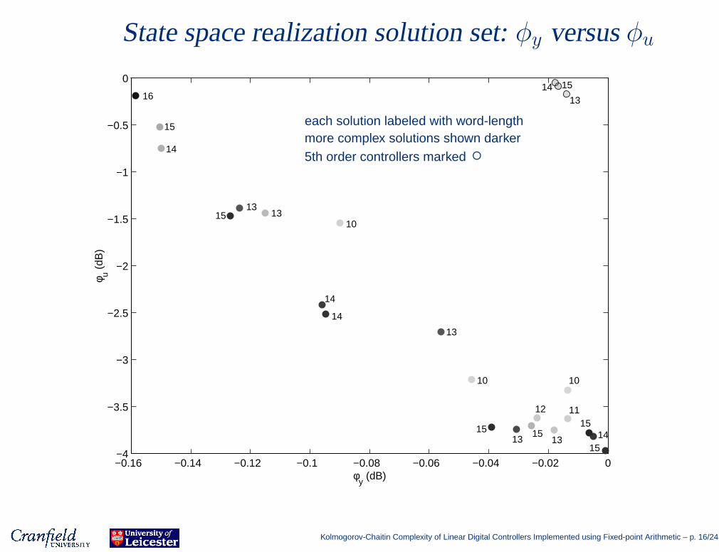
• A set of non-dominated state-space realization controllers that satisfycriteria

φy(Ks) < 0 and φu(Ks) < 0

obtained using Fonseca and Fleming’s multi-objective genetic algorithm• All controllers either 7th order or 5th order with complexity Γ

• We will see that the superiority of the performance of the higher ordercontrollers is clear

• The lower complexity of the lower order controllers is less clear


State space realization solution set: φy versus φu

−0.16 −0.14 −0.12 −0.1 −0.08 −0.06 −0.04 −0.02 0−4

−3.5

−3

−2.5

−2

−1.5

−1

−0.5

0

10

10 10

11

12

13

13

13

13

13

13

14 14

14

14

14

15

15 15

15

15

15

15

16

φy (dB)

φ u (dB

)

each solution labeled with word-lengthmore complex solutions shown darker5th order controllers marked ◦


State space realization solution set: φy versus Γ

−0.16 −0.14 −0.12 −0.1 −0.08 −0.06 −0.04 −0.02 0100

150

200

250

300

350

400

450

500

φy (dB)

Γ5th order controllers marked ⊙


State space realization solution set: φu versus Γ

−4 −3.5 −3 −2.5 −2 −1.5 −1 −0.5 0100

150

200

250

300

350

400

450

500

φu (dB)



Parallel and cascade realization controllers

• Similarly a set of non-dominated parallel and cascade realizationcontrollers are obtained

• All controllers either 7th order or 5th order with complexity Γ

• Again the superiority of the performance of the higher order controllersis clear

• The lower complexity controllers are not necessarily the lower ordercontrollers


Parallel & cascade realization solution set: φy vs φu

−0.16 −0.14 −0.12 −0.1 −0.08 −0.06 −0.04 −0.02 0−4

−3.5

−3

−2.5

−2

−1.5

−1

−0.5

0

10 12

12

12

12

16

16 16

16

20

20

20

20

24

24

24

24

8

φy (dB)

φ u (dB

)

each solution labeled with word-lengthmore complex solutions shown darker5th order controllers marked ◦


Parallel & cascade realization solution set: φy vs Γ

−0.16 −0.14 −0.12 −0.1 −0.08 −0.06 −0.04 −0.02 0100

150

200

250

300

350

400

φy (dB)



Parallel & cascade realization solution set: φu vs Γ

−4 −3.5 −3 −2.5 −2 −1.5 −1 −0.5 0100

150

200

250

300

350

400

φu (dB)



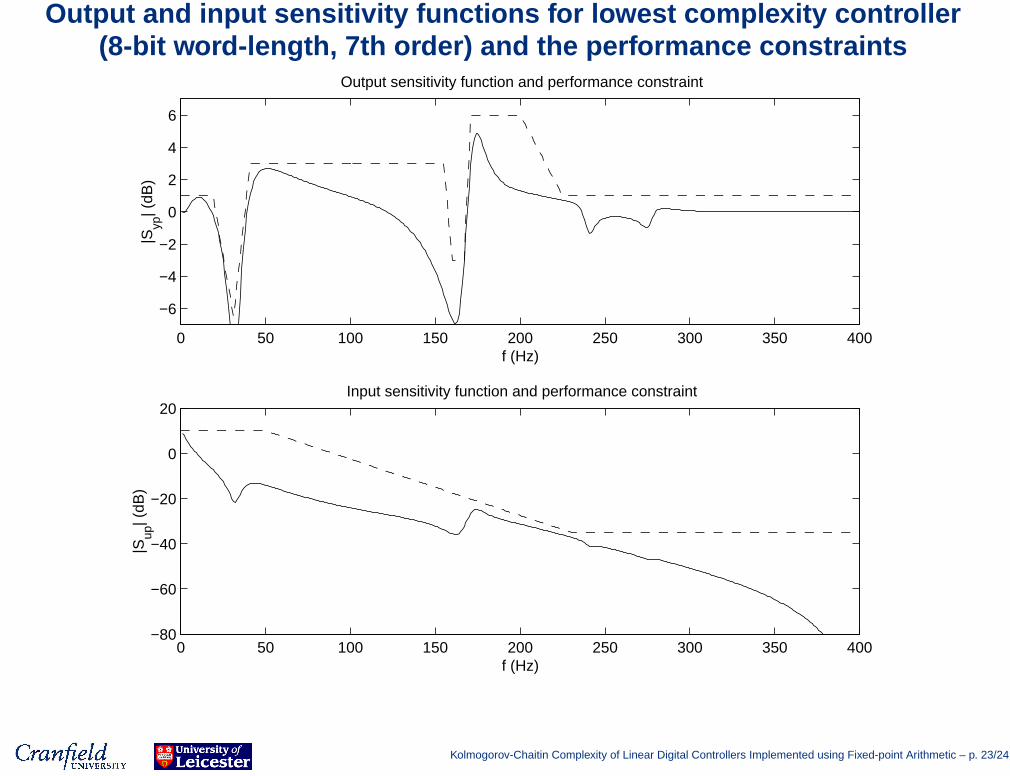
Output and input sensitivity functions for lowest complexity controller(8-bit word-length, 7th order) and the performance constraints

0 50 100 150 200 250 300 350 400

−6

−4

−2

0

2

4

6

f (Hz)

|Syp

| (dB

)

Output sensitivity function and performance constraint

0 50 100 150 200 250 300 350 400−80

−60

−40

−20

0

20

f (Hz)

|Sup

| (dB

)

Input sensitivity function and performance constraint


Conclusions

• We consider controller complexity based on idea of Kolmogorov-Chaitincomplexity

• Practical measures of complexity developed for state-space, parallel andcascade realizations

• Controllers that are low-complexity in this sense will have lowword-length, low number of arithmetic operations and simple realizations— the most important considerations for practical implementations(especially for field-programmable gate arrays)

• Measure is related to the controller order but the lowest complexitycontroller is not necessarily the lowest order

• Higher-order controllers provide an extra degrees of freedom to helpobtain controller realizations that have a shorter word-length and simplerrealization structure, and thus a lower complexity


Date post:	24-Jan-2022
Category:	Documents
Upload:	others
View:	3 times
Download:	0 times

Kolmogorov-Chaitin Complexity of Linear Digital ...

Documents