Chapter .2

k.p Method and a Quantum Dot

In order to predict the electronic and optical properties of semiconductor quantum

dots(QDs) it is necessary to know the electronic band-structure and the wavefunctions for

the valence band(VB) and conduction band(CB). In this chapter we present the theoreti­

cal framework for the computation of electronic states in the VB for a spherical QD. The

electronic states of the CB will be considered in the next chapter. We first present the k.p

theory determining the electronic structure for the bulk semiconductor material;s and then

we show how to apply this theory for the calculation of the elecb'onic structure of a spherical

QD. We present the Hamiltonian for the zinc-blende and wurtzite materials and introduce

the Hilbert space to represent the eigenstates of the VB of the QD. In the next chapter we

present the eigenvalues and eigenfunctions for both the zinc-blende and wurtzite materials

obtained by diagonal zing their respective Hamiltonian in the Hilbert space introduced in

this chapter.

16

2 .1 Introduction

On the way from bulk crystal to quantum dot(QD), it is reasonable to consider the

electrons and holes to feature the properties inherent in an infinite crystal with the finite

size effect of a crystallite depicted as the relevant potential jump at the boundaries. Since

for the most common semiconductors the exciton Bohr radius is much larger than the lattice

constant, a crystallite can be treated as a macroscopic crystal w.r.t. the lattice properties,

but as a quantum box for electrons and holes.

For an infinite ideal crystal a single electron Hamiltonian is given by

_n2

H(r) = -_\72 + V(r) 2me

where V r obeys the translational symmetry of the crystal lattice. The eigenfunctions of the

above Hamiltonian are given by Bloch functions

where unk( r) obeys the same translational symmetry. The wavevector k is determined by

applying the cyclic boundary conditions to the crystal

Ni is the no. of the atoms along the direction ai. We find for k

For a QD Ni f. 00 and finite-size effects determine the envelope function of the eigenfunction.·

For example for a spherical QD with infinite barrier the envelope function of the eigenfunction

vanishes at the boundary.

First we present the theory of the k. p method determining the electronic structure of

the bulk semiconductors and next we show how to apply this method for the calculation of

the electronic structure for spherical QDs.

17

2.2 k.p Methdd ,

2.2.1 Luttinger Kohn Functions

Bloch eigenfunctions of the crystal Hamiltonian are given by

where n labels the band and k takes value in the first Brilloun zone(B.Z) of the crystal. If

one replaces the wavevector k in unk by a constant ko while retaining k in the exponential

factor then the resulting functions

are called Luttinger Kohn functions[60J. These are no longer eigenfunctions of crystal Hamil­

tonian H but they form a complete orthonormali~ed basis set (see Appendix-A). Luttinger

Kohn functions are determined by the Bloch factors unk( f) with k = ko in contrast to the

Bloch functions which require full knowledge of unkU1 for all wavevectors k. Thek.p method

takes advantage of this property of Luttinger-Kohn functions.

2.2.2 Scheme of k.p Method

In this method Schrodinger equation is expressed in terms of Luttinger-Kohn functions.

The resulting matrix elements of H involve the matrix elements of H between the Bloch

factors unk(f) at k = ko only. These elements are just as little known as the Bloch factors

themselves and one takes them as emperical parameters. If one inserts these parameters then

the Hamiltonian matrix in the Luttinger-Kohn basis is completely determined. Diagonalizing

this matrix yields the eigenvalues and eigenfunctions of the crystal Hamiltonian H for all

values of k. This means that the k.p method allows one to calculate the eigenvalues and

eigenfunctions over the entire first Brilloun Zone(BZ) from the Bloch matrix elements at

only one point ko i.e to extrapolate from the particular point ko to the entire first BZ. Often

18

one is only interested in solutions in the vicinity of the valence band maximum(VBM) or

the conduction band minimum(CBM) for which for most semiconductors k = O. Then it

is advantageous, although not necessary, to take ko = O. Taking ko = 0, Luttinger-Kohn

functions are given by InkO >= uno(f)eik.f .

2.2.3 k.p Hamiltonian

The Ansatz[60] ,[61] is

17/J >= L J di2ln'i20 >< n'i2OI7/J > n'

where n' runs over the band index and i2 takes value in the first B.Z of the crystal.

I'¢ >= L J di2 Anl(i2)ln'i20 > n'

Schrodinger Equation is:

HI7/J >= EI7/J >

Taking scalar product with InkO >

L J di2 < nkOIHln'i20 >< n'i2OI7/J >= E < nkOI7/J > n '

L J di2 < nkOIHln'i20 > Anl(i2) = EAn(k) n'

(~\7 ) eik.f uno( f) = (eik.f~ \7 + nk) uno( f)

(~\7 ). (~\7 ) eik.f unk(f) = eik.f[ - n2 \72 + 2~2 (k. \7) + n2 k2] unk(r)

.- - .- _[ n2 \72 n2.... n2

k 2 ] Hu -(r)e~k.r = e~k.r - -- + -. (k.\7) + - + V(f'I uno(f'I

nO 2m zm 2m . J ' J . - ..'

19

..-Using [2~ \12 + V(r)]uno(r) = En(O)UnO(r) where En(O) is the energy at the bottom of the nth

band and -ili\1 = p, the momentum operator, we have

(2.1)

. (2.2)

Only terms with f = k occur in this expansion because of the lattice translational symmetry.

If one defines

with (0).... ,_ . Ii k _ ....

[ 2 2] .

< nOIH (k)ln 0 >- En(O) + 2m tSnn' -In(k)tSnn,

then one obtains from Eq.2.2

< nkOIHln'fO >=< nOIHkp(k)ln'O >

The k dependence of the LK basis on the left has been transferred to the new Hamiltonian

H kp (k) on the right.

The Schrodinger equation with LK basis reads

L < nkOIHln'kO >< n'kOI?/J >= En(k) < nkOI?/J > n'

The Schrodinger equation with the new Hamiltonian reads

L < nOIHkP(k)ln'O >< n'kOI'l/; >= En(k) < nkOI'l/; > n'

wh~re the components < n'kOI'l/; > refer to the LK basis, although the operator Hkp(k) is

represented in Bloch basis InO >. We observe that the matrix representing Hkp(k) is

20

(i) For k = 0 the matrix is diagonal because Hk.p(O) = H(O)(k) .

(ii) For k =1.0 the off diagonal terms are not zero and

-- Ii--< nOIHk.p(k)ln'O >= -k. < nOlfiln'O > . m

Formally one may interpret these non-vanishing elements as arising from an interaction

between different bands. Since this interaction results from the k.p term in Hk.p(k) one

calls it the k.p interaction. Moreover

(iii) As k -+ 0 in Hk.p(k), the k.p interaction tends to zero. For k wavevectors sufficiently

close to k = 0, one can treat this interaction with the help of quantum mechanical pertur-

bation theory.

Hence Hk.p(k) = H(O) + H(l) with

and

2.2.4 Non-Degenerate Energy Bands

I

.:r:

f-Non-degenerate second-order perturbation theory[61] gives the energy, upto second order as

E (k) = OIH(O)1 0 OIH(l)1 0 '"' < nOIH(l)lmO >< mOIH(1)lnO > n < n n > + < n n > + ~ . E (0) _ E (0)

where

mfn n m

li2k2

< nOIH(O)lnO >= En(k) = En(O) + -2m

< nOIH(1)lnO >= 0 since < nOlfilnO >= 0

Ii __ li2

< mOIH(1)lnO >= -k. < mOlfilnO >= -.. klL < mOIVlLlnO > m zm

21

E(k) - (0) h2k

2 _ ~ " "k k < nOI\! /-LImO >< mOI\!"lnO >

n - En + 2m m 2 ~ ~ /-L " E(O) _ B(O) min /-L," n m

Here f-l, v = x, y, z and the so called effective mass tensor m~" is defined by

(2.3)

where

(2.4)

(1) We see that the energy of an electron in a band is very similar to the energy of a free

electron. However, the mass of a band electron is anisotropic and differs from that of a free

electron by a factor determined by the effective mass tensor m~".

(2) The H(l) terms yields exclusively non-diagonal matrix elements and hence it contributes

to the second-order correction to the energy only. Hence the second-order corrections are

needed to obtain an effective mass which differs from the free-electron mass.

2.2.5 Degenerate Energy Bands

In the above section we have considered the special case where the unperturbed energy

levels are non-degenerate. But such a treatment is not sufficient enough as the top of the

VB for most semiconductors is degenerate. Hence in this section we consider the degenerate

perturbation theory[61]. We consider the general case that the unperturbed problem yields

degenerate energy levels each consisting of gn degenerate states InaO > where a = 1,2, ... gn-

The perturbation has two effects.

(1) First its matrix elements between the states characterized by different n modify the states

InaO > in a similar way as described in the non-degenerate theory, so they change them by

22

a small amount into /nak >.

(2) Second, its matrix elements between the states characterized by same n but different

a, lifts part or all of the degeneracy[61]. We include this latter effect by writing the exact

eigenfunctions /7jJ > as linear combinations of the states /nak > with in a multiplet (i.e.

within gn states) gn

/7jJ >= L /nak >< nak/7jJ > a=l

The energy levels E of the full Hamiltonian and the coefficient < nak/7jJ > are solutions of

the matrix equations.

gn

L < nak/H/nbk >< nbk/7jJ >= E < nak/7jJ > b=l

gn

L(Hnk)ab < nbk/7jJ >= E < nak/7jJ > . b=l

while upto second order the matrix elements (Hnk)ab are given by

(H ) - ( )(0) ( )(1) ( )(2) nk ab - H nk ab + H nk ab + H nk ab

where

(HndS'> ~ [<n(O) + ~!218"". (1) Ii - li

2 -

(Hnk)ab = -k. < naO/fi/nbO >= -, kJi < naO/V'J1lnbO > m zm

4 - -(H _/2) = _~ L f < naO/(k.V')/meO >< meO/(k.V')/mbO >

nk ab m 2 m#n c=l ' En(O) - Em (0)

= _ Ii: L L f kJikv < naOIV' Jil meO >< meG/V'vlnbO > m J1.,v m#nc=l En(O) - Em(O)

Hence

(2.5)

23

where j.L, lJ = X, y, Z

(2.6)

and /

(P/l)~b =< naOIV' /lImbO>

Nnw the matrix elements (HniJab are known upto second order, the energy levels E are

obtained up to second order by solving the secular equation of the matrix consisting of these

elements. Thus the energy levels E are the eigenvalues of the gn x gn matrix Hnk with

elements (Hnk)ab and are obtained by solving

det IHnk - Ell = 0 (2.7)

where I is the gn x gn unit matrix with elements 6a,b.

2.2.6 k.p Treatment of the Valence Band

In all the semiconductors the top of the valance band occurs at k = 0, where the

Bloch functions Uno(f) , depicting the crystal periodicity, are the eigenfunctions of crystal

Hamiltonian as well as of H(O). As the VB is made of valence shell orbitals of the atomic

sites, the Bloch wavefunctions at valence band top(VBT) have p-type behaviour and are

3-fold degenerate. The Bloch functions at the VBT are given by

IX >= IvxO >= 6vp (r)x

IY >= IvyO >= 6vp (r)y

IZ >= IvzO >= 6vp (r)z (2.8)

In this case we apply degenerate perturbation theory and hence the energy eigenvalues

are obtained by using Eq.2.7 where the matrix elements (Hnk)7rd of the matrix Hnk are

24

constructed in the basis given in Eq.2.8. Using Eq.2.5 the matrix element (Hnf)7r5 is given

by

(2.9)

where J-L, v = x, y, z and 7r, 8 = X, Y, z.

_1_ = 8 8 _ 21i2 " ~ < n7r0IV J.LlmaO >< maOlVll ln80 > m7r5 7r,5 J.L,II m L L E (0) - E (0) J.LII m#n a=l n m

and < n7r0IV J.Lln80 >= 0 Since the momentum matrix element between two odd functions

is zero the linear term in kJ.L vanishes. Thus, from Eq.2.9, the energy levels in the VB are

the eigenvalues of the matrix

Here the reference of energy has been set as the top of the VB. The symmetry of the diamond

and zinc blende crystal structures requires that the matrix Hnk has the form [60], [40], [61]

where

M- 1 _ 1 _ 1 _ 1 _ 1 _ 1 - mYY - m Zz - mXx - m Zz - mXx - mYY

xx yy yy yy zz zz

N = _1_ = _1_ = _1_ = _1_ = _1_ = _1_ m XY mYZ xZx mY X mZY mXz

xy yz zx yx zy xz

25

(2.10)

(2.11)

(2.12)

= - 2li2 L I: (PxYxr::(Pz);a m m#na=l En(O) - Em(O)

(2.13)

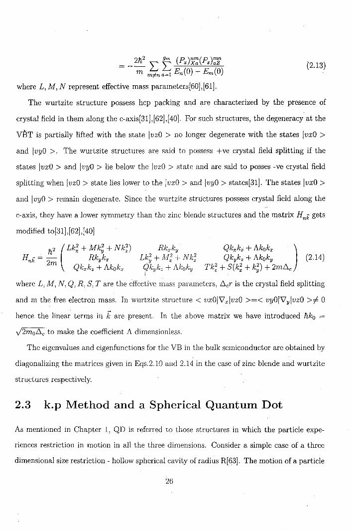
where L, M, N represent effective mass parameters[60]'[61].

The wurtzite structure possess hcp packing and are characterized by the presence of

crystal field in them along the c-axis[31]'[62]'[40]. For such structures, the degeneracy at the

VBT is partially lifted with the state IvzO > no longer degenerate with the states IvxO >

and IvyO >. The wurtzite structures are said to possess +ve crystal field splitting if the

states IvxO > and IvyO > lie below the IvzO > state and are said to posses -ve crystal field

splitting when IvzO > state lies lower to the IvxO > and IvyO > states[31]. The states IvxO >

and IvyO > remain degenerate. Since the wurtzite structures possess crystal field along the

c-axis, they have a lower symmetry than the zinc blende structures and the matrix Hnf gets

modified to[31],[62],[40]

2 (Lk2 + Mk2 + Nk2) li x y z

H f= - Rkykx n 2m

Qkxkz + Akokx (2.14)

where L, M, N, Q, R, 5, T are the effective mass parameters, 6.cT is the crystal field splitting

and m the free electron mass. In wurtzite structure < vxOI'V xlvzO >=< vyOI'V ylvzO >=/= 0

hence the linear terms in k are present. In the above matrix we have introduced liko

J2mo6.c to make the coefficient A dimensionless.

The eigenvalues and eigenfunctions for the VB in the bulk semiconductor are obtained by

diagonalizing the matrices given in Eqs.2.10 and 2.14 in the case of zinc blende and wurtzite

structures respectively.

2.3 k.p Method and a Spherical Quantum Dot

As mentioned in Chapter 1, QD is referred to those structures in which the particle expe-

riences restriction in motion in all the three dimensions. Consider a simple case of a three

dimensional size restriction - hollow spherical cavity of radius R[63]. The motion of a particle

26

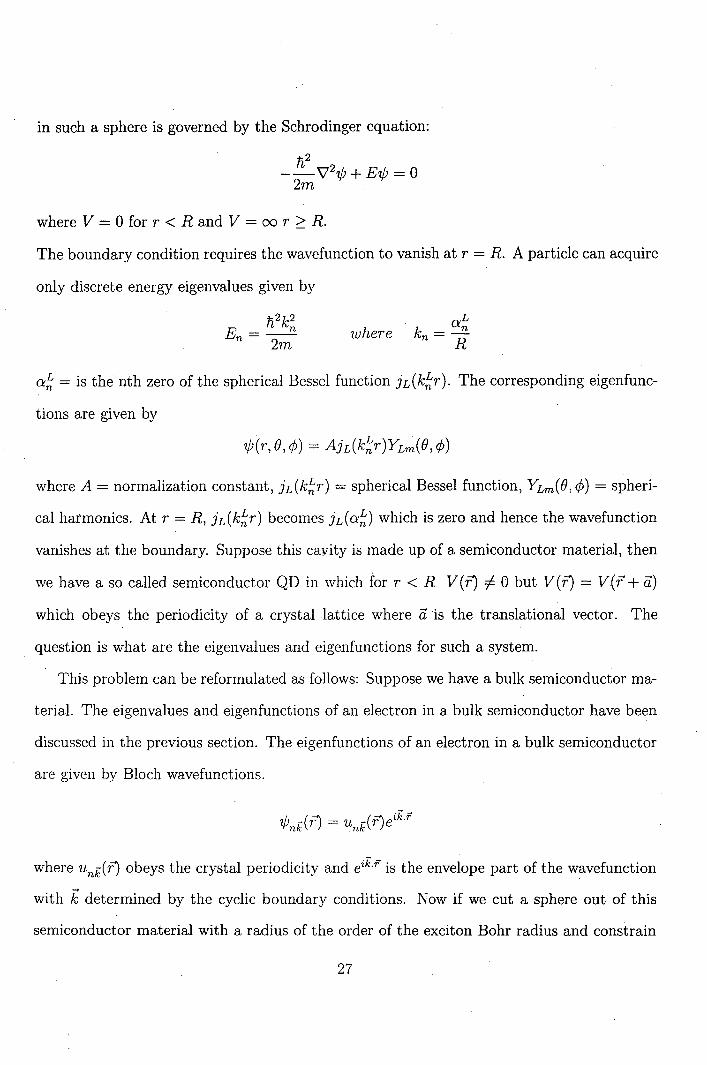
in such a sphere is governed by the Schrodinger equation:

where V = 0 for r < R and V = 00 r 2: R.

The boundary condition requires the wavefunction to vanish at r = R. A particle can acquire

only discrete energy eigenvalues given by

where L

k _ an n- R

a~ = is the nth zero of the spherical Bessel function j L (k~r ). The corresponding eigenfunc-

tions are given by

where A = normalization constant, jdk~r) = spherical Bessel function, YLm(() , ¢) = spheri­

cal harmonics. At r = R, jL(k~r) becomes jL(O:~) which is zero and hence the wavefunction

vanishes at the boundary. Suppose this cavity is made up of a semiconductor material, then

we have a so called semiconductor QD in which for r < R V(f') =I 0 but V(f') = V(f + ii)

which obeys the periodicity of a crystal lattice where iiis the translational vector. The

question is what are the eigenvalues and eigenfunctions for such a system.

This problem can be reformulated as follows: Suppose we have a bulk semiconductor ma-

terial. The eigenvalues and eigenfunctions of an electron in a bulk semiconductor have been

discussed in the previous section. The eigenfunctions of an electron in a bulk semiconductor

are given by Bloch wavefunctions.

where unk( f') obeys the crystal periodicity and eik.r is the envelope part of the wavefunction

with k determined by the cyclic boundary conditions. Now if we cut a sphere out of this

semiconductor material with a radius of the order of the exciton Bohr radius and constrain

27

the motion of the electron to this sphere then the resultant structure formed is a semi-

conductor QD. A semiconductor QD differs from the bulk semiconductor in the boundary

conditions required to be fulfilled by the electron in the two cases. This implies that in a

semiconductor QD the envelope part of the wavefunction is a function of the co-ordinates

r, () and cjJ and the radial part of the wavefunction vanishes at the boundary of the sphere

i.e, at r = R. This indicates that[39],[24]:

(1) The envelope part of the function must be modified by replacing

by L an,L,mjL(k~r)YLm(()' cjJ) n,L,m

where o:~ = k~R are zeros of jL so that the wavefunction vanishes at R.

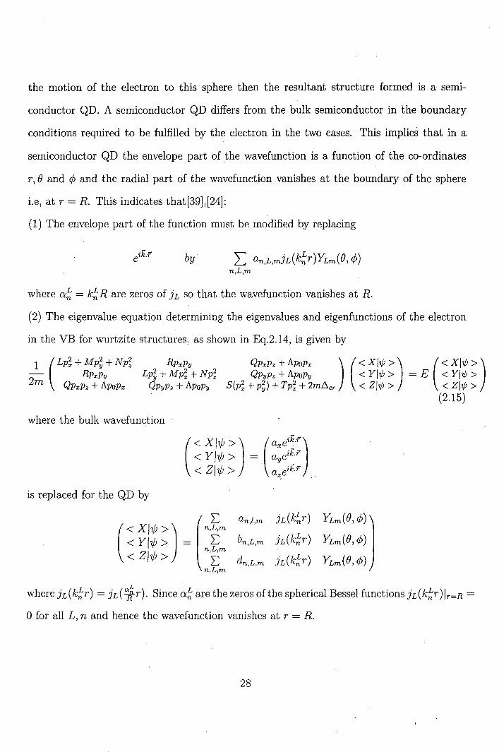
(2) The eigenvalue equation determining the eigenvalues and eigenfunctions of the electron

in the VB for wurtzite structures, as shown in Eq.2.14, is given by

Qpypz + Apopy < Y!7f; > = E < Y!7f; > QpxPz + ApoPx ) « X!7f; » « X!7f; »

S(p~ + p;) + Tp; + 2mllcr < Z!7f; > < Z!7f; >

where the bulk wavefunction

is replaced for the QD by

« XI?jJ »

< YI?jJ > < ZI?jJ >

( < X Iw > ) ( n,F,m < YI?jJ > = L < ZI?jJ > n,~m

n,L,m

(2.15)

an,l,m jL(k~r)

b n,L,m jL(k~r )

dn,L,m jL(k~r)

L where jL(k~r) = jd7f-r). Since o:~ are the zeros of the spherical Bessel functions jL(k~r)lr=R =

o for all L, n and hence the wavefunction vanishes at r = R.

28

2.3.1 Eigenvalue Equation for the Wurtzite and Zinc-Blende Struc­tures

As mentioned earlier, the wurtzite structures have hcp packing. The hexagonal symmetry

gives rise to the presence of the crystal field along the c-axis of the crystal which is absent in

the case of zinc-blende structures. For zinc-blende structures, the spherical approximation for

the Hamiltonian is a good approximation as shown in Appendix-B. Hence for these structures

the eigenvalues and eigenfunctions are obtained by considering the spherically symmetric

Hamiltonian and the states are characterized by a definite value of angular momentum and

its z-component. Since for wurtzite structures crystal field is present along the c-axis, hence

the Hamiltonian is axially symmetric and only the z-component of the angular momentum

is a good quantum number[40).

There are two sources of angular momentum:

(1) L: The orbital angular momentum in a QD is given by spherical harmonics.

(2) I: The Bloch wavefunctions at the VBT uno(f) obeying the crystal periodicity are made up

of p-orbitals coming from atoms making the solid. Hence the Bloch wavefunctions at the VBT

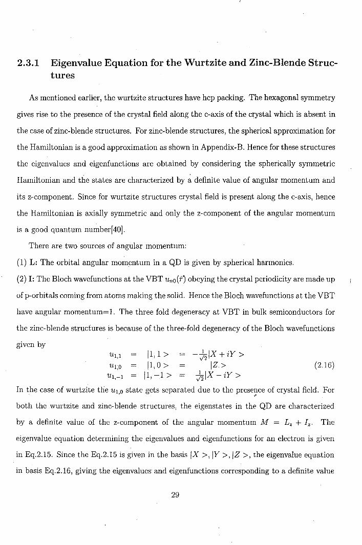
have angular momentum=1. The three fold degeneracy at VBT in bulk semiconductors for

the zinc-blende structures is because of the three-fold degeneracy of the Bloch wavefunctions

given by Ul,l

Ul;O

Ul,-l

11,1> 11,0 >

11,-1 >

-~IX +iY > .J2 IZ>

~IX - iY > .J2

(2.16)

In the case of wurtzite the UIO state gets separated due to the presence of crystal field. For . , ?

both the wurtzite and zinc-blende structures, the eigenstates in the QD are characterized

by a definite value of the z-component of the angular momentum M = Lz + Iz . The

eigenvalue equation determining the eigenvalues and eigenfunctions for an electron is given

in Eq.2.15. Since the Eq.2.15 is given in the basis IX >, IY >, IZ >, the eigenvalue equation

in basis Eq.2.16, giving the eigenvalues and eigenfunctions corresponding to a definite value

29

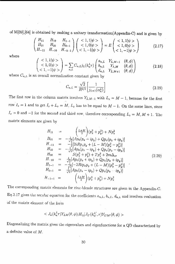
of M[39],[64] is obtained by making a unitary transformation(Appendix-C) and is given by

where

HOI Hoo HO-1 < I, Ol~ > = E < I, Ol~ > ( Hn HlO HI-I) ( < I, 11~ > ) ( < I, 11~ > )

. H-n H_ lO H-1- 1 < I, -11~ > < I, -11~ >

( ~ ~:~I~ ~ ) = LCn,dL(k~r) (~::~ < I, -11~ > n,L dn,L

(0, ¢)) (0, ¢) (0, ¢)

where Cn,L is an overall normalization constant given by

V2 [ 1 1 Cn,L = R3/2 . (L) JL+1 an

(2.17)

(2.18)

(2.19)

The first row in the column matrix involves YL M-1 with Lz = M - I, because for the first ,

row Iz = 1 and to get Iz + Lz = M, Lz has to be equal to M - 1. On the same lines, since

Iz = 0 and -1 for the second and third row, therefore corresponding Lz = M, M + 1. The

matrix elements are given by

H-n HlO Hoo

H_ lO H 1- 1

HO-1

( L~M) (p; + p~) + Np;

- ~[Apo(Px + ipy) + Qpz(px + ipy)] -~[2iRpxpy + (L - M)(p; - p~)]

- ~[Apo(Px - ipy) + QpApx - ipy)] S(p; + p~) + Tp; + 2mL\cr

~[Apo(Px + ipy) + Qpz{px + ipy)]. - ~[-2Ripxpy + (L - M)(p; - p~)] ~[Apo(Px - ipy) + QpApx - ipy)]

( L~M ) (p; + p~) + Np;

(2.20)

The corresponding matrix elements for zinc-blende structures are given in the Appendix-C.

Eq.2.17 gives the secular equation for the coefficients an,L, bn,L, dn,L and involves evaluation

of the matrix element of the form

Diagonalizing the matrix gives the eigenvalues and eigenfunctions for a QD characterized by

a definite value of M.

30

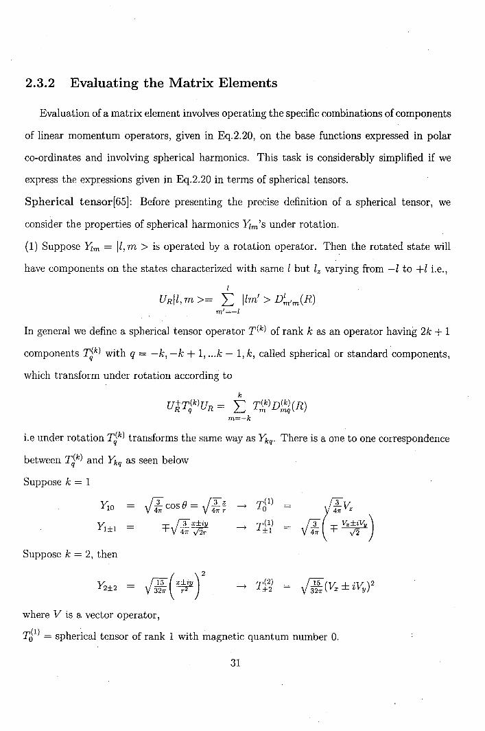
2.3.2 . Evaluating the Matrix Elements

Evaluation of a matrix element involves operating the specific combinations of components

of linear momentum operators, given in Eq.2.20, on the base functions expressed in polar

co-ordinates and involving spherical harmonics. This task is considerably simplified if we

express the expressions given in Eq.2.20 in terms of spherical tensors.

Spherical tensor[65]: Before presenting the precise definition of a spherical tensor, we

consider the properties of spherical harmonics Yim's under rotation.

(1) Suppose Yim = Il, m > is operated by a rotation operator. Then the rotated state will

have components on the states characterized with same l but lz varying from -l to +l Le.,

I

URll, m >= L Ilm' > D~'m(R) m'=-l

In general we define a spherical tensor operator T(k) of rank k as an operator having 2k + 1

components TJk) with q = -k, -k + 1, ... k - 1, k, called spherical or standard ·components,

which transform under rotation according to

k

U+T(k)UR = " T(k) D(k)(R) Rq 0 m mq

m=-k

Le under rotation TJk) transforms the same way as Ykq . There is a one to one correspondence

between T?) and Ykq as seen below

Suppose k = 1

(3 cos e = (3 ~ ---t V4ir V4irr

Suppose k = 2, then

(3 x±iy =r= V 4ir ,;'ir

= fT5(£Eill) 2 V 32:; r2

where V is a vector operator,

T (2) ---t ±2

Td1) = spherical tensor of rank 1 with magnetic quantum number O.

31

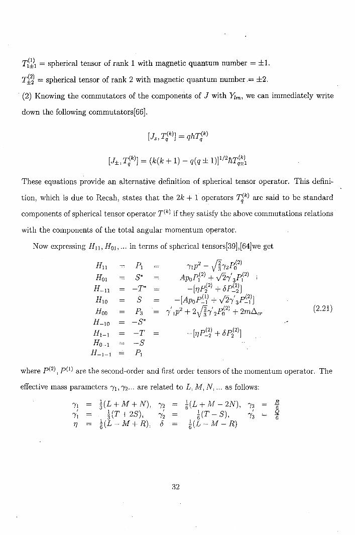
T1(~1 = spherical tensor of rank 1 with magnetic quantum number = ±l.

T~~ = spherical tensor of rank 2 with magnetic quantum number .= ±2.

(2) Knowing the commutators of the components of J with Ylm, we can immediately write

down the following commutators[66].

[J T(k)] = qliT(k) z, q q

These equations provide an alternative definition of spherical tensor operator. This defini­

tion, which is due to Recah, states that the 2k + 1 operators TJk) are said to be standard

components of spherical tensor operator T(k) if they satisfy the above commutations relations'

with the components of the total angular momentum operator.

Now expressing Hll , HOI, ... in terms of spherical tensors[39]'[64]we get

Hll H 'lp2 - if,'2PJ2)

HOI S* ApOPl(2) + V2,' 3P1(2)

H-ll -T* -[17PJ2) + bP~~] HlO S -[Ap p(1) + V2,' p(2)] o -1 3 -1

Hoo P3 '2 if, , (2)

'IP + 2 3' 2PO + 2mt::.cr (2.21 )

H_ 1O -S* r'"

Hl - 1 -T -[1]p~2d + bPJ2)] HO-l -S

H-1- l PI

where p(2), p(1) are the second-order and first order tensors of the momentum operator. The

effective mass parameters ,I, ,2 ... are related to L, M, N, ... as follows:

~ (L + All + N), ,2 HT+2S),

~(L - M + R),

32

~(L+AI-2N), ,3 R

~ (T - S), ,; - ~ ~(L - Ai - R)

We have used the following definition of spherical tensors[67].

with

for rank 0 r,(O)

o for rank 1

TJl)

T (l) ±l

for rank 2 r,(2)

o T (2)

±l T (2)

±2

T12 - T2l

'f ( }, ) [T" - T32 ± i(T31 - T13 )]

j!T33 =t=(T13 ± iT23 )

~(Tll - T22 ± 2iT12 )

\

where the indices i, k = 1,2,3 mean x, y, z respectively and the quantization axis has been

assumed to be the z-axis or 3 axis.

The corresponding matrix elements for the zinc-blende structures are given in Appendix-C.

Now we come l back to the evaluation of the matrix element where the Hamiltonian has

been expressed in terms of spherical tensors

(2.22)

where < L'L~IHijILLz > will involve the evaluation of matrix elements of the form

< L' L~IPJ2)ILLz > where q can be ±2, ±1, O. We have denoted IYLM(B, ¢) > by ILLz > in the

above equations. This expression is evaluated by using the Wigner Eckart Theorem[65],[66].

Wigner Eckart Theorem: The matrix elements of tensor operators with respect to angular

momentum eigenstates satisfy

< L'J..1'IT(k)ILM >= (_l)L'-L < kqLMlkL;L'M' > < L'IIP(2)IIL > q . (2L' + 1)1/2

(2.23)

33

where < kq,LMlkL,L'M' > is the C-G coefficient. < L'IIP(k)IIL > is known as reduced

matrix element and is independent of M, M' and q. Expressed in words, it states that

the matrix elements of the qth component of a tensor operator T(k) between the angular

momentum eigenstates ILM > and IL'M' > equals the product of the C-G coefficient

<kq, LMlkL, L'M' > with a number which is independent of M, M' and q. Hence the

above matrix element has the same selection rules as the C-G coefficient appearing in it i.e

it vanishes unless Ik - LI ::; L' ::; k + L; M' = M + q and IM'I::; L'

In our case k = 2, hence next we consider the evaluation of the reduced matrix element

< L'IIP(2)IIL > From Eq.2.23

< L'M'IP(2)ILM > < L'IIP(2)IIL >= (-1)L-L'(2L' + 1)1/2 q (2.24)

< 2qLMI2L; £I M' >

As mentioned above the reduced matrix element is independent of M, q and M'. Hence

putting M = 0, q = 0, M' = 0, which is simplest to solve [66J ,[68J we get

< L'IIP(2)IIL >= (_l)L-L' (2L' + 1)1/2 < L'OIPJ2)ILO > < 20L012L; £10 >

Evaluating < L'OIPJ2)ILO >

(2.25)

(2.26)

This involves the V' z of the spherical harmonics[68J: < L'OIPzlLO >= -in < L'OIV zlLO >

V'z = cose~ _ sinO ~ dr r dO

(2.27)

It is therefore necessary to evaluate the quanti ties cos OYtm (0, ¢) and sin 0 :fe Yzm (0, ¢ ). The

properties of the legendre functions give[68J

l + 1 l cosOYzo(O, ¢) = [(2l + 1)(2l + 3)]1/2 Yz+1m + [(2l-1)(2l + 1)]1/2 Yz-1,m

. e d (0 ¢) l(l + 1) . y; l(l - 1) sm de ' = [(2l + 1)(2l + 3)]1/2 1+1m - [(2l _ 1)(2l + 1)P/2 Yz-1,m

34

Substituting these in Eq.2.27 reveals that the only non-zero matrix elements of type

< l'OIV zllO > are

. (l + 1) ( d l) < l + 110lVz llO >= [(2l + 1)(2l + 3)]I/2 dr -:;: ¢(r)

l (d l+l) < l- 1iOlVz lLO >= [(2l- 1)(2l + 3)]I/2 dr + -r- ¢(r) (2.28)

Taking the second derivative on the same lines and using the Clebsch-Gordan coefficients we

evaluate Eq.2.25 using 2.26. Some of the reduced matrix elements are listed below[67]. The

rest are given in the Appendix-D.

< L+211P(2)IIL >= ~n2(2(L+2)(L+4))1/2(~ _ 2L+ 1 d + L(L+2)] 2 (2L + 3) dr2 r dr r2

< LIIP(2) ilL >= V3n2 (L(2L + 1)(2L + 2)) 1/2 (~ + ~~ _ L(L + 1)] (2.29) (2L - 1)(2L + 3) dr2 r dr r2

The following important points should be noted: As seen from Eq.2.28, the first derivative

couples L with L + 1 and L - 1. Hence

if IL' - LI =11

The second derivative couples L with L - 2, Land L + 2 only, hence

if I L' - L I =I 0, 2

The above rules make most of the matrix elements as zero.

The matrix element Eq.2.22 becomes

J drr2jL'(k~:r) < L'L~IP?)ILLz > jL(k~r)

= (_I)L1

-L < 2q(~~~~~;)~;;~ > J drr2jL'(k~:r) < L'IIP(2)IIL > jL(k~r) (2.30)

Since pJ2) is a spherical tensor of rank 2 involving components of momentum operator we

come across terms involving radial derivatives of spherical Bessel functions as seen from

35

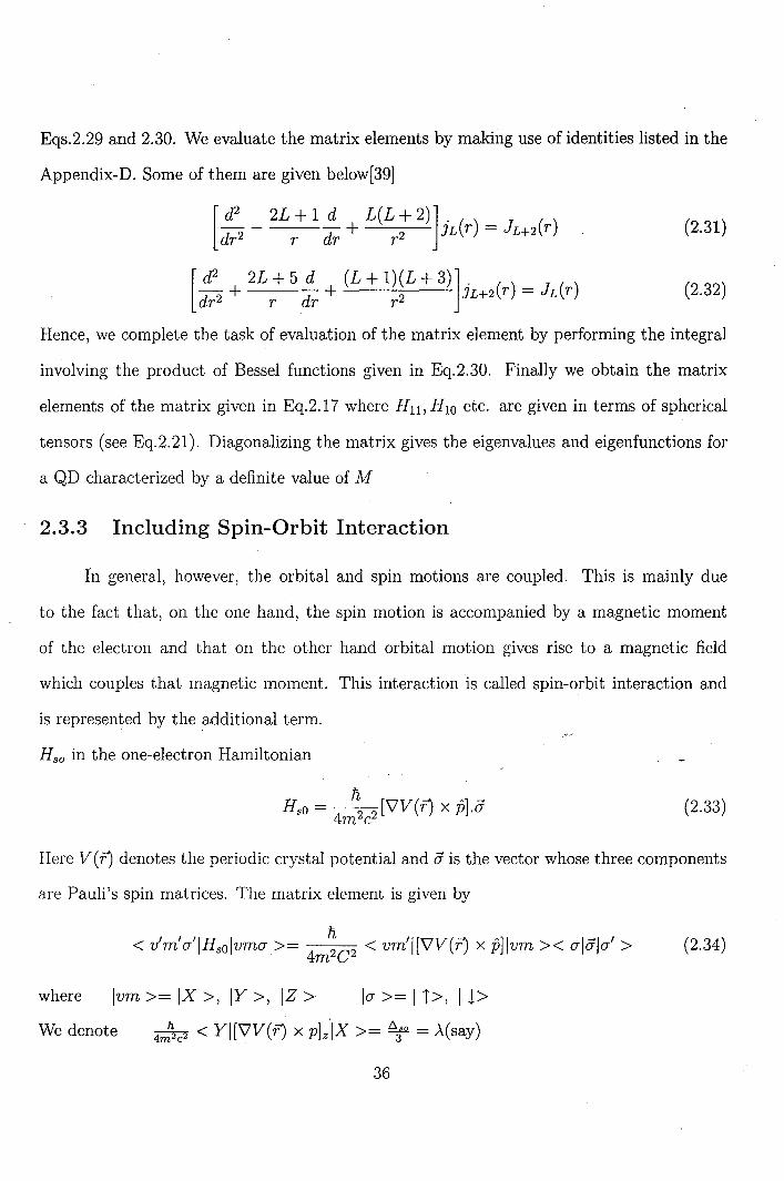
Eqs.2.29 and 2.30. We evaluate the matrix elements by making use of identities listed in the

Appendix-D. Some of them are given below[39]

[ d2 2L + 1 d L(L + 2)]. ( ) _ J () - - - + JL r - L+2 r

dr2 r dr r2 (2.31)

[.!!!.- 2L+5~ (L+1)(L+3)]. ()-J() d 2 + d + 2 JL+2 r - L r r r r r

(2.32)

Hence, we complete the task of evaluation of the matrix element by performing the integral

involving the product of Bessel functions given in Eq.2.30. Finally we obtain the matrix

elements of the matrix given in Eq.2.17 where Hn, HlO etc. are given in terms of spherical

tensors (see Eq.2.21). Diagonalizing the matrix gives the eigenvalues and eigenfunctions for

a QD characterized by a definite value of M

2.3.3 Including Spin-Orbit Interaction

tn general, however, the orbital and spin motions are coupled. This is mainly due

to the fact that, on the one hand, the spin motion is accompanied by a magnetic moment

of the electron and that on the other hand orbital motion gives rise to a magnetic field

which couples that magnetic moment. This interaction is called spin-orbit interaction and

is represented by the additional term.

Hso in the one-electron Hamiltonian

Hso = 4 ~ 2 [VV(f') x p].5 me

(2.33)

Here V (f') denotes the periodic crystal potential and (] is the vector whose three components

are Pauli's spin matrices. The matrix element is given by

< v'm'u'lHsolvmu >= 4m~c2 < vm'I[VV(f') x p]lvm >< ul5lu' > (2.34)

where Ivm >= IX >, IY>, IZ > lu >= I j>, 11>

We denote 4m~c2 < YI[VV(f') x p]zlX >= ~ = .\(say)

36

where tlso is the energy splitting at the VBT due to spin-orbit interaction. To take into

account the spin-orbit interaction the basis is enlarged by taking a direct product of the

earlier basis 11, 1 >, 11,0 >, 11, -1 > defined in Eq.2.16 and the spin eigenstates.

11,1 > I~, ~ > la2> -- 11, 1 > I ~, - ~ > I a5 > -

11, 0 > ~, ~ > la3 > 11,0> ~,-~ > la6 >

11, -1 > I~, t) 11 -1> 11 -- > , 2' 2

The hole Hamiltonian, which is expressed in the above basis is given by

(Ho 0)

H = 0 Ho +Hso (2.35)

where 0 is a 3 x 3 null matrix and Ho is given by Eq.2.17. The explicit expressions of matrix

elements in Ho are given for wurtzite structure in Eq.2.21. and for the zinc. blende structure

in the Appendix-C.

Hso in the above basis is given by[39J,[64]

-,\ 0 0 0 0 0 0 0 0 -J2X 0 0

Hso = 0 0 ,\ 0 -J2X 0

(2.36) 0 -J2X 0 ,\ 0 0 0 0 -J2X 0 0 0 0 0 0 0 0 -,\

Since the evaluation of matrix elements of Ho has already been discussed and the value of I

tlso is available in the data book, the matrix H is completely known. The diagonalization

of the matrix H gives the eigenvalues and eigenvectors characterized by a definite value of

M where M = Lz + Iz + Sz where Sz is the spin projection of the electron.

2.3.4 An alternative Method for Quantum Dots with Zinc-Blende Structure

Hamiltonian matrix in IX >, IY >, IZ > basis is given as

Npxpy Lp~ + M(p~ + p;) (2.37)

Npypz

37

where L, M, N are effective mass parameters. Let us define the three matrices[69]

(0 0 0)

Ix = 0 0 -i o i 0

Iy = ( ~ -i

o i) o 0 o 0

These matrices have the commutation rules of angular momentum i.e

and also satisfy

So they correspond to unit spin. In terms of the matrices just defined we rewrite Eq.2.37.

We have[69]

H = (/1+4/2 )2P2

- 3/2 (p;1;+p;1;+p;1;)- 6

/3 [{Pxpy}{IxIy} + {pypz}{1y1z}+{pzPx}{1zIx}] rno rno 171,0

(2.38)

where {ab} = (ab + ba)/2, rno = free electron mass, p = hole linear momentum operator, ;

j = angular momentum operator. 11, 12, ~/3- are Luttinger parameters defined as

N 13 =--

6

The first term is the particle kinetic energy, and the second and third terms represent a kind

of" 'spin-orbit interaction" [67]. The Hamiltonian in the spherical approximation (Appendix-

B) is given by[67]

Hs h = l [p2 - ~ p( p(2) .1(2))] p 2rno 3

(2.39)

In the strong SOC limit the above Hamiltonian is given by

H - l [p2 - ~ (p(2) )(2))] sph - 2 9· rno

(2.40)

where )(2) and 1(2) are the second-order tensors of angular momentum of 3/2 and 1 respec-

tively. The spherical term

38

can be considered as a kind of" spin-orbit" interaction[67] where the spin operator 8 assumes

the values 3/2 and 1 in the limits of large and small spin-orbit splitting tlso, respectively.

Since the Hamiltonian given in Eqs.2.39, 2.40 are spherically symmetric in the coupled orbital

and spin spaces the total angular momentum F = l + § is a constant of motion. Accordingly

the states can be classified following the L - 8 coupling scheme. We will examplify the

calculation for the strong spin-orbit case. The calculation for the zero SOC case is carried

along the same lines.

In the Hamiltonian (Eq.2.40) the spin-orbit term involves p(2) which as shown in the

previous section couples states satisfying tlL = 0, ±2. Hence there is a parity conservation.

This selection rule, together with the fact that F is a constant of motion, defines the most

general expression for the eigenfunctions [67]of the Hamiltonian (Eqs.2.40) as

n n

where k* R = afv is the nth zero of spherical bessel function jL(k*r). Hence the wavefunction

vanishes at the boundary.

H C - v'2 1 . h 1·· t ere n L - R3/2 J (L) IS t e norma lzatlOn constan . , L+1 aN

/(L, J)F, Lz > are the eigenfunctions of F, in which the orbital angular momentum L is

coupled to angular momentum (J = ~) to obtain F, Fz being the corresponding z-component.

For example

L bnCn,2j2(k~r)/(L = 2, J = ~)F = ~,Fz > n

L gnCn,3j3(k!r)/(L = 3, J = ~F = ~,Fz > n

Here the states are labelled as 83/ 2, H/2 etc. where the subscript gives the value of the total

39

angular momentum and the capital letter denotes the lowest L present. Since the parity is

conserved the first state is an even parity state and second one is an odd parity state.

Substitution of'I/J in the Schrodinger equation with H given by Eq.2.40 leads to secular

equations involving the coefficients an and bn . Evaluation of a matrix element is given in the

Appendix-E. The solution of these equations give the eigenvalues and eigenfunctions of the

hole state in the limit of strong spin-orbit coupling. The eigenvalues and eigenfunctions in

the limit of zero spin-orbit coupling are obtained by doing the calculations on the same lines

. with the role of angular momentum J = ~ being replaced by angular momentum I = 1.

40