54
KPP – A Software Environment for the Simulation of Chemical Kinetics Adrian Sandu Computer Science Department Virginia Tech NIST, May 25, 2004

KPP – A Software Environment for the Simulation of
Chemical Kinetics
Adrian SanduComputer Science Department
Virginia TechNIST, May 25, 2004

May 25, 2004
Acknowledgements
Dr. Valeriu DamianDr. Florian PotraDr. Gregory CarmichaelDr. Dacian DaescuDr. Tianfeng ChaiDr. Mirela Damian
Part of this work is supported by
NSF ITR AP&IM-0205198

May 25, 2004
Related Work
CHEMKIN (http://www.reactiondesign.com/lobby/open) Translates symbolic chemical system in a data file that is then used by internal libraries for simulation. Gas-phase kinetics, surface kinetics, reversible equations, transport, mixing, deposition for different types of reactors, direct sensitivity analysis (Senkin). Database of reaction data, graphical postprocessor for results.
KINALC (http://www.chem.leeds.ac.uk/Combustion/kinalc.htm) Postprocessor to CHEMKIN for sensitivity and uncertainty analysis, parameter estimation, and mechanism reduction; etc.
KINTECUS (http://www.kintecus.com) Compiler/ chemical modeling software. Can run heterogeneous and equilibrium chemistry, generates analytical Jacobians, fit/optimize rate constants, initial concentrations, etc. from data; sensitivity analysis; Excel interface. Can use Chemkin models and databases.
CANTERA (http://rayleigh.cds.caltech.edu/~goodwin/cantera) Object-oriented package for chemically-reacting flows. C++ kernel, STL, standard numerical libraries, Interfaces for MATLAB, Python, C++, and Fortran. Capabilities: homogeneous and heterogeneous kinetics, equilibria, reactor modeling, multicomponent transport.
LARKIN/LIMKIN (http://www.zib.de/nowak/codes/limkin_1.0/full) Simulation of LARge systems of chemical reaktion KINetics and parameter identification. Parser generates Fortran code for function and Jacobian, or internal data arrays.
DYNAFIT (http://www.biokin.com/dynafit) Performs nonlinear least-squares regression of chemical kinetic, enzyme kinetic, or ligand-receptor binding data using experimental data. Parses symbolic equations.

May 25, 2004
KPP in a Nutshell
The Kinetic PreProcessorPurpose: automatically implement building blocks for large-scale simulationsParses chemical mechanismsGenerates Fortran and C code for simulation, and direct and adjoint sensitivity analysisFunction, Jacobian, Hessian, Stoichiometric matrix, derivatives of function&Jacobian w.r.t. rate coefficientsTreatment of sparsityComprehensive library of numerical integratorsUsed in several countries by academia/research/industryFree! http://www.cs.vt.edu/~asandu/Software/KPP

May 25, 2004
KPP Architecture
Fortran C Fortran C
Fortran C Fortran C
Scanner / ParserError checking
Compute best sparsitystructure
Reorder species forbest sparsity
Compute expressiontrees for assignments
Substitutionpre-processor
prod/destr functionjacobian code
sparsity structure
integrator function
driver function(main)
utility functions
I/O functions
Fortran C
Driver file
Integrator file Utility file
I/O file
kinetic description files
atomsspecies
equationsoptions
inline code
KPP
Fortran C
Code generation

May 25, 2004
KPP Example
SUBROUTINE FunVar ( V, R, F, RCT, A_VAR )INCLUDE 'small.h'REAL*8 V(NVAR), R(NRAD), F(NFIX)REAL*8 RCT(NREACT), A_VAR(NVAR)
C A - rate for each equationREAL*8 A(NREACT)
C Computation of equation ratesA(1) = RCT(1)*F(2)A(2) = RCT(2)*V(2)*F(2)A(3) = RCT(3)*V(3)A(4) = RCT(4)*V(2)*V(3)A(5) = RCT(5)*V(3)A(6) = RCT(6)*V(1)*F(1)A(7) = RCT(7)*V(1)*V(3)A(8) = RCT(8)*V(3)*V(4)A(9) = RCT(9)*V(2)*V(5)A(10) = RCT(10)*V(5)
C Aggregate functionA_VAR(1) = A(5)-A(6)-A(7)A_VAR(2) = 2*A(1)-A(2)+A(3)-A(4)+A(6)-
&A(9)+A(10)A_VAR(3) = A(2)-A(3)-A(4)-A(5)-A(7)-A(8)A_VAR(4) = -A(8)+A(9)+A(10)A_VAR(5) = A(8)-A(9)-A(10)RETURNEND
#INCLUDE atoms
#DEFVARO = O; O1D = O; O3 = O + O + O; NO = N + O; NO2 = N + O + O;
#DEFFIXO2 = O + O; M = ignore;
#EQUATIONS { Small Stratospheric }O2 + hv = 2O : 2.6E-10*SUN**3; O + O2 = O3 : 8.0E-17; O3 + hv = O + O2 : 6.1E-04*SUN; O + O3 = 2O2 : 1.5E-15; O3 + hv = O1D + O2 : 1.0E-03*SUN**2; O1D + M = O + M : 7.1E-11; O1D + O3 = 2O2 : 1.2E-10; NO + O3 = NO2 + O2 : 6.0E-15; NO2 + O = NO + O2 : 1.0E-11;
NO2 + hv = NO + O : 1.2E-02*SUN;

May 25, 2004
Sparse Jacobians
1 10 20 30 40 50 60 70 74
1
10
20
30
40
50
60
7074
#JACOBIAN [ ON | OFF | SPARSE ]
IDEAS:• Chem. interactions: sparsity pattern (off-line)• Min. fill-in reordering • Expand sparsity structure• Row compressed form• Doolitle LU factorization• Loop-free substitution
JacVar(…), JacVar_SP(…),JacVar_SP_Vec(…), JacVarTR_SP_Vec(…)
KppDecomp(…)KppSolve(…), KppSolveTR(…)
E.g. SAPRC-9974+5 spc./211 react.NZ=839, NZLU=920

May 25, 2004
Computational Efficiency
8 9 10 20 30 50 80 0.5
1
1.5
2
2.5
3
3.5
4
4.5
5
CPU time [seconds]
Numb
er of
Acc
urate
Digi
ts
qssa
chemeq
vode
sdirk4
rodasS−rodas
S−sdirk4
S−vode
Lsodes
0.120.060.23KPP
0.350.210.61Harwell
Dec+7SolSolDec(1/Lapack)
Linear Algebra
Stiff Integrators

May 25, 2004
Sparse Hessians
#HESSIAN [ ON | OFF ]
kj
ikji yy
fH∂∂
∂=
2
,,
• 3-tensor • sparse coordinate format • account for symmetry
HessVar(…)HessVar_Vec(…)
HessVarTR_Vec(…)
E.g. SAPRC99. NZ = 848x2 (0.2%)

May 25, 2004
Stoichiometric Form
1 20 40 60 80 100 120 140 160 180 200 211
1
20
40
60
79
Reaction
SAPRC−99. Stoichiometric Matrix. NZ = 1024 ( 6 % )
Spe
cies
STOICM (column compressed)ReactantProd(…)
JacVarReactantProd(…)
dFunVar_dRcoeff(…)dJacVar_dRcoeff(…)
#STOICMAT [ ON | OFF ]

May 25, 2004
Requirements for Numerics
Numerical stability (stiff chemistry)Accuracy: medium-low (relerr~10-6-10-2)Low Computational TimeMass BalancePositivity

May 25, 2004
Stiff Integration Methods
( )∑∑=
−
=
− =k
i
innin
k
i
inni yfhy
0
][
0
][ βαBDF
( )
( )j
s
jji
ni
s
jjj
nn
YfayY
Yfbyy
∑
∑
=
=
+
+=
+=
1,
1
1 ,Implicit
Runge-Kutta

May 25, 2004
Rosenbrock Methods
( ) ( ) j
i
jjihii
nh
i
jjji
ni
s
jjj
nn
kcYfkJI
kayY
kmyy
∑
∑
∑
−
=
−
=
=
+
+=⋅−
+=
+=
1
1,
11
1
1,
1
1
γ
No Newton Iterations Suitable for Stiff SystemsMass ConservativeEfficient: Low/Med Accuracy 0.6 0.8 9 1 2 3 4 5 6 7 8 10
0
0.5
1
1.5
2
2.5
3
3.5
4
SEULEX
VODE
Rodas3
Ros3
RODASTWOSTEP
CPU time [seconds]
SD
A

May 25, 2004
Direct Decoupled Sensitivity
( )( ) ( )⎩
⎨⎧
≤≤+⋅=′∂∂==′
mpytfSpytJSpySpytfy
p llll
ll
1,,,,,,
( )[ ]
( )[ ] ⎥⎥⎥
⎦
⎤
⎢⎢⎢
⎣
⎡⋅
⎥⎥⎥⎥⎥
⎦
⎤
⎢⎢⎢⎢⎢
⎣
⎡
+−
+−=ℑ−
⇒=−
−
−
U
U
LPUJJSh
LPUJJShLP
hI
LUPJhI
Tpym
Tpy
T
T
m
L
MOM
L
L
MOM
L
L
0
0
00
000
1
11 1
γ
γγ
γ
Problem

May 25, 2004
DDM with KPP
[ ] ∑
∑−
=
+−++
−
=
+−+
≤≤+=⋅−
+=
1
0
111
1
0
11
1,k
i
np
innn
k
i
ninn
mfhSSJhI
fhyy
llll ββ
β
[ ] ( )
[ ] ( ) ( )
( )∑
∑
∑
∑ ∑∑
−
=
−
=
−
=
=
−
=
+
=
+
++⋅×+⋅++
+⎟⎟⎠
⎞⎜⎜⎝
⎛+⋅=⋅−
++=⋅−
+=+=+=
1
1,
001
1
1
1
1
1
0101
1
1
1
01
1
01
,,,,
,,
,,
i
j
ntpi
nntii
nni
npjijh
iip
i
jjij
niii
nh
i
j
ntijijh
iii
nh
s
i
i
jjij
niii
nns
iii
nn
fhSJhkSHkJkc
pYTfkaSpYTJkJI
fhkcpYTfkJI
kayYkmSSkmyy
ll
l
lll
ll
l
lll
γγ
γ
γ
γ
BDF(Dunker, ’84)
Rosenbrock(Sandu et. al. ‘02)

May 25, 2004
Adjoint Sensitivity Analysis
( ) ( ) ( ))()(,,,' 00 f
yf tytytttytfy ψψ ∇⇒≤≤=
( ) ( ) ( )( ) ( )000)(,,,' ttyttttytJ y
fy
ffT λψψλλλ =∇⇒∇=≥≥⋅−=
Problem: Stiff ODE, scalar functional.
Continuous: Take adjoint of problem, then discretize.
Discrete: Discretize the problem, then take adjoint:
Note: In both approaches the forward solution needs to be precomputed and stored.
( )( ) ( ) ( )( ) ( ) 0
1
0,1,,1,0,
λψψλλ =∇⇒∇=∇=
−==+
Ny
Ny
NkTky
k
kkk
yyyFNkyFy L

May 25, 2004
Linear Multistep Methods
( ) imk
i
imiim
mTk
i
imimi hyJ +
=
++
=
++ ∑∑ ⋅= λβλα0
][
0
][
( )∑∑=
−
=
− =k
i
innin
k
i
inni yfhy
0
][
0
][ βαMethod
Continuous Adjoint
Discrete Adjoint
( ) imk
i
imTmim
k
i
immi yJh +
=
+
=
+ ⋅= ∑∑ λβλα0
][
0
][
Consistency: ~one-leg method, in general not consistent with continuous adj. eqn.Implementation: with KPP
May 25, 2004
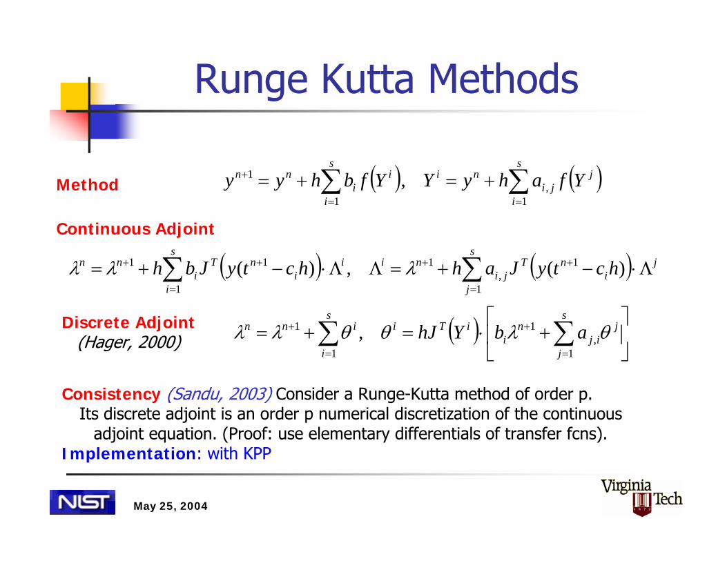
Runge Kutta Methods
( ) ⎥⎦
⎤⎢⎣
⎡+⋅=+= ∑∑
=
+
=
+s
j
jij
ni
iTis
i
inn abYhJ1
,1
1
1 , θλθθλλ
( ) ( )∑∑==
+ +=+=s
i
jji
nis
i
ii
nn YfahyYYfbhyy1
,1
1 ,Method
Continuous Adjoint
Discrete Adjoint(Hager, 2000)
( ) ( ) ji
nTs
jji
niii
nTs
ii
nn hctyJahhctyJbh Λ⋅−+=ΛΛ⋅−+= +
=
++
=
+ ∑∑ )(,)( 1
1,
11
1
1 λλλ
Consistency (Sandu, 2003) Consider a Runge-Kutta method of order p. Its discrete adjoint is an order p numerical discretization of the continuous
adjoint equation. (Proof: use elementary differentials of transfer fcns).Implementation: with KPP

May 25, 2004
Singular Perturbation
(Sandu, 2003)If RK with invertible coefficient matrix A and R(∞) = 0;
and the cost function depends only on the non-stiff variable yThen µ= 0 and λ are solved with the same accuracy as the original
method, within O(ε).A similar conclusion holds for continuous RK adjoints.
ftttzygzzyfy ≤≤== 0),,('),,(' ε
( ) ( ))(),()(,)(),()( )()(ff
tzff
ty tztyttztyt ψµψλ ∇=∇=
Test problem relevant for stiff systems:
Distinguish between derivatives w.r.t. stiff/non-stiff variables

May 25, 2004
Rosenbrock Methods
( )[ ] ( )
( )
( ) ∑∑
∑
==
+
+=
+
+⋅×+=
≥≥⋅=
++=⋅−
s
iii
s
i
Ti
nnn
iiT
i
s
ijjijhjij
nii
Tnh
vukH
isuYJv
ucvamuJI
11
1
1,
1,
11
1
λλ
λγ
( )[ ] ( ) sizcYJzJI
zmhtyYza
jji
i
jh
iiTi
Tnh
j
s
jj
nni
ji
nijji
ni
≤≤+Λ⋅=⋅−
+=−=+=Λ
∑
∑∑−
=
+
=
+−
=
++
1,
,)(,
,
1
1
111
1
11
1
1,
1
γ
λλαλ
DiscreteAdjoint
ContinuousAdjoint
Consistency (Sandu, 2003) Similar to Runge-KuttaImplementation: with KPP

May 25, 2004
Computational Efficiency
Tdiscrete adjoint≤ 5 Tforward (Griewank, 2000)KPP/Rodas-3 on SAPRC-99:
4.42.33.31.2
Tdiscr-grad
/Tfwd
Tdiscr-adj
/Tfwd
Tcont-grad /Tfwd
Tcont-adj
/Tfwd

May 25, 2004
KPP Numerical Library
SimulationSparse: BDF (VODE, LSODES), Runge-Kutta(Radau5), Rosenbrock (Ros-{1,2,3,4},Rodas-{3,5}. QSSA. DriversDirect Decoupled SensitivitySparse: ODESSA, Rosenbrock, I.C. and R.C.Adjoint SensitivityContinuous Adj. with any simulation methodDiscrete Adj. Rosenbrock. Drivers.

May 25, 2004
Max Planck Institute

May 25, 2004
MISTRA-MPIC, U. Heidelberg
“Chemical reactions in the gas phase are considered in all model layers, aerosol chemistry only in layers where the relative humidity is greater than the crystallization humidity. […] The set of chemical reactions is solved using KPP.”
(http://www.iup.uni-heidelberg.de/institut/forschung/groups/atmosphere/modell/glasow)

May 25, 2004
User Contributions to KPP
Artenum SARLParisCyberVillage
101-103 Bld Mac Donald75019 Paris 19ème
France www.artenum.com
(Consulting company)

May 25, 2004
Example: Modeling Air Pollution

May 25, 2004
The Forward Model
( ) ( )
( ) ( )( ) ( )
GROUNDii
DEPi
i
OUTi
ININii
Fii
iiiii
onQCVnCK
onnCK
onxtCxtC
tttxCxtC
ECfCKCudt
dC
Γ−=∂∂
Γ=∂∂
Γ=
≤≤=
++∇⋅∇+∇⋅−=
0
,,
,,
11
000
ρρ
ρρ
r
Mass Balance Equations. C = mole fraction. ρ = air density.

May 25, 2004
Discrete Forward Model
tHOR
tVERT
tCHEM
tVERT
tHORttt
kttt
k
TTRTTN
CNC∆∆∆∆∆
∆+
∆++
=
=
oooo
o
],[
],[1
Operator Splitting:Conservative Methods for TransportStiff Methods for Chemistry (KPP), Specific Methods for Aerosols,Different Time Steps.

May 25, 2004
Chemical Data Assimilation
��������������������������������������������������������������������������������������������������������������������������������������������������������������������������������������������������������������������������������������������������������������������������������������������������������������������������������������������������������������������������������������������
��������������������������������������������������������������������������������������������������������������������������������������������������������������������������������������������������������������������������������������������������������������������������������������������������������������������������������������������������������������������������������������������
e.g. clouds, winds.ofthe atmosphere
Physical aspects
and optical propertieschemical components
destruction of the
evolution, including(CTMs) provide the
production and provide
Chemical ModelsMeteorologicalModels
Atmospheric Models
New Approaches
Assimilation Techniques:
Improved repre−
transport features
Chemical & OpticalObservations:
Sattelite, ground, aircraftColumn (integral) quantities
Algorithms
BetterRetrieval
Meteorological Observations
Winds, Temperature, Clouds
sentation of
cloud fluxes
Emission Estimates
Adjoint Modeling
Variational (4D−Var)
Fluxes BudgetsConcentrations
Model Outputs:
Optimal Analysis State
analysis fieldsassimilated forecasts;
MeteorologicalImproved
for Improved
Inverse Modeling
Emission Estimates
measurement strategiesModel Performance;
FeedbacksApplications
Better designof observation networks/
weather forecasts
and Chemical
Improved Air Quality
Evaluation;
May 25, 2004
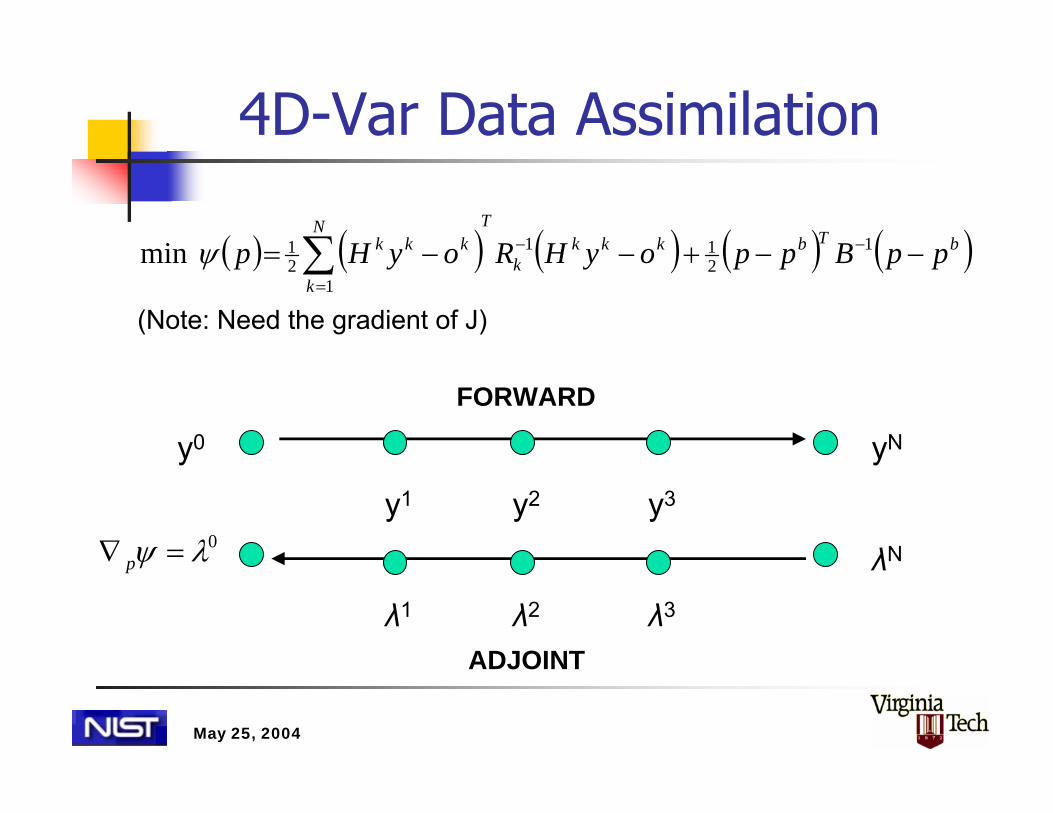
4D-Var Data Assimilation
( ) ( ) ( ) ( ) ( )bTbkkkk
TN
k
kkk ppBppoyHRoyHp −−+−−= −−
=∑ 1
211
121min ψ
y0 yN
FORWARD
ADJOINT
λN
y1 y2 y3
λ1 λ2 λ3
(Note: Need the gradient of J)
0λψ =∇ p

May 25, 2004
Continuous Adjoint Model
( ) ( )
( ) ( )( )
( )
( ) GROUNDi
DEPi
i
OUTii
INi
oFFi
Fi
iiTi
ii
onVn
K
onn
Ku
onxt
tttxxt
CFKudtd
Γ=∂
∂
Γ=∂
∂+
Γ=
≥≥=
−⋅−⎟⎟⎠
⎞⎜⎜⎝
⎛∇⋅⋅∇−⋅∇−=
λρλρ
ρλρλ
λ
λλ
φλρρλρλλ
0
0,
,,
)(
r
r
Note: Linearized chemistry generated by KPP.

May 25, 2004
Discrete Adjoint Model
( ) ( ) ( ) ( ) ( )
( ) ( ) ( ) ( ) ( )'*'*'*'*'*],[
'*
1],[
'*
'''''],[
],[1
tHOR
tVERT
tCHEM
tVERT
tHORttt
kttt
k
tHOR
tVERT
tCHEM
tVERT
tHORttt
kttt
k
TTRTTN
N
TTRTTN
CNC
∆∆∆∆∆∆+
+∆+
∆∆∆∆∆∆+
∆++
=
=
=′
′=
oooo
o
oooo
o
λλ
δδ
Operator Split Tangent Linear and Adjoint Discrete Models
Note: Chemical Model Discrete/Continuous Adjoints automatically generated by KPP

May 25, 2004
Adjoint STEM-IIIMeasurement info used to adjust initial fields and improve predictions;
East Asia. Grid: 80 x 80Km. Time: [0,6] GMT, 03/01/01.
SAPRC 99 (Ros-2); 3rd order upwind FD; LBFGS;
Parallelization with PAQMSG
Distributed Level-2 Checkpointing Scheme
I/O Data
Local Chkpt Local Chkpt Local Chkpt Local Chkpt
Node NodeNode Node
Master
0 5 10 15 200
5
10
15
20
No. Workers
Rel
ativ
e Sp
eedu
p
Ideal SpeedupRelative Speedup

May 25, 2004
NASA Trace-P Experiment
Transport and Chemical Evolution over the Pacific
March-April 2001
Quantify Asian transport
Understand chemistry over West Pacific

May 25, 2004
Computational domain:• Area: 7.200 x 4.800 km• Horizontal grid: 80 x 80 Km• Vertical grid: 18 layers,10 km.
Computational Setting
Model Size ~ 8,000,000 variables

May 25, 2004
Trace-P Simulation
March 01-04, 2001O3 NO2SO2

May 25, 2004
Model vs. Observations
10
20
30
40
50
60
70
80
90
24 25 26 27 28 29 30 31 32 330
2000
4000
6000
8000
10000
12000
O3
(ppb
v)
Alti
tude
(m
)
TIME (GMT)
Observed O3 Modeling O3
Flight Height (m)
Modeled O3 vs. Measured O3
• Cost functional =model-observation gap.
• The analysis produces an optimal state of the atmosphere using:
Model information consistent with physics/chemistry
Measurement information consistent with reality

May 25, 2004
More Observations
0
0.02
0.04
0.06
0.08
0.1
0.12
0.14
0.16
0.18
0.2
24 25 26 27 28 29 30 31 32 330
2000
4000
6000
8000
10000
12000
NO
(p
pb
v)
Alti
tud
e (
m)
TIME (GMT)
DC-8 Flight #6 NO on 3/3/2001
Observed NO Modeling NO
Flight Height (m)
0
0.5
1
1.5
2
2.5
3
3.5
4
24 25 26 27 28 29 30 31 32 330
2000
4000
6000
8000
10000
12000
SO
2 (
ppbv)
Alti
tude (
m)
TIME (GMT)
DC-8 Flight #6 SO2 on 3/3/2001
Observed SO2 Modeling SO2
Flight Height (m)
NO: Observation vs. Model SO2: Observation vs. Model

May 25, 2004
Target: O3 at Cheju Island
March 4-6, 2001: Strong NE flow, Beijing-Cheju
March 22-25, 2001:Weaker Flow

May 25, 2004
Cones of Influence
March 4-6, 2001 March 22-25, 2001
O3
NO2
HCHO
Isosurfaces of time integrals of adjoint vars. (ψ = O3 at Cheju).

May 25, 2004
Areas of InfluenceΨ = Ozone at Cheju, 0GMT, 03/04/2001Influence areas (adjoint isosurfaces) depend on meteo, but
cannot be determined solely by them (nonlinear chemistry).Boundary condition uncertainties 3 days before.
d ψ / d O3 d ψ / d HCHO d ψ / d NO2
May 25, 2004
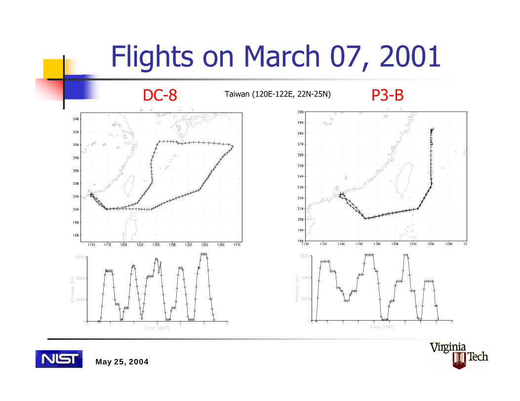
Flights on March 07, 2001DC-8 P3-BTaiwan (120E-122E, 22N-25N)
May 25, 2004
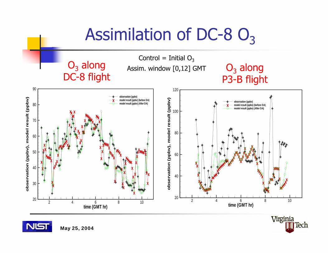
Assimilation of DC-8 O3
+
+
+
+
+
+
++
+++
+
+
+
+++
+
+++
+
++
+++
+
++
++
++
+++
++++
++
++++++
+++
+++
+++++++
+
++
++++++
+++
+++
+
++++++
+
+
++
++++++++++
++
+
+++++++
+
+
+
+
xx
xxxxxxxxx
xx
xxxxxxxxxxx
xxxxx
x
xxxxx
xxxxx
xx
xxx
xxxxxxxxx
xxx
xxxx
x
xxxxxxxxx
xxxxx
x
x
xxxxx
x
xx
x
xxxxxxx
x
x
x
x
xxxxxxxxxxx
x
x
x
time (GMT hr)
ob
se
rva
tio
n(p
pb
v),
mo
de
lre
su
lt(p
pb
v)
2 4 6 8 1020
30
40
50
60
70
80
90
observation (ppbv)model result (ppbv) (before DA)model result (ppbv) (After DA)
+x
Control = Initial O3
Assim. window [0,12] GMT
+
+
+
+
++
++
+
+++
++
+
+
+
+
+++
++
+++++
+++
+
++++
++++++
+++
+++
+
++++++++++++
+
+++
+
+
+++++
+
++
+
+++++
+
+
+
++++++
xx
xxxxxxxxxxxxx
xxxxx
xxxx
xxxxxxxxxxx
xxxxxxxxxxx
xxxxxx
xxxxx
xxxxxxxxx
xxxxxx
xxxx
xxxxxx
x
xxxxxxx
time (GMT hr)
ob
se
rva
tio
n(p
pb
v),
mo
de
lre
su
lt(p
pb
v)
2 4 6 8 1020
40
60
80
100
120
observation (ppbv)model result (ppbv) (before DA)model result (ppbv) (After DA)
+x
O3 alongP3-B flight
O3 along DC-8 flight

May 25, 2004
Assimilation of P3-B O3
Control = Initial O3Assim. Window [0,12] GMT
O3 alongP3-B flight
O3 along DC-8 flight
+
+
+
+
++
++
+
+++
++
+
+
+
+
+++
++
+++++
+++
+
++++
++++++
+++
+++
+
++++++++++++
+
+++
+
+
+++++
+
++
+
+++++
+
+
+
++++++
xx
xxxxxxxxxxxxx
xxxxx
xxxx
xxxxxxxxxxx
xxxxxxxxxxx
xxxxxx
xxxxx
xxxxxxxxx
xxxxxx
xxxx
xxxxxx
x
xxxxxxx
time (GMT hr)
ob
se
rva
tio
n(p
pb
v),
mo
de
lre
su
lt(p
pb
v)
2 4 6 8 1020
40
60
80
100
120
observation (ppbv)model result (ppbv) (before DA)model result (ppbv) (After DA)
+x
+
+
+
+
+
++++++
++
+
+++
+
+++
+
++
+++
+
++
+++++++
++++
++
++++++
++++++
+++++++
+
++
++++++
++++++
+
++++++
+
+++
++++++++++
++
+
+++++++
+
+
+
+
xx
xxxxxxxxx
xx
xxxxxxxxxxx
xxxxx
x
xxxxx
xxxxx
xx
xxx
xxxxxxxxx
xxx
xxxx
x
xxxxxxxxx
xxxxx
x
x
xxxxx
x
xx
x
xxxxxxx
xx
x
x
xxxxxxxxxxx
x
x
x
time (GMT hr)
ob
se
rva
tio
n(p
pb
v),
mo
de
lre
su
lt(p
pb
v)
2 4 6 8 1020
40
60
80
100
observation (ppbv)model result (ppbv) (before DA)model result (ppbv) (After DA)
+x

May 25, 2004
Assimilation of Multiple SpeciesP3-B Obs: O3(8%); NO, NO2(20%); HNO3, PAN, RNO3(100%)
+
+
+
+
++
+
+
+
+++
++
+
+
+
+
+++
++
+++++
+++
+
++++
++++++
+++
+++
+
++++++++++
++
+
+++
+
+
+++++
+
++
+
+++++
+
+
+
++++++
XX
XXXXXXXXXXXXX
XXXXX
XXX
XXXXXX
XXXXXX
XXXXXXXXXXX
XXXXXXX
XXXXXXXXXXXXX
XXXXXX
XXXX
XXXXXX
X
XXXXXXXX
X
X
Time GMT (hr)
O3
4 6 8 1020
40
60
80
100
120
++++++
++++++++++++
+++++++++
++++++
++
++++
+++++
+++++++++++
++
+
++++
+++++++
+++++++++
++++
+++
+XXXXXXXXXXXXXXXXXXXXXXXXX
XXXXXXXXXXXXXXXXXXX
X
XX
X
XXXX
X
X
XX
X
X
X
X
XXXXXXXXXXXXXXXXXXXXXX
XXXXXXXXXX
X
Time GMT (hr)
RNO3
4 6 8 100
0.02
0.04
0.06
0.08
0.1
0.12
+
+
++++
+++++++++
+
+
+++
++++
++
+
+
+++
+++++
+
+++
+
+
+
+
+++
+
++++++++++
++
+
++++++++++
+
+++
+++++++++++
+
+
+
+
+XXX
XXXXXXXXXXXXXXXXXXXX
XXXXXXXX
XXXXXX
XXXXXXX
X
XX
X
X
X
XXXXXX
X
X
X
XXXXXXXXXXXXXXXXXX
XXXXXXXXXXXXXXX
X
Time GMT (hr)
PAN
4 6 8 100
0.2
0.4
0.6
0.8
1
1.2
+++++
+++++++++
+
++++
+++++
++++++++++
+++++++++
+++++
++++++
+
+
+XX
X
XXXXXXXXXXXXXXXXX
X
XXXXXXXXX
X
XXXXXXXXXXXXXXXXX
X
X
XXXXXXXX
XX
XXXXXXXXXXXX
XXXXXXXXX
XX
XXXXXXXX
X
X
Time GMT (hr)
HNO3
4 6 8 100
0.5
1
1.5
2
+
++
+ +
+
+++
+++++++
+++++++++
+++++
+++++
+
+
+
++
+
+++++
+++
++
+
+++++++
+
+
+
XXXXXXXXXXXXXXXXXXX
XXXXXXXXXX
XX
XXXXXXXXXXXXXXXXX
X
X
XXXXXX
X
X
X
XXXXXXXXXXXX
XXXXX
X
XX
X
X
XXXXXXXX
X
X
Time GMT (hr)
NO2
4 6 8 100
0.1
0.2
0.3
0.4
+
+
+
+++++++++
++++
+
++++
++++++++++
+
+++++
+
++++
+
+++++
+
++
+
+++++
+++++
+
+++
++
+
++
+++++++
+++
X
XXXXXXXXXXXXX
XXXXXXXXXXXXXXXX
X
XXXXXXXXXXXXXXXXXXXXXXXXXXXX
XXXXXXXXXXXX
XXXXXXXXX
XXXXXXXXXX
X
X
Time GMT (hr)
NO
4 6 8 100
0.02
0.04
0.06
0.08
0.1
0.12
0.14
O3
NO2
PAN
NO
HNO3
RNO3

May 25, 2004
Sensitivity AnalysisVe
rtica
lleve
l
0 5 10 15 20 25 30 35 40 45 50 55 60 65
5
10
15
1E-09 1E-08 1E-07 1E-06 1E-05 0.0001 0.001 0.01
Species Index
1. O32. H2O23. NO4. NO25. NO36. N2O57. HONO8. HNO39. HNO410. SO2
11. H2SO412. CO13. HCHO14. CCHO15. RCHO16. ACET17. MEK18. HCOOH19. MEOH20. ETOH
51. PHEN52. PAN53. PAN254. PBZN55. MA_PAN56. BC57. OC58. SSF59. SSC60. OPM10
41. ALK342. ALK443. ALK544. ARO145. ARO246. OLE147. OLE248. TERP49. RNO350. NPHE
31. PROD232. DCB133. DCB234. DCB335. ETHENE36. ISOPRENE37. C2H638. C3H839. C2H240. C3H6
21. CCO_OH22. RCO_OH23. GLY24. MGLY25. BACL26. CRES27. BALD28. ISOPROD29. METHACRO30. MVK
61. OPM2562. DUST163. DUST264. DUST365. DMS66. CO2
Sensitivity magnitude
ψ = NOY (P3-B)Averaged gradients help with choice of control variables

May 25, 2004
Assimilation of DC-8 CO
Control: Initial Conc. of 50 spc.
+
+
+++++++++++
++++
++
++
+
++++
+
+++++
+
++
+
+
+
++
+
+
++
++++
++
+
+++++++++
++
+
++++++++++
++++++++++++
++++++++
+++++++++++++
++++
+
+XX
XXXXXXXXXXX
X
XXXX
XXXXX
XXXX
X
X
X
XXXXX
X
X
XX
X
X
XX
XX
X
X
XXXXXXX
XXXX
XXXX
X
X
X
XXXXXXXXXXXX
XXXXXXXX
XX
X
XXXXXXXX
X
XXXXXXXXXXXX
XX
X
X
XX
Time (GMT hr)
CO
con
cetr
atio
ns
(pp
bv)
0 2 4 6 8 10 120
50
100
150
200
250
300
350
400
ObservationsModel (before DA)Model (after 10 iterations)
+X
+
+
++++
+++++++
++++
++
++
+
++++
+
+++++
+
++
+
+
+
++
+
+
++
++++
++
+
+++++++++
++
+
++++++++++
++++++++++++
++++++++
+++++++++++++
++++
+
+XX
XXXXXXXXXX
X
XXXX
XXXXX
XXX
X
X
XXXXX
X
X
XX
X
X
XX
XX
X
X
XXXXXXX
XXXX
XXXX
X
X
X
XXXXXXXXXXXX
XXXXXXXXX
XX
XXXXXXXX
X
XXXXXXXXXXXXX
XX
X
XX
Time (GMT hr)CO
Ob
serv
atio
n(p
pb
v),C
Om
od
elp
red
ictio
n(p
pb
v)
2 4 6 8 100
50
100
150
200
250
300
350
400CO Observation (ppbv)CO model prediction (ppbv) (before DA)CO model prediction (ppbv) (after 4 iterations)
+X
Control: Initial CO Conc.

May 25, 2004
Assimilation of DC-8 COControl:
Initial Conc. 50 spc. CO alongP3-B flight
CO along DC-8 flight
+
+
+++++++++++
++++
++
++
+
++++
+
+++++
+
++
+
+
+
++
+
+
++
++++
++
+
+++++++++
++
+
++++++++++
++++++++++++
++++++++
+++++++++++++
++++
+
+XX
XXXXXXXXXXX
X
XXXX
XXXXX
XXXX
X
X
X
XXXXX
X
X
XX
X
X
XX
XX
X
X
XXXXXXX
XXXX
XXXX
X
X
X
XXXXXXXXXXXX
XXXXXXXX
XX
X
XXXXXXXX
X
XXXXXXXXXXXX
XX
X
X
XX
Time (GMT hr)
CO
conc
etra
tions
(ppb
v)
0 2 4 6 8 10 120
50
100
150
200
250
300
350
400
ObservationsModel (before DA)Model (after 10 iterations)
+X
++
+
+++++++++++++
+
+
++
+
++
++
+++
+++
+
+++++
+
++++
++
+
+++
++++++
+++
++
+
++
+++
+++++++
+
+++
++++++
+
+++++
+
+
+
+X
X
X
XXXXXXXXX
XXX
XXXXXX
XXXXX
X
XXXX
XX
X
X
XX
XXXX
XXX
X
XX
XX
X
X
X
X
X
XX
X
X
X
X
XX
XXXX
X
XXXXX
XXXX
X
XXXXX
X
XXXXX
X
X
XXX
Time (GMT hr)
CO
conc
etra
tions
(ppb
v)
2 4 6 8 100
50
100
150
200
250
300
350
400
450
p3 ObservationsModel (before DA)Model (after 10 iterations)
+X

May 25, 2004
Different Control Sets
++
+
++++++
+++++++
+
+
+++
+++++
++
+++
+
++++
+++++
+
++++++
+
+++++++
+++
++
+
++++++++++
+
+++
+++
+++
+
++++++
+
+
+
+
X
X
X
XXXXXXXXXXXXXXXXX
X
XXXXX
XXXXXX
XXXXX
XXXXXXX
X
XX
X
XX
XXXXXX
X
X
XXXX
XXXX
X
XXXXXXXX
XX
XXXXX
X
XXXXXXX
X
X
X
TIME (GMT hr)
NO
y(p
pb
v)
2 4 6 8 100
0.5
1
1.5
2
2.5
3
3.5
4
4.5
ObservationModel (Without 4D-Var)Model (Ctrls: NO + NO2 + HNO3 + PAN +PAN2)Model (50 Ctrls)
+X
NOY= NO+NO2+NO3+2*N2O5+HONO+HNO3+HNO4+RNO3+PAN+PAN2+PBZN+MA_PAN
Observed: NOY (P3-B)
++
+
++++++
+++++++
+
+
+++
+
+++
+
++
+++
+
+++
+
++
++++
++++++
+
+++++++
+++
++
+
+++++
+++++
+
+++
+++
+++
+
++++++
+
+
+
+
X
X
X
XXXXXXXXXX
XXXXXX
XX
XXXXX
XXXX
XX
XXXXX
XXXX
XXXX
XX
X
XX
XXXXXX
X
X
XX
XXXXXX
X
XXXXX
XXXX
X
XXXXX
X
XXXXXXX
X
X
X
TIME (GMT hr)
NO
y(p
pb
v)
2 4 6 8 100
0.5
1
1.5
2
2.5
3
3.5
ObservationModel (Without 4D-Var)Model (Ctrls: NO + NO2 +PAN)Model (Ctrls: NO + NO2 + O3)
+X
(NO,NO2,PAN) > (NO,NO2,O3) 50 spc > (NO,NO2,HNO2,PAN,PAN2)

May 25, 2004
Effect on Unobserved Species
+
++
+ +
+
+++
+++++++
+++++++++
+++++
+++++
+
+
+
++
+
+++++
+++
++
+
+++++++
+
+
+
XXXXXXXXXXXXXXXXXXX
XXXXXXXXXX
XX
XXXXXXXXXXXXXXXXX
X
X
XXXXXX
X
X
X
XXXXXXXXXXXX
XXXXX
X
XX
X
X
XXXXXXXX
X
X
Time GMT (hr)
NO
2
4 6 8 100
0.1
0.2
0.3
0.4
+
+
++++
+++++++++
+
+
+++
++++
++
+
+
+++
+++++
+
+++
+
+
+
+
+++
+
++++++++++
++
+
++++++++++
+
+++
+++++++++++
+
+
+
+
+XXX
XXXXXXXXXXXXXXXXXXXX
XXXXXXXX
XXXXXX
XXXXXXX
X
XX
X
X
X
XXXXXX
X
X
X
XXXXXXXXXXXXXXXXXX
XXXXXXXXXXXXXXX
X
Time GMT (hr)
PA
N
4 6 8 100
0.2
0.4
0.6
0.8
1
1.2
Observed: NOY (P3-B) Control: Initial NO, NO2, HNO3, PAN, PAN2
NO2 (unobserved) PAN (unobserved)

May 25, 2004
Conclusions
KPP software tool for the simulation of chemical kineticsCode generationUseful (and widely used!) to build blocks for large-scale simulationsExamples of chemical data assimilation which allows enhanced chemical weather forecasts

May 25, 2004
Quote of the Day
“Persons pretending to forecast the future shall be considered disorderly under subdivision 3, section 901 of the criminal code and liable to a fine of $250 and/or 6 months in prison.”
Section 889, New York State Code of Criminal Procedure(after M.D. Webster)

May 25, 2004
Thank you!


