Foundations and Trends R in Communications and Information Theory Vol. 4, Nos. 4–5 (2007) 265–444 c 2008 G. Kramer DOI: 10.1561/0100000028 Topics in Multi-User Information Theory Gerhard Kramer Bell Laboratories, Alcatel-Lucent, 600 Mountain Avenue, Murray Hill, New Jersey, 07974, USA, [email protected]Abstract This survey reviews fundamental concepts of multi-user information theory. Starting with typical sequences, the survey builds up knowl- edge on random coding, binning, superposition coding, and capacity converses by introducing progressively more sophisticated tools for a selection of source and channel models. The problems addressed include: Source Coding; Rate-Distortion and Multiple Descriptions; Capacity-Cost; The Slepian–Wolf Problem; The Wyner-Ziv Problem; The Gelfand-Pinsker Problem; The Broadcast Channel; The Multiac- cess Channel; The Relay Channel; The Multiple Relay Channel; and The Multiaccess Channel with Generalized Feedback. The survey also includes a review of basic probability and information theory.
Transcript
Foundations and TrendsR! inCommunications and Information TheoryVol. 4, Nos. 4–5 (2007) 265–444c! 2008 G. KramerDOI: 10.1561/0100000028
Topics in Multi-User Information Theory
Gerhard Kramer
Bell Laboratories, Alcatel-Lucent, 600 Mountain Avenue, Murray Hill,New Jersey, 07974, USA, [email protected]
Abstract
This survey reviews fundamental concepts of multi-user informationtheory. Starting with typical sequences, the survey builds up knowl-edge on random coding, binning, superposition coding, and capacityconverses by introducing progressively more sophisticated tools fora selection of source and channel models. The problems addressedinclude: Source Coding; Rate-Distortion and Multiple Descriptions;Capacity-Cost; The Slepian–Wolf Problem; The Wyner-Ziv Problem;The Gelfand-Pinsker Problem; The Broadcast Channel; The Multiac-cess Channel; The Relay Channel; The Multiple Relay Channel; andThe Multiaccess Channel with Generalized Feedback. The survey alsoincludes a review of basic probability and information theory.
Notations and Acronyms
We use standard notation for probabilities, random variables,entropy, mutual information, and so forth. Table 1 lists notation devel-oped in the appendices of this survey, and we use this without furtherexplanation in the main body of the survey. We introduce the remain-ing notation as we go along. The reader is referred to the appendices fora review of the relevant probability and information theory concepts.
Table 1 Probability and information theory notation.
x the vector [x1,x2, . . . ,xn]H a matrix|Q| determinant of the matrix Q
(Continued)
266
Notations and Acronyms 267
Table 1 (Continued)
ProbabilityPr[A] probability of the event APr[A|B] probability of event A conditioned on event BPX(·) probability distribution of the random variable XPX|Y (·) probability distribution of X conditioned on Ysupp(PX) support of PX
pX(·) probability density of the random variable XpX|Y (·) probability density of X conditioned on YE [X] expectation of the real-valued XE [X|A] expectation of X conditioned on event AVar[X] variance of XQX covariance matrix of X
Information TheoryH(X) entropy of the discrete random variable XH(X|Y ) entropy of X conditioned on YI(X;Y ) mutual information between X and YI(X;Y |Z) mutual information between X and Y conditioned on ZD(PX!PY ) informational divergence between PX and PY
h(X) di!erential entropy of Xh(X|Y ) di!erential entropy of X conditioned on YH2(·) binary entropy function
1Typical Sequences and Source Coding
1.1 Typical Sequences
Shannon introduced the notion of a “typical sequence” in his 1948 paper“A Mathematical Theory of Communication” [55]. To illustrate theidea, consider a discrete memoryless source (DMS), which is a devicethat emits symbols from a discrete and finite alphabet X in an inde-pendent and identically distributed (i.i.d.) manner (see Figure 1.1).Suppose the source probability distribution is PX(·) where
PX(0) = 2/3 and PX(1) = 1/3. (1.1)
Consider the following experiment: we generated a sequence oflength 18 by using a random number generator with the distribution(1.1). We write this sequence below along with three other sequencesthat we generated artificially.
Fig. 1.1 A discrete memoryless source with distribution PX(·).
If we compute the probabilities that these sequences were emitted bythe source (1.1), we have
(a) (2/3)18 · (1/3)0 " 6.77 · 10"4
(b) (2/3)9 · (1/3)9 " 1.32 · 10"6
(c) (2/3)11 · (1/3)7 " 5.29 · 10"6
(d) (2/3)0 · (1/3)18 " 2.58 · 10"9.
Thus, the first sequence is the most probable one by a large margin.However, the reader will likely not be surprised to find out that it issequence (c) that was actually put out by the random number genera-tor. Why is this intuition correct? To explain this, we must define moreprecisely what one might mean by a “typical” sequence.
1.2 Entropy-Typical Sequences
Let xn be a finite sequence whose ith entry xi takes on values in X .We write X n for the Cartesian product of the set X with itself n times,i.e., we have xn # X n. Let N(a|xn) be the number of positions of xn
having the letter a, where a # X .There are several natural definitions for typical sequences. Shannon
in [55, Sec. 7] chose a definition based on the entropy of a randomvariable X. Suppose that Xn is a sequence put out by the DMS PX(·),which means that PXn(xn) =
!ni=1 PX(xi) is the probability that xn
was put out by the DMS PX(·). More generally, we will use the notation
PnX(xn) =
n"
i=1
PX(xi). (1.2)
We further have
PnX(xn) =
#!a!supp(PX) PX(a)N(a|xn) if N(a|xn) = 0 whenever PX(a) = 0
0 else(1.3)
270 Typical Sequences and Source Coding
and intuitively one might expect that the letter a occurs aboutN(a|xn) " nPX(a) times, so that Pn
X(xn) " "a#supp(PX)PX(a)nPX(a) or
$ 1n
log2 PnX(xn) "
$
a#supp(PX)
$PX(a) log2 PX(a).
Shannon therefore defined a sequence xn to be typical with respect to! and PX(·) if
%%%%$ log2 Pn
X(xn)n
$ H(X)%%%% < ! (1.4)
for some small positive !. The sequences satisfying (1.4) are sometimescalled weakly typical sequences or entropy-typical sequences [19, p. 40].We can equivalently write (1.4) as
2"n[H(X)+!] < PnX(xn) < 2"n[H(X)"!]. (1.5)
Example 1.1. If PX(·) is uniform then for any xn we have
PnX(xn) = |X |"n = 2"n log2 |X | = 2"nH(X) (1.6)
and all sequences in X n are entropy-typical.
Example 1.2. The source (1.1) has H(X) " 0.9183 and the above foursequences are entropy-typical with respect to PX(·) if
(a) ! > 1/3(b) ! > 1/6(c) ! > 1/18(d) ! > 2/3.
Note that sequence (c) requires the smallest !.
We remark that entropy typicality applies to continuous randomvariables with a density if we replace the probability Pn
X(xn) in (1.4)with the density value pn
X(xn). In contrast, the next definition can beused only for discrete random variables.
1.3 Letter-Typical Sequences 271
1.3 Letter-Typical Sequences
A perhaps more natural definition for discrete random variables than(1.4) is the following. For ! % 0, we say a sequence xn is !-letter typicalwith respect to PX(·) if
%%%%1n
N(a|xn) $ PX(a)%%%% & ! · PX(a) for all a # X (1.7)
The set of xn satisfying (1.7) is called the !-letter-typical set Tn! (PX)
with respect to PX(·). The letter typical xn are thus sequences whoseempirical probability distribution is close to PX(·).
Example 1.3. If PX(·) is uniform then !-letter typical xn satisfy
(1 $ !)n|X | & N(a|xn) & (1 + !)n
|X | (1.8)
and if ! < |X |$ 1, as is usually the case, then not all xn are letter-typical. The definition (1.7) is then more restrictive than (1.4) (seeExample 1.1).
We will generally rely on letter typicality, since for discrete randomvariables it is just as easy to use as entropy typicality, but can givestronger results.
We remark that one often finds small variations of the conditions(1.7). For example, for strongly typical sequences one replaces the!PX(a) on the right-hand side of (1.7) with ! or !/|X | (see [19, p. 33],and [18, pp. 288, 358]). One further often adds the condition thatN(a|xn) = 0 if PX(a) = 0 so that typical sequences cannot have zero-probability letters. Observe, however, that this condition is included in(1.7). We also remark that the letter-typical sequences are simply called“typical sequences” in [44] and “robustly typical sequences” in [46]. Ingeneral, by the label “letter-typical” we mean any choice of typicalitywhere one performs a per-alphabet-letter test on the empirical proba-bilities. We will focus on the definition (1.7).
We next develop the following theorem that describes some ofthe most important properties of letter-typical sequences and sets.
272 Typical Sequences and Source Coding
Let µX = minx#supp(PX) PX(x) and define
"!(n) = 2|X | · e"n!2µX . (1.9)
Observe that "!(n) ' 0 for fixed !, ! > 0, and n ' (.
Theorem 1.1. Suppose 0 & ! & µX , xn # Tn! (PX), and Xn is emitted
Proof. Consider (1.10). For xn # Tn! (PX), we have
PnX(xn) =
"
a#supp(PX)
PX(a)N(a|xn)
&"
a#supp(PX)
PX(a)nPX(a)(1"!)
= 2!
a"supp(PX ) nPX(a)(1"!) log2 PX(a)
= 2"n(1"!)H(X), (1.13)
where the inequality follows because, by the definition (1.7), typicalxn satisfy N(a|xn)/n % PX(a)(1 $ !). One can similarly prove the left-hand side of (1.10).
Next, consider (1.12). In the appendix of this section, we prove thefollowing result using the Cherno! bound:
Pr&%%%%
N(a|Xn)n
$ PX(a)%%%% > ! PX(a)
'& 2 · e"n!2µX , (1.14)
where 0 & ! & µX . We thus have
Pr[Xn /# Tn! (PX)] = Pr
()
a#X
#%%%%N(a|Xn)
n$ PX(a)
%%%% > ! PX(a)*+
&$
a#XPr&%%%%
N(a|Xn)n
$ PX(a)%%%% > ! PX(a)
'
& 2|X | · e"n!2µX , (1.15)
1.4 Source Coding 273
where we have used the union bound (see (A.5)) for the second step.This proves the left-hand side of (1.12).
Finally, for (1.11) observe that
Pr[Xn # Tn! (PX)] =
$
xn#T n! (PX)
PnX(xn)
& |Tn! (PX)|2"n(1"!)H(X), (1.16)
where the inequality follows by (1.13). Using (1.15) and (1.16), we thushave
|Tn! (PX)| % (1 $ "!(n))2n(1"!)H(X). (1.17)
We similarly derive the right-hand side of (1.11).
1.4 Source Coding
The source coding problem is depicted in Figure 1.2. A DMS PX(·)emits a sequence xn of symbols that are passed to an encoder. Thesource encoder “compresses” xn into an index w and sends w to thedecoder. The decoder reconstructs xn from w as xn(w), and is said tobe successful if xn(w) = xn.
The source encoding can be done in several ways:
• Fixed-length to fixed-length coding (or block-to-blockcoding).
• Fixed-length to variable-length coding (block-to-variable-length coding).
• Variable-length to fixed-length coding (variable-length-to-block coding).
• Variable-length to variable-length coding.
Fig. 1.2 The source coding problem.
274 Typical Sequences and Source Coding
We will here consider only the first two approaches. For a block-to-variable-length scheme, the number of bits transmitted by the encoderdepends on xn. We will consider the case where every source sequenceis assigned a unique index w. Hence, one can reconstruct xn perfectly.Let L(xn) be the number of bits transmitted for xn. The goal is tominimize the average rate R = E
,L(XN )
-/n.
For a block-to-block encoding scheme, the index w takes on one of2nR indexes w, w = 1,2, . . . ,2nR, and we assume that 2nR is a positiveinteger. The encoder sends exactly nR bits for every source sequencexn, and the goal is to make R as small as possible. Observe that block-to-block encoding might require the encoder to send the same w fortwo di!erent source sequences.
Suppose first that we permit no error in the reconstruction. We usethe block-to-variable-length encoder, choose an n and an !, and assigneach sequence in Tn
! (PX) a unique positive integer w. According to(1.11), these indexes w can be represented by at most n(1 + !)H(X) +1 bits. Next, the encoder collects a sequence xn. If xn # Tn
! (PX), thenthe encoder sends a “0” followed by the n(1 + !)H(X) + 1 bits thatrepresent this sequence. If xn /# Tn
! (PX), then the encoder sends a “1”followed by n log2 |X | + 1 bits that represent xn. The average numberof bits per source symbol is the compression rate R, and it is upperbounded by
But since "!(n) ' 0 as n ' (, we can transmit at any rate aboveH(X) bits per source symbol. For example, if the DMS is binary withPX(0) = 1 $ PX(1) = 2/3, then we can transmit the source outputsin a lossless fashion at any rate above H(X) " 0.9183 bits per sourcesymbol.
Suppose next that we must use a block-to-block encoder, but thatwe permit a small error probability in the reconstruction. Based on theabove discussion, we can transmit at any rate above (1 + !)H(X) bits
1.5 Jointly and Conditionally Typical Sequences 275
per source symbol with an error probability "!(n). By making n large,we can make "!(n) as close to zero as desired.
But what about a converse result? Can one compress with a smallerror probability, or even zero error probability, at rates below H(X)?We will prove a converse for block-to-block encoders only, since theblock-to-variable-length case requires somewhat more work.
Consider Fano’s inequality (see Section A.10) which ensures us that
H2(Pe) + Pe log2(|X |n $ 1) % H(Xn|Xn), (1.19)
where Pe = Pr[Xn )= Xn]. Recall that there are at most 2nR di!erentsequences xn, and that xn is a function of xn. We thus have
nR % H(Xn)
= H(Xn) $ H(Xn|Xn)
= I(Xn;Xn)
= H(Xn) $ H(Xn|Xn)
= nH(X) $ H(Xn|Xn)
% n
&H(X) $ H2(Pe)
n$ Pe log2 |X |
', (1.20)
where the last step follows by (1.19). Since we require that Pe be zero,or approach zero with n, we find that R % H(X) for block-to-blockencoders with arbitrarily small positive Pe. This is the desired converse.
1.5 Jointly and Conditionally Typical Sequences
Let N(a,b|xn,yn) be the number of times the pair (a,b) occurs in thesequence of pairs (x1,y1),(x2,y2), . . . ,(xn,yn). The jointly typical setwith respect to PXY (·) is simply
Tn! (PXY ) =
#(xn,yn) :
%%%%1n
N(a,b|xn,yn) $ PXY (a,b)%%%%
& ! · PXY (a,b) for all (a,b) # X * Y} . (1.21)
The reader can easily check that (xn,yn) # Tn! (PXY ) implies both
xn # Tn! (PX) and yn # Tn
! (PY ).
276 Typical Sequences and Source Coding
Consider the conditional distribution PY |X(·) and define
PnY |X(yn|xn) =
n"
i=1
PY |X(yi|xi) (1.22)
Tn! (PXY |xn) = {yn : (xn,yn) # Tn
! (PXY )} . (1.23)
Observe that Tn! (PXY |xn) = + if xn is not in Tn
! (PX). We shall furtherneed the following counterpart of "!(n) in (1.9):
"!1,!2(n) = 2|X ||Y|exp.
$n · (!2 $ !1)2
1 + !1· µXY
/, (1.24)
where µXY = min(a,b)#supp(PXY ) PXY (a,b) and 0 & !1 < !2 & 1. Notethat "!1,!2(n) ' 0 as n ' (. In the Appendix, we prove the followingtheorem that generalizes Theorem 1.1 to include conditioning.
The following result follows easily from Theorem 1.2 and will beextremely useful to us.
Theorem 1.3. Consider a joint distribution PXY (·) and suppose0 & !1 < !2 & µXY , Y n is emitted by a DMS PY (·), and xn # Tn
!1(PX).We have
(1 $ "!1,!2(n)) 2"n[I(X;Y )+2!2H(Y )]
& Pr,Y n # Tn
!2(PXY |xn)-
& 2"n[I(X;Y )"2!2H(Y )]. (1.28)
1.5 Jointly and Conditionally Typical Sequences 277
Proof. The upper bound follows by (1.25) and (1.26):
Pr,Y n # Tn
!2(PXY |xn)-
=$
yn#T!2 (PXY |xn)
PnY (yn)
& 2nH(Y |X)(1+!2) 2"nH(Y )(1"!2)
& 2"n[I(X;Y )"2!2H(Y )]. (1.29)
The lower bound also follows from (1.25) and (1.26).
For small !1 and !2, large n, typical (xn,yn), and (Xn,Y n) emittedby a DMS PXY (·), we thus have
PnY |X(yn|xn) " 2"nH(Y |X) (1.30)
|Tn!2(PXY |xn)| " 2nH(Y |X) (1.31)
Pr,Y n # Tn
!2(PXY |xn) |Xn = xn-
" 1 (1.32)
Pr,Y n # Tn
!2(PXY |xn)-
" 2"nI(X;Y ). (1.33)
We remark that the probabilities in (1.27) and (1.28) (or (1.32) and(1.33)) di!er only in whether or not one conditions on Xn = xn.
Example 1.4. Suppose X and Y are independent, in which case theapproximations (1.32) and (1.33) both give
Pr,Y n # Tn
!2(PXY |xn)-
" 1. (1.34)
Note, however, that the precise version (1.28) of (1.33) is trivial for largen. This example shows that one must exercise caution when workingwith the approximations (1.30)–(1.33).
Example 1.5. Suppose that X = Y so that (1.33) gives
Pr,Y n # Tn
!2(PXY |xn)-
" 2"nH(X). (1.35)
This result should not be surprising because |Tn!2(PX)| " 2nH(X) and
we are computing the probability of the event Xn = xn for some xn #Tn
!1(PXY ) (the fact that !2 is larger than !1 does not play a role forlarge n).
278 Typical Sequences and Source Coding
1.6 Appendix: Proofs
Proof of Inequality (1.14)
We prove the bound (1.14). Consider first PX(a) = 0 for which we have
Pr&N(a|Xn)
n> PX(a)(1 + !)
'= 0. (1.36)
Next, suppose that PX(a) > 0. Using the Cherno! bound, we have
Pr&N(a|Xn)
n> PX(a)(1 + !)
'& Pr
&N(a|Xn)
n% PX(a)(1 + !)
'
& E,e"N(a|Xn)/n
-e""PX(a)(1+!)
=
(n$
m=0
Pr[N(a|Xn) = m]e"m/n
+e""PX(a)(1+!)
=
(n$
m=0
.n
m
/PX(a)m(1 $ PX(a))n"me"m/n
+e""PX(a)(1+!)
=,(1 $ PX(a)) + PX(a)e"/n
-ne""PX(a)(1+!). (1.37)
(1.38)
Optimizing (1.38) with respect to #, we find that
# = ( if PX(a)(1 + !) % 1e"/n = (1"PX(a))(1+!)
1"PX(a)(1+!) if PX(a)(1 + !) < 1.(1.39)
In fact, the Cherno! bound correctly identifies the probabilities to be0 and PX(a)n for the cases PX(a)(1 + !) > 1 and PX(a)(1 + !) = 1,respectively. More interestingly, for PX(a)(1 + !) < 1 we insert (1.39)into (1.38) and obtain
We wish to further simplify (1.42). The first two derivatives of (1.42)with respect to ! are
dD (PB!PA)d!
= PA(0) log2
.(1 $ PA(0))(1 + !)(1 $ PA(0))(1 + !)
/(1.43)
d2D (PB!PA)d!2
=PA(0) log2(e)
(1 + !)[1 $ PA(0)(1 + !)]. (1.44)
We find that (1.43) is zero for ! = 0 and we can lower bound (1.44) byPX(a) log2(e) for 0 & ! & µX . The second derivative of D(PB!PA) withrespect to ! is thus larger than PX(a) log2(e) and so we have
D (PB!PA) % !2 · PA(0) log2(e) (1.45)
for 0 & ! & µX . Combining (1.40) and (1.45) we arrive at
Pr&N(a|Xn)
n% PX(a)(1 + !)
'& e"n!2PX(a). (1.46)
One can similarly bound
Pr&N(a|Xn)
n& PX(a)(1 $ !)
'& e"n!2PX(a). (1.47)
Note that (1.46) and (1.47) are valid for all a # X including a withPX(a) = 0. However, the event in (1.14) has a strict inequality so wecan improve the above bounds for the case PX(a) = 0 (see (1.36)). Thisobservation lets us replace PX(a) in (1.46) and (1.47) with µX and theresult is (1.14).
280 Typical Sequences and Source Coding
Proof of Theorem 1.2
Suppose that (xn,yn) # Tn!1(PXY ). We prove (1.25) by bounding
PnY |X(yn|xn) =
"
(a,b)#supp(PXY )
PY |X(b|a)N(a,b|xn,yn)
&"
(a,b)#supp(PXY )
PY |X(b|a)nPXY (a,b)(1"!1)
= 2n(1"!1)!
(a,b)"supp(PXY ) PXY (a,b) log2 PY |X(b|a)
= 2"n(1"!1)H(Y |X). (1.48)
This gives the lower bound in (1.25) and the upper bound is provedsimilarly.
Next, suppose that (xn,yn) # Tn! (PXY ) and (Xn,Y n) was emitted
by the DMS PXY (·). We prove (1.27) as follows.Consider first PXY (a,b) = 0 for which we have
Pr&N(a,b|Xn,Y n)
n> PXY (a,b)(1 + !)
'= 0. (1.49)
Now consider PXY (a,b) > 0. If N(a|xn) = 0, then N(a,b|xn,yn) = 0and
Pr&
N(a,b|Xn,Y n)n
> PXY (a,b)(1 + !)%%%%X
n = xn
'= 0. (1.50)
More interestingly, if N(a|xn) > 0 then the Cherno! bound gives
Again, the Cherno! bound correctly identifies the probabilities tobe 0 and PY |X(b|a)n for the cases PXY (a,b)(1 + !) > N(a|xn)/nand PXY (a,b)(1 + !) = N(a|xn)/n, respectively. More interestingly, forPXY (a,b)(1 + !) < N(a|xn)/n we insert (1.52) into (1.51) and obtain
Pr&
N(a,b|Xn)n
% PXY (a,b)(1 + !)%%%%X
n = xn
'& 2"N(a|xn)D(PB$PA),
(1.53)where A and B are binary random variables with
PA(0) = 1 $ PA(1) = PY |X(b|a)
PB(0) = 1 $ PB(1) =PXY (a,b)N(a|xn)/n
(1 + !). (1.54)
We would like to have the form PB(0) = PA(0)(1 + !) and compute
! =PX(a)
N(a|xn)/n(1 + !) $ 1. (1.55)
We can now use (1.41)–(1.46) to arrive at
Pr&
N(a,b|Xn,Y n)n
% PXY (a,b)(1 + !)%%%%X
n = xn
'
& e"N(a|xn)!2PY |X(b|a) (1.56)
282 Typical Sequences and Source Coding
as long as ! & minb:(a,b)#supp(PXY ) PY |X(b|a). Now to guarantee that !2
is positive, we must require that xn is “more than” !-letter typical, i.e.,we must choose xn # T!1(PX), where 0 & !1 < !. Inserting N(a|xn)/n %(1 + !1)PX(a) into (1.56), we have
Pr&
N(a,b|Xn,Y n)n
% PXY (a,b)(1 + !)%%%%X
n = xn
'
& e"n
(!#!1)2
1+!1PXY (a,b) (1.57)
for 0 & !1 < ! & µXY (we could allow ! to be up to minb:(a,b)#supp(PXY )PY |X(b|a) but we ignore this subtlety). One can similarly bound
Pr&
N(a,b|Xn,Y n)n
& PXY (a,b)(1 $ !)%%%%X
n = xn
'
& e"n
(!#!1)2
1+!1PXY (a,b)
. (1.58)
As for the unconditioned case, note that (1.57) and (1.58) are valid forall (a,b) including (a,b) with PXY (a,b) = 0. However, the event we areinterested in has a strict inequality so that we can improve the abovebounds for the case PXY (a,b) = 0 (see (1.49)). We can thus replacePXY (a,b) in (1.57) and (1.58) with µXY and the result is
Pr&%%%%
N(a,b|Xn,Y n)n
$ PXY (a,b)%%%% > ! PXY (a,b)
%%%%Xn = xn
'
& 2 · e"n
(!#!1)2
1+!1µXY . (1.59)
for 0 & !1 < ! & µXY (we could allow ! to be up to µY |X =min(a,b)#supp(PXY ) PY |X(b|a) but, again, we ignore this subtlety). Wethus have
Pr[Y n /# Tn! (PXY |xn)|Xn = xn]
= Pr
2
3)
a,b
#%%%%N(a,b|Xn)
n$ PXY (a,b)
%%%% > ! PXY (a,b)*%%%%%%
Xn = xn
4
5
1.6 Appendix: Proofs 283
&$
a,b
Pr&%%%%
N(a,b|Xn,Y n)n
$ PXY (a,b)%%%% > ! PXY (a,b)
%%%%Xn = xn
'
& 2|X ||Y| · e"n
(!#!1)2
1+!1µXY , (1.60)
where we have used the union bound for the last inequality. The resultis the left-hand side of (1.27).
Finally, for xn # Tn!1(PX) and 0 & !1 < ! & µXY we have
Pr[Y n # Tn! (PXY |xn)|Xn = xn] =
$
yn#T n! (PXY |xn)
PnY |X(yn|xn)
& |Tn! (PXY |xn)|2"n(1"!)H(Y |X),
(1.61)
where the inequality follows by (1.48). We thus have
Rate distortion theory is concerned with quantization or lossy com-pression. Consider the problem shown in Figure 2.1. A DMS PX(·)with alphabet X emits a sequence xn that is passed to a sourceencoder. The encoder “quantizes” xn into one of 2nR sequences xn(w),w = 1,2, . . .2nR, and sends the index w to the decoder (we assume that2nR is a positive integer in the remainder of this survey). Finally, thedecoder puts out xn(w) that is called a reconstruction of xn. The let-ters xi take on values in the alphabet X , which is often the same asX but could be di!erent. The goal is to ensure that a non-negativeand real-valued distortion dn(xn, xn) is within some specified value D.A less restrictive version of the problem requires only that the averagedistortion E
,dn(Xn, Xn)
-is at most D.
The choice of distortion function dn(·) depends on the application.For example, for a DMS a natural distortion function is the normalizedHamming distance, i.e., we set
dn(xn, xn) =1n
n$
i=1
d(xi, xi), (2.1)
284
2.2 An Achievable RD Region 285
Fig. 2.1 The rate distortion problem.
where d(x, x) = 0 if x = x, and d(x, x) = 1 if x )= x. For real sources, anatural choice might be the mean squared error
dn(xn, xn) =1n
n$
i=1
(x $ xi)2. (2.2)
Note that for binary (0,1) sources both (2.1) and (2.2) are the same.Note further that both (2.1) and (2.2) are averages of per-letter distor-tion functions. Such a choice is not appropriate for many applications,but we will consider only such distortion functions. We do this forsimplicity, tractability, and to gain insight into what can be accom-plished in general. We further assume that d(·) is upper-bounded bysome number dmax.
The rate distortion (RD) problem is the following: find the set ofpairs (R,D) that one can approach with source encoders for su#cientlylarge n (see [55, Part V], [57]). Note that we ignore the practical di#cul-ties associated with large block lengths. However, the theory developedbelow provides useful bounds on the distortion achieved by finite lengthcodes as well. The smallest rate R as a function of the distortion D iscalled the rate distortion function. The smallest D as a function of Ris called the distortion rate function.
2.2 An Achievable RD Region
We present a random code construction in this section, and analyzethe set of (R,D) that it can achieve. Suppose we choose a “channel”PX|X(·) and compute PX(·) as the marginal distribution of PXX(·).
Code Construction: Generate 2nR codewords xn(w), w = 1,2, . . . ,2nR,by choosing each of the n · 2nR symbols xi(w) in the code book inde-pendently at random using PX(·) (see Figure 2.2).
286 Rate-Distortion and Multiple Descriptions
Fig. 2.2 A code book for the RD problem.
Encoder: Given xn, try to find a codeword xn(w) such that(xn, xn(w)) # Tn
! (PXX). If one is successful, send the correspondingindex w. If one is unsuccessful, send w = 1.(Note: the design of the code book has so far ignored the distortionfunction d(·). The design will include d(·) once we optimize over thechoice of PX|X(·).)
Decoder: Put out the reconstruction xn(w).
Analysis: We bound E,dn(Xn, Xn)
-as follows: we partition the sample
space into three disjoint events
E1 =6Xn /# Tn
!1(PX)7
(2.3)
E2 = Ec1
89:
;
2nR8
w=1
<(Xn, Xn(w)) /# T!(PXX)
=>?
@ (2.4)
E3 = (E1 , E2)c , (2.5)
where Ec1 is the complement of E1. Next, we apply the Theorem on
Total Expectation (see Section A.3)
E,dn(Xn, Xn)
-=
3$
i=1
Pr[Ei]E,dn(Xn, Xn)|Ei
-. (2.6)
Let 0 < !1 < ! & µXX , where we recall from Section 1.5 that µXX =min(a,b)#supp(PXX) PXX(a,b).
(1) Suppose that Xn /# Tn!1(PX), in which case we upper
bound the average distortion by dmax. But recall thatPr,Xn /# Tn
!1(PX)-
& "!1(n), and "!1(n) approaches zeroexponentially in n if !1 > 0.
2.2 An Achievable RD Region 287
(2) Suppose that Xn = xn and xn # Tn!1(PX) but none of the
Xn(w) satisfies
(xn, Xn(w)) # Tn! (PXX). (2.7)
We again upper bound the average distortion by dmax. Theevents (2.7), w = 1,2, . . . ,2nR, are independent since eachxn(w) was generated without considering xn or the othercodewords. The probability Pe(xn) that none of the code-words are satisfactory is thus
Pe(xn) = Pr
2
32nR8
w=1
<(xn, Xn(w)) /# T!(PXX)
=4
5
=,1 $ Pr
,(xn, Xn) # Tn
! (PXX)--2nR
&,1 $ (1 $ "!1,!(n))2"n[I(X;X)+2!H(X)]-2nR
& expA
$ (1 $ "!1,!(n))2n[R"I(X;X)"2!H(X)]B, (2.8)
where the first inequality follows by Theorem 1.3, andthe second inequality by (1 $ x)m & e"mx. Inequality (2.8)implies that we can choose large n and
R > I(X;X) + 2!H(X) (2.9)
to drive the error probability to zero. In addition, observethat the bound is valid for any xn in Tn
!1(PX), and the errorprobability decreases doubly exponentially in n. Denote theresulting error probability as "!1,!(n,R).
(3) Suppose Xn = xn, xn # Tn!1(PX), and we find a xn(w) with
(xn, xn(w)) # Tn! (PXX). The distortion is
dn(xn, xn(w)) =1n
n$
i=1
d(xi, xi(w))
=1n
$
a,b
N(a,b|xn, xn(w)) d(a,b)
288 Rate-Distortion and Multiple Descriptions
&$
a,b
PXX(a,b)(1 + !) d(a,b)
& E,d(X,X)
-+ !dmax, (2.10)
where the first inequality follows by the definition (1.21).Combining the above results using (2.6), we have
E,dn(Xn, Xn)
-& E
,d(X,X)
-+ ("!1(n) + "!1,!(n,R) + !)dmax.
(2.11)
As a final step, we choose small !, large n, R satisfying (2.9), and PXXfor which E
,d(X,X)
-< D. A random code thus achieves the rates R
satisfying
R > minPX|X : E[d(X,X)]<D
I(X;X). (2.12)
Alternatively, we say that a random code approaches the rate
R(D) = minPX|X : E[d(X,X)]%D
I(X;X). (2.13)
The words achieves and approaches are often used interchangeably bothhere and in the literature.
We remark that there is a subtlety in the above argument: theexpectation E
0dn(Xn, Xn)
1is performed over both the source sequence
and the code book. The reader might therefore wonder whether thereis one particular code book for which the average distortion is D if theaverage distortion over all code books is D. A simple argument showsthat this is the case: partition the sample space into the set of possiblecode books, and the Theorem on Total Expectation tells us that atleast one of the codebooks must have a distortion at most the average.
2.3 Discrete Alphabet Examples
As an example, consider the binary symmetric source (BSS) with theHamming distortion function and desired average distortion D, where
2.4 Gaussian Source and Mean Squared Error Distortion 289
D & 1/2. We then require Pr,X )= X
-& D, and can bound
I(X;X) = H(X) $ H(X|X)
= 1 $ H(X - X|X)
% 1 $ H(X - X)% 1 $ H2(D), (2.14)
where the last step follows because E = X - X is binary with PE(1) &D, and we recall that H2(x) = $x log2(x) $ (1 $ x) log2(1 $ x) is thebinary entropy function. Furthermore, we can “achieve” R(D) = 1 $H2(D) by choosing PX|X(·) to be the binary symmetric channel (BSC)with crossover probability D.
As a second example, consider again the BSS but with X = {0,1,$},where $ represents an erasure, and where we use the erasure distortionfunction
d(x, x) =
9:
;
0, if x = x1, if x = $(, if x = x - 1.
(2.15)
(Note that we are permitting an unbounded distortion; this causesno di#culties here.) To achieve finite distortion D, we must choosePX|X(1|0) = PX|X(0|1) = 0 and Pr
,X = $
-& D. We thus have
I(X;X) = 1 $ H(X|X)
= 1 $$
b#X
PX(b)H(X|X = b)
% 1 $ D. (2.16)
We can achieve R(D) = 1 $ D by simply sending w = x(1"D)n. Thedecoder puts out as its reconstruction xn = [x(1"D)n $Dn ], where$ m
is a string of m successive$s.
2.4 Gaussian Source and Mean Squared Error Distortion
Suppose that we can approach the rate (2.13) for the memoryless Gaus-sian source with mean squared error distortion (we will not prove this
290 Rate-Distortion and Multiple Descriptions
here, see [18, Sec. 9]). We require E,(X $ X)2
-& D, and bound
I(X;X) = h(X) $ h(X|X)
=12
log(2$e%2) $ h(X $ X|X)
% 12
log(2$e%2) $ h(X $ X)
% 12
log(2$e%2) $ 12
logA2$eE[(X $ X)2]
B
% 12
log(2$e%2) $ 12
log(2$eD)
=12
log(%2/D), (2.17)
where %2 is the source variance, and where the second inequality fol-lows by the maximum entropy theorem (see Section B.5.3 and [18,p. 234]). We can achieve R(D) = 1
2 log(%2/D) by choosing PX|X(·)(note that this is not PX|X(·)) to be the additive white Gaussiannoise (AWGN) channel with noise variance D. Alternatively, we canachieve the distortion D(R) = %2 exp($2R), i.e., we can gain 6 dB perquantization bit.
2.5 Two Properties of R(D)
We develop two properties of the function R(D) in (2.13). First, it isclear that R(D) is a non-increasing function with D because the set ofPX|X(·) does not shrink by increasing D. Second, we prove that R(D)is convex in D [57], [18, Lemma 13.4.1 on p. 349].
Consider two distinct points (R1,D1) and (R2,D2) on the boundaryof R(D), and suppose the channels PX1|X(·) and PX2|X(·) achieve theserespective points. Consider also the distribution defined by
for all a,b, where 0 & & & 1. The distortion with PX3|X is simplyD3 = &D1 + (1 $ &)D1. The new mutual information, however, is lessthan the convex combination of mutual informations, i.e., we have (see
2.6 A Lower Bound on the Rate given the Distortion 291
Section A.11)
I(X;X3) & &I(X;X1) + (1 $ &)I(X;X2) (2.19)
as follows by the convexity of I(X;Y ) in PY |X(·) when PX(·) is heldfixed [18, p. 31]. We thus have
2.6 A Lower Bound on the Rate given the Distortion
We show that R(D) in (2.13) is the rate distortion function. Thus, therandom coding scheme described in Section 2.2 is rate-optimal given D.
Suppose we are using some encoder and decoder for whichE0dn(Xn, Xn)
1& D. Recall that the code book has 2nR sequences xn,
and that xn is a function of xn. We thus have
nR % H(Xn)
= H(Xn) $ H(Xn|Xn)
= I(Xn;Xn)
= H(Xn) $ H(Xn|Xn)
=n$
i=1
H(Xi) $ H(Xi|XnXi"1)
%n$
i=1
H(Xi) $ H(Xi|Xi)
=n$
i=1
I(Xi;Xi). (2.21)
292 Rate-Distortion and Multiple Descriptions
We use (2.13) and the convexity (2.20) to continue the chain of inequal-ities (2.21):
nR %n$
i=1
RCE,d(Xi, Xi)
-D
% nR
E1n
n$
i=1
E,d(Xi, Xi)
-F
= nRCE,dn(Xn, Xn)
-D
% nR(D). (2.22)
Thus, the rate must be larger than R(D), and this is called a converseresult. But we can also achieve R(D) by (2.13), so the rate distortionfunction is R(D).
2.7 The Multiple Description Problem
A generalization of the RD problem is depicted in Figure 2.3, and isknown as the multiple-description (MD) problem. A DMS again putsout a sequence of symbols xn, but now the source encoder has twoor more channels through which to send indexes W1,W2, . . . ,WL (alsocalled “descriptions” of xn). We will concentrate on two channels only,since the following discussion can be extended in a straightforwardway to more than two channels. For two channels, the encoder mightquantize xn to one of 2nR1 sequences xn
1 (w1), w1 = 1,2, . . . ,2nR1 , and toone of 2nR2 sequences xn
2 (w2), w2 = 1,2, . . . ,2nR2 . The indexes w1 andw2 are sent over the respective channels 1 and 2. As another possibility,the encoder might quantize xn to one of 2n(R1+R2) sequences xn
12(w1,w2)
SinkDecoderSource
EncoderSource
Fig. 2.3 The multiple description problem.
2.8 A Random Code for the MD Problem 293
and send w1 and w2 over the respective channels 1 and 2. There are,in fact, many other strategies that one can employ.
Suppose both w1 and w2 are always received by the decoder. Wethen simply have the RD problem. The MD problem becomes di!er-ent than the RD problem by modeling the individual channels throughwhich W1 and W2 pass as being either noise-free or completely noisy,i.e., the decoder either receives W1 (or W2) over channel 1 (or chan-nel 2), or it does not. This scenario models the case where a sourcesequence, e.g., an audio or video file, is sent across a network in severalpackets. These packets may or may not be received, or may be receivedwith errors, in which case the decoder discards the packet.
The decoder encounters one of three interesting situations: eitherW1 or W2 is received, or both are received. There are, therefore, threeinteresting average distortions:
D1 =1n
n$
i=1
E,d1(Xi, X1i(W1))
-(2.23)
D2 =1n
n$
i=1
E,d2(Xi, X2i(W2))
-(2.24)
D12 =1n
n$
i=1
E,d12(Xi, X(12)i(W1,W2)
-, (2.25)
where Xnk , k = 1,2,12, is the reconstruction of Xn when only W1 is
received (k = 1), only W2 is received (k = 2), and both W1 and W2 arereceived (k = 12). Observe that the distortion functions might dependon k.
The source encoder usually does not know ahead of time which W#
will be received. The MD problem is, therefore, determining the setof 5-tuples (R1,R2,D1,D2,D12) that can be approached with sourceencoders for any length n (see [22]).
2.8 A Random Code for the MD Problem
We present a random code construction that generalizes the scheme ofSection 2.2. We choose a PX1X2X12|X(·) and compute PX1
(·), PX2(·),
and PX12|X1X2(·) as marginal distributions of PXX1X2X12
1,2, . . . ,2nR1 , by choosing each of the n · 2nR1 symbols x1i(w1)at random according to PX1
(·). Similarly, generate 2nR2 codewordsxn
2 (w2), w2 = 1,2, . . . ,2nR2 , by using PX2(·). Finally, for each pair
(w1,w2), generate one codeword xn12(w1,w2) by choosing its ith symbol
at random according to PX12|X1X2(·|x1i, x2i).
Encoder: Given xn, try to find a triple (xn1 (w1), xn
2 (w2), xn12(w1,w2))
such that
(xn, xn1 (w1), xn
2 (w2), xn12(w1,w2)) # Tn
! (PXX1X2X12).
If one finds such a codeword, send w1 across the first channel and w2across the second channel. If one is unsuccessful, send w1 = w2 = 1.
Decoder: Put out xn1 (w1) if only w1 is received. Put out xn
2 (w2) if onlyw2 is received. Put out xn
12(w1,w2) if both w1 and w2 are received.
Analysis: One can again partition the sample space as in Section 2.2.There is one new di#culty: one cannot claim that the triples(xn
1 (w&1), xn
2 (w&2), xn
12(w&1,w
&2)) and (xn
1 (w1), xn2 (w2), xn
12(w1,w2)) areindependent if (w&
1,w&2) )= (w1,w2). The reason is that one might
encounter w&1 = w1, w&
2 )= w2 or w&2 = w2, w&
1 )= w1. We refer toSection 7.10 and [64] for one approach for dealing with this problem.The resulting MD region is the set of (R1,R2,D1,D2,D12) satisfying
R1 % I(X;X1)
R2 % I(X;X2)
R1 + R2 % I(X;X1X2X12) + I(X1;X2)
Dk % E,dk(X;Xk)
-for k = 1,2,12, (2.26)
where PX1X2X12|X(·) is arbitrary. This region was shown to be achiev-able by El Gamal and Cover in [22]. The current best region for twochannels is due to Zhang and Berger [75].
2.8 A Random Code for the MD Problem 295
As an example, consider again the BSS and the erasure distortionfunction (2.15). An outer bound on the MD region is
R1 % I(X;X1) % 1 $ D1
R2 % I(X;X2) % 1 $ D2
R1 + R2 % I(X;X1X2X12) % 1 $ D12, (2.27)
which can be derived from the RD function, and the same steps asin (2.16). But for any D1, D2, and D12, we can achieve all rates anddistortions in (2.27) as follows. If 1 $ D12 & (1 $ D1) + (1 $ D2), sendw1 = x(1"D1)n and w2 = xj
i = [xi,xi+1, . . . ,xj ], where i = (1 $ D1)n +1 and j = (1 $ D1)n + (1 $ D2)n. If 1 $ D12 > (1 $ D1) + (1 $ D2),choose one of two strategies to achieve the two corner points of (2.27).The first strategy is to send w1 = x(1"D1)n and w2 = xj
i , where i =(1 $ D1)n + 1 and j = (1 $ D12)n. For the second strategy, swap theindexes 1 and 2 of the first strategy. One can achieve any point inside(2.27) by time-sharing these two strategies.
Finally, we remark that the MD problem is still open, even foronly two channels! Fortunately, the entire MD region is known for theGaussian source and squared error distortion [47]. But even for thisimportant source and distortion function the problem is still open formore than two channels [50, 51, 64, 65].
3Capacity–Cost
3.1 Problem Description
The discrete memoryless channel (DMC) is the basic model for channelcoding, and it is depicted in Figure 3.1. A source sends a message w,w # {1,2, . . . ,2nR}, to a receiver by mapping it into a sequence xn in X n.We assume that the messages are equiprobable for now. The channelPY |X(·) puts out yn, yn # Yn, and the decoder maps yn to its estimatew of w. The goal is to find the maximum rate R for which one can makePe = Pr[W )= W ] arbitrarily close to zero (but not necessarily exactlyzero). This maximum rate is called the capacity C.
We refine the problem by adding a cost constraint. Suppose thattransmitting the sequence xn and receiving the sequence yn incurs acost of sn(xn,yn) units. In a way reminiscent of the rate-distortionproblem, we require the average cost E [sn(Xn,Y n)] to be at most somespecified value S. We further consider only real-valued cost functionssn(·) that are averages of a per-letter cost function s(·):
sn(xn,yn) =1n
n$
i=1
s(xi,yi). (3.1)
296
3.2 Data Processing Inequalities 297
SourceMessage
Channel
SinkDecoderEncoder
Fig. 3.1 The capacity–cost problem.
We further assume that s(·) is upper-bounded by some number smax.The largest rate C as a function of the cost S is called the capacity costfunction, and is denoted C(S).
As an example, suppose we are transmitting data over an opticalchannel with binary (0,1) inputs and outputs, and where the transmis-sion of a 1 costs s(1,y) = E units of energy for any y, while transmittinga 0 costs s(0,y) = 0 units of energy for any y. A cost constraint with0 & S < E will bias the best transmission scheme toward sending thesymbol 1 less often.
3.2 Data Processing Inequalities
Suppose X $ Y $ Z forms a Markov chain, i.e., we have I(X;Z|Y ) = 0.Then the following data processing inequalities are valid and are provedin the appendix of this section:
I(X;Z) & I(X;Y ) and I(X;Z) & I(Y ;Z). (3.2)
Second, suppose Y1 and Y2 are the respective outputs of a channelPY |X(·) with inputs X1 and X2. In the appendix of this section, weshow that
D(PY1!PY2) & D(PX1!PX2). (3.3)
3.3 Applications of Fano’s Inequality
Suppose that we have a message W with H(W ) = nR so that we canrepresent W by a string of nR bits V1,V2, . . . ,VnR (as usual, for sim-plicity we assume that nR is an integer). Consider any channel codingproblem where W (or V nR) is to be transmitted to a sink, and is esti-mated as W (or V nR). We wish to determine properties of, and relations
298 Capacity–Cost
between, the block error probability
Pe = Pr[W )= W ] (3.4)
and the average bit error probability
Pb =1
nR
nR$
i=1
Pr[Vi )= Vi]. (3.5)
We begin with Pe. Using Fano’s inequality (see Section A.10) wehave
H2(Pe) + Pe log2(|W|$ 1) % H(W |W ), (3.6)
where the alphabet size |W| can be assumed to be at most 2nR becauseV nR represents W . We thus have
H2(Pe) + PenR % H(W ) $ I(W ;W ) (3.7)
and, using H(W ) = nR, we have
nR & I(W ;W ) + H2(Pe)1 $ Pe
. (3.8)
This simple bound shows that we require nR & I(W ;W ) if Pe is to bemade small. Of course, (3.8) is valid for any choice of Pe.
Consider next Pb for which we bound
H2(Pb) = H2
E1
nR
nR$
i=1
Pr[Vi )= Vi]
F
% 1nR
nR$
i=1
H2(Pr[Vi )= Vi])
% 1nR
nR$
i=1
H(Vi|Vi), (3.9)
3.4 An Achievable Rate 299
where the second step follows by the concavity of H2(·), and the thirdstep by Fano’s inequality. We continue the chain of inequalities as
H2(Pb) % 1nR
nR$
i=1
H(Vi|V i"1V nR)
=1
nRH(V nR|V nR)
=1
nR
AH(V nR) $ I(V nR; V nR)
B
= 1 $ I(W ;W )nR
. (3.10)
Alternatively, we have the following counterpart to (3.8):
nR & I(W ;W )1 $ H2(Pb)
. (3.11)
We thus require nR & I(W ;W ) if Pb is to be made small. We furtherhave the following relation between Pb and the average block errorprobability Pe:
Pb & Pe & nPb. (3.12)
Thus, if Pb is lower bounded, so is Pe. Similarly, if Pe is small, so is Pb.This is why achievable coding theorems should upper bound Pe, whileconverse theorems should lower bound Pb. For example, a code thathas large Pe might have very small Pb.
3.4 An Achievable Rate
We construct a random code book for the DMC with cost constraintS. We begin by choosing a distribution PX(·).
Code Construction: Generate 2nR codewords xn(w), w = 1,2, . . . ,2nR,by choosing the n · 2nR symbols xi(w), i = 1,2, . . . ,n, independentlyusing PX(·).
Encoder: Given w, transmit xn(w).
Decoder: Given yn, try to find a w such that (xn(w),yn) # Tn! (PXY ). If
there is one or more such w, then choose one as w. If there is no suchw, then put out w = 1.
300 Capacity–Cost
Analysis: We split the analysis into several parts and use the Theoremon Total Expectation as in Section 2.2. Let 0 < !1 < !2 < ! & µXY .
(1) Suppose that Xn(w) /# Tn!1(PX), in which case we upper
bound the average cost by smax. Recall from Theorem 1.1that Pr
,Xn(w) /# Tn
!1(PX)-
& "!1(n), and "!1(n) approacheszero exponentially in n if !1 > 0.
(2) Suppose that Xn(w) = xn(w) and xn(w) # Tn!1(PX) but
(xn(w),Y n) /# Tn!2(PXY ). We again upper bound the average
cost by smax. Using Theorem 1.2, the probability of this eventis upper bounded by "!1,!2(n), and "!1,!2(n) approaches zeroexponentially in n if !1 % 0 and !2 > 0.
(3) Suppose (xn(w),yn) # Tn!2(PXY ), but that we also find a w )=
w such that (xn(w),yn) # Tn! (PXY ). Using Theorem 1.3, the
probability of this event is
Pe(w) = Pr
2
3)
w '=w
{(Xn(w),yn) # T!(PXY )}
4
5
&$
w '=w
Pr[(Xn(w),yn) # T!(PXY )]
& (2nR $ 1)2"n[I(X;Y )"2!H(X)], (3.13)
where the first inequality follows by the union bound(see (A.5)) and the second inequality follows by Theo-rem 1.3. Inequality (3.13) implies that we can choose largen and
R < I(X;Y ) $ 2!H(X) (3.14)
to drive Pe(w) to zero.
3.5 Discrete Alphabet Examples 301
(4) Finally, we compute the average cost of transmission if(xn(w),yn) # T!(PXY ):
sn(xn(w),yn) =1n
n$
i=1
s(xi(w),yi)
=1n
$
a,b
N(a,b|xn(w),yn) s(a,b)
&$
a,b
PXY (a,b)(1 + !) s(a,b)
& E [s(X,Y )] + !smax, (3.15)
where the first inequality follows by the definition (1.21).
Combining the above results, there is a code in the random ensembleof codes that approaches the rate
C(S) = maxPX(·): E[s(X,Y )]%S
I(X;Y ). (3.16)
We will later show that (3.16) is the capacity–cost function. If there isno cost constraint, we achieve
C = maxPX(·)
I(X;Y ). (3.17)
3.5 Discrete Alphabet Examples
As an example, consider the binary symmetric channel (BSC) withX = Y = {0,1} and Pr[Y )= X] = p. Suppose the costs s(X) depend onX only and are s(0) = 0 and s(1) = E. We compute
where q . p = q(1 $ p) + (1 $ q)p. The capacity cost function is thus
C(S) = H2(min(S/E,1/2) . p) $ H2(p) (3.20)
and for S % E/2 we have C = 1 $ H2(p).
302 Capacity–Cost
As a second example, consider the binary erasure channel (BEC)with X = {0,1} and Y = {0,1,$}, and where Pr[Y = X] = 1 $ p andPr[Y =$ ] = p. For no cost constraint, we compute
C = maxPX(·)
H(X) $ H(X|Y )
= maxPX(·)
H(X)(1 $ p)
= 1 $ p. (3.21)
3.6 Gaussian Examples
Consider the additive white Gaussian noise (AWGN) channel with
Y = X + Z, (3.22)
where Z is a zero-mean, variance N , Gaussian random variable thatis statistically independent of X. We further choose the cost functions(x) = x2 and S = P for some P .
One can generalize the information theory for discrete alphabetsto continuous channels in several ways. First, we could quantize theinput and output alphabets into fine discrete alphabets and computethe resulting capacity. We could repeat this procedure using progres-sively finer and finer quantizations, and the capacity will increase andconverge if it is bounded. Alternatively, we could use the theory ofentropy-typical sequences (see Sections 1.2 and B.6) to develop a capac-ity theorem directly from the channel model.
Either way, the resulting capacity turns out to be precisely (3.16).We thus compute
C(P ) = maxPX(·): E[X2]%P
h(Y ) $ h(Y |X)
= maxPX(·): E[X2]%P
h(Y ) $ 12
log(2$eN )
& 12
log(2$e(P + N)) $ 12
log(2$eN )
=12
log(1 + P/N), (3.23)
3.6 Gaussian Examples 303
where the inequality follows by the maximum entropy theorem. Weachieve the C(P ) in (3.23) by choosing X to be a zero-mean, varianceP , Gaussian random variable.
Next, consider the following channel with a vector output:
Y = [H X + Z, H], (3.24)
where Z is Gaussian as before, and H is a random variable with densitypH(·) that is independent of X and Z. This problem models a fadingchannel where the receiver, but not the transmitter, knows the fadingcoe#cient H. We choose the cost function s(x) = x2 with S = P , andcompute
C(P ) = maxPX(·): E[X2]%P
I(X; [H X + Z, H])
= maxPX(·): E[X2]%P
I(X;H) + I(X;H X + Z|H)
= maxPX(·): E[X2]%P
I(X;H X + Z|H)
= maxPX(·): E[X2]%P
G
apH(a)h(aX + Z) da $ 1
2log(2$eN )
&G
apH(a) · 1
2log(1 + a2P/N) da, (3.25)
where the last step follows by the maximum entropy theorem (seeAppendix B.5.3). One can similarly compute C(P ) if H is discrete. Forexample, suppose H takes on one of the three values: PH(1/2) = 1/4,PH(1) = 1/2, and PH(2) = 1/4. The capacity is then
C(P ) =18
log.
1 +P
4N
/+
14
log.
1 +P
N
/+
18
log.
1 +4P
N
/.
Finally, consider the channel with nt * 1 input X, nr * nt fadingmatrix H, nr * 1 output Y , and
Y = HX + Z, (3.26)
where Z is an nr * 1 Gaussian vector with i.i.d. entries of unit vari-ance, and H is a fixed matrix. This problem is known as a vector(or multi-antenna, or multi-input, multi-output, or MIMO) AWGN
304 Capacity–Cost
channel. We choose the cost function s(x) = !x!2 with S = P , andcompute
C(P ) = maxPX(·): E[$X$2]%P
I(X;HX + Z)
= maxPX(·): E[$X$2]%P
h(HX + Z) $ nr
2log(2$e)
= maxtr[QX ]%P
12
log%%I + HQXHT
%% , (3.27)
where the last step follows by the maximum entropy theorem (seeAppendix B.5.3). But note that one can write H = UDVT , where Uand V are unitary matrices (with UUT = I and VVT = I) and whereD is a diagonal nr * nt matrix with the singular values of H on thediagonal. We can rewrite (3.27) as
C(P ) = maxtr[QX ]%P
12
log%%I + DQXDT
%%
= max!min(nt,nr)i=1 $i%P
min(nt,nr)$
i=1
12
logA1 + d2
i &iB, (3.28)
where the di, i = 1,2, . . . ,min(nt,nr), are the singular values of H, andwhere we have used Hadamard’s inequality (see [18, p. 233]) for thesecond step. The remaining optimization problem is the same as thatof parallel Gaussian channels with di!erent gains. One can solve forthe &i by using waterfilling [18, Sec. 10.4], and the result is (see [62,Sec. 3.1])
&i =.
µ $ 1d2
i
/+, (3.29)
where (x)+ = max(0,x) and µ is chosen so thatmin(nt,nr)$
i=1
.µ $ 1
d2i
/+= P. (3.30)
3.7 Two Properties of C(S)
We develop two properties of C(S) in (3.16). First, C(S) is a non-decreasing function with S because the set of permissible PX(·) does not
3.8 Converse 305
shrink by increasing S. Second, we show that C(S) is a concave functionof S. Consider two distinct points (C1,S1) and (C2,S2) on the boundaryof C(S), and suppose the distributions PX1(·) and PX2(·) achieve theserespective points. Consider also the distribution defined by
PX3(a) = &PX1(a) + (1 $ &)PX2(a), (3.31)
for all a, where 0 & & & 1. The cost with PX3(·) is simply S3 = &S1 +(1 $ &)S2. The new mutual information, however, is larger than theconvex combination of mutual informations, i.e., we have
I(X3;Y ) % &I(X1;Y ) + (1 $ &)I(X2;Y ) (3.32)
as follows by the concavity of I(X;Y ) in PX(·) when PY |X(·) is fixed(see Section A.11 and [18, p. 31]). We thus have
We show that C(S) in (3.16) is the capacity–cost function. We bound
I(W ;W ) & I(Xn;Y n)
=n$
i=1
H(Yi|Y i"1) $ H(Yi|Xi)
&n$
i=1
H(Yi) $ H(Yi|Xi)
=n$
i=1
I(Xi;Yi). (3.34)
306 Capacity–Cost
We use (3.16) and the concavity (3.33) to continue the chain ofinequalities (3.34):
I(W ;W ) &n$
i=1
C (E [s(Xi,Yi)])
& nC
E1n
n$
i=1
E [s(Xi,Yi)]
F
= nC(E [sn(Xn,Y n)])& nC(S), (3.35)
where the last step follows because we require E [sn(Xn,Y n)] & S andbecause C(S) is non-decreasing. Inserting (3.35) into (3.8) and (3.11)we have
R & C(S) + H2(Pe)/n
1 $ Pe, (3.36)
and
R & C(S)1 $ H2(Pb)
. (3.37)
Thus, we find that R can be at most C(S) for reliable communicationand E [sn(Xn,Y n)] & S.
3.9 Feedback
Suppose we have a DMC with feedback in the sense that Xi can be afunction of the message W and some noisy function of the past chan-nel outputs Y i"1. One might expect that feedback can increase thecapacity of the channel. To check this, we study the best type of feed-back: suppose Y i"1 is passed through a noise-free channel as shown inFigure 3.2. We slightly modify (3.34) and bound
I(W ;W ) & I(W ;Y n)
=n$
i=1
H(Yi|Y i"1) $ H(Yi|WY i"1)
3.9 Feedback 307
Channel
Delay
MessageSource SinkDecoderEncoder
Fig. 3.2 The capacity–cost problem with feedback.
=n$
i=1
H(Yi|Y i"1) $ H(Yi|WY i"1Xi)
=n$
i=1
H(Yi|Y i"1) $ H(Yi|Y i"1Xi)
=n$
i=1
I(Xi;Yi|Y i"1), (3.38)
where the third step follows because Xi is a function of W and Y i"1,and the fourth step because the channel is memoryless. The last quan-tity in (3.38) is known as the directed information flowing from Xn toY n and is written as I(Xn ' Y n) (see [45]). The directed informationis the “right” quantity to study for many types of channels includingmulti-user channels (see [37]).
Continuing with (3.38), we have
I(Xn ' Y n) =n$
i=1
H(Yi|Y i"1) $ H(Yi|Y i"1Xi)
=n$
i=1
H(Yi|Y i"1) $ H(Yi|Xi)
&n$
i=1
H(Yi) $ H(Yi|Xi)
=n$
i=1
I(Xi;Yi), (3.39)
308 Capacity–Cost
where the second step follows because the channel is memoryless. Wehave thus arrived at (3.34) and find the surprising result that feedbackdoes not improve the capacity–cost function of a discrete memorylesschannel [20, 56].
3.10 Appendix: Data Processing Inequalities
Proof. We prove the data processing inequalities. We have
The distributed source coding problem is the first multi-terminalproblem we consider, in the sense that there is more than one encoderor decoder. Suppose a DMS PXY (·) with alphabet X * Y emits twosequences xn and yn, where xi # X and yi # Y for all i (see Figure 4.1).There are two encoders: one encoder maps xn into one of 2nR1 indexesw1, and the other encoder maps yn into one of 2nR2 indexes w2. A decoderreceives both w1 and w2 and produces the sequences xn(w1,w2) andyn(w1,w2), where xi # X and yi # Y for all i. The problem is to findthe set of rate pairs (R1,R2) for which one can, for su#ciently large n,design encoders and a decoder so that the error probability
Pe = Pr,(Xn, Y n) )= (Xn,Y n)
-(4.1)
can be made an arbitrarily small positive number.This type of problem might be a simple model for a scenario involv-
ing two sensors that observe dependent measurement streams Xn andY n, and that must send these to a “fusion center.” The sensors usu-ally have limited energy to transmit their data, so they are inter-ested in communicating both e"ciently and reliably. For example, an
309
310 The Slepian–Wolf Problem, or Distributed Source Coding
Decoder
Encoder 1
Encoder 2
Source Sink
Fig. 4.1 A distributed source coding problem.
obvious strategy is for both encoders to compress their streams toentropy so that one achieves (R1,R2) " (H(X),H(Y )). On the otherhand, an obvious outer bound on the set of achievable rate-pairs isR1 + R2 % H(XY ), since this is the smallest possible sum-rate if bothencoders cooperate.
The problem of Figure 4.1 was solved by Slepian and Wolf in animportant paper in 1973 [60]. They found the rather surprising resultthat the sum-rate R1 + R2 = H(XY ) is, in fact, approachable! More-over, their encoding technique involves a simple and e!ective trick sim-ilar to hashing, and this trick has since been applied to many othercommunication problems. The Slepian–Wolf encoding scheme can begeneralized to ergodic sources [14], and is now widely known as parti-tioning or binning.
4.2 Preliminaries
Recall (see Theorem 1.3) that for 0 & !1 < ! & µXY , xn # Tn!1(PX), and
It is somewhat easier to prove a random version of (4.2) rather thana conditional one. That is, if Xn and Y n are output by the respectivePX(·) and PY (·), then we can use Theorem 1.1 to bound
We present a random code construction that makes use of binning.We will consider only block-to-block encoders, although one could alsouse variable-length encoders. The code book construction is depictedin Figures 4.2 and 4.3 (see also [18, p. 412]).
Combining the above results, for large n we can approach the ratepairs (R1,R2) satisfying
R1 % H(X|Y )R2 % H(Y |X)
R1 + R2 % H(XY ). (4.13)
The form of this region is depicted in Figure 4.4. We remark againthat separate encoding of the sources achieves the point (R1,R2) =(H(X),H(Y )), and the resulting achievable region is shown as theshaded region in Figure 4.4. Note also, the remarkable fact that one canapproach R1 + R2 = H(XY ), which is the minimum sum-rate even ifboth encoders could cooperate!
4.4 Example
As an example, suppose PXY (·) is defined via
Y = X - Z, (4.14)
Fig. 4.4 The Slepian–Wolf source coding region.
4.5 Converse 315
where PX(0) = PX(1) = 1/2, and Z is independent of X with PZ(0) =1 $ p and PZ(1) = p. The region of achievable (R1,R2) is therefore
R1 % H2(p)R2 % H2(p)
R1 + R2 % 1 + H2(p). (4.15)
For example, if p " 0.11 we have H2(p) = 0.5. The equal rate boundarypoint is R1 = R2 = 0.75, which is substantially better than the R1 =R2 = 1 achieved with separate encoding.
Continuing with this example, suppose we wish to approach the cor-ner point (R1,R2) = (1,0.5). We can use the following encoding proce-dure: transmit xn without compression to the decoder, and compress yn
by multiplying yn on the right by a n * (n/2) sparse binary matrix H(we use matrix operations over the Galois field GF(2)). The matrix Hcan be considered to be a parity-check matrix for a low-density parity-check (LDPC) code. The encoding can be depicted in graphical form asshown in Figure 4.5. Furthermore, the decoder can consider the xn tobe outputs from a binary symmetric channel (BSC) with inputs yn andcrossover probability p " 0.11. One must, therefore, design the LDPCcode to approach capacity on such a channel, and techniques for doingthis are known [52]. This example shows how channel coding techniquescan be used to solve a source coding problem.
4.5 Converse
We show that the rates of (4.13) are, in fact, the best rates we canhope to achieve for block-to-block encoding. Recall that there are 2nR1
indexes w1, and that w1 is a function of xn. We thus have
where the final step follows by using Pe = Pr[(Xn,Y n) )= (Xn, Y n)] andapplying Fano’s inequality. We thus find that R1 % H(X|Y ) for (block-to-block) encoders with arbitrarily small positive Pe. Similar steps showthat
Consider again the model of Figure 4.1 that is depicted in Figure 5.1.However, we now permit Xn # X n and Y n # Yn to be distorted versionsof the respective Xn and Y n. The goal is to design the encoders anddecoder so the average distortions E
,dn
1 (Xn, Xn)-
and E,dn
2 (Y n, Y n)-
are smaller than the respective D1 and D2.It might seem remarkable, but this distributed source coding prob-
lem is still open even if both distortion functions are averages of per-letter distortion functions. That is, the best (known) achievable regionof four-tuples (R1,R2,D1,D2) is not the same as the best (known) outerbound on the set of such four-tuples. The problem has, however, beensolved for several important special cases. One of these is the RD prob-lem, where Y could be modeled as being independent of X. A secondcase is the Slepian–Wolf problem that has D1 = D2 = 0. A third caseis where R2 % H(Y ) (or R1 % H(X)), in which case the decoder canbe made to recover Y n with probability 1 as n becomes large. Thisproblem is known as the Wyner–Ziv problem that we will treat here(see [71]).
317
318 The Wyner–Ziv Problem, or Rate Distortion with Side Information
Decoder
Encoder 1
Encoder 2
Source Sink
Fig. 5.1 A distributed source coding problem.
Decoder
Encoder
Source
Sink
Fig. 5.2 The Wyner–Ziv problem.
Consider, then, the Wyner–Ziv problem, depicted in a simpler formin Figure 5.2. This problem is also referred to as rate distortion withside information, where Y n is the “side information.” The index wtakes on one of 2nR values, and the average distortion
1n
n$
i=1
E,dAXi, Xi(W,Y n)
B-
should be at most D. The problem is to find the set of pairs (R,D)that can be approached with source encoders and decoders.
This problem has practical import in some, perhaps, unexpectedproblems. Consider, e.g., a wireless relay channel with a transmitter,relay, and destination. The relay might decide to pass on to the des-tination its noisy observations Y n of the transmitter signal Xn. Thedestination would then naturally view Y n as side information. There aremany other problems where side information plays an important role.
5.2 Markov Lemma
We need a result concerning Markov chains X $ Y $ Z that is knownas the Markov Lemma [6]. Let µXY Z be the smallest positive valueof PXY Z(·) and 0 & !1 < !2 & µXY Z . Suppose that (xn,yn) # T!1(PXY )
5.3 An Achievable Region 319
and (Xn,Y n,Zn) was emitted by the DMS PXY Z(·). Theorem 1.2immediately gives
Pr,Zn # Tn
!2(PXY Z |xn,yn) |Y n = yn-
= Pr,Zn # Tn
!2(PXY Z |xn,yn) |Xn = xn,Y n = yn-
% 1 $ "!1,!2(n), (5.1)
where the first step follows by Markovity, and the second step by (1.27)where
"!1,!2(n) = 2|X ||Y||Z|exp.
$n · (!2 $ !1)2
1 + !1· µXY Z
/. (5.2)
Observe that the right-hand side of (5.1) approaches 1 as n ' (.
5.3 An Achievable Region
The coding and analysis will be somewhat trickier than for the RD orSlepian–Wolf problems. We introduce a new random variable U , oftencalled an auxiliary random variable, to the problem. Let PU |X(·) be a“channel” from X to U , where the alphabet of U is U . U representsa codeword sent from the encoder to the decoder. We further define afunction f(·) that maps symbols in U * Y to X , i.e., the reconstructionxn has xi = f(ui,yi) for all i (recall that yn is one of the two outputsequences of the source). We write the corresponding sequence mappingas xn = fn(un,yn).
Code Construction: Generate 2n(R+R$) codewords un(w,v), w =1,2, . . . ,2nR, v = 1,2, . . . ,2nR$ , by choosing the n · 2n(R+R$) symbolsui(w,v) in the code book independently at random according to PU (·)(computed from PXU (·)). Observe that we are using the same type ofbinning as for the Slepian–Wolf problem.
Encoder: Given xn, try to find a pair (w,v) such that (xn,un(w,v)) #Tn
! (PXU ). If one is successful, send the index w. If one is unsuccessful,send w = 1.
Decoder: Given w and yn, try to find a v such that (yn,un(w, v)) #Tn
! (PY U ). If there is one or more such v, choose one as v and put out
320 The Wyner–Ziv Problem, or Rate Distortion with Side Information
the reconstruction xn(w,yn) = fn(un(w, v),yn). If there is no such v,then put out xn(w,yn) = fn(un(w,1),yn).
Analysis: We divide the analysis into several parts, and upper boundthe average distortion for all but the last part by dmax (see [18, pp. 442–443]). Let 0 < !1 < !2 < ! & µUXY .
(1) Suppose that (xn,yn) /# Tn!1(PXY ). The probability of this
event approaches zero with n.(2) Suppose that (xn,yn) # Tn
!1(PXY ) but the encoder cannotfind a pair (w,v) such that (xn,un(w,v)) # Tn
!2(PXU ). Thisevent is basically the same as that studied for the RD encoderin (2.8). That is, the probability of this event is small if !2 issmall, n is large and
R + R& > I(X;U). (5.3)
(3) Suppose (xn,yn) # Tn!1(PXY ) and the encoder finds a
(w,v) with (xn,un(w,v)) # Tn!2(PXU ). However, suppose the
decoder finds a v )= v such that (yn,un(w, v)) # Tn!2(PY U ).
The probability of this event is upper bounded by
Pr
2
3)
v '=v
6(yn,Un(w, v)) # Tn
!2(PY U )74
5
&$
v '=v
Pr,(yn,Un) # Tn
!2(PY U )-
< 2n[R$"I(U ;Y )+2!2H(U)]. (5.4)
Thus, we require that !2 is small, n is large, and
R& < I(Y ;U). (5.5)
(4) Suppose (xn,yn) # Tn!1(PXY ), the encoder finds a (w,v) with
(xn,un(w,v)) # Tn!2(PXU ), but the decoder cannot find an
appropriate v. That is, yi was chosen via PY |X(·|xi) =PY |XU (·|xi,ui) for all i and any ui, and U $ X $ Y formsa Markov chain, but we have (yn,xn,un(w,v)) /# Tn
! (PY XU ).The bound (5.1) states that the probability of this event issmall for large n.
5.3 An Achievable Region 321
(5) Finally, consider the case (xn,un(w,v),yn) # Tn! (PXUY ) and
v = v. The distortion is bounded by
D(xn,yn) =1n
n$
i=1
d(xi, xi(w,yn))
=1n
n$
i=1
d(xi,f(ui,yi))
=1n
$
a,b,c
N(a,b,c|xn,un,yn) d(a,f(b,c))
&$
a,b,c
PXUY (a,b,c)(1 + !) d(a,f(b,c))
= E [d(X,f(U,Y ))] + !dmax, (5.6)
where we have assumed that d(·) is upper bounded by dmax.
Combining the above results, we can achieve the rate
RWZ(D) = minPU|X(·),f(·): E[d(X,f(U,Y ))]%D
I(X;U) $ I(Y ;U). (5.7)
One can use the Fenchel–Eggleston strengthening of Cartheodory’sTheorem to show that one can restrict attention to U whose alphabetU satisfies |U| & |X | + 1 [71, Proof of Thm. A2 on p. 9]. We remarkthat one could replace f(·) by a probability distribution PX|UY (·), butit su#ces to use a deterministic mapping X = f(U,Y ).
Observe that one can alternatively write the mutual informationexpression in (5.7) as
The formulation (5.8) is intuitively appealing from the decoder’s per-spective if we regard U as representing the index W in Figure 5.2.However, the interpretation is not fitting from the encoder’s perspec-tive because the encoder does not know Y . Moreover, note that
I(X;U |Y ) = I(X;UX|Y ) % I(X;X|Y ) (5.9)
322 The Wyner–Ziv Problem, or Rate Distortion with Side Information
with equality if and only if I(X;U |Y X) = 0. It is the expression on theright in (5.9) that corresponds to the case where the encoder also seesY . That is, the RD function for the problem where both the encoderand decoder have access to the side information Y is
RX|Y (D) = minPX|XY (·): E[d(X,X)]%D
I(X;X|Y ), (5.10)
which is less than RWZ(D) for most common sources and distortionfunctions.
5.4 Discrete Alphabet Example
As an example, consider the BSS PX(·) with Hamming distortion. Sup-pose Y is the output of a BSC that has input X and crossover proba-bility p. We use two encoding strategies and time-share between them.For the first strategy, we choose U as the output of a BSC with inputX and crossover probability ' (note that |U| & |X | + 1). We furtherchoose X = f(Y,U) = U and compute
Where p . ' = p(1 $ ') + (1 $ p)' and E[d(X,X)] = '. For the sec-ond strategy, we choose U = 0 and X = f(Y,U) = Y . This impliesI(X;U) $ I(Y ;U) = 0 and E[d(X,X)] = p. Finally, we use the first andsecond strategies a fraction & and 1 $ & of the time, respectively. Weachieve the rates
R&WZ(D) = min
$,%: $%+(1"$)p%D& [H2(p . ') $ H2(')] . (5.12)
This achievable region is, in fact, the rate distortion function for thisproblem (see [71, Sec. II]).
Recall that, without side information, the RD function for the BSSand Hamming distortion is 1 $ H2(p). One can check that this rate islarger than (5.12) unless D = 1/2 or p = 1/2, i.e., unless R(D) = 0 orX and Y are independent. Consider also the case where the encoder
5.5 Gaussian Source and Mean Squared Error Distortion 323
has access to Y n. For the BSS and Hamming distortion, we compute
RX|Y (D) =#
h(p) $ h(D) 0 & D < p0 p & D.
(5.13)
We find that RX|Y (D) is less than (5.12) unless D = 0, p & D, orp = 1/2.
5.5 Gaussian Source and Mean Squared Error Distortion
As a second example, suppose X and Y are Gaussian random variableswith variances %2
X and %2Y , respectively, and with correlation coe#cient
( = E [XY ]/(%X%Y ). For the Gaussian distortion function, we requireE[(X $ X)2] & D. Clearly, if D % %2
X(1 $ (2), then R(D) = 0. So sup-pose that D < %2
X(1 $ (2). We choose U = X + Z, where Z is a Gaus-sian random variable with variance %2
Z and X = f(Y,U) = E [X|Y,U ],i.e., X is the minimum mean-square error (MMSE) estimate of X givenY and U . We use (5.8) to compute
I(X;U |Y ) = h(X|Y ) $ h(X|Y U)
= h(X|Y ) $ h(X $ X|Y U)
= h(X|Y ) $ h(X $ X)
=12
log.
%2X(1 $ (2)
D
/, (5.14)
where the third step follows by the orthogonality principle of MMSEestimation, and where the fourth step follows by choosing Z so thatE0(X $ X)2
1= D. The rate (5.14) turns out to be optimal, and it
is generally smaller than the RD function R(D) = log(%2X/D)/2 that
we computed in Section 2.4. However, one can check that RX|Y (D) =RWZ(D). Thus, for the Gaussian source and squared error distortionthe encoder can compress at the same rate whether or not it sees Y !
5.6 Two Properties of RW Z(D)
The function RWZ(D) in (5.7) is clearly non-increasing with D. Weprove that RWZ(D) is convex in D [18, Lemma 14.9.1 on p. 439].
324 The Wyner–Ziv Problem, or Rate Distortion with Side Information
Consider two distinct points (R1,D1) and (R2,D2) on the bound-ary of RWZ(D), and suppose the channels and functions PU1|X(·),X1 = f1(U1,Y ) and PU2|X(·), X2 = f2(U2,Y ) achieve these respectivepoints. Let Q be a random variable with PQ(1) = 1 $ PQ(2) = & thatis independent of X and Y . Define U3 = [Q,U3] and consider thedistribution
P[Q,U3]|X([q,a]|b) = PQ(q)PUq |X(a|b) for all q, a, b, (5.15)
i.e., we have U3 = U1 if Q = 1 and U3 = U2 if Q = 2. We consider U3 asour auxiliary random variable. Consider also f3(·) with f3([Q,U3],Y ) =(2 $ Q)f1(U3,Y ) + (Q $ 1)f2(U3,Y ). The distortion with P[Q,U3]|X(·)is simply D3 = &D1 + (1 $ &)D2. We thus have
We show that RWZ(D) in (5.7) is the RD function for the Wyner–Zivproblem. Let Xn = g(W,Y n) and D = 1
n
Hni=1 E[d(Xi, Xi)]. Recall that
there are 2nR indexes w. We thus have
nR % H(W )% I(Xn;W |Y n)= H(Xn|Y n) $ H(Xn|WY n)
=n$
i=1
H(Xi|Yi) $ H(Xi|Yi (WY i"1Y ni+1) Xi"1)
%n$
i=1
H(Xi|Yi) $ H(Xi|Yi (WY i"1Y ni+1))
5.7 Converse 325
=n$
i=1
H(Xi|Yi) $ H(Xi|YiUi)
=n$
i=1
I(Xi;Ui|Yi), (5.17)
where the second last step follows by setting Ui = [W Y i"1 Y ni+1].
Note that Ui $ Xi $ Yi forms a Markov chain for all i, and thatXi = gi(W,Y n) = fi(Ui,Yi) for some gi(·) and fi(·). We use the defi-nition (5.7), the alternative formulation (5.8), and the convexity (5.16)to continue the chain of inequalities (5.17):
nR %n$
i=1
RWZ (E [d(Xi,fi(Ui,Yi))])
% nRWZ
E1n
n$
i=1
E [d(Xi,fi(Ui,Yi))]
F
= nRWZ
E1n
n$
i=1
E0d(Xi, Xi)
1F
% nRWZ(D). (5.18)
Thus, the random coding scheme described in Section 5.3 is rate-optimal.
6The Gelfand–Pinsker Problem, or Coding for
Channels with State
6.1 Problem Description
The Gelfand–Pinsker problem is depicted in Figure 6.1. A source sendsa message w, w # {1,2, . . . ,2nR}, to a receiver by mapping it into asequence xn. However, as an important change to a DMC, the channelPY |XS(·) has interference in the form of a sequence sn that is outputfrom a DMS PS(·). Moreover, the encoder has access to the interferencesn in a noncausal fashion, i.e., the encoder knows sn ahead of time. Thereceiver does not know sn. The goal is to design the encoder and decoderto maximize R while ensuring that Pe = Pr[W )= W ] can be made anarbitrarily small positive number. The capacity C is the supremum ofthe achievable rates R.
The problem might seem strange at first glance. Why should inter-ference be known noncausally? However, such a situation can arisein practice. Consider, for example, the encoder of a broadcast chan-nel with two receivers. The two messages for the receivers might bemapped to sequences sn
1 and sn2 , respectively, and sn
1 can be thought ofas being interference for sn
2 . Furthermore, the encoder does have non-causal knowledge of sn
1 . We will develop such a coding scheme later on.
326
6.2 An Achievable Region 327
Channel
MessageSource SinkDecoderEncoder
Fig. 6.1 The Gelfand–Pinsker problem.
As a second example, suppose we are given a memory device thathas been imprinted, such as a compact disc. We wish to encode newdata on this “old” disc in order to reuse it. We can read the data sn
already in the memory, and we can view sn as interference that we knownoncausally. We might further wish to model the e!ect of errors that animprinting device can make during imprinting by using a probabilisticchannel PY |XS(·).
6.2 An Achievable Region
The Gelfand–Pinsker problem was solved in [28] by using binning. Webegin by introducing an auxiliary random variable U with alphabetU , and we consider U to be the output of a “channel” PU |S(·). Wealso define a function f(·) that maps symbols in U * S to X , i.e., thesequence xn will have xi = f(ui,si) for all i. We write the correspondingsequence mapping as xn = fn(un,sn).
Code Construction: Generate 2n(R+R$) codewords un(w,v), w =1,2, . . . ,2nR, v = 1,2, . . . ,2nR$ , by choosing the n · 2n(R+R$) symbolsui(w,v) in the code book independently at random according to PU (·).
Encoder: Given w and sn, try to find a v such that(un(w,v),sn) # Tn
! (PUS). That is, w chooses the bin with code-words un(w,1),un(w,2), . . . ,un(w,2nR$), and the interference “selects”u(w,v) from this bin. If one finds an appropriate codeword u(w,v),transmit xn = fn(un(w,v),sn). If not, transmit xn = fn(un(w,1),sn).
Decoder: Given yn, try to find a pair (w, v) such that (un(w, v),yn) #Tn
! (PUY ). If there is one or more such pair, then choose one and put
328 The Gelfand–Pinsker Problem, or Coding for Channels with State
out the corresponding w as w. If there is no such pair, then put outw = 1.
Analysis: We proceed in several steps. Let 0 < !1 < !2 < !3 < ! &µUSXY , where µUSXY is the smallest positive value of PUSXY (·).
(1) Suppose that sn /# Tn!1(PS). The probability of this event
approaches zero with n.(2) Suppose sn # Tn
!1(PS) but the encoder cannot find a v suchthat (un(w,v),sn) # Tn
!2(PUS). This event is basically thesame as that studied for the rate-distortion problem. Thatis, the probability of this event is small if !2 is small, n islarge and
R& > I(U ;S). (6.1)
(3) Suppose (un(w,v),sn) # Tn!2(PUS) which implies
(un(w,v),sn,xn) # Tn!2(PUSX) (to see this, write
N(a,b,c|un,sn,xn) as a function of N(a,b|un,sn)). Supposefurther that (un(w,v),yn) /# Tn
!3(PUY ), i.e., yi was chosenusing PY |SX(·|si,xi(ui,si)) for all i, and Y $ [S,X] $ U ,but we have (yn, [sn,xn],un) /# Tn
!3(PY [S,X]U ). The MarkovLemma in Section 5.2 ensures that the probability of thisevent is small for large n.
(4) Suppose yn # Tn!3(PY ) and the decoder finds a (w, v)
with w )= w and (un(w, v),yn) # Tn! (PUY ). By Theorem 1.3,
the probability of this event for any of the (2nR $ 1) ·2nR$ codewords outside of w’s bin is upper bounded by2"n[I(U ;Y )"2!H(U)]. Thus, we require that ! is small, n is large,and
R + R& < I(U ;Y ). (6.2)
Combining (6.1) and (6.2), we can approach the rate
RGP = maxPU|S(·),f(·)
I(U ;Y ) $ I(U ;S), (6.3)
where U $ [S,X] $ Y forms a Markov chain. As shown below, RGP isthe capacity of the Gelfand–Pinsker problem.
6.3 Discrete Alphabet Example 329
We list a few properties of RGP. First, Cartheodory’s theorem guar-antees that one can restrict attention to U whose alphabet U satis-fies |U| & |X | · |S| + 1 [28, Prop. 1]. Second, one achieves RGP withoutobtaining Sn at the receiver. Observe also that
Thus, RGP is less than the capacity if both the encoder and decoderhave access to Sn, namely
RS = maxPX|S(·)
I(X;Y |S). (6.5)
Next, observe that if Y is independent of S given X then we can choose[U,X,Y ] to be independent of S and arrive at
RGP = maxPU (·),f(·)
I(U ;Y )
= maxPX(·)
I(X;Y )
= maxPX(·)
I(X;Y |S). (6.6)
Finally, the rate expression in (6.3) has convexity properties devel-oped in Section 6.5.
6.3 Discrete Alphabet Example
As an example, suppose PY |XS(·) has binary X and Y , and ternaryS. Suppose that if S = 0 we have PY |XS(1|x,0) = q for x = 0,1, ifS = 1 we have PY |XS(1|x,0) = 1 $ q for x = 0,1, and if S = 2 wehave PY |XS(x|x,0) = 1 $ p for x = 0,1. Suppose further that PS(0) =PS(1) = & and PS(2) = 1 $ 2&. We wish to design PU |S(·) and f(·). Weshould consider |U|& 7, but we here concentrate on binary U . ConsiderS = 0 and S = 1 for which PY |XS(·) does not depend on X, so we mayas well choose X = S. We further choose PU |S(0|0) = PU |S(1|1) = ).For S = 2, we choose X = U and PX(0) = PX(1) = 1/2. We compute
330 The Gelfand–Pinsker Problem, or Coding for Channels with State
The final step is to optimize over the parameter ). The resulting rateturns out to be the capacity of this channel (see [28, Sec. 5]).
6.4 Gaussian Channel
Suppose S is a (possibly non-Gaussian) random variable with finitevariance [12, Sec. II-D, 13],. Suppose further that
Y = X + S + Z,
where Z is additive white Gaussian noise (AWGN) with variance N ,and that we have the power constraint E
,X2
i
-& P for i = 1,2, . . . ,n.
This problem has become known as “writing on dirty paper” [13]. Wedefine U and X via U = X + )S, where X is Gaussian, has variance P ,and is statistically independent of S. (N.B. This does not necessarilymean that Xn is statistically independent of Sn.) We further choose) = P/(P + N) to make X + Z and (1 $ ))X $ )Z uncorrelated, andhence statistically independent since they are Gaussian. We follow theapproach of [12, Sec. II-D] and compute
h(U |Y ) = h(X + )S | X + S + Z)= h(X + )S $ )(X + S + Z) | X + S + Z)= h((1 $ ))X $ )Z | X + Z + S)= h((1 $ ))X $ )Z | X + Z)= h(X | X + Z), (6.9)
where the fourth step follows because X + Z, (1 $ ))X $ )Z, and Sare jointly statistically independent. We similarly compute
But (6.11) is the same as the capacity if the interference is known atboth the transmitter and receiver (or the capacity without interference).Thus, for the AWGN channel with additive interference, the encodercan transmit at the same rate as if the interference was not present! Wegeneralize this result to vector channels in the appendix of this section.
6.5 Convexity Properties
We prove the following proposition (see [28, Prop. 1]). This result isuseful, e.g., for optimizing the distributions PU |S(·) and PX|SU (·).
Proposition 6.1. Consider the expression
R(S,U,X,Y ) = I(U ;Y ) $ I(U ;S), (6.12)
where the joint distribution of the random variables factors as
for all a,b,c,d. R(S,U,X,Y ) is a concave (or convex-/) functionof PU |S(·) if PS(·), PX|SU (·), and PY |SX(·) are fixed. Similarly,R(S,U,X,Y ) is a convex (or convex-,) function of PX|SU (·) if PS(·),PU |S(·), and PY |SX(·) are fixed.
Proof. We begin with the second case where I(U ;S) is fixed. We knowthat I(U ;Y ) is a convex function of PY |U (·) if PU (·) is fixed. But wehave
PY |U (d|b) =$
a,c
PS|U (a|b)PX|SU (c|a,b)PY |SX(d|a,c), (6.14)
332 The Gelfand–Pinsker Problem, or Coding for Channels with State
i.e., PY |U (·) is a linear function of PX|SU (·). Thus, R(S,U,X,Y ) is aconvex function of PX|SU (·).
For the first case, $I(U ;S) is clearly concave in PU |S(·). Further-more, we have I(U ;Y ) = H(Y ) $ H(Y |U), where H(Y ) is concave inPY (·) and H(Y |U) is linear in PU |S(·). But PY (·) is also linear inPU |S(·), and the sum of two concave functions is concave, so we havethe desired result.
6.6 Converse
We show that RGP in (6.3) is the capacity of the Gelfand–Pinskerproblem. We use Fano’s inequality to bound the rate for reliable com-munication as (see (3.8) and (3.11))
nR & I(W ;W )& I(W ;Y n)
=n$
i=1
I(WSni+1;Y
i) $ I(WSni ;Y i"1), (6.15)
where the second step follows by the data processing theorem, andthe third step by expanding the sum, canceling terms pair-wise, andsetting Sj
i = [Si,Si+1, . . . ,Sj ] and Y0 = 0. We continue the chain of(in)equalities (6.15):
nR &n$
i=1
,I(WSn
i+1;Yi"1) + I(WSn
i+1;Yi|Y i"1)-
$,I(WSn
i+1;Yi"1) + I(Si;Y i"1|WSn
i+1)-
=n$
i=1
I(WSni+1;Yi|Y i"1) $ I(Si;Y i"1|WSn
i+1)
=n$
i=1
,H(Yi|Y i"1) $ H(Yi|Ui)
-$,H(Si|WSn
i+1) $ H(Si|Ui)-
&n$
i=1
[H(Yi) $ H(Yi|Ui)] $ [H(Si) $ H(Si|Ui)]
=n$
i=1
I(Ui;Yi) $ I(Ui;Si), (6.16)
6.7 Appendix: Writing on Dirty Paper with Vector Symbols 333
where for the second step we have defined Ui = [W,Sni+1,Y
i"1], and thethird step follows because Si is independent of W and Sn
i+1. We furtherhave that Ui $ [Xi,Si] $ Yi forms a Markov chain. We can bound thesum (6.16) by n times its maximum term to obtain
R & maxi
[I(Ui;Yi) $ I(Ui;Si)]
& maxPU|S(·),PX|SU (·)
I(U ;Y ) $ I(U ;S). (6.17)
The final step is to use Proposition 6.1. Because I(U ;Y ) $ I(U ;S) isconvex in PX|SU (·), one should choose X to be a deterministic functionof U and S, i.e., X = f(U,S) for some f(·).
6.7 Appendix: Writing on Dirty Paper with Vector Symbols
Suppose the channel output is an N * 1 vector
Y = HXX + HSS + Z, (6.18)
where X is a random M * 1 vector, S is a random L * 1 vector, HX
and HS are N * M and N * L matrices, respectively, and Z is a N * 1Gaussian vector that is statistically independent of S and H, and haszero mean and nonsingular covariance matrix QZ . Suppose S is a (pos-sibly non-Gaussian) random vector (see [74]) and that E
,!Xi!2- & P
for i = 1,2, . . . ,n. We define U = X + AHSS, where
A = QXHTX
AQZ + HXQXHT
X
B"1 (6.19)
is an M * N matrix, and where X is Gaussian, statistically indepen-dent of S, and has covariance matrix QX with trace tr
,QX
-= P . One
can check that HXX + Z and (I $ AHX)X $ AZ are uncorrelated,and hence statistically independent since they are Gaussian. We followthe same steps as for the scalar Gaussian example to compute
I(U ;Y ) $ I(U ;S) =12
log%%%I + HXQXHT
XQ"1Z
%%% . (6.20)
The expression (6.20) is the information rate across the vector channelif there is no interference, i.e., S = 0 or HS = 0. The final step is tomaximize (6.20) over all choices of QX . We can do this as for the vector
334 The Gelfand–Pinsker Problem, or Coding for Channels with State
AWGN channel in Section 3.6. Observe that we can factor the positivedefinite matrix Q"1
Z as Q"1/2Z · Q"1/2
Z , where Q"1/2Z is a positive definite
matrix [31, p. 406]. Equation (6.20) thus gives
I(U ;Y ) $ I(U ;S) =12
log%%%I + Q"1/2
Z HXQXHTXQ"1/2
Z
%%% . (6.21)
The resulting optimization problem has the same form as (3.27) withH = Q"1/2
Z HX .
7The Broadcast Channel
7.1 Problem Description
The broadcast channel is depicted in Figure 7.1. There are threesources, one encoder, and two decoders and sinks. The sources put outthe statistically independent messages W0,W1,W2 with nR0,nR1,nR2bits, respectively. The message W0 is destined for both sinks, and issometimes called the common or public message. The messages W1 andW2 are destined for sinks 1 and 2, respectively, and are sometimescalled private messages. The encoder maps (w0,w1,w2) to a sequencexn # X n, and the channel PY1Y2|X(·) puts out two sequences yn
1 # Yn1
and yn2 # Yn
2 . Decoder 1 uses yn1 to compute its estimate (w0(1), w1)
of (w0,w1), and decoder 2 similarly uses yn2 to compute its estimate
(w0(2), w2) of (w0,w2). The problem is to find the set of rate-tuples(R0,R1,R2) for which one can make
Pe = Pr,(W0(1),W0(2),W1,W2) )= (W0,W0,W1,W2)
-(7.1)
an arbitrarily small positive number. The closure of the region of achiev-able (R0,R1,R2) is the broadcast channel capacity region CBC.
The broadcast channel has important applications. For example,consider the design of a base station for a cellular radio system. If the
335
336 The Broadcast Channel
Sink 1Decoder 1
Sink 2Decoder 2
EncoderSource 1
Source 0
Source 2
Channel
Fig. 7.1 The two-receiver broadcast channel.
base station transmits to two mobile stations, the model of Figure 7.1describes the essence of the coding problem. One can easily extend themodel to include three or more mobile stations, but we will study onlythe two-receiver problem. Despite intense research activity on broad-cast channels spanning over three decades, the problem is still open!We will study the problem by focusing on several special cases. Thetheory for each of these cases gives insight into how one should codein general.
7.2 Preliminaries
7.2.1 Basic Properties
The broadcast channel was studied by Cover in [15], who describedseveral interesting properties and methods for this channel. One sim-ple property is that one can convert some fraction of the R0 bitsto R1 and/or R2 bits. Thus, if (R0,R1,R2) is achievable, then so is()0R0,R1 + )1R0,R2 + )2R0), where )i % 0, i = 0,1,2, and )0 + )1 +)2 = 1.
A second important property is that the capacity region CBC
depends only on the marginals PY1|X(·) and PY2|X(·). That is, CBC
is the same for the channels PY1Y2|X(·) and PY1Y2|X(·) if
PY1|X(b|a) = PY1|X(b|a) for all (a,b) # X * Y1
PY2|X(c|a) = PY2|X(c|a) for all (a,c) # X * Y2. (7.2)
7.2 Preliminaries 337
To prove this claim, suppose the channel is PY1Y2|X(·) and let
E1 =6(W0(1),W1) )= (W0,W1)
7
E2 =6(W0(2),W2) )= (W0,W2)
7(7.3)
so that Pe1 = Pr[E1] and Pe2 = Pr[E2] are the respective error probabil-ities of decoders 1 and 2. We have Pe = Pr[E1 , E2] and, by elementaryset inclusion, we also have (see [18, p. 454])
max(Pe1,Pe2) & Pe & Pe1 + Pe2. (7.4)
Thus, Pe is small if and only if both Pe1 and Pe2 are small. But Pe1 andPe2 depend only on the respective PY1|X(·) and PY2|X(·), so the samecode for any PY1Y2|X(·) with marginals PY1|X(·) and PY2|X(·) gives thesame Pe1 and Pe2. This proves the claim.
The above property lets one restrict attention to broadcast channelswhere, for example, Y1 $ X $ Y2 forms a Markov chain. However, toprove capacity theorems it is sometimes useful to carefully choose thedependencies between Y1 and Y2 given X.
7.2.2 A Bound on Binning Rates
We consider a channel coding “dual” of Slepian–Wolf binning. Sup-pose we generate codewords xn(w1,v1) and yn(w2,v2) exactly as inSection 4.3. Recall that for source coding we required the bins to besmall enough so that there is at most one typical (xn,yn) in each bin.We now ask a di!erent question: how large must the bins be to ensurethat there is at least one typical (xn,yn) in each bin? The probabilitythat there is no typical (xn,yn) in bin (w1,w2) is
Pbin,e(w1,w2) = Pr
(8
v1,v2
{(Xn(w1,v1),Y n(w2,v2)) /# Tn! (PXY )}
+.
(7.5)
The di#culty in upper bounding (7.5) is that it involves an intersectionof dependent events, rather than a union. One approach for treatingsuch problems is the second moment method [3] . We use this methodin the appendix of this section to show that Pbin,e(w1,w2) is small if n
338 The Broadcast Channel
is large, ! is small, and the binning rates satisfy (see [23])
R&1 + R&
2 > I(X;Y ). (7.6)
7.2.3 A Conditional Typicality Bound
We will need a result related to the Markov Lemma in Section 5.2.
Theorem 7.1. Suppose 0 & !1 < !2 & µUXY , Xi is emitted by a DMSPX|U (·|ui) for i = 1,2, . . . ,n, and (un,yn) # Tn
!1(PUY ). We have
(1 $ "!1,!2(n)) 2"n[I(X;Y |U)+2!2H(X|U)]
& Pr,Xn # Tn
!2(PUXY |un,yn)%%Un = un
-& 2"n[I(X;Y |U)"2!2H(X|U)],
(7.7)
where
"!1,!2(n) = 2|U||X ||Y|exp.
$n · (!2 $ !1)2
1 + !1· µUXY
/. (7.8)
Proof. The upper bound follows by (1.25) and (1.26):
Pr,Xn # Tn
!2(PUXY |un,yn)%%Un = un
-
=$
xn#T n!2 (PUXY |un,yn)
PnX|U (xn|un)
& 2nH(X|UY )(1+!2) 2"nH(X|U)(1"!2)
& 2"n[I(X;Y |U)"2!2H(X|U)]. (7.9)
The lower bound also follows from (1.25) and (1.26).
7.3 The Capacity for R1 = R2 = 0
Suppose one is interested in broadcasting in the usual sense that thereis only one message W0. This problem is essentially the same as codingfor a DMC in Section 3.4.
Code Construction: Generate 2nR0 codewords xn(w0), w0 =1,2, . . . ,2nR0 , by choosing the n · 2nR0 symbols xi(w) independentlyusing a distribution PX(·).
7.3 The Capacity for R1 = R2 = 0 339
Encoder: Given w0, transmit xn(w0).
Decoder 1: Given yn1 , try to find a w0 such that (xn(w0),yn
1 ) #Tn
! (PXY1). If there is one or more such index, then choose one andput out the corresponding w0 as w0(1). If there is no such index, thenput out w0(1) = 1.
Decoder 2: Proceed as decoder 1, but with yn2 , Tn
! (PXY2), and w0(2).
Analysis: Virtually the same analysis as in Section 3.4 establishes thatone can achieve rates up to
R0 = maxPX(·)
min(I(X;Y1), I(X;Y2)) . (7.10)
For the converse, from Section 3.8 we know that reliable communicationrequires
nR0 & I(W0;W0(1))& I(Xn;Y n
1 )
=n$
i=1
H(Y1i|Y i"11 ) $ H(Y1i|Xi)
&n$
i=1
H(Y1i) $ H(Y1i|Xi)
= nn$
i=1
1n
I(Xi;Y1i)
& nI(X; Y1), (7.11)
where the last step follows by the convexity of mutual information andby setting
PXY1Y2(a,b,c) =
(1n
n$
i=1
PXi(a)
+PY1Y2|X(b,c|a) (7.12)
for all appropriate a,b,c. We similarly have nR0 & nI(X; Y2) so that
R0 & maxPX(·)
min(I(X;Y1), I(X;Y2)) . (7.13)
The rate (7.10) is thus the capacity. Note that the capacity is in generalsmaller than min(C1,C2), where C1 and C2 are the capacities of therespective channels PY1|X and PY2|X .
340 The Broadcast Channel
7.4 An Achievable Region for R0 = 0 via Binning
We construct a codebook for the case where there is no common mes-sage. Consider a distribution PU1U2(·), and let U1 and U2 be the respec-tive alphabets of U1 and U2. Consider also a function f(·) that mapssymbols in U1 * U2 to symbols in X . We write X = f(U1,U2) andXn = fn(Un
1 ,Un2 ) to mean that Xi = f(U1i,U2i) for i = 1,2, . . . ,n. We
generate codewords as for the Slepian–Wolf problem.
Code Construction: Generate 2n(R1+R$1) codewords un
Encoder: Given w1 and w2, try to find a pair (v1,v2) such that(un
1 (w1,v1),un2 (w2,v2)) # Tn
! (PU1U2). If there is one or more such(v1,v2), choose one and transmit xn = fn(un
1 (w1,v1),un2 (w2,v2)). In
practice, the decoder might know ahead of time which (v1,v2) is cho-sen. However, this is not necessary since the receivers will discard theseindexes, as shown in the next step. One can, in fact, choose the (v1,v2)ahead of time for all bins, i.e., the pair (v1,v2) is a function of (w1,w2).
Decoder 1: Given yn1 , try to find a pair (w1, v1) such that
(un1 (w1, v1),yn
1 ) # Tn! (PU1Y1). If there is one or more such pair, then
choose one and put out the corresponding w1 as w1. If there is no suchpair, then put out w1 = 1.
Decoder 2: Proceed as decoder 1, except replace the index “1” by “2”everywhere.
Analysis: Let 0 < !1 < ! < µU1U2XY1Y2 , where µU1U2XY1Y2 is defined asusual to be the minimum positive probability of PU1U2XY1Y2(·). Using(7.6), we find that the encoder finds an appropriate pair (v1,v2) withprobability close to 1 as long as n is large, !1 is small, and
R&1 + R&
2 > I(U1;U2). (7.14)
So suppose the encoder was successful, and the likely event that
(un1 (w1,v1),un
2 (w2,v2),xn(un1 ,un
2 ),yn1 ,yn
2 ) # Tn!1(PU1U2XY1Y2) (7.15)
7.4 An Achievable Region for R0 = 0 via Binning 341
occurred. (We remark that the event (7.15) is likely to occur onlyif PU1U2XY1Y2(·) factors as PU1U2X(·)PY1Y2|X(·).) Decoder 1 is likelyto make an error if there is a pair w1, v1 with w1 )= w1 such that(un
1 (w1, v1),yn1 ) # Tn
! (PU1Y1). But the probability of this event can bemade small if
R1 + R&1 < I(U1;Y1). (7.16)
The corresponding event for decoder 2 can be made to have smallprobability if
R2 + R&2 < I(U2;Y2). (7.17)
To see what rates (R1,R2) are achievable with (7.14)–(7.17), supposewe choose R&
where [U1,U2] $ X $ [Y1,Y2] forms a Markov chain. This result is dueto Marton [43] and the region is depicted in Figure 7.2.
Consider, e.g., the corner point with ) = 1. Note that the rate R1 =I(U1;Y1) $ I(U1;U2) is identical to the Gelfand-Pinsker rate RGP if we
Fig. 7.2 An achievable region for R0 = 0.
342 The Broadcast Channel
Fig. 7.3 An encoder structure inspired by the Gelfand-Pinsker problem and solution.
consider un2 to be interference known noncausally at the transmitter.
This suggests designing an encoder as shown in Figure 7.3. The overallencoder consists of two encoders: one for un
2 and one for un1 based on
Gelfand-Pinsker coding. The output xn1 is a function of un
1 and un2 as in
the Gelfand-Pinsker problem. We remark that, in general, decoders 1and 2 will be able to decode only the messages w1 and w2, respectively.The next coding scheme we consider, superposition coding, has onedecoder decoding both messages.
Example 7.1. Suppose the broadcast channel is deterministic in thesense that
Y1 = f1(X) and Y2 = f2(X) (7.19)
for some functions f1(·) and f2(·). We can choose U1 = Y1 and U2 = Y2since [U1,U2] $ X $ [Y1,Y2] forms a Markov chain. The bounds (7.18)are thus
The resulting region turns out to be the capacity region CBC for thisproblem. Thus, binning is optimal for deterministic broadcast channels.
7.5 Superposition Coding
We next introduce superposition coding that is a method for “stack-ing” codebooks. This method turns out to be optimal for an important
7.5 Superposition Coding 343
class of channels known as degraded broadcast channels. Furthermore,a judicious combination of superposition coding and binning gives thecurrently best achievable rate region for broadcast channels. We developthis region in Section 7.8.
For simplicity, suppose for now that R2 = 0. Consider a distributionPUXY1Y2(·) that factors as PUX(·)PY1Y2|X(·), and where the alphabet ofU is U .
Code Construction: Consider PUX(·). Generate 2nR0 codewords un(w0),w0 = 1,2, . . . ,2nR0 , by using PU (·). Next, for every un(w0), generate2nR1 codewords xn(w0,w1) by choosing the symbols xi(w0,w1) inde-pendently at random according to PX|U (·|ui(w0)) for i = 1,2, . . . ,n andw1 = 1,2, . . . ,2nR1 . This second step is called superposition coding, andit is depicted in Figure 7.4. In the “space” of all codewords, one canview the un(w0) as cloud centers, and the xn(w0,w1) as satellites (seeFigure 7.5).
Encoder: Given w0 and w1, transmit xn(w0,w1).
Decoder 1: Given yn1 , try to find a pair (w0, w1) such that
(un(w0),xn(w0, w1),yn1 ) # Tn
! (PUXY1). If there is one or more such pair,then choose one and call it (w0(1), w1). If there is no such pair, thenput out (w0(1), w1) = (1,1).
Decoder 2: Given yn2 , try to find a w0 such that (un(w0),yn
2 ) # Tn! (PUY2).
If there is one or more such index, then choose one and call it w0(2).If there is no such index, then put out w0(2) = 1.
Cloud Centers
Satellites
Fig. 7.4 Codebooks for superposition coding.
344 The Broadcast Channel
Fig. 7.5 Space of codewords for superposition coding (reproduced with modificationsfrom [15, Figure 4]).
Analysis: Let 0 < !1 < ! < µUXY1Y2 . We have (un(w0),xn(w0,w1),yn1 ,yn
2 ) # Tn!1(PUXY1Y2) with probability close to one for large n. Con-
sider first decoder 2. The probability that this decoder finds an incorrectw0 can be made small if
R0 < I(U ;Y2). (7.21)
Next, consider decoder 1 which must decode both w0 and w1. We splitthe potential error events into three disjoint parts: first, that w0(1) )=w0, w1 = w1; second, that w0(1) = w0, w1 )= w1; and finally that w0(1) )=w0, w1 )= w1. The probability of the first event is
Pr
2
3)
w0 '=w0
{(Un(w0),Xn(w0,w1),yn1 ) # Tn
! (PUXY1)}
4
5
& 2n[R0"I(UX;Y1)+2!H(UX)]. (7.22)
The probability of the second event is
Pr
2
3)
w1 '=w1
{(un(w0),Xn(w0, w1),yn1 ) # Tn
! (PUXY1)}
4
5
& 2n[R1"I(X;Y1|U)+2!H(X|U)], (7.23)
7.6 Degraded Broadcast Channels 345
where we have used (7.7). The probability of the third event is
Pr
2
3)
w0 '=w0
)
w1 '=w1
{(Un(w0),Xn(w0, w1),yn1 ) # Tn
! (PUXY1)}
4
5
& 2n[R0+R1"I(UX;Y1)+2!H(UX)]. (7.24)
Note that (7.24) makes (7.22) unnecessary. Combining (7.21)–(7.24),we have that (R0,R1,0) # CBC if
where U $ X $ [Y1,Y2] forms a Markov chain. The above codingscheme is due to Bergmans [7] and is based on work by Cover [15].One can restrict attention to U satisfying |U| & |Y| + 2. Moreover, theregion (7.25) turns out to be the capacity region when R2 = 0 (see [35]).To get a general achievable region, we use the first property described inSection 7.2.1: we convert some of the R0 bits into R2 bits. The resultingregion of (R0,R1,R2) is simply (7.25) with R0 replaced by R0 + R2.
7.6 Degraded Broadcast Channels
Consider next a class of channels called degraded channels that havethe special property that decoder 1 can decode anything that decoder 2can decode. A broadcast channel is said to be physically degraded if
X $ Y1 $ Y2,
forms a Markov chain. A broadcast channel PY1Y2|X(·) is said to bedegraded or stochastically degraded if it has the same marginals PY1|X(·)and PY2|X(·) as some physically degraded channel. Another way of stat-ing this is that
PY2|X(c|a) =$
b#Y1
PY1|X(b|a)P (Y2|Y1
(c|b), (7.26)
for some P (Y2|Y1
(·). The capacity region of a degraded broadcast channelis thus the same as its physically degraded counterpart, and we willstudy this physically degraded channel.
346 The Broadcast Channel
Consider, then, a physically degraded broadcast channel PY1Y2|X(·).Suppose we encode using superposition coding as described above.We have
I(U ;Y2) & I(U ;Y1) (7.27)
because U $ X $ Y1 $ Y2 forms a Markov chain. We thus also have
which means that the third bound in (7.25) is unnecessary. The result-ing achievable region is the set of non-negative (R0,R1,R2) satisfying
R1 & I(X;Y1|U)R0 + R2 & I(U ;Y2), (7.29)
where U $ X $ Y1 $ Y2 forms a Markov chain. The union of theseachievable regions over all PUX(·) turns out to be the capacity regionof the degraded broadcast channel [27]. We prove the converse theoremin the appendix of this section.
Example 7.2. Consider the (physically degraded) binary symmetricbroadcast channel (BSBC). This channel has X = Y1 = Y2 = {0,1},
Y1 = X - Z1 and Y2 = X - Z2, (7.30)
where PZ1(1) = 1 $ PZ1(0) = p1, PZ2(1) = 1 $ PZ2(0) = p2, and X, Z1,and Z2 are statistically independent. Suppose that p1 & p2 & 1/2. Wecan convert (7.30) to a physically degraded channel by writing
Y1 = X - Z1 and Y2 = X - Z1 - Z &2, (7.31)
where PZ$2(1) = 1 $ PZ$
2(0) = p2 $ p1 and Z &
2 is independent of X andZ1. We choose PU (0) = PU (1) = 1/2 and set Pr[X )= U ] = q. Evaluating(7.29), we have
where p . q = p(1 $ q) + (1 $ p)q. This region is depicted in Figure 7.6,and it defines the capacity region of this channel [69, 70].
7.7 Coding for Gaussian Channels 347
Fig. 7.6 The capacity region of a BSBC.
7.7 Coding for Gaussian Channels
This section describes two coding methods for scalar additive whiteGaussian noise (AWGN) broadcast channels and one method for vectorAWGN broadcast channels. The methods are based on superpositioncoding and binning, and the motivation for describing the di!erentmethods is to illustrate two main points. First, we show that one canachieve capacity in more than one way for scalar AWGN channels.Second, we show how to apply binning to vector AWGN channels.
7.7.1 Superposition Coding for Scalar AWGN Channels
Suppose we have a (scalar) AWGN broadcast channel
Y1 = X + Z1
Y2 = X + Z2, (7.33)
where X is the set of real numbers, we have the per-symbol power(or energy) constraint E
,X2- & P , and Z1 and Z2 are (possibly corre-
lated) Gaussian random variables with respective variances %21 and %2
2.Suppose that %2
1 & %22. We can convert (7.33) to a physically degraded
channel by writing
Y1 = X + Z1
Y2 = X + Z1 + Z &2, (7.34)
where Z &2 is Gaussian, independent of X and Z1, and has variance
%22 $ %2
1. For superposition coding, we choose
X = U + V, (7.35)
348 The Broadcast Channel
where U and V are independent Gaussian random variables with respec-tive variances )P and (1 $ ))P for some ) satisfying 0 & ) & 1. Weconsider (7.29) and compute
I(U ;Y2) = h(Y2) $ h(Y2|U)
=12
logA2$e [P + %2
2]B
$ 12
logA2$e [(1 $ ))P + %2
2]B
=12
log.
1 +)P
(1 $ ))P + %22
/(7.36)
I(X;Y1|U) = h(Y1|U) $ h(Y1|X)
=12
logA2$e [(1 $ ))P + %2
1]B
$ 12
logA2$e%2
1B
=12
log.
1 +(1 $ ))P
%21
/. (7.37)
The achievable (R1,R2) are determined by varying ), and they aredepicted in Figure 7.7. Observe that the region dominates the time-sharing region, whose boundary is given by the dashed line. One canshow that (7.36) and (7.37) define the capacity region by using Shan-non’s entropy power inequality (see the appendix of this section).
Finally, we point out the following interesting fact about (7.35). Wecan encode by generating two code books of sizes 2nR1 and 2nR2 withcodewords vn(w1), w1 = 1,2, . . . ,2nR1 , and un(w2), w2 = 1,2, . . . ,2nR2 ,and by using xn = fn(vn(w1),un(w2)) for some per-letter function f(·).This superposition coding scheme is closely related to the schemedescribed above, but it is simpler. Superposition coding is often doneeither as in Section 7.5 or as suggested by (7.35).
Fig. 7.7 The capacity region of an AWGN broadcast channel.
7.7 Coding for Gaussian Channels 349
7.7.2 Binning for Scalar AWGN Channels
We use binning for the AWGN broadcast channel, as described inSection 7.4. Consider the encoder structure depicted in Figure 7.3. Wechoose four random variables:
U2 Gaussian with variance )P
X1 Gaussian, independent of U2, with variance (1 $ ))PU1 = X1 + 'U2
' = (1 $ ))PI[(1 $ ))P + %2
1]X = X1 + U2.
Using (7.18) and Section 6.4, we compute
I(U2;Y2) =12
log.
1 +)P
(1 $ ))P + %22
/
I(U1;Y1) $ I(U1;U2) =12
log.
1 +(1 $ ))P
%21
/. (7.38)
That is, we can achieve all points inside the capacity region of theAWGN broadcast channel by using a Gelfand-Pinsker encoder!
7.7.3 Binning for Vector AWGN Channels
Motivated by the above result, we use the same approach for AWGNvector broadcast channels. We use column vectors to represent the chan-nel input and outputs, and write QX for E
,X XT
-. The model is
Y 1 = H1 X + Z1
Y 2 = H2 X + Z2, (7.39)
where X has length M , Y 1 has length N1, Y 2 has length N2, H1 hasdimension N1 * M , H2 has dimension N2 * M , and Z1 and Z2 are(possible correlated) Gaussian random vectors with respective lengthsN1 and N2, and with respective positive-definite covariance matricesQZ1
and QZ2. We consider the case M % N1 and M % N2. The power
constraint is E,!X!2- & P or, equivalently, tr
,QX
-& P .
Note that the channel is not necessarily degraded, so one cannotnecessarily expect superposition coding to be optimal. However, recall
350 The Broadcast Channel
from the appendix of Section 6 that one can operate a Gelfand-Pinskerencoder at the same rate as if the interference was not present. Wechoose four random variables:
U2 GaussianX1 Gaussian, independent of U2
U1 = X1 + BU2
B = QX1HT
1,QZ1
+ H1QX1HT
1-"1
X = X1 + U2.
Using (7.18) and the appendix of Section 6, we compute
I(U2;Y 2) =12
logdetAQZ2
+ H2(QX1+ QU2
)HT2B
detAQZ2
+ H2QX1HT
2B
I(U1;Y 1) $ I(U1;U2) =12
logdetAQZ1
+ H1QX1HT
1B
detQZ1
. (7.40)
It remains to optimize over QX1and QU2
. Recent research [66] hasshown that (7.40) defines the capacity region for this channel whenR0 = 0.
7.8 Marton’s Achievable Region
The best known achievable-rate region for broadcast channels is dueto Marton [19, 41, 43] and it requires using superposition coding andbinning. We briefly develop this region here. A discussion of some ofthe subtleties of Marton’s region is given in [41, Sec. III.A].
Code Construction: Consider a distribution PTU1U2(·) and a func-tion f(·) mapping symbols in T * U1 * U2 to symbols in X . Gen-erate 2nR0 codewords tn(w0), w0 = 1,2, . . . ,2nR0 , by using PT (·).Next, for every tn(w0), use the code construction of Section 7.4.Generate 2n(R1+R$
However, it turns out that we can do better. Recall from Section 7.2.1that if (R0,R1,R2) is achievable, then so is ()0R0,R1 + )1R0,R2 +)2R0), where )i % 0, i = 0,1,2, and )0 + )1 + )2 = 1. Applying this
352 The Broadcast Channel
idea to (7.46)–(7.52), we get the rate bounds (see [41, Thm. 5])
Finally, we can take the closure of the union over all PTU1U2(·) andall f(·) of the rates satisfying (7.54)–(7.58). The resulting region isMarton’s achievable-rate region.
7.9 Capacity Region Outer Bounds
A simple outer bound on CBC was given by Cover [15]. Clearly, based onour results for a DMC, one must have R0 + R1 & maxPX(·) I(X;Y1) andR0 + R2 & maxPX(·) I(X;Y2). However, rather than optimizing PX(·)for each mutual information separately, the same steps as in (7.11) and(7.12) can be used to show that one can consider the same PX(·) forboth bounds simultaneously. One can further add a bound based onletting the receivers cooperate. Summarizing the result, let R(PX) bethe set of (R0,R1,R2) permitted by
R0 + R1 & I(X;Y1)R0 + R2 & I(X;Y2)
R0 + R1 + R2 & I(X;Y1Y2), (7.59)
when the distribution PX(·) is fixed. The result is
CBC 0)
PX(·)
R(PX). (7.60)
7.9.1 Sato’s Outer Bound
Another simple but useful bound on CBC was determined by Sato [54].Let P(PY1|X ,PY2|X) be the set of broadcast channels that have themarginals PY1|X(·) and PY2|X(·). Suppose we let the receivers cooperate
7.9 Capacity Region Outer Bounds 353
for any channel in P(PY1|X ,PY2|X). Sato’s sum-rate bound is
R0 + R1 + R2 & minmaxPX(·)
I(X;Y1Y2), (7.61)
where the minimization is over all PY1Y2|X(·) # P(PY1|X ,PY2|X).
7.9.2 Korner and Marton’s Outer Bound
Yet a third outer bound is due to Korner and Marton [43, Thm. 5]. Fol-lowing similar steps as in Section 6.6, reliable communication requires
n(R1 + R2) & I(W1;W1) + I(W2;W2)
& I(W1;Y n1 W2) + I(W2;Y n
2 )
=n$
i=1
I(W1;Y1i|W2Yn1(i+1))
+n$
i=1
I(W2Yn1(i+1);Y
i2 ) $ I(W2Y
n1i ;Y
i"12 ), (7.62)
where the third step follows by setting Y20 = 0. We continue the chainof (in)equalities (7.62):
n(R1 + R2) &n$
i=1
I(W1;Y1i|W2Yn1(i+1))
+,I(W2Y
n1(i+1);Y
i"12 ) + I(W2Y
n1(i+1);Y2i|Y i"1
2 )-
$,I(W2Y
n1(i+1);Y
i"12 ) + I(Y1i;Y i"1
2 |W2Yn1(i+1))
-
=n$
i=1
I(W1;Y1i|W2Yn1(i+1))
+,I(W2Y
n1(i+1);Y2i|Y i"1
2 ) $ I(Y1i;Y i"12 |W2Y
n1(i+1))
-
=n$
i=1
,H(Y2i|Y i"1
2 )$H(Y2i|Ui)-+[H(Y1i|Ui)$H(Y1i|Xi)]
&n$
i=1
[H(Y2i) $ H(Y2i|Ui)] + [H(Y1i|Ui) $ H(Y1i|XiUi)]
=n$
i=1
I(Ui;Y2i) + I(Xi;Y1i|Ui), (7.63)
354 The Broadcast Channel
where for the second step we have defined Ui = [W2,Y n1(i+1),Y
i"12 ]. We
further have that Ui $ Xi $ [Y1i,Y2i] forms a Markov chain. Combining(7.63) with a few more steps, one can show that, in the plane definedby R0 = 0, CBC is inside the set of non-negative (R1,R2) satisfying
R1 & I(X;Y1)R2 & I(U ;Y2)
R1 + R2 & I(X;Y1|U) + I(U ;Y2), (7.64)
for some PUXY1Y2(·) that factors as PUX(·)PY1Y2|X(·), and where |U|&|X | + 2.
7.10 Appendix: Binning Bound and Capacity Converses
7.10.1 Bound on Binning Rates
Consider Pbin,e(w1,w2) given in (7.5). Let I(v1,v2) be the indicatorrandom variable that the event
{(Xn(w1,v1),Y n(w2,v2)) # Tn! (PXY )} (7.65)
occurred. Let S =H
v1,v2I(v1,v2), S = E [S], and Var[S] =
E,(S $ S)2
-= E
,S2- $ S2. We bound
Pbin,e(w1,w2) = Pr[S = 0]& Pr
,(S $ S)2 % S2-
& Var[S]IS2, (7.66)
where the last step follows by the Markov inequality for non-negativerandom variables: Pr [W % )] & E [W ]/). We bound
S =$
v1,v2
E [I(v1,v2)]
=$
v1,v2
Pr[(Xn,Y n) # Tn! (PXY )]
%$
v1,v2
(1 $ "!(n)) · 2"n[I(X;Y )+3!H(XY )]
= (1 $ "!(n)) · 2n[R$1+R$
2"I(X;Y )"3!H(XY )]. (7.67)
7.10 Appendix: Binning Bound and Capacity Converses 355
We also have
Var[S] =$
v1,v2
$
v1,v2
{E [I(v1,v2)I(v1, v2)] $ E [I(v1,v2)]E [I(v1, v2)]} .
(7.68)
Observe that if v1 )= v1 and v2 )= v2, then I(v1,v2) and I(v1, v2) areindependent, and the summand in (7.68) is zero. Next, if v1 )= v1 butv2 = v2, then we can bound
By symmetry, we can derive a similar bound for v1 = v1 and v2 )= v2.Finally, if v1 = v1 and v2 = v2, then we have
E [I(v1,v2)I(v1, v2)] = E [I(v1,v2)]= Pr[(Xn,Y n) # Tn
! (PXY )]
& 2"n[I(X;Y )"3!H(XY )]. (7.70)
Combining the results, we have
Var[S] & 2n(R$1+R$
2)A2"n[I(X;Y )"3!H(XY )]
+ (2nR$1 + 2nR$
2) · 2"n[2I(X;Y )"5!H(XY )]B. (7.71)
Using (7.66), we also have
Pbin,e(w1,w2)
& 2"n(R$1+R$
2)
(1 $ "!(n))2·A2n[I(X;Y )+9!H(XY )] + (2nR$
1 + 2nR$2) · 2n11!H(XY )B
& 2"n[R$1+R$
2"I(X;Y )"9!H(XY )]
(1 $ "!(n))2+
2nR$1 + 2nR$
2
(1 $ "!(n))2 2n(R$1+R$
2) · 2n11!H(XY ).
(7.72)
356 The Broadcast Channel
The second term in (7.72) is small if R&1 > 0, R&
2 > 0, min(R&1,R
&2) >
11!H(XY ), ! > 0, and n is large. We thus find that Pbin,e(w1,w2) canbe made small for R&
1 > 0 and R&2 > 0 if
R&1 + R&
2 > I(X;Y ). (7.73)
It remains to consider the cases R&1 = 0 and R&
2 = 0. For R&1 = 0,
we have
Pbin,e(w1,w2) = Pr
(8
v2
{(Xn(w1,1),Y n(w2,v2)) /# Tn! (PXY )}
+.
(7.74)
But (7.74) is identical to the probability that a rate distortion encoderdoes not find an appropriate codeword Y n(w2,v2) that is typical withthe “source” sequence Xn(w1,1). We thus require
R&2 > I(X;Y ), (7.75)
which is the same as (7.73) with R&1 = 0. By symmetry, we also get
(7.73) for R&2 = 0. This completes the proof.
7.10.2 Converse for Degraded Channels
Consider a physically degraded broadcast channel [27]. For reliablecommunication, we have
nR1 & I(W1;Y n1 )
& I(W1;Y n1 W0W2)
= I(W1;Y n1 |W0W2)
=n$
i=1
H(Y1i|W0W2Yi"11 ) $ H(Y1i|XiW0W2Y
i"11 W1)
=n$
i=1
I(Xi;Y1i|U &i), (7.76)
7.10 Appendix: Binning Bound and Capacity Converses 357
where we have set U &i = [W0,W2,Y
i"11 ]. Note that U &
i $ Xi $ Y1i $ Y2i
forms a Markov chain. We similarly bound
n(R0 + R2) & I(W0W2;Y n2 )
=n$
i=1
H(Y2i|Y i"12 ) $ H(Y2i|W0W2Y
i"12 )
&n$
i=1
H(Y2i) $ H(Y2i|W0W2Yi"12 Y i"1
1 )
=n$
i=1
H(Y2i) $ H(Y2i|W0W2Yi"11 )
=n$
i=1
I(U &i ;Y2i), (7.77)
where the fourth step follows because Y2i $ [W0,W2,Yi"11 ] $ Y i"1
2forms a Markov chain for every i. Finally, let I be a random vari-able that is independent of all other random variables and that takeson the value i, i = 1,2, . . . ,n, with probability 1/n. Furthermore, letU = [U &
I , I], so we can write (7.76) and (7.77) as
R1 & I(XI ;Y1I |U)R0 + R2 & I(U &
I ;Y2I |I)& I(U ;Y2I), (7.78)
where the first inequality follows because U includes I. Combining theseresults, we find that (R0,R1,R2) must satisfy
R1 & I(XI ;Y1I |U)R0 + R2 & I(U ;Y2I), (7.79)
where U $ XI $ Y1I $ Y2I forms a Markov chain. This proves theconverse.
7.10.3 Converse for the Scalar AWGN Channel
The entropy power inequality (see Appendix B.7) can be used to showthat the region of (7.36)–(7.38) gives the capacity region of the scalar
358 The Broadcast Channel
AWGN broadcast channel. The original proof of this result is due toBergmans [8]. The following proof is due to El Gamal (unpublished).
Fano’s inequality assures us that for reliable communication, wemust have
nR1 & I(W1;Y n1 |W0W2)
n(R0 + R2) & I(W0W2;Y n2 ). (7.80)
We further have
I(W0W2;Y n2 ) = h(Y n
2 ) $ h(Y n2 |W0W2)
&(
n$
i=1
h(Y2i)
+$ h(Y n
2 |W0W2)
& n
2log(2$e(P + %2
2)) $ h(Y n2 |W0W2), (7.81)
where the last step follows by the maximum entropy theorem. But wealso have
n
2log(2$e%2
2) = h(Zn2 ) = h(Y n
2 |Xn) & h(Y n2 |W0W2)
& h(Y n2 ) & n
2log(2$e(P + %2
2)) (7.82)
so there must exist an ), 0 & ) & 1, such that
h(Y n2 |W0W2) =
n
2logA2$e [(1 $ ))P + %2
2]B. (7.83)
Consider now Y n2 = Y n
1 + (Z &&2 )n, where Z &&
2i has variance %22 $ %2
1. Usinga conditional version of the entropy power inequality, we bound
I(W1;Y n1 |W0W2) = h(Y n
1 |W0W2) $ n
2log(2$e%2
1)
& n
2log2
A2
2n h(Y n
2 |W0W2) $ 2$e(%22 $ %2
1)B
$ n
2log(2$e%2
1)
=n
2log2
A2$e [(1 $ ))P + %2
2] $ 2$e(%22 $ %2
1)B
$ n
2log(2$e%2
1)
=n
2log2
A2$e [(1 $ ))P + %2
1]B
$ n
2log(2$e%2
1). (7.84)
7.10 Appendix: Binning Bound and Capacity Converses 359
Combining (7.80), (7.81), (7.83), and (7.84), we have the desired region:
R1 & 12
log2
.1 +
(1 $ ))P%2
1
/
R0 + R2 & 12
log2
.1 +
)P
(1 $ ))P + %22
/. (7.85)
8The Multiaccess Channel
8.1 Problem Description
The multiaccess channel (MAC) with two transmitters and threesources is depicted in Figure 8.1. The sources put out statistically inde-pendent messages W0,W1,W2 with nR0,nR1,nR2 bits, respectively.The message W0 is seen by both encoders, and is called the com-mon message. The messages W1 and W2 appear only at the respectiveencoders 1 and 2. Encoder 1 maps (w0,w1) to a sequence xn
1 # X n1 ,
encoder 2 maps (w0,w2) to a sequence xn2 # X n
2 , and the channelPY |X1X2(·) puts out the sequence yn # Yn. The decoder uses yn tocompute its estimate (w0, w1, w2) of (w0,w1,w2), and the problem is tofind the set of rate-tuples (R0,R1,R2) for which one can make
Pe = Pr,(W0,W1,W2) )= (W0,W1,W2)
-(8.1)
an arbitrarily small positive number. The closure of the region of achiev-able (R0,R1,R2) is the MAC capacity region CMAC.
The MAC can be viewed as being the reverse link of a cellularradio system, if one views the broadcast channel as being the forwardlink (other popular names are uplink for the MAC and downlink forthe broadcast channel). If there are two mobile stations transmitting
360
8.2 An Achievable Rate Region 361
SinkDecoderSource 0
Encoder 2Source 2
Encoder 1Source 1
MAC
Fig. 8.1 The two-transmitter MAC with a common message.
to the base station, the model of Figure 8.1 describes the essence ofthe coding problem. One can easily extend the model to include threeor more mobile stations, but we will study only the two-transmitterproblem. The common message might represent a common time refer-ence that lets the mobile stations synchronize their transmissions, inwhich case we have R0 = 0. Alternatively, this message might representinformation the mobile stations are “relaying” from one base station tothe next.
8.2 An Achievable Rate Region
The MAC with R0 = 0 was first considered by Shannon in [58, Sec. 17].The capacity region of the MAC with R0 = 0 was developed byAhlswede [1] and Liao [42]. (We remark that Shannon wrote in [58,Sec. 17] that he had found a “complete and simple solution of the capac-ity region.”). The capacity region with R0 > 0 was found by Slepianand Wolf [59], who used superposition coding. We consider the generalproblem, where the main trick is to introduce an auxiliary random vari-able U that represents the code book for W0 (see Figure 8.2). Considera distribution PUX1X2Y that factors as PUPX1|UPX2|UPY |X1X2 .
Code Construction: Consider PU (·), where the alphabet of U is U .Generate 2nR0 codewords un(w0), w0 = 1,2, . . . ,2nR0 , by choosing theui(w0) independently using PU (·) for i = 1,2, . . . ,n. For each un(w0),generate 2nR1 codewords xn
1 (w0,w1), w1 = 1,2, . . . ,2nR1 , by choosingthe x1i(w0,w1) independently using PX1|U (·|ui(w0)) for i = 1,2, . . . ,n.
362 The Multiaccess Channel
Cloud Centers
Satellites
Fig. 8.2 A code book for the MAC with a common message.
Similarly, generate 2nR2 codewords xn2 (w0,w2) by using PX2|U (·|ui(w0))
for i = 1,2, . . . ,n.
Encoders: Given (w0,w1), encoder 1 transmits xn1 (w0,w1). Given
(w0,w2), encoder 2 transmits xn2 (w0,w2).
Decoder: Given yn, try to find a triple (w0, w1, w2) such that
(un(w0),xn1 (w0, w1),xn
2 (w0, w2),yn) # Tn! (PUX1X2Y ). (8.2)
If one or more such triple is found, choose one and call it (w0, w1, w2).If no such triple is found, set (w0, w1, w2) = (1,1,1).
Analysis: Let 0 & !1 < ! < µUX1X2Y . We know that, with probabilityclose to one, we will have
(un(w0),xn1 (w0,w1),xn
2 (w0,w2),yn) # Tn!1(PUX1X2Y ) (8.3)
for the transmitted triple (w0,w1,w2) as long as PUX1X2Y (·) factorsas specified above. The remaining analysis is similar to that of thedegraded broadcast channel, i.e., one splits the error probability intoseven disjoint events that correspond to the seven di!erent ways inwhich one or more of the wi, i = 0,1,2, is not equal to wi.
For example, consider the event that there was a w0 )= w0 such that
(un(w0),xn1 (w0,w1),xn
2 (w0,w2),yn) # Tn! (PUX1X2Y ). (8.4)
8.2 An Achievable Rate Region 363
Note that all three codewords in (8.4) were chosen independent of theactually transmitted codewords. We can upper bound the probabilityof the event (8.4) by$
We leave the details of the remaining (and by now familiar) analy-sis to the reader, and simply state the seven rate bounds for reliablecommunication:
R0 & I(X1X2;Y ) (8.6)
R0 + R1 & I(X1X2;Y ) (8.7)
R0 + R2 & I(X1X2;Y ) (8.8)
and
R1 & I(X1;Y |X2U) (8.9)
R2 & I(X2;Y |X1U) (8.10)
R1 + R2 & I(X1X2;Y |U) (8.11)
R0 + R1 + R2 & I(X1X2;Y ), (8.12)
where X1 $ U $ X2 and U $ [X1,X2] $ Y form Markov chains. Notethat we are stating the bounds with non-strict inequalities, so we arealready considering approachable rates. Note also that the bounds(8.6)–(8.8) are redundant because of (8.12), so that we need con-sider only (8.9)–(8.12). One can further restrict attention to |U|&min(|Y| + 3, |X1| · |X2| + 2) (see [19, p. 293 and pp. 310–312], [68,Appendix B], [67, p. 18]).
The bounds (8.9)–(8.12) describe a region R(PU ,PX1|U ,PX2|U ) withseven faces, four of which arise from (8.9)–(8.12), and three of whichare non-negativity constraints on the rates (see Figure 8.3). We canfurther achieve the union of such regions, i.e., we can achieve
CMAC =)
PU ,PX1|U ,PX2|U
R(PU ,PX1|U ,PX2|U ), (8.13)
where |U|& min(|Y| + 3, |X1| · |X2| + 2). We show that (8.13) is thecapacity region in Section 8.4.
364 The Multiaccess Channel
Fig. 8.3 The form of R(PU ,PX1|U ,PX2|U ).
8.3 Gaussian Channel
As an example, consider the additive white Gaussian noise (AWGN)MAC with
Y = X1 + X2 + Z, (8.14)
where Z is Gaussian, zero mean, unit variance, and independent of thereal random variables X1 and X2. We impose the power (or energy)constraints
Hni=1 E
,X2
1i
-/n & P1 and
Hni=1 E
,X2
2i
-/n & P2. One can
show that the best choice for the random variables in (8.9)–(8.12) isjointly Gaussian [10]. Let U , V1, and V2 be independent, unit variance,Gaussian random variables, and define
X1 = (J
P1(1)U +K
P1(1 $ (21)V1 (8.15)
X2 = (J
P2(2)U +K
P2(1 $ (22)V2. (8.16)
We have E[UX1]/1
P1 = (1 and E[UX2]/1
P2 = (2, and compute
I(X1;Y |X2U) =12
logA1 + P1(1 $ (2
1)B
(8.17)
I(X2;Y |X1U) =12
logA1 + P2(1 $ (2
2)B
(8.18)
I(X1X2;Y |U) =12
logA1 + P1(1 $ (2
1) + P2(1 $ (22)B
(8.19)
I(X1X2;Y ) =12
logA1 + P1 + P2 + 2
JP1P2 (1(2
B. (8.20)
8.4 Converse 365
The resulting capacity region is found by considering all (1 and (2with 0 & (1 & 1 and 0 & (2 & 1.
8.4 Converse
For reliable communication, the rate R1 must satisfy
nR1 & I(W1;W1)
& I(W1;Y n)
& I(W1;Y n W0W2)
= I(W1;Y n|W0W2)
=n$
i=1
H(Yi|Y i"1W0W2) $ H(Yi|Y i"1W0W1W2)
=n$
i=1
H(Yi|Y i"1W0W2Xn2 ) $ H(Yi|X1iX2iW0)
&n$
i=1
H(Yi|X2iW0) $ H(Yi|X1iX2iW0)
=n$
i=1
I(X1i;Yi|X2iW0). (8.21)
We introduce the random variable U = [W0, I], where I is independentof all other random variables (except U) and has distribution PI(a) =1/n for a = 1,2, . . . ,n. We further define X1 = X1I , X2 = X2I , and Y =YI so that PUX1X2Y (·) factors as
The expressions (8.22)–(8.26) specify that every achievable (R0,R1,R2)must lie in CMAC. Thus, CMAC is the capacity region.
We remark that CMAC must be convex since time-sharing is permit-ted in the converse, i.e, one can use one code book for some fraction ofthe time and another code book for another fraction of the time. Onecan check that the union of regions (8.13) is indeed convex (see [67,Appendix A]).
8.5 The Capacity Region with R0 = 0
The MAC is usually treated with R0 = 0, in which case the capacityregion reduces to
where the union is over joint distributions that factor as
PUX1X2Y = PU PX1|U PX2|U PY |X1X2 (8.28)
and where |U|& min(|Y| + 3, |X1| · |X2| + 2) (one can, in fact, restrictattention to |U|& 2 [19, p. 278]). However, one often encounters thefollowing equivalent formulation of CMAC:
where the union is over joint distributions that factor as
PX1X2Y = PX1 PX2 PY |X1X2 (8.30)
and where co(S) is the convex hull of a set S. Proving that RMAC =CMAC requires some additional work, and we refer to [67, sec. 3.5] fora discussion on this topic. Some authors prefer (8.29) for historicalreasons, and because (8.29) has no U . Other authors prefer (8.27)because it requires no convex hull operation. We do point out, how-ever, that for some channels (other than MACs) a time-sharing randomvariable U gives larger regions than the convex hull operator (see [19,pp. 288–290]).
8.5 The Capacity Region with R0 = 0 367
Consider two examples. First, consider the AWGN MAC with blockor per-symbol power constraints P1 and P2 for the respective transmit-ters 1 and 2. The maximum entropy theorem ensures that
CMAC =
9:
;(R1,R2) :0 & R1 & 1
2 log(1 + P1)0 & R2 & 1
2 log(1 + P2)R1 + R2 & 1
2 log(1 + P1 + P2)
>?
@ . (8.31)
The resulting region is plotted in Figure 8.4. We remark that an alterna-tive coding method for block power constraints is to use time-divisionmultiplexing (TDM) or frequency-division multiplexing (FDM). Forexample, suppose that transmitters 1 and 2 use the fractions ) and1 $ ) of the available bandwidth, respectively. The resulting rates are
R1 =)
2log.
1 +P1
)
/(8.32)
R2 =1 $ )
2log.
1 +P2
1 $ )
/, (8.33)
where the transmitters boost their powers in their frequency bands.The resulting rate pairs are plotted in Figure 8.4. In particular, bychoosing ) = P1/(P1 + P2) one achieves a boundary point with
R1 + R2 = log(1 + P1 + P2). (8.34)
This shows that TDM and FDM can be e!ective techniques for theMAC.
Fig. 8.4 CMAC for the AWGN MAC.
368 The Multiaccess Channel
Second, consider the binary adder channel or BAC with X1 = X2 ={0,1}, Y = {0,1,2}, and
Y = X1 + X2, (8.35)
where “+” refers to integer addition. The best X1 and X2 are uniformlydistributed and we compute
CMAC =
9:
;(R1,R2) :0 & R1 & 10 & R2 & 1R1 + R2 & 1.5
>?
@ . (8.36)
The resulting region has a similar form as that shown in Figure 8.4.
8.6 Decoding Methods
8.6.1 Single-User Decoding and Rate-Splitting
The capacity expression (8.29) is suggestive for code design. Consider,e.g., the AWGN MAC and the marked corner point in Figure 8.4.The decoder can proceed in two stages: first, decode w2 by consideringxn
1 (w1) as AWGN with variance P1; second, subtract xn2 (w2) from yn
and decode w1. The capacities of the second and first channels are therespective
R1 =12
log(1 + P1)
R2 =12
log.
1 +P2
1 + P1
/. (8.37)
This type of decoding is known as single-user decoding, stripping, onionpeeling, or step-by-step decoding.
One di#culty with (this form of) single-user decoding is that onecan achieve only the corner points of the pentagon in Figure 8.4. Theother points of the face with maximal R1 + R2 must be achieved bytime-sharing between these two corner points. However, there is a sim-ple trick known as rate-splitting by which one can achieve the other ratepoints by single-user decoding [29, 53]. The idea is to split encoder 2into two encoders operating at the respective rates R21 and R22 withR2 = R21 + R22. Suppose these encoders transmit with respective pow-ers P21 and P22, where P2 = P21 + P22, and that the output of the
8.6 Decoding Methods 369
second transmitter is the sum of the two encoded signals. The decoderperforms single-user decoding in three stages: first, decode the R21 code;second, decode the R1 code; third, decode the R22 code. The rates are
R1 =12
log.
1 +P1
1 + P22
/
R2 = R21 + R22 =12
log.
1 +P21
1 + P1 + P22
/+
12
log(1 + P22) .
(8.38)
Note that by choosing P22 = 0 we recover (8.37), while if we chooseP22 = P2 we obtain the other corner point of the pentagon in Figure 8.4.By varying P22 from 0 to P2, we thus achieve any rate point on theboundary of that face of the pentagon with maximum sum-rate.
8.6.2 Joint Decoding
Joint decoding refers to decoding both messages simultaneously. Forthe MAC, an “optimal” joint decoder is much more complex thanan “optimal” single-user decoder because one must consider all code-word pairs. However, by using iterative decoding, joint decoders can beimplemented almost as easily as single-user decoders [4]. Suppose, for
Decoder 2Decoder 1
Fig. 8.5 Graph for an iterative joint decoder for the AWGN MAC.
370 The Multiaccess Channel
example, that both messages are encoded with a low-density parity-check (LDPC) code. An example of a decoding graph (or factor graph)for the decoders and the MAC is depicted in Figure 8.5. The itera-tive decoder is initialized by giving the nodes labeled x1i + x2i a log-likelihood ratio (LLR) based on the yi, i = 1,2, . . . ,n. The remainingoperation of the decoder is similar to that for a DMC or a point-to-point AWGN channel.
9The Relay Channel
9.1 Problem Description
The relay channel is a multi-terminal problem where a source terminaltransmits a message to a sink terminal with the help of one or morerelays. We begin by considering the model of Figure 9.1 that has onerelay. The message W with entropy nR bits is transmitted from thesource terminal (terminal 1), with the help of a relay terminal (terminal2), to the sink terminal (terminal 3) via a channel PY2Y3|X1X2(·). Wemodel the transmissions as taking place synchronously, i.e., there is acentral clock that governs the operation of the terminals. The clockticks n times, and terminals 1 and 2 apply the respective inputs X1i
and X2i to the channel after clock tick i $ 1 and before clock tick i.The receiving terminals 2 and 3 see their respective channel outputsY2i and Y3i at clock tick i. Thus, there is a small delay before receptionthat ensures the system operates in a causal fashion. The alphabets ofX1i, X2i, Y2i, and Y3i are X1, X2, Y2, and Y3, respectively.
The synchronism we require is somewhat restrictive, and a morerealistic model might be to view time as being continuous, and topermit each terminal to transmit a waveform of duration T seconds.
371
372 The Relay Channel
Source SinkTerminal 1 Terminal 3
Terminal 2
Channel
Fig. 9.1 The relay channel.
However, for such scenarios many more issues must be considered care-fully, such as bandwidth (are the waveforms band-limited?), the chan-nel (is it linear? time varying?), the receiver processing (what kind offilters and samplers are used?), and so on. We do not wish to considerthese issues here. We study the simpler model because it will help usunderstand how to design codes for more complex problems.
We return to our discrete-time and synchronous model, and add afew more constraints. We require the input sequence Xn
1 to be a func-tion of W , the input symbol X2i to be a function of Y i"1
2 , i = 2,3, . . . ,n,and W to be a function of Y n
3 . The joint probability distribution of therandom variables thus factors as
P (w,xn1 ,xn
2 ,yn2 ,yn
3 , w)
= P (w)P (xn1 |w)
(n"
i=1
P (x2i|yi"12 )PY2Y3|X1X2(y2i,y3i|x1i,x2i)
+P (w|yn
3 ),
(9.1)
where P (xn1 |w), P (x2i|yi"1
2 ), and P (w|yn3 ) take on the values 0 and 1
only. Note that in (9.1) we have adopted the convention of droppingsubscripts on probability distributions if the arguments are lower-caseversions of the random variables. This is commonly done in the liter-ature, but it is often wise to keep the subscripts to avoid confusingoneself and the readers. The capacity C of the relay channel is thesupremum of rates R for which one can design encoders P (xn
1 |w) and
9.1 Problem Description 373
Terminal 2
Terminal 1 Terminal 3
Fig. 9.2 A network of DMCs.
P (x2i|yi"12 ), and a decoder P (w|yn
3 ), so that Pr0W )= W
1< ! for any
positive !.The above model includes a wide variety of practical problems. For
example, consider the wired network of discrete memoryless channels(DMCs) shown in Figure 9.2. The channel input of terminal 1 is a vectorX1 = [X11,X12], where the meaning is that X11 is the input of the DMCfrom terminal 1 to terminal 2, and X12 is the input of the DMC fromterminal 1 to terminal 3. The input of the DMC from terminal 2 toterminal 3 is X2. Similarly, the two relay channel outputs are Y2 andY3 = [Y31,Y32]. The channel probability distribution thus factors as
P (y2,y31,y32|x11,x12,x2) = P (y2|x11)P (y31|x2)P (y32|x12). (9.2)
Suppose that X11, X12, and X2 are binary, and that Y2 = X11, Y31 =X2, and Y32 = X12. The capacity is known to be 2 bits per clock tick,as follows from Ford and Fulkerson’s Max-flow, Min-cut Theorem [24](the book [2] gives a good introduction to network flow problems). Theachievability of 2 bits per clock tick is obvious, and the converse followsby observing that terminal 1 can send (and terminal 3 receive) at most2 bits per clock tick.
As another example, consider the additive white Gaussiannoise (AWGN) relay channel depicted in Figure 9.3. The channelPY2Y3|X1X2(·) is defined by
Y2 = X1 + Z2
Y3 = X1 + X2 + Z3, (9.3)
where Z2 and Z3 are Gaussian random variables of variance %22 and %2
3,respectively, and are independent of each other and all other random
374 The Relay Channel
Source Terminal 1
Terminal 2
SinkTerminal 3
Channel
Fig. 9.3 The AWGN relay channel.
variables. There are power constraints on the two input sequences Xn1
and Xn2 , namely
1n
n$
i=1
E,X2
ti
-& Pt, t = 1,2. (9.4)
As a third example, for wireless networks the relay can often nottransmit and receive at the same time. In this case, one should add thefollowing constraints to the model:
Y2 = 0 if X2 )= 0 (9.5)' & Pr[X2 = 0] & * (9.6)
for some ' and * with 0 & ' & 1 and 0 & * & 1. The constraint (9.6)puts limits on how often the relay can transmit.
9.2 Decode-and-Forward
The relay channel was studied early on in [63]. The capacity of therelay channel is still not known in general! We will develop three codingstrategies for this channel, and show that these can sometimes achievecapacity. The first strategy uses a technique called block-Markov super-position encoding and is now often called Decode-and-Forward (DF).The second strategy adds partial decoding, and the third strategy com-bines block-Markov coding with binning. The second and third strate-gies are described in the appendix of this section. All three strategiesare due to Cover and El Gamal [16].
9.2 Decode-and-Forward 375
Block 4Block 3Block 2Block 1
Fig. 9.4 Block-Markov superposition encoding for the relay channel assuming the relaydecodes correctly.
Code Construction: Consider a distribution PX1X2(·). Encoding is per-formed in B + 1 blocks, and for ease of analysis we will generate aseparate code book for each block (see Figure 9.4 where B + 1 = 4).That is, for block b, b = 1,2, . . . ,B + 1, generate 2nR codewords xn
2b(v),v = 1,2, . . . ,2nR, by choosing the symbols x2bi(v) independently usingPX2(·). Next, for every xn
2b(v), use superposition coding and generate2nR codewords xn
1b(v,w), w = 1,2, . . . ,2nR, by choosing the x1bi(v,w)independently using PX1|X2(·|x2bi(v)).
Source Terminal : The message w of nRB bits is split into B equally-sized blocks w1,w2, . . . ,wB of nR bits each. In block b, b = 1,2, . . . ,B +1, the source transmits xn
1b(wb"1,wb), where w0 = wB+1 = 1. This typeof transmission is called block Markov superposition encoding.
Relay Terminal : After the transmission of block b is completed, therelay has seen yn
2b. The relay tries to find a wb such that
(xn1b(wb"1(2), wb),xn
2b(wb"1(2)),yn2b) # Tn
! (PX1X2Y2), (9.7)
where wb"1(2) is the relay terminal’s estimate of wb"1. If one or moresuch wb are found, then the relay chooses one of them, calls this choicewb(2), and transmits xn
2(b+1)(wb(2)) in block b + 1. If no such wb(2) isfound, the relay sets wb(2) = 1 and transmits xn
2(b+1)(1).
Sink Terminal : The sink decodes by using a sliding window decodingmethod [11, 72]. After block b, the receiver has seen yn
3(b"1) and yn3b,
and tries to find a wb"1 such that(xn
1(b"1)(wb"2(3), wb"1),xn2(b"1)(wb"2(3)),yn
3(b"1)) # Tn! (PX1X2Y3)
and(xn
2b(wb"1),yn3b) # Tn
! (PX2Y3), (9.8)
where wb"2(3) is the sink terminal’s estimate of wb"2. For example,after block 2 terminal 3 decodes w1 by using yn
31 and yn32 (see Figure 9.4).
376 The Relay Channel
If one or more such wb"1 are found, then the sink chooses one of them,and puts out this choice as wb"1(3). If no such wb"1 is found, the sinkputs out wb"1(3) = 1.
Analysis: Let E02b and E2+
2b be the respective events that the relay findsno appropriate wb and that it finds a wb )= wb that satisfies (9.7). Sim-ilarly, let E0
3b and E2+3b be the respective events that the sink finds no
appropriate wb"1 and that it finds a wb"1 )= wb"1 that satisfies (9.8).We further define Fb"1 to be the event that no errors have been madeup to block b. We can write the overall probability of error as
PB = Pr
(B)
b=1
[E02b , E2+
2b ] ,B+1)
b=2
[E03b , E2+
3b ]
+
= Pr,E0
21 , E2+21-
+B$
b=2
Pr,[E0
2b , E2+2b ] , [E0
3b , E2+3b ] |Fb"1
-
+ Pr[E03(B+1) , E2+
3(B+1) |FB ]. (9.9)
The expression (9.9) specifies that we can consider each block sepa-rately by assuming that no errors were made in the previous blocks.The overall block error probability PB will then be upper-bounded byB + 1 times the maximum error probability of any block.
So suppose that no errors were made up to block b. We divide theerror analysis into several parts. Let 0 < !1 < ! < µX1X2Y2Y3 .
(1) Suppose that (xn1b(wb"1,wb),xn
2b(wb"1),yn2b,y
n3b) /# Tn
!1(PX1X2Y2Y3) for any b, where wb"1(2) = wb"1 andwb"2(3) = wb"2 since Fb"1 has occurred. The probabil-ity of this event approaches zero with n. Thus, withprobability close to one, both the relay and sink will findat least one wb and wb"1 that satisfy (9.7) and (9.8),respectively.
(2) Suppose the relay finds a wb )= wb satisfying (9.7), wherein (9.7) we set wb"1(2) = wb"1. The erroneous xn
1b(wb"1, wb)was chosen using PX1|X2(·|x2bi(wb"1)). We can thus use
9.2 Decode-and-Forward 377
Theorem 7.1 to write
Pr,E2+
2b
%%Fb"1 / E02b
-&$
wb '=wb
2"n[I(X1;Y2|X2)"2!H(X1|X2)]
< 2n[R"I(X1;Y2|X2)+2!H(X1|X2)], (9.10)
where E02b is the complement of E0
2b.(3) Suppose the sink finds a wb"1 )= wb"1 satisfying (9.8), where
in (9.8) we set wb"2(3) = wb"2. The erroneous xn1(b"1)(wb"2,
wb"1) was chosen using PX1|X2(·|x2(b"1)i(wb"2)). Further-more, the erroneous xn
2b(wb"1) was chosen independent of theerroneous xn
1(b"1)(wb"2, wb"1) and independent of all otherpast events. The result is
Combining (9.10) and (9.11), and letting B become large, we canapproach the rate
R = maxPX1X2 (·)
min[I(X1;Y2|X2), I(X1X2;Y3)] . (9.12)
The mutual information I(X1;Y2|X2) in (9.12) represents the infor-mation transfer on the source-to-relay link, while the mutual informa-tion I(X1X2;Y3) represents the combined information transfer from thesource and relay to the destination.
We will later show that the following is an upper bound on the relaychannel capacity:
C & maxPX1X2 (·)
min[I(X1;Y2Y3|X2), I(X1X2;Y3)] . (9.13)
Note that an additional Y3 appears in I(X1;Y2Y3|X2) in (9.13) as com-pared to (9.12).
We remark that (9.12) can be achieved in several ways [38]. Forinstance, the book [18, Sec. 14.7 on pp. 428–432] follows the approach
378 The Relay Channel
of [16] by combining block-Markov superposition encoding with par-titioning or binning (see also [5, 30], where this method is extendedto multiple relays). Yet a third approach is to replace sliding windowdecoding with a backward decoding technique described in [67, Sec. 7].
9.2.1 Examples
As a first example, consider the relay channel of Figure 9.2. The rate(9.12) is only 1 bit per clock tick because we require the relay to decodethe message w. Clearly, the above strategy is not very good for such anetwork. Both of the strategies in the appendix of this section remedythis problem.
Consider next the AWGN relay channel of Figure 9.3. We specializethe model: consider the geometry of Figure 9.5 for which the channel is
Y2 =X1
d+ Z2
Y3 = X1 +X2
1 $ d+ Z3, (9.14)
where Z2 and Z3 are unit-variance Gaussian random variables. Wechoose pX1X2(·) to be zero-mean Gaussian with E
,X2
1-
= P1, E,X2
2-
=P2, and E [X1X2] = (
1P1P2. We compute (9.12) to be
R = max0%&%1
min&12
log.
1 +(1 $ (2)P1
d2
/,
12
log.
1 + P1 +P2
(1 $ d)2+ 2(
1P1P2
|1 $ d|
/'. (9.15)
The resulting optimized ( and rates are plotted in Figure 9.6 asthe curves labeled “strategy 1.” For instance, suppose that d = 1,in which case the optimum ( is 0 and the best achievable rate islog2(1 + 10)/2 " 1.73 bits per clock tick. This is the same rate that
Fig. 9.5 A single relay on a line.
9.3 Physically Degraded Relay Channels 379
!1 !0.75 !0.5 !0.25 0 0.25 0.5 0.75 10
0.5
1
1.5
2
2.5
3
upper boundstrategy 1
" for strategy 1
strategy 2
relay off
d
Rat
e [b
it/us
e]
Fig. 9.6 Rates for an AWGN relay channel with P1 = P2 = 10.
we can achieve without a relay. However, for d ' 0 we have ( ' 1and R ' log2(1 + 40) " 2.68 bits per clock tick. Now the relay booststhe rate substantially. The curve labeled “strategy 2” gives the ratesof the compress-and-forward strategy described in the appendix of thissection. (The partial-decode-and-forward strategy of the appendix givesthe same rates as “strategy 1” for this problem.) The curve labeled“upper bound” in Figure 9.6 gives an upper bound on C. We show howto compute this curve later.
9.3 Physically Degraded Relay Channels
Recall that the capacity region of the broadcast channel is still notknown, but for physically or stochastically degraded broadcast chan-nels we know that superposition encoding achieves capacity. One mighttherefore suspect that the same is true for relay channels. Unfortu-nately, this is not quite the case.
380 The Relay Channel
Consider the AWGN relay channel of (9.3). A natural definitionfor a stochastically degraded relay channel is that %2
2 & %23, or perhaps
some other relation between P1, P2, %22, and %2
3. However, as we haveseen in Figure 9.6, the block-Markov superposition encoding schemedeveloped above does not achieve capacity except in trivial cases. Thisseems discouraging.
Consider, then, the more restrictive physically degraded model
Y2 = X1 + Z2
Y3 = X1 + X2 + Z2 + Z3
= X2 + Y2 + Z3, (9.16)
where Z3 is a Gaussian random variable of variance %23 that is indepen-
dent of all other random variables. We now have that X1 $ [Y2,X2] $Y3 forms a Markov chain, and therefore
for any input distribution PX1X2(·). That is, the capacity lower bound(9.12) and upper bound (9.13) are identical and block Markov superpo-sition encoding is optimal. One can obviously extend this result to anyrelay channels for which X1 $ [Y2,X2] $ Y3 forms a Markov chain [16,Sec. 14.7]. This example shows that, unlike for broadcast channels,physical degradation is not “equivalent” to stochastic degradation, inthe sense that the capacities can be di!erent.
Consider next a “reversely” physically degraded relay channel,i.e., we have that X1 $ [Y3,X2] $ Y2 forms a Markov chain. We nowcompute
I(X1;Y2Y3|X2) = I(X1;Y3|X2) & I(X1X2;Y3) (9.18)
for any input distribution PX1X2(·). This implies that the upper bound(9.13) is
C & maxa#X2
maxPX1 (·)
I(X1;Y3|X2 = a), (9.19)
where X2 is the alphabet of X2 [16, Thm. 2]. The rate (9.19) is certainlyachievable, so we have equality in (9.19).
9.4 Appendix: Other Strategies 381
9.4 Appendix: Other Strategies
9.4.1 A Partial Decoding Strategy
One of the limitations of the strategy developed in Section 9.2 is thatthe relay decodes all the message bits. To circumvent this problem, wesplit W into two parts W & and W && with respective rates R& and R&&,and demand that the relay decode only W &. Such a partial decodingstrategy can be designed by introducing an auxiliary random variableU and creating a separate codebook for W &. The following strategyis often called Partial-Decode-and-Forward or Multipath Decode-and-Forward (see [39, Sec. 4.2.7]).
Code Construction: Consider a distribution PUX1X2(·). Encoding isagain performed in B + 1 blocks (see Figure 9.7 where B + 1 =4). For block b, generate 2nR$ codewords xn
2b(v), v = 1,2, . . . ,2nR$ ,by choosing the x2bi(v) independently using PX2(·). Next, forevery xn
2b(v), use superposition coding and generate 2nR$ codewordsun
b (v,w), w = 1,2, . . . ,2nR$ , by choosing the ubi(v,w) independentlyusing PU |X2(·|x2bi(v)). Finally, for every (xn
2b(v),unb (v,w)) choose 2nR$$
codewords xn1b(v,w,t), t = 1,2, . . . ,2nR$$ , by choosing the x1bi(v,w) inde-
pendently using PX1|X2U (·|x2bi(v),ubi(v,w)).
Source Terminal : The message w& of nR&B bits is split into B equallysized blocks w1,w2, . . . ,wB of nR& bits each. Similarly, w&& of nR&&Bbits is split into B equally sized blocks t1, t2, . . . , tB of nR&& bits each. Inblock b, b = 1,2, . . . ,B + 1, the source transmits xn
1b(wb"1,wb, tb), wherew0 = wB+1 = tB+1 = 1.
Block 2Block 1 Block 4Block 3
Fig. 9.7 A partial decoding strategy for the relay channel assuming the relay decodescorrectly.
382 The Relay Channel
Relay Terminal : After the transmission of block b is completed, therelay has seen yn
2b. The relay tries to find a wb such that
(un1b(wb"1(2), wb),xn
2b(wb"1(2)),yn2b) # Tn
! (PUX2Y2). (9.20)
where wb"1(2) is the relay’s estimate of wb"1. If one or more such wb
are found, then the relay chooses one of them, calls this choice wb(2),and transmits xn
2(b+1)(wb(2)) in block b + 1. If no such wb is found, therelay sets wb(2) = 1 and transmits xn
2(b+1)(1).
Sink Terminal : After block b, the receiver has seen yn3(b"1) and yn
3b, andtries to find a pair (wb"1, tb"1) such that
(un1(b"1)(wb"2(3), wb"1),xn
1(b"1)(wb"2(3), wb"1, tb"1),
xn2(b"1)(wb"2(3)),yn
3(b"1)) # Tn! (PUX1X2Y3)
and (xn2b(wb"1),yn
3b) # Tn! (PX2Y3), (9.21)
where wb"2(3) is the sink terminal’s estimate of wb"2. If one or moresuch pair is found, then the sink chooses one of them, and puts out thischoice as (wb"1(3), tb"1(3)). If no such pair is found, then the sink putsout (wb"1(3), tb"1(3)) = (1,1).
Analysis: We use the same approach as in Section 9.2, and supposethat no errors were made up to block b. We again divide the erroranalysis into several parts, and summarize the results. Let 0 < !1 < ! <µUX1X2Y2Y3 .
(1) With probability close to 1, for every b we have
(unb (wb),xn
1b(wb"1,wb, tb),xn2b(wb"1),yn
2b,yn3b) # Tn
!1(PX1X2Y2Y3).
(2) The relay decoding step requires
R& < I(U ;Y2|X2). (9.22)
(3) The sink decoding step requires
R& < I(UX1;Y3|X2) + I(X2;Y3)R&& < I(X1;Y3|X2U)
R& + R&& < I(UX1;Y3|X2) + I(X2;Y3). (9.23)
9.4 Appendix: Other Strategies 383
We have R = R& + R&&. Combining (9.22) and (9.23), for large B wecan approach the rate
Example 9.1. Consider the relay channel of Figure 9.2, and recallthat the rate (9.12) is only 1 bit per clock tick because we requirethe relay to decode w. Suppose we instead use the partial-decode-and-forward with U = X11, and where X11, X2, and X12 are statisticallyindependent coin-flipping random variables. We compute
Thus, we find that R = 2 bits per clock tick are achievable, which isclearly optimal.
Example 9.2. Suppose the relay channel is semi-deterministic in thesense that Y2 = f(X1,X2) for some function f(·). We can then chooseU = Y2 without violating the Markov chain U $ [X1,X2] $ [Y2,Y3] andfind that (9.24) reduces to
Partial-decode-and-forward therefore achieves the capacity of semi-deterministic relay channels [21] and this capacity is givenby (9.26).
384 The Relay Channel
9.4.2 Compress-and-Forward
We next develop a strategy that uses block Markov encoding, superpo-sition, and binning (see [16, Thm. 6]). This strategy is now often calledCompress-and-Forward (CF).
Code Construction: Encoding is performed in B + 1 blocks, and weagain generate a separate code book for each block (see Figure 9.8 whereB + 1 = 4). For block b, b = 1,2, . . . ,B + 1, generate 2nR codewordsxn
1b(w), w = 1,2, . . . ,2nR, by choosing the x1bi(w) independently usingPX1(·). Similarly, generate 2nR2 codewords xn
2b(v), v = 1,2, . . . ,2nR2 , bychoosing the x2bi(v) independently using PX2(·). Finally, introduce anauxiliary random variable Y2 that represents a quantized and com-pressed version of Y2, and consider a distribution PY2|X2
(·). For eachxn
2b(v), generate a “quantization” code book by generating 2n(R2+R$2)
codewords yn2b(v,t,u), t = 1,2, . . . ,2nR$
2 , u = 1,2, . . . ,2nR2 , by choosingthe y2bi(v,t,u) independently using PY2|X2
(·|x2bi(v)).
Source Terminal : The message w of 2nRB bits is split into B equallysized blocks w1,w2, . . . ,wB of 2nR bits each. In block b, b = 1,2, . . . ,B +1, the source transmits x1b(wb), where wB+1 = 1.
Relay Terminal : In block b = 1, the relay transmits xn2 (1). After block
b, the relay has seen yn2b. The relay tries to find a (tb, ub) such that
(yn2b(vb, tb, ub),xn
2b(vb),yn2b) # Tn
! (PY2X2Y2). (9.28)
If one or more such (tb, ub) are found, then the relay chooses one ofthem, sets vb+1 = ub, and transmits x2(b+1)(vb+1). If no such pair isfound, the relay sets vb+1 = 1 and transmits x2(b+1)(1).
Block 4Block 2 Block 3Block 1
Fig. 9.8 A compress-and-forward strategy for the relay channel.
9.4 Appendix: Other Strategies 385
Sink Terminal : After block b, b = 2,3, . . . ,B + 1, the receiver has seenthe sequence of outputs yn
3(b"1) and yn3b, and tries to find a vb such that
(xn2b(vb),yn
3b) # Tn! (PX2Y3). (9.29)
If one or more such vb are found, then the sink chooses one of them,and puts out this choice as vb(3). If no such vb is found, the sink putsout vb(3) = 1. Next, the sink considers yn
3(b"1) and tries to find a tb"1such that
(yn2(b"1)(vb"1(3), tb"1, vb(3)),xn
2(b"1)(vb"1(3)),yn3(b"1)) # Tn
! (PY2X2Y3),
(9.30)
where vb"1(3) is the sink terminal’s estimate of vb"1. If one or moresuch tb"1 are found, then the sink chooses one of them, and calls thischoice tb"1(3). If no such tb"1 is found, the sink sets tb"1(3) = 1. Finally,the sink tries to find a wb"1 such that
(xn1(b"1)(wb"1), yn
2b(vb"1(3), tb"1(3), vb(3)),xn2(b"1)(vb"1(3)),yn
3(b"1))
# Tn! (PX1Y2X2Y3
). (9.31)
If one or more such wb"1 are found, then the sink chooses one of them,and calls this choice wb"1. If no such wb"1 is found, the sink setswb"1 = 1.
Analysis: The analysis follows familiar steps, and we summarize theresults.
(1) The relay quantization step requires
R2 + R&2 > I(Y2;Y2|X2). (9.32)
(2) The sink’s three decoding steps require
R2 < I(X2;Y3) (9.33)
R&2 < I(Y2;Y3|X2) (9.34)
R < I(X1; Y2X2Y3)
= I(X1; Y2Y3|X2). (9.35)
386 The Relay Channel
For the bounds (9.32) and (9.35), we choose R&2 = I(Y2;Y3|X2) $ "
for appropriate ", and require that Y3 $ [X2,Y2] $ Y2 forms a Markovchain. We thus have, using (9.32),
R2 > I(Y2;Y2|X2) $ I(Y2;Y3|X2) + "
= I(Y2;Y2|X2Y3) + ". (9.36)
Combining (9.35) and (9.36), we have the achievable rate
R = I(X1; Y2Y3|X2), (9.37)
where the joint distribution of the random variables factors as
for all a,b,c,d,f , and the joint distribution satisfies
I(Y2;Y2|X2Y3) & I(X2;Y3). (9.39)
The rate (9.37) reminds one of a MIMO system with one transmitantenna and two receive antennas. After all, the destination receivesboth Y3 and an approximation Y2 of Y2.
Example 9.3. Consider again the relay channel of Figure 9.2 but nowwith the compress-and-forward strategy. We choose Y2 = Y2 = X11, andchoose X11, X12, and X2 to be independent coin-flipping random vari-ables. We compute
and again find that R = 2 bits per clock tick are achievable. Thus,both the partial-decode-and-forward and compress-and-forward strate-gies achieve capacity.
9.4 Appendix: Other Strategies 387
Example 9.4. Consider the AWGN relay channel of Figure 9.3. Weuse compress-and-forward with X1 and X2 Gaussian, and Y2 = Y2 +Z2, where Z2 is a Gaussian random variable with zero-mean, varianceN2, and that is independent of all other random variables. The rate(9.37) is then
R =12
log
E1 +
P1
d2(1 + N2)+ P1
F, (9.41)
where the choice
N2 =P1(1/d2 + 1) + 1
P2/(1 $ d)2(9.42)
satisfies (9.39) with equality. The rate (9.41) is plotted in Figure 9.6as the curve labeled “strategy 2.” Observe from (9.41) and (9.42) thatcompress-and-forward achieves capacity as P2 ' ( or d ' 1.
10The Multiple Relay Channel
10.1 Problem Description and An Achievable Rate
We extend the relay channel of Figure 9.1 to include two or more relays,and we generalize the multi-hopping strategy of Section 9.2. Considerthe two-relay model of Figure 10.1, and recall that the basic idea of thestrategy of Section 9.2 is to “hop” the message blocks w1,w2, . . . ,wB
successively to the relay, and then to the source. One can generalizethis approach in a natural way as shown in Figure 10.2. This techniqueappeared in [38, 72, 73], and it generalizes the strategy of [11].
Code Construction: Consider a joint distribution PX1X2X3(·) and gen-erate codewords xn
3b(w1), xn2b(w1,w2), and xn
1b(w1,w2,w3) using PX3(·),PX2|X3(·|x3bi(w1)), and PX1|X2X3(·|x2bi(w1,w2),x3bi(w1)), respectively,for b = 1,2, . . . ,B + 2, wt = 1,2, . . . ,2nR for t = 1,2,3, and i = 1,2, . . . ,n.
Note that transmission is performed in B + 2 blocks. The xn3b(w1)
can be viewed as cloud centers, the xn2b(w1,w2) as satellites, and the
xn1b(w1,w2,w3) as satellites of the satellites.
Terminal 1 : The message w of nRB bits is divided into B equally sizedblocks w1,w2, . . . ,wB of nR bits each. In block b, b = 1,2, . . . ,B + 2,
388
10.1 Problem Description and An Achievable Rate 389
Source SinkTerminal 1 Terminal 4
Terminal 2
Terminal 3
Channel
Delay
Delay
Fig. 10.1 The relay channel with two relays.
Block 1 Block 2
Block 5 Block 6 Block 7 Block 8
Block 4Block 3
Fig. 10.2 Block-Markov superposition encoding for the multiple relay channel assuming therelays decode correctly.
the source terminal transmits x1b(wb"2,wb"1,wb), where w"1 = w0 =wB+1 = wB+2 = 1.
Terminal 2 : After the transmission of block b is completed, relay ter-minal 2 uses yn
2b and its past estimates wb"2(2) and wb"1(2), and triesto find a wb such that
(xn1b(wb"2(2), wb"1(2), wb), xn
2b, xn3b,y
n2b) # Tn
! (PX1X2X3Y2), (10.1)
where xn2b and xn
3b are the codewords corresponding to wb"2(2) andwb"1(2). If one or more such wb are found, then the relay chooses one
390 The Multiple Relay Channel
of them, calls this choice wb(2), and transmits x2(b+1)(wb"1(2), wb(2))in block b + 1. If no such w2b is found, the relay sets wb(2) = 1 andtransmits xn
2(b+1)(wb"1(2),1).
Terminal 3 : After block b, relay terminal 3 uses yn3(b"1), yn
3b, and itspast estimates wb"3(3), wb"2(3), and tries to find a wb"1 such that
(xn1(b"1)(wb"3(3), wb"2(3), wb"1), xn
2(b"1), xn3(b"1),y
n3(b"1))
# Tn! (PX1X2X3Y3)
and(xn
2b(wb"3(3), wb"1), xn3b,y
n3b) # Tn
! (PX2X3Y3), (10.2)
where xn2(b"1), xn
3(b"1), and xn3b are the codewords corresponding to
wb"3(3) and wb"2(3). If one or more such wb"1 are found, then therelay chooses one of them, calls this choice wb"1(3), and transmitsxn
3(b+1)(wb"1(3)) in block b + 1. If no such wb"1 is found, the relaysets wb"1(3) = 1 and transmits xn
3(b+1)(1).
Terminal 4 : After block b, terminal 4 uses yn3(b"2), yn
3(b"1), yn3b, and
wb"4(4), wb"3(4), and tries to find a wb"2 such that
(xn1(b"2)(wb"4(4), wb"3(4), wb"2), xn
2(b"2), xn3(b"2),y
n4(b"2))
# Tn! (PX1X2X3Y4)
and(xn
2(b"1)(wb"3(4), wb"2), xn3(b"1),y
n4(b"1)) # Tn
! (PX2X3Y4)
and(xn
3b(wb"2),yn4b) # Tn
! (PX3Y4). (10.3)
If one or more such wb"2 are found, then the sink chooses one of them,and puts out this choice as wb"2(4). If no such wb"2 is found, the sinkputs out wb"2(4) = 1.
Analysis: The analysis is similar to that in Section 9.2. Summarizingthe result, we find that terminals 2, 3, and 4 can decode reliably if thefollowing respective conditions hold:
Combining (10.4)–(10.6), and letting B become large, we can approachthe rate
R = maxPX1X2X3 (·)
min[I(X1;Y2|X2X3), I(X1X2;Y3|X3), I(X1X2X3;Y4)] .
(10.7)
We remark that one can exchange the roles of terminals 2 and 3 andachieve a rate that might be larger than (10.7). One can further gen-eralize the above approach to more than two relays in a natural way.That is, we will have one bound per hop or one bound per decoder.Moreover, there is a delay of one block per hop before the message wb
is decoded at the destination.
10.2 Cut-set Bounds
We wish to develop a capacity upper bound for relay channels. However,this bound is just as easy to develop for networks with multiple sourcesand sinks, so we take a more general approach (see also [18, Sec. 14.10]).
Consider the Discrete Memoryless Network (DMN) depicted inFigure 10.3. There are three messages, each destined for one or moresinks, and four terminals. We see that this network has multiple access-ing (terminals 1 and 2 to terminal 3), broadcasting (terminal 2 to ter-minals 1 and 3), and relaying (terminal 1 to terminal 4 with the help
Terminal 1 Terminal 3
Terminal 4Terminal 2
DMNChannel
Fig. 10.3 A DMN with four terminals.
392 The Multiple Relay Channel
of terminal 2). More generally, a DMN has T terminals and a channeldefined by a conditional probability distribution
PY T |XT
AbT |aT
B, (10.8)
where XT = X1,X2, . . . ,XT , Y T = Y1,Y2, . . . ,YT , and Xt and Yt are therespective inputs and outputs of terminal t. The other elements andrules of a DMN are similar to those already described in Section 9.1for the relay channel, and we list them below.
• The network is synchronous in the sense that a universal clockgoverns the transmissions of the Xti and Yti. The clock ticksn times and terminal t can transmit Xti after clock tick i $ 1and before clock tick i for i = 1,2, . . . ,n. Terminal t receivesYti at clock tick i.
• There are M statistically independent messages Wm, m =1,2, . . . ,M . Message Wm has entropy nRm bits so the rateof Wm is Rm bits per clock tick. Each message originatesat exactly one vertex, but this message can be destined forany of the other T $ 1 vertices. Thus, each vertex has up to2T"1 $ 1 messages, one for each of the 2T"1 $ 1 non-emptysubsets of the other T $ 1 vertices.
• Let M(t) be the set of indexes of the messages originatingat terminal t and define WS = {Wm : m # S}. The input Xti
is a function of WM(t) and the channel outputs Y i"1t .
• The channel outputs Yti are noisy functions of the channelinputs Xti, i.e., we have
Yti = ft(X1i,X2i, . . . ,XT i,Zi) (10.9)
for some functions ft(·), t = 1,2, . . . ,T , and for some noiserandom variable Zi that is statistically independent of allother noise and message random variables.
• Let Dm be the set of terminals that decode Wm, and letWm(t) be the estimate of Wm at node t, t # Dm. Thecapacity region C is the closure of the set of rate-tuples(R1,R2, . . . ,RM ) for which, for su#ciently large n, there are
10.2 Cut-set Bounds 393
encoders and decoders so that the error probability
Pr
(M)
m=1
)
t#Dm
<Wm(t) )= Wm
=+(10.10)
can be made as close to 0 as desired (but not necessarilyexactly 0).
We return to our bound and partition the set of terminals T ={1,2, . . . ,T} into two sets S and S. We call the pair (S, S) a cut. Weremark that the terminology “cut” usually refers to a set of edges of anetwork graph [24] and one can unify this approach with what follows(see [39, Sec. 3.7.1]).
We say that the cut (S, S) separates a message Wm and its estimateWm(t) if Wm originates at a terminal in S and t # S. Let M(S) be theset of messages separated from one of their estimates by the cut (S, S),and let RM(S) be the sum of the rates of these messages. We furtherdefine Xn
S = {Xnt : t # S}, and similarly for Y n
S , XS , and YS . The ratesfor reliable communication are bounded by
nRM(S)(a)& I(WM(S);Y n
S WM(S))
= I(WM(S);Y nS |WM(S))
=n$
i=1
H(YSi|Y i"1S WM(S)) $ H(YSi|Y i"1
S WM(T ))
=n$
i=1
H(YSi|Y i"1S WM(S)X
iS) $ H(YSi|Y i"1
S WM(T )XiS)
&n$
i=1
H(YSi|XSi) $ H(YSi|XSiXSi)
=n$
i=1
I(XSi;YSi|XSi)
(b)= n · I(XSI ;YSI |XSII) (10.11)(c)& n · I(XSI ;YSI |XSI), (10.12)
394 The Multiple Relay Channel
where (a) follows by Fano’s inequality, (b) by choosing I to be uni-formly distributed over {1,2, . . . ,n}, and (c) because conditioning can-not increase entropy, and because
PIXTI Y T
I(i,aT , bT ) = PI(i) PXT
I |I(aT |i) PY T |XT (bT |aT ) (10.13)
for all i, aT and bT . Note that in (10.13) we have used the channeldistribution (10.8).
Let R(PXTI,S) be the set of non-negative rate-tuples
(R1,R2 . . . ,RM ) that are permitted by (10.12). We note the fol-lowing important fact: the distribution (10.13) is the same for all S.We thus find that, for a given PXT , the reliably achievable rate-tuplesmust lie in the set
R(PXT ) =8
S)TR(PXT ,S). (10.14)
Thus, the capacity region C must satisfy
C 0)
PXT
8
S)TR(PXT ,S). (10.15)
We emphasize that (10.15) involves first an intersection of regions andthen a union, and not the other way around. We further remark that theintersection in (10.15) involves many regions for every PXT (·). However,we do not need to evaluate all of them: we can choose any subset ofthe regions, and we will still have a capacity outer bound given PXT (·).However, we must optimize (10.15) over all PXT (·). Fortunately, this isa convex optimization problem, since the mutual informations (10.12)are concave functions of PXT (·), and the set of PXT (·) is convex.
10.3 Examples
For example, consider the relay channel of Figure 9.1. The bound(10.15) on the capacity C is
C & maxPX1X2 (·)
min[I(X1;Y2Y3|X2), I(X1X2;Y3)] . (10.16)
For the Gaussian relay channel, the maximization over PX1X2(·)becomes a maximization over densities pX1X2(·) satisfying E
,X2
1-
& P1
10.3 Examples 395
and E,X2
2-
& P2. A conditional maximum entropy theorem ensuresthat pX1X2(·) should be Gaussian. The resulting capacity upper boundis
R = max0%&%1
min&12
log.
1 + (1 $ (2)P1
.1d2 + 1
//,
12
log.
1 + P1 +P2
(1 $ d)2+ 2(
1P1P2
1 $ d
/'(10.17)
and is plotted in Figure 9.6.As a second example, consider the two-relay channel of Figure 10.1.
There are four cuts to consider, namely S = {1}, S = {1,2}, S = {1,3},and S = {1,2,3}. The bound (10.15) on the capacity C is
C & maxP (x1,x2,x3)
min[I(X1;Y2Y3Y4|X2X3), I(X1X2;Y3Y4|X3),
I(X1X3;Y2Y4|X2), I(X1X2X3;Y4)] . (10.18)
As a third example, consider a broadcast channel PY1Y2|X(·). Thereare three cuts S = {1}, S = {1,2}, and S = {1,3}, and the cut-setbound is the union over PX(·) of the regions R(PX) defined by
R1 & I(X;Y1)R2 & I(X;Y2)
R1 + R2 & I(X;Y1Y2). (10.19)
For deterministic broadcast channels, the cut-set bound thus defines thecapacity region. (As shown in Section 7.4, we can achieve any (R1,R2)satisfying R1 & H(Y1), R2 & H(Y2), and R1 + R2 & H(Y1Y2) for anyPX(·) for such channels.)
Finally, consider a MAC PY |X1X2(·). The cut-set bound is
R1 & I(X1;Y |X2)R2 & I(X2;Y |X1)
R1 + R2 & I(X1X2;Y ), (10.20)
where all joint distributions PX1X2(·) are permitted. The resulting outerbound is not the capacity region of the MAC in general, although itdoes give the right mutual information expressions.
11The Multiaccess Channel with Generalized
Feedback
11.1 Problem Description
The multiaccess channel with generalized feedback (MAC-GF) andwith two transmitters (or users) and three sources is depicted inFigure 11.1. The sources put out statistically independent messagesW0,W1,W2 with nR0,nR1,nR2 bits, respectively. The common mes-sage W0 is seen by both encoders. The messages W1 and W2 appear onlyat the respective encoders 1 and 2. At time i, i = 1,2, . . . ,n, encoder 1maps (w0,w1) and its past received symbols yi"1
1 = y11,y12, . . . ,y1(i"1)to the channel input x1i. Encoder 2 similarly maps (w0,w2) and yi"1
2 toits channel input x2i. The channel PY1Y2Y |X1X2(·) has two inputs andthree outputs. The decoder uses its output sequence yn to compute itsestimate (w0, w1, w2) of (w0,w1,w2), and the problem is to find the setof rate-tuples (R0,R1,R2) for which one can make
Pe = Pr[(W0,W1,W2) )= (W0,W1,W2)] (11.1)
an arbitrarily small positive number. The closure of the region of achiev-able (R0,R1,R2) is the MAC-GF capacity region CMAC-GF.
396
11.1 Problem Description 397
Delay
Delay
MACG FSource 0
Encoder 2Source 2
Encoder 1Source 1
Decoder Sink
Fig. 11.1 The two-transmitter MAC with generalized feedback.
The terminology “generalized feedback” refers to the wide range ofpossible situations the model of Figure 11.1 encompasses. We list a fewcases that have been studied in the past.
(1) The MAC without feedback has Y1 and Y2 being constants.(2) The MAC with output feedback has Y1 = Y2 = Y . This model
might be appropriate if the receiver has a high capacity linkto the transmitters.
(3) The MAC with degraded output feedback has
Y1 = f1(Y,Z12) (11.2)Y2 = f2(Y,Z12), (11.3)
where Z12 is a noise random variable. This model limits thecapacity of the feedback links.
where Z1, Z2, and Z are statistically independent noise ran-dom variables. This model might fit a scenario where twomobile terminals cooperate to transmit their data to anaccess point or base station.
(5) The MAC with conferencing encoders has two noise-free linksbetween the transmitters, as depicted in Figure 11.2. The link
398 The Multiaccess Channel with Generalized Feedback
Source 0
Encoder 2Source 2
Encoder 1Source 1
SinkDecoderMAC
Fig. 11.2 The two-transmitter MAC with conferencing encoders.
from transmitter 1 to transmitter 2 has capacity C12, andfrom transmitter 2 to transmitter 1 has capacity C21. We caninclude this scenario in our MAC-GF model as follows. Weabuse notation and write X1 = [V1,X1] and X2 = [V2,X2],where V1 and V2 have alphabet sizes log2(C12) and log2(C21),respectively. We further set Y1 = V2 and Y2 = V1 by definingthe MAC-GF channel distribution to be
(6) The relay channel is a special type of MAC-GF with R0 =R2 = 0 and Y1 a constant.
We will derive an achievable rate region for the MAC-GF by usingblock-Markov superposition coding. We then specialize this region tothe above cases.
11.2 An Achievable Rate Region
Variations of the MAC-GF were studied in [5, 11, 17, 25, 34, 48, 67].We use block-Markov superposition coding where one new trick is tointroduce three auxiliary random variables U , V1, V2. This seems rathercomplicated, but these random variables have natural interpretations.The random variable U represents information that is common to bothtransmitters, e.g., the message W0. The random variable V1 repre-sents information that transmitter 1 sends to transmitter 2 to enable
11.2 An Achievable Rate Region 399
cooperation. Similarly, V2 represents information that transmitter 2sends to transmitter 1. One might alternatively interpret the randomvariables as representing di!erent paths through the network: a directpath U to the destination for W0, two paths V1,X1 to the destinationfor W1, where V1 represents the path through encoder 2 and X1 thedirect path, and two paths V2,X2 to the destination for W2, where V2 isthe path through encoder 1 and X2 is the direct path. Another impor-tant trick is to use a backward decoding technique that was inventedby Willems [67].
Code Construction: As for the relay channel, encoding is performedin B + 1 blocks but we now use the same code books for each block(see Figure 11.3 where B + 1 = 3). Consider a distribution PUV1V2X1X2
that factors as PUPV1X1|UPV2X2|U . We generate codebooks as depictedin Figure 11.4.
1) independentlyusing PV1|U (·|ui(w)) for i = 1,2, . . . ,n.
• For each tuple (w,w&1), generate 2nR$$
1 codewordsxn
1 (w,w&1,w
&&1), w&&
1 = 1,2, . . . ,2nR$$1 , by choosing the
Block 2Block 1 Block 3
Fig. 11.3 Block-Markov superposition encoding for a MAC-GF.
400 The Multiaccess Channel with Generalized Feedback
Cloud Centers
Satellites
Satellites of Satellites
Fig. 11.4 A codebook for the MAC-GF with a common message.
x1i(w,w&1,w
&&1) independently using PX1|UV1(·|ui(w),v1i
(w,w&1)) for i = 1,2, . . . ,n.
The codebooks for transmitter 2 are generated in the same way,except that there are now 2nR$
2 and 2nR$$2 codewords in each of the
respective vn2 (·) and xn
2 (·) codebooks.
Encoders: We use the block-Markov encoding strategy depicted inFigure 11.3. The message w0 has nR0(B + 1) bits. The message w1has n(R1B + R&&
1) bits and is split into two parts w&1 with nR&
1Bbits and w&&
1 with nR&&1(B + 1) bits, respectively (w1 and w&&
1 havean extra nR&&
1 bits to make the decoding symmetric across blocks).The message w2 is similarly divided into w&
2 and w&&2 . Each of the
five messages w0, w&1, w&&
1 , w&2, and w&&
2 is further divided into B sub-blocks of equal lengths for each message. We use the notation w0b
to refer to sub-block b of message w0, and similarly for the othermessages.
Let wb = (w0b,w&1(b"1),w
&2(b"1)) and suppose that transmitter 1 has
somehow obtained w&2(b"1) before block b. In block b, b = 1,2, . . . ,B + 1,
11.2 An Achievable Rate Region 401
encoder 1 transmits
xn1 (wb,w
&1b,w
&&1b),
where w&10 = w&
1(B+1) = 1. Encoder 2 operates in the same fashion.
Decoders of Users 1 and 2: After the transmission of block b is com-pleted, user 1 has seen yn
1b. User 1 tries to find a w&2b such that
(un(wb),vn1 (wb,w
&1b),x
n1 (wb,w
&1b,w
&&1b),v
n2 (wb,w&
2b),yn1b)
# Tn! (PUV1X1V2Y1), (11.8)
where wb is user 1’s estimate of wb that contains an estimate of w&2(b"1).
If one or more such w&2b are found, then user 1 chooses one of them,
calls this choice w&2b. If no such w&
2b is found, then user 1 sets w&2b = 1.
User 2 operates in the same way.
Decoder: The decoder waits until the last block of transmission is com-pleted. Given yn
B+1, it tries to find a tuple (wB+1, w&&1(B+1), w
&&2(B+1))
such that
(un(wB+1),vn1 (wB+1,1),xn
1 (wB+1,1, w&&1(B+1)),
vn2 (wB+1,1),xn
2 (wB+1,1, w&&2(B+1)),y
nB+1) # Tn
! (PUV1X1V2X2Y ).(11.9)
If one or more such tuple is found, choose one and call it(wB+1, w&&
1(B+1), w&&2(B+1)) (note that wB+1 = [w0(B+1), w
&1B, w&
2B]). If nosuch triple is found, set (wB+1, w&&
1(B+1), w&&2(B+1)) = (1,1,1).
Suppose the decoding for transmission block B + 1 is correct. Thedecoder next considers yn
B and performs the same decoding step asabove except that the first two “1”s in the arguments of (11.9) arereplaced by w&
1B, and the second two “1”s by w&2B. The decoder con-
tinues in this fashion until it reaches the first block. It should now beclear why this is called backward decoding.
Analysis: Consider block 1 and let 0 < !1 < ! < µUV1X2V2X2Y1Y2Y . Weknow that, with probability close to one, we will have
(un(w1),vn1 (w1,w
&11),x
n1 (w1,w
&11,w
&&11),
vn2 (w1,w
&21),x
n2 (w2,w
&21,w
&&22),y
n11,y
n21,y
n1 ) # Tn
!1(PUV1X1V2X2Y1Y2Y ).(11.10)
402 The Multiaccess Channel with Generalized Feedback
Consider user 1 and suppose that there was a w&21 )= w&
21 such that
(un(w1),vn1 (w1,w
&11),x
n1 (w1,w
&11,w
&&11),v
n2 (w1,w&
21),yn11)
# Tn! (PUV1X1V2Y1). (11.11)
We upper bound the probability of the event (11.11) by$
w$21 '=w$
21
2"n[I(V2;Y1|UV1X1)"2!H(V2|UV1X1)]
< 2n[R$1"I(V2;Y1|UV1X1)+2!H(V2|UV1X1)]. (11.12)
A similar bound can be derived for user 2.Consider next the decoder and block B + 1. We split the “overall”
error event into 31 disjoint events that correspond to the 31 di!erentways in which one or more of the five messages is decoded incorrectly.For example, consider the event that there was a w&&
0(B+1) )= w&&0(B+1)
such that
(un(wB+1),vn1 (wB+1,1),xn
1 (wB+1,1,w&&1(B+1)),
vn2 (wB+1,1),xn
2 (wB+1,1,w&&2(B+1)),y
nB+1) # Tn
! (PUV1X1V2X2Y ).(11.13)
Note that in this case all five codewords in (11.13) were chosen indepen-dent of the actually transmitted codewords. We can thus upper boundthe probability of the event (11.13) by
$
w0 '=w0
2"n[I(X1X2;Y )"2!H(UV1X1V2X2)]
< 2n[R0"I(X1X2;Y )+2!H(UV1X1V2X2)], (11.14)
where we have taken advantage of the fact that
[U,V1,V2] $ [X1,X2] $ Y
forms a Markov chain. Fortunately, this rate bound is redundant, andso are many of the other bounds on the 31 possible error events. Weleave the details of the analysis to the reader, and simply state the
11.3 Special Cases 403
decoder’s four resulting rate bounds for reliable communication:
In fact, 28 of the 31 rate bounds are dominated by (11.18). Finally, wecombine the bounds (11.15)–(11.18) with the bound (11.12), and withthe counterpart of (11.12) for user 2. The result is that the non-negativetriples (R0,R1,R2) satisfying the following four bounds are achievable:
where [V1,X1] $ U $ [V2,X2] forms a Markov chain. It is ratherremarkable that our region requires only four rate bounds despite hav-ing used a complicated encoding and decoding procedure. Note that,by Markovity, we have been able to remove either V1 or V2 from mostof the mutual information expressions in (11.19)–(11.21). The abovebounds describe a region R(PU ,PV1X1|U ,PV2X2|U ) with seven faces,four of which arise from (11.19)–(11.22), and three of which are non-negativity constraints on the rates (see Figure 11.5). We can furtherachieve rates in the union of such regions, i.e., we can achieve rates in
R =)
PU ,PV1X1|U ,PV2X2|U
R(PU ,PV1X1|U ,PV2X2|U ). (11.23)
The methods of [67, Appendix A] can be used to show that this regionis convex.
11.3 Special Cases
11.3.1 MAC Without Feedback
The MAC without feedback has Y1 and Y2 being constants and thereader can check that we may as well set V1 = V2 = 0 in (11.19)–(11.22).
404 The Multiaccess Channel with Generalized Feedback
Fig. 11.5 The form of R(PU ,PV1X1|U ,PV2X2|U ).
The resulting region turns out to be the capacity region derived inSection 8.3.
11.3.2 MAC with Output Feedback
Consider a MAC with output feedback, i.e., we have Y1 = Y2 = Y .Unlike the point-to-point transmission problem (see Section 3.9), nowfeedback can sometimes enlarge the capacity region. The bounds(11.19), (11.20), and (11.22) have no V1 and V2, and one can furthercheck that the bound (11.21) is made redundant by choosing V1 = X1and V2 = X2. This choice is therefore best. The region (11.19)–(11.22)is thus
where X1 $ U $ X2 forms a Markov chain. The capacity region of theMAC with output feedback is still not known in general. Furthermore,for the AWGN channel
Y = X1 + X2 + Z (11.27)
one can show that the region defined by (11.24)–(11.26) is strictly insidethe capacity region. In fact, the capacity region for the AWGN channel
11.3 Special Cases 405
with R0 = 0 turns out to be given by (11.24)–(11.26) but without therequirement that X1 $ U $ X2 forms a Markov chain. That is, thecapacity region is the set of rate pairs (R1,R2) satisfying
R1 & I(X1;Y |X2) =12
logA1 + P1(1 $ (2)
B(11.28)
R2 & I(X2;Y |X1) =12
logA1 + P2(1 $ (2)
B(11.29)
R1 + R2 & I(X1X2;Y ) =12
logC1 + P1 + P2 + 2
JP1P2 (
D, (11.30)
where ( = E[X1X2]/1
P1P2 takes on any value in 0 & ( & 1. Observethat for ( = 0 the sum of (11.28) and (11.29) is larger than (11.30).Moreover, as we increase ( from 0 to 1, there is a unique (( for whichthe sum of (11.28) and (11.29) is the same as (11.30). We next describehow to achieve this boundary point of the capacity region.
11.3.3 Ozarow’s Strategy
We develop a simple encoding strategy for the AWGN MAC with out-put feedback. Suppose we map W1 with B1 uniformly distributed bitsto a point +1 in the interval ($1/2,1/2) by placing a (binary) deci-mal point in front of the bit string W1 and interpreting the result as a(binary) fraction minus (1/2 $ 1/2B1+1). This means that +1 has zeromean. For instance, if W1 = 0,1,0,0,1 then we map W1 to the point(1/4 + 1/32) $ (1/2 $ 1/64). We similarly map W2 to a point +2 in($1/2,1/2).
Consider the first channel use. Users 1 and 2 transmit the respective
X11 =
PP1
%210
+1 (11.31)
X21 =
PP2
%220
+2, (11.32)
where %210 = E[+2
1] and %220 = E[+2
2] are both 1/12. We have E[X211] = P1
and E[X221] = P2 by construction.
406 The Multiaccess Channel with Generalized Feedback
Consider now the receiver that computes linear minimum-meansquare error (LMMSE) estimates of +1 and +2 given Y1:
+11 =E[+1Y1]E[Y 2
1 ]Y1 (11.33)
+21 =E[+2Y2]E[Y 2
1 ]Y1. (11.34)
Note that +11 and +21 are identical. The transmitters can also generatethis estimate because they have output feedback. Let the errors in theestimates after symbol i be
!1i = +1 $ +1i (11.35)
!2i = +2 $ +2i. (11.36)
In subsequent steps, the users correct the receiver’s estimates bysending
X1i =
PP1
%21(i"1)
!1(i"1) (11.37)
X2i =
PP2
%22(i"1)
!2(i"1), ·m2i (11.38)
where %21i = E[!21i], %2
2i = E[!22i], and m2i is a modulation coe"cienttaken to be either +1 or $1. Again, we have E[X2
1i] = P1 and E[X22i] =
P2 by construction. The receiver computes the LMMSE estimate !k(i"1)of !k(i"1) given Yi and forms
+1i = +1(i"1) + !1(i"1) = +1(i"1) +E[!1(i"1)Yi]
E[Y 2i ]
Yi (11.39)
+2i = +2(i"1) + !2(i"1) = +2(i"1) +E[!2(i"1)Yi]
E[Y 2i ]
Yi. (11.40)
We outline an analysis of the convergence of the error variances %2ki
when one chooses the modulation coe#cients. Consider first
%21i = E[!21i]
= E[(!1(i"1) $ !1(i"1))2]
11.3 Special Cases 407
= E[!21(i"1)] $ E[!21(i"1)]
= E[!21(i"1)] $E[!1(i"1)Yi]2
E[Y 2i ]
= E[!21(i"1)] ·(1 $
E[!1(i"1)Yi]2
E[Y 2i ]E[!21(i"1)]
+
= %21(i"1) ·
&1 $ E[X1iYi]2
E[Y 2i ]P1
', (11.41)
where the third step follows by the orthogonality principle. We remarkthat
R1i = logC%2
1(i"1)I%2
1i
D(11.42)
is directly related to the rate of user 1.Consider next the correlation
We convert the above to a matrix recursion as follows. Let Ki be thecovariance matrix of [X1i,X2i]T . We then have
E[XkiYi] = (Ki1)k (11.45)
E[Y 2i ] = 1T Ki1 + 1 (11.46)
Rki = logC
Pk(1T Ki1+1)Pk(1T Ki1+1)"(Ki1)k
D, (11.47)
where 1 = [1,1]T and (V )k is the kth entry of the vector V . Usingm2i = ($1)i"1, we further have
Ki+1 =&
eR1i/2 00 $eR2i/2
'&Ki $ (Ki1)(Ki1)T
1T Ki1 + 1
'&eR1i/2 00 $eR2i/2
'
(11.48)
408 The Multiaccess Channel with Generalized Feedback
that is a matrix recursion related to a discrete-time algebraic Ric-cati equation (DARE). One can show that (11.48) has a unique fixedpoint K. We take the determinant of both sides of (11.48) and findthat this fixed point satisfies
detK =eR1eR2
1T K1 + 1detK, (11.49)
where we have dropped the index i for fixed point values. Taking log-arithms of both sides, we find that we have
R1 + R2 = logA1T K1 + 1
B, (11.50)
which implies that the fixed point ( = E[X1X2]/1
P1P2 described after(11.30) is the same as ((.
11.3.4 MAC-GF with Independent Noise
Consider a MAC-GF with AWGN and the channel outputs
Y = X1/d1 + X2/d2 + Z (11.51)Y1 = X2/d21 + Z1 (11.52)Y2 = X1/d12 + Z2, (11.53)
where the Z, Z1, Z2 are Gaussian, zero mean, unit variance, and inde-pendent of each other and the X1 and X2. The di and dij representdistances between the terminals, and they add a geometric compo-nent to the model. We again impose the constraints E
,X2
1-
& P1 andE,X2
2-
& P2. Let V1, V2, X1, X2 be jointly Gaussian with
V1 = (J
P1(1)U +K
P &1(1 $ (2
1)U &1 (11.54)
V2 = (J
P2(2)U +K
P &1(1 $ (2
2)U &2 (11.55)
X1 = V1 +K
P &&1 (1 $ (2
1)U &&1 (11.56)
X2 = V2 +K
P &&1 (1 $ (2
2)U &&2 (11.57)
11.3 Special Cases 409
where U , U &1, U &
2, U &&1 , and U &&
2 are independent, unit variance, Gaussian,and where P1 = P &
1 + P &&1 , P2 = P &
2 + P &&2 . We compute
I(V1;Y2|UX2) =12
log.
1 +P &
1(1 $ (21)/d2
121 + P &&
1 (1 $ (21)/d2
12
/(11.58)
I(V2;Y1|UX1) =12
log.
1 +P &
2(1 $ (22)/d2
211 + P &&
2 (1 $ (22)/d2
21
/(11.59)
I(X1;Y |UV1X2) =12
logA1 + P &&
1 (1 $ (21)/d2
1B
(11.60)
I(X2;Y |UV2X1) =12
logA1 + P &&
2 (1 $ (22)/d2
2B
(11.61)
I(X1X2;Y |UV1V2) =12
logA1 + P &&
1 (1 $ (21)/d2
1 + P &&2 (1 $ (2
2)/d22B
(11.62)
I(X1X2;Y ) =12
log.1 + P1/d2
1 + P2/d22 + 2
K(P1/d2
1)(P2/d22) (1(2
/.
(11.63)
The achievable-rate bounds (11.19)–(11.22) are therefore
R1 & 12
log.A
1 + P &&1 (1 $ (2
1)/d21B.
1 +P &
1(1 $ (21)/d2
121 + P &&
1 (1 $ (21)/d2
12
//
(11.64)
R2 & 12
log.A
1 + P &&2 (1 $ (2
2)/d22B.
1 +P &
2(1 $ (22)/d2
211 + P &&
2 (1 $ (22)/d2
21
//
(11.65)
R1 + R2 & 12
logAA
1 + P &&1 (1 $ (2
1)/d21 + P &&
2 (1 $ (22)/d2
2B
*.
1 +P &
1(1 $ (21)/d2
121 + P &&
1 (1 $ (21)/d2
12
/.1 +
P &2(1 $ (2
2)/d221
1 + P &&2 (1 $ (2
2)/d221
//
(11.66)
R0 + R1 + R2 & 12
log.1 + P1/d2
1 + P2/d22 + 2
K(P1/d2
1)(P2/d22) (1(2
/.
(11.67)
For example, suppose that d12 = d21 and d12 % d1 and d12 % d2. Onecan check that the achievable mutual informations in (11.64)–(11.66)are then not larger than their corresponding mutual informations
410 The Multiaccess Channel with Generalized Feedback
(8.17)–(8.19) with P1 and P2 replaced by the respective P1/d21 and
P2/d22. This means that we may as well set V1 = V2 = 0 and cooperate
only through the U . This makes intuitive sense: if the users are both far-ther from each other than from the receiver, they need not decode eachother’s data. On the other hand, if d12 & d1 or d12 & d2 then coopera-tion by “multi-hopping” part of the message can help. This geometricinsight is especially useful when performing resource allocation (powerallocation) when the channels between the users and the receiver aretime-varying.
11.3.5 MAC with Conferencing Encoders
Recall that the MAC with conferencing encoders has two noise-freelinks between the transmitters (see Figure 11.1). The link from trans-mitter 1 to transmitter 2 has capacity C12, and from transmitter 2 totransmitter 1 has capacity C21. We simply equate the V1 and V2 inFigure 11.2 with those in (11.19)–(11.22), make V1 and V2 independentof U , X1, and X2, and arrive at the achievable region
R1 & I(X1;Y |UX2) + C12 (11.68)
R2 & I(X2;Y |UX1) + C21 (11.69)
R1 + R2 & I(X1X2;Y |U) + C12 + C21 (11.70)
R0 + R1 + R2 & I(X1X2;Y ), (11.71)
where X1 $ U $ X2 forms a Markov chain. Willems [67, Sec. 8] showedthat these expressions give the capacity region after taking the uniondescribed in (11.23).
ADiscrete Probability and Information Theory
A.1 Discrete Probability
We begin with basic definitions. A discrete sample space % ={,1,,2, . . . ,,N} is the set of possible outcomes of a random experiment.An event is a subset of % including the empty set + and the certainevent% . The probability measure Pr[·] assigns each event a number inthe interval [0,1] = {x : 0 & x & 1} such that
Pr[%] = 1 (A.1)Pr[A , B] = Pr[A] + Pr[B] if A / B = +. (A.2)
The atomic events are the events {,i}, i = 1,2, . . . ,N , so we have
Pr[A] =$
'i#APr[,i] , (A.3)
where we have written Pr[,i] as a shorthand for Pr[{,i}]. The comple-ment Ac (or A) of event A is the set of all ,i that are not in A.
Example A.1. Consider a six-sided die and define %= {1,2,3,4,5,6}(see Figure A.1). A fair die has Pr[,i] = 1/6 for all i. The probability of
411
412 Discrete Probability and Information Theory
Sample Space
Fig. A.1 A sample space with six atomic events.
the event A is therefore |A|/|%|, where |A| be the number of elementsin A.
We say that “event A implies event B,” or A 2 B, if and only ifA 0 B. By using (A.3), we thus find that A 2 B gives Pr[A] & Pr[B].Equation (A.3) also implies that
Pr[A , B] = Pr[A] + Pr[B] $ Pr[A / B] . (A.4)
We thus have
Pr[A , B] & Pr[A] + Pr[B] , (A.5)
which is known as the union bound.The conditional probability of the event B given the occurrence of
the event A with Pr[A] > 0 is
Pr[B|A] =Pr[A / B]
Pr [A]. (A.6)
The events A and B are said to be independent if
Pr [A / B] = Pr[A] · Pr[B] . (A.7)
A.2 Discrete Random Variables 413
Thus, if Pr [A] > 0 then using (A.6) the events A and B are independentif Pr [B|A] = Pr[B]. On the other hand, from (A.3) we have
Pr[A / B] & Pr[A] (A.8)
so that if Pr [A] = 0 then Pr[A / B] = 0 and (A.7) is satisfied. Thus, ifPr [A] = 0 then A and B are always independent.
Example A.2. Consider our fair die and the events A = {1,3,5} andB = {1,2} in Figure A.1. We find that (A.7) is satisfied so A and B areindependent.
A.2 Discrete Random Variables
A discrete random variable X is a mapping from % into a discrete andfinite set X and its range is denoted by X(%). (More generally, %andX might both be countably infinite.) The probability distribution PX(·)is a mapping from X(%) into the interval [0,1] such that
PX(a) = Pr[, : X(,) = a] (A.9)
or simply PX(a) = Pr[X = a]. We thus have
PX(a) % 0 for all a # X (A.10)$
a#X(!)
PX(a) = 1. (A.11)
Consider next n random variables Xn = X1,X2, . . . ,Xn with domain% and range Xn(%) = X1(%) * X2(%) * · · · * Xn(%). The joint prob-ability distribution PXn(·) of these random variables is the mappingfrom Xn(%) into the interval [0,1] such that
PXn(an) = Pr
(n8
i=1
{Xi = ai}+
. (A.12)
We thus have
PXn(an) % 0 for all an # Xn(%) (A.13)$
an#Xn(!)
PXn(an) = 1. (A.14)
414 Discrete Probability and Information Theory
We further have
PXn#1(an"1) = PX1,X2,...,Xn#1(a1,a2, . . . ,an"1)
=$
an#Xn(!)
PX1,X2,...,Xn#1Xn(a1,a2, . . . ,an"1,an). (A.15)
The random variables X1,X2, . . . ,Xn are statistically independent if
PXn(an) =n"
i=1
PXi(ai) for all an # Xn(%). (A.16)
Similarly, X1,X2, . . . ,Xn are statistically independent conditioned onthe event A with Pr[A] > 0 if, for all an # Xn(%), we have
Pr
(n8
i=1
{Xi = ai}
%%%%%A+
=n"
i=1
Pr[Xi = ai|A] . (A.17)
The support of a random variable X is the set
supp(PX) = {a : a # X ,PX(a) > 0}. (A.18)
The conditional probability distribution PY |X(·) is a mapping fromsupp(PX) * Y (%) into the interval [0,1] such that
PY |X(b|a) =PXY (a,b)
PX(a). (A.19)
Thus, using (A.16) we find that X and Y are statistically independentif and only if
PY |X(b|a) = PY (b) for all (a,b) # supp(PX) * Y (%). (A.20)
Similarly, we say that X and Y are statistically independent condi-tioned on Z if
PXY |Z(a,b|c) = PX|Z(a|c)PY |Z(b|c), (A.21)
for all (a,b,c) # X(%) * Y (%) * supp(PZ). Thus, we find that X andY are statistically independent conditioned on Z if and only if
PY |XZ(b|a,c) = PY |Z(b|c), (A.22)
for all (a,b,c) # supp(PX) * Y (%) * supp(PZ). Alternatively, X and Yare statistically independent conditioned on Z if and only if
PX|Y Z(a|b,c) = PX|Z(a|c), (A.23)
for all (a,b,c) # X(%) * supp(PY Z).
A.3 Expectation 415
A.3 Expectation
Consider a real-valued function f(·) with domain X(%). The expecta-tion of the random variable Y = f(X) is
E [Y ] = E [f(X)] =$
a#supp(PX)
PX(a)f(a). (A.24)
One sometimes encounters the notation EX [Y ] if it is unclear which ofthe letters in the argument of E [·] are random variables. The conditionalexpectation of f(X) given that the event A with Pr[A] > 0 occurred is
E [f(X)|A] =$
a:Pr[{X=a}*A]>0
Pr[X = a|A] f(a), (A.25)
where the conditional probability Pr[X = a|A] is defined as in (A.6).In particular, if A = {Z = c} and PZ(c) > 0 we have
E [f(X)|Z = c] =$
a#supp(PX|Z(·|c))
PX|Z(a|c)f(a). (A.26)
We can re-write the above definitions in a slightly di!erent way.Let {B1,B2, . . . ,BM} be a collection of events that partition the samplespace, i.e., we have
M)
m=1
Bm = %and Bi / Bj = +, i )= j. (A.27)
We can then write (A.24) as
E [f(X)] =$
i,a:Pr[Bi*{X=a}]>0
Pr[Bi / {X = a}] f(a)
=$
i:Pr[Bi]>0
Pr[Bi]$
a:Pr[Bi*{X=a}]>0
Pr[Bi / {X = a}]Pr [Bi]
f(a)
=$
i:Pr[Bi]>0
Pr[Bi]$
a:Pr[Bi*{X=a}]>0
Pr[X = a|Bi] f(a)
=$
i:Pr[Bi]>0
Pr[Bi]E [f(X)|Bi] (A.28)
and (A.25) as
E [f(X)|A] =$
i:Pr[Bi*A]>0
Pr[Bi|A] E [f(X)|Bi / A] . (A.29)
416 Discrete Probability and Information Theory
Example A.3. For a discrete random variable Y we can choose Bb ={Y = b} and write
E [f(X)] =$
b#supp(PY )
PY (b)E [f(X)|Y = b] (A.30)
E [f(X)|A] =$
b:Pr[{Y =b}*A]>0
Pr[Y = b|A] E [f(X,Y )|{Y = b} / A] .
(A.31)
The identities (A.28)–(A.31) are known as the Theorem on TotalExpectation.
A.4 Entropy
The entropy or uncertainty of the discrete random variable X is (see [26,44, 19, 18] for more details)
H(X) =$
a#supp(PX)
$PX(a) log2 PX(a). (A.32)
Alternatively, we can write
H(X) = E [$ log2 PX(X)] . (A.33)
One sometimes encounters the notation H(PX) rather than H(X) inorder to simplify notation and/or to avoid confusion.
Note that we have chosen to evaluate the logarithm using the base 2,and we continue to follow this convention for discrete random variablesbelow. Our entropy units are, therefore, bits. One can extend the def-inition (A.32) to continuous alphabets and certain continuous randomvariables by taking appropriate limits. We will often simply assume thatthe results carry over in a natural way to “well-behaved” continuousrandom variables (see Appendix B).
Example A.4. Suppose that X = {0,1} and PX(0) = p. The entropyof X is
H2(p) = $p log2 p $ (1 $ p) log2(1 $ p) (A.34)
A.4 Entropy 417
and H2(·) is called the binary entropy function. Note that H2(0) =H2(1) = 0, H2(0.11) " 1/2, H2(1/2) = 1, and H2(p) is maximized byp = 1/2. More generally, we have the following important result wherewe recall that |X | is the number of values in X .
Theorem A.1.
0 & H(X) & log2 |X | (A.35)
with equality on the left if and only if there is one letter a in X withPX(a) = 1, and with equality on the right if and only if PX(a) = 1/|X |for all a # X , i.e., X is uniform over X .
Proof. Consider first the left-hand side of (A.35) and note that for0 < p & 1 we have $p log2 p % 0 with equality if and only if p = 1. Thus,we have H(X) % 0 with equality if and only if there is one letter a inX with PX(a) = 1. Consider next the right-hand side of (A.35) andobserve that we have
0 & H(X) = E&log2
1|X |PX(X)
'+ log2 |X |. (A.36)
But we have the inequality
log2(x) & x $ 1ln(2)
, (A.37)
where ln(x) is the natural logarithm of x, and where equality holdsfor x > 0 if and only if x = 1. Applying (A.37) to (A.36), we find thatequality holds on the right in (A.35) if and only if PX(a) = 1/|X | forall a # X .
Example A.5. Consider X = {0,1,2} and PX(0) = PX(1) = p/2 andPX(2) = 1 $ p. We have
H(X) = $p
2log2
p
2$ p
2log2
p
2$ (1 $ p) log2(1 $ p)
= p + H2(p) (A.38)
and H(X) = log2(3) if p = 2/3.
418 Discrete Probability and Information Theory
Another interesting property is that H2(p) is concave in p since
d
dpH2(p) = log2
1 $ p
p(A.39)
d2
dp2 H2(p) =$1
ln(2)p(1 $ p). (A.40)
We extend this property to random variables with larger alphabets inSection A.11.
A.5 Conditional Entropy
Consider a joint distribution PXY (·), where the random variable Ytakes on values in a discrete and finite alphabet Y. The conditionalentropy of X given the event Y = b with probability Pr[Y = b] > 0 is
H(X|Y = b) =$
a#supp(PX|Y (·|b))
$PX|Y (a|b) log2 PX|Y (a|b)
= E,$ log2 PX|Y (X|Y )
%%Y = b-. (A.41)
Using the same steps as in the previous section, one can show that
0 & H(X|Y = b) & log2 |X | (A.42)
with equality on the left if and only if PX|Y (a|b) = 1 for some a, andwith equality on the right if and only if PX|Y (a|b) = 1/|X | for all a.
The conditional entropy of X given Y is the average of the values(A.41), i.e., we define
H(X|Y ) =$
b#supp(PY )
PY (b)H(X|Y = b)
=$
(a,b)#supp(PXY )
$PXY (a,b) log2 PX|Y (a|b)
= E,$ log2 PX|Y (X|Y )
-. (A.43)
Again, one can show that
0 & H(X|Y ) & log2 |X | (A.44)
with equality on the left if and only if for every b in supp(PY ) thereis an a such that PX|Y (a|b) = 1, and with equality on the right if and
A.6 Joint Entropy 419
only if for every b in supp(PY ) we have PX|Y (a|b) = 1/|X | for all a. Wesay that Y essentially determines X if H(X|Y ) = 0.
The above definitions and bounds extend naturally to more thantwo random variables. For example, consider the distribution PXY Z(·).We define the conditional entropy of X given Y and the event Z = cwith Pr[Z = c] > 0 as
H(X|Y,Z = c) =$
(a,b)#supp(PXY |Z(·|c))
$PXY |Z(a,b|c) log2 PX|Y Z(a|b,c)
= E,$ log2 PX|Y Z(X|Y,Z)
%%Z = c-. (A.45)
A.6 Joint Entropy
The joint entropy of X and Y is defined by considering the concate-nation XY of X and Y as a new discrete random variable, i.e., wehave
H(XY ) =$
(a,b)#supp(PXY )
$PXY (a,b) log2 PXY (a,b)
= E [$ log2 PXY (X,Y )] . (A.46)
Alternatively, one can represent XY by the vector [X,Y ] and writeH(X,Y ) in place of H(XY ) or H([X,Y ]). Theorem A.1 gives
0 & H(XY ) & log2(|X | · |Y|) (A.47)
with equality on the left if and only if PXY (a,b) = 1 for some (a,b), andwith equality on the right if and only if PXY (a,b) = 1/(|X | |Y|) for all(a,b). Note that we have written the two variables in H(XY ) withoutpunctuation and the reader should not confuse XY with “X multipliedby Y .” Some authors prefer to write H(X,Y ) instead of H(XY ) andthis is a matter of taste. We will follow the convention of not usingpunctuation if no confusion arises.
Using Bayes’ rule for expanding joint probability distributions, onecan expand the joint entropy using conditional entropies as
where, as before, we have used the notation Xj = X1,X2, . . . ,Xj .Expansions such as (A.48) and (A.49) are called the chain rule forentropy.
Finally, we often use the following simple rule for manipulatingconditional and joint entropies. Let f(·) and g(·) be functions whosedomains are the ranges of [X,Y ] and Y , respectively. We have
H(X|Y ) = H(Xf(X,Y )|Y g(Y )). (A.50)
To prove (A.50), observe that the chain rule for entropy gives
But the last two entropies in (A.51) are zero because [X,Y ] determinesf(X,Y ) and g(Y ), and Y determines g(Y ).
A.7 Informational Divergence
The informational divergence (or relative entropy or Kullback–Leiblerdistance) between two distributions PX(·) and PY (·) whose domainsare the same alphabet X is defined as
D(PX!PY ) =$
a#supp(PX)
PX(a) log2PX(a)PY (a)
= E&log2
PX(X)PY (X)
'(A.52)
and we define D(PX!PY ) = ( if PY (a) = 0 for some PX(a) > 0. Notethat, in general, we have D(PX!PY ) )= D(PY !PX). Next, we prove thefollowing fundamental result.
A.8 Mutual Information 421
Theorem A.2.
D(PX!PY ) % 0 (A.53)
with equality if and only if PX(a) = PY (a) for all a # supp(PX).
Proof. Write D(PX!PY ) = E [$ log2(PY (X)/PX(X))] and apply theinequality (A.37).
Example A.6. Consider X = {0,1} and PX(0) = PY (0)(1 + !), where0 & ! & 1/PY (0) $ 1. We compute
D(PX!PY ) = PY (0)(1 + !) log2(1 + !)
+ [1 $ PY (0)(1 + !)] log2
.1 $ PY (0)(1 + !)
1 $ PY (0)
/(A.54)
and we have D(PX!PY ) % 0 with equality if and only if ! = 0. Weremark that D(PX!PY ) in (A.54) is convex in !.
As in (A.52), given a third discrete random variable Z, we definethe conditional informational divergence between PX|Z(·) and PY |Z(·)as
D(PX|Z!PY |Z |PZ) =$
b#supp(PZ)
PZ(b)DAPX|Z(·|b)!PY |Z(·|b)
B
=$
(a,b)#supp(PXZ)
PZ(b)PX|Z(a|b) log2PX|Z(a|b)PY |Z(a|b)
= E&log2
PX|Z(X|Z)PY |Z(X|Z)
'. (A.55)
Similar to (A.54), we have D(PX|Z!PY |Z |PZ) % 0 with equality if andonly if PX|Z(a|b) = PY |Z(a|b) for all (a,b) # supp(PXZ).
A.8 Mutual Information
The mutual information I(X;Y ) between two random variables X andY with respective discrete and finite alphabets X and Y is defined as
I(X;Y ) = H(X) $ H(X|Y ). (A.56)
422 Discrete Probability and Information Theory
The name “mutual” describes the symmetry in the arguments ofI(X;Y ), i.e., we have
I(X;Y ) = H(Y ) $ H(Y |X). (A.57)
Furthermore, using the chain rule (A.48) and the definition of informa-tional divergence (A.52) we have
with equality in (A.59)–(A.61) if and only if X and Y are statisticallyindependent.
The inequality (A.60) means that conditioning cannot increaseentropy, or colloquially that conditioning reduces entropy. Note, how-ever, that H(X|Y = b) can be larger than H(X).
Example A.7. Suppose X and Y are binary and PXY (0,0) =PXY (0,1) = 0.11/2, PXY (1,0) = 0.78, and PXY (1,1) = 0. We then haveH(X) = H2(0.11) " 1/2 but H(X|Y = 0) = 1 and H(X|Y = 1) = 0.
A.8 Mutual Information 423
We can expand mutual information in a similar way as jointentropies, namely
The random variables of multi-user problems are often related to eachother in a complicated manner. It turns out that graphs are usefulto ease the understanding of these relationships, and even to proveconditional statistical independence results.
A useful graphical tool in this respect is known as a functionaldependence graph or FDG. An FDG is a graph where the vertices rep-resent random variables and the edges represent the functional depen-dencies between the random variables [36, 37, 40]. For instance, supposewe have NRV random variables that are defined by SRV independent(or source) random variables by NRV functions. An FDG G is a directedgraph having NRV + SRV vertices representing the random variablesand in which edges are drawn from one vertex to another if the randomvariable of the former vertex is an argument of the function definingthe random variable of the latter vertex.
Example A.8. Figure A.2 depicts the FDG for the first three uses ofa channel with feedback. In this graph the channel input symbol Xi,i = 1,2,3, is a function of the message W and the past channel outputsY i"1. We have drawn the feedback links using dashed lines to emphasizethe role that feedback plays. The output Yi is a function of Xi and anoise random variable Zi. The graph has NRV = 6 random variablesdefined by SRV = 4 independent random variables. The SRV vertices
Fig. A.2 The FDG for the first three uses of a memoryless channel with feedback.
representing the independent W,Z1,Z2, and Z3 are distinguished bydrawing them with a hollow circle.
It turns out that the precise structure of FDGs lets one establishthe conditional statistical independence of sets of random variables byusing graphical procedures called d-separation and fd-separation (“d”for dependence and “fd” for functional dependence). By d-separationwe mean the following reformulation of a definition in [49, p. 117] thatis described in [36, 37].
Definition A.1. Let X , Y, and Z be disjoint subsets of the vertices ofan FDG G. Z is said to d-separate X from Y if there is no path betweena vertex in X and a vertex in Y after the following manipulations ofthe graph have been performed.
(1) Consider the subgraph GXYZ of G consisting of the verticesin X , Y, and Z, as well as the edges and vertices encounteredwhen moving backward one or more edges starting from anyof the vertices in X or Y or Z.
(2) In GXYZ delete all edges coming out of the vertices in Z. Callthe resulting graph GXY|Z .
426 Discrete Probability and Information Theory
(3) Remove the arrows on the remaining edges of GXY|Z to obtainan undirected graph.
A fundamental result of [49, Sec. 3.3] is that d-separation establishesconditional independence in FDGs having no directed cycles. That is,if G is acyclic, Z d-separates X from Y in G, and we collect the ran-dom variables of the vertices in X , Y, and Z in the respective vectorsX, Y and Z, then I(X;Y |Z) = 0 and X $ Z $ Y forms a Markovchain.
Example A.9. Consder Figure A.2 and choose X = {W}, Y = {Y2},and Z = {X1,X2}. We find that Z d-separates X from Y so thatI(W ;Y2|X1,X2) = 0.
A simple extension of d-separation is known as fd-separation whichuses the fact that the FDG represents functional relations, and not onlyMarkov relations as in Bayesian networks (see [36, Ch. 2],[40]). For fd-separation, after the second step above one removes all edges comingout of vertices that are disconnected from the SRV source vertices inan undirected sense. We remark that fd-separation applies to an FDGG with cycles, as long as all subgraphs of G are also FDGs (see [36,Sec. 2]).
A.10 Inequalities
We state and prove several useful inequalities.
Markov Inequality: Let X be a non-negative real-valued random vari-able with mean E [X]. For a > 0, we have
Pr[X % a] & E [X]a
. (A.71)
Proof. We have Pr[X % a] = E [1(X % a)], where 1(·) is the indica-tor function that takes on the value 1 if its argument is true andis 0 otherwise. We further note that a1(X % a) & X. We thus haveaPr[X % a] = E [a1(X % a)] & E [X].
A.10 Inequalities 427
Example A.10. Suppose we set X = |Y $ E [Y ] |. Markov’s inequalitythen gives Tchebyche!’s inequality
Pr[|Y $ E [Y ] | % a] = Pr,|Y $ E [Y ] |2 % a2-
& Var[Y ]a2 , (A.72)
where Var[Y ] is the variance of Y and a > 0.
Example A.11. Suppose we set X = e"Y and a = e"b. Markov’sinequality then gives the Cherno! bounds
Pr[Y % b] & E,e"Y-e""b for # % 0
Pr[Y & b] & E,e"Y-e""b for # & 0. (A.73)
Jensen’s Inequality: We say that a real-valued function f(·) with domaininterval I of non zero length on the real line is convex (or convex-,)on I if, for every interior point x0 of I, there exists a real number m(that may depend on x0) such that
f(x) % f(x0) + m(x $ x0) for all x # I. (A.74)
The convexity is strict if the inequality (A.74) is strict whenever x )= x0.One can show that an alternative and equivalent definition is that f(·)is convex on I if for every x1 and x2 in I we have
f (&x1 + (1 $ &)x2) & &f(x1) + (1 $ &)f(x2) for 0 < & < 1. (A.75)
We say that f(·) is concave (or convex-/) on I if $f(·) is convex onI. Observe that we are here considering functions of one variable, butthe above definitions and the following results extend readily to manyvariables.
Let X be a real-valued random variable taking values in I and letf(·) be convex on I. Jensen’s inequality states that
f(E [X]) & E [f(X)] . (A.76)
428 Discrete Probability and Information Theory
To prove (A.76), choose x0 = E [X] in (A.74), choose an m that satisfies(A.74) for this x0, replace x with the random variable X, and takeexpectations of both sides of (A.74). Alternatively, if f(·) is concave onI, then we have
f(E [X]) % E [f(X)] . (A.77)
Furthermore, if f(·) is strictly convex (or concave), equality holds in(A.76) (or (A.77)) if and only if X is a constant.
Log-sum Inequality: For any non-negative ai and positive bi, i =1,2, . . . ,n, we have [19, p. 48], [18, p. 29]
n$
i=1
ai logai
bi%E
n$
i=1
ai
Flog
(Hn
i=1 ai)(Hn
i=1 bi)(A.78)
with equality if and only if ai/bi is the same for all i.
Proof. We choose f(x) = x log(x), and one can check that f(·) is strictlyconvex for positive x. We further choose X so that X = ai/bi withprobability bi/(
Hj bj). We thus have
E [f(X)] =n$
i=1
biHj bj
· ai
bilog
ai
bi
f(E [X]) =
En$
i=1
biHj bj
· ai
bi
Flog
En$
i=1
biHj bj
· ai
bi
F
and Jensen’s inequality (A.76) gives the desired result.
Fano’s Inequality: Fano’s inequality gives a useful lower bound onerror probability based on conditional entropy (see [18, p. 280]). Sup-pose both X and X take on values in the alphabet X , and letPe = Pr
0X )= X
1. We have
H2(Pe) + Pe log2(|X |$ 1) % H(X|X). (A.79)
We can interpret (A.79) as follows: Pe is bounded from below by somepositive number if H(X|X) is bounded from below by some positivenumber.
A.11 Convexity Properties 429
Proof. Let E = 1(X )= X), where 1(·) is the indicator function. We usethe chain rule to expand H(EX|X) in two ways as
H(EX|X) = H(X|X) + H(E|XX) = H(X|X)
H(EX|X) = H(E|X) + H(X|XE)
= H(E|X) + Pr[E = 0]H(X|X,E = 0)
+ Pr[E = 1]H(X|X,E = 1)
= H(E|X) + Pr[E = 1]H(X|X,E = 1)
& H(E|X) + Pe log2(|X |$ 1)& H(E) + Pe log2(|X |$ 1)= H2(Pe) + Pe log2(|X |$ 1),
where the first inequality follows because, given X and E = 1, X takeson at most |X |$ 1 values.
Example A.12. Consider X = {0,1} for which Fano’s inequality is
H2(Pe) % H(X|X). (A.80)
One can check that equality holds if X = X + Z, where Z is indepen-dent of X and “+” denotes addition modulo-2.
Example A.13. Consider X = {0,1,2} and X = X + Z, where Z isindependent of X, “+” denotes addition modulo-3, and PZ(i) = pi,i = 0,1,2. Fano’s inequality is
H2(1 $ p0) + (1 $ p0) % H(X|X), (A.81)
and one can check that equality holds if and only if p1 = p2 (see (A.38)).
A.11 Convexity Properties
Entropy, informational divergence, and mutual information have con-vexity properties that are useful for proving capacity theorems. We listand prove some of these below.
430 Discrete Probability and Information Theory
Convexity of Informational Divergence: D(PX!PY ) is convex (orconvex-,) in the pair (PX(·),PY (·)).
where 0 & & & 1. Summing both sides over all appropriate a # X , andmultiplying by $1, we obtain the desired
&H(PX) + (1 $ &)H(QX) & H (&PX + (1 $ &)QX) ,
where we have written H(X) as H(PX) to simplify the expression.
Convexity of Mutual Information: I(X;Y ) is concave in PX(·) if PY |X(·)is fixed, and I(X;Y ) is convex in PY |X(·) if PX(·) is fixed.
Proof. Suppose PY |X(·) is fixed, and consider I(X;Y ) = H(Y ) $H(Y |X). Note that H(Y ) is concave in PY (·). But PY (·) and H(Y |X)are linear in PX(·). Thus, I(X;Y ) is concave in PX(·).
Suppose next that PX(·) is fixed, and consider I(X;Y ) =D(PXPY |X!PXPY ). Note that PY (·) is linear in PY |X(·), so thatD(PXPY |X!PXPY ) is convex in PY |X(·).
BDi!erential Entropy
B.1 Definitions
The di!erential entropy of a real-valued and continuous random vari-able with density pX(·) is defined in a similar manner as the entropyof a discrete random variable:
h(X) =G
supp(pX)$pX(a) logpX(a) da. (B.1)
Formally, one ofen adds “if this integral exists” but we shall permitdi!erential entropies to take on the values $( or +(. We can alter-natively write
h(X) = E [$ logpX(X)] . (B.2)
Similarly, the joint di!erential entropy of real-valued and continuousrandom variables X1,X2, . . . ,Xn with joint density pXn(·) is defined as
h(Xn) =G
supp(pXn )$pXn(a) logpXn(a) da. (B.3)
We can alternatively write (B.3) as h(X), where X = [X1,X2, . . . ,Xn].
431
432 Di!erential Entropy
Simple exercises show that for a nonzero real number c we have
where detC is the determinant of C. We will, however, use the notation|C| for the determinant of C in the rest of the document.
Next, consider a joint density pXY (·), and consider its conditionaldensity pY |X(·) = pXY (·)/pX(·). We define
h(Y |X) =G
supp(pXY )$pXY (a,b) logpY |X(b|a) dadb. (B.6)
We thus have h(Y |X) = h(XY ) $ h(X). Note that we can defineh(Y |X) similar to (B.6) if the density pY |X(·|a) exists for every a butX does not have a density. Note further that, by conditioning on X = aand using the translation rule in (B.4), for any real constant c we obtain
h(Y + cX|X) = h(Y |X). (B.7)
B.2 Uniform Random Variables
An interesting observation is that, in contrast to H(X), the di!eren-tial entropy h(X) can be negative. For example, consider the uniformdensity with pX(a) = 1/A for a # [0,A), where [0,A) = {x : 0 & x < A}.We compute
h(X) = log(A) (B.8)
so that h(X) ' $( as A ' 0. We can interpret such limiting densitiesas consisting of “Dirac-"” (generalized) functions, and as representingdiscrete random variables. For instance, suppose that pX(a) = pi/A forsome integers i, a # [i, i + A), and 0 & A & 1. As A ' 0, this densityrepresents a discrete random variable X with PX(i) = pi. We compute
h(X) =$
i
$pi log(pi/A) = log(A) + H(X) (B.9)
B.3 Gaussian Random Variables 433
so h(X) has increased as compared to (B.8). However, h(X) stillapproaches $( for small A.
In general, one must exercise caution when dealing with h(X), whereX might be discrete or have discrete components. For example, we haveh(Xf(X)) = h(X) + h(f(X)|X) but h(f(X)|X) = $(.
B.3 Gaussian Random Variables
Consider the Gaussian density
pX(a) =11
2$%2e" 1
2"2 (a"m)2 , (B.10)
where m = E [X] and %2 = Var[X] is the variance of X. Inserting (B.10)into (B.1), we compute
h(X) =12
logA2$e%2B . (B.11)
We find that h(X) < 0 if %2 < 1/(2$e). In fact, we have h(X) ' $(as %2 ' 0.
More generally, consider a random column vector X of dimensionn, mean mX , and covariance matrix
QX = E,(X $ mX)(X $ mX)T
-, (B.12)
where the superscript “T” denotes transposition. Suppose X is Gaus-sian distributed, i.e., the density of X is
pX(a) =1
(2$)n/2%%QX
%%1/2 exp.
$12(a $ m)TQ"1
X (a $ m)/
, (B.13)
where%%QX
%% is the determinant of QX . Inserting (B.13) into (B.1), wecompute
h(X) =12
logA(2$e)n
%%QX
%%B . (B.14)
Note that h(X) is negative for small%%QX
%%.Finally, suppose pX Y (·) is Gaussian, where X has dimension n and
Y has dimension m. We compute
h(Y |X) = h(X Y ) $ h(X) =12
logA(2$e)m
%%QX Y
%%I%%QX
%%B . (B.15)
434 Di!erential Entropy
B.4 Informational Divergence
The informational divergence for continuous random variables X andY is
D(pX!pY ) =G
supp(pX)pX(a) log
pX(a)pY (a)
da (B.16)
This definition extends to continuous random vectors X and Y thathave the same dimension in the obvious way. The mutual informationbetween X and Y is
I(X;Y ) = h(X) $ h(X|Y )= D(pXY !pXpY ). (B.17)
We can derive similar relations for the continuous random variableversions of the other quantities in Appendix A. The bound ln(x) &x $ 1 again implies that
D(pX!pY ) % 0 (B.18)
with equality if and only if pX(a) = pY (a) for all a # supp(pX). Thisfurther means that
with equality if and only if X and Y are independent.
B.5 Maximum Entropy
B.5.1 Alphabet Constraint
Recall that the uniform distribution maximizes the entropy of discreterandom variables with alphabet X . Similarly, the uniform density max-imizes the di!erential entropy of continuous random variables with asupport of finite volume. To prove this, suppose that X is confined toa set S in Rn. Let |S| be the volume of S and let U be uniform over S.
B.5 Maximum Entropy 435
We use (B.18) and compute
0 & D(pX!pU ) =G
supp(pX)pX(a) log
ApX(a)|S|
Bda
& $h(X) + log |S|. (B.22)
We thus find that if X is limited to S then h(X) is maximum and equalto log |S| if and only if pX(a) = 1/|S| for a # S.
B.5.2 First Moment Constraint
For continuous random variables, one is often interested in momentconstraints rather than volume constraints. For example, suppose thatthe alphabet of X is all of Rn and we wish to maximize h(X) underthe first-moment constraint (B.23)
E [X] & m, (B.23)
where the inequality a & b means that ai & bi for all entries ai and bi
of the respective a and b.Observe that, without further constraints, we can choose X to be
uniform over the interval [$A,0) for large positive A and make h(X)arbitrarily large. We hence further restrict attention to non-negativeX, i.e., every entry Xi of X must be non-negative.
Let E have independent entries Ei that are exponentially dis-tributed with mean mi, i.e., we choose
pEi(a) =
9:
;
1mi
e"a/mi a % 0
0 a < 0.(B.24)
We use the same approach as in (B.22) to compute
0 & D(pX!pE) =G
supp(pX)pX(a) log
pX(a)pE(a)
da
= $h(X) $G
supp(pX)pX(a) logpE(a) da
= $h(X) +$
i
log(emi) (B.25)
436 Di!erential Entropy
with equality in the first step if X = E. This proves the desiredresult, namely that (independent) exponential random variables maxi-mize (di!erential) entropy under first moment and non-negativity con-straints.
B.5.3 Second Moment Constraint
Suppose we wish to maximize h(X) under the second-momentconstraint
|QX | & D, (B.26)
where D is some constant. For example, the constraint (B.26) occursif we are restricting attention to X that satisfy
QX 3 Q (B.27)
for some positive semidefinite Q, where A 3 B means that B $ A ispositive semi-definite (and hence |A| & |B|; see [31, p. 471]).
Let G be Gaussian with the same covariance matrix QX as X. Werepeat the approach of (B.22) and (B.25) and compute
0 & D(pX!pG) =G
supp(pX)pX(a) log
pX(a)pG(a)
da
= $h(X) $G
supp(pX)pX(a) logpG(a) da
= $h(X) +12
logA(2$e)n|QX |
B(B.28)
with equality in the first step if X = G. This proves the desired result,namely that Gaussian random variables maximize (di!erential) entropyunder the second moment constraints (B.26) or (B.27).
Finally, we prove a conditional version of the maximum entropytheorem. Suppose we have densities pX Y (·) and pX Y (·) with respectiveconditional densities pY |X(·) and pY |X(·). We define
DCpY |X
QQpY |X%%pX
D=G
supp(pX Y )pX Y (a,b) log
pY |X(b|a)pY |X(b|a)
dadb, (B.29)
B.6 Entropy Typicality 437
which one can show is non-negative. Suppose that (X, Y ) is Gaussianwith the same covariance matrix QX Y as (X,Y ). We compute
DCpY |X
QQpY |X%%pX
D
= $h(Y |X) $G
supp(pX Y )pX Y (a,b) logpY |X(b|a) dadb.
= $h(Y |X) +12
logA(2$e)m
%%QX Y
%%I%%QX
%%B . (B.30)
This proves that, for fixed QX Y , h(Y |X) is maximized by jointly Gaus-sian X and Y .
B.6 Entropy Typicality
It turns out that we cannot use letter-typicality for continuous randomvariables. For example, consider the Gaussian random variable (B.10)with m = 0. The trouble with applying a letter-typicality test is that theprobability mass function PX(x) is zero for of any letter x. However, wecan use entropy-typicality if we replace the distribution PX(·) in (1.4)with the density pX(·). For example, we find that xn is entropy-typicalwith respect to the density in (B.10) if
%%%%%
E1n
n$
i=1
x2i
F$ %2
%%%%% < 2%2!. (B.31)
We can interpret (B.31) as follows: the average energy of an entropy-typical xn is close to %2.
B.7 Entropy-Power Inequality
The (vector) entropy power inequality states that for independent ran-dom vectors Y and Z of dimension n, we have
22n h(Y +Z) % 2
2n h(Y ) + 2
2n h(Z) (B.32)
with equality if Y and Z are jointly Gaussian with proportional covari-ance matrices, i.e., QY = cQZ for some scalar c. The original result isdue to Shannon [55, sec. 23] with further results by Stam and Blach-man [9, 61]. Recent references on this inequality are [32, 33].
Acknowledgments
This survey began with lectures I gave at the ETH in Zurich in May2004. Since that time, I was fortunate to be able to teach this course,or parts thereof, in several other locations, including Murray Hill, Ban-galore, Adelaide, New York, Rutgers, Vienna, Seoul, and Lund. Onepleasant surprise for me was how interested students were in whatmust have come across as a very abstract topic (it certainly was for mewhen I started!). But the positive feedback that I received encouragedme to “keep going” and refine the notes over time.
The choice of topics is, naturally, biased by my own interests. Forexample, I have focused more on channel coding rather than sourcecoding. The theoretical development in the text reflects how my ownunderstanding progressed during writing, and the organization is meantto “build up” knowledge from chapter to chapter rather than collect allclosely related facts in one place. The reader is warned that the bibli-ography does not provide an exhaustive list of references on the subjectmatter, nor does it attempt to. Rather, the survey should motivate thestudent to study the subject further for himself or herself.
Unfortunatetly, space and time constraints prevented me fromadding all the material that I had originally planned to. For instance, I
438
Acknowledgments 439
had hoped to add sections on source–channel coding, interference chan-nels, routing, network coding, and a few other topics. Perhaps this willhappen in the future.
I would like to thank Sergio Verdu for his interest in these notes andfor encouraging me to publish in the Foundations and Trends series.The two anonymous reviewers provided very thorough feedback andhelped me correct many errors. I also received detailed comments onthe course by the students attending my lectures, and by Roy Yatesand Bo Bernhardsson. Thank you all for your help.
I am especially grateful to Debasis Mitra who led the Math Centerat Bell Labs from 2000–2007. This survey would not have appearedwithout his consistent support for my teaching assignments. My tripsabroad were also made possible by the support of the Board of Trusteesof the University of Illinois Subaward no. 04-217 under National ScienceFoundation Grant CCR-0325673. I hope that this survey will serve theNSF’s charter of promoting the progress of science, at least the scienceof information theory.
References
[1] R. Ahlswede, “Multi-way communication channels,” in Proceedings of 2ndInternational Symposium Information Theory (1971), pp. 23–52, Tsahkadsor,Armenian S.S.R.: Publishing House of the Hungarian Academy of Sciences,1973.
[2] R. K. Ahuja, T. L. Magnanti, and J. B. Orlin, Network Flows: Theory, Algo-rithms, and Applications. Upper Saddle River, New Jersey: Prentice Hall, 1993.
[3] N. Alon and J. H. Spencer, The Probabilistic Method. New York: Wiley, Seconded., 2000.
[4] A. Amraoui, S. Dusad, and R. Urbanke, “Achieving general points in the 2-userGaussian MAC without time-sharing or rate-splitting by means of iterative cod-ing,” in Proceedings of IEEE International Symposium on Information Theory,p. 334, Lausanne, Switzerland, June 30–July 5 2002.
[5] M. R. Aref, Information Flow in Relay Networks. PhD thesis, Stanford, CA:Stanford University, October 1980.
[6] T. Berger, “Multiterminal source coding,” in The Information Theory Approachto Communications, (G. Longo, ed.), pp. 171–231, Berlin, Germany: SpringerVerlag, 1978.
[7] P. P. Bergmans, “Random coding theorem for broadcast channels withdegraded components,” IEEE Transactions on Information Theory, vol. 19,no. 2, pp. 197–207, March 1973.
[8] P. P. Bergmans, “A simple converse for broadcast channels with additive whiteGaussian noise,” IEEE Transactions on Information Theory, vol. 20, no. 2,pp. 279–280, March 1974.
[9] N. Blachman, “The convolution inequality for entropy powers,” IEEE Trans-actions on Information Theory, vol. 11, no. 2, pp. 267–271, April 1965.
440
References 441
[10] S. I. Bross, A. Lapidoth, and M. A. Wigger, “The Gaussian MAC with confer-encing encoders,” in Proceedings of IEEE International Symposium on Infor-mation Theory, Toronto, Canada, July 6–11 2008.
[11] A. B. Carleial, “Multiple-access channels with di!erent generalized feedbacksignals,” IEEE Transactions on Information Theory, vol. 28, no. 6, pp. 841–850, November 1982.
[12] A. S. Cohen and A. Lapidoth, “The Gaussian watermarking game,” IEEETransactions on Information Theory, vol. 48, no. 6, pp. 1639–1667, June 2002.
[13] M. H. M. Costa, “Writing on dirty paper,” IEEE Transactions on InformationTheory, vol. 29, no. 3, pp. 439–441, May 1983.
[14] T. Cover, “A proof of the data compression theorem of Slepian and Wolf forergodic sources,” IEEE Transactions on Information Theory, vol. 21, no. 2,pp. 226–228, March 1975.
[15] T. M. Cover, “Broadcast channels,” IEEE Transactions on Information Theory,vol. 18, no. 1, pp. 2–14, January 1972.
[16] T. M. Cover and A. El Gamal, “Capacity theorems for the relay channel,” IEEETransactions on Information Theory, vol. 25, no. 5, pp. 572–584, September1979.
[17] T. M. Cover and C. Leung, “An achievable rate region for the multiple-accesschannel with feedback,” IEEE Transactions on Information Theory, vol. 27,no. 3, pp. 292–298, May 1981.
[18] T. M. Cover and J. A. Thomas, Elements of Information Theory. New York:John Wiley & Sons, 1991.
[19] I. Csiszar and J. Korner, Information Theory: Coding Theorems for DiscreteMemoryless Channels. Budapest: Akademiai Kiado, 1981.
[20] R. L. Dobrushin, “Information transmission in a channel with feedback,” The-ory of Probabilistic Applications, vol. 34, pp. 367–383, December 1958.
[21] A. El Gamal and M. Aref, “The capacity of the semideterministic relay chan-nel,” IEEE Transactions on Information Theory, vol. 28, no. 3, p. 536, May1982.
[22] A. El Gamal and T. M. Cover, “Achievable rates for multiple descriptions,”IEEE Transactions on Information Theory, vol. 28, no. 6, pp. 851–857, Novem-ber 1982.
[23] A. El Gamal and E. C. van der Meulen, “A proof of Marton’s coding theo-rem for the discrete memoryless broadcast channel,” IEEE Transactions onInformation Theory, vol. 27, no. 1, pp. 120–122, January 1981.
[24] L. R. Ford and D. R. Fulkerson, “Maximal flow through a network,” CanadianJournal of Mathematics, vol. 8, pp. 399–404, 1956.
[25] N. Gaarder and J. Wolf, “The capacity region of a multiple-access discretememoryless channel can increase with feedback,” IEEE Transactions on Infor-mation Theory, vol. 21, no. 1, pp. 100–102, January 1975.
[26] R. G. Gallager, Information Theory and Reliable Communication. New York:Wiley, 1968.
[27] R. G. Gallager, “Capacity and coding for degraded broadcast channels,” Prob-lemy Peredachi Informatsii, vol. 10, no. 3, pp. 3–14, July–September 1974.
442 References
[28] S. I. Gel’fand and M. S. Pinsker, “Coding for channels with random param-eters,” Problems of Control and Information Theory, vol. 9, no. 1, pp. 19–31,1980.
[29] A. J. Grant, B. Rimoldi, R. L. Urbanke, and P. A. Whiting, “Rate-splittingmultiple-access for discrete memoryless channels,” IEEE Transactions on Infor-mation Theory, vol. 47, no. 3, pp. 873–890, March 2001.
[30] P. Gupta and P. R. Kumar, “Towards an information theory of large networks:An achievable rate region,” IEEE Transactions on Information Theory, vol. 49,no. 8, pp. 1877–1894, August 2003.
[31] R. A. Horn and C. R. Johnson, Matrix Analysis. Cambridge: Cambridge Uni-versity Press, 1985.
[32] O. Johnson, “A conditional entropy power inequality for dependent randomvariables,” IEEE Transactions on Information Theory, vol. 50, no. 8, pp. 1581–1583, August 2004.
[33] O. Johnson, Information Theory and the Central Limit Theorem. London, UK:Imperial College Press, 2004.
[34] R. C. King, Multiple Access Channels with Generalized Feedback. PhD thesis,Stanford, CA: Stanford University, March 1978.
[35] J. Korner and K. Marton, “General broadcast channels with degraded messagesets,” IEEE Transactions on Information Theory, vol. 23, no. 1, pp. 60–64,January 1977.
[36] G. Kramer, Directed Information for Channels with Feedback, volume ETHSeries in Information Processing. Vol. 11, Konstanz, Germany: Hartung-GorreVerlag, 1998.
[37] G. Kramer, “Capacity results for the discrete memoryless network,” IEEETransactions on Information Theory, vol. 49, no. 1, pp. 4–21, January 2003.
[38] G. Kramer, M. Gastpar, and P. Gupta, “Cooperative strategies and capac-ity theorems for relay networks,” IEEE Transactions on Information Theory,vol. 51, no. 9, pp. 3037–3063, September 2005.
[39] G. Kramer, I. Maric, and R. D. Yates, “Cooperative communications,” Foun-dations and Trends in Networking, vol. 1, no. 3–4, pp. 271–425, 2006.
[40] G. Kramer and S. A. Savari, “Edge-cut bounds on network coding rates,” Jour-nal of Network and Systems Management, vol. 14, no. 1, pp. 49–67, March 2006.
[41] Y. Liang and G. Kramer, “Rate regions for relay broadcast channels,” IEEETransactions on Information Theory, vol. 53, no. 10, pp. 3517–3535, October2007.
[42] H. Liao, “A coding theorem for multiple access communications,” in Proceedingsof IEEE International Symposium on Information Theory, Asilomar, CA, 1972.
[43] K. Marton, “A coding theorem for the discrete memoryless broadcast channel,”IEEE Transactions on Information Theory, vol. 25, no. 3, pp. 306–311, May1979.
[44] J. L. Massey, Applied Digital Information Theory. Zurich, Switerland: ETHZurich, 1980–1998.
[45] J. L. Massey, “Causality, feedback and directed information,” in Proceedings ofIEEE International Symposium on Information Theory Applications, pp. 27–30,Hawaii, USA, November 1990.
References 443
[46] A. Orlitsky and J. R. Roche, “Coding for computing,” IEEE Transactions onInformation Theory, vol. 47, no. 3, pp. 903–917, March 2001.
[47] L. Ozarow, “On a source-coding problem with two channels and threereceivers,” Bell System Technical Journal, vol. 59, no. 10, pp. 1909–1921,December 1980.
[48] L. Ozarow, “The capacity of the white Gaussian multiple access channel withfeedback,” IEEE Transactions on Information Theory, vol. 30, no. 4, pp. 623–629, July 1984.
[49] J. Pearl, Probabilistic Reasoning in Intelligent Systems: Networks of PlausibleInference. San Mateo, CA: Morgan Kaufmann, 1988.
[50] S. S. Pradhan, R. Puri, and K. Ramchandran, “n-channel symmetric multiple-descriptions — Part I: (n,k) source-channel erasure codes,” IEEE Transactionson Information Theory, vol. 50, no. 1, pp. 47–61, January 2004.
[51] R. Puri, S. S. Pradhan, and K. Ramchandran, “n-channel symmetric multiple-descriptions — Part II: an achievable rate-distortion region,” IEEE Transac-tions on Information Theory, vol. 51, no. 4, pp. 1377–1392, April 2005.
[52] T. J. Richardson, A. Shokrollahi, and R. L. Urbanke, “Design of capacity-approaching low-density parity-check codes,” IEEE Transactions on Informa-tion Theory, vol. 47, no. 2, pp. 619–637, February 2001.
[53] B. Rimoldi and R. Urbanke, “A rate-splitting approach to the Gaussianmultiple-access channel,” IEEE Transactions on Information Theory, vol. 42,no. 2, pp. 364–375, March 1996.
[54] H. Sato, “An outer bound to the capacity region of broadcast channels,” IEEETransactions on Information Theory, vol. 24, no. 3, pp. 374–377, May 1978.
[55] C. E. Shannon, “A mathematical theory of communication,” Bell System Tech-nical Journal, vol. 27, pp. 379–423, 623–656, July and October 1948, (Reprintedin Claude Elwood Shannon: Collected Papers, pp. 5–83, (N. J. A. Sloane andA. D. Wyner, eds.) Piscataway: IEEE Press, 1993).
[56] C. E. Shannon, “The zero error capacity of a noisy channel,” IRE TransactionInformation Theory, vol. 2, pp. 221–238, September 1956, (Reprinted in ClaudeElwood Shannon: Collected Papers, (N. J. A. Sloane and A. D. Wyner, eds.)pp. 221–238, Piscataway: IEEE Press, 1993).
[57] C. E. Shannon, “Coding theorems for a discrete source with a fidelity criterion,”in IRE International Convention Record, pp. 142–163, March 1959. (Reprintedin Claude Elwood Shannon: Collected Papers, (N. J. A. Sloane and A. D. Wyner,eds.) pp. 325–350, Piscataway: IEEE Press, 1993.
[58] C. E. Shannon, “Two-way communication channels,” in Proceedings of 4thBerkeley Symposium on Mathematical Statistics and Probability, (J. Neyman,ed.), pp. 611–644, Berkeley, CA: University California Press, 1961. (Reprintedin Claude Elwood Shannon: Collected Papers, (N. J. A. Sloane and A. D. Wyner,eds.), pp. 351–384, Piscataway: IEEE Press, 1993).
[59] D. Slepian and J. K. Wolf, “A coding theorem for multiple access channelswith correlated sources,” Bell System Technical Journal, vol. 52, pp. 1037–1076, September 1973.
444 References
[60] D. Slepian and J. K. Wolf, “Noiseless coding of correlated information sources,”IEEE Transactions on Information Theory, vol. 19, no. 9, pp. 471–480, July1973.
[61] A. Stam, “Some inequalities satisfied by the quantities of information of Fisherand Shannon,” Information Control, vol. 2, pp. 101–112, July 1959.
[62] E. Telatar, “Capacity of multi-antenna Gaussian channels,” European Transac-tions on Telecommunication, vol. 10, no. 6, pp. 585–595, November–December1999.
[63] E. C. van der Meulen, Transmission of Information in a T -Terminal DiscreteMemoryless Channel. PhD thesis, Berkeley, CA: University of California, Jan-uary 1968.
[64] R. Venkataramani, G.Kramer, and V. K. Goyal, “Multiple description codingwith many channels,” IEEE Transactions on Information Theory, vol. 49, no. 9,pp. 2106–2114, September 2003.
[65] H. Wang and P. Viswanath, “Vector Gaussian multiple-description for individ-ual and central receivers,” IEEE Transactions on Information Theory, vol. 53,no. 6, pp. 2133–2153, June 2007.
[66] H. Weingarten, Y. Steinberg, and S. Shamai (Shitz), “The capacity region ofthe Gaussian multiple-input multiple-output broadcast channel,” IEEE Trans-actions on Information Theory, vol. 52, no. 9, pp. 3936–3964, September 2006.
[67] F. M. J. Willems, Information Theoretical Results for the Discrete MemorylessMultiple Access Channel. PhD thesis, Leuven, Belgium: Katholieke Universiteit,October 1982.
[68] F. M. J. Willems and E. C. van der Meulen, “The discrete memoryless multiple-access channel with cribbing encoders,” IEEE Transactions on InformationTheory, vol. 31, no. 3, pp. 313–327, May 1985.
[69] A. D. Wyner, “A theorem on the entropy of certain binary sequences andapplications: Part II,” IEEE Transactions on Information Theory, vol. 19, no. 6,pp. 772–777, November 1973.
[70] A. D. Wyner and J. Ziv, “A theorem on the entropy of certain binary sequencesand applications: Part I,” IEEE Transactions on Information Theory, vol. 19,no. 6, pp. 769–772, November 1973.
[71] A. D. Wyner and J. Ziv, “The rate-distortion function for source coding withside information at the decoder,” IEEE Transactions on Information Theory,vol. 22, no. 1, pp. 1–10, January 1976.
[72] L.-L. Xie and P. R. Kumar, “A network information theory for wireless com-munication: scaling laws and optimal operation,” IEEE Transactions on Infor-mation Theory, vol. 50, no. 5, pp. 748–767, May 2004.
[73] L.-L. Xie and P. R. Kumar, “An achievable rate for the multiple-level relaychannel,” IEEE Transactions on Information Theory, vol. 51, no. 4, pp. 1348–1358, April 2005.
[74] W. Yu, A. Sutivong, D. Julian, T. M. Cover, and M. Chiang, “Writing oncolored paper,” in Proceedings of 2001 IEEE International Symposium Infor-mation Theory, p. 302, Washington, DC, June 24–29 2001.
[75] Z. Zhang and T. Berger, “New results in binary multiple descriptions,” IEEETransactions on Information Theory, vol. 33, no. 4, pp. 502–521, July 1987.


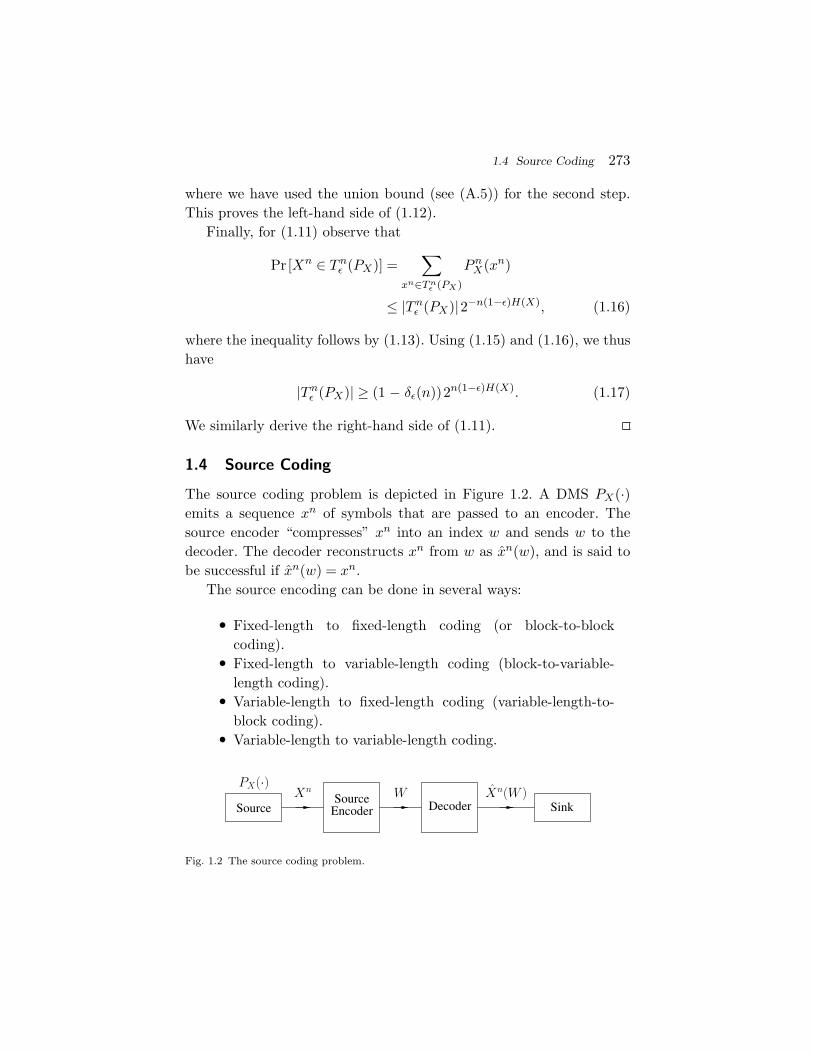


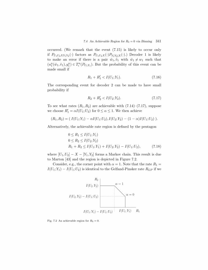


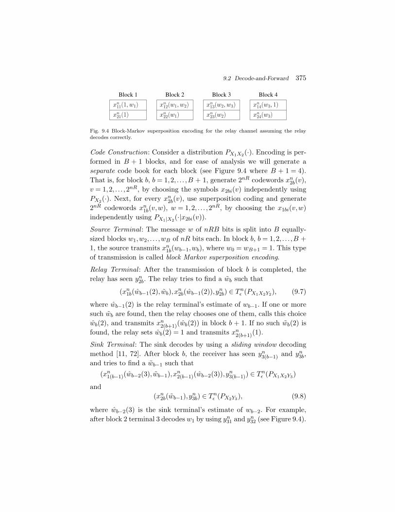


![[XLS] · Web view1 2 2 2 3 2 4 2 5 2 6 2 7 8 2 9 2 10 11 12 2 13 2 14 2 15 2 16 2 17 2 18 2 19 2 20 2 21 2 22 2 23 2 24 2 25 2 26 2 27 28 2 29 2 30 2 31 2 32 2 33 2 34 2 35 2 36 2](https://static.documents.pub/doc/80x56/5ae0cb6a7f8b9a97518daca8/xls-view1-2-2-2-3-2-4-2-5-2-6-2-7-8-2-9-2-10-11-12-2-13-2-14-2-15-2-16-2-17-2.jpg)
![file.henan.gov.cn · : 2020 9 1366 2020 f] 9 e . 1.2 1.3 1.6 2.2 2.3 2.4 2.5 2.6 2.7 2. 2. 2. 2. 2. 2. 2. 2. 2. 2. 2. 2. 2. 2. 2. 2. 2. 2. 2. 2. 17](https://static.documents.pub/doc/80x56/5fcbd85ae02647311f29cd1d/filehenangovcn-2020-9-1366-2020-f-9-e-12-13-16-22-23-24-25-26-27.jpg)


![[XLS] · Web view1 2 2 2 3 2 4 2 5 2 6 2 7 2 8 2 9 2 10 2 11 2 12 2 13 2 14 2 15 2 16 2 17 2 18 2 19 2 20 2 21 2 22 2 23 2 24 2 25 2 26 2 27 2 28 2 29 2 30 2 31 2 32 2 33 2 34 2 35](https://static.documents.pub/doc/80x56/5aa4dcf07f8b9a1d728c67ae/xls-view1-2-2-2-3-2-4-2-5-2-6-2-7-2-8-2-9-2-10-2-11-2-12-2-13-2-14-2-15-2-16-2.jpg)

