Page 1
Kriging and Cross-validation for Massive Spatial Data
Hao Zhang
Department of Statistics
Purdue University
West Lafayette, IN 47907
U.S.A
Phone: (765)496-9548
[email protected]
Yong Wang
Department of Statistics
Purdue University
West Lafayette, IN 47907
U.S.A
[email protected]
Page 2
Kriging and Cross-validation for Massive Spatial Data
February 27, 2009
Abstract
Spatial prediction such as kriging involves the inversion of a covariance matrix. When the number
of locations is very large as in many studies, inversion of the covariance matrix may not be practical.
Covariance tapering, predictive process models and low rank kriging are some methods for overcoming
the large matrix problem, all of which can be regarded as approximations to the underlying stationary
process. Therefore, efficient cross-validation is very helpful for spatial prediction with large data to assess
how well an approximation works. This work studies the calculation of drop-one prediction and various
prediction scores. Estimators are constructed to minimize some prediction scores. One advantage of this
approach is that it integrates estimation and cross-validation and does not treat them as two separate
procedures. Further simplification of calculation is studied that is based on the infill asymptotic theory.
The methods are illustrated through the analysis of a US precipitation dataset.
Keywords: cross-validation; infill asymptotics; low rank kriging; predictive process model; predictive
scores; Woodbury formula;
1 Introduction
Due to the technology advancement, massive data are often observed at a large number of spatial locations
in environmental, ecological and climate studies. These massive data present a challenge to the adoption of
the well-studied inferential methods such as the maximum likelihood estimation, the Bayesian methods and
best linear prediction (kriging) because these methods require the inversion of a large covariance matrix. In
recent years, there have been several approaches to overcoming this large matrix problem. Some take the
computational advantage of sparse matrices as in the covariance tapering (Furrer et al., 2006; Zhang and Du,
2008) and some put a low rank structure on the covariance matrix that enables us to calculate the inverse of
a large covariance by inverting a matrix of lower dimension according to the Woodbury formula (e.g., Cressie
and Johannesson, 2008; Banerjee et al., 2008). Some adopts the spectral method for parameter estimation
(e.g., Fuentes, 2007) although this method does not overcome the difficulty in prediction with massive data.
1
Page 3
The following low rank model has been employed in different forms (e.g., Higdon, 1998; Cressie and
Johannesson, 2008; Stein, 2008; Banerjee et al., 2008)
Y (s) = x(s)′β + a(s)′Z + ε(s), (1)
where x(s) is a vector of covariates, β is a vector of parameters, a(s) = (a1(s), · · · , am(s))′ is a function of
s that may depend on some parameters θ, Z = (Z(u1), · · · , Z(um))′ is a vector of latent variables, and ε(s)
is a white noise with variance τ2 and is independent of Z.
Model (1) includes the Gaussian process convolution (Higdon, 1998) for which aj(s) = exp(−‖s− uj‖2 /φ)/√
2π
is given by the Gaussian kernel where uj ’s are some known spatial locations and φ is the band width
parameter. It also includes the predictive process model in Banerjee et al. (2008) for which a(s) =
V ar(Z)−1Cov(Z, Z(s)) where Z(s) is a Gaussian stationary process with mean 0 and some parametric
covariogram, and the model for fixed rank kriging (Cressie and Johannesson, 2008) for which aj(s) =
b(‖s− uj‖2 /φ) for some known basis function b and Z = (Z(u1), · · · , Z(um)′ is a realization of a latent
process at locations uj , j = 1, · · · ,m.
When the process Y (s) is observed at n locations, say, s1, · · · , sn, the low rank model can be written as
Y = Xβ + AZ + ε.
The covariance matrix of Y is
V = AVzA′ + τ2In,
where In is the n×n identity matrix and Vz = V ar(Z), and A is n×m. Due to the this particular structure,
the inverse of V can be given by inverting only an m×m matrix by the Woodbury formula (Harville, 1997),
V −1 = τ−2(In −A(τ2V −1z + A′A)−1A′). (2)
Therefore, one would be able to compute the kriging predictor for Y (s), which can be expressed as
Y (s) = x(s)′β + a(s)′Z
where the Z = VzA′V −1(Y −Xβ) is the best linear predictor for Z. It follows (2) that we can calculate Z
without inverting the n× n covariance matrix:
Z = (τ2V −1z + A′A)−1A′Y
which involves the inverse of an m×m matrix. The computational simplification results from the fact that
only m variables Z1, · · · , Zm are used in the representation of the process Y (s).
For parameter estimations in the low rank model (1), Bayesian methods are often used with the Markov
chain Monte Carlo techniques (Higdon, 1998; Banerjee et al., 2008). Cressie and Johannesson (2008) used
2
Page 4
moments estimators to for the variance parameters in K and τ2. Stein (2008) discussed a computational
method for calculating the Gaussian likelihood function.
On the other hand, it is often the case that for prediction at a location, observations nearer to the
prediction location have the largest impact on the kriging predictor. This has long been known in geostatistics
literature as the screening effect. Stein (2002) justified the screening effect by the infill or fixed-domain
asymptotic theory. Therefore, one may use only a subset of nearest neighbors to make the prediction. This
is common practice in geostatistics and has implemented in ArcGIS. Haas (1990, 1995) called it the moving
window kriging.
Although the local kriging effectively overcomes the large matrix problem, one difficulty of moving window
kriging is the repeated estimation of parameters within each window or neighborhood. Haas (1990, 1995)
used the least squares method to estimate the variogram within each neighborhood although some numerical
studies have shown that the maximum likelihood estimation usually has superior predictive performance
(Zimmerman and Zimmerman, 1991; Zhang and Zimmerman, 2007). However, repeated estimation by
maximizing the likelihood function greatly increases the computational time. On the other hand, if these
parameters are not re-estimated and the same estimates are used in all neighborhoods as in the ArcGIS
software, the local kriging may not achieve the best predictive performance it could. The other reason for
estimation within each neighborhood is that the underlying process may not be stationary globally but is
more likely to be approximately stationary within a neighborhood. By estimating the parameters within a
neighborhood under the assumption of stationarity, we could arrive at prediction results that are better than
those obtained using all data.
The purpose of this paper is to further simplify the computation for parameter estimation for massive
spatial data without scarifying predictive performance. For this purpose, we first develop an efficient com-
puting algorithm for calculating different predictive scores that are measures of the predictive performance.
We introduce an estimation method that minimizes some predictive scores and apply the method to the lower
rank model and the local kriging. We illustrate this method through a real dataset on the US precipitation.
2 Kriging and predictive scores
Our aim is to develop an efficient algorithm for both parameter estimation and the evaluation of predictive
performance. For now let us assume that the underlying process is stationary with a covariogram C(h) =
σ2ρ(h/φ) where ρ is the correlation function and could depend on an additional parameter.
Empirical studies have shown that in most cases the parameter φ only slightly affects the interpolation
and it is a function of σ2 and φ that primarily affects the interpolation. Theoretical results explain why φ
does not significantly affect the interpolation when the covariogram is in the Matern class. Indeed, for the
3
Page 5
Matern covariogram
C(h) =σ2(h/φ)ν
2ν−1Γ(ν)Kν(h/φ), h ≥ 0, (3)
by employing the infill asymptotic theory (e.g., Stein, 1999), Zhang (2004) showed theoretically and illus-
trated numerically that it is the ratio σ2/φ2ν that matters more to interpolation. Indeed, a misspecified
Matern model with the correct ratio yields an asymptotically optimal interpolator. Furthermore, we can
fix φ at an arbitrary value φ1 and estimate the variance σ2 by maximizing the likelihood function. Zhang
(2004) showed that σ2/φ2ν1 is a consistent estimator of σ2/φ2ν . Recently, Du, Zhang, and Mandrekar (2009)
showed that σ2/φ2ν1 is asymptotically efficient. All these theoretical results imply that we can fix φ and
estimate other parameters and will not suffer any substantial loss of predictive performance. Zhang and
Zimmerman (2007) used exactly this idea and proposed hybrid estimators by fixing φ at the weighted least
squares estimate. Their numerical results show that the hybrid estimators have a predictive performance
that is comparable with that of the exact MLE but superior than that of the least squares method even for
some non-Matern covariograms for which the theoretical results are not yet available.
When the covariogram has a nugget effect τ2, i.e., C(h) = σ2ρ(h/φ) + τ21{h=0} where 1{h=0} is the
indicator function and take the value 1 if h = 0 and 0 otherwise, the similar conclusion still holds, i.e., what
matters more to prediction is the nugget effect τ2 and the ratio σ2/φ2ν for the Matern model. The hybrid
estimator works well in the presence of a nugget effect as shown by the results of Zhang and Zimmerman
(2007).
What is useful though would be an efficient algorithm that evaluates the predictive performance. Predic-
tive performance is usually measured by some predictive scores. Gneiting and Raftery (2007) and Gneiting
et al. (2007) discussed several predictive scores that are reviewed below, all of which are based on the drop-one
prediction.
2.1 Predictive score
Given observations Y (si) made at locations si for i = 1, · · · , n, we denote by Y−i(si) the best linear prediction
based on all data Y (sj) for j 6= i. This is commonly called the drop-one prediction. Let σ2−i be the
corresponding drop-one prediction variance. Write
zi =Y (si)− Y−i(si)
σ−i, i = 1, · · · , n. (4)
One predictive score is the root-mean-square error (RMSE),
RMSE =
{1n
n∑
i=1
(Y (si)− Y−i(si)
)2}1/2
.
4
Page 6
The RMSE is commonly used in cross-validation. Another score that incorporates the prediction variance
is the logarithmic score
LogS =1n
n∑
i=1
(12
log(2πσ−i(si)2) +12z2i
)(5)
where zi is defined in (4).
The following two scores utilize the explicit predictive distribution. The Brier score is defined as (Brier,
1950)
BS(y) =1n
n∑
i=1
(Fi(y)− 1{Y (si) ≤ y})2
. (6)
where Fi(y) is the predictive cdf of Y (si), namely, Fi(y) = P (Y (si) ≤ y|Y (sj), j 6= i), and 1{Y (si) ≤ y} is
the indicator function and takes the value 1 if Y (si) ≤ y and 0 otherwise. When the underlying process is
Gaussian, the predictive distribution for Yi(si) is N(Y−i(si), σ−i(si)2). The continuous ranked probability
score is the integration of BS(y) over the y ∈ (−∞,∞):
CRPS =1n
n∑
i=1
∫ ∞
−∞
(Fi(y)− 1{Y (si) ≤ y})2
dy =∫ ∞
−∞BS(y)dy. (7)
If Y = (Y (s1), · · · , Y (sn))′ has a multivariate normal distribution, CRPS can be calculated based on the
zi’s in (4) (see, Gneiting et al., 2007):
CRPS =1n
n∑
i=1
σ−i(si)(
zi (2Φ(zi)− 1) + 2Φ(zi)− 1√π
)(8)
All these predictive scores require the computation of the drop-one predictions Y−i(si) and prediction vari-
ance σ−i(si)2. We could of course calculate iteratively all these drop-one predictions but this would be
computationally inefficient. Therefore for large spatial data, we should avoid the iterative calculation of
the drop-one prediction. Next we show how they can be calculated efficiently without iteration. Then it is
feasible to minimize a predictive score to obtain parameter estimates for superior predictive performance.
2.2 Calculation of drop-one prediction
Let us temporarily assume that EY (s) = 0 and write Yi = Y (si) for brevity. Write the observed variables
in vector form Y = (Y1, · · · , Yn)′ and assume V ar(Y ) = V . Let qij be the (i, j)th element of V −1. It is well
known that the drop-one prediction for Yi is
Y−i = −∑
j 6=i
qijYj/qii.
Therefore
Yi − Y−i =1qii
n∑
j=1
qijYj (9)
σ2−i = E(Yi − Y−i)2 = 1/qii. (10)
5
Page 7
If we let Λ = diag(qii, i = 1, · · · , n), we have
MSE =1n
n∑
i=1
(Yi − Y−i)2 =1n
∥∥Λ−1V −1Y∥∥2
, (11)
and the zi’s in (4) can be given in vector form
z = Λ−1/2V −1Y .
Let us apply these results to the low rank model (1) for which V is usually a large matrix and its inverse
is computed by the Woodbury formula. We assume that the latent process Z(s) has a constant variance σ2
so that V ar(Z) = σ2Rz. Write w = τ2/σ2, and
Γ = A(wR−1z + A′A)−1A′ = (ARz)
(wRz + (ARz)′(ARz)
)−1(ARz)′. (12)
Then
V −1 = τ−2(In − Γ), and
MSE =1n
∥∥(In − γ)−1(In − Γ)Y∥∥2
(13)
where γ is a diagonal matrix consisting of the diagonal elements of Γ.
When the means are not all zeros, we center the variable by replacing Y by Y −EY . For example, the
MSE given by (13) now becomes
MSE =1n
∥∥(In − γ)−1(In − Γ)(Y − EY )∥∥2
. (14)
In reality, the means have to be estimated. Let us consider the simple case that the mean is a constant
as in the ordinary kriging. In this case, the best linear unbiased estimator of µ is
µ =1′V −1Y
1′V −11.
Then the drop-one prediction error is now
Yi − Y−i = (1/qii)n∑
j=1
qij(Yj − µ).
However, when the mean is estimated, it is no longer true that E(Yi − Y−i)2 = 1/qii. Indeed, if we let
qi = (qij , j = 1, · · · , n)′, we can write
Yi − Y−i =1qii
q′i
(In − 11′V −1
1′V −11
)Y . (15)
Simple calculation yields that
σ2−i = E(Yi − Y−i)2 =
1q2ii
(qii − (q′i1)2
1′V −11
). (16)
6
Page 8
The standardized prediction error in (4) now equals
zi =(
qii − (q′i1)2
1′V −11
)−1/2
q′i
(In − 11′V −1
1′V −11
)Y . (17)
We note that kriging is often carried out in terms of the semivariogram. Dubrule (1983) presented an
algorithm for calculating the drop-one predictions using the semivariogram, which avoids repeated calculation
of (n− 1)× (n− 1) matrices. However, for the low rank model (1), it is more convenient to use covariogram
than semivariogram.
3 Estimation to optimize predictive scores
In this section, we develop an algorithm for estimation that minimizes some predictive scores. We will
estimate the mean parameters by the best linear unbiased estimators, which is identical to the MLE if the
joint distribution is normal, and estimate the parameters in the correlation function by minimizing the MSE,
and variance by minimizing the logarithmic score. In the next two subsections, we will consider the algorithm
for the predictive process model, which is capable of handing very large datasets, and also the local kriging.
3.1 Predictive process models
We assume that the underlying process Y (s) follows the predictive process model as defined in Banerjee et al.
(2008): Let W (s) be a stationary process with mean 0 and covariogram σ2ρ(h, φ), where φ is a parameter
and could be a vector. Let u1, · · · ,um be the m known locations, also called “knots” by Banerjee et al.
(2008). The predictive process model is
Y (s) = µ + k(s)′R−1W + ε(s), (18)
where W = (W (u1), · · · ,W (um))′, R is the correlation matrix of W whose (i, j)th element is ρ(ui − uj , φ),
and k(s) = Corr(W, W (s)) is the correlation of W and W (s) whose jth element is ρ(s− uj , φ).
If Y = (Y (s1), · · · , Y (sn)′ represents the observations at n locations, we can write
Y = µ1 + AW + ε,
for A = KR−1 and K = (k(s1), · · · ,k(sn))′ is an n×m matrix (whose (i, j)th element is ρ(si −uj , φ). The
Γ matrix defined in (12) is now, because AR = K,
Γ = K(wR + K ′K)−1K ′. (19)
The best linear unbiased estimator for µ is
µ =1′(In − Γ)Y1′(In − Γ)1
. (20)
7
Page 9
Note µ depends on w and φ, which are estimated by minimizing the MSE (14), i.e.,
(w, φ) = ArgMinw,φ
∥∥(In − γ)−1(In − Γ)(Y − µ1)∥∥2
. (21)
We estimate the nugget effect τ2 by minimizing the logarithmic score (5). Let γij denote the (i, j)th element
of Γ and γi = (γij , j = 1, · · · , n)′. Since V −1 = τ−2(In − Γ), from (16),
σ2−i = τ2
(1
1− γii− 1
(1− γii)2(1− γ′i1)2
n− 1′Γ1
)= α2
i τ2. (22)
The logarithmic score (5) equals
12
log(2π) +12n
n∑
i=1
(log(τ2α2
i ) +(Yi − Y−i)2
α2i τ
2
)
Minimizing LogS leads to the estimator
τ2 =1n
n∑
i=1
(Yi − Y−i)2
α2i
. (23)
This is clearly an unbiased estimator for τ2. We note that the vector of α2i , i = 1, · · · can be calculated easily
in R by the following, where G is the Γ matrix:
1/(1-diag(G))-(1-rowSums(G))^2/((1-diag(G))^2*(n-sum(G)))
One may also estimate τ2 by the following estimator, which is obtained by maximizing the likelihood
function when all other parameters are fixed at the their estimates:
τ2mle =
1n
(Y − µ1)′(In − Γ)(Y − µ1). (24)
This estimator is biased and leads to higher LogS score than τ2 in (23). Since our primary objective is
spatial prediction with lower predictive scores, we will use the estimator (23) in this work.
We note that the maximum likelihood estimators for all parameters are attainable for the predictive
process model as will be discussed in the example of next section. However, the likelihood function can be
quite flat at the maximum point which can cause some numerical optimization algorithms to stop working.
Although the predictive scores can be flat too, the flatness tells us that the prediction is not sensitive to the
parameter values and we therefore could use any parameter value in the region where the scores are flat.
This is an advantage of the finding estimates through the predictive scores. These estimates require less
computation than the maximum likelihood estimates because we do not need to evaluate the determinant.
3.2 Local kriging
As in the previous section, we assume the correlation function ρ depends on a parameter φ which could be
a vector. We will get a rough estimate for the parameter and treat the the parameter as being known in
8
Page 10
the local kriging. Such a rough estimate can be obtained by the least squares methods using all data or the
maximum likelihood method using a subset of data. The parameters to be estimated in each neighborhood
are therefore µ, σ2 and τ2. Here we consider the case that in each neighborhood EY (s) = µ is a constant and
the process is stationary. To predict at a location s0, we first find the nearest m locations and let Y 0 denote
the observations at the m locations. Write the covariance of the m observed variables as V = σ2R + τ2. We
estimate w = τ2/(τ2 + σ2) by minimizing the sum of squared errors:
w = ArgMinw
∑
si∈Oi
(Y (si)− Y−i(si))2 = ArgMinw
∥∥D−1(wI + (1 + w)R)−1(Y 0 − µ(w)1)∥∥2
(25)
where Oi is the set of m nearest locations, D is a diagonal matrix consisting of the diagonal elements of
(wI + (1 + w)R)−1, 1 is the vector of all 1’s, and µ = µ(w) is the best linear unbiased estimator of µ, i.e.,
µ(w) =1′(wI + (1 + w)R)−1Y
1′(wI + (1 + w)R)−11.
Once w is obtained, µ is estimated by µ(w) and the sill σ2 + τ2 is estimated by
1m
∑
si∈Oi
γii(Y (si)− Y−i(si))2
where γii is the ith diagonal element of the matrix (wI + (1 + w)R)−1.
4 An example
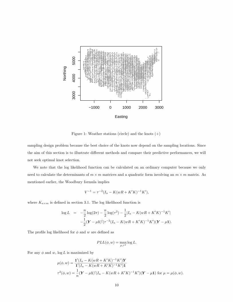
In this section, we illustrate the methods by applying them to a set of US precipitation data which consists
of the monthly total precipitation record in the conterminous US for April 1948 consisting of 5,906 stations.
The standardized square root values, known as anomalies, are analyzed here. The anomaly data are available
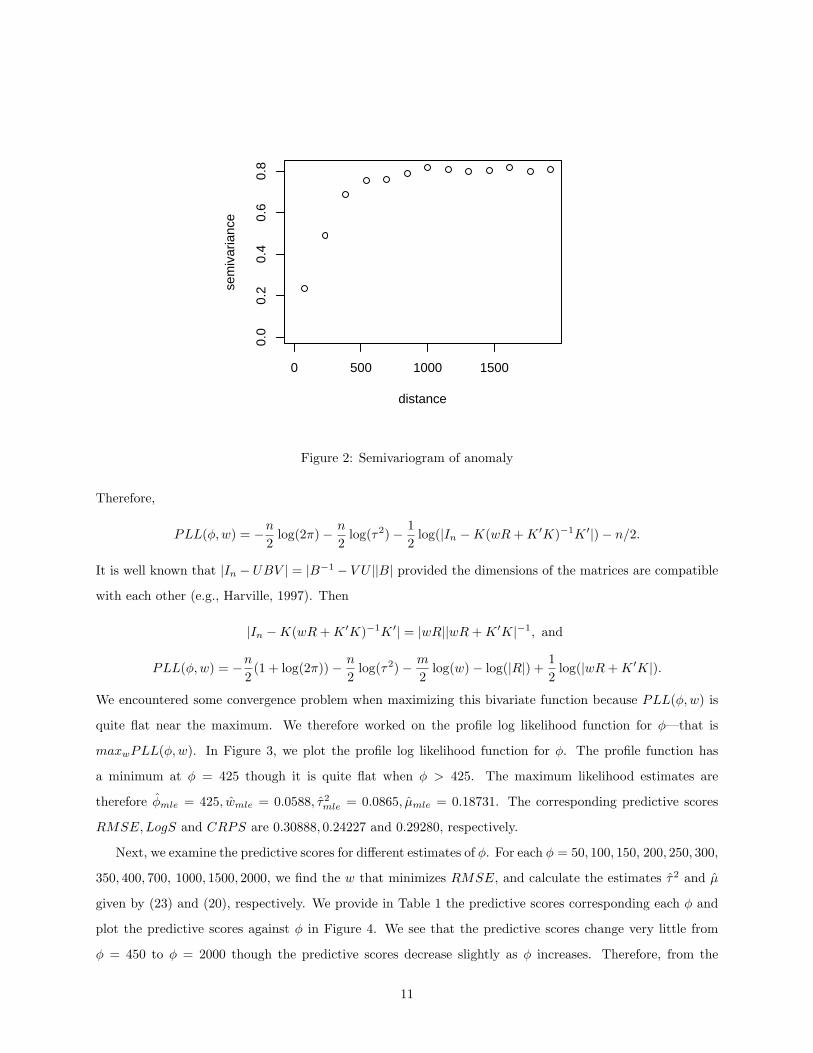
in the R package spam. The weather stations are shown in Figure 1 and the empirical semivariogram is plotted
in Figure 2. We will use an exponential covariogram with a nugget effect and assume a constant mean.
We first employ the predictive process model with m = 760 knots. The knots are marked in Figure 1
by “+”. The number of knots is usually kept to be below 1,000 as in Cressie and Johannesson (2008) and
Banerjee et al. (2008). The number of knots we use here is larger than theirs (396 in Cressie and Johannesson
and 144 in Banerjee et al.) though the sample size in this example is smaller than theirs (173,405 and 9,500 in
Cressie and Johannesson and Banerjee et al., respectively). The evenly spaced knots are desirable in practice
from the prediction point of view though it may not be the optimal design. Although it is possible in principle
to find the best design, one may double about the worth of possible gains in prediction precision relative to
the computational effort. Furthermore, Banerjee et al. (2008) compared knots on a regular lattice with knots
on a regular knots plus some infill knots which are closer together and found little difference between the
prediction results given by the two sets of knots. Finally, we note that the choice of knots is not the classical
9
Page 11
−1000 0 1000 2000 3000
3000
4000
5000
Easting
Nor
thin
g
+ + ++ + + +
+ + + + + ++ + + + +
+ + + + + + + + + + + + ++ + + + + + + + + + + + + +
+ + + + + + + + + + + + + + + + + ++ + + + + + + + + + + + + + + + + + + +
+ + + + + + + + + + + + + + + + + + + + + ++ + + + + + + + + + + + + + + + + + + + + +
+ + + + + + + + + + + + + + + + + + + + + + + + + ++ + + + + + + + + + + + + + + + + + + + + + + + + + +
+ + + + + + + + + + + + + + + + + + + + + + + + + + + ++ + + + + + + + + + + + + + + + + + + + + + + + + + + + +
+ + + + + + + + + + + + + + + + + + + + + + + + + + + + + + ++ + + + + + + + + + + + + + + + + + + + + + + + + + + + + + ++ + + + + + + + + + + + + + + + + + + + + + + + + + + + + + ++ + + + + + + + + + + + + + + + + + + + + + + + + + + + + + ++ + + + + + + + + + + + + + + + + + + + + + + + + + + + + + +
+ + + + + + + + + + + + + + + + + + + + + + + + + + + + + + + ++ + + + + + + + + + + + + + + + + + + + + + + + + + + + + + + ++ + + + + + + + + + + + + + + + + + + + + + + + + + + + + + + ++ + + + + + + + + + + + + + + + + + + + + + + + + + + + + + + ++ + + + + + + + + + + + + + + + + + + + + + + + + + + + + + + ++ + + + + + + + + + + + + + + + + + + + + + + + + + + + + + + +
+ + + + + + + + + + + + + + + + + + + + + + + + + + + + + + ++ + + + + + + + + + + + + + + + + + + + + + + + + + + + ++ + + + + + + + + + + + + + + + + + + + + + + + + + + + ++ + + + + + + + + + + + + + + + + + + + + + + + + + + +
+ + + + + + + + + + + + + + + + + + + + + + ++ + + + + + + + + + + + + + + + ++ + + + + + + + + ++ + + + + + +
+ +
Figure 1: Weather stations (circle) and the knots (+)
sampling design problem because the best choice of the knots now depend on the sampling locations. Since
the aim of this section is to illustrate different methods and compare their predictive performances, we will
not seek optimal knot selection.
We note that the log likelihood function can be calculated on an ordinary computer because we only
need to calculate the determinants of m×m matrices and a quadratic form involving an m×m matrix. As
mentioned earlier, the Woodbury formula implies
V −1 = τ−2(In −K(wR + K ′K)−1K ′),
where Kn×m is defined in section 3.1. The log likelihood function is
log L = −n
2log(2π)− n
2log(τ2)− 1
2|In −K(wR + K ′K)−1K ′|
−12(Y − µ1)′(τ−2(In −K(wR + K ′K)−1K ′)(Y − µ1).
The profile log likelihood for φ and w are defined as
PLL(φ,w) = maxµ,τ2
log L.
For any φ and w, log L is maximized by
µ(φ,w) =1′(In −K(wR + K ′K)−1K ′)Y1′(In −K(wR + K ′K)−1K ′)1
τ2(φ,w) =1n
(Y − µ1)′(In −K(wR + K ′K)−1K ′)(Y − µ1) for µ = µ(φ,w).
10
Page 12
0 500 1000 1500
0.0
0.2
0.4
0.6
0.8
distance
sem
ivar
ianc
e
Figure 2: Semivariogram of anomaly
Therefore,
PLL(φ,w) = −n
2log(2π)− n
2log(τ2)− 1
2log(|In −K(wR + K ′K)−1K ′|)− n/2.
It is well known that |In −UBV | = |B−1 − V U ||B| provided the dimensions of the matrices are compatible
with each other (e.g., Harville, 1997). Then
|In −K(wR + K ′K)−1K ′| = |wR||wR + K ′K|−1, and
PLL(φ,w) = −n
2(1 + log(2π))− n
2log(τ2)− m
2log(w)− log(|R|) +
12
log(|wR + K ′K|).
We encountered some convergence problem when maximizing this bivariate function because PLL(φ,w) is
quite flat near the maximum. We therefore worked on the profile log likelihood function for φ—that is
maxwPLL(φ,w). In Figure 3, we plot the profile log likelihood function for φ. The profile function has
a minimum at φ = 425 though it is quite flat when φ > 425. The maximum likelihood estimates are
therefore φmle = 425, wmle = 0.0588, τ2mle = 0.0865, µmle = 0.18731. The corresponding predictive scores
RMSE,LogS and CRPS are 0.30888, 0.24227 and 0.29280, respectively.
Next, we examine the predictive scores for different estimates of φ. For each φ = 50, 100, 150, 200, 250, 300,
350, 400, 700, 1000, 1500, 2000, we find the w that minimizes RMSE, and calculate the estimates τ2 and µ
given by (23) and (20), respectively. We provide in Table 1 the predictive scores corresponding each φ and
plot the predictive scores against φ in Figure 4. We see that the predictive scores change very little from
φ = 450 to φ = 2000 though the predictive scores decrease slightly as φ increases. Therefore, from the
11
Page 13
200 400 600 800 1000
300
500
700
phi
prof
ile lo
g lik
elih
ood
Figure 3: The profile log likelihood for φ.
0 500 1000 1500 2000
0.24
0.26
0.28
0.30
0.32
0.34
phi
RM
SE
Figure 4: Predictive scores against φ: RMSE (solid line), LogS (dotted line) and CRPS (dashed line)
12
Page 14
φ w τ2 RMSE LogS CRPS p
1 50 0.16179 0.10209 0.33803 0.33621 0.31834 0.05689
2 100 0.15442 0.08791 0.31323 0.26115 0.29672 0.05621
3 150 0.11937 0.08637 0.31057 0.25226 0.29498 0.05571
4 200 0.09427 0.08584 0.30968 0.24926 0.29444 0.05604
5 250 0.07723 0.08559 0.30926 0.24784 0.29418 0.05621
6 300 0.06521 0.08546 0.30902 0.24705 0.29402 0.05604
7 350 0.05634 0.08537 0.30888 0.24657 0.29391 0.05588
8 400 0.04954 0.08531 0.30878 0.24624 0.29384 0.05588
9 700 0.02863 0.08519 0.30856 0.24552 0.29366 0.05604
10 1000 0.02010 0.08515 0.30851 0.24533 0.29361 0.05604
11 1500 0.01343 0.08514 0.30848 0.24523 0.29358 0.05604
12 2000 0.01005 0.08513 0.30847 0.24520 0.29357 0.05604
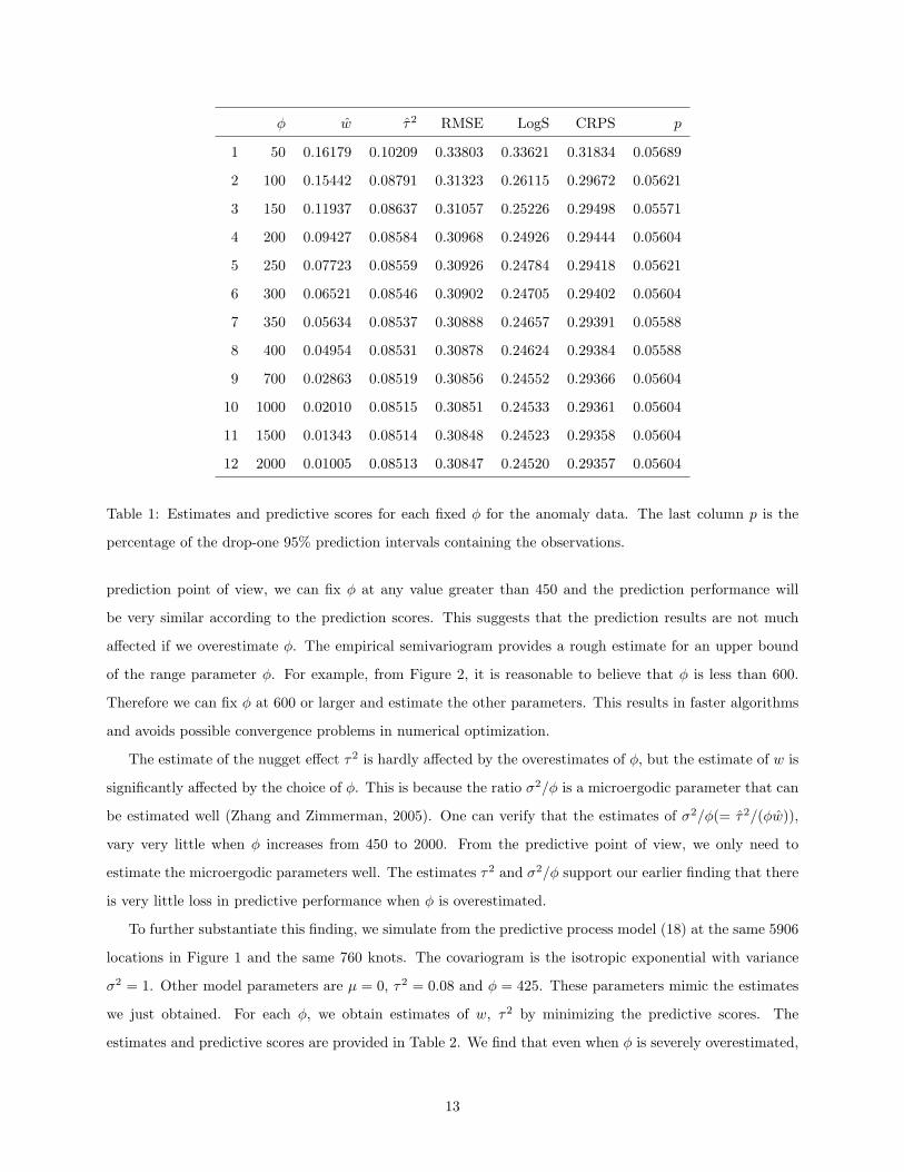
Table 1: Estimates and predictive scores for each fixed φ for the anomaly data. The last column p is the
percentage of the drop-one 95% prediction intervals containing the observations.
prediction point of view, we can fix φ at any value greater than 450 and the prediction performance will
be very similar according to the prediction scores. This suggests that the prediction results are not much
affected if we overestimate φ. The empirical semivariogram provides a rough estimate for an upper bound
of the range parameter φ. For example, from Figure 2, it is reasonable to believe that φ is less than 600.
Therefore we can fix φ at 600 or larger and estimate the other parameters. This results in faster algorithms
and avoids possible convergence problems in numerical optimization.
The estimate of the nugget effect τ2 is hardly affected by the overestimates of φ, but the estimate of w is
significantly affected by the choice of φ. This is because the ratio σ2/φ is a microergodic parameter that can
be estimated well (Zhang and Zimmerman, 2005). One can verify that the estimates of σ2/φ(= τ2/(φw)),
vary very little when φ increases from 450 to 2000. From the predictive point of view, we only need to
estimate the microergodic parameters well. The estimates τ2 and σ2/φ support our earlier finding that there
is very little loss in predictive performance when φ is overestimated.
To further substantiate this finding, we simulate from the predictive process model (18) at the same 5906
locations in Figure 1 and the same 760 knots. The covariogram is the isotropic exponential with variance
σ2 = 1. Other model parameters are µ = 0, τ2 = 0.08 and φ = 425. These parameters mimic the estimates
we just obtained. For each φ, we obtain estimates of w, τ2 by minimizing the predictive scores. The
estimates and predictive scores are provided in Table 2. We find that even when φ is severely overestimated,
13
Page 15
φ w τ2 RMSE LogS CRPS p
1 50 0.09842 0.09535 0.32664 0.30679 0.32810 0.04724
2 100 0.21213 0.07878 0.29650 0.20316 0.29833 0.05012
3 150 0.19031 0.07805 0.29467 0.19709 0.29597 0.04961
4 200 0.15745 0.07796 0.29432 0.19607 0.29529 0.04961
5 250 0.13159 0.07794 0.29422 0.19581 0.29503 0.05029
6 300 0.11230 0.07794 0.29419 0.19575 0.29491 0.05012
7 350 0.09762 0.07794 0.29418 0.19574 0.29486 0.05046
8 400 0.08619 0.07795 0.29418 0.19575 0.29483 0.05046
9 700 0.05027 0.07797 0.29421 0.19583 0.29480 0.05029
10 1000 0.03542 0.07798 0.29422 0.19588 0.29481 0.05029
11 1500 0.02366 0.07799 0.29423 0.19592 0.29483 0.05029
12 2000 0.01775 0.07799 0.29423 0.19594 0.29484 0.05029
Table 2: Estimates and predictive scores for each fixed φ for the simulated data with the exponential
covariogram. The last column p is the percentage of the drop-one 95% prediction intervals containing the
observations.
the predictive scores are very little affected.
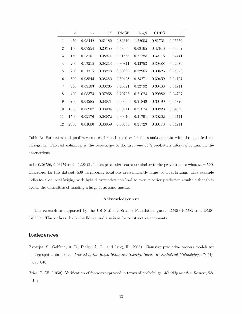
Next, we simulate the predictive process model (18) with a spherical covariogram having a range φ = 425.
The sampling locations and knots are the same and the model parameters are σ2 = 1, µ = 0, and τ2 = 0.08.
The estimates and predictive scores are provided in Table 3. Similar conclusions hold although there is no
infill asymptotic theoretical results established for the spherical covariogram.
We now revisit the anomaly data and apply local kriging with the exponential covariogram with a nugget
effect. The range parameter φ is fixed at 425 in every neighborhood and the size of neighborhood is fixed
at m = 500. Within each neighborhood, we minimize the RMSE and the LogS score to estimate the nugget
effect and the partial sill. These estimates vary from neighborhood to neighborhood and will not be reported.
Instead, we will report the predictive scores where the drop-one prediction . At an observed location, say
si, the drop-one prediction Y (si) is calculated using only the nearest m locations. The RMSE, LogS and
CRPS are 0.26702, 0.06453 and −1.40194, respectively. These predictive scores are lower than those in the
predictive process model, which means that this local kriging resulted in better prediction results. This
could be due to the fact that the predictive process model is an approximation to the underlying process or
due to non-stationarity.
We increase the number of neighborhood from m = 500 to m = 800 and obtain RMSE, LogS and CRPS
14
Page 16
φ w τ2 RMSE LogS CRPS p
1 50 0.08442 0.61182 0.83819 1.22903 0.81731 0.05350
2 100 0.07254 0.20355 0.48603 0.69165 0.47616 0.05367
3 150 0.13101 0.08971 0.31863 0.27788 0.32116 0.04741
4 200 0.17215 0.08213 0.30311 0.22753 0.30488 0.04639
5 250 0.11315 0.08248 0.30383 0.22965 0.30626 0.04673
6 300 0.08545 0.08286 0.30458 0.23271 0.30659 0.04707
7 350 0.09103 0.08235 0.30321 0.22792 0.30488 0.04741
8 400 0.08373 0.07958 0.29795 0.21024 0.29982 0.04707
9 700 0.04285 0.08071 0.30033 0.21849 0.30199 0.04826
10 1000 0.03207 0.08084 0.30041 0.21874 0.30223 0.04826
11 1500 0.02176 0.08072 0.30019 0.21791 0.30202 0.04741
12 2000 0.01600 0.08059 0.30003 0.21729 0.30173 0.04741
Table 3: Estimates and predictive scores for each fixed φ for the simulated data with the spherical co-
variogram. The last column p is the percentage of the drop-one 95% prediction intervals containing the
observations.
to be 0.26736, 0.06479 and −1.38466. These predictive scores are similar to the previous ones when m = 500.
Therefore, for this dataset, 500 neighboring locations are sufficiently large for local kriging. This example
indicates that local kriging with hybrid estimation can lead to even superior prediction results although it
avoids the difficulties of handing a large covariance matrix.
Acknowledgement
The research is supported by the US National Science Foundation grants DMS-0405782 and DMS-
0706835. The authors thank the Editor and a referee for constructive comments.
References
Banerjee, S., Gelfand, A. E., Finley, A. O., and Sang, H. (2008). Gaussian predictive process models for
large spatial data sets. Journal of the Royal Statistical Society, Series B: Statistical Methodology , 70(4),
825–848.
Brier, G. W. (1950). Verification of forcasts expressed in terms of probability. Monthly weather Review , 78,
1–3.
15
Page 17
Cressie, N. and Johannesson, G. (2008). Fixed rank kriging for very large data sets. Journal of the Royal
Statistical Society, B , 70, 209–226.
Du, J., Zhang, H., and Mandrekar, V. (2009). Fixed-domain asymptotic properties of tapered maximum
likelihood estimators. Annals of Statistics (In Print).
Dubrule, O. (1983). Cross validation of Kriging in a unique neighborhood. Mathematical Geology , 15(6),
687–699.
Fuentes, M. (2007). Appropriate likelihood for large irregularly spaced spatial data. Journal of the American
Statistical Association, 102, 321–331.
Furrer, R., Genton, M. G., and Nychka, D. (2006). Covariance tapering for interpolation of large spatial
datasets. Journal of Computational and Graphical Statistics, 15(3), 502–523.
Gneiting, T. and Raftery, A. E. (2007). Strictly Proper Scoring Rules, Prediction, and Estimation. Journal
of the American Statistical Association, 102(477), 359–378.
Gneiting, T., Balabdaoui, F., and Raftery, A. E. (2007). Probabilistic forecasts, calibration and sharpness.
Journal of the Royal Statistical Society, Series B: Statistical Methodology , 69(2), 243–268.
Haas, T. C. (1990). Lognormal and moving window methods of estimating acid deposition. Journal of the
American Statistical Association, 85, 950–963.
Haas, T. C. (1995). Local prediction of a spatio-temporal process with an application to wet sulfate deposi-
tion. Journal of the American Statistical Association, 90, 1189–1199.
Harville, D. A. (1997). Matrix Algebra from a Statistician’s Perspective. Springer-Verlag Inc.
Higdon, D. (1998). A process-convolution approach to modelling temperatures in the North Atlantic Ocean
(Disc: P191-192). Environmental and Ecological Statistics, 5, 173–190.
Stein, M. L. (1999). Interpolation of Spatial Data: Some Theory for Kriging . Springer, New York.
Stein, M. L. (2002). The screening effect in kriging. The Annals of Statistics, 30(1), 298–323.
Stein, M. L. (2008). A modeling approach for large spatial datasets. Journal of the Korean Statistical Society ,
37, 3–10.
Zhang, H. (2004). Inconsistent estimation and asymptotically equivalent interpolations in model-based
geostatistics. Journal of the American Statistical Association, 99, 250–261.
16
Page 18
Zhang, H. and Du, J. (2008). Covariance tapering in spatial statistics. In J. Mateu and E. Porcu, editors,
Positive definite functions: From Schoenberg to space-time challenges, pages 181–196.
Zhang, H. and Zimmerman, D. L. (2005). Towards reconciling two asymptotic frameworks in spatial statistics.
Biometrika, 92, 921–936.
Zhang, H. and Zimmerman, D. L. (2007). Hybrid estimation of semivariogram parameters. Mathematical
Geology , 39, 247–260.
Zimmerman, D. L. and Zimmerman, M. B. (1991). A comparison of spatial semivariogram estimators and
corresponding ordinary kriging predictors. Technometrics, 23, 77–91.
17