Kriging-Based Probabilistic Method for Constrained Multi-Objective Optimization Problem

Shinkyu Jeong* Tohoku University, Sendai, Miyagi, 980-8577, Japan

Kazuomi Yamamoto†

Japan Aerospace Exploration Agency, Chofu, Tokyo, 182-8522, Japan

and

Shigeru Obayashi‡

Tohoku University, Sendai, Miyagi, 980-8577, Japan

In this paper, Kriging model is applied to a constrained multi-objective optimization problem. In order to balance the local and global search in the Kriging model, the criterion ‘expected improvement (EI)’ is adopted. Probability of satisfying the constraints is calculated in the Kriging model to impose the constraint effect into EI. Search region of the design space is modified during the optimization by investigating the distribution of the design variables. Functional analysis of variance (ANOVA) is performed to identify which design variables are important for the objective and constraint functions. The present method is applied to a transonic airfoil design for the validation.

Nomenclature A = cross-sectional area of airfoil

),( ⋅⋅d = distance function between two points )]([ ⋅IE = expected improvement

DL / = lift to drag ratio r′ = vector of correlation values for Kriging model R = correlation matrix for Kriging model

)(2 ⋅s = mean squared error of the predictor

)(2 ⋅−is = cross-validated mean squared error of the predictor x = vector denoting position in the design space x = scalar component of x y = vector of response data

)(⋅y = unknown function )(ˆ ⋅y = estimated value of )(⋅y

)(ˆ ⋅−iy = cross-validated prediction

)(⋅Z = deviation from constant model β = constant global model of Kriging model

* Research Associate, Institute of Fluid Science and Associate Member † Team Leader, Information Technology Center and Member AIAA ‡ Professor, Institute of Fluid Science and Associate Fellow

American Institute of Aeronautics and Astronautics

1

β = estimated value of β φ = standard normal density Φ = standard normal distribution η = mean of distribution in normalized search region

totalµ = total mean of model

θ = vector of correlation parameters for Kriging model σ = standard deviation of distribution in normalized search region

2σ = estimated sample variance 2ˆ totalσ = total variance of model

I. Introduction ecently, optimization methods using approximation models1 attract a large attention in the field of aircraft design because it saves a lot computational time for evaluation of objective function. However, it is apt to miss

the true optimum in the design space if the exploration relies only on the estimated function values of the approximation model because these values include uncertainty at unknown points. For the robust exploration of the true optimum with the approximation model, both the estimated function value and its error should be considered at the same time.

R

The Kriging model2-3, developed in the field of spatial statistics and geostatistics, has gained the popularity today. The Kriging model predicts the distribution of function values at an unknown point instead of the function values it self. From the distribution of function values, the function value and its uncertainty at unknown points can be estimated. By using these values, the balanced local and global search is possible. This concept is expressed using the criterion ‘expected improvement (EI)’4. EI indicates the probability of a point being the true optimum in the design space. By selecting maximum EI point as an additional sample point of the Kriging model, the improvement of accuracy and the robust exploration of the true optimum can be achieved at the same time.

In this study, the Kriging model is applied to the constrained multi-objective optimization problem for a transonic airfoil design. The model is constructed for each constraint and objective function. In the Kriging model for the objective function, the expected improvement is calculated. In the Kriging model for the constraint, the probability of satisfying the constraint is calculated. Based on these values, an additional sample point for the balanced local and global search is selected.

Another advantage of using the approximation method is that it shows the relation between the objective function and the design variables. By applying the functional analysis of variance5 (ANOVA) to the approximation model, one can identify which design variables are important for the objective and the constraint functions quantitatively. By using the result of the ANOVA, the present author successfully reduced design variables that have little effect to objective function6.

However, the quantitative result of ANOVA largely depends on regional selection of the design space. If the search region of the design space is changed, this quantitative information is also changed. It means that the design variable which is considered to be negligible may become important in a different region of the design space. Thus, in order to use the ANOVA results effectively, the search region of the design space must be determined adequately. Determination of the search region is very important for the optimization design problem itself. No matter how good an optimizer the designer has, he cannot find a good design solution in an inadequate search region of the design space. Thus, the validity of the search region should be examined and if it is inadequate, the search region should be changed. In this study, the search region of the design space is changed during the optimization process through the validity examination of the search region.

II. Kriging Model The present Kriging model expresses the unknown function y(x) as

)()( xx Zy += µ (1) where is an m-dimensional vector (m design variables), x µ is a constant global model and represents a local deviation from the global model. In the model, the local deviation at an unknown point (x) is expressed using

)(xZ

American Institute of Aeronautics and Astronautics

2

stochastic processes. The sample points are interpolated with the Gaussian random function as the correlation function to estimate the trend of the stochastic processes. The correlation between and is strongly related to the distance between the two corresponding points, x

)( iZ x )( jZ xi and xj. However, the Euclidean distance is not used,

because it weighs all design variables equally. In the Kriging model, a special weighted distance is used instead. The distance function between the point at xi and xj is expressed as

2

1)( j

kik

m

kk

ji xxd −= ∑=θx,x (2)

where kθ )0( ∞≤≤ kθ is the kth element of the correlation vector parameter θ . By using the specially weighted istance and the Gaussian random function, the correlation between the point xi and xj is defined as d

( )[ ] [ ]),(exp),( jiji dZZCorr xxxx −= (3) The Kriging predictor is

)ˆ(ˆ)(ˆ 1 µµ 1yRrx −′+= −y (4)

where µ is the estimated value of µ , R denotes the nn× matrix whose (i, j) entry is [ ])(),( ji ZZCorr xx . r is

vector whose ith element is [ ])(),()( i

i ZZCorrr xxx ≡ (5) and . )](,),........([ 1 nxyxy=y

The detailed derivation of Eq. (4) can be found in [7]. The unknown parameter to be estimated for constructing the Kriging model is θ . This parameter can be estimated by maximizing the following likelihood function

( )

( ) ( )µµσ

σπσµ

ˆˆˆ21

ln21)ˆln(

2)2ln(

2),ˆ,ˆ(

12

22

1yR1y

Rθ

−′−−

−−−=

−

nnLn (6)

where 1 denotes an m-dimensional unit vector. Maximizing the likelihood function is an m-dimensional unconstrained non-linear optimization problem. In this paper, an alternative method8 is adopted to solve this problem.

For a given θ , µ and can be defined as 2σ

1R1yR1

1

1

−

−

′′

=µ (7)

( ) ( )n

µ µσ 1yR1y −′−=

−12ˆ (8)

The accuracy of the prediction value largely depends on the distance from sample points. Intuitively speaking, the closer point x to sample points, the more accurate is the prediction ( )xy . This intuition is expressed in following Equation.

⎥⎦

⎤⎢⎣

⎡′

−+′−=

−

−−

1R1r1RrRrx 1

11

222 )1(1ˆ)( σs (9)

s2(x) is the mean squared error of the predictor. s2(x) indicates the uncertainty at the estimation point. The root mean

squared error (RSME) is expressed as )(2 xss = .

American Institute of Aeronautics and Astronautics

3

III. Expected Improvement and Treatment of Constraint

A. Expected Improvement In order to find the global optimum in the Kriging model, both the estimated function value and the uncertainty

at the unknown point are considered at the same time. Based on these values, the point having the largest probability of being the global optimum is found. The probability of being the global optimum is expressed by the criterion ‘expected improvement (EI)’. The EI in minimization problem is expressed as follows:

(10) ∫ ∞−−=

nfdzzzfsIE min )()()( min φ

where s

yyf n ˆminmin

−= ,

syyzˆ−

= and

[ ]⎩⎨⎧ <−

=otherwise if

0

)()()( minmin yyyy

Ixx

x (11)

B. Treatment of Constraint In order to impose the constraint effect into the optimization problem, the probability of satisfying the constraint

is calculated in the Kriging model. If there are constraints as follows, kiac ii ,.......,1)( => x (12) probabilities of satisfying the constraints9 can be calculated as follow:

)(2

1))((

2)(21

xxx

ia

sac

iii dce

sacP

i

i

ii

∫∞ ⎟⎟

⎠

⎞⎜⎜⎝

⎛ −−

=≥π

))(ˆ(1

i

ii

sac −

Φ−=x (13) ki ,.....,1=

By multiplying these probabilities to conventional EI value, the constraint effects imposed EcI can be calculated as follow: (14) ))(())(())(()()( 11 kkiic acPacPacPIEIE >⋅⋅⋅⋅>⋅⋅⋅⋅>⋅= xxxBased on this value, an additional sample point for the balanced local and global search is selected, while satisfying the constraints.

IV. Functional Analysis of Variance In order to identify the effect of each design variable to the constraints and the objective functions, the total

variance of the model is decomposed into the variance component due to each design variable. It is called the functional analysis of variance (ANOVA). The decomposition is accomplished by integrating variables out of the model . yThe total mean )ˆ( totalµ and variance of model are as follows: ( 2ˆ totalσ ) y (15) ∫ ∫ ⋅⋅⋅⋅⋅⋅⋅⋅≡ nntotal dxdxxxy 11 ),......,(ˆµ

[ ]∫ ∫ ⋅⋅⋅⋅−⋅⋅⋅⋅= nntotal dxdxxxy 12

12 ˆ),......,(ˆˆ µσ (16)

The main effect of variable xi is (17) ∫ ∫ −⋅⋅⋅⋅⋅⋅⋅⋅⋅⋅≡ +− µµ ˆ),,(ˆ)(ˆ 1111 niinii dxdxdxdxxxyx

The two-way interaction of variance xi and xj is µµµµ ˆ)(ˆ)(ˆ ),......,(ˆ),(ˆ 111111, −−−⋅⋅⋅⋅⋅⋅⋅⋅⋅⋅≡ ∫ ∫ +−+− jjiinjjiinjiji xxdxdxdxdxdxdxxxyxx (18)

The variance due to the design variable xi is

( )[ ] iii dxx2

ˆ∫ µ (19)

The proportion of the variance due to design variable xi to total variance of model can be expressed by dividing Eq. (19) with Eq. (16).

American Institute of Aeronautics and Astronautics

4

( )[ ]

[ ]∫ ∫∫

⋅⋅⋅⋅−⋅⋅⋅⋅ nn

iii

dxdxxxy

dxx

12

1

2

ˆ),......,(ˆ

ˆ

µ

µ (20)

This value indicates the sensitivity of the model to the variation of each design variable.

V. Change of Search Region

A. Generation of Superior Population In order to examine the validity of the search region, the superior population (SP) is generated. The meaning of

‘SP’ in this paper is that its individual satisfies all design constraints and the objective function values of its individual are larger than certain values. The simplest way to generate the SP is the Monte-Carlo simulation (MCS). However, MCS requires a large number of function evaluations to generate a moderate number of individuals if superior individuals are distributed in the very small portion of the search region. In this study, the genetic algorithms10 (GAs) is used for the generation of the SP. The GAs used for this purpose requires not to find the global optimum but to maintain diverse individuals whose objective function value is better than a certain value. For this purpose, this method takes advantages of the mutation operation to prevent the convergence of individuals.

B. Distribution Investigation and Search Region Expansion For the generated SP, the distribution of design variables is investigated. Figure 1 shows three types of design

variable distributions.

(a) (b) (c)

Figure 1. Typical types of distributions

In Fig. 1(a), a peak of distribution is located at the middle part of the normalized search region and the density of the design variable is very small near the boundary region. In this case, the probability of superior individuals existing outside of the search region is considered to be very small. Thus, it can be said that the search region for this design variable is relatively reasonable. On the other hand, in Figs. 1(b) and 1(c), the distributions of design variables are concentrated near the boundary region. In these cases, probability of superior individuals existing outside of the search region is considered to be very large. Thus, the search region should be expanded and the region outside of the boundary should be examined whether it has a superior individual or not. The criterion used for the validity check of the search region in this study is as follows:

if(η< 0.05 or η>0.95)then search region is invalid

else if (η-1.96σ<0 .or. η+1.96σ>1)then

search region is invalidelse

search region is validendif

endif

American Institute of Aeronautics and Astronautics

5

If the search region is invalid, the search region is redefined by using following equations.

otherwise σw.ηxσw.., η0.950.05 if σ) .η(xσ.., η(

)961,1max()9610min(961,1max)9610min

21 ⋅+<<⋅−<<+<<− η

(21)

w1 and w2 are weighting parameters which accelerate the convergence of the search region. After the final search region is defined, the converged search region can be defined by using following equation.

σ.ηxσ.η 961961 +<<− (22)

VI. Optimization Problem The present method is applied to a transonic airfoil design. The objective of design is as follows:

Minimize dCsubject to a) 2822_ RAEll CC ≥

b) 2822RAEAreaArea ≅at the flow condition of Mach=0.73 and an angle of attack (AOA) =2.7˚. Cl and Cd are drag and lift coefficient of designed airfoil and Cl_RAE2822 and Cd_RAE2822 are those of RAE2822 airfoil. Area is the cross-sectional area of the airfoil.

A. Definition of Airfoil Geometry and Design Variables The geometry was parameterized by the PARSEC airfoil11. This parameterization technique was developed to

keep the number of design variable as low as possible while controlling important transonic aerodynamic features effectively. Figure 2 illustrates 11 basic parameters for PARSEC airfoil

Parameters are leading edge radius (rLE), upper and lower surface crest location (XUP, ZUP, XLO, ZLO) including the curvature there (ZXXUP, ZXXLO), coordinate (ZTE), thickness (∆ZTE), direction (αTE), and wedge angle ((βTE) of the trailing edge. In this study, only a sharp trailing-edge airfoil was considered, therefore, ∆ZTE was set to zero. A total of 10 design variables were used to define the geometry of airfoil.

B. Initial Search Region The upper and lower bound of each parameter was de

fish-tailed airfoil. The parameter ranges of the search region

Table 1. Parameter r

rLE ZTE αTE βTE XUP

Lower bound 0.007 -0.02 -8° 4° 0.35

Upper bound 0.06 0.02 -3° 8° 0.50

C. Construction of Kriging Model Construction of Kriging model requires 4 steps as show

the search region. It is ideal for the sample points to be scascatter points uniformly in the space is called ‘space-filling’the orthogonal array12 and the Latin hypercube method13, ethe space-filling. This method ensures that a point alwayssample points. A total of 50 sample points (airfoils) are

American Institute of Aero

6

Figure 2. PARSEC airfoil and its parameters

termined to avoid unrealistic airfoil geometry such as a are shown in Table 1.

ange of search region

ZUP ZXXUP XLO ZLO ZXXLO

0.07 -1.0 0.35 -0.12 0.3

0.15 0.2 0.50 -0.07 1.0

in Fig. 3. First, sample points should be selected from ttered uniformly in the search space. The method used to . There are a few kinds of space-filling methods, such as tc. In this study, the Latin hypercube method is used for exists inside the interval partitioned by the number of selected from the initial search region. Second step is

nautics and Astronautics

evaluations at the sample points. The lift and drag performances of 50 sample airfoils were evaluated using a Navier-Stokes code. This code utilized a TVD upwind scheme for spatial discretization of convective terms and a LU-SGS method14 for time integration. With the sample data obtained from the Navier-Stokes analysis, the Kriging parameter (θ) is determined by solving maximization problem of Eq. (6). Once the model is constructed, the model should be validated. The validation is performed by the cross validation5. If the model is valid, all cross-validated values should lie inside of the confidence region. It can be check by using the “standardized cross-validated residual” as follows:

)()(ˆ)(

ii

iii

xsxyxy

−

−− (23)

Figure 3. Construction of Kriging model

If we assume 99.7% confidence, the residual for all the points should be in the interval [-3, +3]. Figure 4 shows the standardized cross-validated residuals plots. Both the lift and the drag Kriging model, all points lie in the interval [-3, +3].

Figure 4. Standardized cross-validated residuals

D. Optimization Once the models are constructed, the optimal point is explored in the Kriging models by using multi-objective

genetic algorithms15 (MOGAs). For the balanced local and global search and the implication of the constraint, the optimization problem is transformed as follows.

Maximize

( )[ ] [ ] )()0,max( 2822_min RAEllc CCPCdCdEIE >×−=x (24)

2822

2822(.1

RAE

RAE

Area)AreaAreaabs

ratio Area−

−= (25)

Overall procedure of the optimization is shown in Fig. 5.

Figure 5. Optimization procedure

1. Kriging models are constructed for Cl and Cd

with N sample points 2. GA operations

- Generation of initial population and evaluation of Ec(I) and Area ratio

- Selection of parents - Crossover and mutation - Evaluation of new individuals in Kriging models

American Institute of Aeronautics and Astronautics

7

When the generation exceeds 100, the point which gives maximum EI is selected as an additional sample point. This routine is iterated until the termination criterion is reached. In this study, termination criterion is the maximum number of additional sample points.

Figure 6. Change of search region

E. Change of Search Region Once the optimization is over, the validity of the search region is examined. This procedure is shown in Fig. 6.

First, the SP population is generated by GA. The distribution of design variable is investigated and the validity of the search region is checked. If the search region is invalid, the search region is redefined by using Eqs. (21). A few additional sample points should be selected from the extended region of the redefined search region to ensure the accuracy of the Kriging models. This routine is iterated until no search region expansion is achieved.

Figure 7. Comparison of the initial search region and the final search region

F. Result and Discussion The initial and the final search region are represented in Fig.

7. The final search region of all design variables, except ZTE and ZXXUP, expanded outside of the initial search region. This final search region is obtained after 3 search region redefinitions were performed.

American Institute of Aeronautics and Astronautics

8

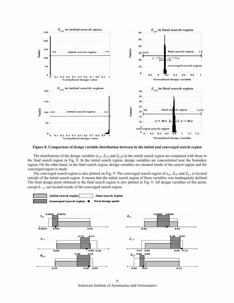
Figure 8. Comparison of design variable distribution between in the initial and converged search region

The distributions of the design variables (rLE, ZUP and ZLO) in the initial search region are compared with those in

the final search region in Fig. 8. In the initial search region, design variables are concentrated near the boundary region. On the other hand, in the final search region, design variables are situated inside of the search region and the converged region is made.

The converged search region is also plotted on Fig. 9. The converged search region of rLE, ZUP and ZLO is located outside of the initial search region. It means that the initial search region of these variables was inadequately defined. The final design point obtained in the final search region is also plotted in Fig. 9. All design variables of this point, except βTE, are located inside of the converged search region.

American Institute of Aeronautics and Astronautics

9

Figure 9. The converged search region

In order to identify the effect of each design variable to the lift and the drag coefficients, the ANOVA is

performed to both the initial search region and the final search region. Design variables and their interactions whose proportion to the total variance is over than 2.0% are shown in Fig. 10.

(a) Initial search region

(b) Final search region

Figure 10. ANOVA results in the initial search region and the final search region. According to the results, ZUP and ZLO are important design variables in both the initial and final search regions. rLE which was not so important in the initial search region becomes important in the final search region. Thus, the elimination of a design variable without the validity check of the search region may bring about an undesirable design result. In the final search region, design variable βTE has little effect on both the lift and the drag coefficient. This is the reason why βTE of the final design point is deviated from the converged search region. BecauseβTE is not so important design variable for the present design problem, the final design point is found outside of the converged search region ofβTE.

The geometry and pressure distribution of the designed airfoil (final design point) are shown in Fig. 11. The airfoil whose drag coefficient is smallest while satisfying the constraints is selected from the non-dominated

American Institute of Aeronautics and Astronautics

10

solutions of the MOGA. The aerodynamic performance and cross-sectional area of the design are compared with those of RAE2822 in Table 2. While satisfying the constraints, the drag coefficient of the designed airfoil is significantly decreased. Strong shock on the upper surface of RAE2822 airfoil has disappeared. These values are also compared with the result of the fixed search region case16 including the final design point. CL-fixed (=Cl_RAE2822) calculations are also performed for two designed airfoils. The pressure distributions are shown in Fig.12 and the aerodynamic performances are compared in the Table 3.

Table 2. Comparison of aerodynamic performance and cross-section area of airfoils

CL CD L/D AREA

RAE2822 0.7534 0.01687 44.65 0.0777 Design

(Present method) 0.7632 0.01410 54.12 0.0779 Design

(Fixed search region) 0.7827 0.01420 54.80 0.0783

Figure 11. Geometry and pressure distribution of the designed airfoil

Figure 12. Comparison of pressure distribution at the fixed CL condition(Cl=0.7534)

Table 3. Comparison of aerodynamic performance

CL CD L/D Design

(Present method) AOA = 2.650

0.7534 0.01398 53.87

Design (Fixed search region)

AOA=2.557 0.7534 0.01406 53.54

Even with the inadequate initial design space, an airfoil which has a good aerodynamic performance can be obtained by the change of search region.

American Institute of Aeronautics and Astronautics

11

VII. Conclusion In this paper, Kriging model was applied t onstrai ective optimization problem. The model was

constructed for each constraint and objectiv io ng model for the drag coefficient, the expected imp

on was modified. Functional analysis of variance (ANOVA) was

References 1 Myers, R. H. and Montgomery, D. C, Response Surface M : Process and Product Optimization Using Designed

Experiments, John Wiley & Sons, New York, 1995.

o a c ned multi-obje funct n. In the Krigi

rovement was calculated. In the Kriging model for the lift coefficient, the probability of satisfying the constraint was calculated. Based on these values, additional sample points for the balanced local and global search were selected successively, while satisfying the constraints.

During the optimization process, the validity of the search region was examined by investigating the distribution of design variables. Based on this result, the search regi

performed in both the initial and final search region to identify which design variables are important for objective and constraint functions. The results showed that the elimination of a design variable without the validity check of the search region may bring about an undesirable design result. Even with the inadequate initial design space, an airfoil which has a good aerodynamic performance can be obtained by using the present method.

ethodology

2Timothy, W. S., Timothy M. M., John, J. K. and Farrokh, M, “Comparison of Response Surface And Kriging Models for Multidisciplinary Design Optimization,” AIAA paper 98-4755.

3Sack, J., Welch, W. J., Mitchell, T. J. and Wynn, H. P., “Design and analysis of computer experiments (with discussion),” Statistical Science 4, 1989, pp. 409-435.

4Matthias, S., William, J. W. and Donald, R. J., “Global Versus Local Search in Constrained Optimization of Computer Models,” New Developments and Applications in Experimental Design, edited by N. Flournoy, W.F. Rosenberger, and W.K. Wong , Institute of Mathematical Statistics, Hayward, California, Vol. 34, 1998, pp. 11-25.

5Donald, R. J., Matthias S and William J. W, “Efficient Global Optimization of Expensive Black-Box Function,” Journal of global optimization, Vol. 13, 1998, pp. 455-492.

6Shinkyu, J., Mitsuhiro, M. and Kazuomi Y., “Efficient Optimization Design Method Using Kriging Model,” AIAA paper 2004-0118.

7Koehler, J and Owen, A. Computer experiments, in S. Ghosh and C. R. Rao (eds.), Handbook of Statistics, 13: Design and Analysis of Experiments, Elsevier, Amsterdam, 1996, pp. 261-308.

8Mardia, K. V. and R. J. Marshall, “Maximum likelihood estimation of models for residual covariance in Spatial regression,” Biometrika Vol. 71, 1984, pp. 135-146.

9Matthias, S., “Computer Experiments and Global Optimization,” Ph.D Dissertation, Statistic and Actuarial Science Dept., University of Waterloo, Waterloo, Ontario, 1997.

10Goldberg, D. E., “Genetic Algorithms in Search, Optimization & Machine Learning,” Addison-Wesley Publishing, Inc., Reading, Jan., 1989.

11Sobieczky, H., “Parametric Airfoils and Wings,” Recent Development of Aerodynamic Design Methodologies -Inverse Design and Optimization-, edited by Fuji, K. and Dulikaravich, G. S., Friedr. Vieweg & Sohn Verlagsgesellschaft mbH, Braunschweig/Wiesbaden, 1999, pp. 71-87.

12Owen, A. B., “Orthogonal arrays for computer experiments, integration and visualization,” Statistica Sinica, Vol. 2, 1992, pp. 439-452.

13Mckay, M. D., Beckman, R. J. and Conover, W. J., “A Comparison of Three Methods for Selecting Values of Input Variales in the Analysis of Output from a Computer Code,” Technometric, Vol. 21, No. 2, 1979, pp. 239-245.

14Obayashi, S. and Guruswamy, G. P., “Convergence Acceleration of a Aeroelastic Navier-Stokes Solver,” AIAA Journal, Vol. 33, No. 6, 1995, pp. 1134-1141.

15Takami, H., Kita, H., and Kobayashi, S., “Multi-Objective Optimization by Genetic Algorithms: A Review,” Proceedings of 1996 IEEE International Conference on Evolutionary Computation, 1996, pp. 517-522.

16Shinkyu, J., “Efficient and Robust Constraint Optimization of Aerodynamic Design with Kriging Model,” Proceedings of International Conference on Nonlinear Problems on Aviation and Aerospace 2004. (to be published)

American Institute of Aeronautics and Astronautics

12