100
Statistical Process Control Kvalitetsflow 2015 1

Statistical
Process ControlKvalitetsflow 2015
1
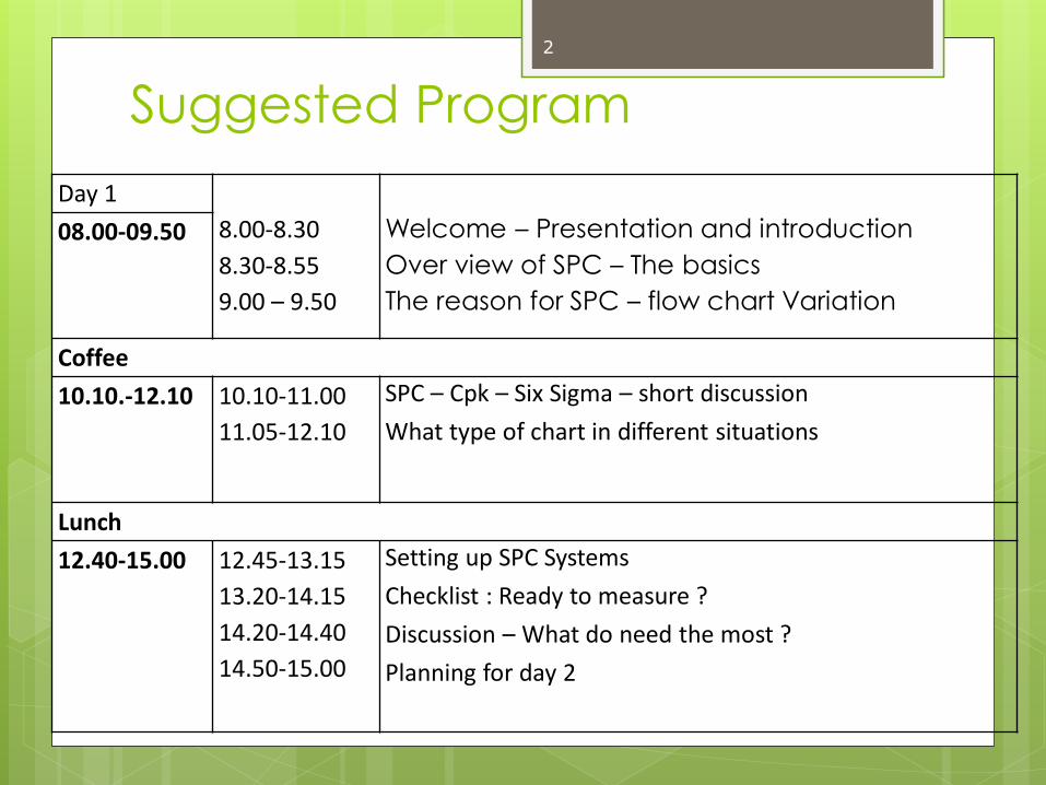
Suggested Program
Day 1
8.00-8.30
8.30-8.55
9.00 – 9.50
Welcome – Presentation and introduction
Over view of SPC – The basics
The reason for SPC – flow chart Variation
08.00-09.50
Coffee
10.10.-12.10 10.10-11.00
11.05-12.10
SPC – Cpk – Six Sigma – short discussion
What type of chart in different situations
Lunch
12.40-15.00 12.45-13.15
13.20-14.15
14.20-14.40
14.50-15.00
Setting up SPC Systems
Checklist : Ready to measure ?
Discussion – What do need the most ?
Planning for day 2
2

Suggested Program
Day 2
8.00-8.30
8.30-8.55
9.00 – 9.50
Setting up SPC in QDA
Make QDA fit to your data
Case: try it on your data
08.00-09.50
Coffee
10.10.-12.10 10.10-11.00
11.05-12.10
Case: try it on your data
Analysis and reporting
Lunch
12.40-15.00 12.45-13.15
13.20-14.15
14.20-14.40
14.50-15.00
Analysis and reporting
Additional theory?
Analysis on your data – setting up reports
Evaluation and actions agreed
3

Training in SPC
and Setting up
SPC in QDA
4

Setting up a SPC in general
Proces variables – how to find the relationbetween the proces variables and our SPC measure system.
First things first – MSA (Measure system analysis) to approve the system before we collect all data make decision on ”shaky ground”
Collecting basic information about the proces
USL, LSL
UCL, LCL
CP and Cpk values and targets
5
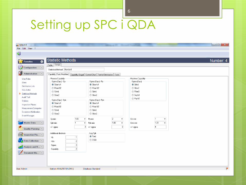
Setting up SPC i QDA
6

Six Sigma as a Metric
Sigma = = Deviation( Square root of variance )
-7 -6 -5 -4 -3 -2 -1 0 1 2 3 4 5 6 7
Axis graduated in Sigma
68.27 %
95.45 %
99.73 %
99.9937 %
99.999943 %
99.9999998 %
result: 317300 ppm outside
(deviation)
45500 ppm
2700 ppm
63 ppm
0.57 ppm
0.002 ppm
between + / - 1
between + / - 2
between + / - 3
between + / - 4
between + / - 5
between + / - 6
7
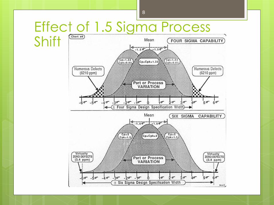
Effect of 1.5 Sigma Process Shift
8
Drift and combinations of PPM
and sigma
9
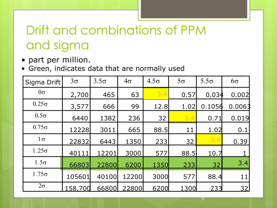
• part per million.• Green, indicates data that are normally used
Sigma Drift 3 3.5 4 4.5 5 5.5 6
0 2,700 465 63 0.57 0.034 0.002
0.25 3,577 666 99 12.8 1.02 0.1056 0.0063
0.5 6440 1382 236 32 3.4 0.71 0.019
0.75 12228 3011 665 88.5 11 1.02 0.1
1 22832 6443 1350 233 32 3.4 0.39
1.25 40111 12201 3000 577 88.5 10.7 1
1.5 66803 22800 6200 1350 233 32 3.4
1.75 105601 40100 12200 3000 577 88.4 11
2 158,700 66800 22800 6200 1300 233 32
3.4
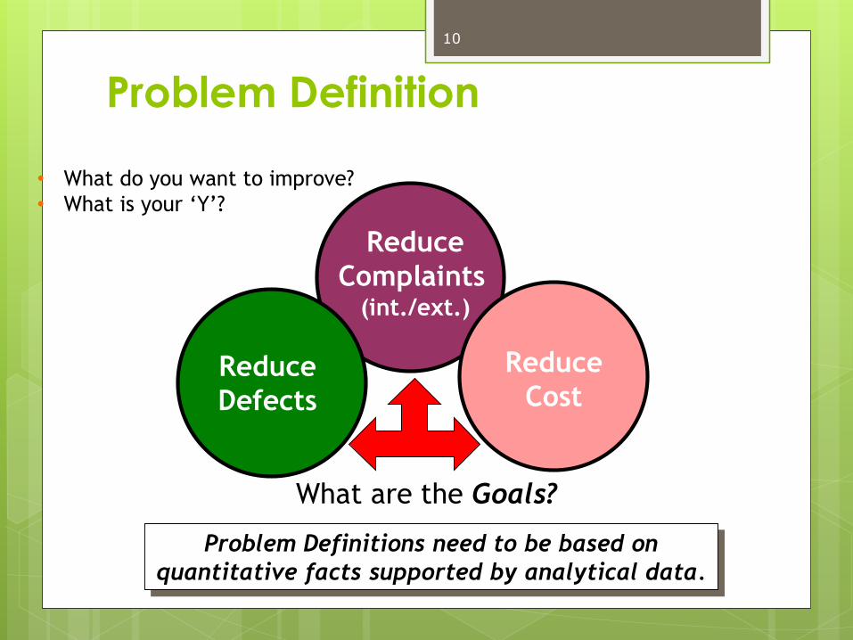
Reduce
Complaints(int./ext.)
Reduce
CostReduce
Defects
Problem Definitions need to be based on
quantitative facts supported by analytical data.
What are the Goals?
• What do you want to improve?
• What is your ‘Y’?
Problem Definition
10

To understand where you want to
be, you need to know how to get
there.
Map the Process
Measure the Process
Identify the variables - ‘x’
Understand the Problem -
’Y’ = function of variables -’x’
Y=f(x)
11
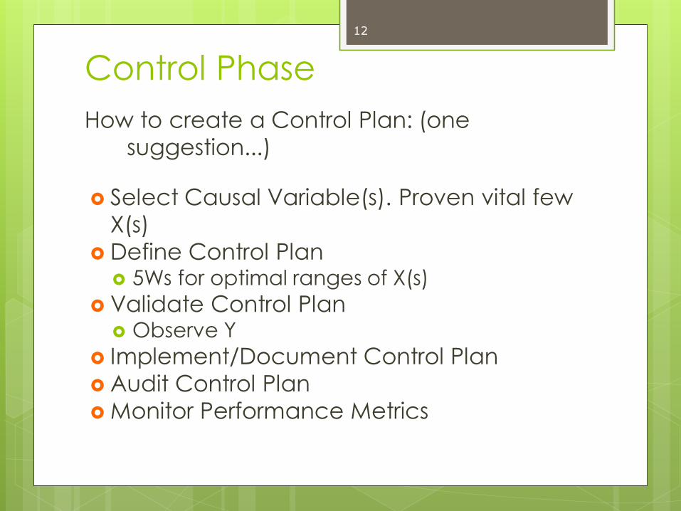
Control Phase
How to create a Control Plan: (one
suggestion...)
Select Causal Variable(s). Proven vital few
X(s)
Define Control Plan 5Ws for optimal ranges of X(s)
Validate Control Plan Observe Y
Implement/Document Control Plan
Audit Control Plan
Monitor Performance Metrics
12

Control Phase
Control Plan Tools:
Statistical Process Control (SPC)
Used with various types of distributions
Control Charts
Attribute based (np, p, c, u). Variable based (X-R, X)
Additional Variable based tools
-PRE-Control
-Common Cause Chart (Exponentially Balanced
Moving Average (EWMA))
13
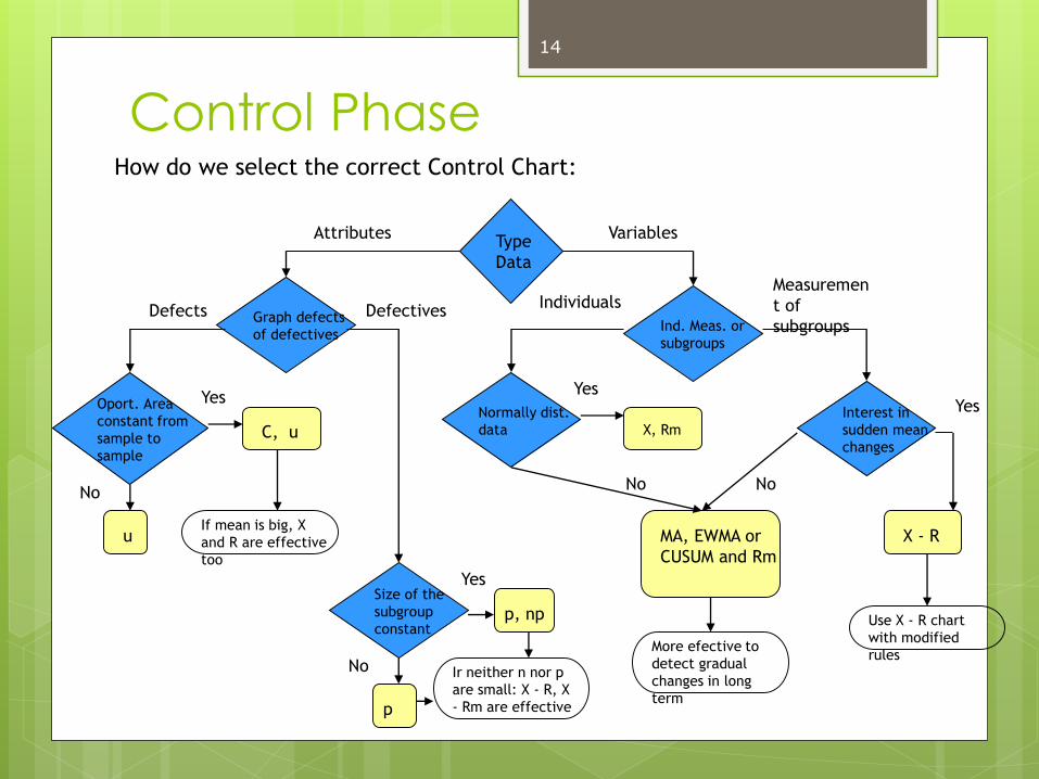
Control PhaseHow do we select the correct Control Chart:
Type
Data
Ind. Meas. or
subgroups
Normally dist.
data
Interest in
sudden mean
changes
Graph defects
of defectives
Oport. Area
constant from
sample to
sample
X, Rm
p, np
X - RMA, EWMA or
CUSUM and Rm
u
C, u
Size of the
subgroup
constant
p
If mean is big, X
and R are effective
too
Ir neither n nor p
are small: X - R, X
- Rm are effective
More efective to
detect gradual
changes in long
term
Use X - R chart
with modified
rules
VariablesAttributes
Measuremen
t of
subgroups
Individuals
Yes
No No
Yes
Yes
No
Yes
No
Defects Defectives
14
15

Statistical Process Control
(SPC)
Invented by Walter Shewhart at Western
Electric
Distinguishes between
common cause variability (random)
special cause variability (assignable)
Based on repeated samples from a
process
16

Statistical Process Control
(SPC)
A methodology for monitoring a process
to identify special causes of variation and
signal the need to take corrective action
when appropriate
SPC relies on control charts
17

Variability
Deviation = distance between
observations and the mean (or
average)
Results for “Emmett”
Emmett
Jake
Observations
10
9
8
8
7
averages 8.4
Deviations
10 - 8.4 = 1.6
9 – 8.4 = 0.6
8 – 8.4 = -0.4
8 – 8.4 = -0.4
7 – 8.4 = -1.4
0.0
8
7
10
8
9
18

Variability
Deviation = distance between
observations and the mean (or average)
Results for “Jake”
Emmett
Jake
Observations
7
7
7
6
6
averages 6.6
Deviations
7 – 6.6 = 0.4
7 – 6.6 = 0.4
7 – 6.6 = 0.4
6 – 6.6 = -0.6
6 – 6.6 = -0.6
0.0
7
6
7
7
6
19

Variability
Variance = average distance between
observations and the mean squared
Emmett
Jake
Observations
10
9
8
8
7
averages 8.4
Deviations
10 - 8.4 = 1.6
9 – 8.4 = 0.6
8 – 8.4 = -0.4
8 – 8.4 = -0.4
7 – 8.4 = -1.4
0.0
8
7
10
8
9
Squared Deviations
2.56
0.36
0.16
0.16
1.96
1.0 Variance
20

Variability
Variance = average distance between
observations and the mean squared
Emmett
Jake
Observations
7
7
7
6
6
averages
Deviations Squared Deviations
7
6
7
7
6
21

Variability
Variance = average distance between
observations and the mean squared
Emmett
Jake
Observations
7
7
7
6
6
averages 6.6
Deviations
7 - 6.6 = 0.4
7 - 6.6 = 0.4
7 - 6.6 = 0.4
6 – 6.6 = -0.6
6 – 6.6 = -0.6
0.0
Squared Deviations
0.16
0.16
0.16
0.36
0.36
0.24
7
6
7
7
6
Variance
22

Variability
Standard deviation = square root of
variance
Emmett
Jake
Variance Standard Deviation
Emmett 1.0 1.0
Jake 0.24 0.4898979
23

VariabilityThe world tends to be bell-shaped
Most outcomes
occur in the
middleFewer
in the
“tails”
(lower)
Fewer
in the
“tails”
(upper)
Even very rare
outcomes are
possible
(probability > 0)
Even very rare
outcomes are
possible
(probability > 0)
24
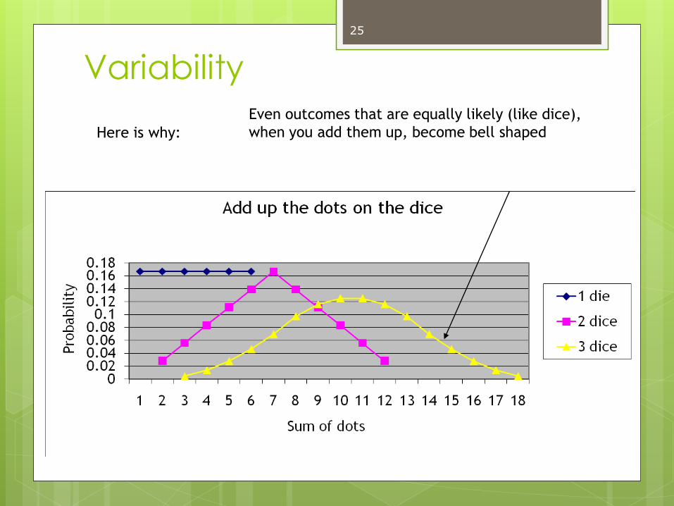
Variability
Here is why:
Even outcomes that are equally likely (like dice),
when you add them up, become bell shaped
25
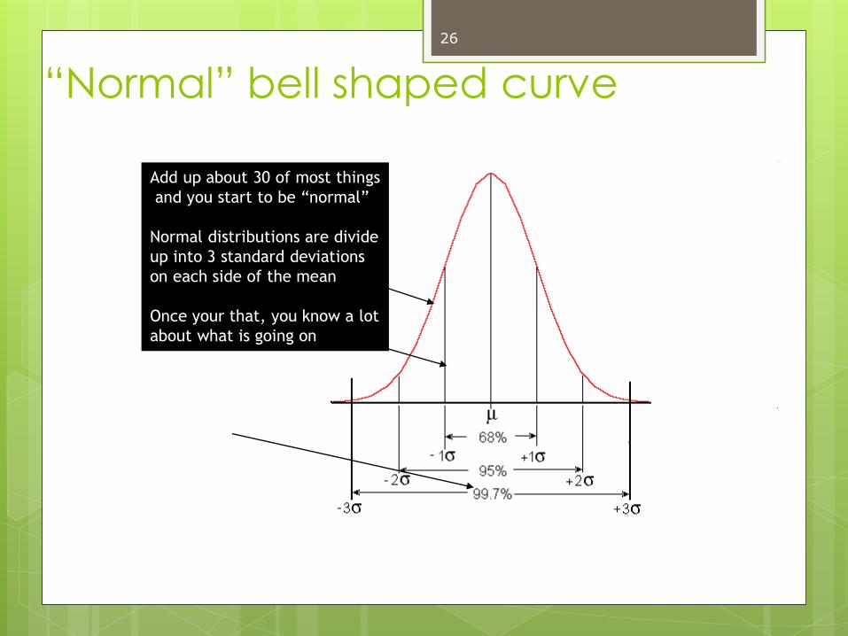
“Normal” bell shaped curve
Add up about 30 of most things
and you start to be “normal”
Normal distributions are divide
up into 3 standard deviations
on each side of the mean
Once your that, you know a lot
about what is going on
26

Causes of Variability
Common Causes:
Random variation (usual)
No pattern
Inherent in process
adjusting the process increases its variation
Special Causes
Non-random variation (unusual)
May exhibit a pattern
Assignable, explainable, controllable
adjusting the process decreases its variation
27

Process
mean
Lower
specification
Upper
specification
1350 ppm 1350 ppm
1.7 ppm 1.7 ppm
+/- 3 Sigma
+/- 6 Sigma
3 Sigma and 6 Sigma Quality
28

Statistical Process Control
The Control Process
Define
Measure
Compare
Evaluate
Correct
Monitor results
Variations and Control
Random variation: Natural variations in the output of a process, created by countless minor factors
Assignable variation: A variation whose source can be identified
29

Sampling Distribution
Sampling
distribution
Process
distribution
Mean
30

Normal Distribution
Mean3 2 2 3
95.44%
99.74%
Standard deviation
31

Control LimitsSampling
distribution
Process
distribution
Mean
Lower
control
limit
Upper
control
limit
32

SPC Errors
Type I error
Concluding a process is not in control when it actually is.
Type II error
Concluding a process is in control when it is not.
33

Type I Error
Mean
LCL UCL
/2 /2
Probability
of Type I error
34
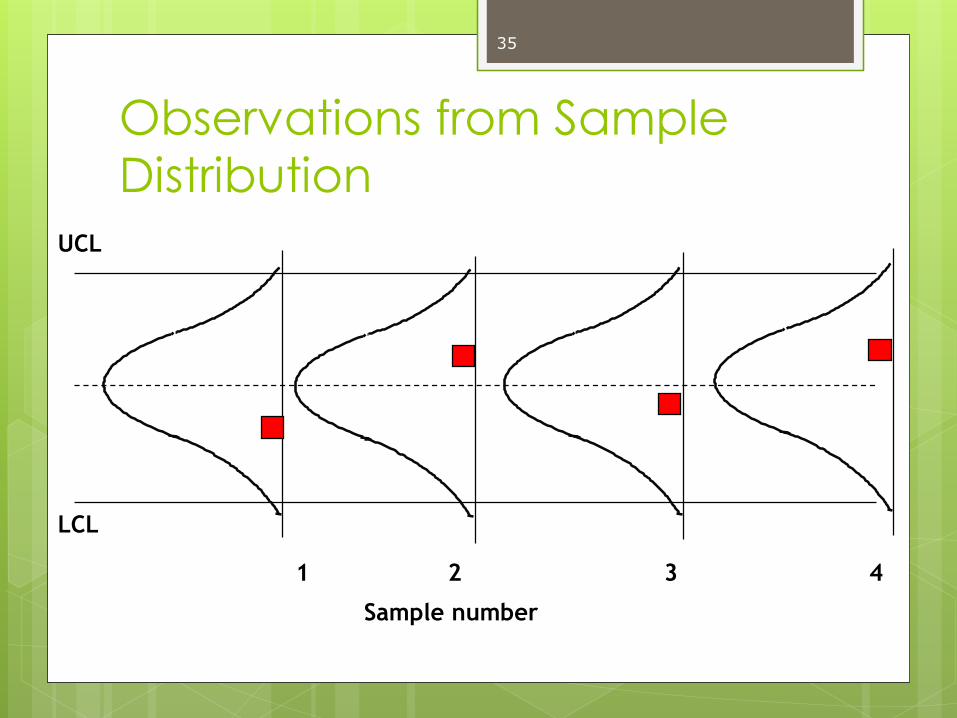
Observations from Sample
Distribution
Sample number
UCL
LCL
1 2 3 4
35
Control Chart
Control Chart
Purpose: to monitor process output to see if it is random
A time ordered plot representative sample statistics obtained from an on going process (e.g. sample means)
Upper and lower control limits define the range of acceptable variation
36
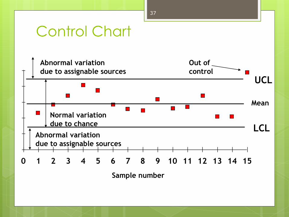
Control Chart
0 1 2 3 4 5 6 7 8 9 10 11 12 13 14 15
UCL
LCL
Sample number
Mean
Out of
control
Normal variation
due to chance
Abnormal variation
due to assignable sources
Abnormal variation
due to assignable sources
37

Control Charts in General
Are named according to the statistics
being plotted, i.e., X bar, R, p, and c
Have a center line that is the overall
average
Have limits above and below the center
line at ± 3 standard deviations (usually)
Center line
Lower Control Limit (LCL)
Upper Control Limit (UCL)
38
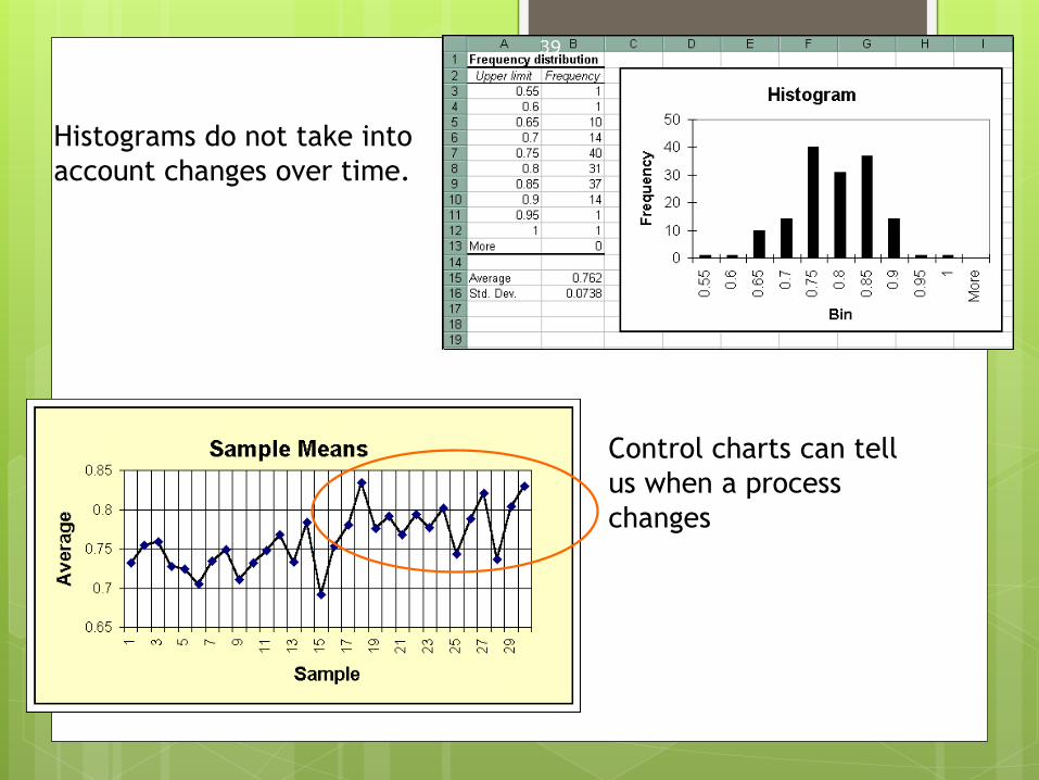
Histograms do not take into
account changes over time.
Control charts can tell
us when a process
changes
39
Control Chart Applications
Establish state of statistical control
Monitor a process and signal when it goes
out of control
Determine process capability
40

Commonly Used Control
Charts
Variables data
x-bar and R-charts
x-bar and s-charts
Charts for individuals (x-charts)
Attribute data
For “defectives” (p-chart, np-chart)
For “defects” (c-chart, u-chart)
41
Developing Control Charts
Prepare
Choose measurement
Determine how to collect data, sample size, and frequency of sampling
Set up an initial control chart
Collect Data
Record data
Calculate appropriate statistics
Plot statistics on chart
42
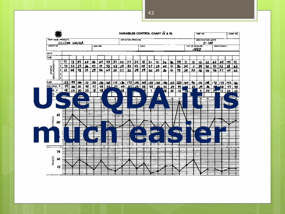
43
Use QDA it is much easier

Next Steps
Determine trial control limits
Center line (process average)
Compute UCL, LCL
Analyze and interpret results
Determine if in control
Eliminate out-of-control points
Recompute control limits as necessary
44
Limits
Process and Control limits:
Statistical
Process limits are used for individual items
Control limits are used with averages
Limits = μ ± 3σ
Define usual (common causes) & unusual (special causes)
Specification limits:
Engineered
Limits = target ± tolerance
Define acceptable & unacceptable
45
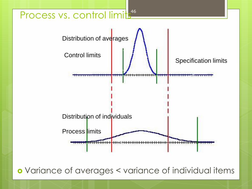
Process vs. control limits
Variance of averages < variance of individual items
Distribution of averages
Control limits
Process limits
Distribution of individuals
Specification limits
46

Variables Data Charts
Process Centering
X bar chart
X bar is a sample mean
Process Dispersion (consistency)
R chart
R is a sample range
n
X
X
n
i
i 1
)min()max( ii XXR
47

X bar charts
Center line is the grand mean (X double
bar)
Points are X bars
xzXUCL
nx
/
xzXLCL
m
X
X
m
j
j
1
RAXUCL 2 RAXLCL 2
-OR-
48

R Charts
Center line is the grand mean (R bar)
Points are R
D3 and D4 values are tabled according
to n (sample size)
RDUCL 4 RDLCL 3
49

Use of X bar & R charts
Charts are always used in tandem
Data are collected (20-25 samples)
Sample statistics are computed
All data are plotted on the 2 charts
Charts are examined for randomness
If random, then limits are used “forever”
50

Attribute Charts
c charts – used to
count defects in a
constant sample sizecenterline
m
c
c
n
i 1
czcUCL
czcLCL

Attribute Charts
p charts – used to track
a proportion (fraction)
defective
n
x
p
n
i
i
i
1centerline
nm
x
m
p
p ij
m
j
1
n
ppzpUCL
)1(
n
ppzpLCL
)1(

Control Charts for Variables
Mean control charts
Used to monitor the central tendency of a process.
X bar charts
Range control charts
Used to monitor the process dispersion
R charts
Variables generate data that are measured.
53

Mean and Range Charts
UCL
LCL
UCL
LCL
R-chart
x-Chart Detects shift
Does not
detect shift
(process mean is
shifting upward)Sampling
Distribution
54

Mean and Range Charts
x-Chart
UCL
Does not
reveal increase
UCL
LCL
LCL
R-chart Reveals increase
(process variability is increasing)Sampling
Distribution
55

Control Chart for Attributes
p-Chart - Control chart used to monitor
the proportion of defectives in a process
c-Chart - Control chart used to monitor
the number of defects per unit
Attributes generate data that are counted.
56
Use of p-Charts
When observations can be placed into
two categories.
Good or bad
Pass or fail
Operate or don’t operate
When the data consists of multiple
samples of several observations each
57

Use of c-Charts
Use only when the number of
occurrences per unit of measure can be
counted; non-occurrences cannot be
counted.
Scratches, chips, dents, or errors per item
Cracks or faults per unit of distance
Breaks or Tears per unit of area
Bacteria or pollutants per unit of volume
Calls, complaints, failures per unit of time
58

Use of Control Charts
At what point in the process to use control
charts
What size samples to take
What type of control chart to use
Variables
Attributes
59

Run Tests
Run test – a test for randomness
Any sort of pattern in the data would
suggest a non-random process
All points are within the control limits - the
process may not be random
60
Nonrandom Patterns in Control charts
Trend
Cycles
Bias
Mean shift
Too much dispersion
61

Typical Out-of-Control Patterns
Point outside control limits
Sudden shift in process average
Cycles
Trends
Hugging the center line
Hugging the control limits
Instability
62

Shift in Process Average
63
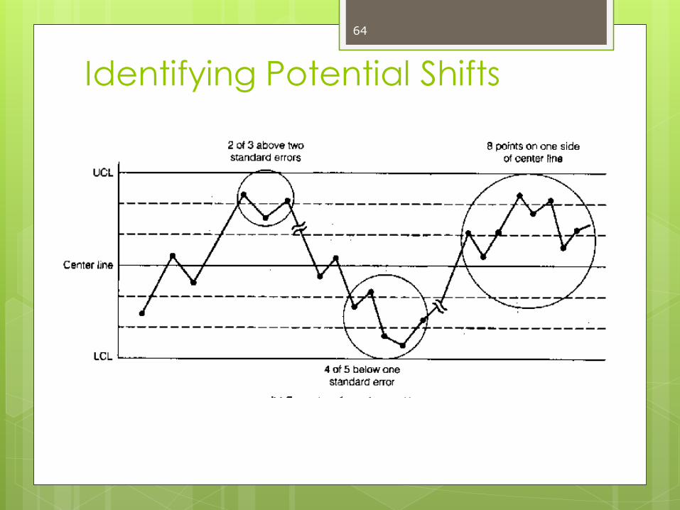
Identifying Potential Shifts
64

Cycles
65

Trend
66

Final Steps
Use as a problem-solving tool
Continue to collect and plot data
Take corrective action when necessary
Compute process capability
67

Process Capability
Tolerances or specifications
Range of acceptable values established by engineering design or customer requirements
Process variability
Natural variability in a process
Process capability
Process variability relative to specification
68

Process CapabilityLower
SpecificationUpper
Specification
A. Process variability
matches specificationsLower
Specification
Upper
Specification
B. Process variability
well within specificationsLower
Specification
Upper
Specification
C. Process variability
exceeds specifications
69

Process Capability Ratio
70
Process capability ratio, Cp =specification width
process width
Upper specification – lower specification
6Cp =

Improving Process Capability
Simplify
Standardize
Mistake-proof
Upgrade equipment
Automate
71

Taguchi Loss Function
Cost
TargetLower
specUpper
spec
Traditional
cost function
Taguchi
cost function
72

Meet the Guru: Taguchi
Taguchi
Quality through design
1) Product must bee robust to variation in process
2) Loss is equal to distance from nominal
The ”old” philosophy Lower tolerance Upper tolerance
The ”Taguchi” philosophyLower tolerance Upper tolerance
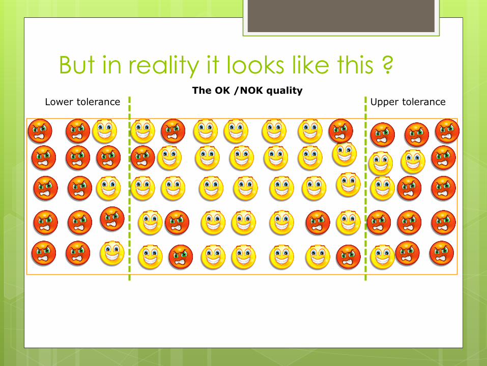
But in reality it looks like this ?The OK /NOK quality
Lower tolerance Upper tolerance
Limitations of Capability
Indexes
Process may not be stable
Process output may not be normally
distributed
Process not centered but Cp is used
75

Process Capability
The ratio of process
variability to design
specifications
Text Text Text Text Text Text
Title
Upper
Spec
Lower
Spec
Natural data
spread
The natural
spread of the
data is 6σ
-
1σ+2σ-2σ +1σ +3σ-3σ µ

Empirical Rule
-3 -1-2 +1 +2 +3
68%
95%
99.7%
77
Gauges and Measuring Instruments
Variable gauges
Fixed gauges
Coordinate measuring machine
Vision systems
78

Examples of Gauges
79

Metrology - Science of
Measurement• Accuracy - closeness of agreement
between an observed value and a
standard
• Precision - closeness of agreement
between randomly selected individual
measurements
80

Repeatability and
Reproducibility
Repeatability (equipment variation) –
variation in multiple measurements by an
individual using the same instrument.
Reproducibility (operator variation) -
variation in the same measuring
instrument used by different individuals
81

Repeatability and
Reproducibility Studies
Quantify and evaluate the capability of a
measurement system
Select m operators and n parts
Calibrate the measuring instrument
Randomly measure each part by each operator for r trials
Compute key statistics to quantify repeatability and reproducibility
82

Reliability and Reproducibility
Studies(2)
all of range average
operatoreach for range average
operatoreach for part each for range )(min)(maxR
averagesoperator of (range) difference )(min)(max
operatoreach for average
r) to1 from(k Trials
in n) to1 from (j Parts
on m) to1 from (i Operators
by made (M)t Measuremen
ij
m
R
R
n
R
R
MM
xxx
rn
M
x
i
i
j
ij
i
ijkk
ijkk
ii
ii
D
j k
ijk
i
83
Use QDA it is much easier
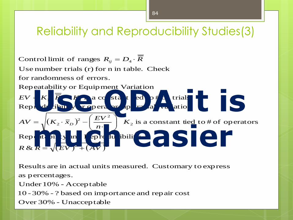
Reliability and Reproducibility Studies(3)
ble Unaccepta- 30%Over
costrepair and importanceon based ? - 30%-10
Acceptable - 10%Under
s.percentage as
express toCustomary measured. units actualin are Results
&
ilityReproducib andity Repeatabil
operators of # toiedconstant t a is
variation)(appraisaloperator or ility Reproducib
trialsof # toiedconstant t a is
VariationEquipment or ity Repeatabil
errors. of randomnessfor
Check in table.n for (r) alsnumber tri Use
ranges oflimit Control
22
2
22
2
11
4
AVEVRR
Krn
EVxKAV
KRKEV
RDR
D
ij
84
Use QDA it is much easier
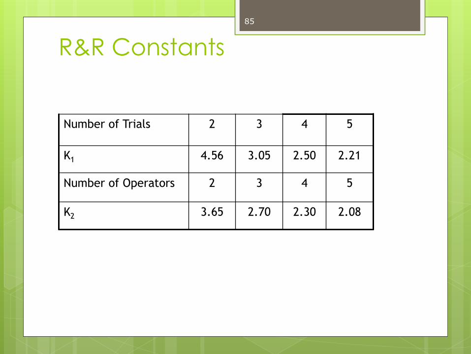
R&R Constants
Number of Trials 2 3 4 5
K1 4.56 3.05 2.50 2.21
Number of Operators 2 3 4 5
K2 3.65 2.70 2.30 2.08
85

R&R Evaluation
Under 10% error - OK
10-30% error - may be OK
over 30% error - unacceptable
86

Process Map
Historical Data
Fishbone
How do we know our process?
87

RATIONAL SUBROUPING Allows samples to be taken that
include only white noise, within the samples. Black noise
occurs between the samples.
RATIONAL SUBGROUPS
Minimize variation within subgroups
Maximize variation between subgroups
TIME
PRO
CESS
RESPO
NSE
WHITE NOISE
(Common Cause
Variation)
BLACK NOISE
(Signal)
88

Visualizing the Causes
st + shift =
total
Time 1
Time 2
Time 3
Time 4
Within Group
•Called short term (sst)
•Our potential – the best we can be
•The s reported by all 6 sigma companies
•The trivial many
89
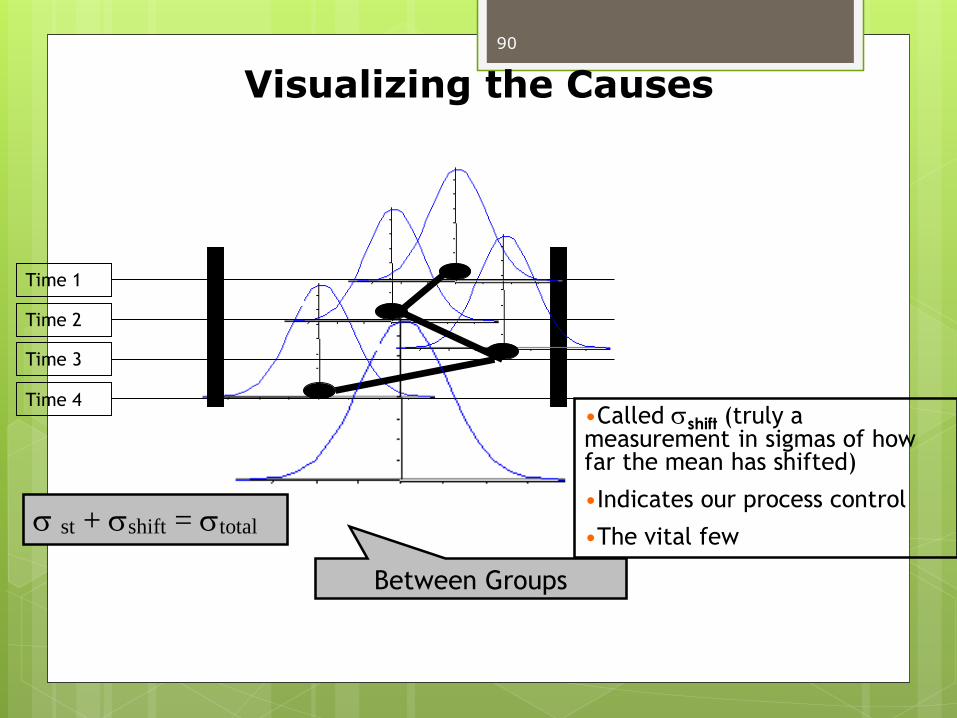
Visualizing the Causes
Between Groups
st + shift = total
Time 1
Time 2
Time 3
Time 4•Called shift (truly a measurement in sigmas of how far the mean has shifted)
•Indicates our process control
•The vital few
90

Assignable Cause
Outside influences
Black noise
Potentially controllable
How the process is actually performing
over time
Fishbone
91

Common Cause Variation
Variation present in every process
Not controllable
The best the process can be within the
present technology
92
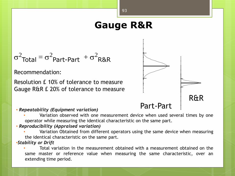
2Total = 2
Part-Part + 2R&R
Recommendation:
Resolution £ 10% of tolerance to measure
Gauge R&R £ 20% of tolerance to measure
• Repeatability (Equipment variation)
• Variation observed with one measurement device when used several times by one
operator while measuring the identical characteristic on the same part.
• Reproducibility (Appraised variation)
• Variation Obtained from different operators using the same device when measuring
the identical characteristic on the same part.
•Stability or Drift
• Total variation in the measurement obtained with a measurement obtained on the
same master or reference value when measuring the same characteristic, over an
extending time period.
Gauge R&R
Part-PartR&R
93
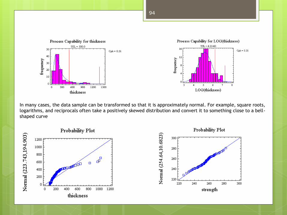
In many cases, the data sample can be transformed so that it is approximately normal. For example, square roots,
logarithms, and reciprocals often take a positively skewed distribution and convert it to something close to a bell-
shaped curve
94

LSL USL LSL USL
LSL USL
Off-Target, Low Variation
High Potential Defects
Good Cp but Bad Cpk
On Target
High Variation
High Potential Defects
No so good Cp and Cpk
On-Target, Low Variation
Low Potential Defects
Good Cp and Cpk
Variation reduction and process
centering create processes with
less potential for defects.
The concept of defect reduction
applies to ALL processes (not just
manufacturing)
What do we Need?
95

Eliminate “Trivial Many”
• Qualitative Evaluation
• Technical Expertise
• Graphical Methods
• Screening Design of Experiments Identify “Vital Few”
• Pareto Analysis
• Hypothesis Testing
• Regression
• Design of ExperimentsQuantify
Opportunity
• % Reduction in Variation
• Cost/ BenefitOur Goal:
Identify the Key Factors (x’s)
96
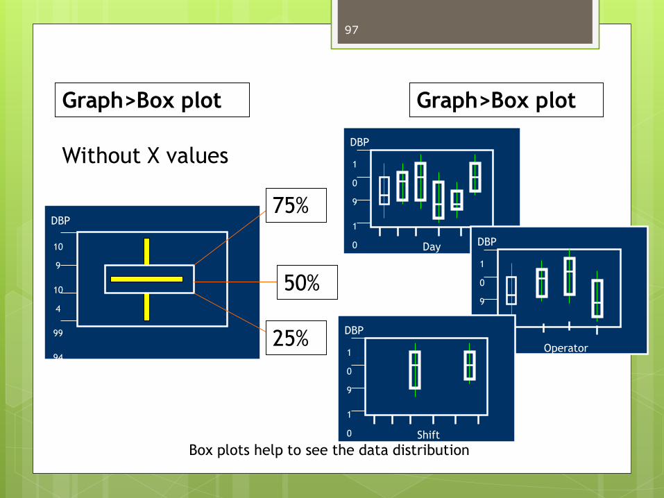
Graph>Box plot
75%
50%
25%
Graph>Box plot
Without X values
DBP
Box plots help to see the data distribution
Day
DBP
1
0
9
1
0
4
9
9
9
4
10
9
10
4
99
94Operator
DBP
1
0
9
1
0
4
9
9
9
4
Shift
DBP
1
0
9
1
0
97

Statistical Analysis
0.0250.0200.0150.0100.0050.000
7
6
5
4
3
2
1
0
New Machine
Fre
que
ncy
0.0250.0200.0150.0100.0050.000
30
20
10
0
Machine 6 mthsF
req
ue
ncy
• Is the factor really important?
• Do we understand the impact for
the factor?
• Has our improvement made an
impact
• What is the true impact?
Hypothesis Testing
Regression Analysis
5545352515 5
60
50
40
30
20
10
0
X
Y
R-Sq = 86.0 %
Y = 2.19469 + 0.918549X
95% PI
Regression
Regression Plot
Apply statistics to validate actions & improvements
98

Con-sumer Cue
Technical Requirement
Preliminary Drawing/DatabaseIdentity CTQs
Identify Critical Process
Obtain Data on Similar Process
Calculate Z values
Rev 0 Drawings
Stop Adjust process & design
1st piece inspection
Prepilot Data
Pilot data
Obtain data
Recheck ‘Z’ levels
Stop Fix process & design
Z<3
Z>= Design Intent M.A.I.C
M.A.D
99

Excercise
100


