L IQUIDITY A FFECTS J OB C HOICE : E VIDENCE FROM T EACH F OR A MERICA * LUCAS C. COFFMAN † J OHN J. CONLON CLAYTON R. FEATHERSTONE J UDD B. KESSLER MAY 21, 2019 Can access to a few hundred dollars of liquidity affect the career choice of a recent college graduate? In a three-year field experiment with Teach For America (TFA), a prestigious teacher placement program, we randomly increase the financial packages offered to nearly 7,300 potential teachers who requested support for the transition into teaching. The first two years of the experiment reveal that while most applicants do not respond to a marginal $600 of grants or loans, those in the worst financial position respond by joining TFA at higher rates. We continue the experiment into the third year and self-replicate our results. For the highest need applicants, an extra $600 in loans, $600 in grants, and $1,200 in grants increase the likelihood of joining TFA by 12.2, 11.4, and 17.1 percentage points (or 20.0%, 18.7%, and 28.1%), respectively. Additional grant and loan dollars are equally effective, suggesting a liquidity mechanism. A follow-up survey bolsters the liquidity story and also shows that those pulled into teaching would have otherwise worked in private sector firms. JEL Codes: I21, J22, J45, J62, J68. * The authors thank their many partners at Teach For America: Demi Ross, Sean Waldheim, Alex Spangler, Lee Loyd, Johann von Hoffmann, Lauren Moxey, and Brigid Pena. They also thank Katherine B. Coffman, Tatiana Homonoff, Simon Jäger, Lisa Kahn, Charles Sprenger, and seminar participants at Boston College, Harvard Business School, the Economic Science Association meetings, and the Advances in Field Experiments conference. Finally, they thank Larry Katz and four anonymous referees. The experiment is registered on the AEA RCT Registry with ID AEARCTR-0004168. The authors are grateful for funding from the Wharton Behavioral Lab and the Center for Human Resources at Wharton. † Corresponding author: [email protected], Department of Economics, Harvard University
Transcript
LIQUIDITY AFFECTS JOB CHOICE:EVIDENCE FROM TEACH FOR AMERICA*
LUCAS C. COFFMAN†
JOHN J. CONLONCLAYTON R. FEATHERSTONE
JUDD B. KESSLER
MAY 21, 2019
Can access to a few hundred dollars of liquidity affect the career choice ofa recent college graduate? In a three-year field experiment with Teach ForAmerica (TFA), a prestigious teacher placement program, we randomly increasethe financial packages offered to nearly 7,300 potential teachers who requestedsupport for the transition into teaching. The first two years of the experimentreveal that while most applicants do not respond to a marginal $600 of grantsor loans, those in the worst financial position respond by joining TFA at higherrates. We continue the experiment into the third year and self-replicate ourresults. For the highest need applicants, an extra $600 in loans, $600 in grants,and $1,200 in grants increase the likelihood of joining TFA by 12.2, 11.4, and17.1 percentage points (or 20.0%, 18.7%, and 28.1%), respectively. Additionalgrant and loan dollars are equally effective, suggesting a liquidity mechanism. Afollow-up survey bolsters the liquidity story and also shows that those pulled intoteaching would have otherwise worked in private sector firms. JEL Codes: I21,J22, J45, J62, J68.
*The authors thank their many partners at Teach For America: Demi Ross, Sean Waldheim, AlexSpangler, Lee Loyd, Johann von Hoffmann, Lauren Moxey, and Brigid Pena. They also thank KatherineB. Coffman, Tatiana Homonoff, Simon Jäger, Lisa Kahn, Charles Sprenger, and seminar participants atBoston College, Harvard Business School, the Economic Science Association meetings, and the Advancesin Field Experiments conference. Finally, they thank Larry Katz and four anonymous referees. Theexperiment is registered on the AEA RCT Registry with ID AEARCTR-0004168. The authors are gratefulfor funding from the Wharton Behavioral Lab and the Center for Human Resources at Wharton.
†Corresponding author: [email protected], Department of Economics, Harvard University
I. INTRODUCTION
Taking a new job can come with large financial costs. While many private sector firms
offer signing bonuses or travel reimbursement to help cover these costs, the typical
public service job is unlikely to offer such benefits, leaving workers to finance their
own transitions.1 For example, an aspiring teacher who graduates college in May
and starts teaching in September will spend a few months without a paycheck while
potentially facing additional expenses associated with moving and getting ready to
teach. A key feature of many of these transition costs is that they demand immediate
liquidity at the time of transition.
To what extent does the need for liquidity affect whether individuals take public
service jobs like teaching? If all workers had access to credit at a reasonable expense,
concerns about liquidity would be mitigated, and those who wanted to become teach-
ers (or work in other public service jobs) would be able to finance their transitions.
Evidence suggests, however, that many Americans—even college graduates—are both
illiquid and credit constrained.2
In this paper, we investigate the role liquidity plays in the choice to become a
teacher by running a large, three-year field experiment with a highly selective non-
profit teacher placement program, Teach For America (TFA). TFA draws many of its
potential teachers from highly ranked colleges and universities. Given the caliber
of those admitted to TFA, one might expect that they are not subject to liquidity
constraints; consequently, finding these constraints are important for even a subset of
those admitted suggests that such concerns may be more widely prevalent.
We run our experiment in the context of TFA’s “transitional grants and loans”
(TGL) program. The program invites prospective teachers to apply for funding to
support their transitions into TFA by providing a battery of financial information
that TFA uses to assess need. TFA then offers a personalized package of grants and
no-interest loans to each applicant based on its estimate of what the applicant needs to
make the transition into teaching. Applicants who accept the funds from TFA receive
them in late May or June to cover costs faced during the summer before they begin.
1For example, the transition into teaching—the focus of this paper—is unlikely to be supported bysuch benefits. The most recent Schools and Staffing Survey (SASS) estimates that only 3.8% of schooldistricts in the United States offer teachers signing bonuses and only 2.6% offer funding to help coverexpenses related to relocation (Hansen, Quintero, and Feng 2018).
2According to the New York Federal Reserve’s 2017 Survey of Consumer Expectations, 32% ofAmerican adults (and 18% of college graduates) believe there is less than a 50% chance that they couldcome up with $2,000 in the next month. See also Hayashi (1985); Zeldes (1989); Jappelli (1990); Grossand Souleles (2002); Johnson, Parker, and Souleles (2006); and Brown, Scholz, and Seshadri (2011).
1
Our experiment randomly varies the grant and loan packages offered to TGL
program applicants. Applicants in our experiment either receive a control package
or, in our main treatments, a package that randomly includes an additional $600 in
loans or $600 in grants. Other treatments, added partway through the experiment,
randomly offered some applicants an additional $1,200 in grants or an additional
$1,800 in loans or grants. Across all treatments, “additional” funds were not tagged
as special—TGL applicants randomized to our treatment groups were simply offered
larger packages than they would have been offered if randomized to our control group.
We find that for the majority of TGL applicants, additional funding does not
impact their decision to become a teacher for TFA. However, for the “highest need”
applicants (the 10 percent predicted by TFA to be unable to provide any funding for
their transitions), both the additional grants and the additional loans have large,
statistically significant, positive effects on becoming a teacher for TFA.
The first two years of data revealed a heterogeneous treatment effect. While there
are numerous methods to address the empirical validity of heterogeneous treatment
effects, we had the opportunity to run our experiment for a third year, which gave us
the chance to “self-replicate” our results. As discussed in Section III, after the first
two years of the experiment, we adjusted our experimental design to account for the
heterogeneous treatment effects we had found, highlighting the role of the third year
as a replication. This self-replication succeeded, generating results nearly identical to
those from the first two years.
Across the three years of the experiment, we estimate that providing an extra $600
in loans, $600 in grants, and $1,200 in grants increases the likelihood the highest
need applicants become teachers for TFA by 12.2, 11.4, and 17.1 percentage points,
respectively. These treatment effects represent 20.0%, 18.7%, and 28.1% increases in
joining TFA on a base rate of 0.61 in the control group. These large treatment effects
arise even though the highest need applicants are offered substantial grant and loan
packages (averaging around $5,000 per applicant) in the control group.
The pattern of our experimental results, institutional details of the TGL program,
and results from a post-experiment survey all strongly suggest that our treatments
work through the liquidity they provide to applicants. First, consistent with a liquidity
mechanism, we find that additional grants and loans are equally effective at inducing
the highest need applicants to join TFA (even though loans have to be repaid over
the course of the TFA program and grants do not). Second, as described in Section II,
the formula TFA uses to determine TGL awards has a kink that systematically offers
control awards below estimated liquidity need to the highest need applicants. Indeed,
2
in a post-experiment survey of our experimental subjects—described in Section III.A—
a large majority of the highest need applicants receiving the TGL control award
report needing additional liquidity. Third, the highest need applicants have difficulty
accessing credit markets. While the vast majority of the these applicants reported
applying for credit when needed, over a quarter of those who applied for credit said
they were denied. The latter few points also help explain why applicants with less
need do not respond to the treatments—they are not subject to the kink, they are less
likely to report having unmet liquidity need, and they are denied credit less often.
The post-experiment survey also reveals that applicants induced to join TFA by
our treatments would have otherwise ended up in private sector jobs. That additional
funding generated more teachers overall suggests that liquidity need may be pre-
venting workers from becoming teachers or otherwise entering public service. It also
suggests that loans may be a particularly cost-effective policy lever to mitigate this
barrier. We discuss the policy implications of our findings—and how they compare to
existing programs to attract and retain teachers—in Section VII.
Along with having policy implications, our results make contributions to two
related literatures. First, we add to the literature that investigates how liquidity
constraints affect important life decisions, such as consumption choices (Agarwal, Liu,
and Souleles 2007; Johnson, Parker, and Souleles 2006) and educational investments
(Lochner and Monge-Naranjo 2012). The closest related work on how finances affect
job choice considers unemployment insurance (UI), which necessarily focuses on older
workers whose decisions are on the margins of both unemployment duration and
job choice. This work finds evidence that liquidity can indeed affect unemployment
duration (Chetty 2008). However, there is not a consensus on whether the liquid-
ity provided by UI affects post-unemployment earnings or job match quality.3 Our
experiment involves relatively young workers and finds that giving them access to
liquidity affects the type of jobs they take early in their careers. This margin may
be particularly important, since evidence suggests that first jobs can have life-long
consequences. For example, graduating in a recession not only affects short-run wages,
but has modest long-run effects on careers and earnings—effects that may be due to
the quality of job match (see Kahn 2010; Oreopoulos, von Wachter, and Heisz 2012;
Altonji, Kahn, and Speer 2016; and Zhang and de Figueiredo 2018).
3Card, Chetty, and Weber (2007) finds that while UI benefits and severance pay affect the duration ofunemployment, they do not affect the job eventually accepted; however, Herkenhoff, Phillips, and Cohen-Cole (2016) finds that unemployed individuals with more access to credit return to employment lessquickly and, when they do, earn higher wages. See also Centeno and Novo (2006), Ours and Vodopivec(2008), and Addison and Blackburn (2000).
3
Second, we provide new evidence that speaks, albeit indirectly, to the open question
of why student loan burden affects early career choices of college graduates. Existing
literature shows that an increased loan burden leads fewer students to take lower-
paying jobs in the public interest. Field (2009) provides evidence that debt aversion
could be one factor behind these results. Rothstein and Rouse (2011) finds suggestive
evidence that liquidity and credit constraints could be driving these patterns (see
also Zhang 2013). Our results provide evidence that liquidity constraints are a
first-order concern for some individuals. As discussed in Section V, our results are
also inconsistent with debt aversion and with a lack of awareness of credit market
opportunities.
The rest of the paper proceeds as follows. Section II provides institutional details
about Teach For America and the TGL program. Section III describes the experi-
mental design and post-experiment survey. Section IV presents results from the field
experiment. Section V discusses evidence on the mechanism driving these results.
Section VI explores the counterfactual jobs of the teachers induced to join TFA by our
treatments. Section VII concludes. Additional material can be found in the Online
Appendix; its URL is listed at the end of this article.
II. SETTING
II.A. Teach For America (TFA)
Teach For America is a non-profit organization that places roughly 4,000 to 6,000
teachers per year at schools in low-income communities throughout the United States.
Prospective TFA teachers apply and are admitted between September and April
of a given academic year to begin teaching at the start of the following academic
year. Before beginning teaching, accepted applicants must attend a roughly six-week,
intensive teacher training program (called “Summer Institute”), usually held in June
and July in a city near the school district where they have been assigned. The school
year begins around the start of September, and TFA teachers are meant to remain in
the program for two school years. TFA administrators estimate that 55 to 60 percent
of those who join TFA continue teaching in K–12 schools beyond their initial two-year
commitment. TFA recruits its teachers from highly ranked colleges and universities
across the United States, and admission to TFA is very selective. During the three
years of our experiment, roughly 40,000 to 50,000 people applied to TFA in each year
and acceptance rates varied between 12% and 15%.
4
II.B. Transitional Grants and Loans (TGL) Program
To help cover the costs of the transition into teaching, TFA offers a Transitional
Grants and Loans program to which prospective TFA teachers can apply.4 Those who
want TGL funding must complete an extensive application, which requires providing
portions of federal tax returns and the Free Application for Federal Student Aid
(FAFSA); pay stubs; information about any dependents; and documentation of checking
accounts, savings accounts, and debts.
The timing of TGL program application is related to the timing of TFA admission,
which occurs in four waves during the academic year before applicants would begin
teaching. The first wave of applicants can apply as early as August and be admitted
as early as October, while the last wave must apply by February and can be admitted
in April. Applications to the TGL program are submitted on a rolling basis during
the admission season, with final deadlines associated with—but later than—the
admissions deadline for the wave in which an individual applied to TFA. Applicants
can submit a TGL application as early as their first invitation to an interview with
TFA; however, since preparing an application is time intensive, most applicants only
do so after they have accepted their TFA offers.5
The TGL program aims to provide offers soon after applications are submitted—
they are calculated and sent to applicants in approximately weekly batches. Regardless
of when applications are submitted and offers are communicated to applicants, how-
ever, almost all funds allocated through the TGL program are disbursed in late May
and June of the summer before applicants begin teaching (a small amount of funding
is dispersed as early as March for applicants who face transition costs that arise in
the spring). The funds are ostensibly for the expenses associated with transitioning
into teaching—the TFA website states: “Packages are designed to assist with some
transitional costs, including travel, moving, testing, and certification fees”—although
an applicant’s use of the funds is not restricted (Teach For America 2019).
The package of grants and loans the TGL program offers to each applicant depends
on two key variables. The first is the applicant’s “expected expense,” which is a function
of the cost of living where she has been assigned to teach, the location of the Summer
Institute she has been assigned to attend, and whether she must move to a new
city. The second is the applicant’s “expected contribution” (EC), which is a function
4According to TFA leadership, the goal of the TGL program is to help attract a “broad and diversecoalition of people” particularly “those who may represent the low income background of the studentsand communities” where TFA teachers work.
5In the years of our experiment, only 9% of TGL applicants declined TFA upon initial admission tothe program.
5
of her cash-on-hand (i.e., money in checking and savings accounts); her credit card
and other debts (excluding federal student loans, which AmeriCorps funding places
in forbearance during TFA); her income (if working); the amount of financial support
she received from parents for educational expenses; her number of dependents; and
whether she is about to graduate college or is changing careers. Note that EC can
be negative. While we are not permitted to share the specific function that is used
to calculate EC, Online Appendix Table A.V reports how much variation in EC each
component listed above can explain. Cash-on-hand is by far the most important factor.
For almost all applicants, the sum of grants and loans that the TGL program
offers—called the “award”—is equal to the applicant’s expected expense minus her
expected contribution. The only exception to this rule occurs when the award would
exceed expected expense, in which case the award is capped at the expected expense.
This introduces a kink in the award schedule that, ceteris paribus, gives an applicant
with EC< $0 the same award as an applicant with EC= $0. Assuming TFA’s estimates
of expected expense and expected contribution are reasonable proxies for what they
are meant to measure, an applicant with EC < $0 is more likely than an applicant
with EC≥ $0 to have insufficient funding to transition into teaching after receiving
a TGL award.6 Almost exactly 10% of our sample have EC < $0, which gives us a
reason to believe applicants in this 1st decile of EC will have more unmet liquidity
need than others in the experiment (see Figure A.III in the Online Appendix for the
full histogram of EC). We pay special attention to this decile in our analysis.
Each TGL award is offered as a specific combination of grants and loans. Grants
do not need to be repaid if an applicant is teaching on October 1st of the year they join
TFA; otherwise, they must be repaid in full. Loans are offered at a 0% interest rate
and are expected to be repaid in 18 equal monthly payments starting six months after
an applicant begins teaching for TFA. Applicants who fail to make on-time payments
are put on adjusted, personalized repayment plans. How the award is split between
grants and loans is determined by financial need and the constraint that the loan
amount stay below a limit set by TFA. During the three years of our experiment, TFA
offered its TGL applicants an average of $5.5 million a year in grants and $6.2 million
a year in loans.
6Consistent with this explanation, if we consider applicants in the control group in the first twoyears of the experiment, only 61.5 percent of those in 1st decile of EC join TFA, which is substantiallylower than the 74.3 percent who join in the pooled 2nd–10th deciles (p = 0.002). Figure A.II in the OnlineAppendix shows the percentage of applicants in the control group who join TFA in the first two years ofthe experiment, broken down by decile.
6
III. EXPERIMENTAL DESIGN
Our experiment was embedded into the TGL program for three years. It includes 7,295
individuals who applied to the TGL program in anticipation of beginning teaching
in the fall of 2015, 2016, or 2017.7 For the years of our experiment, we used TFA’s
algorithm to construct a control award for each applicant.8 This control award is what
would be offered to an applicant if she were randomized into our control group.
Figure I summarizes control awards by showing the distribution of grants, loans,
and total awards across the three years of our experiment. These control awards
are often quite substantial: the means of grants and loans are each roughly $2,000.
Everyone in the experiment has at least $500 in loans in their control award, and the
total control award can be in excess of $8,000.
FIGURE I ABOUT HERE
As described in detail in Section IV, we analyze the applicants in our experiment
separately by decile of expected contribution. Figure II shows the distribution of
control awards by decile of EC. Applicants with lower EC have substantially larger
control awards—and grant money comprises a larger proportion of their awards—than
those with higher EC. For example, applicants in the 1st decile of EC (i.e., those with
the lowest EC and hence the highest estimated need) have control awards of almost
$5,000 on average, while applicants in the 10th decile of EC have control awards of
roughly $2,000 on average.
FIGURE II ABOUT HERE
The experiment began as a three-arm study in which we randomized TGL ap-
plicants into a control group or one of two treatment groups, each with one-third
probability. Those in the control group were each offered their control award. Appli-
cants in the two treatment groups were each offered an award that was $600 more7Roughly 6,000–7,000 applicants were admitted to TFA in each of the years of our experiment,
of whom approximately 40% apply to the TGL program. The experimental sample includes all TGLapplicants across the three years who were offered an award, except for the 15 percent whose expectedcontribution was greater than 80% of expected expense. TFA deemed these applicants to be ineligible toreceive grants, so we excluded them from our experiment (see Section A.I of the Online Appendix, inwhich we discuss a mini-experiment run with these applicants during the first two years of our study).In addition, 2% of applicants are deferrals who reapply for TGL funding in a subsequent year of ourexperiment. We only include an applicant in our experiment the first time she applies for TGL fundingduring the years of our experiment.
8In the years of the experiment, control awards were calculated in the manner described in Sec-tion II.B and additionally lowered by a small amount—the same for all applicants in our experiment—tomaintain budget balance with the introduction of our experimental treatments.
7
than the control award. In the $600 Grant treatment, this additional $600 came in
the form of grants, while in the $600 Loan treatment, it came in the form of loans.
Applicants in the treatment groups did not know that they had been offered more than
they would have been offered if they had been randomized to the control group. That
is, nothing about the experimental increase was highlighted; applicants were simply
offered a larger financial package.
In March of the second year of our experiment—after roughly half of the applicants
from the second year of the study had received offers—TFA increased the TGL pro-
gram’s budget. As a result, we added an additional treatment group, the $1200 Grant
treatment, in which applicants were offered an award that was $1,200 larger than the
control award, with this additional funding coming in the form of grants. Starting
when the $1200 Grant treatment was introduced, we randomized TGL applicants
to the control group or one of the three treatment groups, each with one-quarter
probability.
As described in detail in Section IV, the first two years of the experiment revealed
heterogeneous treatment effects based on the need of the applicant: the treatments
only influenced the decision to become a TFA teacher for applicants in the 1st decile of
expected contribution. To mitigate concerns that typically accompany the reporting of
heterogeneous treatment effects, after analyzing the data from the first two years, we
ran a modified version of the experiment for a third year to self-replicate our positive
treatment effects and to stress test our null results.9
The design of the third year of the experiment makes clear its purpose as a
replication and stress test. In particular, the third year of the experiment varied
interventions by decile of expected contribution. To replicate the positive treatment
effects for only the highest need applicants, we left the treatments unchanged for
those in the 1st and 2nd deciles of EC. While our results from the first two years
only appeared in the 1st decile of EC, we chose to continue the experiment with both
the 1st and 2nd deciles to test whether the pattern of treatment effects across those
deciles would also replicate. To stress test the null results found for the rest of the
experimental population, we dramatically increased the experimental variation for
the other deciles of EC. In particular, applicants in the 3rd–10th deciles of EC were
randomly assigned to a control group or to one of two treatments that added $1,800
to the control award—an $1800 Grant treatment or an $1800 Loan treatment—each
9Self-replication, when feasible, is a useful companion to other methods for dealing with heteroge-neous treatment effects, such as committing to a pre-analysis plan ex ante or correcting for multiplehypothesis testing ex post (see, e.g., Kling, Liebman, and Katz 2007).
8
with one-third probability. This variation was quite large, even relative to the control
packages offered: the $1,800 treatments increased the average award offer by 59%.10
Table I shows how applicants were distributed across treatments during the three
years of the experiment.
TABLE I ABOUT HERE
Since TGL applications arrived on a rolling basis, and because we did not know in
advance who would apply to the TGL program, applicants were randomized only when
they were included in a TGL awards processing batch. Since the point of randomization
is the batch, all analysis conducted in Section IV includes batch fixed effects. These
fixed effects also control for any potential differences in the applicant pool that might
arise either across years or within years of the experiment.
It is worth noting that while we can randomize the amount of award offered,
we cannot control whether an applicant accepts the grant or loan funding offered.11
However, the award offer is the relevant variable both for exploring the role of liquidity
and for making policy prescriptions. The offer itself provides liquidity—how much
funding applicants accept from TFA simply reflects their preference for funding from
TFA relative to funding from other sources—and the offer of funding is what a policy
maker can control.
III.A. Post-Experiment Survey
After the experiment, we attempted to survey all applicants in the experiment (both
those who joined TFA and those who did not) concerning their access to credit and their
employment. We were able to link survey responses to TGL data at the individual
level. We asked about credit to investigate its role in our treatment effect. We asked
about employment to establish whether our intervention produced new teachers or
merely convinced those who would have taught independently to teach with TFA
instead.
In May 2018, TFA emailed the survey invitation to all 7,295 applicants from the
three years of our experiment. The survey was framed as providing data to Wharton
10Since we did not know in advance the distribution of EC in the experiment’s third year, we usedthe empirical cutoff between the 2nd and 3rd decile of EC in the first two years of the experiment (i.e.,EC= $220), to sort applicants into the two versions of the experiment in the third year.
11Most applicants who join TFA accept the entire award offered. Ninety-eight percent of applicantsaccept the entire grant offered and over 80% of applicants accept the entire loan offered. Those whochoose not to accept the entire grant or loan almost always accept none of it (only 0.5% take a partialgrant and only 3.2% take a partial loan).
9
researchers about the TGL program, so that even those who did not join TFA would
feel comfortable responding. We offered completion incentives to all applicants, but
offered substantially larger incentives to applicants in the 1st decile of EC, since we
had a particular interest in that group. We also introduced some random variation in
incentives to help assess selection bias. Further details can be found in Section A.II
of the Online Appendix. In total, 38.5% of the applicants in our experiment took the
survey. Because we provided stronger incentives to participate for those in the 1st
decile of expected contribution, this includes 52.5% of those in the 1st decile of EC and
36.8% of those in the 2nd–10th deciles. Response rates were 32% and 40.6% for those
who did and did not ultimately join TFA (respectively) and 38.4% and 38.5% for those
who were and were not in the control group (respectively).
III.B. Hypotheses
Before we present results, it is useful to discuss potential hypotheses and what they
would predict in our data. Our initial three-arm experiment is designed to test the
effect of offering applicants an additional $600 in liquidity—provided by both the grant
and loan treatments—and of offering $600 in higher effective earnings—provided by
the grant treatment only.
Table II lays out the theoretical possibilities for our experiment. For instance, if we
believe that the amounts in our treatments are too small to work through the earnings
channel (since even $1,800 is small relative to the lifetime earnings of a teacher—see
footnote 17), then we expect our results to match the left column of the table. If we
further believe that a TGL applicant has liquidity constraints, then we expect our
results to match the lower-left cell: grants and loans work equally well to relieve such
constraints. If we instead think an applicant has full access to a credit market, our
results should match the upper-left cell, since neither channel should be active.
In the next section, we explore which cell of Table II best describes our data.
Ultimately, we will find evidence for both of the scenarios discussed in the previous
paragraph for different subsets of TGL applicants.
TABLE II ABOUT HERE
10
IV. RESULTS
IV.A. Summary Statistics and Balance
Table III reports on our sample of applicants, overall and in relevant deciles of expected
contribution. Our sample is mostly female and non-white. Consistent with our sample
needing funding to make their transition into TFA, applicants have on average more
credit card debt than funds in their checking and savings accounts. Interestingly,
applicants in the 1st decile of expected contribution have more in checking and savings
than the 2nd decile; however, the 1st decile also has significantly more credit card and
private loan debt. Randomization was successful overall and in relevant deciles of
on our demographic characteristics; there are no more significant differences than one
would expect by chance.
TABLE III ABOUT HERE
IV.B. Joining Teach For America: Initial Results (2015–2016)
In this section, we investigate how additional funding offered in TGL packages affects
whether applicants become teachers for TFA. Our outcome measure is whether an
applicant is teaching for TFA on the first day of the school year for which they applied
for TGL funding. We call this outcome “joining TFA.”
As described in Section III, we ran the first two years of the experiment, fully
analyzed our results, and then designed an additional year of the experiment—with a
modified design—as a self-replication and stress test. Consequently, we present initial
results from the first two years of the experiment here in Section IV.B, results from
the third year in Sections IV.C and IV.D, and then pooled results in Section IV.E.
How did the treatments affect the likelihood that applicants began teaching for
TFA? To answer this question, we consider regression specifications 1a and 1b:
JoinTFAi =∑
T βT ·TreatmentTi +∑
j γj ·Batch j
i +δ ·Xi +εi, (1a)
JoinTFAi =∑10
d=1
∑T β
dT ·TreatmentT
i ·Deciledi +
∑9d=1 ϕ
d ·Deciledi +∑
j γj ·Batch j
i +δ ·Xi +εi.(1b)
In these specifications (as well as those that follow), JoinTFAi is a dummy for whether
applicant i is teaching for TFA on the first day of school, and TreatmentTi is a dummy
11
for whether applicant i was randomized into treatment T. The summation over T is
taken for the relevant set of treatments (for instance, it does not cover the $1800 Grant
treatment if we are only considering data from 2015–2016). Each Batch j denotes a
batch of applicants in the TGL program, which is the level at which randomization
into treatment occurred; Batch ji is a dummy for applicant i being in Batch j. Similarly,
Deciledi is a dummy for applicant i being in Deciled. In some specifications, we include
a vector of demographic controls, Xi.12
Figure III shows the treatment effects (as measured with specifications 1a and 1b)
on joining TFA, first across all applicants and then by decile of expected contribution.13
The two bars on the left show the overall effect of the treatments on joining TFA. While
both treatment effects are directionally positive, neither is statistically significant:
the effect of an additional $600 in loans is 1.61 percentage points (p = 0.293) and
the effect of an additional $600 in grants is 0.66 percentage points (p = 0.669). The
next 10 pairs of bars show the impact of the grant and loan treatments on applicants
in each decile of expected contribution. Looking across the deciles, only one—the
1st decile—shows significant treatment effects. Both the loan and grant treatment
effects are statistically significantly positive. The effect of the $600 Loan treatment
is 12.1 percentage points (p = 0.020), and the effect of the $600 Grant treatment is
9.7 percentage points (p = 0.062). The difference between these treatments is not
statistically significant (p = 0.614). The two treatments fail to have a significant effect
in any of the other deciles.
FIGURE III ABOUT HERE
To more precisely estimate the effect of marginal grant and loan dollars, we combine
variation across treatments using regression specifications 2a and 2b, whose estimates
12This vector includes all variables about applicants provided to us by TFA, excluding variablesthat determine expected contribution or are otherwise related to applicants’ finances. In particular, thecontrols include a linear age term, dummies for race, gender, assigned region, whether the applicantwas assigned to his or her most preferred region, whether the applicant was assigned to his or her mostpreferred subject, and a linear term for the applicant’s “fit” with TFA. This last measure is a compositeof scores from the application, phone interviews, and in person interviews about how well an applicantaligns with TFA’s organizational objectives. The latter three measures are known to predict likelihood ofjoining TFA (see discussion in Coffman, Featherstone, and Kessler 2017). Following Cohen and Cohen(1975), we also include a missing data dummy for each demographic variable that is sometimes missing(age is missing in 103 observations, race in 10, and fit in 2).
13Recall that the $1200 Grant treatment was only run in the second half of the second year of theexperiment. Given the small sample and associated imprecision, for visual simplicity we do not show the$1200 Grant treatment effects in Figure III, although the treatment is included in all regression results.See Table A.VII in the Online Appendix for a full report of the regression underlying Figure III
12
are reported in Table IV.
JoinTFAi =βG ·ExtraGrantsi +βL ·ExtraLoansi +∑
j γj ·Batch j
i +δ ·Xi +εi, (2a)
JoinTFAi =∑10
d=1 βdG ·ExtraGrantsi ·Deciled
i +∑10
d=1 βdL ·ExtraLoansi ·Deciled
i +∑9d=1 ϕ
d ·Deciledi +
∑j γ
j ·Batch ji +δ ·Xi +εi.
(2b)
In these specifications, ExtraGrantsi is the randomly assigned amount of additional
grant funding offered to the applicant, in hundreds of dollars (i.e., ExtraGrantsi is
either 0, 6, 12, or in the third year of the experiment, 18), and ExtraLoansi is the
randomly assigned additional loan amount offered to the applicant in hundreds of
dollars (i.e., ExtraLoansi is either 0, 6, or in the third year of the experiment, 18). In
regression specification 2a, the coefficients of interest are βG and βL. In regression
specification 2b, the coefficients of interest are those same coefficients for each decile d,
βdG and βd
L. These coefficients represent the estimated treatment effect of offering an
additional $100 in grants or an additional $100 in loans. The coefficients are estimated
under two parallel linearity assumptions: each additional $100 of grants is equally
effective, and each additional $100 of loans is equally effective. While they are unlikely
to strictly hold, these assumptions allow us to combine variation across treatments
(e.g., we can include variation from the $1200 Grant treatment that is imprecisely
estimated on its own when examining the first two years of data).
TABLE IV ABOUT HERE
The first four columns of Table IV look at the effect of grants and loans over
the first two years of the experiment. Column 1 shows results from specification 2a
and column 3 shows results from specification 2b, reporting coefficients for the 1st
decile and suppressing the rest (full regression results are shown in Online Appendix
Table A.VIII). Columns 2 and 4 report the results of these regression specifications
when the demographic controls (i.e., Xi) are included.
Pooling across deciles in columns 1 and 2, we see that neither additional grants
nor additional loans affect whether applicants join TFA. However, as shown in column
3, applicants in the 1st decile of EC are estimated to be 1.35 percentage points more
likely to join TFA for every $100 in additional grants offered (p = 0.022) and 1.93
percentage points more likely to join TFA for every $100 in additional loans offered
(p = 0.020). Column 4 includes demographic controls and finds that the estimates for
both grants and loans are directionally larger and have stronger p-values (p = 0.003
and p = 0.010, respectively). The bottom two rows of Table IV show that no other
13
decile of expected contribution has a significant treatment effect in 2015–2016 for
either grants or loans, regardless of whether demographic controls are included.14
IV.C. Joining Teach For America: Replication (2017)
In the third year of the experiment, we kept the treatments the same for the 1st
and 2nd deciles to see if we could replicate the results from the first two years.
Among applicants in the 1st and 2nd deciles of EC, Figure IV compares the estimated
treatment effects (including the $1200 Grants treatment) from the first two years of
the experiment (2015–2016) to those from the third (2017). Results are strikingly
similar across years of the experiment. The effect of additional funding is again
concentrated in the 1st decile of expected contribution, and loans and grants are
similarly effective at increasing the likelihood that applicants join TFA. In the third
year of the experiment, the estimated treatment effects for the 1st decile are 9.8
percentage points for the $600 Loan treatment (p = 0.277), 14.8 percentage points
for the $600 Grant treatment (p = 0.065), and 21.9 percentage points for the $1200
Grant treatment (p = 0.004). The latter point estimate, though larger than the point
estimate for the two $600 treatments, is not statistically distinguishable from either.
The pattern and sizes of the treatment effects in the 2nd decile also look identical
between the first two years and the third.
FIGURE IV ABOUT HERE
IV.D. Joining Teach For America: Stress Test (2017)
In the third year of the experiment, we increased the experimental variation for the
3rd–10th deciles of expected contribution as a stress test of our null results in the first
two years. Applicants in these deciles were randomly assigned to the control group,
an $1800 Loan treatment, or an $1800 Grant treatment. Figure A.IV in the Online
Appendix shows the results by treatment and decile of EC. Looking across the deciles,
we see no systematic pattern. This analysis suggests that our null results in these
deciles from the first two years of the experiment were not a result of insufficient
experimental variation: providing dramatically larger grant and loan increases to
applicants in these deciles does not increase the likelihood that they join TFA.
14Additional unreported regressions that pool the 2nd–10th deciles, reveal that the treatment effectsfor grants and for loans among applicants in the 1st decile are each statistically significantly larger thanthe corresponding (null) effects observed for grants and loans in the 2nd–10th deciles, both with andwithout controls (p < 0.05 for all tests).
14
IV.E. Joining Teach For America: Pooled Results
Given the similar pattern of treatment effects across the three years of the experiment,
we now pool the data to get the most precise estimates possible. Figure V shows the
results from all years of the study graphically. It reports treatment effects for the 1st
decile and for the 2nd–10th deciles pooled (estimated with a variant of specification 1b
in which there is one unified dummy for deciles 2–10 instead of one dummy for each of
those deciles). Among applicants in the 1st decile, over all three years of the study,
the $600 Loan, $600 Grant, and $1200 Grant treatments increase the percentage of
applicants joining TFA by 12.2, 11.4, and 17.1 percentage points, respectively (p < 0.01
for all tests). These treatment effects represent 20.0%, 18.7%, and 28.1% effects on
a base rate of joining TFA in the control group of 0.61 across the three years of the
experiment. Meanwhile, the results for the 2nd–10th deciles are relatively precisely
estimated zeros for all treatments.
Columns 9 through 12 of Table IV present regressions estimated using the specifi-
cations in 2a and 2b, reporting coefficients for the 1st decile and suppressing the rest.
Columns 9 and 10 show that, averaging across all years of the experiment and across
all applicants, neither additional grants nor additional loans increase the likelihood
that applicants join TFA. Columns 11 and 12, however, show that if we interact addi-
tional grants and loans with decile of expected contribution, both grants and loans
have large, statistically significant effects in the 1st decile. The most precise estimates
(from column 12, which includes demographic controls) suggest that applicants in the
1st decile of EC are 1.8 percentage points more likely to join TFA for every $100 of
additional grants and 2.1 percentage points more likely to join TFA for every $100
of additional loans provided to them by the experiment.15 These estimates are not
statistically different; in fact, with 95% confidence, we can rule out that the effect of
grants (per $100) is more than 0.67 percentage points larger than the effect of loans.
FIGURE V ABOUT HERE
15As in the first two years, additional results (regression unreported) reveal that the treatment effectsfor grants and for loans among applicants in the 1st decile are each statistically significantly larger thanthe (null) effects observed in the 2nd–10th deciles, both with and without controls (p < 0.01 for all tests).In addition, we can rule out with 95% confidence that the effects of grants and loans for the 2nd–10thdeciles are greater than 0.22 and 0.14 percentage points per $100, respectively.
15
IV.F. Randomization Inference and Multiple Hypothesis Correction
For the estimates reported at the end of the previous section, the p-values based
on standard parametric asymptotics (i.e., robust standard errors) are 0.000016 and
0.0035 for grants and loans in the 1st decile, respectively. To get a non-parametric
joint p-value for these two estimates, we can use randomization inference (see Athey
and Imbens 2017 and Young 2019, among others). This approach uses a “sharp null”,
which in our context would be: none of our treatments affect the likelihood of any TGL
applicant joining TFA. This null assumes the results presented above are a result
of chance, not treatment. How likely is this? Randomization inference answers in a
non-parametric way by asking: “If the meaningless treatment markers are randomly
permuted, how often do we get a false positive?” For our setting, a natural definition
of false positive is for the same regression specification to yield p-values on the effect
of grants and loans in the 1st decile such that the smaller p-value is weakly less
than 0.000016 and the larger is weakly less than 0.0035. When we drew 100,000
random permutations of the treatment markers, only 1 produced a false positive for
the 2015–2017 sample by this definition. Hence, the joint p-value for our main result
is 0.00001.
Of course, the test we just reported does nothing to address multiple hypothesis
testing, which should be a major concern given that the treatments only have an
effect in a subpopulation. Our self-replication is one way to address this concern. A
complementary approach (inspired by Chetty, Hendren, and Katz 2016) is to show
that our main result stands up to a randomization inference test that takes multiple
hypothesis testing concerns into account. As will become clear, the test we use is
exceedingly conservative.
Mathematically, one randomization inference test is more conservative than an-
other if a false positive in the former is also a false positive in the latter. So, to make
an exceedingly conservative test, we must come up with an exceedingly permissive def-
inition of false positive. In particular, there are three dimensions on which one might
be worried about multiple hypothesis testing: (1) which of our two treatments are
significant, (2) which direction they go in, and (3) where we find them. We construct
an exceedingly permissive definition by allowing the test to trigger a false positive:
if only one treatment (i.e., grants or loans) has an effect, rather than both as in our
experimental results; if the effect is either positive or negative, rather than both
treatments being positive as in our results; and by allowing it to fall in any subgroup
on the EC spectrum (i.e., we search for the treatment in the whole population, above
and below the median, in each tercile, quartile, and so on, all the way up to searching
16
in each decile, for 55 total tests). We consider the permutation a false positive if
in any of these tests we get a weakly lower p-value than 0.000016 (the stronger of
the two p-values from our main result). Note that almost all false positives by this
criterion would be exceptionally difficult to write a paper about (e.g, all interactions
being insignificant except for a negative effect of grants in the 3rd septile of EC).
This inclusiveness is exactly what makes our test so conservative.16 Of the 100,000
treatment permutations we randomly considered, only 293 could clear the bar just
described. Hence, an exceedingly conservative p-value for our main result is 0.0029.
V. LIQUIDITY MECHANISM
Results from Section 4 point to a liquidity channel for the highest need applicants
in the 1st decile of EC. Marginal grants and loans have a large, significant effect
on whether applicants in the first decile of EC join TFA. What’s more, these effects
are not statistically different. Looking back to Table II, this is exactly what one
should expect if applicants in the first decile have binding liquidity constraints, but
are not otherwise affected by a marginal bit of compensation.17 We also showed
that for applicants in the other nine deciles, the effects of both grants and loans
are statistically indistinguishable from zero. Again looking to Table II, this is what
one should expect from applicants without binding liquidity constraints who are not
affected by a marginal bit of compensation.
In addition to our main results, the kink in TFA’s awards formula (first mentioned
in Section II.B) also suggests that those in the first decile of EC are more likely to have
binding liquidity constraints. Recall that, ceteris paribus, an applicant to the TGL
program whose EC is negative gets exactly the same award as an applicant whose EC
is zero. Assuming TFA’s estimates of expected expense and expected contribution are
reasonable proxies for what they are meant to measure, this means that applicants
with EC < $0 are more likely to find the TGL control award insufficient to fund the
transition into teaching. This group turns out to be almost identical to the group
of applicants whose EC is in the 1st decile: 10.4% of admits across all years have a
16A different, less conservative test might only consider a result to be a false positive if it were“publishable” in some sense (i.e., only results that can be explained count). While we originally constructedsuch a test, ran it, and got a strikingly low p-value, this approach was problematic as the definitionof “publishable” was too open to interpretation. Instead, we report the most conservative test we canconstruct with the hope that any test a reader might consider would be less conservative and thus havea lower p-value (where less conservative is meant in the technical sense described at the beginning of theparagraph in the main text).
17Even an $1,800 grant (which is 4.2% of the average salary reported by those teachers who respondedto the survey described in Section III.A) is small relative to the lifetime earnings of a career in teaching.
17
negative EC.
Although compelling, this evidence for a liquidity mechanism is circumstantial.
Fortunately, our post-experiment survey (described in Section III.A) directly assesses
the liquidity constraints faced by applicants. Specifically, it asked all of them (both
those who joined TFA and those who did not) if they needed funds (beyond their TGL
award) to make the transition to teaching. If a respondent answered yes, then the
survey asked whether she tried to make up the difference by applying for a credit card
(or an increase in the limit of a credit card), applying for a loan (or an increase in the
limit of an existing loan), or seeking an informal loan or gift from friends or family.
For each of these credit request types, the survey also asked whether her request was
successful or why she chose not to make it. Responses are reported in Table V.
TABLE V ABOUT HERE
We begin by looking at the fraction of respondents in the control group who said
that they needed extra funds. In the 1st decile and the 2nd–10th deciles, these
fractions are 60.8% and 56.1%, respectively, a difference that is consistent with a
higher prevalence of binding liquidity constraints in the first decile. What’s more,
extra TGL funding mitigates this difference: respondents in the 1st decile of EC are
1.26 percentage points less likely to report needing funds for every $100 of grant or
loan given to them by experimental treatment (p = 0.055, regression unreported).
The follow-up questions about credit access allow us to present an even more
nuanced picture. In both the 1st decile and 2nd–10th decile control groups, among
those who stated that they needed more funds, the overwhelming majority report
applying for some form of credit (88.0% and 88.3%, respectively). The similarity and
magnitude of these two numbers suggest that the difference in access to credit is not
driven by lack of awareness of credit markets or debt aversion.
This similarity disappears, however, when we examine the degree to which the
two groups are able to actually access credit. Among applicants in the 1st decile
control group who needed funds, 24.0% were denied in at least one of their attempts
to access credit, and this number jumps to 40.0% if we include discouragement (i.e.,
applicants who fail to apply for credit due to a belief that they will be rejected).
Compared to the corresponding figures for the 2nd–10th deciles (14.0% denied, 26.6%
including discouragement), we see that the 1st decile simply has less access to the
credit market.18
18Online Appendix Table A.IX shows why respondents did not apply for particular sources of credit,while Online Appendix Table A.X breaks down acceptance rates by credit type.
18
Taken together, our survey results provide direct evidence that the 1st decile and
the 2nd–10th deciles are different in the degree to which their liquidity constraints
bind. This difference supports the story that a liquidity mechanism is driving our
main results.
VI. OCCUPATIONS OUTSIDE OF TFA
The results presented in Section IV show that our treatments induced applicants in
the 1st decile to join TFA. Where do those teachers come from? Do we generate more
teachers overall or just more teachers for TFA?
To answer these questions, we report on responses to questions that we asked in
our post-experiment survey (described in Section III.A). In particular, we asked all
respondents (both those who joined TFA and those who did not) their occupation in
the fall after they applied to the TGL program—which is working as a teacher for TFA
for those who joined TFA—and their occupation (actual or expected) two years later,
immediately after their original commitment to TFA has ended.19 The survey then
asked follow-up questions about respondents’ jobs (e.g., about industry and salary)
and educational pursuits (e.g., about degree sought).
As reported in Table VI, the survey results suggest that applicants induced to
become TFA teachers by our treatments were pulled out of private sector jobs (see table
notes for a list of such jobs). The table shows the effect of additional funding provided
by the experiment—combining the grant and loan treatments to maximize power—on
employment sector for respondents in the 1st decile of EC. Column 1 replicates the
main finding of the paper for survey respondents: in the 1st decile of EC, extra funding
has a large and statistically significant effect on joining TFA. Column 2 shows that
$100 of extra funding increases the likelihood that respondents are teaching at any
school (TFA or otherwise) by 1.11 percentage points. Thus, our treatments created
additional teachers overall, not just more teachers for TFA. Column 3 shows that
the effect also persists on the two-year time horizon, after their time with TFA has
concluded. This result lines up well with Dobbie and Fryer (2015), which provides
quasi-experimental evidence that after two years, TFA participants are around 40
percentage points more likely than non-participants to teach at a K–12 school or to
19For the 2015 cohort, more than two years had elapsed since the fall after they applied to the TGLprogram, so the “two years later” question was about their actual occupation at that time. For the 2016and 2017 cohorts, the question was prospective. The survey also attempted to measure aspirationalcareer goals by asking about plans 10 years later. As shown in Online Appendix Table A.XI, we find nosignificant differences on the 10-year outcomes.
19
remain in education more broadly.20 This mitigates worries that the teachers induced
to join Teach For America by our treatments are short-timers that do not teach for
long enough to become effective.21
Column 4 shows that $100 of extra funding decreases the likelihood that the
applicant is in a private sector job by 1.13 percentage points. This suggests that
the funding is pulling applicants out of private sector jobs and into teaching. While
these teachers are coming out of private sector jobs, the jobs they are giving up are
not particularly lucrative. Survey respondents in the 1st decile report that their
private sector jobs pay on average $42,692 and report that teaching for TFA pays
on average $43,268. These private sector jobs, however, may start earlier and have
smaller transitional costs than teaching with TFA. Column 5 shows that the effect on
private sector jobs fails to persist on the two-year horizon. Finally, Columns 6 and 7
suggest that the treatments do not pull applicants out of school initially but may be
pulling applicants out of school and into teaching on the two-year horizon.
TABLE VI ABOUT HERE
VII. DISCUSSION
In this paper, we investigate whether liquidity constraints affect job choice. We
randomly increase the size of transitional grant and loan packages offered to po-
tential Teach For America teachers who apply for them and find that these small
increases—$600 or $1,200—can dramatically increase the rate at which the highest
need applicants join TFA. Our results suggest that the treatment effects arise due to
liquidity constraints and that marginal teachers come from private sector jobs, so the
funding generates more teachers overall.
TFA is a highly selective program—the applicants in our experiment are talented
college graduates. One might think they would be able to access credit markets
effectively and thus not need liquidity provided by TFA. Indeed, most of our applicants
do not respond to treatment, suggesting they are able to finance any unmet liquidity
20In our experiment, of the roughly two percentage points of TFA teacher created by $100 of liquidity(see Table IV), our survey tells us that roughly one percentage point remains in teaching after two years.Dividing the two numbers, we find TFA participants are about 50 percentage points more likely thannon-participants to be teaching after two years, which is similar to the Dobbie and Fryer (2015) result.
21In addition, there is some evidence that even TFA short-timers are good teachers. In contrast toprevious non-experimental studies (Raymond, Fletcher, and Luque 2001; Darling-Hammond et al. 2005),the experiment run in Glazerman, Mayer, and Decker (2006) suggests that newly hired TFA teachersoutperform newly hired non-TFA teachers and are roughly equivalent in quality to more veteran teachers.
20
need on their own. However, the highest need applicants in our sample are 1.5 to
2.1 percentage points more likely to join TFA for every $100 in additional funding
(either grants or loans) they receive as part of our experiment, suggesting liquidity is
a first-order concern for their job choice.
That liquidity affects the decision to become a teacher—and to enter public service
more generally—has a number of important policy implications. The United States
is facing a growing teacher shortage (Goldring, Tale, and Riddles 2014; Sutcher,
Darling-Hammond, and Carver-Thomas 2016), which has been a serious concern
for policymakers. A natural implication of our findings is that easing the liquidity
constraints for young people transitioning into teaching could prove a low-cost means
of attracting teachers into the profession. Our estimates suggest that, in expectation, it
only costs TFA $186 in additional interest payments to attract one additional teacher
from the 1st decile of EC into TFA using loans.22
To be clear, some care must be taken in extrapolating our results to other contexts.
Obviously, the population of TGL applicants was not selected to be representative of
all new teachers. In addition, our estimates reflect the marginal effect of a dollar of
liquidity, not the average effect (recall that TGL applicants in the 1st decile of EC are
offered a control award of roughly $5,000 in grants and loans).
These caveats should be viewed in light of two facts. First, at its most general
level, our experiment shows that liquidity can be a first-order concern for job choice.
This conclusion seems likely to hold much more broadly than the specific numerical
values of our estimates. Second, even if our specific numerical estimates are different
for some other recruiting context, a liquidity intervention still seems likely to be quite
cost effective, especially in contrast to other recent policy approaches geared towards
recruiting and retaining teachers. These include conditional student aid grants, e.g.,
the federal TEACH Grant program and the California Governor’s Teaching Fellowship
(see Steele, Murnane, and Willett 2010); signing bonuses, e.g., the Massachusetts
Signing Bonus Program (see Liu, Johnson, and Peske 2004); retention bonuses, e.g.,
North Carolina Bonus Program (see Clotfelter et al. 2008); and conditional loan
forgiveness, e.g., the Florida Critical Teacher Shortage Program (see Feng and Sass
2018). Such interventions are more akin to our grant treatments than our loan
treatments, because they put cash in teachers’ pockets without asking it to be repaid.
Our results suggest that loan-based policies could be more cost effective, especially
22This number is calculated using the estimate from column 12 of Table IV that each additional$100 in loans increases the rate at which first decile applicants join TFA by 2.06 percentage points. Itassumes a 3% interest rate and that all marginal loans are paid back on the standard timetable of 18equal monthly payments starting six months into the TFA program.
21
when targeted towards teachers with credit constraints and timed to provide funds
when transition costs are incurred.
In short, even if the costs were higher in other contexts, a program that offered
bridge loans to prospective teachers (or prospective workers in other public service
industries) might be a cost-effective strategy to increase the size of the candidate
pool. By mitigating an existing market friction, such a program could simultaneously
help both firms and potential workers in these industries. More broadly, increasing
applicant pools could also improve job match—even outside the public sector—when
job transitions (or even jobs, such as unpaid internships) require upfront liquidity.
HARVARD UNIVERSITY
HARVARD UNIVERSITY
THE WHARTON SCHOOL OF THE UNIVERSITY OF PENNSYLVANIA
THE WHARTON SCHOOL OF THE UNIVERSITY OF PENNSYLVANIA AND THE NATIONAL
BUREAU OF ECONOMIC RESEARCH
SUPPLEMENTARY MATERIAL
An Online Appendix for this article can be found at The Quarterly Journal of
Economics online. Data and code replicating tables and figures in this article can be
found in Coffman et al. (2018), in the Harvard Dataverse, doi:not.sure.yet.
REFERENCES
Addison, John T., and McKinley L. Blackburn. 2000. “The Effects of Unemployment
Insurance on Post-Unemployment Earnings”. Labour Economics 7 (1): 21–53.
Agarwal, Sumit, Chunlin Liu, and Nicholas S. Souleles. 2007. “The Reaction of Con-
sumer Spending and Debt to Tax Rebates”. Journal of Political Economy 115 (7):
3111–3139.
Altonji, Joseph G., Lisa B. Kahn, and Jamin D. Speer. 2016. “Cashier or Consultant?
Entry Labor Market Conditions, Field of Study, and Career Success”. Journal of
Labor Economics 34 (S1): S361–S401.
Athey, Susan, and Guido W. Imbens. 2017. “The Econometrics of Randomized Exper-
iments”. In Handbook of Economic Field Experiments, ed. by Esther Duflo and
Abhijit V. Banerjee, 1:73–140. Elsevier.
Brown, Meta, John Karl Scholz, and Ananth Seshadri. 2011. “A New Test of Borrowing
Constraints for Education”. Review of Economic Studies 79 (2): 511–538.
22
Card, David, Raj Chetty, and Andrea Weber. 2007. “Cash-On-Hand and Compet-
ing Models of Intertemporal Behavior: New Evidence from the Labor Market”.
Quarterly Journal of Economics 122 (4): 1511–1560.
Centeno, Mario, and Alvaro A. Novo. 2006. “The Impact of Unemployment Insurance
Generosity on Match Quality Distribution”. Economic Letters 93 (2): 235–241.
Chetty, Raj. 2008. “Moral Hazard Versus Liquidity and Optimal Unemployment
Insurance”. Journal of Political Economy 116 (2): 173–234.
Chetty, Raj, Nathaniel Hendren, and Lawrence F. Katz. 2016. “The Effects of Ex-
posure to Better Neighborhoods on Children: New Evidence from the Moving to
Opportunity Experiment”. American Economic Review 106 (4): 855–902.
Clotfelter, Charles, Elizabeth Glennie, Helen Ladd, and Jacob Vigdor. 2008. “Would
Higher Salaries Keep Teachers in High-Poverty Schools? Evidence from a Policy
Intervention in North Carolina”. Journal of Public Economics 92 (5-6): 1352–1370.
Coffman, Lucas C., Clayton R. Featherstone, and Judd B. Kessler. 2017. “Can Social
Information Affect What Job You Choose and Keep?” American Economic Journal:
Applied Economics 9 (1): 96–117.
Coffman, Lucas C., John J. Conlon, Clayton R. Featherstone, and Judd B. Kessler.
2018. “Replication Data for: ‘Liquidity Affects Job Choice: Evidence from Teach
For America’”. Harvard Dataverse. doi:not.sure.yet.
Cohen, Jacob, and Patricia Cohen. 1975. Applied Multiple Regression/Correlation
Analysis for the Behavioral Sciences. Hillsdale, N.J.: Lawrence Erlbaum Associates.
Darling-Hammond, Linda, Deborah J. Holtzman, Su Jin Gatlin, and Julian Vasquez
Heilig. 2005. “Does Teacher Preparation Matter? Evidence about Teacher Certifi-
cation, Teach For America, and Teacher Effectiveness.” Education Policy Analysis
Archives 13:42.
Dobbie, Will, and Roland G. Fryer, Jr. 2015. “The Impact of Voluntary Youth Service
on Future Outcomes: Evidence from Teach For America”. B.E. Journal of Economic
Analysis and Policy 15 (3): 1031–1065.
Feng, Li, and Tim R. Sass. 2018. “The Impact of Incentives to Recruit and Retain
Teachers in ‘Hard-to-Staff ’ Subjects”. Journal of Policy Analysis and Management
37 (1): 112–135.
Field, Erica. 2009. “Educational Debt Burden and Career Choice: Evidence from a
Financial Aid Experiment at NYU Law School”. American Economic Journal:
1ST DECILE OF ECControl 86 38 32 70 226$600 Loan 85 36 36 47 204$600 Grant 85 41 46 63 235$1200 Grant 39 63 102
2ND DECILE
Control 84 35 37 45 201$600 Loan 104 31 34 53 222$600 Grant 113 31 28 50 222$1200 Grant 25 55 80
3RD–10TH DECILES
Control 732 286 242 545 1805$600 Loan 798 319 252 1369$600 Grant 795 289 243 1327$1200 Grant 231 231$1800 Loan 525 525$1800 Grant 546 546
Notes. Table shows the number of applicants randomly assigned to each treatmentby year of the experiment and decile of expected contribution. 2015 refers to applicantsscheduled to begin teaching in fall 2015 (mutatis mutandis for 2016 and 2017). Halfwaythrough 2016, the $1200 Grant treatment was added to the experiment. Starting in 2017,the experimental design was different for the 1st–2nd and 3rd–10th deciles of expectedcontribution. Cutoffs for deciles are based on 2015–2016 levels of expected contribution,which allows deciles to vary slightly in size for any given year.
26
TABLE IIEFFECT OF MARGINAL GRANTS AND LOANS: THEORETICAL PREDICTIONS
EARNINGS CHANNEL
Does notaffect behavior Affects behavior
LIQUIDITYCHANNEL
Does notaffect behavior Grants=Loans= 0 Grants>Loans= 0
Affects behavior Grants=Loans> 0 Grants>Loans> 0
Notes. The earnings channel is present only in grants, while the liquidity channel ispresent in both grants and loans. This table shows the predicted magnitudes of marginalgrants and marginal loans when the two channels either affect behavior or fail to do so. Ulti-mately, the experimental results will match the lower left cell for those in the bottom decileof EC and the upper left cell for everyone else.
27
TABLE IIISUMMARY STATISTICS
Full sampleBy Decile of
Expected Contribution1st 2nd 3rd–10th
Female (%) 75.8 75.7 76.0 75.8White (%) 33.7 27.7 18.9 36.3Age 26.2 28.4 26.0 25.9“Fit” Score 3.89 3.97 4.11 3.85Region Not First Choice (%) 35.9 32.9 35.6 36.4Subject Not First Choice (%) 29.8 30.8 32.0 29.4
Notes. Table reports means for applicants in our experiment, overall and by deciles ofexpected contribution. “Fit Score” is a measure of an applicant’s fit with the organizationalobjectives of TFA, as defined in footnote 12. “Region Not First Choice” is a dummy equalto 1 if the applicant was not assigned to teach in her most preferred geographic region.“Subject Not First Choice” is a dummy equal to 1 if the applicant was not assigned to teachin her most preferred subject. Expected contribution is as defined in the text in Section IIand is comprised of the variables indented below it. “Checking and Savings” is the sum offunds in checking and savings accounts, “Parental Contribution” is the amount applicants’parents contributed to their undergraduate or graduate educational costs. “Income” is theincome of applicants who were working before applying to TFA, “Credit Card Debit” is theamount of money owed on credit cards at the time of application. “Private Student Loans”are educational loans, excluding federal loans (federal loans can be put into forbearanceduring TFA and are not used to calculate expected contribution). “Graduating Senior” is adummy equal to 1 if the applicant applied to TFA while a college senior. “Local” is a dummyequal to 1 if the applicant is assigned to teach in a region close to the applicant’s currentresidence. “Regional Cost” is an estimate of how much money TFA expects local applicantswill spend on attending Summer Institute and making the transition into teaching in a givenregion. “Regional Cost” is the primary component of expected expense as defined in Section II.“Federal Loans” are federal student loans. Given how we define decile cutoffs, deciles need notcontain exactly the same number of observations. See notes for Table I.
28
TA
BL
EIV
TR
EA
TM
EN
TE
FF
EC
TS
OF
AD
DIT
ION
AL
GR
AN
TS
AN
DL
OA
NS
2015
–201
620
1720
15–2
017
(1)
(2)
(3)
(4)
(5)
(6)
(7)
(8)
(9)
(10)
(11)
(12)
Ext
raG
rant
s($
100s
)0.
060.
110.
200.
180.
150.
16(0
.20)
(0.2
0)(0
.13)
(0.1
2)(0
.11)
(0.1
0)E
xtra
Loa
ns($
100s
)0.
250.
26-0
.01
-0.0
30.
050.
05(0
.25)
(0.2
5)(0
.13)
(0.1
3)(0
.12)
(0.1
1)E
xtra
Gra
nts
($10
0s)
1.35
**1.
81**
*1.
84**
*1.
76**
*1.
51**
*1.
77**
*×
1st
Dec
ileE
C(0
.59)
(0.6
1)(0
.64)
(0.6
0)(0
.42)
(0.4
1)E
xtra
Loa
ns($
100s
)1.
93**
2.16
***
1.44
1.84
1.90
***
2.06
***
×1s
tD
ecile
EC
(0.8
3)(0
.83)
(1.4
2)(1
.34)
(0.7
1)(0
.69)
Dem
ogra
phic
sN
oYe
sN
oYe
sN
oYe
sN
oYe
sN
oYe
sN
oYe
sB
atch
FE
sYe
sYe
sYe
sYe
sYe
sYe
sYe
sYe
sYe
sYe
sYe
sYe
s
N52
3352
3352
3352
3320
6220
6220
6220
6272
9572
9572
9572
95R
20.
040.
090.
050.
100.
040.
220.
060.
240.
040.
120.
050.
12
Con
trol
Mea
n73
.03
73.0
373
.03
73.0
377
.42
77.4
277
.42
77.4
274
.33
74.3
374
.33
74.3
31s
tD
ecile
Con
trol
Mea
n61
.54
61.5
461
.54
61.5
460
.00
60.0
060
.00
60.0
061
.06
61.0
661
.06
61.0
6
Num
ber
ofin
tera
ctio
nsw
ith
othe
rde
cile
s...
...t
hat
are
posi
tive
,p<
0.10
00
01
11
...t
hat
are
nega
tive
,p<
0.10
00
13
00
Not
es.T
able
show
sL
inea
rP
roba
bilit
yM
odel
(OL
S)re
gres
sion
sof
whe
ther
anap
plic
ant
join
sT
FAfr
omsp
ecifi
cati
ons
2aan
d2b
,des
crib
edin
Sect
ion
IV.B
.Sa
mpl
ein
clud
eson
lyap
plic
ants
from
the
first
two
year
sof
the
expe
rim
ent.
Rob
ust
stan
dard
erro
rsar
ere
port
edin
pare
nthe
ses.
*,**
,***
deno
tep<
0.10
,0.
05,a
nd0.
01,r
espe
ctiv
ely.
“1st
Dec
ile
EC
”is
adu
mm
yeq
ualt
o1
ifth
eap
plic
ant’s
expe
cted
cont
ribu
tion
isin
the
low
est
10%
ofap
plic
ants
’exp
ecte
dco
ntri
buti
ons.
Dem
ogra
phic
sin
clud
esa
linea
rag
ete
rm,a
linea
rte
rmfo
rth
eap
plic
ant’s
“fit”
wit
hT
FA(d
escr
ibed
info
otno
te12
),an
ddu
mm
ies
for
race
,ge
nder
,ass
igne
dre
gion
,whe
ther
the
appl
ican
tw
asas
sign
edto
her
mos
tpr
efer
red
regi
on,a
ndw
heth
erth
eap
plic
ant
was
assi
gned
tohe
rm
ost
pref
erre
dsu
bjec
t.W
eal
soin
clud
ea
mis
sing
data
dum
my
for
each
dem
ogra
phic
vari
able
that
isso
met
imes
mis
sing
(age
,rac
e,an
dfit
).A
llre
gres
sion
sin
clud
efix
edef
fect
sfo
rth
eba
tche
sin
whi
chap
plic
ants
’TG
Law
ards
wer
epr
oces
sed,
the
poin
tat
whi
chra
ndom
izat
ion
occu
rred
(“B
atch
FE
s”).
The
coef
ficie
ntes
tim
ates
for
alld
ecile
sof
expe
cted
cont
ribu
tion
from
the
spec
ifica
tion
sre
port
edin
colu
mns
3–4,
7–8,
and
11–1
2ca
nbe
foun
din
the
Onl
ine
App
endi
xTa
ble
A.V
III.
The
bott
omtw
oro
ws
repo
rtho
wm
any
trea
tmen
tef
fect
esti
mat
esfr
omth
e2n
d–10
thde
cile
sof
expe
cted
cont
ribu
tion
are
sign
ifica
ntat
p<
0.10
for
each
spec
ifica
tion
.
29
TABLE VLIQUIDITY NEED AND CREDIT ACCESS
Decile of Expected Contribution1st 2nd–10th
Control Treatment Control Treatment
Needed additional funds 60.8% 46.5% 56.1% 49.7%
N 125 269 706 1623
CONDITIONAL ON NEEDING ADDITIONAL FUNDS
Sought any funding 88.0% 86.4% 88.3% 88.2%Applied for credit card 61.3% 56.0% 54.1% 59.0%Applied for bank loan 17.3% 20.8% 18.5% 19.7%Sought informal loan or gift 68.0% 68.0% 71.6% 70.9%
Received any funding 77.3% 68.8% 75.9% 76.6%Any denial 24.0% 28.0% 14.0% 15.7%Any discouragement 25.3% 32.0% 16.0% 16.7%Any discouragement or denial 40.0% 51.2% 26.6% 27.9%No credit access 13.3% 16.8% 7.9% 8.2%
N 75 125 394 803
Notes. Table shows liquidity need and credit outcomes of survey respondents, for respondents in the 1stdecile of expected contribution in the left panel and the 2nd–10th deciles in the right panel. Within eachpanel, table reports the values for the control group only (“Control”) and for those in any treatment group(“Treatment”). “Needed additional funds” is a dummy equal to 1 if the respondent said they needed fundsin addition to the TGL award to make the transition into TFA. “Sought any funding” is a dummy equal to1 if the respondent said they sought funding from any of the three sources listed. “Received any funding”is a dummy equal to 1 if the respondent said at least one attempt at accessing credit was successful. “Anydenial” is a dummy equal to 1 if the respondent was denied in at least one attempt to access credit. “Anydiscouragement” is a dummy equal to 1 if the respondent at least once reported not seeking access to asource of credit because of a belief that the request would be denied. “Any discouragement or denial” isa dummy equal to 1 if either “Any denial” or “Any discouragement” is equal to 1. “No credit access” isa dummy equal to 1 if “Any discouragement or denial” is equal to 1 and the respondent did not receivecredit from any source. For details about the survey, see Section III.A and Online Appendix Section A.II.
30
TABLE VITREATMENT EFFECTS ON ACTUAL AND EXPECTED OCCUPATIONS
Mean of Dependent Variable 79.54 83.55 67.66 4.82 7.91 5.30 11.52
Number of interactions with other deciles that are. . .
. . . positive, p < 0.10 1 0 0 0 0 0 0
. . . negative, p < 0.10 0 0 1 1 0 0 0
Notes. Table reports how additional funds affect occupational choices of survey respondents, usingthe specification
Yi =∑10
d=1 βd ·ExtraFundsi ·Deciled
i +∑9d=1 ϕ
d ·Deciledi +∑
j γj ·Batchj
i +δ ·Xi +εi .
The main independent variable, ExtraFundsi, is the combined extra grant and loan received byindividual i. The dependent variable, Yi , represents whether the respondent joined TFA, as definedin Section IV.B (column 1); whether the respondent was teaching in the fall when they would havejoined TFA and 2 years later (columns 2 and 3, respectively); whether the respondent was work-ing in the private sector in the fall when they would have joined TFA and 2 years later (columns4 and 5, respectively); or whether the respondent was a graduate student in the fall when theywould have joined TFA and 2 years later (columns 6 and 7, respectively). The variables Deciled
i ,
Batchji, Xi , and εi are the same as in the specifications discussed in Section IV.B. Robust stan-
dard errors are reported in parentheses. *, **, *** denote p < 0.10, 0.05, and 0.01, respectively.“Private sector” jobs are those categorized on the survey as “Banking/Finance,” “Consulting,” “Pub-lishing/Journalism/Media,” “Law, Engineering/Technology,” or “Other Business (e.g., Marketing orReal Estate).” The estimates for all deciles of expected contribution can be found in Online AppendixTable A.XI. The bottom two rows report how many treatment effect estimates from the 2nd–10thdeciles of expected contribution are significant at p < 0.10 for each specification.
31
010
2030
Perc
ent
0 1000 2000 3000Loans
Panel (A)
010
2030
0 2000 4000 6000 8000Grants
Panel (B)
010
2030
0 2000 4000 6000 8000 10000Total Award
Panel (C)
FIGURE IControl Awards (2015–2017)
Control awards are the awards that would be offered to applicants randomized into our control groupand to which additional funding from our experimental treatments was added. Panel (A) shows ahistogram of the amount of loans in the control awards. Panel (B) shows a histogram of the amount ofgrants in the control awards. Panel (C) shows a histogram of total control awards (i.e., loans plus grants).Bin width is $250 for loans and $500 for grants and total control awards.
32
01
23
45
Mea
n Aw
ard
($10
00s)
All 1st 2nd 3rd 4th 5th 6th 7th 8th 9th 10thDecile of Expected Contribution
Loans Grants Total Award
FIGURE IIControl Awards, by Decile of Expected Contribution (2015–2017)
Control awards are the awards that would be offered to applicants randomized into our control groupand to which additional funding from our experimental treatments was added. Figure shows the meanloan, mean grant, and mean total control award, both across the entire sample (leftmost group of bars)and broken down by decile of expected contribution (all other groups of bars).
33
-10
010
20Tr
eatm
ent E
ffect
(pp)
All 1st 2nd 3rd 4th 5th 6th 7th 8th 9th 10thDecile of Expected Contribution
$600 Loan $600 Grant
FIGURE IIITreatment Effects of Additional Grants and Loans (2015–2016)
Figure shows treatment effects of offering $600 in additional loans or $600 in additional grants onwhether applicants join TFA, estimated with specifications 1a and 1b, described in Section IV.B. Thetwo leftmost bars show the effect pooled across all applicants. The other pairs of bars show the effect bydecile of expected contribution. Error bars show standard errors. All estimates from the regressionunderlying the figure are reported in Table A.VII of the Online Appendix. Figure only includes applicantsfrom the first two years of the experiment and suppresses estimates from the $1200 Grant treatment,which was only introduced halfway through the second year of the experiment. See footnote 13.
34
-20
-10
010
2030
40Tr
eatm
ent E
ffect
(pp)
$60
0 Loa
n
$60
0 Gran
t
$120
0 Gran
t
2015–2016Cohorts
$60
0 Loa
n
$60
0 Gran
t
$120
0 Gran
t
2017Cohort
1st Decile of Expected Contribution
$60
0 Loa
n
$60
0 Gran
t
$120
0 Gran
t
2015–2016Cohorts
$60
0 Loa
n
$60
0 Gran
t
$120
0 Gran
t
2017Cohort
2nd Decile of Expected Contribution
FIGURE IVReplication of Treatment Effects
Figure compares treatment effects observed in the first two years of the experiment to treatmenteffects observed in the third year, estimates with specification 1b, described in Section IV.B. The leftpanel shows the treatment effects estimated for the 1st decile of expected contribution and the rightpanel shows the treatment effects estimated for the 2nd decile of expected contribution. The three barson the left of each panel report results from the first two years of the experiment (2015–2016). Thethree bars on the right of each panel report results from the third year of the experiment (2017). Errorbars show standard errors. All estimates from the regressions underlying the figure are reported inTable A.VII of the Online Appendix.
35
-10
010
20Tr
eatm
ent E
ffect
(pp)
$600
Loan
$600
Gran
t
$120
0 Gran
t
1st
$600
Loan
$180
0 Loa
n
$600
Gran
t
$120
0 Gran
t
$180
0 Gran
t
2nd–10thDecile of Expected Contribution
FIGURE VTreatment Effects in 1st Decile and in 2nd–10th Deciles (2015–2017)
Figure shows treatment effects pooled across all years of the experiment, estimated with a variantof specification 1b (see Section IV.B) in which there is one dummy for being in deciles 2–10 instead ofone dummy for each of those deciles. The left set of three bars show the treatment effects observedamong applicants in the 1st decile of expected contribution. The right set of bars show the treatmenteffects observed among applicants in the 2nd–10th deciles of expected contribution. The sample includesapplicants from all three years of our experiment (2015–2017). Error bars show standard errors. Allestimates from the regression underlying the figure are reported in Table A.VII of the Online Appendix.


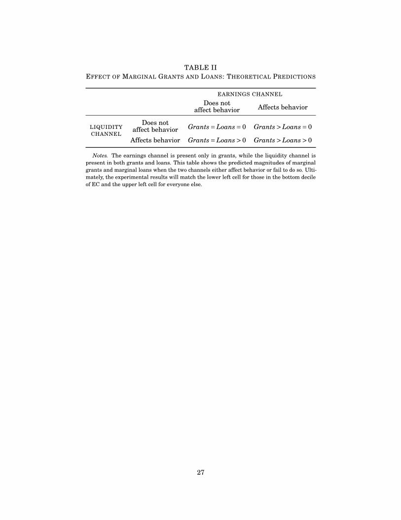


![I j h ] j Z f f Z [ g h c b k p b i e b g u « J h k k b c ...€¦ · I j h ] j Z f f Z [ g h c b k p b i e b g u G Z m q g h- b k k e _ ^ h \ Z l _ e v k d b c Z j « J h k k b](https://static.documents.pub/doc/80x56/60179adf752cac2edc51409b/i-j-h-j-z-f-f-z-g-h-c-b-k-p-b-i-e-b-g-u-j-h-k-k-b-c-i-j-h-j-z-f-f-z.jpg)

![N ? > ? J : E V G U = H J G U I J H F U R E ? G G U G ...J h k k b c k d h c N _ ^ _ j Z p b b 20.06.03 ., j _ ] b k l j Z p b h g g № 4782. < \ _ ^ _ g c k l \ b _ I j b d](https://static.documents.pub/doc/80x56/5f01d0087e708231d40128ec/n-j-e-v-g-u-h-j-g-u-i-j-h-f-u-r-e-g-g-u-g-j-h-k-k-b-c-k-d-h-c.jpg)


