Abstract Prior results on input reconstruction for multi-input, multi-output discrete-time linear systems are extended by defining l-delay input and initial-state observ-ability. This property provides the foundation for reconstructing both unknown in-puts and unknown initial conditions, and thus is a stronger notion than l-delay leftinvertibility, which allows input reconstruction only when the initial state is known.These properties are linked by the main result (Theorem 4), which states that a MIMOdiscrete-time linear system with at least as many outputs as inputs is l-delay input andinitial-state observable if and only if it is l-delay left invertible and has no invariantzeros. In addition, we prove that the minimal delay for input and state reconstructionis identical to the minimal delay for left invertibility. When transmission zeros arepresent, we numerically demonstrate l-delay input and state reconstruction to showhow the input-reconstruction error depends on the locations of the zeros. Specifically,minimum-phase zeros give rise to decaying input reconstruction error, nonminimum-phase zeros give rise to growing reconstruction error, and zeros on the unit circle giverise to persistent reconstruction error.
S. KirtikarUniversity of Michigan, Ann Arbor, MI, USAe-mail: [email protected]
H. Palanthandalam-MadapusiDepartment of Mechanical and Aerospace Engineering, Syracuse University, Syracuse, NY, USAe-mail: [email protected]
E. ZattoniUniversity of Bologna, Bologna, Italye-mail: [email protected]
D.S. Bernstein (�)Aerospace Engineering Department, University of Michigan, Ann Arbor, MI, USAe-mail: [email protected]
Input reconstruction, that is, the problem of inferring the inputs to a system fromavailable measurements, impacts numerous applications, ranging from machine toolcontrol to cryptography, filtering, and coding. In particular, when unknown inputsrepresent disturbances or the effects of system uncertainties, estimates can be usedto improve the control system performance. In addition, when unknown inputs repre-sent the effect of actuator failures, estimates can be used to implement fault-tolerantcontrol, and thereby enhance system reliability [6]
The reconstruction of unknown inputs under the assumption that the initial stateof the system is either known or zero is addressed by left inversion, a long-studiedproblem in the systems literature [14, 17, 18, 22, 23]. In particular, necessary andsufficient conditions were obtained in [17, 18, 22, 23] for the existence of a lineartime-invariant dynamical system that, when cascaded with the original system, pro-duces as its output the input to the original system. These conditions are given interms of a rank condition on matrices made up of either the system matrices or thesystem Markov parameters. The issue of internal stability of the resulting cascade sys-tem was addressed in [14], which considers both left inversion and the dual problemof right inversion. The issue of internal stability and the effect of nonminimum-phasezeros on input reconstruction were addressed within the context of right inversionalong with the related notions of noncausal inversion, preview, preaction, and steer-ing along zeros [4, 7, 8, 12, 16, 20, 25]. A unified approach to noncausal right andleft inversion is given in [13].
Although the problem of left inversion has been extensively studied, the morerealistic problem of determining the unknown inputs from measurements when theinitial state is nonzero has received less attention. In the continuous-time case, [1] de-fines the notion of an unknown-state, unknown-input-reconstructible system, which ischaracterized through a necessary and sufficient geometric condition, which implies,in particular, that the system has no invariant zeros. Later, [9] and [3] present inputand state asymptotic reconstructors. In particular, the reconstructor of [3] does notrequire differentiators and ensures convergence up to an arbitrary degree of accuracy.More recently, [24] introduces a modified version of the reconstructor of [3], whichprovides an asymptotic estimate of both a function of the state and the unknown in-put; in fact, in [3] it is observed that, in general, the entire state is not needed toreconstruct the unknown inputs.
For discrete-time, minimum-phase systems, [5] introduces a constructive algo-rithm for establishing whether the system is finite-time observable and left invertiblewith or without sampling delays, and provides a procedure for obtaining an estimatorthat allows both the unknown input and state to be retrieved after a finite number ofsampling intervals.
The input-reconstruction problem is distinct from, but closely related to, the prob-lem of state observation with unknown inputs. In both problems, the inputs are un-
Circuits Syst Signal Process (2011) 30: 233–262 235
known. However, unlike the input-reconstruction problem, the problem of state ob-servation with unknown inputs does not seek estimates of the unknown inputs. Theliterature on unknown-input observers is extensive; see, for example, [19, 21].
In this paper we extend the results of [15] on one-step-delay exact input recon-struction in discrete-time systems by deriving a reconstructor for l-step-delay inputand initial-state reconstruction, where the delay l accounts for the relative degreeof the system. This reconstructor uses an input-output model that depends on theobservability matrix and a block-Toeplitz matrix of Markov parameters. The mainresult, given by Theorem 4, states that a MIMO discrete-time linear system with atleast as many outputs as inputs is l-delay input and initial-state observable if andonly if it is l-delay left invertible and has no invariant zeros. A computational proce-dure is given by Proposition 7. In addition, we prove that the minimal delay for inputand state reconstruction is identical to the minimal delay for left inversion. Wheninvariant zeros are present, we demonstrate l-delay input and initial-state reconstruc-tion on several numerical examples to show how the input-reconstruction error de-pends on the locations of the zeros. Specifically, minimum-phase zeros give rise todecaying input-reconstruction error, nonminimum-phase zeros give rise to growinginput-reconstruction error, and zeros on the unit circle give rise to persistent input-reconstruction error.
We apply the l-step-delay reconstructor to several numerical examples to showhow the input-reconstruction error depends on the locations of the zeros. Specifically,we show that minimum-phase zeros give rise to decaying input-reconstruction error,nonminimum-phase zeros give rise to growing reconstruction error, and zeros on theunit circle give rise to persistent reconstruction error. The effect of nonminimum-phase zeros shows that this feature increases the delay needed to obtain accurateestimates of the unknown inputs.
In Sect. 2, we state the objective of the paper and introduce notation. In Sect. 3,we review necessary and sufficient conditions for l-delay left invertibility. These re-sults unify and extend standard conditions for left invertibility, and thus provide thefoundation for subsequent results on input reconstruction. In Sect. 4, we focus on theproblem of input reconstruction with l-step delay when the initial conditions of thesystem are nonzero and unknown. The basic notion of l-delay input and initial-stateobservability is defined and characterized through necessary and sufficient algebraicconditions. Sections 5 and 6 illustrate the effect of invariant zeros on the solvability ofthe input and initial-state reconstruction problem. Several numerical examples helpto clarify the new notions and illustrate the effectiveness of the proposed methods.
A preliminary version of some of the results in this paper appeared in the confer-ence paper [10].
2 Problem Statement
Consider the linear discrete-time system
xk+1 = Axk + Buk, (1)
yk = Cxk + Duk, (2)
236 Circuits Syst Signal Process (2011) 30: 233–262
where k is a nonnegative integer, uk ∈ Rm, xk ∈ R
n, yk ∈ Rp , A ∈ R
n×n, B ∈ Rn×m,
C ∈ Rp×n, and D ∈ R
p×m. We assume that (A,B,C,D) is minimal. The p × m
transfer function of (1), (2) is G(z) = C(zIn − A)−1B + D. For each nonnegativeinteger r , we define the output sequence Y[k:k+r] ∈ R
p(r+1) and the input sequenceU[k:k+r] ∈ R
m(r+1) by
Y[k:k+r]�=
⎡⎢⎢⎣
yk
yk+1...
yk+r
⎤⎥⎥⎦ , U[k:k+r]
�=
⎡⎢⎢⎣
uk
uk+1...
uk+r
⎤⎥⎥⎦ . (3)
The objective is to use measurements of the output vector Y[0:r1] to determine theinitial state x0 and the input vector U[0:r2], where r1 ≥ r2 ≥ 0. The goal is to determinevalues of r1 and r2 for which input reconstruction is possible.
Note that Y[0:r], U[0:r], and x0 are related by
Y[0:r] = Γrx0 + Mr,rU[0:r] = Ψr,r
[x0
U[0:r]
], (4)
where, for r1 ≥ r2 ≥ 0, Γr1 ∈ Rp(r1+1)×n, Mr1,r2 ∈ R
p(r1+1)×m(r2+1), and Ψr1,r2 ∈R
p(r1+1)×[n+m(r2+1)] are defined by
Γr1
�=
⎡⎢⎢⎢⎢⎣
C
CA
CA2
...
CAr1
⎤⎥⎥⎥⎥⎦
, Mr1,r2
�=
⎡⎢⎢⎢⎢⎢⎢⎢⎢⎢⎣
H0 0 . . . 0
H1 H0. . .
...
H2 H1. . . 0
......
. . . H0...
......
...
Hr1 Hr1−1 . . . Hr1−r2
⎤⎥⎥⎥⎥⎥⎥⎥⎥⎥⎦
, (5)
and
Ψr1,r2
�= [Γr1 Mr1,r2
], (6)
and where
Hk�={
D, k = 0,
CAk−1B, k ≥ 1,(7)
denote the Markov parameters of the system. Note that Mr,0 ∈ Rp(r+1)×m. Further-
more, for all z ∈ C such that |z| > ρ(A), where ρ(A) denotes the spectral radius of A,it follows that
G(z) =∞∑i=0
z−iHi. (8)
Throughout this paper, d denotes the relative degree of G(z), that is, the smallestnonnegative integer i such that Hi �= 0.
Circuits Syst Signal Process (2011) 30: 233–262 237
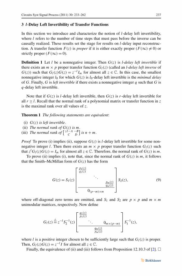
3 l-Delay Left Invertibility of Transfer Functions
In this section we introduce and characterize the notion of l-delay left invertibility,where l refers to the number of time steps that must pass before the inverse can becausally realized. These results set the stage for results on l-delay input reconstruc-tion. A transfer function F(z) is proper if it is either exactly proper (F(∞) �= 0) orstrictly proper (F(∞) = 0).
Definition 1 Let l be a nonnegative integer. Then G(z) is l-delay left invertible ifthere exists an m × p proper transfer function Gl(z) (called an l-delay left inverse ofG(z)) such that Gl(z)G(z) = z−lIm for almost all z ∈ C. In this case, the smallestnonnegative integer l0 for which G(z) is l0-delay left invertible is the minimal delayof G. Finally, G is left invertible if there exists a nonnegative integer q such that G isq-delay left invertible.
Note that if G(z) is l-delay left invertible, then G(z) is r-delay left invertible forall r ≥ l. Recall that the normal rank of a polynomial matrix or transfer function in z
is the maximal rank over all values of z.
Theorem 1 The following statements are equivalent:
(i) G(z) is left invertible.(ii) The normal rank of G(z) is m.
(iii) The normal rank of[
zI−A −BC D
]is n + m.
Proof To prove (i) implies (ii), suppose G(z) is l-delay left invertible for some non-negative integer l. Then there exists an m × p proper transfer function Gl(z) suchthat zlGl(z)G(z) = Im for almost all z ∈ C. Therefore, the normal rank of G(z) is m.
To prove (ii) implies (i), note that, since the normal rank of G(z) is m, it followsthat the Smith–McMillan form of G(z) has the form
G(z) = S1(z)
⎡⎢⎢⎢⎢⎣
p1(z)q1(z)
. . .pm(z)qm(z)
0(p−m)×m
⎤⎥⎥⎥⎥⎦
S2(z), (9)
where off-diagonal zero terms are omitted, and S1 and S2 are p × p and m × m
unimodular matrices, respectively. Now define
Gl(z)�= z−lS−1
2 (z)
⎡⎢⎢⎣
q1(z)p1(z)
. . . 0m×(p−m)
qm(z)pm(z)
⎤⎥⎥⎦S−1
1 (z),
where l is a positive integer chosen to be sufficiently large such that Gl(z) is proper.Then, Gl(z)G(z) = z−lI for almost all z ∈ C.
Finally, the equivalence of (ii) and (iii) follows from Proposition 12.10.3 of [2]. �
238 Circuits Syst Signal Process (2011) 30: 233–262
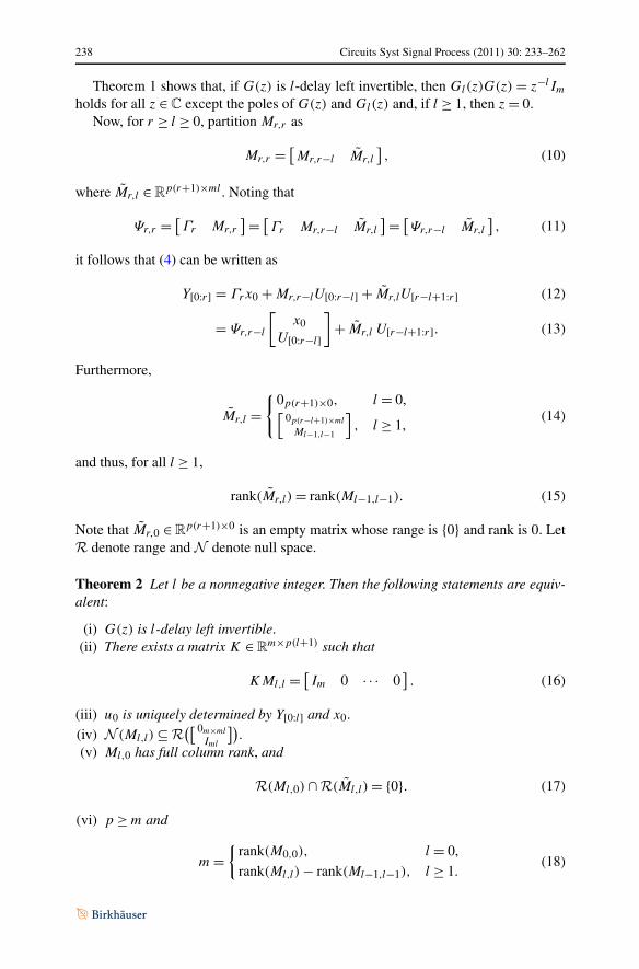
Theorem 1 shows that, if G(z) is l-delay left invertible, then Gl(z)G(z) = z−lIm
holds for all z ∈ C except the poles of G(z) and Gl(z) and, if l ≥ 1, then z = 0.Now, for r ≥ l ≥ 0, partition Mr,r as
Note that Mr,0 ∈ Rp(r+1)×0 is an empty matrix whose range is {0} and rank is 0. Let
R denote range and N denote null space.
Theorem 2 Let l be a nonnegative integer. Then the following statements are equiv-alent:
(i) G(z) is l-delay left invertible.(ii) There exists a matrix K ∈ R
m×p(l+1) such that
KMl,l = [Im 0 · · · 0]. (16)
(iii) u0 is uniquely determined by Y[0:l] and x0.(iv) N (Ml,l) ⊆ R
([ 0m×ml
Iml
]).
(v) Ml,0 has full column rank, and
R(Ml,0) ∩ R(Ml,l) = {0}. (17)
(vi) p ≥ m and
m ={
rank(M0,0), l = 0,
rank(Ml,l) − rank(Ml−1,l−1), l ≥ 1.(18)
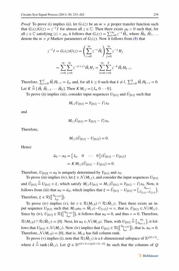
Circuits Syst Signal Process (2011) 30: 233–262 239
Proof To prove (i) implies (ii), let Gl(z) be an m × p proper transfer function suchthat Gl(z)G(z) = z−lI for almost all z ∈ C. Then there exists ρ0 > 0 such that, forall z ∈ C satisfying |z| > ρ0, it follows that Gl(z) =∑∞
i=0 z−i Hi , where H0, H1, . . .
denote the m × p Markov parameters of Gl(z). Now it follows from (8) that
z−lI = Gl(z)G(z) =( ∞∑
i=0
z−i Hi
) ∞∑j=0
z−jHj
=∞∑i=0
∞∑j=0
z−(i+j)HiHj =∞∑
k=0
k∑i=0
z−kHiHk−i .
Therefore,∑l
i=0 HiHl−i = Im and, for all k ≥ 0 such that k �= l,∑k
i=0 HiHk−i = 0.
Let K�= [ Hl Hl−1 · · · H0 ]. Then KMl,l = [Im 0 · · · 0 ].
To prove (ii) implies (iii), consider input sequences U[0:l] and U[0:l] such that
Ml,lU[0:l] = Y[0:l] − Γlx0
and
Ml,lU[0:l] = Y[0:l] − Γlx0.
Therefore,
Ml,l(U[0:l] − U[0:l]) = 0.
Hence
u0 − u0 = [Im 0 · · · 0](U[0:l] − U[0:l])
= KMl,l(U[0:l] − U[0:l]) = 0.
Therefore, U[0:0] = u0 is uniquely determined by Y[0:l] and x0.To prove (iii) implies (iv), let ξ ∈ N (Ml,l), and consider the input sequences U[0:l]
and U[0:l]�= U[0:l] + ξ , which satisfy Ml,lU[0:l] = Ml,lU[0:l] = Y[0:l] − Γlx0. Now, it
follows from (iii) that u0 = u0, which implies that ξ = U[0:l] − U[0:l] = [ 0m×1
U[1:l]−U[1:l]].
Therefore, ξ ∈ R([ 0m×ml
Iml
]).
To prove (iv) implies (v), let ν ∈ R(Ml,0) ∩ R(Ml,l). Then there exists an in-put sequence U[0:l] such that Ml,0u0 = Ml,l(−U[1:l]) = ν, that is, U[0:l] ∈ N (Ml,l).Since by (iv), U[0:l] ∈ R
([ 0m×ml
Iml
]), it follows that u0 = 0, and thus ν = 0. Therefore,
R(Ml,0)∩ R(Ml,l) = {0}. Next, let u0 ∈ N (Ml,0). Then, with U[0:l]�= [ u0
0ml×1
], it fol-
lows that U[0:l] ∈ N (Ml,l). Now (iv) implies that U[0:l] ∈ R([ 0m×ml
Iml
]), that is, u0 = 0.
Therefore, N (Ml,0) = {0}, that is, Ml,0 has full column rank.To prove (v) implies (i), note that R(Ml,l) is a k-dimensional subspace of R
p(l+1),
where k�= rank (Ml,l). Let Q ∈ R
p(l+1)×[p(l+1)−k] be such that the columns of Q
240 Circuits Syst Signal Process (2011) 30: 233–262
form an orthonormal basis of R(Ml,l)⊥. Then
QTMl,l = 0. (19)
Since Ml,0 has full column rank and R(Ml,0)∩ R(Ml,l) = {0}, it follows that QTMl,0has full column rank. Then the generalized inverse (QTMl,0)
† = (MTl,0QQTMl,0)
−1 ×MT
l,0Q satisfies
(QTMl,0
)†QTMl,0 = Im. (20)
Now, it follows from (12), (19), and (20) that
(QTMl,0
)†QT[Y[0:l] − Γlx0] = (QTMl,0
)†QT[Ml,0u0 + Ml,lU[1:l]]
= (QTMl,0)†
QTMl,0u0 = u0.
Now, partition (QTMl,0)†QT as
(QTMl,0
)†QT = [ Kl Kl−1 · · · K0 ] ,
where Ki ∈ Rm×p , i = 0,1, . . . , l. Then it follows from (20) that
∑li=0 KiHl−i =
Im. Next it follows from (19) that (QTMl,0)†QTMl,l = 0, that is, for all k such that
1 ≤ k < l,∑k
i=0 KiHk−i = 0. Now, let Ki = 0 for all i > l, and define Gl(z)�=∑∞
i=0 z−i Ki . Then
Gl(z)G(z) =( ∞∑
i=0
z−i Ki
) ∞∑j=0
z−jHj =∞∑i=0
∞∑j=0
z−(i+j)KiHj
=∞∑
k=0
k∑i=0
z−kKiHk−i = z−ll∑
i=0
KiHl−i = z−lIm.
Hence, Gl(z) is an l-delay left inverse of G(z).To prove that (v) implies (vi), note that rank (Ml,0) = m. For l = 0, it follows that
rank (M0,0) = m. Hence, (vi) holds for l = 0. Next, for l > 0, it follows from (15) and(17) that
rank(Ml,l) = rank[Ml,0 Ml,l
]= rank(Ml,l) + m
= rank(Ml−1,l−1) + m.
To prove (vi) implies (v), suppose l = 0. Then it follows from (18) that M0,0 hasfull column rank. Since M0,0 is an empty matrix, R(M0,0) ∩ R(M0,0) = {0}. Hence,(17) holds for l = 0. Next, for l ≥ 1 note that, since rank (Ml,l) ≤ rank (Ml,l) +rank (Ml,0), it follows from (15) that
rank(Ml,l) ≤ rank(Ml−1,l−1) + rank(Ml,0). (21)
Circuits Syst Signal Process (2011) 30: 233–262 241
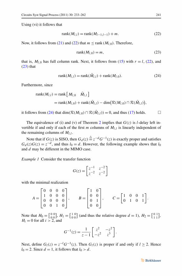
Using (vi) it follows that
rank(Ml,l) = rank(Ml−1,l−1) + m. (22)
Now, it follows from (21) and (22) that m ≤ rank (Ml,0). Therefore,
rank(Ml,0) = m, (23)
that is, Ml,0 has full column rank. Next, it follows from (15) with r = l, (22), and(23) that
rank(Ml,l) = rank(Ml,l) + rank(Ml,0). (24)
Furthermore, since
rank(Ml,l) = rank[Ml,0 Ml,l
]
= rank(Ml,0) + rank(Ml,l) − dim(
R(Ml,0) ∩ R(Ml,l)),
it follows from (24) that dim(R(Ml,0) ∩ R(Ml,l)) = 0, and thus (17) holds. �
The equivalence of (i) and (v) of Theorem 2 implies that G(z) is l-delay left in-vertible if and only if each of the first m columns of Ml,l is linearly independent ofthe remaining columns of Ml,l .
Note that if G(z) is SISO, then Gd(z)�= z−dG−1(z) is exactly proper and satisfies
Gd(z)G(z) = z−d , and thus l0 = d . However, the following example shows that l0and d may be different in the MIMO case.
Example 1 Consider the transfer function
G(z) =[z−1 z−2
z−2 z−2
]
with the minimal realization
A =
⎡⎢⎢⎣
0 0 0 01 0 0 00 0 0 00 0 1 0
⎤⎥⎥⎦ , B =
⎡⎢⎢⎣
1 00 00 10 0
⎤⎥⎥⎦ , C =
[1 0 0 10 1 0 1
].
Note that H0 = [ 0 00 0
], H1 = [ 1 0
0 0
](and thus the relative degree d = 1), H2 = [ 0 1
1 1
],
Hi = 0 for all i > 2, and
G−1(z) = 1
z − 1
[z2 −z2
−z2 z3
].
Next, define Gl(z) = z−lG−1(z). Then Gl(z) is proper if and only if l ≥ 2. Hencel0 = 2. Since d = 1, it follows that l0 > d .
242 Circuits Syst Signal Process (2011) 30: 233–262
The following result gives a necessary and sufficient condition for l0 = d .
Proposition 1 Let l0 denote the minimal delay of G(z), and let l ≥ l0. Then,
rank[H0 · · · Hl
]≥ m, (25)
rank
⎡⎢⎢⎢⎣
H0H1...
Hl
⎤⎥⎥⎥⎦= m, (26)
and l0 ≤ n. Furthermore, l0 ≥ d with equality if and only if rank (Hd) = m.
Proof Suppose l = l0 = 0 so that l0 < n. Then it follows from condition (vi) ofTheorem 2 that rank (M0,0) = rank (H0) = m. Therefore, (25) and (26) hold. Nowsuppose l0 ≥ 0 and l ≥ 1. Then it follows from condition (vi) of Theorem 2 thatrank (Ml,l) − rank (Ml−1,l−1) = m. Since
Ml,l =[
Ml−1,l−1 0Hl · · · H1 H0
], (27)
it follows that rank (Ml−1,l−1) + rank [H0 · · · Hl ] ≥ rank (Ml,l), which implies (25).Furthermore, since G(z) is l-delay left invertible, it follows from condition (v) of
Theorem 2 that Ml,0 has full column rank. Since
Ml,0 =
⎡⎢⎢⎢⎣
H0H1...
Hl
⎤⎥⎥⎥⎦ ,
(26) holds.Next let k ≥ 0 and note that
rank(Mk,k) = rank[Mk,0 Mk,k
]
≤ rank(Mk,0) + rank(Mk,k)
≤ m + rank(Mk,k). (28)
It then follows from (14) that
rank(Mk,k) − rank(Mk−1,k−1) ≤ m. (29)
Since G(z) is l-delay left invertible, it follows from condition (vi) of Theorem 2 that
(29) holds with equality if and only if k ≥ l. Next, define q�= dim(N (D)), and note
that
rank(M0,0) = rank(D) = m − q. (30)
Circuits Syst Signal Process (2011) 30: 233–262 243
Suppose q = 0. Then rank (M0,0) = m, and it follows from (vi) of Theorem 2 thatl0 = 0 and thus l0 ≤ n. Now suppose q ≥ 1. Then it follows from (28) with k = l0that
rank(Ml0,l0) ≤ l0(m − 1) + (m − q) + 1. (31)
Next, define Q�= [Al0B · · · B ]. Since G(z) is left invertible, it follows from (31) that
0 = dim
(N([
Q
Ml0,l0
]))≥ (l0 + q − 1) − n. (32)
Since q ≥ 1 it follows that l0 ≤ n − q + 1 ≤ n.Since Hi = 0 for all i < d , it follows from (25) that l0 ≥ d . Now suppose
l0 = d . Then (25) implies that m ≤ rank [H0 · · ·Hd ] = rank (Hd) ≤ m, and thusrank (Hd) = m. Conversely, suppose rank (Hd) = m. Then Md,0 has full column rankand Md,d = 0. Therefore, condition (v) of Theorem 2 holds with l = d , that is, l0 ≤ d .Since l0 ≥ d , it follows that l0 = d . �
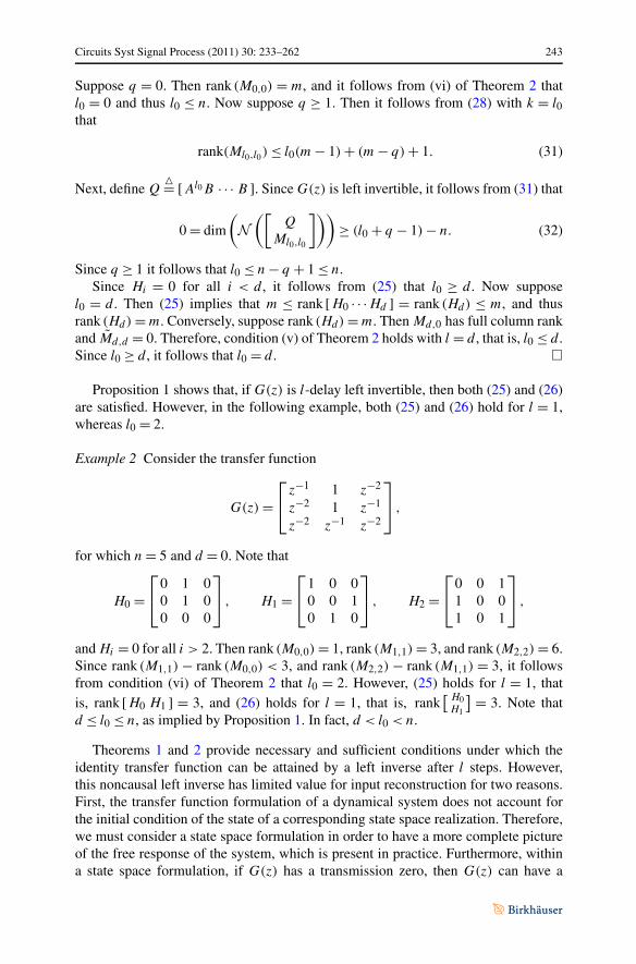
Proposition 1 shows that, if G(z) is l-delay left invertible, then both (25) and (26)are satisfied. However, in the following example, both (25) and (26) hold for l = 1,whereas l0 = 2.
Example 2 Consider the transfer function
G(z) =⎡⎣
z−1 1 z−2
z−2 1 z−1
z−2 z−1 z−2
⎤⎦ ,
for which n = 5 and d = 0. Note that
H0 =⎡⎣
0 1 00 1 00 0 0
⎤⎦ , H1 =
⎡⎣
1 0 00 0 10 1 0
⎤⎦ , H2 =
⎡⎣
0 0 11 0 01 0 1
⎤⎦ ,
and Hi = 0 for all i > 2. Then rank (M0,0) = 1, rank (M1,1) = 3, and rank (M2,2) = 6.Since rank (M1,1) − rank (M0,0) < 3, and rank (M2,2) − rank (M1,1) = 3, it followsfrom condition (vi) of Theorem 2 that l0 = 2. However, (25) holds for l = 1, thatis, rank [H0 H1 ] = 3, and (26) holds for l = 1, that is, rank
[ H0H1
] = 3. Note thatd ≤ l0 ≤ n, as implied by Proposition 1. In fact, d < l0 < n.
Theorems 1 and 2 provide necessary and sufficient conditions under which theidentity transfer function can be attained by a left inverse after l steps. However,this noncausal left inverse has limited value for input reconstruction for two reasons.First, the transfer function formulation of a dynamical system does not account forthe initial condition of the state of a corresponding state space realization. Therefore,we must consider a state space formulation in order to have a more complete pictureof the free response of the system, which is present in practice. Furthermore, withina state space formulation, if G(z) has a transmission zero, then G(z) can have a
244 Circuits Syst Signal Process (2011) 30: 233–262
nonzero input such that, for some nonzero initial condition of a corresponding statespace model, the output is identically zero. We explore these issues in the followingsections.
4 l-Delay Input Reconstruction with Known Initial State
In this section we show that if G(z) is l-delay left invertible then we can achieveinput reconstruction with an l-step delay from a known initial condition x0 and outputmeasurements Y[0:r].
Lemma 1 Assume that G(z) is l-delay left invertible. Then, for all r ≥ l,
N (Mr,r ) ⊆ R([
0m(r−l+1)×ml
Iml
]). (33)
Proof Note that
Ml+1,l+1 =[Ml+1,0
0p×m(l+1)
Ml,l
]=[
Ml,0 Ml,l 0p(l+1)×m
Hl+1 Hl · · · H1 H0
]. (34)
Since G(z) is l-delay left invertible it follows from condition (v) of Theorem 2that Ml,0 has full column rank. Then it follows from (34) that Ml+1,0 has full col-umn rank. Since R(Ml,0) ∩ R(Ml,l) = {0} and Ml,0 has full column rank, it follows
from (34) that R(Ml+1,0) ∩ R([ 0p×m(l+1)
Ml,l
])= {0}. Then Ml+1,1 = [Ml+1,0∣∣ 0p×m
Ml,0
]has
full column rank and R(Ml+1,1) ∩ R(Ml+1,l) = {0}. Let ξ1 ∈ C2m and ξ2 ∈ C
ml besuch that Ml+1,1ξ1 + Ml+1,lξ2 = 0, that is
[ ξ1ξ2
] ∈ N (Ml+1,l+1). Since R(Ml+1,1) ∩R(Ml+1,l) = {0}, it follows that Ml+1,1ξ1 = 0. Since Ml+1,1 has full column rank,it follows that ξ1 = 0. Therefore, N (Ml+1,l+1) ⊆ R
([ 02m×ml
Iml
]). Hence, (33) holds
with r = l + 1. Proceeding similarly, we attain N (Mr,r ) ⊆ R([ 0m(r−l+1)×ml
Iml
])for all
r ≥ l. �
Theorem 3 Assume that G(z) is l-delay left invertible. Then, for all r ≥ l, U[0:r−l]is uniquely determined by x0 and Y[0:r]. Furthermore, the unique solution of (4) withreconstruction delay l is
U[0:r−l] = row[1:(r−l+1)m][M†
r,r (Y[0:r] − Γrx0)]. (35)
Proof Note that (4) implies
Mr,rU[0:r] = Y[0:r] − Γrx0. (36)
Then it follows from Proposition 6.1.7(v) of [2] that
U[0:r] = M†r,r (Y[0:r] − Γrx0) + (I − M†
r,rMr,r )U[0:r]. (37)
Circuits Syst Signal Process (2011) 30: 233–262 245
Using Proposition 6.1.6(viii) of [2] it follows that R(I − M†r,rMr,r ) = N (Mr,r ).
In this section we take into account the unknown and possibly nonzero initial condi-tion of (1), (2) and consider the problem of input and initial-state reconstruction. Thefollowing definition provides the foundation for input and initial-state reconstruction.For the following definition, recall the definition of Ψr1,r2 given by (6).
Definition 2 Let l be a nonnegative integer. The system (1), (2) is l-delay input andinitial-state observable (IISO) if there exists r ≥ l such that
N (Ψr,r ) ⊆ R([
0[n+m(r−l+1)]×lm
Ilm
]). (38)
In this case, the smallest nonnegative integer l′0 for which (1), (2) is l′0-delay inputand initial-state observable is the minimal IISO delay. Furthermore, (1), (2) is inputand initial-state observable if there exists a nonnegative integer q such that (1), (2)is q-delay input and initial-state observable.
In Definition 2, r + 1 is the length of the output data window used to reconstructthe input and initial state. Specifically, if Y[0:r] = 0 in (4), that is,
[x0
U[0:r]
]=⎡⎣
x0U[0:r−l]
U[r−l+1:r]
⎤⎦ ∈ N (Ψr,r ),
then (38) implies that[ x0
U[0:r−l]]= 0, and thus x0 and U[0:r−l] can be uniquely recon-
structed from Y[0:r].The following result provides necessary and sufficient conditions for l-delay input
and initial-state observability.
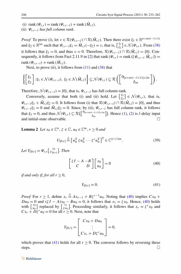
Proposition 2 Let l be a nonnegative integer. The system (1), (2) is l-delay input andinitial-state observable if and only if there exists r ≥ l such that both of the followingstatements hold:
246 Circuits Syst Signal Process (2011) 30: 233–262
(i) rank (Ψr,r ) = rank (Ψr,r−l) + rank (Mr,l).(ii) Ψr,r−l has full column rank.
Proof To prove (i), let ν ∈ R(Ψr,r−l) ∩ R(Mr,l). Then there exist ξ1 ∈ Rn+m(r−l+1)
and ξ2 ∈ Rlm such that Ψr,r−lξ1 = Mr,l(−ξ2) = ν, that is,
[ ξ1ξ2
] ∈ N (Ψr,r ). From (38)
it follows that ξ1 = 0, and thus ν = 0. Therefore, R(Ψr,r−l) ∩ R(Mr,l) = {0}. Con-sequently, it follows from Fact 2.11.9 in [2] that rank (Ψr,r ) = rank ([Ψr,r−l Mr,l ]) =rank (Ψr,r−l ) + rank (Mr,l).
Next, to prove (ii), it follows from (11) and (38) that
{[ξ1ξ2
]: ξ1 ∈ N (Ψr,r−l), ξ2 ∈ N (Mr,l)
}⊆ N (Ψr,r ) ⊆ R
([0[n+m(r−l+1)]×lm
Ilm
]).
Therefore, N (Ψr,r−l) = {0}, that is, Ψr,r−l has full column rank.Conversely, assume that both (i) and (ii) hold. Let
[ ξ1ξ2
] ∈ N (Ψr,r ), that is,
Ψr,r−lξ1 + Mr,lξ2 = 0. It follows from (i) that R(Ψr,r−l ) ∩ R(Mr,l) = {0}, and thusΨr,r−lξ1 = 0 and Mr,lξ2 = 0. Since, by (ii), Ψr,r−l has full column rank, it follows
that ξ1 = 0, and thus N (Ψr,r ) ⊆ R([ 0[n+m(r−l+1)]×lm
Ilm
]). Hence (1), (2) is l-delay input
and initial-state observable. �
Lemma 2 Let x0 ∈ Cn, ζ ∈ C, u0 ∈ C
m, r ≥ 0 and
U[0:r]�= [uT
0 ζuT0 · · · ζ ruT
0
]T ∈ C(r+1)m. (39)
Let Y[0:r] = Ψr,r
[ x0U[0:r]
]. Then
[ζ I − A −B
C D
][x0u0
]= 0 (40)
if and only if, for all r ≥ 0,
Y[0:r] = 0. (41)
Proof For r ≥ 1, define xr�= Axr−1 + Bζ r−1u0. Noting that (40) implies Cx0 +
Du0 = 0 and (ζ I − A)x0 − Bu0 = 0, it follows that x1 = ζx0. Hence, (40) holdswith
[ x0u0
]replaced by
[ x1ζu0
]. Proceeding similarly, it follows that xr = ζ rx0 and
Cxr + Dζru0 = 0 for all r ≥ 0. Next, note that
Y[0:r] =⎡⎢⎣
Cx0 + Du0...
Cxr + Dζru0
⎤⎥⎦= 0,
which proves that (41) holds for all r ≥ 0. The converse follows by reversing thesesteps. �
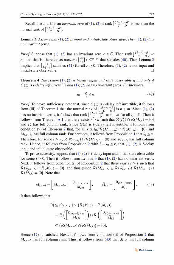
Circuits Syst Signal Process (2011) 30: 233–262 247
Recall that ζ ∈ C is an invariant zero of (1), (2) if rank[
ζ I−A −B
C D
]is less than the
normal rank of[
zI−A −BC D
].
Lemma 3 Assume that (1), (2) is input and initial-state observable. Then (1), (2) hasno invariant zeros.
Proof Suppose that (1), (2) has an invariant zero ζ ∈ C. Then rank[
ζ I−A −B
C D
]<
n + m, that is, there exists nonzero[ x0
u0
] ∈ Cn+m that satisfies (40). Then Lemma 2
implies that[ x0
U[0:r]]
satisfies (41) for all r ≥ 0. Therefore, (1), (2) is not input andinitial-state observable. �
Theorem 4 The system (1), (2) is l-delay input and state observable if and only ifG(z) is l-delay left invertible and (1), (2) has no invariant zeros. Furthermore,
l0 = l′0 ≤ n. (42)
Proof To prove sufficiency, note that, since G(z) is l-delay left invertible, it followsfrom (iii) of Theorem 1 that the normal rank of
[zI−A −B
C D
]is n + m. Since (1), (2)
has no invariant zeros, it follows that rank[
ζ I−A −B
C D
]= n + m for all ζ ∈ C. Then itfollows from Theorem A.1 that there exists r ≥ n such that R(Γr) ∩ R(Mr,r ) = {0}and Γr has full column rank. Since G(z) is l-delay left invertible, it follows fromcondition (v) of Theorem 2 that, for all r ≥ l0, R(Mr,r−l0) ∩ R(Mr,l0) = {0} andMr,r−l0 has full column rank. Furthermore, it follows from Proposition 1 that l0 ≤ n.Therefore, for some r ≥ n, R(Ψr,r−l0) ∩ R(Mr,l0) = {0} and Ψr,r−l0 has full columnrank. Hence, it follows from Proposition 2 with l = l0 ≤ r , that (1), (2) is l-delayinput and initial-state observable.
To prove necessity, suppose that (1), (2) is l-delay input and initial-state observablefor some l ≥ 0. Then it follows from Lemma 3 that (1), (2) has no invariant zeros.Next, it follows from condition (i) of Proposition 2 that there exists r ≥ l such thatR(Ψr,r−l ) ∩ R(Mr,l) = {0}, and thus (since R(Mr,r−l) ⊆ R(Ψr,r−l)) R(Mr,r−l ) ∩R(Mr,l) = {0}. Note that
Mr,r−l =[Mr,r−l−1
0p(r−l)×m
Ml,0
], Mr,l =
[0p(r−l)×ml
Ml,l
]. (43)
It then follows that
{0} ⊆ {0p(r−l)} × (R(Ml,0) ∩ R(Ml,l))
= R([
0p(r−l)×m
Ml,0
])∩ R
([0p(r−l)×ml
Ml,l
])
⊆ (R(Mr,r−l ) ∩ R(Mr,l))= {0}.
Hence (17) is satisfied. Next, it follows from condition (ii) of Proposition 2 thatMr,r−l has full column rank. Thus, it follows from (43) that Ml,0 has full column
248 Circuits Syst Signal Process (2011) 30: 233–262
rank. It then follows from condition (v) of Theorem 2 that G(z) is l-delay left invert-ible.
Finally, it follows from Proposition 1 and the arguments used in the previous para-graphs that l0 = l′0 ≤ n. �
Let def(M) denote the defect of the matrix M , that is, the dimension of the nullspace of M .
Proposition 3 Assume that G(z) is SISO and (1), (2) is input and initial-state ob-servable. Then
l0 = l′0 = d = n. (44)
Furthermore, for all r ≥ n − 1, def(Ψr,r ) = n.
Proof Let l ≥ 0 be such that (1), (2) is l-delay input and state observable. Then itfollows from Theorem 4 that G(z) is l-delay left invertible and has no invariant zeros.Since G(z) is SISO it follows that z−dG−1(z) is exactly proper, and thus l ≥ l0 = d .Since G(z) has no zeros it follows that n = d . It then follows from Theorem 4 thatl0 = l′0 = d = n.
Finally, let r ≥ n. Then Ψr,r = [Γr
∣∣Mr,r−n
∣∣ 0(r+1−n)×n
Mn,n
]. Since Hn �= 0 it follows
that Mr,r−n has full column rank and thus Ψr,r−n = [Γr Mr,r−n ] has full columnrank. Since Mn,n = 0 it follows that
def(Ψr,r ) = dim(
N (Ψr,r ))= rank
[0(r+1−n)×n
In
]= n. �
Proposition 4 Let m = 1 and assume that (1), (2) is input and initial-state observ-able. Then
l0 = l′0 = d ≤ n. (45)
Proof Let l ≥ 0 be such that (1), (2) is l-delay input and state observable. Then itfollows from Theorem 4 that G(z) is l-delay left invertible and (1), (2) has no in-variant zeros. Since G(z) is SIMO it follows that Hd has full column rank. Then itfollows from Proposition 1 that l0 = d . Therefore, it follows from Theorem 4 thatl0 = l′0 = d ≤ n. �
The following SIMO example is input and initial-state observable and satisfiesd < n.
Example 3 Consider the transfer function
G(z) =[ 1
z
1z2
],
Circuits Syst Signal Process (2011) 30: 233–262 249
with the minimal realization
A =[
0 10 0
], B =
[01
], C =
[0 11 0
], D =
[00
].
Then H1 = [ 10
]has full column rank and d = 1. It then follows from Proposition 1
that G(z) is 1-delay left invertible and l0 = 1. Next it follows from Proposition 4 thatl0 = l′0 = d ≤ n = 2. In fact, d < n.
Proposition 5 Assume that (1), (2) is input and initial-state observable. Then
d ≤ l0 = l′0 ≤ n. (46)
Proof Since (1), (2) is input and initial-state observable, it follows from Theorem 4that l0 = l′0 ≤ n and G(z) is l0-delay left invertible. It then follows from Proposition 1that d ≤ l0. Hence (46) is satisfied. �
The following result provides necessary conditions for l-delay input and initial-state observability.
Proposition 6 Let l be a nonnegative integer, and assume that (1), (2) is l-delay inputand initial-state observable. Then the following statements hold:
(i) (1), (2) is k-delay input and initial-state observable for all k ≥ l.(ii) rank (Ψr,r−l) = rank (Ψr,r−l−1) + m for all r ≥ n.
(iii) m ≤ p.(iv) If m = p, then n ≤ ml.(v) rank (Γn−1) = n.
Proof To prove (i), since (1), (2) is l-delay input and initial-state observable, thereexists r ≥ l such that (38) holds. Now, note that
Ψr+1,r−l =[
Ψr,r−l
CAr+1 Hr+1 · · · Hl+1
](47)
and
Mr+1,l+1 =
⎡⎢⎢⎢⎢⎢⎢⎣
0...
H0...
Hl
0p×ml
Mr,l
⎤⎥⎥⎥⎥⎥⎥⎦
=[
Mr,l 0p(r+1)×m
Hl · · · H1 H0
]. (48)
Then it follows from condition (ii) of Proposition 2 that Ψr,r−l has full column rank.It then follows from (47) that Ψr+1,r−l has full column rank. Next, it follows from
250 Circuits Syst Signal Process (2011) 30: 233–262
condition (i) of Proposition 2 that R(Ψr,r−l ) ∩ R(Mr,l) = {0}. Then it follows from(47)–(48) that R(Ψr+1,r−l) ∩ R(Mr+1,l+1) = {0}. Since
⎡⎢⎢⎢⎢⎢⎢⎣
0...
H0...
Hl
⎤⎥⎥⎥⎥⎥⎥⎦
has full column rank, it follows from (48) that Ψr+1,r+1−l has full column rankand rank (Ψr+1,r+1) = rank (Ψr+1,r+1−l) + rank (Mr+1,l). Hence, N (Ψr+1,r+1) ⊆R([ 0[n+(r−l+2)m)]×lm
Ilm
]). Proceeding similarly, for all s ≥ r ,
N (Ψs,s) ⊆ R([
0[n+(s−l+1)m)]×lm
Ilm
]). (49)
Let s ≥ k ≥ l. Then
R([
0[n+(s−l+1)m)]×lm
Ilm
])⊆ R
([0[n+(s−k+1)m)]×km
Ikm
]),
and it follows from (38) that
N (Ψs,s) ⊆ R([
0[n+(s−k+1)m)]×km
Ikm
]).
Hence, (1), (2) is k-delay input and initial-state observable.Next, to prove (ii), it follows from (ii) of Proposition 2 that
has full column rank and thus Ψr,r−l−1 and the last m columns of Ψr,r−l have fullcolumn rank. Therefore, rank (Ψr,r−l) = rank (Ψr,r−l−1) + m.
Next, to prove (iii), since Proposition 2 holds for all r ≥ n, it follows that Ψr,r−l
has full column rank, that is, n+m(r − l +1) ≤ p(r +1) for all r > l. Hence, m ≤ p.Next, to prove (iv), it follows from (ii) of Proposition 2 that n + m(r − l + 1) ≤
p(r + 1). Now with m = p, it follows that n ≤ ml.Next, to prove (v), it follows from (ii) of Proposition 2 that Ψr,r−l has full column
rank, and thus Γr has full column rank. Therefore, rank (Γn−1) = n. �
The following result provides an explicit reconstructor for the l-delay input andinitial-state reconstruction problem.
Proposition 7 Assume that (1), (2) is l-delay input and initial-state observable and(38) holds for some r ≥ l. Then x0 and U[0:r−l] are uniquely determined by Y[0:r].Furthermore, the unique solution of (12) with reconstruction delay l is given by
[x0
U[0:r−l]
]= (QTΨr,r−l
)†QTY[0:r], (50)
Circuits Syst Signal Process (2011) 30: 233–262 251
where † represents the Moore–Penrose generalized inverse, k�= rank (Mr,l), and the
columns of Q ∈ Rp(r+1)×[p(r+1)−k] are an orthonormal basis of N (MT
r,l).
Proof Let r ≥ l ≥ d , and ξ = [ x0U[0:r−l]
]. By assumption, each row of QT is an element
of R(Mr,l)⊥. Therefore,
QTMr,l = 0. (51)
Since by (ii) of Proposition 2, Ψr,r−l has full column rank, it follows that QTΨr,r−l
has full column rank. Then the generalized inverse (QTΨr,r−l)† = (Ψ T
r,r−lQ ×QTΨr,r−l)
−1Ψ Tr,r−lQ satisfies
(QTΨr,r−l
)†QTΨr,r−l = In+(r−l+1)m. (52)
Now, it follows from (12), (51), and (52) that
(QTΨr,r−l
)†QTY[0:r] = (QTΨl,0
)†QT(Ψr,r−lξ + Mr,lU[r−l+1:r]
)
= (QTΨr,r−l
)†QTΨr,r−lξ = ξ. �
The special case l = 1, d = 1 is given in [15]. Proposition 2 shows that, forthis special case (1), (2) is 1-delay input and initial-state observable if and onlyif there exists r ≥ 1 such that Ψr,r−1 has full column rank. Furthermore, sinceMr,1 = 0(r+1)p×m, it follows from Proposition 5 that Q = I(r+1)p and it follows from(50) that the unique solution of (12) for each r ≥ 1 is given by
[x0
U[0:r−1]
]= Ψ
†r,r−1Y[0:r]. (53)
Example 4 Consider the transfer function
G(z) = 1
(z − 0.5)(z − 0.6),
with the minimal realization
A =[
1.1 −0.60.5 0
], B =
[20
], C = [0 1
], D = [0
].
Since Ψ2,0 has full column rank, Ψ2,1 does not have full column rank, andrank (Ψ2,2) = rank (Ψ2,0) + rank (M2,2), it follows from Proposition 2 that G(z) is2-delay input and initial-state observable but not 1-delay input and initial-state ob-servable. Therefore, l′0 = 2. Since G(z) is SISO with d = 2, it follows that l0 = d
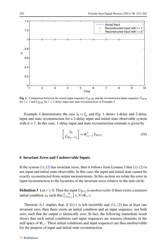
and thus l0 = l′0 = 2. For both cases we compute the least-squares expression in (50),and Fig. 1 compares 1-delay and 2-delay input and state reconstruction. As expected,2-delay input and state reconstruction described by (50) correctly estimates the inputand initial state, whereas, for l = 1, the solution given by (50) fails.
252 Circuits Syst Signal Process (2011) 30: 233–262
Fig. 1 Comparison between the actual input sequence U[0:10] and the reconstructed input sequence U[0:9]for l = 1 and U[0:8] for l = 2 delay input and state reconstruction in Example 4
Example 4 demonstrates the case l0 = l′0, and Fig. 1 shows 1-delay and 2-delayinput and state reconstruction for a 2-delay input and initial-state observable systemwith d = 1. In this case, 1-delay input and state reconstruction estimate is given by
[x0
U[0:r−1]
]= Ψ
†r,r−1Y[0:r]. (54)
6 Invariant Zeros and Unobservable Inputs
If the system (1), (2) has invariant zeros, then it follows from Lemma 3 that (1), (2) isnot input and initial-state observable. In this case, the input and initial state cannot beexactly reconstructed from output measurements. In this section we relate the error ininput reconstruction to the locations of the invariant zeros relative to the unit circle.
Definition 3 Let r ≥ 0. Then the input U[0:r] is unobservable if there exists a nonzeroinitial condition x0 such that
[ x0U[0:r]
] ∈ N (Ψr,r ).
Theorem A.1 implies that, if G(z) is left invertible and (1), (2) has at least oneinvariant zero, then there exists an initial condition and an input sequence, not bothzero, such that the output is identically zero. In fact, the following immediate resultshows that such initial conditions and input sequences are nonzero elements in thenull space of Ψr,r . These initial conditions and input sequences are thus unobservablefor the purpose of input and initial-state reconstruction.
Circuits Syst Signal Process (2011) 30: 233–262 253
Proposition 8 Let ξ ∈ Rn and ν ∈ R
(r+1)m be such that
Ψr,r
[ξ
ν
]= Γrξ + Mr,rν = 0. (55)
Then, with x0 = ξ and U[0:r] = ν, it follows that Y[0:r] = 0.
For SIMO systems that have a zero outside of the spectral radius of A, the follow-ing result provides an explicit expression for an unobservable input and initial state.
Proposition 9 Let m = 1 and let ζ ∈ C be an invariant zero of (1), (2) such that|ζ | > ρ(A). Furthermore, let c ∈ C, define the input sequence
uk = Re(cζ k), k = 0,1, . . . , (56)
and let
x0 = Re
[c
∞∑i=1
ζ−iAi−1B
]. (57)
Then, for all r ≥ 0, Y[0:r] = 0, that is,[
x0U[0:r]
]∈ N (Ψr,r ). (58)
Proof Since G(ζ) = 0, it follows from (8) that
cζ r
(r∑
i=0
ζ−iHi +∞∑
i=r+1
ζ−iHi
)= 0, (59)
that is,
[Hr Hr−1 · · · H0 ]ν[0:r] + CArx0 = 0, (60)
where
ν[0:r]�= Re
⎛⎜⎜⎝c
⎡⎢⎢⎣
1ζ 1
...
ζ r
⎤⎥⎥⎦
⎞⎟⎟⎠ .
Note that
∞∑i=1
ζ−iAi−1B =∞∑i=0
ζ−(i+1)AiB.
Now dividing (59) by ζ yields
cζ r
(r−1∑i=0
ζ−(i+1)Hi +∞∑i=r
ζ−(i+1)Hi
)= 0,
254 Circuits Syst Signal Process (2011) 30: 233–262
that is,
[Hr−1 Hr−2 · · · H0 ]ν[0:r−1] + CAr−1x0 = 0. (61)
Proceeding similarly, it follows from (60), (61) and (8) that
Ψr,r
[x0
ν[0:r]
]= 0.
Now, with U[0:r] = ν[0:r] it follows that there exists x0 such that[ x0
U[0:r]] ∈ N (Ψr,r ). �
Note that, if ζ is a zero of (1), (2), then rank[
ζ I−A −B
C D
]< n+m. Furthermore, the
values of x0 given by (57) satisfy[ζ I − A −B
C D
][x0c
]= 0. (62)
Note that if ζ is an element of the open unit disk, then (56) decays, whereas (56)grows if ζ is outside the unit disk. If however, ζ is on the unit disk, then (56) neithergrows nor decays. The following examples illustrate these properties.
Consider a realization of the type of (1), (2), where A, B are given by
A =⎡⎣
0.1 1.7029 00 0.2 10 0 0.3
⎤⎦ , B =
⎡⎣
002
⎤⎦ , (63)
and where C is chosen to set the locations of the invariant zeros relative to the unitcircle. Note that x0 = [10 5 15 ] is used only for simulation, but knowledge of x0is not assumed to be available for input reconstruction.
Example 5 Consider the transfer function
G(z) = z2 − z + 0.5
(z − 0.1)(z − 0.2)(z − 0.3), (64)
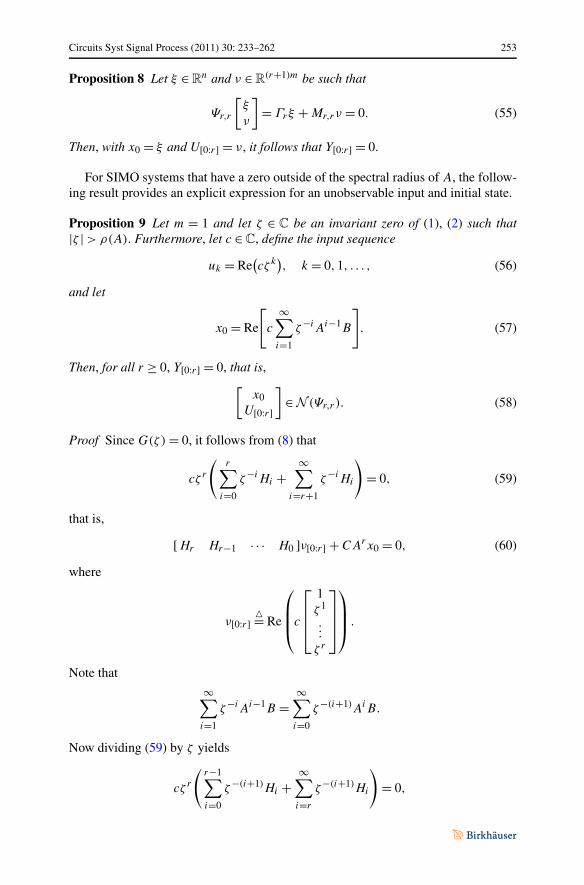
which has minimum-phase zeros 0.5 + 0.5j , 0.5 − 0.5j and C =[0.25 −0.5 2 ]. Figure 2 compares the 1-delay reconstructed input sequence withthe actual input sequence. Note that the input-reconstruction error is largest for smallvalues of k, which corresponds to the fact that the system has minimum-phase zeros.
Example 6 Consider the transfer function
G(z) = z − 1
(z − 0.1)(z − 0.2)(z − 0.3), (65)
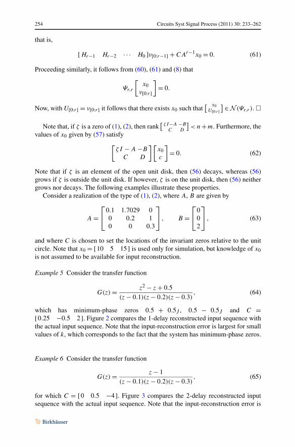
for which C = [0 0.5 −4 ]. Figure 3 compares the 2-delay reconstructed inputsequence with the actual input sequence. Note that the input-reconstruction error is
Circuits Syst Signal Process (2011) 30: 233–262 255
Fig. 2 Comparison between the actual input sequence and the 1-delay reconstructed input of the sys-tem given by Example 5, with minimum-phase zeros 0.5 + 0.5j and 0.5 − 0.5j . In this case, the in-put-reconstruction error is decaying and oscillatory
Fig. 3 Comparison between the actual input sequence and 2-delay reconstructed input of the system givenby Example 6, with zero 1. In this case the input-reconstruction error is persistent; in fact, it is constantover the interval
persistent over the interval, which is a consequence of the fact that the zero is locatedon the unit circle. In addition, the sign of the error is constant due to the fact that thezero is located at 1.
Example 7 Consider the nonminimum-phase transfer function
G(z) = z − 3
(z − 0.1)(z − 0.2)(z − 0.3), (66)
256 Circuits Syst Signal Process (2011) 30: 233–262
Fig. 4 Comparison between the actual input sequence and 1-delay reconstructed input of the system givenby Example 7, with nonminimum-phase zero 3. The input-reconstruction error is monotonically increasingdue to the real nonminimum-phase zero
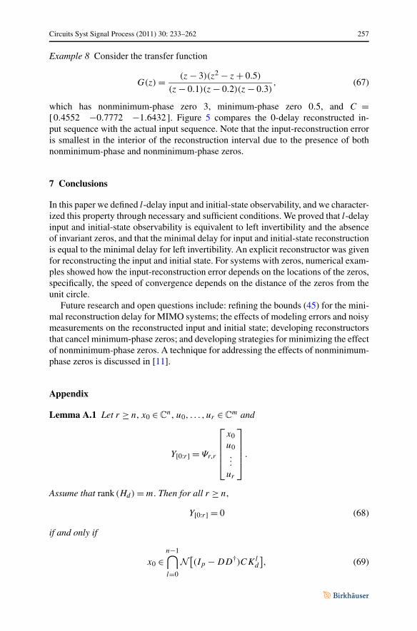
Fig. 5 Comparison between the actual input and the 0-delay reconstructed input for the system given byExample 8, with nonminimum-phase zero 3 and minimum-phase zeros 0.5 + 0.5j and 0.5 − 0.5j . Theinput-reconstruction error is smallest in the interior of the reconstruction interval due to the presence ofboth nonminimum-phase and nonminimum-phase zeros
for which C = [−0.8515 0.5000 0 ]. Figure 4 compares the 1-delay reconstructedinput sequence with the actual input sequence. Note that the input-reconstructionerror is monotonically increasing due to the real nonminimum-phase zero.
Circuits Syst Signal Process (2011) 30: 233–262 257
Example 8 Consider the transfer function
G(z) = (z − 3)(z2 − z + 0.5)
(z − 0.1)(z − 0.2)(z − 0.3), (67)
which has nonminimum-phase zero 3, minimum-phase zero 0.5, and C =[0.4552 −0.7772 −1.6432 ]. Figure 5 compares the 0-delay reconstructed in-put sequence with the actual input sequence. Note that the input-reconstruction erroris smallest in the interior of the reconstruction interval due to the presence of bothnonminimum-phase and nonminimum-phase zeros.
7 Conclusions
In this paper we defined l-delay input and initial-state observability, and we character-ized this property through necessary and sufficient conditions. We proved that l-delayinput and initial-state observability is equivalent to left invertibility and the absenceof invariant zeros, and that the minimal delay for input and initial-state reconstructionis equal to the minimal delay for left invertibility. An explicit reconstructor was givenfor reconstructing the input and initial state. For systems with zeros, numerical exam-ples showed how the input-reconstruction error depends on the locations of the zeros,specifically, the speed of convergence depends on the distance of the zeros from theunit circle.
Future research and open questions include: refining the bounds (45) for the mini-mal reconstruction delay for MIMO systems; the effects of modeling errors and noisymeasurements on the reconstructed input and initial state; developing reconstructorsthat cancel minimum-phase zeros; and developing strategies for minimizing the effectof nonminimum-phase zeros. A technique for addressing the effects of nonminimum-phase zeros is discussed in [11].
Appendix
Lemma A.1 Let r ≥ n, x0 ∈ Cn, u0, . . . , ur ∈ C
m and
Y[0:r] = Ψr,r
⎡⎢⎢⎢⎣
x0u0...
ur
⎤⎥⎥⎥⎦ .
Assume that rank (Hd) = m. Then for all r ≥ n,
Y[0:r] = 0 (68)
if and only if
x0 ∈n−1⋂l=0
N[(Ip − DD†)CKl
d
], (69)
258 Circuits Syst Signal Process (2011) 30: 233–262
and, for all k ≥ 0,
uk = −H†d CAdKk
dx0, (70)
where
Kd�= A − BH
†d CAd. (71)
In this case, let xk+1�= Axk + Buk for all k ≥ 0. Then, for all k ≥ 0, xk = Kk
dx0.
Proof First, assume that Y[0:r] = 0 for all r ≥ 0. Then it follows that, for all k ≥ 0,
0 = Cxk + Duk. (72)
Now, suppose d = 0. Since Hd = H0 = D has full column rank, it follows that, forall k ≥ 0,
uk = −D†Cxk. (73)
Then xk+1 = (A − BD†C)xk and it follows from (72) that DD†Cxk = Cxk , that is,xk ∈ N [(Ip − DD†)C] for all k ≥ 0. Note that, for all k ≥ 0,
yk = (Ip − DD†)C(A − BD†C)kx0 = 0. (74)
Using the Cayley-Hamilton theorem it follows that, for all k ≥ n, there existα0,k, . . . , αn−1,k such that (A − BD†C)k =∑n−1
l=0 αl,k(A − BD†C)l . It then followsfrom (74) that x0 ∈⋂n−1
l=0 N [(Ip − DD†)CKld ].
Now suppose d ≥ 1. Then note that, for all r ≥ 0,
Y[0:r] = C
⎡⎢⎣
x0...
xr
⎤⎥⎦= 0. (75)
Since CB = · · · = CAd−2B = 0, it follows that, for all k ∈ N and i ∈ {0, . . . , d − 2},CAixk+1 = CAi+1xk.
Since Cxk+d = 0 for all k ≥ 0, Cxk+d = CAd−1xk+1 = CAdxk + CAd−1Buk and,Hd = CAd−1B has full column rank, it follows that
uk = −H†d CAdxk.
Hence, xk+1 = Kdxk and, for all k ≥ 0,
yk = CKkdx0 = 0. (76)
Using the Cayley–Hamilton theorem it follows that, for all k ≥ n, there existα0,k, . . . , αn−1,k such that Kk
d =∑n−1l=0 αl,kK
ld . It then follows from (76) that x0 ∈⋂n−1
l=0 N [CKld ].
Circuits Syst Signal Process (2011) 30: 233–262 259
Conversely, suppose d = 0. Then using Fact 2.12.20 of [2] it follows from (70)that, for all k ≥ 0,
yk =[CAk −
k−1∑l=0
CAlBD†CKk−1−ld − DD†CKk
d
]x0
= C
[Ak −
k−d∑l=0
AlBD†C(A − BD†C)k−l−1
]x0 − DD†CKk
dx0
= (Ip − DD†)CKkdx0.
Next it follows from (69) that (68) is satisfied.Now, suppose d ≥ 1. Then, using Fact 2.12.20 of [2], it follows from (70) that, for
all k ≥ 0,
yk =[CAk −
k−d∑l=0
CAlBH†d CAdKk−1−l
d
]x0
= C
[Ak −
k−d∑l=0
AlBH†d CAd(A − BH
†d CAd)k−l−1
]x0
= CKkdx0.
Next it follows from (69) that (68) is satisfied. �
Define the discrete-time system
xk+1 = Kdxk, (77)
yk = (Ip − DD†)Cxk, (78)
where Kd is given by (71).
Lemma A.2 Let r ≥ n. Then there exist x0 ∈ Rn and u0, . . . , ur ∈ R
m such thatx0 �= 0 and, for all r ≥ n,
Y[0:r] = Ψr,r
⎡⎢⎢⎢⎣
x0u0...
ur
⎤⎥⎥⎥⎦= 0 (79)
if and only if (77), (78) is unobservable. Furthermore, let xk+1�= Axk + Buk for all
k ≥ 0. Then, for all k ≥ 0, xk = Kkdx0.
Proof First, assume that (77), (78) is unobservable. Now, let s�= rank (Hd). Then
there exist H1 ∈ Rp×s , H2 ∈ R
s×m such that Hd = H1H2. Note that rank (H1) =
260 Circuits Syst Signal Process (2011) 30: 233–262
rank (H2) = s. Now, let uk be given by
uk = HT2 vk, (80)
where vk ∈ Rs . Suppose d = 0. Then D �= 0, and thus
xk+1 = Axk + B ′vk, (81)
yk = Cxk + D′vk, (82)
where B ′ �= BHT2 and D′ �= DHT
2 = H1H2HT2 . Note that H2H
T2 is positive definite,
and thus D′ has full column rank. Alternatively, suppose d > 0. Then D = 0, andthus
xk+1 = Axk + B ′vk, (83)
yk = Cxk, (84)
where B ′ �= BHT2 . Note that CAd−1B ′ = HdHT
2 , which has full column rank.Now, let
H ′d
�={
D′, d = 0,
CAd−1B ′, d ≥ 1,(85)
and
K ′d
�= A − B ′(H ′d)†CAd−1. (86)
Then note that K ′d = Kd , where Kd is given by (71). Since
⋂n−1l=0 N [(Ip −
DD†)CKld ] �= {0}, it follows from Lemma A.1 that there exists x0 �= 0 such that,
for all k ≥ 0, uk given by
uk = −HT2 (H ′
d)†C(K ′d)kx0
satisfies (79). Now, with x1 = Ax0 + Bu0 it follows that x1 = Kdx0. Proceedingsimilarly, it follows that xk = Kk
dx0.Conversely, suppose that there exists x0 �= 0 such that, for all r ≥ n, Y[0:r] = 0.
Then it follows from Lemma A.1 that⋂n−1
l=0 N [(Ip − D′(D′)†)C(K ′d)l] �= {0}. Since
K ′d = Kd and D′(D′)† = DD†, it follows that (77), (78) is unobservable. �
Theorem A.1 Assume that, for all ζ ∈ C, rank[
ζ I−A −B
C D
]= n+m. Then G(z) is leftinvertible, and there exists r ≥ n such that R(Γr) ∩ R(Mr,r ) = {0}.
Proof Suppose G(z) is not left invertible. Then it follows from (iii) of Theorem 1 thatthe normal rank of
[zI−A −B
C D
]is less than n + m. Therefore, there exists ζ ∈ C such
that rank[
ζ I−A −B
C D
]< n + m. Next, suppose that, for all r ≥ n, R(Γr) ∩ R(Mr,r ) �=
{0}. Then it follows that there exists x0 ∈ Cn and U[0:r] ∈ C
m(r+1) such that x0 �= 0and Γrx0 + Mr,rU[0:r] = 0 for all r ≥ n. It then follows from Lemma A.2 that (77),
Circuits Syst Signal Process (2011) 30: 233–262 261
(78) is unobservable. Now suppose ζ is an eigenvalue of Kd such that Kdx0 = ζx0.It then follows from Lemma A.2 that
x1 = Ax0 + Bu0 = Kdx0 = ζx0.
Therefore, there exists nonzero[ x0
u0
] ∈ Rn+m satisfying
[ζ I−A −B
C D
][ x0u0
]= 0. Hence,
rank[
ζ I−A −B
C D
]< n + m. �
References
1. G. Basile, G. Marro, Controlled and Conditioned Invariants in Linear System Theory (Prentice Hall,Englewood Cliffs, 1992)
2. D.S. Bernstein, Matrix Mathematics, 2nd edn. (Princeton University Press, Princeton, 2009)3. M. Corless, J. Tu, State and input estimation for a class of uncertain systems. Automatica 34(6),
757–764 (1998)4. E. Davison, B. Scherzinger, Perfect control of the robust servomechanism problem. IEEE Trans. Au-
tom. Control AC-32(8), 689–701 (1987)5. T. Floquet, J.-P. Barbot, State and unknown input estimation for linear discrete-time systems. Auto-
matica 42, 1883–1889 (2006)6. H. Fu, S. Kirtikar, H. Palanthandalam-Madapusi, E. Zattoni, D.S. Bernstein, Approximate input re-
construction for diagnosing aircraft control surfaces, in Proc. AIAA Guid. Nav. Contr. Conf., Chicago,IL (2009), AIAA-2009-5758
7. E. Gross, M. Tomizuka, Experimental flexible beam tip tracking control with a truncated series ap-proximation to uncancelable inverse dynamics. IEEE Trans. Control Syst. Technol. 3(4), 382–391(1994)
8. E. Gross, M. Tomizuka, W. Messner, Cancellation of discrete time unstable zeros by feedforwardcontrol. ASME J. Dyn. Sys. Meas. Control 116(1), 33–38 (1994)
9. M. Hou, R.J. Patton, Input observability and input reconstruction. Automatica 34(6), 789–794 (1998)10. S. Kirtikar, H. Palanthandalam-Madapusi, E. Zattoni, D.S. Bernstein, l-delay input reconstruction for
discrete-time systems, in Proc. Conf. Dec. Contr., Shanghai, China (2009), pp. 1848–185311. G. Marro, E. Zattoni, Unknown-state, unknown-input reconstruction in discrete-time nonminimum-
phase systems: geometric methods. Automatica 46(5) (2010)12. G. Marro, D. Prattichizzo, E. Zattoni, Convolution profiles for right-inversion of multivariable non-
minimum phase discrete-time systems. Automatica 38(10), 1695–1703 (2002)13. G. Marro, D. Prattichizzo, E. Zattoni, A unified setting for decoupling with preview and fixed-lag
smoothing in the geometric context. IEEE Trans. Autom. Control 51(5), 809–813 (2006)14. P.J. Moylan, Stable inversion of linear systems. IEEE Trans. Autom. Control 22(1), 74–78 (1977)15. H. Palanthandalam-Madapusi, D.S. Bernstein, A subspace algorithm for simultaneous identification
and input reconstruction. Int. J. Adapt. Control Signal Process. 23, 1053–1069 (2009)16. L. Qiu, E. Davison, Performance limitations of non-minimum phase systems in the servomechanism
problem. Automatica 29(2), 337–349 (1993)17. M.K. Sain, J.L. Massey, Invertibility of linear time-invariant dynamical systems. IEEE Trans. Autom.
Control AC-14(2), 141–149 (1969)18. L.M. Silverman, Inversion of multivariable linear systems. IEEE Trans. Autom. Control AC-14(3),
270–276 (1969)19. S. Sundaram, C.N. Hadjicostis, Delayed observers for linear systems with unknown inputs. IEEE
Trans. Autom. Control 52(2), 334–339 (2007)20. M. Tomizuka, Zero phase error tracking algorithm for digital control. ASME J. Dyn. Sys. Meas.
Control 109, 65–68 (1987)21. M.E. Valcher, State observers for discrete-time linear systems with unknown inputs. IEEE Trans.
Autom. Control 44(2), 397–401 (1999)22. S.H. Wang, E.J. Davison, A new invertibility criterion for linear multivariable systems IEEE Trans.
Autom. Control AC-18(5), 538–539 (1973)
262 Circuits Syst Signal Process (2011) 30: 233–262
23. A.S. Willsky, On the invertibility of linear systems. IEEE Trans. Autom. Control AC-19(3), 272–274(1974)
24. Y. Xiong, M. Saif, Unknown disturbance inputs estimation based on a state functional observer design.Automatica 39, 1389–1398 (2003)
25. Q. Zou, S. Devasia, Preview-based stable-inversion for output tracking of linear systems. ASME J.Dyn. Sys. Meas. Control 121, 625–630 (1999)


![AWE32/EMU8000 Programmer’s Guide Revision 1 · LFO2VAL 7 all Data 2 Word LFO #2 Delay [cnl] IP 0 all Data 3 Word Initial Pitch [cnl] IFATN 1 all Data 3 Word Initial Filter Cutoff](https://static.documents.pub/doc/80x56/5e794b980126bb671e444a9b/awe32emu8000-programmeras-guide-revision-1-lfo2val-7-all-data-2-word-lfo-2-delay.jpg)


