L imited feedback and DD c hannel estimation for c losed ...

-otl

aA

DD

3

32

/ 6

102

+ajbbh

a*GMFTSH

9 NBSI 0-9117-06-259-879 )detnirp( NBSI 3-8117-06-259-879 )fdp(

L-NSSI 4394-9971 NSSI 4394-9971 )detnirp( NSSI 2494-9971 )fdp(

ytisrevinU otlaA

gnireenignE lacirtcelE fo loohcS scitsuocA dna gnissecorP langiS fo tnemtrapeD

if.otlaa.www

+ SSENISUB YMONOCE

+ TRA

+ NGISED ERUTCETIHCRA

+ ECNEICS

YGOLONHCET

REVOSSORC

LAROTCOD SNOITATRESSID

reb

ohcS

lor

aK

sme

tsys

OMI

M po

ol-d

esol

c rof

noit

ami

tse l

enna

hc d

na k

cabd

eef

deti

miL

yti

srev

in

U otl

aA

6102

scitsuocA dna gnissecorP langiS fo tnemtrapeD

dna kcabdeef detimiL rof noitamitse lennahc

smetsys OMIM pool-desolc

rebohcS loraK


seires noitacilbup ytisrevinU otlaASNOITATRESSID LAROTCOD 332 / 6102

lennahc dna kcabdeef detimiL OMIM pool-desolc rof noitamitse

smetsys

rebohcS loraK

fo rotcoD fo eerged eht rof detelpmoc noitatressid larotcod A eht fo noissimrep eht htiw ,dednefed eb ot )ygolonhceT( ecneicS

cilbup a ta ,gnireenignE lacirtcelE fo loohcS ytisrevinU otlaA dn2 no loohcs eht fo 1S llah erutcel eht ta dleh noitanimaxe

.noon kcolc'o 21 ta 6102 rebmeceD

ytisrevinU otlaA gnireenignE lacirtcelE fo loohcS


rosseforp gnisivrepuS namhciW otsiR .forP

rosivda sisehT

namhciW otsiR .forP

srenimaxe yranimilerP ASU ,nitsuA ta saxeT fo ytisrevinU ehT ,iohC linuJ .rD

ASU ,noitaroproC letnI ,ladnoM purawhsiB .rD

tnenoppO ynamreG ,grebnrüN-negnalrE tätisrevinU ,rellüM flaR .gnI-.rD .forP

seires noitacilbup ytisrevinU otlaASNOITATRESSID LAROTCOD 332 / 6102

© rebohcS loraK

NBSI 0-9117-06-259-879 )detnirp( NBSI 3-8117-06-259-879 )fdp(


:NBSI:NRU/if.nru//:ptth 3-8117-06-259-879

yO aifarginU iknisleH 6102

dnalniF

tcartsbA otlaA 67000-IF ,00011 xoB .O.P ,ytisrevinU otlaA if.otlaa.www

rohtuA rebohcS loraK

noitatressid larotcod eht fo emaN smetsys OMIM pool-desolc rof noitamitse lennahc dna kcabdeef detimiL

rehsilbuP gnireenignE lacirtcelE fo loohcS tinU scitsuocA dna gnissecorP langiS fo tnemtrapeD

seireS seires noitacilbup ytisrevinU otlaA SNOITATRESSID LAROTCOD 332 / 6102 hcraeser fo dleiF snoitacinummoC rof gnissecorP langiS

dettimbus tpircsunaM 6102 hcraM 71 ecnefed eht fo etaD 6102 rebmeceD 2 )etad( detnarg hsilbup ot noissimreP 6102 yluJ 21 egaugnaL hsilgnE

hpargonoM noitatressid elcitrA noitatressid yassE

tcartsbAeht ni serutaef yek eht fo eno neeb evah seuqinhcet )OMIM( tuptuo-elpitlum-tupni-elpitluM

ot erutaef yek a eb ot detcepxe osla era dna ,dradnats ralullec ETL PPG3 desrodne-yllabolg rettimsnart OMIM A .murtceps evaw-mm eht ni ssol-htap desaercni eht rof etasnepmoc

ni ,eroferehT .niag gnimrofmaeb tsevrah ot redro ni lennahc OMIM fo egdelwonk seriuqer htiw metsys )DDT( xelpud noisivid emit eht ro ,metsys )DDF( xelpud noisivid ycneuqerf

morf kcabdeef detimil no yler ot sah rettimsnart eht ,sniahc knilnwod dna knilpu detarbilacnu .yticapac knil kcabdeef detimil eht fo ecneuqesnoc a era stniartsnoc kcabdeeF .reviecer a

rehtegot ,dlofinam lefeitS eht sa ecaps gnidocerp OMIM eht ebircsed yltsrfi ew ,siseht siht nI ,rehtruF .sdlofinam galF eht dna nainnamssarG eht ;secaps tneitouq tnaveler-OMIM sti htiw

eht no noitcurtsnoc cisedoeg rof noitulos mrof-desolc evitanretla na ecudortni ew no noitcurtsnoc cisedoeg rof krowemarf a ecudortni ew dna ,dlofinam nainnamssarG

galF eht dna dlofinam lefeitS eht .e.i ,tsixe ton seod noitulos mrof-desolc a erehw ,sdlofinam .dlofinam

ecnerefer cfiiceps-resu dedocerp yllaitaps eht no noitamitse lennahc ssucsid ew ,yldnoceS .gnidocerp ETL pool-desolc desab-DDF dna gnimrofmaebnegiE desab-DDT htiw ,slobmys gnidnopserroc eht ,dnab ycneuqerf detacolla eht ssorca deirav si redocerp laitaps eht nehW

morf sreffus ro/dna seitreporp noitalerroc ycneuqerf sti segnahc lennahc evitceffe .gnissecorp langis rettimsnart lanoitidda yb delkcat era seussi htob ,niereH .seitiunitnocsidresu-itlum ,OMIM )US( resu-elgnis rof ngised kcabdeef ot detacided si siseht eht fo tser ehT mhtirogla gnikcap ecapsbus a poleved eW .)PMoC( tniop-itlum detanidrooC dna OMIM )UM( nihtiw yltnatsidiuqe stniop gnicalp mhtirogla nim-xam eht ot suogolana si hcihw ACE dellac

.scisedoeg yb detutitsbus era senil thgiartS .elgnatcer lanoisnemid-owt dnuora-parw eht raenil mrofinu htob rof ngised koobedoc-elbuod ETL ot stnemevorpmi edivorp ew ,rehtruF

.syarra deziralop-ssorc dna syarradezilamron eht fo egdelwonk morf stfieneb euqinhcet OMIM-UM rotcevnegie dezilareneg A

dna seulavnegie dezilamron eht ezitnauq yletarapes eW .rettimsnart eht ta xirtam ecnairavoc eht nO .meht neewteb stib kcabdeef fo tilps lamitpo eht yduts dna ,srotcevnegie gnidnopserroc

yam ecnamrofrep OMIM-UM dna ,seulavnegie fo kcabdeef troppus ton seod ETL ,dnah rehto ETL na ni teS .rettimsnart eht ta srotcevnegie fo egdelwonk eht gnivorpmi yb ylno devorpmi eb -m lanoitidda eht gnisu euqinhcet tnemenfier evisseccus ytixelpmoc-wol a esoporp ew ,txetnoc

kcabdeef ssucsid ew ,yllaniF .rettimsnart eht ta noitalopretni lacisedoeg dna kcabdeef tseb ht tnerehoc-non dna tnerehoc rof tnemegnarra reyal elbixefl fo tpecnoc a ecudortni dna PMoC rof

.PMoC noissimsnart-tnioj OMIM-US sdrowyeK noitamitse lennahc ,cisedoeg ,ngised koobedoc ,OMIM

)detnirp( NBSI 0-9117-06-259-879 )fdp( NBSI 3-8117-06-259-879 L-NSSI 4394-9971 )detnirp( NSSI 4394-9971 )fdp( NSSI 2494-9971

rehsilbup fo noitacoL iknisleH gnitnirp fo noitacoL iknisleH raeY 6102 segaP 971 nru :NBSI:NRU/fi.nru//:ptth 3-8117-06-259-879

Preface

The research work was carried at the Laboratory of Signal Processing

and Acoustics at Aalto University and during cooperation projects with

the Nokia Research Center and Renesas Mobile Europe. The last part of

the research work was carried out while employed at Nokia Technologies

and Nokia Networks.

I would like to especially thank Prof. Risto Wichman, who guided me

faithfully during my doctoral studies as my supervisor. In addition to all

the valuable professional guidance I received, he always made sure that I

had sufficient funding to be able to proceed with the studies.

Secondly, I wish to thank to pre-examiners, Dr. Bishwarup Mondal and

Dr. Junil Choi for their valuable comments and suggestions that helped

me to improve the content of the thesis, and to William Martin for improv-

ing the readability of the thesis.

Then I would like to thank to my co-authors and at the same time

(ex)colleagues with whom I had the wonderful privilege to work with.

From the industry sector D.Sc. Mihai Enescu, D.Sc. Tommi Koivisto,

D.Sc. Helka-Liina Määttänen, D.Sc. Timo Roman, D.Sc. Pekka Jänis,

and from the academic sector Prof. Olav Tirkkonen and D.Sc. Renaud-

Alexandre Pitaval. Thank you for all the valuable technical advice, lunch

discussions and the friendship throughout the years. From my co-authors,

I would like to especially thank to D.Sc. Mihai Enescu, who has been act-

ing as my second thesis advisor, guiding my work, and with whom we

have drafted many invention reports.

During my doctoral studies I had the great opportunity to work also

on many features of the 3GPP LTE standard; at the beginning design-

ing the 4Tx Release 8 codebook, later working on the 8Tx SU-MIMO,

MU-MIMO, coordinated multi-point (CoMP), network assisted interfer-

ence cancellation and suppression (NAICS), and finally working on the

1

Preface

multi-user superposition transmission (MUST) and latency reduction. In

addition to my co-authors, I had the privilege to work with D.Sc. Klaus

Hugl, D.Sc. Cassio Ribeiro, D.Sc. Toni Huovinen, D.Sc. Panu Lähdekorpi,

Mikko Mäenpää, Juha Heiskala and Mikko Kokkonen. Out of my recent

colleagues I would like to thank to Timo Lunttila, Ankit Bhamri and D.Sc.

Juha Korhonen for the fruitful cooperation we have had.

Finally, I would like to thank to my parents Anna and Karel, sister

Michaela who were standing by me also when times were difficult. To

all my friends without whom my life would be miserable, especially my

board game evening buddies and good friends Dr.Soc.Sc. Michael Egerer,

Michal Hronec, D.Sc. Michal Cierny, D.Sc. Philip Jacob Mathecken and

Jaakko Ojaniemi, my ex-flatmate Alexander Winkler, and my long-term

friends Zbynek Šrubar and Tyler Lulich. At last but not least I would

like to thank to my girlfriend, Eliisa Kylkilahti who has provided all the

necessary support to me during these challenging times.

Helsinki, October 23, 2016,

Karol Schober

2

Contents

Preface 1

Contents 3

List of Publications 5

Author’s Contribution 7

Symbols and Abbreviations 9

1. Introduction 15

1.1 Objectives and goals . . . . . . . . . . . . . . . . . . . . . . . 17

1.2 Background and contribution . . . . . . . . . . . . . . . . . . 18

1.3 Contribution summary . . . . . . . . . . . . . . . . . . . . . . 23

1.4 Structure of the thesis . . . . . . . . . . . . . . . . . . . . . . 24

2. Manifold theory 25

2.1 Manifolds in MIMO . . . . . . . . . . . . . . . . . . . . . . . . 26

2.2 Geodesics on the MIMO-relevant manifolds . . . . . . . . . . 27

3. MIMO channel properties and estimation 33

3.1 Channel models . . . . . . . . . . . . . . . . . . . . . . . . . . 33

3.2 Pilot-based channel estimation . . . . . . . . . . . . . . . . . 36

3.3 System model . . . . . . . . . . . . . . . . . . . . . . . . . . . 38

3.4 Channel estimation with Eigenbeamforming . . . . . . . . . 38

3.5 Channel estimation of user-specific downlink channel with

limited feedback . . . . . . . . . . . . . . . . . . . . . . . . . . 42

4. Single-user MIMO feedback 47

4.1 System model . . . . . . . . . . . . . . . . . . . . . . . . . . . 48

4.2 Codebook for IID channels . . . . . . . . . . . . . . . . . . . . 48

3

Contents

4.2.1 Orthogonalization codebooks . . . . . . . . . . . . . . 51

4.2.2 Grassmanian codebooks . . . . . . . . . . . . . . . . . 53

4.3 Codebook design for wireless standards . . . . . . . . . . . . 57

4.3.1 Adaptive codebooks . . . . . . . . . . . . . . . . . . . . 59

5. Multi-user MIMO feedback 65

5.1 System model . . . . . . . . . . . . . . . . . . . . . . . . . . . 65

5.2 MU-MIMO transmit processing . . . . . . . . . . . . . . . . . 66

5.3 Feedback for GE precoding . . . . . . . . . . . . . . . . . . . . 68

5.4 Improving the CSI by successive refinement . . . . . . . . . 70

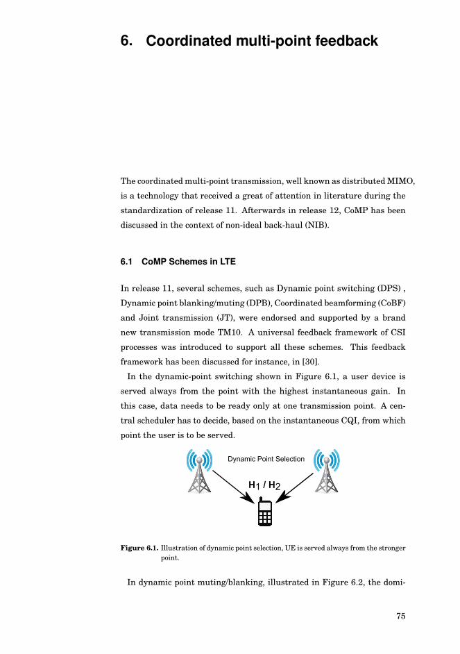
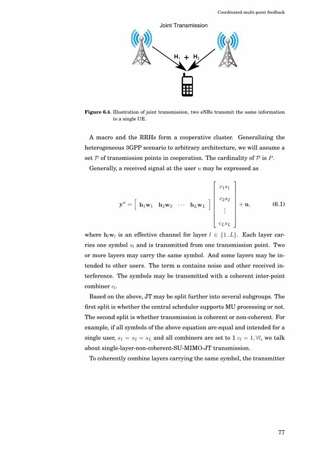
6. Coordinated multi-point feedback 75

6.1 CoMP Schemes in LTE . . . . . . . . . . . . . . . . . . . . . . 75

6.2 CoMP Feedback . . . . . . . . . . . . . . . . . . . . . . . . . . 76

7. Summary 81

References 85

Errata 93

Publications 95

4

List of Publications

This thesis consists of an overview and of the following publications which

are referred to in the text by their Roman numerals.

I Määttänen Helka-Liina, Schober Karol, Tirkkonen Olav, Wichman Risto.

Precoder partitioning in closed-loop MIMO systems. IEEE Transactions

on Wireless Communications, Vol: 8, Issue: 8, p. 3910 - 3914, Aug. 2009.

II Schober Karol, Jänis Pekka, Wichman Risto. Geodesical codebook de-

sign for precoded MIMO systems. IEEE Communications Letters, Vol: 13,

Issue: 10, p. 773 - 775, Oct. 2009.

III Schober Karol, Renaud-Alexandre Pitaval, Wichman Risto. Improved

User-specific Channel Estimation using Geodesical Interpolation at the

Transmitter. IEEE Wireless Communications Letters, Vol: 4, Issue: 2,

p. 165 - 168, Jan 2015.

IV Schober Karol, Wichman Risto, Roman Timo. Layer arrangement for

single-user coordinated multi-point transmission. In 2012 46th Annual

Conference on Information Sciences and Systems (CISS) , Princeton, NJ,

p. 1-5, Mar. 2012.

V Schober Karol, Wichman Risto, Koivisto Tommi. Refinement of MIMO

limited-feedback using second best codeword. In IEEE 2009 20th Inter-

national Symposium on Personal, Indoor and Mobile Radio Communi-

cations, Tokyo, Japan, p. 2529 - 2533, Sep. 2009.

5

List of Publications

VI Schober Karol, Määttänen, Helka-Liina, Tirkkonen Olav, Wichman

Risto. Normalized covariance matrix quantization for MIMO broadcast

systems. In 11th European Wireless Conference 2011 - Sustainable Wire-

less Technologies (European Wireless), Vienna, Austria, p. 1 - 6, Apr.

2011.

VII Schober Karol and Wichman Risto. MIMO-OFDM Channel Estima-

tion with Eigenbeamforming and User-Specific Reference Signals. In

IEEE 69th Vehicular Technology Conference, Spring 2009, Barcelona,

Spain, p. 1 - 5, Apr. 2009.

VIII Schober Karol, Wichman Risto, Koivisto Tommi. MIMO Adaptive

Codebook for Closely Spaced Antenna Arrays. In 19th European Signal

Processing Conference (EUSIPCO 2011), Barcelona, Spain, p. 1 - 5, Sep.

2011.

IX Schober Karol, Wichman Risto, Koivisto Tommi. MIMO adaptive code-

book for cross-polarized antenna arrays. In 2013 IEEE 24th Interna-

tional Symposium on Personal, Indoor and Mobile Radio Communica-

tions, London, UK, p. 1 - 5, Sep. 2013.

X Schober Karol, Mihai Enescu, Risto Wichman. Geodesical Refinement

of MIMO Limited Feedback. In IEEE Transactions on Communications,

Vol: 64, Issue: 3, p. 1031 - 1041, Jan. 2016.

6

Author’s Contribution

Publication I: “Precoder partitioning in closed-loop MIMO systems”

Author drafted chapter IV and designed the quantizations for the Gras-

mannian and Orthogonalization codebooks.

Publication II: “Geodesical codebook design for precoded MIMOsystems”

The author wrote the first draft, derived the theoretical studies and per-

formed all computer simulations.

Publication III: “Improved User-specific Channel Estimation usingGeodesical Interpolation at the Transmitter”


formed the computer simulations. The tangent space of the Flag manifold

was provided by D.Sc (Tech.) Renaud-Alexandre Pitaval.

Publication IV: “Layer arrangement for single-user coordinatedmulti-point transmission”

The author produced the first written draft, derived the theoretical stud-

ies and performed all computer simulations.

7

Author’s Contribution

Publication V: “Refinement of MIMO limited-feedback using secondbest codeword”


formed the computer simulations.

Publication VI: “Normalized covariance matrix quantization forMIMO broadcast systems”



Publication VII: “MIMO-OFDM Channel Estimation withEigenbeamforming and User-Specific Reference Signals”



Publication VIII: “MIMO Adaptive Codebook for Closely SpacedAntenna Arrays”



Publication IX: “MIMO adaptive codebook for cross-polarizedantenna arrays”



Publication X: “Geodesical Refinement of MIMO Limited Feedback”



8

Symbols and Abbreviations

Acronyms

2D two-dimensional

3D three-dimensional

3GPP The 3rd Generation Partnership Project

5G 5th generation

AAS active antenna systems

AoA angle of arrival

AoD angle of departure

BD block diagonalization

BER bit error rate

BLER block error rate

CA carrier aggregation

CCI co-channel interference

CDF cumulative density function

CDI channel direction information

CM constant modulus

CoBF coordinated beamforming

CoMP coordinated multi point

CP cyclic prefix

CQI channel quality index

9


CRS common reference signals

CS coordinated scheduling

CSI channel state information

CSI-RS channel state information reference signals

DCB double codebook

DCC double description coding

DMRS demodulation reference signals

DPB dynamic point blanking

DPC dirty paper coding

DPS dynamic point selection

DRS dedicated reference signals

DVB-T Digital Video Broadcasting, Terrestrial

eNB evolved Node B

FD-MIMO full dimension MIMO

FDD frequency division duplex

FFT fast Fourier transform

GoB grid of beams

GPS global positioning system

IEEE Institute of Electrical and Electronics Engineers

IID independent and identically distributed

IMR interference measurement resource

IoT internet of things

IRC interference rejection

ITU International Telecommunication Union

JT joint transmission

LMMSE linear minimum mean square error

10


LoS line-of-sight

LSP large scale parameter

LTE Long Time Evolution

MCS modulation and coding scheme

MDC multi description coding

METIS2020 Mobile and wireless communications Enablers for Twenty-

twenty (2020) Information Society

MISO multi input single output

ML maximum likelihood

MMSE minimum mean square error

MP multi point

MRC maximum ratio combining

MSE mean square error

MU-MIMO multi-user multiple-input-multiple-output

MUST multi-user superposition coding

NIB non-ideal backhaul

NLoS non-line-of-sight

OCI other cell interference

OFDMA orthognal frequency division multiple access

PDSCH pysical downlink shared channel

PM precoding matrix

PMCH physical multicast channel

PMI precoding matrix index

PRB physical resource block

PSK phase shift keying

R-ML reduced maximum likelihood

RE resource element

11


RRH radio remote head

RS reference signals

SC single-cell

SCM spatial channel model

SFN single frequency network

SIC successive interference cancellation

SINR signal to interference and noise ratio

SLNR signal-leakage-to-noise precoding

SQ scalar quantization

SVD singular value decomposition

TDD time division duplex

TM transmission mode

UBF unitary beamforming

ULA uniform linear array

UMTS universal mobile telecommunications system

VQ vector quantization

WINNER Wireless World Initiative New Radio

ZF-BF zero-forcing beamforming

Greek Symbols

Γ(•) geodesic

Δ horizontal space

η(•) horizontal lift

Π vertical space

ρf (•) frequency correlation function

ρt(•) time correlation function

σ(•) affine cross-section

12


Roman Symbols

E(•) expectation

FL Flag manifold

G Grassmannian manifold

H channel matrix

J(•) cost function

L number of layers

Nb number of neighboring beam in a codeword

Nr number of receive antennas

Nt number of transmit antennas

ST Stiefel manifold

U unitary group

W precoding matrix

Other Symbols

(•)∗ conjugate

(•)H hermitian transpose

(•)T transpose

∗ convolution

∠ angle of a complex number

det(•) determinant

exp(•) matrix exponential

logb logarithm of base b

� Hadamard product

⊗ Kronecker product

Re (•) real part of a complex number

Tr(•) matrix trace

vec(•) vectorization of a matrix

13


14

1. Introduction

The wireless industry is continuously evolving, trying to satisfy the in-

creasing bit-rate demand. This demand is a consequence of the growing

number of mobile devices, such as tablets, smart-phones and laptops. Fur-

thermore, it is expected that in the near future, things around us will be-

come connected as well, forming the internet of things (IoT), a network

with billions of devices all interconnected in the smart cities of the future.

Although the physical layer nowadays performs close to Shannon capac-

ity limits, even a modest improvement can significantly improve system

performance. In a cellular network, modest physical layer improvements

may be amplified. When a cell serves a terminal faster, within saved time

it may switch off and such avoid causing interference for other network

terminals. Other terminals obviously benefit from the improved interfer-

ence conditions. Improved throughput results again into shorter serving

time and increases the possibility of an empty cell, which decreases inter-

ference levels.

There exist several approaches how to increase data rates on the physi-

cal layer. The most straight-forward link-level approach is the extension

of communication spectrum, if available. This approach has been used, for

example, in 3GPP LTE Release 10-13 system [1] under the name Carrier-

aggregation (CA) [2] and is applicable also in the future, when moving to

mm-waves (30-300GHz), where a sufficient amount of resources is avail-

able. Another approach is to increase capacity by multiplexing users at

the same time-frequency resource. This can be implemented:

• in power/bit domain, by removing the signal targeted for companion

user using successive-interference-cancellation (SIC) [3] or a maximum-

likelihood (ML) receiver [4]. These are known as multi-user superposi-

tion transmission (MUST).

15

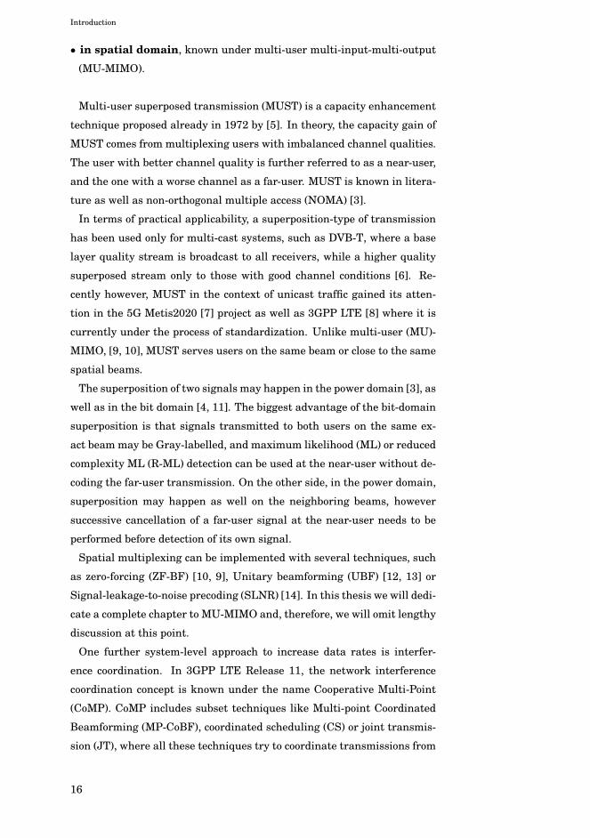
Introduction

• in spatial domain, known under multi-user multi-input-multi-output

(MU-MIMO).

Multi-user superposed transmission (MUST) is a capacity enhancement

technique proposed already in 1972 by [5]. In theory, the capacity gain of

MUST comes from multiplexing users with imbalanced channel qualities.

The user with better channel quality is further referred to as a near-user,

and the one with a worse channel as a far-user. MUST is known in litera-

ture as well as non-orthogonal multiple access (NOMA) [3].

In terms of practical applicability, a superposition-type of transmission

has been used only for multi-cast systems, such as DVB-T, where a base

layer quality stream is broadcast to all receivers, while a higher quality

superposed stream only to those with good channel conditions [6]. Re-

cently however, MUST in the context of unicast traffic gained its atten-

tion in the 5G Metis2020 [7] project as well as 3GPP LTE [8] where it is

currently under the process of standardization. Unlike multi-user (MU)-

MIMO, [9, 10], MUST serves users on the same beam or close to the same

spatial beams.

The superposition of two signals may happen in the power domain [3], as

well as in the bit domain [4, 11]. The biggest advantage of the bit-domain

superposition is that signals transmitted to both users on the same ex-

act beam may be Gray-labelled, and maximum likelihood (ML) or reduced

complexity ML (R-ML) detection can be used at the near-user without de-

coding the far-user transmission. On the other side, in the power domain,

superposition may happen as well on the neighboring beams, however

successive cancellation of a far-user signal at the near-user needs to be

performed before detection of its own signal.

Spatial multiplexing can be implemented with several techniques, such

as zero-forcing (ZF-BF) [10, 9], Unitary beamforming (UBF) [12, 13] or

Signal-leakage-to-noise precoding (SLNR) [14]. In this thesis we will dedi-

cate a complete chapter to MU-MIMO and, therefore, we will omit lengthy

discussion at this point.

One further system-level approach to increase data rates is interfer-

ence coordination. In 3GPP LTE Release 11, the network interference

coordination concept is known under the name Cooperative Multi-Point

(CoMP). CoMP includes subset techniques like Multi-point Coordinated

Beamforming (MP-CoBF), coordinated scheduling (CS) or joint transmis-

sion (JT), where all these techniques try to coordinate transmissions from

16

Introduction

various transmission points in the network and in such a way minimize

the interference. These approaches require information exchange between

transmission points as well as an increased amount of feedback from ter-

minals.

Even though feedback design for MIMO systems has been heavily inves-

tigated in the first decade of the 21st century, there are areas of MIMO

still under investigation. An example is Full-dimension(FD) / Massive

MIMO . This technology was standardized in its first version in Release 13

of 3GPP LTE. FD-MIMO is enabled by active antenna systems (AAS) [15],

where each antenna element contains its own power amplifier placed be-

hind itself. The compactness of this antenna array enables design of large

antenna arrays, forming narrow precise beams in horizontal as well as

vertical domains, enabling a high degree of spatial multiplexing and en-

ergy steering. AAS requires only baseband feed and, therefore, reduces

installation costs. The codebook for AAS has been standardized in Re-

lease 13. This codebook employs a double structure, where the long-term

wide-band part of the codebook is based on Kronecker product of hori-

zontal and vertical DFT vectors. The Kronecker structured codebook for

AAS was studied as well in [16]. Authors in [16] identified limitations

in the Kronecker structure, when there is more than one dominant beam

present in a MIMO channel. As an enhancement, authors propose pre-

coding codewords being a linear combination of DFT vectors.

1.1 Objectives and goals

The goal of this thesis is to develop efficient feedback for MIMO systems,

and its variations with respect to SU-MIMO, MU-MIMO and CoMP. The

codebook design is a key research topic of this thesis. We study the code-

book design for uncorrelated as well as correlated spatial channels, as

well as MU-MIMO related codebook design and specific design for lin-

ear receivers. The other goal of the research is the design of successive

feedback refinement for temporally-correlated channels. When a chan-

nel is slowly changing, and there is enough feedback capacity, the user

reporting precoder from a course codebook can send refinement informa-

tion for the previously reported codeword. This is similar to a one-step

differential feedback. We propose one low complex well performing solu-

tion suitable for industrial systems. One chapter of this thesis discusses

channel estimation on user-specific reference signals. The application of

17

Introduction

spatial precoders on reference signals creates a channel discontinuity and

can as well change the correlation properties of a channel. This topic has

not been studied much in academics, but is clearly a practical issue in a

wireless system employing user-specific reference symbols.

1.2 Background and contribution

MIMO systems with frequency division duplex (FDD) require channel

state information (CSI) to be fed back from a receiver to a transmitter. The

need for such a feedback is a consequence of independent fading of uplink

and downlink channels. Communication systems employing CSI feedback

are closed-loop MIMO systems. Contrary to FDD, in time division duplex

(TDD), the uplink and downlink channels are considered reciprocal when

transmitter and receiver chains are calibrated. In TDD, feedback is re-

placed by the terminal transmitting sounding reference symbols in the

uplink, aiding reciprocal channel estimation at the transmitter.

CSI can be fed back explicitly, i.e each channel component absolute value

and phase is quantized directly or jointly and fed back. This approach has

one major drawback. It does not include receivers processing capabil-

ity within the feedback. Alternatively, industrial systems such as IEEE

802.11n [17] and 3GPP LTE Release 8-13 [8] implemented implicit signal-

ing. In this type of signaling, a jointly quantized semi-unitary precoding

matrix index (PMI) is selected by the receiver along with a channel qual-

ity indicator (CQI) and fed back to a transmitter. CQI is expressed as a

modulation and coding scheme (MCS) class selected by the user terminal

from a predefined set of MCS classes.

With the implicit feedback, the CSI at the receiver is preferably quan-

tized jointly and is normalized to a power of one. This allows a good split

between the power of the channel and its spatial channel direction (CDI).

Furthermore, each stream/layer is transmitted on the orthogonal layer,

which minimizes inter-stream interference between layers. As a conse-

quence, the precoding-space is distributed on a curved space represented

by the Grassmanian manifold or, in some cases, the Stiefel/Flag mani-

fold if unitary rotation of precoding matrix subspace matters, which is

addressed in Publication I.

In SU-MIMO, the transmitter uses the user’s latest reported PMI to

spatially precode data intended for the user. This does not hold anymore

with MU-MIMO. In MU-MIMO, the transmitter tries to minimize inter-

18

Introduction

ference to a co-channel user and, therefore, modifies the reported PMI.

The most known MU-MIMO transmit processing scheme is zero-forcing

beamforming (ZF-BF). It has been developed originally for single-layer

and its extension to more transmit layers per user is called block diago-

nalization (BD). However, in both ZF-BF and BD, the number of transmit-

ted data streams should be equal to the number of receive antennas. To

allow a different number of data streams and number of antennas, sev-

eral strategies can be applied. Firstly, the user may fix receive-filter and

feedback only eigenmode(s) [18]. Fixing the receive-filter is however not

wise. The optimal receive filter at the time of transmission may be dif-

ferent from the one used at the time of feedback report. Receiver chain

phases may drift, or interference may change as well over time. Secondly,

the user may be aware of co-channel interference and suppress this in-

terference on sub-carrier bases using e.g. an LMMSE/IRC receiver. The

second solution has been adopted by LTE Release 10 standard. Finally,

the user may optimize the receive and transmit filter jointly, which is

referred to as Single-cell Coordinated beamforming (SC-CoBF). A coor-

dinated beamforming optimum can be obtained by iterative algorithms.

However, these are not preferred by practical systems, because their pro-

cessing complexity and delay is higher compared to closed-form solutions.

One closed-form solution for SC-CoBF called the Generalized eigenvalue

algorithm has been introduced in [19]. This algorithm requires the feed-

back of normalized channel covariance matrix instead of CDI and uses an

MRC receiver for reception. The strategy for direct quantization of such

a normalized covariance matrix has been proposed in an original publica-

tion for two transmit antennas [19] and extended to an arbitrary number

of antennas in [20]. Alternative quantization, proposed in Publication VI

quantizes separately eigenvalues and CDI and allows flexible trade-off be-

tween bits invested in eigenvalues and CDI. Furthermore, Publication VI

shows that importance of eigenvalues depends on antenna configuration.

For every channel-source there exists an optimal quantization given a

metric. The most general channel component source is independent and

an identically distributed (IID) Gaussian source. This type of channel

serves well for analysis purposes, however does not correspond well to

real life channels experiencing spatial-correlation. The precision of chan-

nel models has been developed hand-in-hand with increasing computa-

tional availability. Firstly, the simple Kronecker channel model described

e.g. in [21] has been used for evaluation of MIMO systems. Later, it

19

Introduction

has been replaced by more complex full spatial cluster based models,

such as SCM [22] and WINNER II [23], and in the future high-complex

ray-tracing channel models, such as Winprop, are expected to be a base-

line for system and link performance evaluation in 5G. In the Kronecker

model, spatial correlation is created by the Kronecker product between

the square-root of the correlation matrix and the MIMO independent chan-

nel components of the Gaussian distribution. This model has no geo-

metrical structure background. Contrary, the full spatial channel models

contain channel correlation implicitly as a consequence of realistic clus-

ter/obstacles in the space. As a consequence, antenna separation as well

as the angular spread of a channel influence the instantaneous spatial

correlation. We will discuss channel models more in Chapter 3.

The channel model source determines the distribution of subspaces on

a manifold. To learn more about manifolds please refer to Chapter 2. In

case of IID Gaussian distribution with unit variance and zero mean, sub-

spaces/points on the Grassmannian manifold are distributed uniformly.

An efficient way to design optimal codebooks for uniform distributions

is a geodesical packing algorithm introduced in Publication II. In addi-

tion to coherent MIMO precoding, Grassmannian packings may form a

transmit symbol constellation used for non-coherent MIMO communica-

tion [24]. However, when spatial correlation is present in the channel, a

different optimal codebook can be designed given that correlation. There-

fore, an optimal codebook should adapt to the actual channel source. The

first proposed solution to adapt to a transmit correlation matrix was pro-

posed in [25], all codewords of the uniform IID codebook are transformed

by square-root of estimated transmit-correlation matrix. This elegant so-

lution, however, has one major issue preventing it from being used in

industrial standards. Such a transformation cannot guarantee that the

transformed codebook keeps its components constant modulus, nor can

guarantee that two-layer codebook codewords stay orthogonal. Constant

modulus property was and is an important codebook property that lowers

the codeword selection complexity at the receiver. In order to enable an

adaption of the codebooks in the wireless standards an alternative solu-

tion, called a double codebook, was invented and standardized. The final

codeword is computed as a simple product of two codewords selected from

two codebooks of a specific structure. One codeword is selected wideband

and with long periodicity and the other one is selected sub-band and with

short periodicity. Double codebook optimization for uniform linear arrays

20

Introduction

is proposed in Publication VIII and for cross-polarized arrays in Publi-

cation IX. Codebook design for industry is discussed in more detail in

Chapter 4.

MU-MIMO and SU-MIMO systems with temporally-correlated channels

benefit from more precise feedback. A straightforward solution to improve

CSI at the transmitter is to invest more bits in a codebook. Unfortunately,

codeword selection complexity grows exponentially with codebook size. To

keep the size of the codebook low, CSI can be refined by a codeword from

a refinement codebook. Several techniques deal with the design of refine-

ment [26, 27, 28, 29]. In addition, a low complex refinement technique

has been proposed in Publication V and Publication III. This technique

uses geodesical interpolation to the m-th best codeword. Further details

on codebook refinement techniques will be presented in Section 5.4.

In order to receive spatially precoded data coherently, data are trans-

mitted together with reference symbols that aid the channel estimation.

The channel estimation may be carried out in two different ways. Firstly,

the channel at the receiver may be estimated for a full/clean MIMO spa-

tial channel that is consequently multiplied by the spatial precoder used

for data transmission. This approach requires knowledge of the used spa-

tial precoder at the receiver, however only one set of reference symbols is

needed for both PMI feedback estimation and data reception. Secondly, an

effective channel may be estimated directly if the transmitter applies the

same PMI used for the data as well the reference symbols. In this case,

the reference symbols are user-specific and the transmitter does not need

to inform the user about the spatial precoder applied to the data. More-

over, with user-specific reference symbols, feedback overhead scales with

the number of data streams transmitted. On the other side, one set of

reference symbols is needed for data reception and another set is needed

for feedback estimation.

User-specific RS allow the transmitter to apply a precoder of its own

choice. In TDD, where the reciprocal channel may be available at the

transmitter, Eigenbeamforming may be applied. Eigenbeamforming uses

dominant singular vector(s) to spatially precode the transmitted data. As

a consequence, neighboring sub-carriers may be precoded with a different

spatial precoder. This changes the characteristics of the user-specific pre-

coded channel. Particularly, coherence bandwidth may decrease as sud-

den artificial changes in phase and amplitude may occur between neigh-

boring sub-carriers. These coherence issues were addressed in Publica-

21

Introduction

tion VII where we proposed an algorithm to maximize the coherence band-

width of the spatially precoded channel.

In LTE, for transmission modes introduced from Release 10 onwards,

user-specific reference symbols are transmitted to aid data channel es-

timation. Furthermore, the spatial precoder is forced to be the same

within a block of 12 subcarriers (physical resource block, a PRB). There-

fore, similar amplitude and phase discontinuities, as in Eigenbeamform-

ing between sub-carriers, exist as well between PRBs. These disconti-

nuities are called the channel estimation edge effect and allow channel

estimation only within this one PRB. Lack of frequency domain interpola-

tion between reference symbols motivated the LTE system to adopt PRB

bundling. Bundling guarantees that three neighboring PRBs are precoded

with the same precoder. However, PRB bundling is not the best solution.

In Publication III, we proposed a geodesical interpolation of fed-back fre-

quency selective PMIs and showed that channel estimation performs bet-

ter than with PRB bundling. Furthermore, we provided a way how to

generate a geodesic on a Flag manifold and showed that a Flag-manifold

geodesic PMI interpolation is more suitable for two-layer transmission

than a Grassmanian- and Stiefel-manifold geodesic interpolation.

Recently, coordinated multipoint (CoMP) systems collected a lot of atten-

tion while being standardized in Release 11 of 3GPP LTE. An overview of

CoMP technology in LTE Release 11 has been well summarized in [30].

In CoMP, transmission from different points is coordinated and such in-

terference in the network is minimized. One CoMP technology subgroup

is coordinated scheduling (CS), where the user reports channel quality

feedback CQI for several of the strongest points. This CQI knowledge be-

comes global in network and the global scheduler has knowledge about

what interference it causes to users across the network when performing

scheduling. Other CoMP subgroups are multi-point coordinated beam-

forming (MP-CoBF), where PMI for several transmission points is fed

back to the global scheduler. The users for a specific time-frequency re-

source are selected so that one transmission point serves its user within

the user’s signal space and at the same transmits to the null space of the

users served by other transmission points. The most complicated CoMP

technology subgroup is joint transmission (JT). One user is served by mul-

tiple points at the same time. JT technology improves significantly cell-

edge user performance, however at the same time, it is very sensitive to

the timing advance of the signals and the transmission data have to be

22

Introduction

distributed across the transmission point in cooperation.

Each of above mentioned CoMP techniques needs a different type of

feedback. The user, however cannot know which scheme will be selected

by the network and would have to feedback CSI for all schemes, causing

high uplink overhead in the network. Therefore, in LTE, unified feedback

supporting all schemes was designed. In LTE Release 11, the user re-

ports PMI and CQI per configured transmission points, while additional

inter-point feedback will be under discussion in future releases. Per-point

PMI feedback is scalable and flexible, and has been studied e.g. in [31].

Additional inter-point feedback, such as a PMI combiner, was shown to

be beneficial in [32]. Another form of additional inter-point feedback is

layers arrangement across points, which has been studied in Publication

IV and shown to bring sufficient performance gains with only moderate

feedback. CoMP is discussed in more detail in Chapter 6.

1.3 Contribution summary

Publication I - suggests precoding space partitioning into the Grassman-

nian and the Orthogonalization parts, and shows that feedback bits can be

more efficiently used by quantizing separately the Grassmannian and the

Orthogonalization parts of a precoder with linear receivers and especially

with correlated channels.

Publication II - presents an expansion-compression algorithm (ECA) for

finding packings of points on the Grassmannian manifold using various

distance metrics. With a certain distance-metrics, the algorithm tends to

get stuck and, therefore, compression is required in addition to expansion.

Publication III - shows how geodesical precoder interpolation at the

transmitter may improve channel estimation at the receiver by removal

of the boundary artifacts of channel estimation at the receiver side. The

precoder interpolation is performed on the Flag, Stiefel and Grassman-

nian manifolds by means of geodesic. An interative algorithm to design a

geodesic on the Flag manifold using boundary conditions is proposed.

Publication IV - proposes co-phasing feedback for coordinated multi-

point joint transmission along with the selection of layers for each trans-

mission point showing that it brings sufficient performance gains with

only moderate feedback.

Publication V - proposes geodesic interpolation between the first and

second best precoding matrices as a mechanism for providing successive

23

Introduction

refinement of a feedback precoding matrix. Presents a closed-form so-

lution for an optimal interpolation parameter to maximize the received

power at the receiver. Simulation gains in LTE context are presented for

SU-MIMO.

Publication X - proposes geodesic interpolation between the first and

mth best precoding matrices as a mechanism for providing successive re-

finement of a feedback precoding matrix. In addition, this publication

derives an upper-bound of an optimal interpolation parameter, which can

be computed from fed-back CQI values at the transmitter. Simulation

gains in a LTE context are presented for MU-MIMO.

Publication VI - presents a new quantization scheme for a normalized

Wishart matrix. This scheme quantizes separately eigenvalues and CDI

and allows flexible trade-off between bits invested in eigenvalues and

CDI. It is shown that the importance of eigenvalues depends on antenna

configuration.

Publication VII - proposes a new method for retaining phase continuity

in the frequency domain after UE specific SVD beamforming is used. Sev-

eral methods to retain continuity are presented and their impact on the

channel frequency correlation is studied.

Publication VIII - proposes an optimization of a product codebook for

uniform-linear-arrays, with W1 representing long-term spatial correla-

tion properties and W2 representing short term/polarization/narrowband

properties and provides gains over the existing LTE codebook.

Publication IX - proposes an optimization of a product codebook for cross-

polarized arrays, with W1 representing long-term spatial correlation prop-

erties and W2 representing short term/polarization/narrowband proper-

ties and provides gains over the existing LTE codebook

1.4 Structure of the thesis

Further in the thesis, we introduce the reader to a MIMO-relevant mani-

fold theory and to geodesic construction on manifolds in Chapter 2. After-

wards, we discuss channel models and user-specific channel estimation in

Chapter 3. The codebook design is discussed in Chapter 4. Chapter 5 in-

troduces MU-MIMO techniques and successive feedback refinement and

Chapter 6 briefly addresses the coordinated-multipoint (CoMP). The the-

sis is concluded in Chapter 7.

24

2. Manifold theory

Manifolds are closer to us than we think. All our life we walk on Earth,

a manifold. And in fact, we exist in a curved space-time, introduced by

Einstein, which is nothing else than a manifold, a pseudo-Riemannian

manifold. So what is that manifold?

By definition, a manifold is a topological space. Each point’s neigh-

borhood on the n-dimensional manifold is homeomorphic (similar) to n-

dimensional Euclidean space. For example, each point’s neighborhood on

the 2-sphere is homeomorphic to an Euclidean plane [33], a chart. If a

point’s neighborhood is similar enough to a linear space, it becomes a dif-

ferentiable manifold. Further, if a Riemannian metric exists on the man-

ifold, it becomes a Riemannian manifold. A Riemannian metric defines a

scalar product between the vectors of tangent space, smoothly depending

on the point on the manifold [34]. An example of a Riemannian manifold

is the already mentioned unit two-dimensional sphere embedded in E3

Euclidian space. Expressing the distance measure ds2 = dx2+dy2+dz2 in

spherical coordinates as ds2 = r2dθ2 + r2 sin θ2dφ2, and setting the radius

to r = 1. The scalar product is

G =

⎡⎢⎣ 1 0

0 sin θ2

⎤⎥⎦ . (2.1)

We can notice that the scalar product 1) depends on θ 2) is always positive

and 3) is a smooth function of θ.

In this chapter we will discuss only Riemannian manifolds relevant to

MIMO systems. In Section 2.1 we will introduce Stiefel, Grassmannian

and Flag manifolds, and in Section 2.2 we will construct geodesics on

these manifolds. The construction of a geodesic is a prerequisite in our

publications PII, PIII and PX.

25

Manifold theory

2.1 Manifolds in MIMO

In precoded MIMO systems with equal transmit power per layer, a set of

all precoding matricesW for L layers transmitted over channelH with Nt

transmit antennas and Nr receive antennas is represented by a complex

Stiefel manifold ST (Nt, L), i.e.

ST (Nt, L) = {Y ∈ CNt×L|YHY = IL}, (2.2)

where L < Nt. The Stiefel manifold becomes a unitary group

U(Nt) = {U ∈ CNt×Nt |YHY = YYH = INt} (2.3)

when L = Nt.

However, the Stiefel manifold is not the manifold we are interested in,

because some points W on the Stiefel manifold are equivalent with re-

spect to MIMO closed-loop capacity C. The capacity of an instantaneous

MIMO channel H precoded by a spatial-precoder W can be expressed as

C = log2[det

(Ip +UH

LWHHHRHWUL

)], (2.4)

where R is a source-symbol covariance matrix and UL is an arbitrary

matrix from a unitary group U(L). Equation (2.4) shows that ∀UL ∈ UL,

capacity C is the same, because the determinant of a unitary matrix is one

and det(I+XY) = det(I+YX). A manifold, where points are equivalent

with respect to right unitary rotation by U(L), is called a Grassmannian

manifold, and is denoted as the quotient space of a Stiefel manifold

G(Nt, L) ∼= ST (Nt, L)/U(L). (2.5)

The capacity expressed in (2.4) assumes the presence of a non-linear

receiver, such as maximum likelihood, which can decouple MIMO layers.

However, user-terminals are often equipped only with linear receivers,

which are of modest complexity. In PI we have shown that with a linear

MMSE receiver, the capacity of a system is non-equivalent to right rota-

tion from right UL, while still equivalent to column phase rotation rep-

resented by a space of unitary diagonal matrices Udp. Therefore, matrices

W1 and W2 are equivalent if W1 = W2Udp = W2diag(e

jθ1 , ejθ2 , · · · , ejθL)).Such an equivalence class can be expressed as a general Flag manifold

FL(n, [p1, p2, ..., pL]) (2.6)

described in [35], where p1 = p2 = ... = pL = 1 further denoted as

FL(Nt, L). A Flag manifold can be expressed as the quotient space of

26

Manifold theory

a Stiefel manifold

FL(Nt, L) ∼= ST (Nt, L)/U(1)L. (2.7)

In case L = 1, the Flag manifold FL(Nt, 1) is equivalent to the Grass-

mannian manifold FL(Nt, 1) ∼= G(Nt, 1). The three manifolds are of differ-

ent cardinality and the relation between them can be expressed as

G(Nt, L) ⊂ FL(Nt, L) ⊂ ST (Nt, L). (2.8)

2.2 Geodesics on the MIMO-relevant manifolds

Now when we defined MIMO manifolds, we can introduce geodesics on

them. We will start geodesic construction on a unitary group, to start

with the simplest case.

A unitary group U(Nt) is a set of unitary matrices of dimension Nt ×Nt, and every unitary matrix may be expressed by an exponential map

U = exp (X), where X is a skew-hermitian matrix and exp is a matrix

exponential

exp (X) =

∞∑k=0

1

k!Xk. (2.9)

A geodesic Γ on the manifold is a line that preserves tangent space.

Tangent space for a unitary group U(Nt) can be found easily [36] by dif-

ferentiating UHU = I, which yields UHU + UHU = 0. This means that

UHU must be a skew-hermitian matrix. A geodesic equation is an equa-

tion satisfying ΓHΓ = X, where X is a constant matrix. Such an equation

is

Γ(p) = U(0) exp (pX), (2.10)

where p tracks the geodesic. Having a geodesic equation for a manifold/set

of all unitary matrices, a unitary group, we may obtain geodesics as well

for the quotient spaces of the unitary group.

The Stiefel manifold ST (Nt, L) from (2.2) is a quotient space of U(Nt).

We can write Y = UINt,L, where INt,L is a matrix formed by the first L

columns of the Nt × Nt identity matrix. In other words, point Y on the

Stiefel manifold is equivalent to the set of unitary matrices having the

first L columns the same as Y. Quotient space is given by

[U] = U

⎡⎢⎣ Ip 0

0 U(Nt − L)

⎤⎥⎦ , (2.11)

27

Manifold theory

where U(Nt − L) ∈ U(Nt − L).

Now, to construct a geodesic, we need to find a tangent space to the

Stiefel manifold. The tangent space consists of a vertical space Π and a

horizontal space Δ, these spaces being complementary to each other. The

vertical space is defined as a tangent to quotient space [U], and horizontal

space is then defined as its complement [36]. The vertical space

Π = U

⎡⎢⎣ 0 0

0 C

⎤⎥⎦ , (2.12)

where C is skew-hermitian satisfies [U]HΠ +ΠH[U] = 0. The horizontal

space of the Stiefel manifold is then a complement

Δ = U

⎡⎢⎣ A −BH

B 0

⎤⎥⎦ , (2.13)

where A is a skew-hermitian matrix and B is an arbitrary matrix.

Similarly, we derive vertical and horizontal spaces for Grassmannian

and Flag manifolds. For a Grassmannian manifold a quotient space is

[U] = U

⎡⎢⎣ U(L) 0

0 U(Nt − L)

⎤⎥⎦ . (2.14)

The vertical and horizontal space of a Grassmannian manifold are then

Π = U

⎡⎢⎣ A 0

0 C

⎤⎥⎦ ,Δ = U

⎡⎢⎣ 0 −BH

B 0

⎤⎥⎦ . (2.15)

For a Flag manifold a quotient space

[U] = U

⎡⎢⎢⎢⎢⎢⎢⎢⎣

⎡⎢⎢⎢⎢⎣U1(1) 0 0

0. . . 0

0 0 UL(1)

⎤⎥⎥⎥⎥⎦ 0

0 U(Nt − L)

⎤⎥⎥⎥⎥⎥⎥⎥⎦

(2.16)

was defined in PIII. The vertical and horizontal space of a Flag manifold

are then

Π = U

⎡⎢⎢⎢⎢⎢⎢⎢⎣

⎡⎢⎢⎢⎢⎣

a1 0 0

0. . . 0

0 0 aL

⎤⎥⎥⎥⎥⎦ 0

0 C

⎤⎥⎥⎥⎥⎥⎥⎥⎦,Δ = U

⎡⎢⎢⎢⎢⎢⎢⎢⎣

⎡⎢⎢⎢⎢⎣

0 −f∗1 −f∗

2

f1. . . −f∗

n

f2 fn 0

⎤⎥⎥⎥⎥⎦ −BH

B 0

⎤⎥⎥⎥⎥⎥⎥⎥⎦.

(2.17)

28

Manifold theory

The geodesic on a manifold, according to [36], given a tangent vector in

horizontal space H ∈ Δ is

Γ(p) = U(0) exp (pH)INt×L, (2.18)

where Δ is as in (2.13),(2.15) and (2.17).

However, in MIMO communications H is typically not known. Instead,

we have typically two boundary points of a geodesic. In case of a Grass-

mannian manifold, the horizontal space is simple, and there exists a closed

form solution to derive H from two boundary points/precoders W1 and

W2.

According to PII, a geodesic between the two points W1 and W2 on the

Grassmannian manifold can be constructed by finding η(W2)W1 , a hori-

zontal lift of W2 at W1, which lies in the tangent (orthogonal) space of

point W1. Firstly, we find the affine cross-section σ(W2) of W⊥1 and fiber

represented by W2. The affine cross-section σW1(W2) is found by solving

WH1 (σ(W2) −W1) = 0, i.e. by setting σW1(W2) = W2(W

H1W2)

−1. Sec-

ondly, we compute the horizontal lift by projecting the affine cross-section

σ(W2) onto the orthogonal space of W1,

η(W2)W1 = (I−W1WH1 )σW1(W2) = σW1(W2)−W1, (2.19)

which has the singular value decomposition (SVD) U(tanΦ)VH , where U

is an orthogonal complement ofW1,Φ is a diagonal matrix of the principal

angles and V is a square unitary matrix. Finally, the geodesic from point

W1 towards point W2 having η(W2)W1 is given by [37]

Γ(p) =W1V cos(Φp) +U sin(Φp), (2.20)

where p tracks the geodesic Γ, that is Γ(0) ∼ W1 and Γ(1) ∼ W21, and ∼

stands for the equivalence relation.

The geometry of geodesic construction on real G(2, 1) is illustrated in the

Figure 2.1.

There exists an alternative way of constructing the geodesic on the Grass-

mannian manifold, based on boundary conditions. In [38], the authors

1Let us SVD decompose WH1W2 = L cos (Φ)RH and W1 = U tan (Φ)VH =

W2R1

cos (Φ)LH −W1. Further we know that U is orthogonal to W1, UHW1 = 0.

Thus, we may simplify UHU tan (Φ)VH = UHW2R1

cos (Φ)LH from which we

derive UHW2 = sin (Φ)RH and V = L. We have Γ(1) ∼ W2 if WH2 Γ(1)

is a unitary matrix. Now, WH2 Γ(1) = WH

2W1L cos (Φ) + WH2U sin (Φ) =

R cos (Φ)LHL cos (Φ) +R sin (Φ) sin (Φ) = R, which is unitary. Therefore Γ(1) ∼W2.

29

Manifold theory

W2

W1 (W2)

W1(W2)-W1

Figure 2.1. Geodesic construction on real G(2, 1)

obtain the principal angles as WH1W2 = V cos(Φ)TH. And solve (2.20) for

U as

U = [W2T−W1V cos(Φ)] sin(Φ)−1. (2.21)

Unfortunately, for Stiefel and Grassmannian manifolds, both having

more complicated horizontal spaces, a closed-form solution does not ex-

ist.

A geodesic for the Stiefel manifold using a canonical metric is defined

according to [36] as in (2.18), where horizontal space is as in (2.13).

Having only starting point W1, W⊥1 and destination point W2, in or-

der to construct geodesic between these points, it is necessary to find the

unique matrices A and B. To the best of our knowledge, those matrices

cannot be obtained in closed-form. On the other hand, an iterative al-

gorithm for a real manifold using the steepest descend algorithm for the

Stiefel manifold using an Euclidian metric was presented in [39], using

similar tools as in [39], however this time for complex Stiefel manifold

with canonical metric. We construct a cost function as

J(X) = ‖Γ(1)−W2‖2F (2.22)

and we parametrize the skew-hermitian matrix

A =

⎡⎢⎢⎢⎢⎢⎢⎢⎢⎢⎣

jt1 −tL+1 + jtL+2 · · · · · ·

tL+1 + jtL+2 jt2...

...

......

. . . −tL2−1 + jtL2

· · · · · · tL2−1 + jtL2 jtL

⎤⎥⎥⎥⎥⎥⎥⎥⎥⎥⎦

(2.23)

and arbitrary matrix

B =

⎡⎢⎢⎢⎢⎢⎣

tL2+1 + jtL2+2 · · · tL2+2(Nt−L)−1 + jtL2+2(Nt−L)

.... . .

...

t2NtL−L2−2(Nt−L)+1 + jt2NtL−L2−2(Nt−L)+2 · · · t2NtL−L2−1 + jt2NtL−L2

⎤⎥⎥⎥⎥⎥⎦.

(2.24)

30

Manifold theory

As a result, there are 2NtL − L2 real parameters. The steepest descend

algorithm requires the gradient of a cost function J(X), which we express

as

∂J(X)

∂tk= 4TrRe

((Γ(1)−W2‖)H

[W1W

⊥1

] ∂ exp(X)

∂tkIL

), (2.25)

where partial derivative of exp(X) may be computed according to [40] as

∂ expX

∂tk=

∫ 1

0exp(1− u)

∂X

∂tkexp(uA)du. (2.26)

A similar approach can be applied for the Flag manifold. The cost function

can be expressed as

J(X) = ‖WH2 Γ(1)� Γ(1)HW2 − I‖2F , (2.27)

where � is the symbol for the Hadamard product and the partial deriva-

tive is then

∂J(X)

∂tk= 4TrRe

((E�EH − I)(E� ∂Γ(1)H

∂tkW2 +WH

2

∂Γ(1)

∂tk�EH)

),

(2.28)

where E = WH2 Γ(1) is a cross-product between the desired and current

destination of the geodesic. The partial derivative ∂Γ(1)∂tk

is computed in the

same way as in equation (2.26). Now we are able to construct geodesics

on all three manifolds.

31

Manifold theory

32

3. MIMO channel properties andestimation

Knowledge of channel propagation conditions is crucial to wireless sys-

tem design; when tuning a channel estimator or designing CSI feedback.

While in particular scenarios, designed feedback may work well, in other

scenarios it might be inaccurate. For example, with cross-polarization an-

tennas, in a line-of-sight (LoS) propagation model, horizontal and vertical

polarization fades identically, while in non-line-of-sight (NLoS) , polariza-

tions fade independently. Therefore, when designing a codebook for LoS

propagation conditions, fixing a cross-polarization combiner reduces feed-

back overhead.

In the following, section 3.1 introduces channel models used across our

publications. In section 3.2, we introduce the principles of pilot-based

channel estimation in LTE. The last two sections (3.5 and 3.4) are dedi-

cated to channel estimation with eigenbeamforming in TDD systems and

with spatial precoding and user-specific reference symbols in FDD sys-

tems.

3.1 Channel models

Across publications we considered different channel models. In PI and

PII, we assumed the most simplistic channel model for Nt transmit and

Nr receive antennas, where each channel component is independent and

identically distributed (IID). A MIMO channel matrix of size Nr ×Nt is

H =1√2

⎡⎢⎢⎢⎢⎣

h1,1 . . . h1,Nt

... hr,t...

hNr,1 . . . hNr,Nt

⎤⎥⎥⎥⎥⎦ , (3.1)

where hr,t ∼ N (0, 1) + jN (0, 1) and the covariance matrices are Rt =

E[HHH] = INt and Rr = E[HHH] = INr . The random matrix HHH =

33

MIMO channel properties and estimation

QΛQH can be decomposed using economical singular value decomposi-

tion, where Q is a semi-unitary matrix of dimension Nt × Nr. We as-

sume that Nr < Nt, which is typical in practice. Since the above random

matrix H is an independent isotropically distributed (IID), Q is as well

isotropically distributed and [41] showed that all isotropically distributed

semi-unitary matrices of dimension Nt ×Nr are uniformly distributed on

the Stiefel manifold ST (Nr, Nt) defined in (2.2). The above channel model

models a non-coherent MIMO Rayleigh fading channel, with the assump-

tion that the channel is constant during the duration of the symbol period

and its realization changes from symbol to symbol. This model allows us

to express open-loop capacity [41]. In PI we applied a Kronecker model on

top of a IID channel, to model spatial correlation. The overall covariance

matrix is expressed by the Kronecker product between the transmit and

receive covariance matrices R = Rt ⊗ Rr and the transformed channel

becomes H = R1/2vec(H). Alternatively, a correlated channel can be con-

structed as well as by multiplication with the partial transmit and receive

covariance matrices H = R1/2r HR

1/2t , and if the diagonal elements of Rr

are all ones, it can be shown that

E[HHH] = E[RH/2t HHRrHR

1/2t ] = Rt, (3.2)

and similarly E[HHH] = Rr. The Kronecker channel model tends to in-

crease the channel’s degrees of freedom (DoF) leading to overestimation

of capacity [42].

The channel covariance matrix Rt resp. Rr was modeled for horizontal

Uniform linear array (ULA) using an exponential model used for instance

in [43]. The correlation matrix is expressed as

Rt =1√2

⎡⎢⎢⎢⎢⎢⎢⎢⎢⎢⎢⎢⎣

1 ρ1 ρ2 · · · ρNt−1

(ρ∗)1 1 ρ1 · · · ρNt−2

(ρ∗)2 (ρ∗)1 1 · · · (ρ∗)Nt−3

......

... . . . ...

(ρ∗)−(Nt−1) (ρ∗)−(Nt−2) (ρ∗)−(Nt−3) · · · 1

⎤⎥⎥⎥⎥⎥⎥⎥⎥⎥⎥⎥⎦, (3.3)

where correlation ρ = rejθ, r expresses the strength of the correlation

between neighboring antennas and θ expresses the spatial direction of

the correlation. In PII, the θ is uniformly distributed between 0 and 2π. It

guarantees that the channel is isotropically distributed in the azimuthal

angular domain.

34


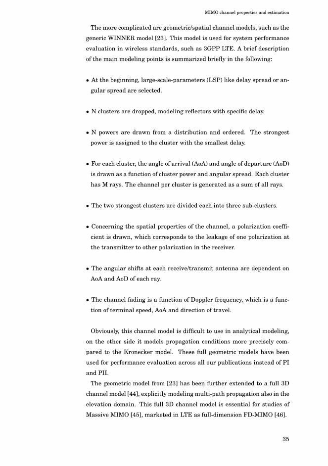
The more complicated are geometric/spatial channel models, such as the

generic WINNER model [23]. This model is used for system performance

evaluation in wireless standards, such as 3GPP LTE. A brief description

of the main modeling points is summarized briefly in the following:

• At the beginning, large-scale-parameters (LSP) like delay spread or an-

gular spread are selected.

• N clusters are dropped, modeling reflectors with specific delay.

• N powers are drawn from a distribution and ordered. The strongest

power is assigned to the cluster with the smallest delay.

• For each cluster, the angle of arrival (AoA) and angle of departure (AoD)

is drawn as a function of cluster power and angular spread. Each cluster

has M rays. The channel per cluster is generated as a sum of all rays.

• The two strongest clusters are divided each into three sub-clusters.

• Concerning the spatial properties of the channel, a polarization coeffi-

cient is drawn, which corresponds to the leakage of one polarization at

the transmitter to other polarization in the receiver.

• The angular shifts at each receive/transmit antenna are dependent on

AoA and AoD of each ray.

• The channel fading is a function of Doppler frequency, which is a func-

tion of terminal speed, AoA and direction of travel.

Obviously, this channel model is difficult to use in analytical modeling,

on the other side it models propagation conditions more precisely com-

pared to the Kronecker model. These full geometric models have been

used for performance evaluation across all our publications instead of PI

and PII.

The geometric model from [23] has been further extended to a full 3D

channel model [44], explicitly modeling multi-path propagation also in the

elevation domain. This full 3D channel model is essential for studies of

Massive MIMO [45], marketed in LTE as full-dimension FD-MIMO [46].

35


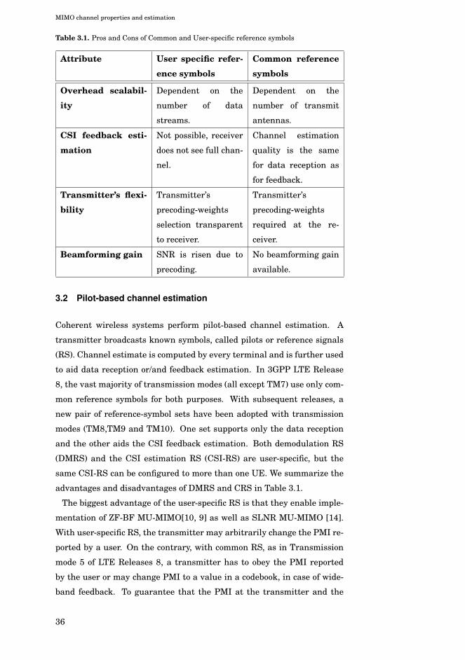
Table 3.1. Pros and Cons of Common and User-specific reference symbols

Attribute User specific refer-

ence symbols

Common reference

symbols

Overhead scalabil-

ity

Dependent on the

number of data

streams.

Dependent on the

number of transmit

antennas.

CSI feedback esti-

mation

Not possible, receiver

does not see full chan-

nel.

Channel estimation

quality is the same

for data reception as

for feedback.

Transmitter’s flexi-

bility

Transmitter’s

precoding-weights

selection transparent

to receiver.

Transmitter’s

precoding-weights

required at the re-

ceiver.

Beamforming gain SNR is risen due to

precoding.

No beamforming gain

available.

3.2 Pilot-based channel estimation

Coherent wireless systems perform pilot-based channel estimation. A

transmitter broadcasts known symbols, called pilots or reference signals

(RS). Channel estimate is computed by every terminal and is further used

to aid data reception or/and feedback estimation. In 3GPP LTE Release

8, the vast majority of transmission modes (all except TM7) use only com-

mon reference symbols for both purposes. With subsequent releases, a

new pair of reference-symbol sets have been adopted with transmission

modes (TM8,TM9 and TM10). One set supports only the data reception

and the other aids the CSI feedback estimation. Both demodulation RS

(DMRS) and the CSI estimation RS (CSI-RS) are user-specific, but the

same CSI-RS can be configured to more than one UE. We summarize the

advantages and disadvantages of DMRS and CRS in Table 3.1.

The biggest advantage of the user-specific RS is that they enable imple-

mentation of ZF-BF MU-MIMO[10, 9] as well as SLNR MU-MIMO [14].

With user-specific RS, the transmitter may arbitrarily change the PMI re-

ported by a user. On the contrary, with common RS, as in Transmission

mode 5 of LTE Releases 8, a transmitter has to obey the PMI reported

by the user or may change PMI to a value in a codebook, in case of wide-

band feedback. To guarantee that the PMI at the transmitter and the

36


receiver is identical, the transmitter sends one bit over the control chan-

nel to confirm successful reception of the user’s PMI feedback in case of

sub-band feedback, and the PMI index in case of wide-band allocation.

Figure 3.1 shows an example of LTE RS symbols in a one time-frequency

resource block. DRS corresponds to the dedicated/user-specific RS of sin-

gle ports in TM7, CRS to four ports of common RS and DMRS to two ports

of the dedicated/user-specific RS in TM9 and TM10. The RS are designed

sparsely to decrease overhead. Therefore, channel estimators have to per-

form channel interpolation.

The OFDMA channel estimate is often obtained by 2D Wiener filtering

of a 2D pilot grid in symbol-frequency domains, as shown in Figure 3.1.

Wiener filtering in the context of OFDMA channel estimation was studied

e.g. in [47, 48, 49]. The solution for 3D Wiener filtering in spatial-time-

frequency domains has been proposed in [50]. Obviously, the spatial do-

main interpolation between antennas is possible only if there exists non-

zero correlation between them. The complexity of the Wiener channel

estimation can be decreased by performing cascaded 1D channel estima-

tions, as suggested e.g. [47].

0 6time slot #0 0 6time slot #1

Freq

uen

cy d

omai

n-1

PR

B

C

C

C

C

C

C

C

C

C

C

C

C

C

C

C

C

C

C

C

C

C

C

C

C

C

C

C

C

D

D

D

DRS

D

D

D

D

D

D

D

D

D

D

D

D

D

D

DMRS

D

D

D

D

D

D

D

D

D

D

D

D

D

D

D

D

D

D

D

D

D

D

D

D

D

D

D

D

D

D

D

D

D

D

D

D

D

D

D

D

D

D

D

D

D

D

D

D

D

D

D

D

D

D

D

D

D

D

D

D

D

D

D

D

D

D

D

D

D

D

D

D

D

D

D

D

D

CRS

CRS CRS

CRS

CRS CRS

CRSCRS

CRS

CRS

CRS

CRS

CRS

CRS

CRS

CRS

CRS

CRS

CRSCRS CRS

CRS

CRS

CRS

DRS

DRS

DRS

DRS

DRS

DRS

DRS

DRS

DRS

DRS

DRS

DMRS

DMRS

DMRS

DMRS DMRS

DMRS DMRS

DMRS

DMRSDMRS

DMRS

Figure 3.1. User-specific reference symbol layout in downlink transmission mode 7 (DRS)and transmission modes 8,9,10 (DMRS 2 ports).

Precoder selection flexibility at the transmitter, is important as well for

MIMO precoding in reciprocal system, such as TDD. As mentioned earlier,

the first transmission mode using the DRS user-specific reference symbols

was TM7. This mode is intended for single-layer transmission based on

angle of arrival using TDD reciprocity. While, FDD closed-loop transmis-

sion modes using up to 8 layer DMRS user-specific reference symbols were

TM8, TM9 and TM10 in later releases.

37


3.3 System model

We consider the orthogonal frequency division multiple access (OFDMA)

downlink system. With a single transmit and receive antenna, a vector x

of Ns symbols is transformed by inverse Fast Fourier Transform (FFT) to

time domain. The time domain symbol xt is extended by the Cyclic prefix

(CP) xt = [cTt xTt ]

T and sent over the multipath channel ht. The received

signal yt is then a convolution of the channel response and transmitted

signal, i.e. yt = ht ∗ xt. If the channel response is no longer than the

duration of the CP, the time domain received signal yt transformed by

FFT to frequency, becomes a product between the channel frequency re-

sponse and transmitted symbols. Thus, we may rewrite the system model

in simplified form at each sub-carrier n as y = hx + η. For a transmitter

comprising Nt antennas and receiver Nr antennas, a simplified system

model at sub-carrier n can be expressed as

y = HWx+ η, (3.4)

where y is the received signal tall vector of dimension Nr × 1, W is the

spatial precoding matrix of dimension Nt × L and x is a tall vector of

L symbols transmitted simultaneously at the single frequency-time re-

source. The transmit power is limited to Tr(E[xxH]) = Pt and spatial

precoder is unitary WHW = I.

3.4 Channel estimation with Eigenbeamforming

With introduction of the user-specific reference symbols, user-specific chan-

nel starts to be dependent on the precoding weights used by a transmitter.

In case the same precoding weight w is used over the scheduled band-

width, the frequency correlation ρf [Δn] of the channel between two sub-

carriers of distance Δn does not change. We assume that each hi channel

component of a channel h[n] = [h1, h2, . . . , hNt ], where n ∈ [1, Nsc], has

frequency correlation ρhif [Δn] and ||w||2F = 1. The frequency correlation of

equivalent channel h = hw components ρhj

f [Δn] = ρhif [Δn], if channel com-

ponents are identically and independently distributed. In practice, the

applied spatial precoder may attenuate the path and, as such, suppress

the frequency selectivity of the channel. This results in higher channel

correlation.

Contrary to this, if precoding weights change from sub-carrier to sub-

38


carrier, the phase and amplitude correlation in the frequency domain may

change more rapidly. An example of a fast changing precoding is Eigen-

beamforming, where the main singular vector v1 of the Nr × Nt dimen-

sional channel H[n] at sub-carrier n with Lmax = min(Nt, Nr) layers is

used for precoding, where

H[n] =[u1 · · · uLmax

]⎡⎢⎢⎢⎢⎣

λ1 0 0

0. . . 0

0 0 λLmax

⎤⎥⎥⎥⎥⎦

⎡⎢⎢⎢⎢⎣

vH1...

vHLmax

⎤⎥⎥⎥⎥⎦ . (3.5)

An equivalent channel h after Eigenbeamforming (i.e. setting w = v1) for

L = 1 layer therefore becomes

h = u1λ1ejϕ, (3.6)

where u1 and λ1 are deterministic due to the realization of the channel

and ϕ can be chosen arbitrarily with respect to capacity. Selection of ϕ

is however not invariant to channel estimation at the receiver. In PVII

we addressed ϕ optimization in that context. The baseline solution which

comes immediately to mind is fixing the phase of the first equivalent chan-

nel component h1 to a real number by setting ϕ = −∠(u1(1, 1)), referred

in PVII as Method 1. This method is not the most optimal solution to the

problem. In PVII, an alternative method is suggested. This method’s goal

is to minimize channel change between two neighboring sub-carriers n

and n− 1, defining the cost function

Jn(θ) = argmin ||h[n]− h[n− 1]ejϕ[n]||2. (3.7)

Rewriting the above cost function Jn(θ) using a trace we obtain

Jn(θ) = argmaxTr{h[n]h[n− 1]He−jϕ[n] + h[n]hH[n− 1]ejϕ[n]}, (3.8)

which is maximized, if both expressions are real, i.e. when

ϕ[n] = ∠Tr{h[n]h[n− 1]H}. (3.9)

This method is referred to as the Eigenbeamforming Method 2. Firstly,

the transmitter computes the equivalent channels per each sub-carrier

using eigenvector decomposition. In the second step, the transmitter cor-

rects the overall phases ϕ[n] within the scheduled band. In order to bench-

mark these two methods we define the discrete frequency auto-correlation

function of channel component i as

ρf [Δn] = En[hi[n]h∗i [n+Δn]], (3.10)

39


−100 −50 0 50

0.1

0.2

0.3

0.4

0.5

0.6

0.7

0.8

0.9

Δn [15kHz]

|ρ|[-]

Channel component H(1,1)

Eq. channel component heq (1,1)


Figure 3.2. The correlation in frequency - Method 1. Solid line corresponds to the corre-lation of unprecoded channel tap, and dashed lines correspond to the correla-tion of channel taps of the equivalent channel.

which depends on the power-delay-profile of a channel [47, 48].

Figure 3.2 shows the absolute value of frequency-correlation for the

equivalent channel h of dimension Nr = 2, L = 1 corrected using Method 1.

The selected channel model is SCM urban macro. The correlation of the

first channel component is bigger and the correlation of the second chan-

nel component is smaller than the correlation of clean/non-precoded chan-

nel component. This asymmetry is undesirable, because two different fil-

ters would need to be pre-computed at the user equipment. Computation

of filters is a costly operation. Figure 3.3 shows the absolute value of

auto-correlation for the equivalent channel corrected by Method 2. Now

both, the first as well as the second component of the equivalent channel,

have identical correlation functions. Moreover, for both, the correlation is

higher than that of the original channel components. Method 2 requires

as well more complexity in the second step when ϕ[n]’s are computed.

However, this complexity is on the transmitter side and it is less of an

issue.

To further benchmark these two methods. We have measured the chan-

nel estimation error. As a metric we have chosen channel power to esti-

mation MSE, M =||h||2F||e||2F

. The function of geometry is shown in Figure 3.4.

Both two methods are benchmarked using theoretical Real (REAL) and

40


−50 0 50 100

0.1

0.2

0.3

0.4

0.5

0.6

0.7

0.8

0.9

Δn [15kHz]

|ρ|[-]

Channel component H(1,1)



Figure 3.3. The absolute number of correlation in frequency - Method 2. Solid line ex-presses original channel tap and Dashed lines correspond to channel taps ofequivalent channel.

Complex (CMPL) correlation functions, as well as their own method-specific

measured correlation functions (MTH1/MTH2) from Figures 3.2 and 3.3.

Irrespective of correlation function used for filter construction, Method 2

performs superior.

Yet another method, often used in practice, rotates eigenvector v1 such

that its first component becomes a real number, i.e. ϕ = −∠(v1(1, 1)).Benchmarking of Method 3 against previous methods is depicted on Fig-

ures 3.5 and 3.6 that show the measured correlation ρf [Δn], absolute

value and angle, as a function of sub-carrier difference Δn. Correlation

was measured on a generic WINNER II UMaNLoS channel model. The

performance of the two methods, Method 1 and Method 2, is comparable

to the performance shown in Figures 3.2 and 3.3 from PV II. The equiva-

lent channel h correlation of Method 3 is significantly lower than the one

of Method 2. The higher the correlation is, better the channel estimator

may average out the noise. Moreover, it is obvious from Figure 3.6 that

Method 3 adds additional phase change to the equivalent channel.

The Methods 1-3 were introduced only for a single transmitted layer. In

case more layers are transmitted to the user at the same time, each layer

can be treated separately according to the above principles.

41


0 5 10 15 205

10

15

20

25

30

35

Geometry [dB]

M[dB]

CMPL−Mth2CMPL−Mth1REAL−Mth2REAL−Mth1MTH2−Mth2MTH1−Mth1

Figure 3.4. Channel power to channel estimation error metric as function of user geom-etry with Method 1 and Method 2 Eigenbeamforming.

3.5 Channel estimation of user-specific downlink channel withlimited feedback

In FDD, to perform beamforming or spatial-multiplexing, a CSI feedback

from a receiver is required at the transmitter. Limited CSI feedback can

be in the form of a precoding matrix index (PMI), reported for full band or

sub-band of N sub-carriers. In CRS based transmission modes, eNB has to

signal used PMI or PMI confirmation to the UE in downlink control chan-

nel. Contrary, in user-specific RS-based modes, a user may be scheduled

with an arbitrary transmit PMI (tx-PMI) per sub-carrier. However, it is

beneficial to keep the same PMI over the sub-band, such that the channel-

estimator of the user-specific channel may assume channel statistics to be

constant within that band. In LTE, the smallest scheduling unit is a PRB,

i.e. 12 sub-carriers. Studying the performance of channel estimation with

one PRB tx-PMI granularity, it has been noted that the channel estimator

suffers from the so called edge-effect. The edge-effect is depicted in Fig-

ure 3.7, where angle discontinuities occur due to the change of PMI. The

channel estimator may not perform noise smoothing across PRBs. As a

solution to this problem PRB bundling was introduced in 3GPP Release

10 for TM10 (TS36.211). It sets the minimum scheduling unit to be of at

least 3PRB (in case of 10MHz system bandwidth). PRB bundling guaran-

42


0 10 20 30 40 50 60 70 80 90 1000.2

0.3

0.4

0.5

0.6

0.7

0.8

0.9

1

Δ n [15kHz]|ρ

| [−

]

heq(1,1) − Method 1






Figure 3.5. Measured correlation absolute value for all three methods and Winner IIUMaNLoS channel

0 10 20 30 40 50 60 70 80 90 100−0.2

0

0.2

0.4

0.6

0.8

1

Δ n [15kHz]

∠ρ

[rad]







Figure 3.6. Measured correlation angle value for all three methods and Winner II UMaN-LoS channel.

tees that PMI remains constant over the allocated band, which sets the

number of edges to two per scheduling unit.

There exists a better solution than PRB bundling to provide a smooth

channel over the allocated bandwidth. A geodesic interpolation at the

transmitter may smooth out the equivalent channel, while precoding gain

from limited-feedback is preserved or even improved.

Interpolation of channel state information (CSI) is a well investigated

subject. Linear interpolation for beam-forming vectors has been intro-

duced in [51] to reduce multi-input-multi-output (MIMO) precoding feed-

back. While fed back PMs are semi-unitary matrices, i.e. elements in the

Stiefel manifold; often PM performance comes from a Grassmannian in-

43


0 100 200 300 400 500 600−1

−0.8

−0.6

−0.4

−0.2

0

0.2

0.4

0.6

0.8

n

∠[ h

(1,1

)]

Angle discontinuity

Figure 3.7. Channel component angle as function of sub-carrier index. The WINNER IIUMaLoS channel realization precoded by 4tx 3GPP codebook.

terpretation. Interpolation on a Grassmann manifold for an arbitrary PM

has been proposed and investigated in [38], and in [52, 53] CSI geodesical

prediction in the receiver and interpolation at the transmitter has been

used to mitigate the effect of latency and feedback clustering. However,

in all of this mentioned work, the interpolation is targeted to improve the

spatial precoding at the transmitter, which typically brings only small

benefit. Contrary to this, in PIII we have investigated CSI interpolation

in the context of user-specific channel estimation.

Figure 3.8 illustrates the proposed PM interpolation from PIII, which

enables continuous user-specific channel estimation for a demodulation

purposes across the continuously allocated frequency band. A constant

PM is fed-back to the transmitter per cluster and we perform first-order

interpolation between neighboring PMs. The geodesic is constructed be-

tween sub-carriers located in the middles of neighboring clusters.

In PIII we have studied the impact of geodesical interpolation on user-

specific channel estimation for one-layer and two-layer transmission. We

have tried interpolation geodesics on three manifolds from Chapter 2,

namely Grassmannian, Flag and Stiefel manifolds. It turned out that

for channel estimation, Grassmannian and Flag manifold interpolation is

better than Stiefel manifold interpolation, while interpolation on a Flag

manifold better suits the MIMO systems with linear receivers. In PIII

we shown that interpolation may outperform PRB bundling in the con-

text of channel estimation. Figure 3.9 shows how BER performance is

improved compared to PRB bundling. When interpolation is performed at

44


Cluster 1 Cluster 2 Cluster 3 Cluster 4 Cluster 5 Cluster 6

frequency [SCs]

Tran

smit

ted

PM

(ill

ust

rati

ve)

A single PM for all SCs within cluster (3GPP LTE)

Interpolated PM (proposed)

uster 4 ClusClusterter 5 Clu4 5

unsmooth PM results in a small systematic channel estimation error

Figure 3.8. Illustrative example of the proposed interpolated PMs in freq. domain. Theinterpolation enables continuous ch. estimation across the full-band.

0 5 10 15 20 2510−3

10−2

10−1

SINR [dB]

BE

R

3GPP LTE Transmisison mode 9, rank 1, PMI 6PRB granularity

Ideal Ch. Est.Ch. Est. 3PRB − no interpolCh. Est. 50PRB − interpol.

16QAM

64QAM

QPSK

Figure 3.9. Link BER performance with realistic channel estimation using PRB bundlingand geodesical interpolation.

the transmitter, the receiver may perform channel smoothing across the

whole allocated bandwidth. On the other hand, however, PRB bundling

can perform channel smoothing only across 3-PRB chunks.

45


46

4. Single-user MIMO feedback

In FDD cellular systems, CSI is quantized at the user terminal and fed

back to the transmitter. For a small number of transmit antennas, typi-

cally less then 10, vector quantization (VQ) is preferred to scalar (SQ), be-

cause VQ is more efficient. However, for a high number of antennas, pre-

coding space grows and large codebooks of high cardinality are required.

Large amount of codewords in a codebook increases prohibitively the PMI

selection complexity, and SQ become more attractive compared to vector

quantization. In case of VQ, CSI is fed back in the form of a precoding

matrix index (PMI). The PMI represents a codeword Wi from a codebook

of codewords C.

The matrix Wi is a unitary matrix preserving the total transmit power.

In addition, the symbols transmitted on vectors of Wi share the total

power equally. Note, that water-filling optimization between layers has

never been considered in LTE due to following reasons: 1) transmission

modes operating on common reference signals would require an extra sig-

naling of selected power offsets; 2) the difference between layers SINR

can be modified as well by applying unitary right rotation WiU as shown

in Eq. (9-10) of [54]. Nevertheless, a transmitter operating with dedicated

reference signals may perform water-filling transparently to the standard.

Furthermore, transmission of layers with different power is essential to

NOMA [3], where power imbalance between layers is required by the non-

linear receiver performing interference-cancellation of the other layer.

The PMI is in LTE accompanied by channel quality index CQI that ex-

presses the highest MCS which results in BLER smaller than 10%. How-

ever, within the scope of this theses, we will discuss mainly PMI design.

We will firstly introduce a system model in Section 4.1. Then we will dis-

cuss in Section 4.2 codebook design for a IID channel and in Section 4.3

we will discuss codebooks for realistic channels and wireless standards.

47

Single-user MIMO feedback

4.1 System model

We consider the orthogonal frequency division multiple access (OFDMA)

downlink system as in chapter 3. For a transmitter comprising Nt anten-

nas and a receiver Nr antennas, a simplified system model at sub-carrier

n can be expressed as

y = HWx+ η, (4.1)

where y is the received signal tall vector of dimension Nr × 1, W is the

spatial precoding matrix of dimension Nt × L drawn from a precoding

codebook of size Nc, and x is a tall vector of L symbols transmitted simul-

taneously at the single frequency-time resource. The transmit power is

limited to Tr(E[xxH]) = Pt and the spatial precoder is unitary WHW = I.

4.2 Codebook for IID channels

Section 3.1 introduced a IID channel model for a non-coherent MIMO

Rayleigh fading channel of dimension Nr × Nt. Furthermore, it showed

that a IID channel’s subspace realizations are uniformly distributed on

the Stiefel manifold ST discussed in Section 2.1. The Stiefel manifold

is however not the manifold to be quantized when designing a precoding

codebook. It turns out that for any spatially precoded communication sys-

tem, irrespective of a receiver implementation, the spatial-precoder for

each layer is invariant to overall phase ambiguity. Such an equivalence

class is expressed as a Flag manifold FL(Nt, L) . When a non-linear re-

ceiver is employed then maximum channel rate is invariant to subspace

rotation, and precoding space can be described by a Grassmannian mani-

fold G(Nt, L), as discussed in Section 2.1.

Quantizing the Grassmannian manifold G(Nt, 1) in order to find an op-

timal beamforming codebook of N entries was suggested for the first time

in [55], and lower bounds on the distortion-rate for a Grassmannian man-

ifold quantizer were derived in [56]. In [55], the authors firstly define a

good beamforming codebook C design as

minC

maxi,j,i �=j

| < wi,wj > |, (4.2)

where | < wi,wj > | expresses the absolute value of inner-product be-

tween unitary vectors being precoding vectors. Secondly, the authors no-

tice that minimizing the maximal inner product in equation (4.2) is simi-

48


lar to maximizing the minimal chordal distance between two vectors

dc =√1− | < wi,wj > |2, (4.3)

which is also called packing of Grassmann manifolds. They parametrize

a complex vector by a real matrix. The packings of a real matrix have

been discussed in detail in [57]. Having similarity between inner product

and chordal distance, it can be easily shown that other distace-metrics,

such as Fubini-Study and Projection two-norm, used in packing equation,

produce similar results.

Equivalence between the above mentioned distance metrics does not

hold anymore, when the number of transmitted layers is greater than

one L > 1. In this case, selection of the distance metric used for packing

is not straightforward anymore. This issue was studied in [58], where the

authors suggest two different metrics for two different groups of receivers.

The first metric is a projection two-norm distance, which is according to

[58] suitable for systems with an ML-receiver, the MMSE-receiver with a

cost function equal to the trace of mean-square error (MSE) between the

transmitted and received symbol. The projection two-norm distance

dproj =√1− λ2

minWH1W2 (4.4)

maximizes the minimum eigenvalue of a channel and thus minimized

probability of error.

The second suggested metric is Fubini-Study (FS) distance, which is

suitable for communication systems with an MMSE receiver with a cost

function equal to the determinant of the MSE between the transmitted

and received symbol. FS distance is suitable for systems maximizing ca-

pacity or rate of a system. The Fubini-Study distance is defined as

dFS = arccos | det(WH1W2)|. (4.5)

In case we want to maximize the received power of a system, the code-

book should be packed with chordal distance

dc =√L− ‖WH

1W2WH2W1‖2F . (4.6)

The other metric on a Grassmann manifold can be found in [59].

In case of LTE, the cost function is the rate of the system. The rate

is a function of the post-processing signal-to-interference-and-noise-ratio

SINR. The rate function is an envelope across all modulation and coding

classes (MCSs) of a transmission system. An LTE throughput envelope

for 26 MCS classes ranging from −3dB to 17dB can be seen e.g. in [54].

49


In [58], the authors additionally claim that for systems with an MMSE

receiver, the optimal non-quantized precoder is equal to the right singular

space of the instantaneous channel matrix and it is invariant to rotation

by the unitary group, i.e. Wopt = VRU, where H = VLΛVR and U ∈ U.

Rotation ambiguity U does not however hold, when a MIMO system max-

imizes its rate using a linear receiver. In this case, the optimal precoder is

unique Wopt = VR and the rate of the system is dependent on the U ∈ U .

It has been proven in PI that the rate of a system with a linear receiver

is smaller than the rate of a system with a ML receiver, and is equal only

when Req is diagonal, i.e. when the channel is orthogonalized.

The rate of the system with a linear receiver is expressed as

R =

L∑l=1

log2(1 + SINRl), (4.7)

where the post-processing signal-to-interference-noise-ratio of layer l is

SINRl =1

[γReq − aIL]−1l,l

− 1, (4.8)

where we set a = 1 for the MMSE receiver, a = 0 for the ZF receiver and

γ =ηsymLσ2 is the signal-to-noise ratio.

Figure 4.1 illustrates rate R in (4.7) of the system at SNR of 10dB, using

W = VR and parametrization of a 2× 2 unitary group

U2×2(θ, φ) =

⎡⎣ cos(θ) sin(θ)

sin(θ)ejφ − cos(θ)ejφ

⎤⎦ . (4.9)

It can be seen that the maximum is obtained at θ = 0, which defines an

identity matrix. And with an identity matrix, performance is invariant to

the value of φ. The rate-gain between non-orthogonalized and orthogonal-

ized channel transmission is around 10% for this particular realization.

Further, we illustrate in Figure 4.2 one realization with quantized pre-

coder from a codebook CN of 4-bit size, i.e. W �= VR. Due to quantization

error, optimal θ �= 0 and φ �= 0. The gain between non-orthogonalized and

orthogonalized channel transmission is also around 10%.

This gain presented in Figure 4.1 and 4.2 is called orthogonalization

gain, firstly observed in PI and later studied in [54], where gain approxi-

mation for a 2× 2 MIMO system has been derived as

G =(λ1 + λ2)

2

4λ1λ2. (4.10)

Therefore, orthogonalization gain varies as a ratio of channel singular

values λ1 and λ2 and if λ1 = λ2, gain is equal to 0dB.

50


02

46

8

00.5

11.5

28.4

8.6

8.8

9

9.2

9.4

9.6

9.8

10

φθ

Rat

e of

the

syst

em [b

it/H

z/s]

Figure 4.1. Rate of the system as a function of unitary group with optimal non-quantizedprecoder.

Observing Figure 4.2, reveals yet another property of orthogonalization

codebook, two maximum peaks. These two peaks indicate that a good

codebook shall be invariant to column permutation(s). In PI, we thus

separated the spatial precoder W into two parts

W = GNt×L ×OL×L, (4.11)

where G ∈ G(Nt, L), O ∈ O(L) and O(L) is the Stiefel manifold invariant

to permutation P(L) and invariant to the overall phase of each column.

Thus, O(L) is a coset-space expressed as

O(L) = U(L)/(P(L)× U(1)L). (4.12)

4.2.1 Orthogonalization codebooks

In PI, we have defined a parametrization of O using Givens rotors R(k, l)

as defined in [60]

O(L) =

L−1∏k=1

L∏l=k+1

R (k, l), (4.13)

where each R(k, l) is a L × L unitary matrix, which coincides with the

identity matrix except in the four matrix elements that lie at the crossings

of columns k, l and rows k, l. These four matrix elements are given by

the elements in the 2 × 2 unitary matrix Rkl = U2×2(θkl, φkl) from (4.9).

The non-equivalent orthognalizations are fully represented by the set ofNs!

2!(Ns−2)! matrices Rkl.

51


02

46

8

00.5

11.5

29.2

9.4

9.6

9.8

10

10.2

10.4

10.6

φθ

Rat

e of

the

syst

em [b

it/H

z/s]

Figure 4.2. Rate of the system as a function of unitary group with precoder from a 4bitcodebook.

Unlike a Householder representation ofO [61], using independent groups

with unequally distributed degrees of freedom, Givens parametrization is

a set of equally-sized independent groups Rkl with parameter ranges [62]

0 < cos(θkl) < 1 and 0 < ϕkl < 2π.

In addition, each Rkl may further be expressed as the projective space

CP1 of lines in C2, fully defined by the first column vector of the unitary

matrix Rkl. Note that the projective space is a representation of the com-

plex Grassmann manifold G(2, 1) which is isomorphic to the real sphere

S2(θ, ϕ), where ϕ = 2θ.

For the complex Grassmann manifold G(2, 1), there exists an isometrical

embedding into the Riemann two-sphere S2 and that isometry holds also

between our complex projective space and the sphere embedding. The

principal angle between two points on the complex projective space corre-

sponds to half the angle between projected points on the real sphere.

To summarize: in the paragraphs above we described the O as a set ofL!

2!(L−2)! real 2-spheres.

On the real 2-sphere, unitary matrix permutation is an antipodal point,

because the principal angle of 90 degrees corresponds to 180 degrees on

the real sphere. Thus, finding the best quantization of O(L = 2) is equal

to quantizing only one hemisphere, see Figure 4.3. The antipodal sphere

packing results from e.g. [57] can be used.

Higher dimensional O(L > 2) quantization is a packing problem of

52


L!2!(L−2)! independent S2 spheres respecting the permutation ambiguity.

The elimination of permutations is a topic for further study, however

transmissions of more than two layers are rare in LTE.

Figure 4.3. Upper hemisphere of real 2-sphere illustrating the parametrization

Table 4.1 presents three optimal orthogonalization codebooks for two

transmitted layers L = 2. The optimal 1-bit codebook is constructed from

the 3GPP UMTS mode-1 2-bit codebook, removing the antipodal entries.

The optimal 1.5-bit codebook is rank2 3GPP LTE Release 8 codebook.

However identity cannot be reported, because in case of rank override,

antenna selection is not a valid rank 1 codeword. The optimal 2-bit code-

book consists of the upper four corners of the cube fitted to the sphere,

resulting from anti-podal sphere packings in [57].

4.2.2 Grassmanian codebooks

The Grassmannian codebooks for channel sources uniformly distributed

on the Grassmannian manifold, are obtained by manifold packings. Pack-

ings of N codewords being part of a codebook CoptN are obtained by finding

a codebook C maximizing minimum distance d between all pairs of code-

words, i.e.

CoptN = max

∀CN⊂Gmin

Wi,Wj∈CN ,i �=jd(Wi,Wj). (4.14)

Note that packings are not unique, because rotation of all codewords by

unitary matrixU ∈ U(Nt) from left, preserves the distances between code-

words in the codebook.

53


Table 4.1. Orthogonalization codebooks for two layer transmission L = 2

n Optimal 1-bit Optimal 1.5-bit Optimal 2-bit

1 1√2

⎡⎢⎣ 1 1

1 −1

⎤⎥⎦

⎡⎢⎣ 1 0

0 1

⎤⎥⎦

⎡⎢⎣ c −s

s c

⎤⎥⎦

2 1√2

⎡⎢⎣ 1 1

j −j

⎤⎥⎦ 1√

2

⎡⎢⎣ 1 1

1 −1

⎤⎥⎦

⎡⎢⎣ c js

js c

⎤⎥⎦

3 1√2

⎡⎢⎣ 1 1

j −j

⎤⎥⎦

⎡⎢⎣ c s

−s c

⎤⎥⎦

4

⎡⎢⎣ c −js

−js c

⎤⎥⎦ c =

√1− s2 = 0.8881

When designing a codebook for single layer transmission, all metrics

presented in equations (4.4), (4.5) and (4.6) are equivalent. For L > 1

distance metrics used for packings shall be used with respect to wireless

system design.

Packings CoptN can be obtained by several algorithms besides a brute force

algorithm. Packings in real Grassmannian manifolds were first studied

in [57], and in complex Grassmannian manifolds in [63]. And, alternate

projection packings were introduced in [64] for an arbitrary distance met-

ric. Codebook design by vector quantization using Lloyd algorithm was

introduced in [65, 66]. The Lloyd algorithm is simple, consisting of sev-

eral steps:

1. Generate initial codebook CN ⊂ G of N codebooks.

2. Generate the training set of M matrices/vectors Tm ∈ T ⊂ G.

3. Sort the matrices in training set T to Voronoi regions Vn, such that

Tm ∈ Vn ⇐⇒ n = arg min∀i∈1,..,N

d(Wi,Tm) (4.15)

4. Find the Centroid for each Voronoi region Vn, which can be computed

as the main eigenbeams of covariance matrix Vn = E[TmTHm].

5. Centroids Vn form a new codebook CN

54


6. Iterate to step 2 or 3.

Yet one more algorithm for packing has been introduced in PII. It is

called the Expansion-Compression Algorithm (ECA) and it uses the man-

ifold analogy on 2D max-min algorithm to place points uniformly on a

wrap-around rectangle. At each iteration, the closest codewords in a code-

book CN are moved apart.

ECA algorithm with chordal distance

In the ECA algorithm, straight lines are replaced by geodesics, because

the geodesic expresses the shortest path between a pair of points on a

manifold. The geodesic on a Grassmann manifold can be computed ac-

cording to [37], while an alternative computation can be found in [67].

Across our publications we have used geodesic computation according

to [37]. A line is a geodesic, if the curvature vector projected to tangent

space at every point of the line is zero [68]. For example, on the upper

hemisphere of two-sphere S2, illustrated in Figure 4.3, a latitude other

than the equator is not a geodesic.

The squared chordal distance d2c on the geodesic from W1 to Γ(p) is a

function of parameter p

d2c(p) = s−s∑

i=1

(cos2Φiip), (4.16)

where Φii are principal angles between the boundaries of a geodesic W1

and W2.

We define two points being in degenerated constellation, if by tracing

geodesic p > 1, the chordal distance between starting boundary W1 and

interpolate p > 1 decreases even though it did not reach the maximum dis-

tance. One example would be when L = 2 and singular values of WH1W2

are cosΦ11 = 0 and cosΦ22 = 1.

If the points in the degenerated constellation are simultaneously the

pair with the minimum distance, the expansion algorithm incorrectly de-

creases their distance instead of increasing, and the algorithm does not

converge to optimal solution. We avoid the degenerated constellations

by employing the min-max algorithm, i.e., compression. To obtain effi-

cient packings, it is important to balance both compression and expan-

sion steps. For a large compression step, maximum tends to converge

under Rankin bound [69]. For the opposite case of a small compression

step, the packings tend to converge into degenerated constellation. Em-

pirically, we set the compression step to a fraction of the expansion step

55


Δdc = − kKΔde, where k = 1..K is the iteration index. Knowing the dis-

tance step Δd we may solve for the compression pc and expansion pe steps

from

(dc +Δdc) =

√√√√s−s∑

i=1

cos2[arccos (λi)(1 + p)], (4.17)

where λi are the singular values of the cross-product WH1 W2. Unfortu-

nately, (4.17) does not have a solution for p in closed form, but it can be

well approximated by Taylor series expansion of order one around p = 0

or solved iteratively.

Having a geodesic and compression/expansion step, the ECA algorithm

follows:

1. Initialize N random points CN = {W1, ..WN} on G(Nt, L), e.g QR de-

compose the Gaussian random matrix of size Nt × L. Choose the K × 1

vector Δd of distance steps and K × 1 vector m of iterations per step,

and set counter to k := 0

2. Increase the counter, k := k + 1

(a) Expansion: Find the pair of points with minimum distance [Wmin1,Wmin2].

(b) Solve for pe in (4.17) by setting p = pe and Δd = Δd[k], and construct

the expansion geodesic. Move both points apart by setting Wmin1 =

Γ(−pe) and Wmin2 = Γ(1 + pe).

(c) Compression: Find the pair with maximum distance [Wmax1,Wmax2].

(d) Solve for pc in (4.17) by setting p = pc, Δd = − kKΔd[k] and con-

struct the compression geodesic. Move both points together by setting

Wmax1 = Γ(−pc) and Wmax2 = Γ(1 + pc).

(e) Iterate m[k] times to a), save the best packings Ωbest.

3. If k < K Return to 2 and start from the best packing Ωbest = {W1, ..WN},

otherwise stop and report results.

For N > N2t , Rankin bound Ψ does not hold anymore, points cannot be

placed equidistantly on the manifold. Therefore, in an optimal constel-

56


lation there exists a pair of points with distance greater than minimum

distance. The compression is in this case not desirable; the steps 2 c) and

d) should be omitted.

ECA variation to Fubini-Study

Contrary to chordal distance, Fubini-Study optimal packings have not

been reported. Theoretical bounds do not exist but some experimental

bounds were introduced in [64]. The ECA packing algorithm with a chordal

distance metric may be reused with further simplifications. With Fubini-

Study, distance-degenerated constellations do not occur, because a zero

singular value of WH1W2 implies maximum distance between W1 and

W2. Thus, we may omit steps 2 c) and d) of the algorithm. Further, we

replace (4.17) by

(dFS +ΔdFS) = arccos

(∏i

cos[arccos (λi)(1 + p)]

). (4.18)

The ECS algorithm is not bounded to the Grassmann manifold only. It

can be extended to other manifolds, e.g. the Stiefel Manifold and Flag

manifold. However, geodesic construction on these manifolds is not as

easy as on Grassmann manifold. See Section 2.2 for more details.

4.3 Codebook design for wireless standards

While IID spatial precoding codebooks are mostly of academic interest.

Non-IID codebooks are part of many closed- as well as few open-loop

transmission schemes used in wireless standards. Due to limited multi-

path propagation, channel components become correlated. For example

in case of line-of-sight between a receiver and transmitter, channel com-

ponents become fully correlated. The correlation impact on the distri-

bution of spatial precoders within the manifold can be demonstrated in

the simplest example of an array with only two transmit antennas and

one receive antenna. With 100% correlation, all the precoding matrices

are mapped at the equator of the 2-sphere illustrated in Figure 4.3. Un-

like with 0% correlation, when channel realizations are spread uniformly

across the surface of the 2-sphere.

LTE spatial-precoding codebooks are designed to be of low complexity.

Every algorithm accepted by standardization community has to be of low-

complexity and bring sufficient gain. For these reasons, several prereq-

uisites exist when designing a codebook in LTE. We summarized these

57


perquisites in Table 4.2.

Table 4.2. Design rules for codebooks used in wireless standard.

Rule Properties

Constant modulus

(CM) components

Constant amplitude of components simpli-

fies multiplication between channel matrix

and precoding-matrix components. Further,

it guarantees that each antenna transmits

with equal power. CM simplifies the cost

and efficiency of power amplifiers [13].

Upward nested

property

Each codeword of lower rank is a part of at

least one codeword of higher rank. Calcu-

lations made for lower rank may be re-used

for higher rank.

Downward nested

property

A part of codeword of higher rank is a code-

word of lower rank. Allows rank override

for systems without user-specific reference

symbols.

Discrete phase of

components

Quantized phase (e.g. QPSK) of the com-

ponents simplifies 1) codification of agreed

codebook in standard-specification docu-

ments 2) multiplication with channel com-

ponents. For example, multication of a com-

plex number by j may be performed by flip-

ping real and imaginary part plus a sign

change.

Semi-unitary

codeword matrices

Semi-unitarity of a precoder maximizes re-

ceived power in single-user transmission.

The main goal of codebook design for wireless standards is to find a

set of codewords that provide the best match to the spatial correlation.

Unfortunately, correlation changes with respect to: 1) channel scenario

type, such as Micro Urban, Macro Urban, Rural, etc. 2) the parameters of

an antenna array, such as antenna array layout, polarization and spacing

3) NLoS/LoS realization.

Therefore, the first LTE 4Tx codebook has been designed as a compro-

mise between several scenarios. Eight codewords from the codebook are

intended for correlated Uniform linear arrays (ULA), and the rest of the

codewords are intended for cross-polarized antenna arrays as well as sce-

58


narios with very low correlation. The final design of release 8 4Tx 3GPP

LTE codebook was provided by the author in [70]. Table A.2 in [70] has

been standardized in Table 6.3.4.2.3-2 of 3GPP LTE technical specifica-

tion [1].

4.3.1 Adaptive codebooks

Spatial correlation, being a key codebook design factor, is the second or-

der statistic of an instantaneous MIMO channel. It is measured as expec-

tation over time and frequency. Therefore, it makes sense to adapt the

codebook to measured correlation only with low periodicity and over the

full band. There are several methods to adapt a base codebook.

A codebook may be adapted using a square-root of transmit correlation

matrix R [71]

∀i,Wi = R−1/2t Wi, (4.19)

where i ∈ {1, . . . , Nc}. This simple approach however breaks all codebook

design rules specified in Table 4.2. Another way how to adapt a codebook

is to multiply base codewords with a diagonal matrix from left, i.e.

∀i,Wi = UDWi =

⎡⎢⎢⎢⎢⎢⎢⎢⎣

1 0 0 0

0 ejθ 0 0

0 0. . . 0

0 0 0 ej(Nt−1)θ

⎤⎥⎥⎥⎥⎥⎥⎥⎦Wi. (4.20)

This approach rotates codewords towards a specific direction and fulfills

rules from Table 4.2, however it does not compress the codebook to given

correlation. The above transformation matrix is a unitary group, there-

fore, the distances between codewords stay invariant to multiplication by

UD.

Because the above approaches are not suitable for LTE or not fully func-

tional, the standardization community adopted a concept called the Dou-

ble codebook (DCB) which we will describe in detail in the next subsection.

Double codebook for Cross-polarized antennas

The double codebook structures have been studied intensively in 3GPP,

as well as in literature [72], [73] and [74]. In [73] the double codebook

for 8Tx transmit antennas is benchmarked and its wide-band long-term

component W1 is studied in detail. In [72] six different double codebook

designs are thoroughly investigated. These six designs are separated into

59


two groups. The first group is of structure W1W2, where W1 is long-

term wide-band block diagonal matrix of grid of beams (GoB). The second

group is of the same structure W1W2, however W1 is a diagonal matrix

from (4.20). The authors in [72] conclude that the structure using GoB is

more suitable for cross-polarized antennas. In [74] channel prediction for

a double codebook is proposed to eliminate the aging of the feedback.

Going into more detail, the double codebook structure consists of two

components. The first component is a long-term and wideband codeword

of index m1 which can be expressed as

W1(m1) =

⎡⎢⎣ B(m1) 0Nt

2×Nb

0Nt2×Nb

B(m1)

⎤⎥⎦ , (4.21)

where,

B(m1) =[bm1 bm1+1 . . . bm1+Nb−1

], (4.22)

m1 ∈ {1, .., N} and bn = [1, ej2πn/N , ej2π2n/N , ..., ej2π(Nt−1)n/N ] is a beam

n from the grid of N beams and is of dimension Nt/2 × 1. Nb denotes

the number of neighboring beams in one codeword . The codebook C1 is

usually common for both, rank-1 and rank-2 transmission.

The second component is a short-term sub-band codeword, which can be

expressed for rank-1 as

W2(m2) =

⎡⎢⎣ sp1

sp2ejθj

⎤⎥⎦ , (4.23)

where sp is a beam selection vector of size Nb × 1 with all zeros and 1 at

the position p. Indexes p1 and p2 refer to beams in two different polariza-

tions. The cross-polarization co-phasing phase θj is quantized to M-PSK

alphabet. Therefore, three indexes (p1, p2, j) define a codeword of index

m2 or vice versa.

The rank-2 short-term sub-band codeword of index m2 can be expressed

as

W2(m2) =

⎡⎢⎣ sp11 sp12

sp21ejθj −sp22ejθjc

⎤⎥⎦ , (4.24)

where an additional co-phasing term is defined as

c = ej{∠(bHp11

bp21 )−∠(bHp12

bp22 )}, (4.25)

which guarantees the orthogonality of the final codeword. The indices

p11, p12, p21 and p22 are beam-selecting indices for each layer and polar-

ization. These four indices and co-phasing phase θj define a codeword of

60


index m2 or vice versa. The traditional rank-2 structures are presented in

Table 4.3. In traditional rank-2 codeword designs [72], [73], the constant

modulus co-phasing term c is set to c = 1 and the structures in Table 4.3

guarantee the orthogonality of rank-2 W =W1W2. In Table 4.3, notation⎡⎣ A B

A B

⎤⎦ denotes that in the final codewordW =W1W2, beams for each

polarization are the same and beams for each layer are different.

The structure

⎡⎣ A A

A A

⎤⎦ allows for Nb unique codewords. This type of

structure is invariant to selection of cross-polarization phase θ. The code-

word W2, where p11, p12, p21 and p22 are equal and ∈ {1, . . . , Nb}, can be

factored out to a diagonal matrix multiplied by a unitary matrix from the

right.

W2(m) = DU =

⎡⎢⎣ si 0

0 si

⎤⎥⎦⎡⎢⎣ 1 1

ejθj −ejθj

⎤⎥⎦ . (4.26)

The matrix U is invisible to both, linear and non-linear selection met-

rics from Section 4.2. As a consequence, we set phase θj = 0 for

⎡⎣ A A

A A

⎤⎦

structure type. Similar factorization can be performed for

⎡⎣ A A

B B

⎤⎦ struc-

ture. For the other structure types factorization is not possible and thus

a different phase θj produces always a new unique codeword.

Table 4.3. Traditional rank-2 structures

Trivial bp11 ⊥ bp12 ∧ bp21 ⊥ bp22⎡⎣ A A

A A

⎤⎦ p11 = p21 = p12 = p22

⎡⎣ A B

A B

⎤⎦ p11 = p21 ∧ p12 = p22

⎡⎣ A A

B B

⎤⎦ p11 = p12 ∧ p21 = p22

In PIX we proposed a novel generalized structure, where restriction

|p11 − p12| = |p21 − p22| defines all possible rank-2 constant modulus code-

words that can be constructed for W2. In order to guarantee the rank-

2 codeword orthogonality, the co-phasing term |c| = 1 from (4.25) is re-

quired. The novel structures proposed in PIX increase the number of

unique codewords and therefore allow for better codebook design.

61


All W2 codewords can be separated into six structure types listed in the

first column of Table II. The second column of Table 4.4 states the number

of unique codewords per structure type. The number of unique codewords

depends on parameter Nb (number of neighboring vectors in W1) and M

(size of M-PSK alphabet to quantize phase θ).

Table 4.4. All unique rank-2 structures

Orth. property Nb. unique CWs M = Nb = 4

p11 = p12 = p21 = p22 Nb 4

p11 = p12 ∧ p21 = p22 2× C(Nb, 2) 12

p11 = p21 ∧ p12 = p22 M × C(Nb, 2) 24

p11 = p22 ∧ p21 = p12 M × C(Nb, 2) 24

p12 − p11 = p22 − p21 > 1 M ×∑Nb=2

l=1(Nb−1)!(Nb−3)! 32

p12 − p12 = p21 − p22 > 1 M ×∑Nb=2

l=1(Nb−1)!(Nb−3)! 32

The third column in Table 4.4 lists exact numbers of unique codewords

when M = Nb = 4. Altogether, there are K=128 unique rank-2 codewords

to choose from, further in text denoted as Full 7-bit codebook. In case of

M = 8 and Nb = 4, there are 240 different options to choose from. In

PIX we have shown by system-level simulations that a novel structure

improves the codebook performance, especially when distance between

neighboring transmit antennas is larger than 0.5λ.

Double codebook for Uniform-linear antennas

A double codebook design for linear antenna arrays may follow the design

for x-polarized arrays with an extra structural addition of diagonal matrix

D.

W1(m1) =

⎡⎢⎣ B(m1) 0Nt

2×Nb

0Nt2×Nb

B(m1)D(m1)

⎤⎥⎦ , (4.27)

Matrix D is defined as

D(m1) =

⎡⎢⎢⎢⎢⎢⎢⎢⎣

ej2πNtm1

2N 0 0 0

0 ej2πNt(m1+1)

2N 0 0

0 0. . . 0

0 0 0 ej2πNt(m1+Nb−1)

2N

⎤⎥⎥⎥⎥⎥⎥⎥⎦. (4.28)

When two blocks of W1 are combined with W2 = [1, 1]T , the final vector

forms a beam. This guarantees that the narrow beamforming vectors of

an ULA array are present in the codebook.

62


Table 4.5. Coverage of the ITU UMa NLOS channel

Nb N Groups Cov. Cfull Cov. Csub

2 8 28 74.8% 75.0%

2 16 120 81.6% 81.4%

2 32 496 84.2% 82.7%

3 8 56 85.7% 85.7%

3 16 560 91.4% 91.1%

3 32 4960 93.1% 92.9%

4 8 70 92.1% 92.0%

4 16 1820 96.6% 96.3%

4 32 35960 97.5% 96.8%

However, when designing a double codebook for an ULA antenna array,

relaxing the constant modulus constraint, one may define

W1 = span[bs1 ,bs2 , . . . ,bsNb], (4.29)

such that the vector of the selected beam indexes s = [s1, s2, . . . , sNb] may

take an arbitrary combination of beam indexes. These beams shall match

multi-path propagation. After thatW2 may be used to coherently combine

these beams.

In PVIII we have investigated how the number of beams Nb and number

of base vectors N impact the coverage of the channel. The coverage C is

defined as the gain using a C(W1) codebook with optimal Wopt2,s relative to

the gain obtained by SVD precoding

C =

∑s Tr[(W1W

opt2,s )

†RsW1Wopt2,s ]∑

s

∑Rk=1 λk

, (4.30)

where λk are the ordered eigenvalues of the channel covariance matrix

Rs for subband s and R is the rank of the codebook. Table 4.5 shows

the channel coverage for an ITU UMa NLOS channel. Cfull corresponds

to the full search within the W1 codebook, while Csub corresponds to the

low-complexity sub-optimal algorithm proposed in PVIII. Note that in the

first row coverage of the suboptimal algorithm is bigger than full coverage.

This happens due to the limited precision of numerical simulation.

Unfortunately, Wopt2,s is not uniformly distributed for the ITU UMa NLoS

channel source. Observing the Wopt2 manifold G(3, 1) on its two G(2, 1)

submanifolds projected on the sphere, we can conclude that the phase

63


0 2 4 6 8 10 12 14 160.5

1

1.5

2

2.5

3

3.5x 106

SNR [dB]

Thro

ughp

ut [b

it/s]

SVDLTE L=4 W1(4b),W2(4b)

L=3 W1(7b),W2(4b)L=3 W1(15b),W2(4b)ADP W1(7b),W2 (4b)

(a) R = 1 codebooks: 1, Optimal SVD

codebook 2, Release 10 codebook 3,

Sub-group codebook 4, Full-group,

sub-optimal selection codebook 5,

Adaptive codebook [75].

4 6 8 10 12 14 16 18 20 220

1

2

3

4

5

6x 106

SNR [dB]

Thro

ughp

ut [b

it/s]

SVD

LTE L=4 W1(4b),W2(4b)

L=3 W1(15b),W2(4b)

(b) R = 2 codebooks: 1, Optimal SVD

codebook 2, Release 10 codebook

3, Full-group, sub-optimal selection

codebook.

Figure 4.4. Performance of the proposed double codebook

(longitute) is uniformly distributed, however latitude is not. Codewords

are more concentrated around the north pole. This can be as well noticed

on the covariance matrix measured on the ITU UMaNLoS channel, C =

E[Wopt2,sW

opt2,s

H] = diag[0.43, 0.35, 0.22]. Therefore, we design the codebook

for Wopt2,s as a IID codebook, and by means of goedesic Γ(Wi

2,Eo, p), we

move all codewords Wi2 towards the north pole, i.e. E0 = [1 0 0]T for rank

R = 1 and E0 =

⎡⎢⎢⎢⎢⎣

1 0

0 1

0 0

⎤⎥⎥⎥⎥⎦ for rank R = 2, we set empirically p = 0.15.

In PVIII these codebooks were benchmarked in a 10 MHz bandwidth

3GPP LTE link simulator. We schedule one user to a total of 6 PRBs (phys-

ical resource blocks) located at both edges of the band and in the middle,

each sub-band comprised 2 PRBs. The number of antennas Nt = 8. The

W1 and W2 were both reported with a periodicity of P = 5 subframes (5

ms) being equal to the periodicity of the channel estimation CSI-RS pilots.

The link simulations in Figure 4.4a and Figure 4.4b show that the pro-

posed ULA codebook with relaxed constant modulus restriction may de-

liver significant performance gain, especially in two-layer transmission.

The improvement requires a low-complex algorithm to select the codeword

W1 and the increased feedback overhead of long-term wide-band code-

word W1. It can be further noticed that an adaptive codebook from [75]

performs the worst of all benchmarked codebooks.

64

5. Multi-user MIMO feedback

Multi-user MIMO (MU-MIMO) technology is not only an academic re-

search topic. It is reality, which is part of the 4G LTE wireless network

standard. It has been standardized in its first version already in Release

8 and has been improved in consecutive releases. MU-MIMO is a trans-

mit signal processing technique to improve spectral efficiency within the

single-cell. In order to improve efficiency, an MU-MIMO scheduler ex-

ploits the spatial diversity of users and serves them at the same time and

frequency resource. The highest benefits of MU-MIMO are expected in the

cells with a high amount of active users, where the probability of finding

compatible users with large spatial separation is high.

In the following sections of this chapter, we firstly introduce a system

model of a multi-user broadcast channel in Section 5.1. Afterwards, in

Section 5.2, we will introduce three main multi-user strategies, namely: 1)

zero-forcing beam-forming (ZF-BF); 2) generalized eigenvector precoding

(GE) and 3) signal-to-leakage-noise-ratio precoding (SLNR). Afterwards,

in Section 5.3 we compare direct quantization of a normalized covariance

matrix from [19, 20] to separate quantization of eigenvectors and eigen-

values from PII. The chapter ends with Section 5.4, where we discuss

different ways to improve the CSI at the transmitter, which is necessary

for good performance of MU-MIMO. The 2nd and m-th best refinement

techniques, from PVI and PX, are introduced in detail.

5.1 System model

Without loss of generality, we will assume a single-cell broadcast system

with a flat fading propagation channel H. An example of such a system is

a broadcast OFDMA system, where a propagation channel at a single sub-

carrier can be considered flat fading. In the following we omit sub-carrier

65

Multi-user MIMO feedback

indexes.

The precoding unit at the eNB, processing the transmit signal for user

k, takes as an input an Rk-dimensional vector sk of the source symbols

and multiplies it with an Nt ×Rk precoding matrix Wk. On each of these

Rk layers an independently modulated and coded data stream may be

transmitted. Note that the same power is allocated to all layers. The

equivalent transmission equation of the data symbols of user k is thus

given by

yk = HkWksk +∑i �=k

HkWisi + nk (5.1)

whereHk is the kth user MIMO channel of the rank min(Nt, Nr),Wk is the

precoding matrix corresponding to symbols sk intended for user k; and n is

the noise vector whose entries have a IID complex Gaussian distribution

with zero mean and variance σ2. The received signal by user k is yk and

has dimensions Nr × 1 and the dimensions of sk being Rk × 1.

The symbols si, precoded by matrices Wi and intended for co-scheduled

users i, are treated as co-channel interference (CCI) Hkwisi. This CCI

cannot be removed by a simple receiver, such as a maximum-ratio-combining

(MRC) receiver. However, CCI may be suppressed at the receiver by a lin-

ear receiver, such as MMSE, when Nr > Rk. In case Nr = Rk, only a

non-linear receiver, such as maximum-likelihood (ML) or succesive inter-

ference cancellation (SIC), can remove CCI.

5.2 MU-MIMO transmit processing

An ultimate multi-user broadcast strategy called Dirty paper coding (DPC)

has been introduced already in 1983 by Max Costa in [76]. When a trans-

mitter knows what interference it causes to the users i, it can precom-

pensate this interference from the transmitted signal intended for user

k. The DPC rate region coincides with the capacity region of a multi-user

MIMO broadcast channel [77]. This fact makes DPC an attractive trans-

mit strategy. Unfortunately, the DPC scheme is of high computational

complexity. Therefore, the MIMO research community has expressed sig-

nificant interest in more practical linear precoding strategies. The zero-

forcing-beamforming/block-diagonalization (ZF-BF/BD) [10, 9] is a simple

linear transmit processing which intends to force co-channel interference

(CCI) to zero. When users are equipped with a single received antenna

Nr = R = 1, propagation multi-input-single-output (MISO) channels are

66


vectors. Stacking the MISO channels of M users we express the composite

channel as

H =

⎡⎢⎢⎢⎢⎢⎢⎢⎣

h1

h2

· · ·

hM

⎤⎥⎥⎥⎥⎥⎥⎥⎦. (5.2)

Having the composite channel H, the ZF-BF precoder is defined as

WZF = HH(HHH)−1. (5.3)

Obviously, when only a quantized version of MISO channel vectors is

available at the transmitter, the CCI will not be equal to zero. The more

precise the feedback is, the smaller the CCI becomes.

In case Nr > 1, the channel may be virtualized at the receiver as heffk =

ukHk, where uk is a receiver filter at user k. Accordingly, above ZF-BF

can be employed, replacing hk → heffk . Alternatively, one may employ

block-diagonalization [9].

In [19] the authors suggest feedback of normalized covariance matrices

Rk =HH

kHk

||Hk||2F(5.4)

and introduce a precoding scheme employing generalized eigenvectors

V = eig(Rk,Ri), k �= i to guarantee zero CCI with an MRC receiver. For

example, the precoder for two users is then defined as

WGE,k,i = [vn, vm],m �= n, (5.5)

where two generalized eigenvectors vn and vm, out of Nt generalized eigen-

vectors, maximize the sum-rate. GE transmit processing guarantees zero

CCI in case of the ideal feedback, but is not always sum-rate optimal. On

the other hand, it is shown to be superior to ZF-BF with limited feedback.

We have studied feedback design for GE in PVI.

Unlike in ZF-BF and GE, in [78, 14] the authors do not intend to set

CCI to zero. Instead, they propose to maximize signal-to-leakage-noise-

ratio (SLNR) rather than the SINR of a user. In other words, instead of

minimizing CCI to a user, they minimize CCI caused by the user to the

other co-scheduled users. The precoder is then obtained as the dominant

generalized eigenvector

wSLNR,k = eig(Rk,M∑

i=1,i �=k

Ri +Nrσ2I), (5.6)

67


where Rk = HHkHk and I is an identity matrix.

Given a transmit processing, feedback can be specifically designed for it.

On the other hand, MU-MIMO is often used in dynamic switching with

SU-MIMO and possibly in future as well with the multi-user-superposition-

technique (MUST), with an example of non-orthogonal-multiple-access

(NOMA) [79]. Therefore, designing a unified feedback that would be suited

to all schemes is a challenge. From a practical point of view, feedback shall

be modular, where baseline feedback is a compromise between all trans-

mit schemes and some additional targeted feedback may be provided by

the UE to the eNB for a given transmission scheme.

5.3 Feedback for GE precoding

The authors in [19] suggested direct (per-component) quantization of the

normalized covariance matrix and showed that such feedback outperforms

traditional feedback of eigenvectors only. In (5.7) we show an example of

Rk direct quantization when Nt = 4. There are Nt−1 = 3 real diagonal el-

ements and Nt(Nt− 1)/2 = 6 imaginary diagonal elements. In total, there

are (Nt + 1)(Nt − 1) = 15 degrees of freedom (d.o.f) to quantize. In case of

Nt = 2, there are 3 d.o.f to quantize. Each degree of freedom is quantized

with Q bits.

R4×4 =

⎡⎢⎢⎢⎢⎢⎢⎢⎣

d1 o1 o2 o3

o1 d2 o4 o5

o2 o4 d3 o6

o3 o5 o6 1−∑3

i=1 di

⎤⎥⎥⎥⎥⎥⎥⎥⎦

(5.7)

In PVI we have studied the quantization of Rk; and we suggested split-

ting the quantization into vector quantization of eigenvectors (baseline

feedback) and direct quantization of normalized eigenvalues (additional

feedback). Figure 5.1 and Figure 5.2 show the sum rate for optimal bit

splits with two different antenna settings and two users.

When Nr = 2 and Nt = 2, direct quantization seems to benefit from joint

quantization of eigenvalues and eigenvectors. With a 6 bit total budget,

corresponding to Q = 2, it seems that the optimal amount of bits invested

in eigenvalues should be < 1. In case of a 9 bit total quantization budget,

the number of bits invested in eigenvalues shall be between 1 and 2.

When Nr = 2 and Nt = 4, direct quantization performs poorly, compared

to the proposed quantization. With a total of 15 bits for quantization, the

68


optimal amount of bits invested in eigenvalues should be <1. For example,

the LTE feedback budget for Nt = 4 is 4 bits, therefore a 15-bit feedback

budget is already non-realistic.

From the above one may conclude that with a small feedback budget,

it is not worth employing direct quantization and all the bits should be

invested in vector quantization of eigenvectors.

15 20 25 306

7

8

9

10

11

12

13

14

15

Nr=Nt=M=2

SNR [dB]

Sum

Rat

e [b

ps/H

z]Direct (Q=3)Eig 7bit+2bitEig 8bit+1bitEig 9bit+0bitDirect (Q=2)Eig 6bit+0bitEig 5bit+1bit

Figure 5.1. Finding the optimal bit split between eigenvector and eigenvalues of Rk.

In addition, in PVI, we proposed an improvement to direct quantization

suggested in [19] and we derived a closed-form CDF expression for the

normalized eigenvalues of an IID propagation channel. We list some ex-

amples in Table 5.1. Note that z is a normalized eigenvalue and F(z) is a

combined CDF of both eigenvalues z = z1 ∀ 0 ≤ z < 12 and z = z2 ∀ 1

2 <

z ≤ 1.

Table 5.1. Examples of CDFs

Nt ×Nr F (z)

2× 2 6z − 12z2 + 8z3

3× 2 30z2 − 100z3 + 120z4 − 48z5

4× 2 140z3 − 630z4 + 1092z5 − 840z6 + 240z7

69


0 5 10 15 20 25 302

4

6

8

10

12

SNR [dB]

Sum

Rat

e [b

ps/H

z]

Nt=4,Nr=M=2, 1 layer per User

Direct Improved (Q=1)Eig 12+3bitEig 13+2bitEig 14+1bitEig 15+0bit

Figure 5.2. Finding the optimal bit split between eigenvector and eigenvalues of Rk.

5.4 Improving the CSI by successive refinement

Performance of MU-MIMO can be improved by providing feedback tar-

geted to MU-MIMO [80, 81, 82], as well as by improving the precision of

SU-MIMO feedback. The precision of feedback in MIMO systems can be

increased by designing a codebook with a larger number of bits. Unfor-

tunately, the complexity of codeword selection and memory requirements

grow exponentially with the number of bits invested in the codeword.

There exist several approaches to improve codebook resolution and keep

the complexity low. For example, in [83], an adaptive codebook is pro-

posed, where the receiver selects at each time a codebook from a set of

predefined codebooks, where the selected codebook is chosen based on the

channel distribution. In [84], the codebook is adapted using a scaling and

rotation operation to match the varying channel distribution.

One family of limited-feedback techniques, providing low-complexity pre-

cise feedback for slowly varying channels, uses differential feedback to

track the CSI. Differential feedback is typically selected from a local code-

book, which depends on the previously reported precoding matrix (PM).

Differential feedback is, however, known to be vulnerable to uplink er-

rors. A differential codebook for multi-input-single-output (MISO) chan-

nels may be a spherical cap [85], polar cap [86] or a combination of both [87].

Differential codebooks for MIMO channels may be as well defined by a

70


pseudo-random matrix. In [88], a random precoder matrix is used to track

the channel, and in [89], a pseudo-random geodesic originating from the

previous PM is constructed. For both cases [88, 89] the feedback of a

single bit determines the direction of the refinement, and a new refined

precoding matrix serves as a base for consecutive refinement. In [90], a

set of Hermitian positive semi-definite matrices, parameters of a geodesic

originating from the previous PM, form a differential codebook. Yet an-

other refinement method has been proposed in [91], where a codebook of

tangent vectors corresponding to geodesics forms a local refinement code-

book which is invariant to the selection of codeword from a base codebook.

In [92], differential feedback is a quantized null-space of the previously

reported precoder within the space of the instantaneous channel realiza-

tion. In the context of massive-MIMO, non-coherent trellis-coded quanti-

zation is employed to quantize the feedback. A differential codebook may

be designed as well for a particular antenna configuration, for example, a

differential codebook for polarized channels has been proposed in [93].

Another family of feedback techniques uses successive refinements to

improve the CSI at the transmitter. In [29] a hierarchical codebook is

proposed, where the receiver searches within a refinement localized sub-

codebook corresponding to the selected codeword from a base codebook. In

this case, all refinement codebooks, corresponding to each codeword in a

base codebook, need to be computed real-time or pre-computed and stored

in the memory. In [75][28] a local/refinement codebook is scaled and ro-

tated to form a refinement codebook for codeword selected in a base code-

book. In [75], a uniformly quantized spherical cap is proposed as a local

codebook, and in [28], a Kerdock ring forms a local codebook used as the

refinement codebook. The scaling and rotation maps of the Kerdock ring

are shown to be of low complexity. The scaling and rotation maps from

[84] have been generalized to higher transmission ranks in [94]. Another

codebook refinement method, called multiple description coding (MDC),

has been discussed in [26][27]. Several codebooks are designed and mul-

tiplexed in time. For MDC, each PM feedback is a stand alone CSI. From a

PM selection complexity point of view, for all herein mentioned refinement

methods [29, 26, 27, 75, 28, 91] the user equipment needs to estimate

the performance metric for all the codewords of both base and refinement

codebooks.

We proposed successive refinement by the second best codeword (DCC-

SB) in PV. We interpolate between the best and the second best codeword

71


by means of a geodesic on Grassmann manifold. We derived an optimal

interpolation parameter that maximizes the SINR at the receiver

popt =arctan 2 Re {a∗b}

|a|2−|b|22φ

, (5.8)

where a = xHw1, b = (xHwme−jv − a cos (φ))/ sin(φ), v = ∠wHnwm, φ =

arccos(|wHnwm|). Vectors wn and wm denote two rank 1 precoders and are

of dimension Nt × 1. The vector x maximizing the SINR at the receiver is

xH = h||h||F .

However, the optimal parameter would require additional feedback from

the UE to the eNB. Therefore, in PV, we set an interpolation parameter

to a fixed value pfix. We show that our refinement scheme, requiring two

times 4 bits (using pfix = 0.4), performs close to the performance of an 8-bit

codebook. Figure 5.3 shows that the proposed refinement can perform as

well as a codebook of double the size, however the complexity is reduced.

10 12 14 16 18 20 220

0.1

0.2

0.3

0.4

0.5

0.6

0.7

0.8

0.9

Post−processing SINR (dB)

8bit CB (IID)4bit CB (IID)Full CSI4bit CB (IID) + 4bit refinement (DCC−SB)

Figure 5.3. The 2nd best refinement (DCC-SB) performing close to codebook of doublesize.

In PX we have further studied an improved DCC-SB technique. We

investigated how the feedback of the 3rd, 4th, etc. best codeword can im-

prove knowledge of the CSI at the eNB. Figure 5.4 illustrates the interpo-

lation on the manifold. Notice that when interpolating from the best W1

to the worst W16 codeword, the optimal interpolate does not lie between

these two points anymore.

From the above, we made a hypothesis that even the worst codeword

W16 in a codebook may improve the CSI when interpolated with the best

codeword. Unfortunately, it requires knowledge of the popt interpolation

parameter at the transmitter. Therefore, we made use of CQI feedback,

which in 3GPP LTE accompanies the PMI feedback. Using a ratio of the

72


W1

W3

W2

W16

W15

X

12(popt)

Figure 5.4. An illustration of proposed m-th best refinement technique.

fed-back CQIs belonging to the best PMI and the m-th best PMI, we obtain

an upper bound of the interpolation parameter

pcqi =arctan 2 sin (φ)(ρR−cos (φ))

sin2 (φ)−ρ2R+2ρR cos (φ)−cos2 (φ)

2φ, (5.9)

where φ = arccos |wH1 wm| and defining ρR = ρm

ρ1=√

CQImCQI1

< 1.

0 5 10 151.18

1.19

1.2

1.21

1.22

1.23

1.24

1.25

1.26

1.27

Number of codewords evaluated in refinement codebook CR (NcR)

Ave

rage

Rx

pow

er re

lativ

e to

no

refin

emnt

DCC p=pfix=0.4 (4b base + 4b refine)

DCC p=popt (4b base + 4b refine)

DCC p=pcqi (4b base + 4b refine)

1−step Kerdock α=0.5 (4b base + 4b refine)MDC type 1 (4b+4b)MDC type 2 (4b+4b)

Figure 5.5. An illustration of proposed m-th best refinement technique.

Figure 5.5 shows how the m-th best codeword improves the Rx power

with fixed interpolation pfix = 0.4, optimal popt requiring extra feedback

and pcqi obtained from fed-back CQIs. The gain is a function of the number

of codewords in the refinement codebook CR. Obviously, when pfix is used

for interpolation at the transmitter, only the 2nd (CR = 0 → 1) and 3rd

(CR = 1 → 2) best PMIs bring gain. On the other hand, with pcqi, the large

benefit from the 16th best codeword in the refinement codebook (CR =

73


14 → 15) is observed.

We compared our 1-step refinement technique with a 1-step Kerdock

ring refinement from [28] and it performs similarly.

When the number of receive antennas Nr > 1, maximizing the SINR

at the receiver does not mean setting the precoder to the strongest eigen-

beam. In addition to eigenbeams, eigenvalues also matter. Nevertheless,

the metric of the chordal distance may be used to find popt, in a way sim-

ilar to the case of SU-MIMO codebook design in 4.2. With the chordal

distance metric, we were able to derive in PIII popt as well for Nr > 1 and

the transmission rank R = min(Nr, Nt) > 1.

The simulation results in PIII showed that a significant gain can be

obtained from DCC-MB in the context of 3GPP LTE.

74

6. Coordinated multi-point feedback

The coordinated multi-point transmission, well known as distributed MIMO,

is a technology that received a great of attention in literature during the

standardization of release 11. Afterwards in release 12, CoMP has been

discussed in the context of non-ideal back-haul (NIB).

6.1 CoMP Schemes in LTE

In release 11, several schemes, such as Dynamic point switching (DPS) ,

Dynamic point blanking/muting (DPB), Coordinated beamforming (CoBF)

and Joint transmission (JT), were endorsed and supported by a brand

new transmission mode TM10. A universal feedback framework of CSI

processes was introduced to support all these schemes. This feedback

framework has been discussed for instance, in [30].

In the dynamic-point switching shown in Figure 6.1, a user device is

served always from the point with the highest instantaneous gain. In

this case, data needs to be ready only at one transmission point. A cen-

tral scheduler has to decide, based on the instantaneous CQI, from which

point the user is to be served.

Dynamic Point Selection

H1 / H2

Figure 6.1. Illustration of dynamic point selection, UE is served always from the strongerpoint.

In dynamic point muting/blanking, illustrated in Figure 6.2, the domi-

75

Coordinated multi-point feedback

nant interferer may be dynamically muted, and data needs to be available

only at the serving cell. The technique is suitable as well for NIB because

only CQIs and muting patterns need to be exchanged between the cen-

tral scheduler and nodes. In addition, a distributed algorithm exchanging

these muting patterns on peer-to-peer bases is possible [95].

Dynamic Point Muting

Figure 6.2. Illustration of dynamic point muting, dominant interferer of a UE may bemuted.

CoBF, illustrated in Figure 6.3, is a scheme where data needs to be avail-

able only at the primary serving cell. And the points need to exchange

scheduled spatial characteristics.

Coordinated Beamforming

Figure 6.3. Illustration of coordinated beamforming, eNBs coordinate beams to avoid in-terference.

The last and the most complicated scheme is called Joint transmission,

and is illustrated in Figure 6.4. The user terminal is served by both points

at the same time. This scheme requires data available at all transmission

points, plus the central scheduler to determine the selected MCS.

6.2 CoMP Feedback

In the scope of this thesis, we will further discuss only feedback for JT-

CoMP. In 3GPP, JT-CoMP has been discussed in the context of heteroge-

neous networks, enabled by cloud computing. The macro-cells contain a

central scheduler connected by an optical fiber to the radio remote heads

(RRHs). RRHs perform only radio-related signal processing.

76


Joint Transmission

H1 H2+

Figure 6.4. Illustration of joint transmission, two eNBs transmit the same informationto a single UE.

A macro and the RRHs form a cooperative cluster. Generalizing the

heterogeneous 3GPP scenario to arbitrary architecture, we will assume a

set P of transmission points in cooperation. The cardinality of P is P .

Generally, a received signal at the user u may be expressed as

yu =[h1w1 h2w2 · · · hLwL

]⎡⎢⎢⎢⎢⎢⎢⎢⎣

c1s1

c2s2

...

cLsL

⎤⎥⎥⎥⎥⎥⎥⎥⎦+ n, (6.1)

where hlwl is an effective channel for layer l ∈ {1..L}. Each layer car-

ries one symbol sl and is transmitted from one transmission point. Two

or more layers may carry the same symbol. And some layers may be in-

tended to other users. The term n contains noise and other received in-

terference. The symbols may be transmitted with a coherent inter-point

combiner cl.

Based on the above, JT may be split further into several subgroups. The

first split is whether the central scheduler supports MU processing or not.

The second split is whether transmission is coherent or non-coherent. For

example, if all symbols of the above equation are equal and intended for a

single user, s1 = s2 = sL and all combiners are set to 1 cl = 1, ∀l, we talk

about single-layer-non-coherent-SU-MIMO-JT transmission.

To coherently combine layers carrying the same symbol, the transmitter

77


needs to apply inter-point combiners cl = ejαp

y =[h1w1 h2w2 · · · hPwP

]⎡⎢⎢⎢⎢⎢⎢⎢⎣

s1

ejα2s1

...

ejαP s1

⎤⎥⎥⎥⎥⎥⎥⎥⎦+ n, (6.2)

which can be provided in the form of limited feedback. The LTE standard

does not support separate feedback of the inter-point combiners, however

a combiner can be obtained by means of the CSI processes, where one port

is configured at one point and the other port at the other point, assuming

that the channel statistics of both channels are similar and a meaningful

channel estimate can be obtained.

A CSI process is configured always with a hypothesis. A hypothesis

specifies resources to measure the signal part (CSI-RS) and resources to

measure the interference part (IMR) . The network smartly configuring

CSI-RS and IMR may compute the CQI and PMI given that an interferer

is present or is muted. For example, if eNB configures a UE with several

resource elements (REs) being the IMR, and does not transmit a signal

on those REs, the UE measures only out of the cell interference. Each

terminal may be configured with up to 3 CSI processes in a single-carrier

OFDM system.

The main CoMP challenges are:

• large amount of feedback delay, which can be partially overcome by

providing an optical fiber between the transmission point and central

scheduler

• A need for synchronization of the two networks in cooperation, e.g. by

GPS clocks.

• Unequal delay between signals received from different transmission

points.

Unequal delay causes phase-combiner frequency selectivity and makes

the combiner feedback obsolete. The delays could be equalized by means

of timing advance, but such coordination would be complex. While trans-

mission points within the coordination area are typically synchronized.

In general, JT-CoMP is not so different from Single Frequency Network

78


(SFN) transmission, used for a physical multicast channel (PMCH), which

in LTE uses an extended cyclic prefix and a much denser pattern for the

reference symbols compared to PDSCH on TM10.

The impact of delay, CSI imperfection and other cell interference (OCI)

on JT and CoBF have been studied in [96], with the conclusion that SU-

JT-CoMP is the most suitable in the conditions of a small number of feed-

back bits and moderate delay. While MU-JT-CoMP requires more quality

CSI and CBF is the least robust to an imperfect CSI. Furthermore, the

impact of time and frequency offset on JT-CoMP has been studied in [97],

where reduced gains were observed due to those imperfections.

When the precoders for user u at transmission points of a cooperative

cluster are concatenated

wufull =

[c1w

T1 c2w

T2 · · · cPw

TP

]T, (6.3)

the central scheduler may perform a MU-MIMO operation, such as ZF-BF.

This step needs to be followed by per-tx-point normalization [98], guaran-

teeing that the max tx-power limit per point is not exceeded. In general,

power pooling between points is not allowed, nevertheless a point can

transmit with a smaller tx-power.

The power allocation for two-cell transmission with two-users, the per

cell-power constraint and synchronization non-ideality (random uniform

phasing effect) is studied in [99]. The authors conclude that the ideal

transmission scheme in this case is SU-MIMO, i.e. each cell serves one

UE with full power. As a consequence, the authors in [99] conclude that

the above leads to 4 possible transmission schemes:

1. Both cells serve user 1

2. Both cells serve user 2

3. Cell 1 serves user 1 and Cell 2 servers user 2

4. Cell 1 serves user 2 and Cell 2 servers user 1

Which of the above four transmission schemes are optimal, depends on

the SINRs and the instantaneous state of the PF scheduler in te system.

In PIV, we have studied case 1 and 2 with a flexible layer-arrangement

operation with and without phase synchronization issues. We serve one

UE with a plurality of layers from two or more transmission points. This

79


becomes a combinatorial problem of how to arrange the layers of each

transmission point to form joint layers transmitted to the UE. We provide

a metric that the UE may use to determine the optimal layer arrange-

ment. Alternatively, the UE may search a codebook of layer arrangements

to find the optimal one. We show that JT using layer-arrangement pro-

vides a gain to the baseline layer operation and that layer-arrangement

brings significant gain as well in the case of non-coherent JT.

80

7. Summary

MIMO is a key technology of today’s and future wireless communication

standards. For example, transmit beamforming and spatial multiplexing

together with the interference suppression capabilities of linear filters are

the basic building blocks of today’s systems. In future, massive MIMO

(full-dimension MIMO) is expected to be an enabler of 5G communication

in cm- and mm-wave spectrum, because beamforming gain can overcome

the increased pathloss. In this thesis we addressed several aspects of

MIMO communication.

Coherent broadcast systems, such as OFDMA, operate on pilot-aided

channel estimation. With an ever increasing amount of antennas at the

transmitter, common reference symbols become prohibitive and a system

may efficiently operate only on virtualized user-specific reference sym-

bols. However, user-specific reference-symbol based channel estimation

has some challenges which have been addressed in this thesis. In TDD,

the overall phase of a spatial-precoder is ambiguous, and in FDD, operat-

ing on limited feedback, channel discontinuities/edge-effect resulting from

discrete spatial precoder may cause systematic channel estimation error.

This error may be overcome by precoder interpolation at the transmitter

as discussed herein. However, in the wireless systems of the future, user-

specific reference symbols could be designed such that they are present

as well outside the allocated band, enabling channel estimation over the

allocated edge.

After MIMO channel estimation, codebook design is one more aspect

of FDD MIMO addressed in this thesis. A codebook may be designed

by placing codewords equidistantly in space, called sub-space packing.

This thesis proposed a sub-space packing algorithm, called the expansion-

compression algorithm (ECA), being an alternative to the well-known Lloyd

packing algorithm. ECA was shown to be an efficient tool to obtain pack-

81

Summary

ings close to Ranking bound on a Grassman manifold. Furthermore, with

ECA, packings may be obtained on an arbitrary manifold for an arbitrary

distance metric. On the other side, wireless standard codebook design is

not only about maximizing the minimum distance metric between code-

words in a codebook. For example, when a codebook needs to be imple-

mented in hardware, properties such as constant modulus, discrete phase

quantization and/or nested property become important design criteria. All

these significantly reduce the complexity of codebook search. The 4Tx

LTE single-codebook, has been designed to fit several antenna array con-

figurations and at the same time to provide good metric properties, while

full-filling above codebook design criteria. The new generation of wire-

less standard codebooks are based on a double-codebook structure, where

channel statistics are quantized by the first codebook and instantaneous

variations by the other codebook. Double-codebook provides more efficient

quantization than single-codebook when the number of antennas is four

or more. This thesis has proposed a new degree of freedom in the double-

codebook structure, where each polarization can be transmitted on a dif-

ferent beam. A codebook employing this degree-of-freedom has been one

of two codebook designs in Release 12, and has been considered as well in

double codebook design for FD-MIMO in Release 13. Unfortunately, this

proposal did not secure sufficient political support.

The main MIMO topic addressed in this thesis was successive refine-

ment, which is targeted for users with low mobility. When the MIMO

channel coherence time is very long, 2nd feedback of the same best spa-

tial precoding codeword from a codebook does not improve channel state

information at the receiver anymore. However, low mobility users are the

suitable users for multi-user MIMO spatial multiplexing, which requires

precise knowledge of the CSI at the transmitter. Therefore, it makes sense

to employ the 2nd feedback message for refinement of the 1st feedback.

Despite the fact that there exist several refinement techniques, the one

proposed in this thesis is unique in some ways. Finding the m-th best

codeword in a codebook is of very low additional complexity. And when

the channel quality index (CQI) is fed back together with the m-th best

precoding matrix index (PMI), this being a standard procedure, the trans-

mitter may approximate the interpolation parameter. It has been shown

in this thesis that both, the second best and as well the worst PMI may

significantly improve the CSI at the transmitter. In addition, when the

last best (worst) codeword is fed back, the transmitter has knowledge of

82

Summary

the best-companion PMI and CQI for MU-MIMO pairing. When the sec-

ond best PMI is fed-back, the transmitter has more possibilities to pair

users in NOMA, this being a topic for future research.

Whether codebook design will play a significant role in the future is a

question. However, it is most probable that 5G massive-MIMO systems

will operate in TDD and rely more on channel reciprocity. In this case the

pilot design for sounding is the major challenge.

83

Summary

84

References

[1] 3rd Generation Partnership Project; TSG RAN, “(E-UTRA); 3GPP TS 36.211version 10.4.0 Physical channels and modulation (Release 10),” Sep. 2011,available at http://www.3gpp.org/.

[2] M. Al-Shibly and J. Habaebi, M.H. ; Chebil, “Carrier aggregation in longterm evolution-advanced,” in Control and System Graduate Research Collo-quium (ICSGRC), Jul. 2012, pp. 154 – 159.

[3] A. Benjebbour, Y. Saito, Y. Kishiyama, L. Anxin, A. Harada, and T. Naka-mura, “Concept and practical considerations of non-orthogonal multiple ac-cess (NOMA) for future radio access,” Nov. 2013, pp. 770 – 774.

[4] A. Perotti and B. Popovic, “Non-orthogonal multiple access for degradedbroadcast channels: RA-CEMA,” in IEEE Wireless Communications andNetworking Conference, Mar. 2015, pp. 735 – 740.

[5] T. Cover, “Broadcast channels,” IEEE Trans. Inf. Th., vol. 18, no. 1, pp. 2 –14, Jan. 1972.

[6] A. Schertz and C. Weck, “Hierarchical modulation - the transmission of twoindependent DVB-T multiplexes on a single frequency,” in EBU TechnicalReview, 2003, pp. 1 – 13.

[7] Metis2020, “Proposed solutions for new radio access (d2.3),”www.metis2020.com/documents/deliverables/, Feb. 2015.

[8] 3rd Generation Partnership Project, TSG RAN, “Evolved universal ter-restrial radio access (E-UTRA); phys. channels and modulation (Rel 8),”www.3gpp.org, Sep. 2007.

[9] Q. H. Spencer, A. L. Swindlehurst, M. Haardt, and N. Jindal, “Zero-forcingmethods for downlink spatial multiplexing in multiuser MIMO channel,”IEEE Trans. Sign. Proc., vol. 52(2), pp. 461–471, Feb. 2004.

[10] L.-U. Choi and R. D. Murch, “A transmit preprocessing technique for mul-tiuser MIMO systems using a decomposition approach,” IEEE Trans. Wire-less Comm., vol. 3(1), pp. 20 – 24, Jan. 2004.

[11] C. Yan, A. Harada, A. Benjebbour, Y. Lan, A. Li, and H. Jiang, “Receiverdesign for downlink non-orthogonal multiple access (NOMA),” in Proc. IEEEInt. Conf. Veh. Tech., May 2015, pp. 1–6.

85

References

[12] M. Sharif and B. Hassibi, “On the capacity of MIMO broadcast channel withpartial side information,” in Asilomar Conference on Signals, Systems andComputers, vol. 1, Nov. 2003, pp. 958 – 962.

[13] S. Wagner, S. Sesia, and D. Slock, “On unitary beamforming for mimo broad-cast channels,” in Proc. IEEE Int. Conf. on Comm., May 2010, pp. 1 – 5.

[14] M. Sadek, A. Tarighat, and A. H. Sayed, “A leakage-based precoding schemefor downlink multi-user MIMO channels,” IEEE Trans. Wireless Comm.,vol. 6, no. 5, pp. 1711 – 1721, May 2007.

[15] 3GPP, “Study of radio frequency (RF) and electromagnetic compatibility(EMC) requirements for active antenna array system (AAS) base station,”http://www.3gpp.org/DynaReport/37840.htm, Jan. 2014, tR37.840.

[16] J. Choi, K. Lee, D. J. Love, and T. Kim, “Advanced limited feedback designsfor FD-MIMO using uniform planar arrays,” in Proc. IEEE GLOBECOM,Dec. 2015, pp. 1 – 6.

[17] IEEE, “Local and metropolitan area networks – Specific requirements– Part11: Wireless LAN Medium Access Control (MAC)and Physical Layer (PHY)Specifications Amendment 5: Enhancements for Higher Throughput,” stan-dards.ieee.org/findstds/standard/, 2009.

[18] R. Chen, R. W. Heath Jr., and J. Andrews, “Transmit selection diversityfor unitary precoded multiuser spatial multiplexing systems with linear re-ceivers,” IEEE Trans. Sign. Proc., vol. 55(3), pp. 1159 – 1171, Mar. 2007.

[19] C.-B. Chae, D. Mazzarese, N. Jindal, and R. W. Heath Jr., “Coordinatedbeamforming with limited feedback in the MIMO broadcast channel,” IEEEJ. Sel. Areas Comm., vol. 26, pp. 1505 – 1515, Oct. 2008.

[20] T.-Z. Cheng and C.-W. Yuan, “Novel limited feedback scheme under theMIMO broadcast system,” The Journal of China Universitites of Posts andTelecommunications, vol. 16, pp. 11 – 16, Dec. 2009.

[21] K. Pedersen, J. Andersen, J. Kermoal, and P. Mogensen, “A stochasticmultiple-input-multiple-output radio channel model for evaluation of space-time coding algorithms,” in Proc. IEEE Int. Conf. Veh. Tech., vol. 2, Sep.2000, pp. 893 – 897.

[22] 3GPP, TSG RAN, “Spatial channel model for multiple input multiple output(MIMO) simulations (TR25.996,v6.1.0),” www.3gpp.org, Sep. 2003.

[23] Kyösti, P, “WINNER II channel models; D1.1.2.” www.ist-winner.org, Sep.2007.

[24] R. Gohary and T. Davidson, “Noncoherent MIMO communication: Grass-mannian constellations and efficient detection,” IEEE Trans. Inf. Th.,vol. 55, no. 3, pp. 1176 – 1205, Mar. 2009.

[25] P. Xia and G. Giannakis, “Design and analysis of transmit-beamformingbased on limited-rate feedback,” in Proc. IEEE Int. Conf. Veh. Tech., vol. 3,Sep. 2004, pp. 1653 – 1657.

[26] R1-090866(Qualcomm), “Multiple description coding for spatial feedbackpayload reduction,” www.3gpp.org, Feb. 2009.

86

References

[27] C. Jiang, M. Wang, C. Yang, F. Shu, J. Wang, W. Sheng, and Q. Chen, “MIMOprecoding using rotating codebooks,” IEEE Trans. Veh. Tech., vol. 60(3), pp.1222 – 1227, Mar. 2011.

[28] R. W. Heath Jr., T. Wu, and A. Soong, “Progressive refinement for highresolution limited feedback multiuser MIMO beamforming,” in Proc. IEEEAsilomar Conf., Oct. 2008, pp. 743 – 747.

[29] F. Boccardi, H. Huang, and A. Alexiou, “Hierarchical quantization andits application to multiuser eigenmode transmissions for MIMO broadcastchannels with limited feedback,” in Proc. IEEE Personal, Indoor and MobileRadio Conference, Sep. 2007, pp. 1 – 5.

[30] H.-L. Määttänen, K. Hämäläinen, J. Venäläinen, K. Schober, M. Enescu,and M. Valkama, “System-level performance of LTE-advanced with jointtransmission and dynamic point selection schemes,” Journal on Advancesin Sig. Processing, pp. 1 – 18, Nov. 2012.

[31] D. Su, X. Hou, and C. Yang, “Quantization based on per-cell codebook in co-operative multi-cell systems,” in IEEE Wireless Communications and Net-working Conference, Mar. 2011, pp. 1753 – 1758.

[32] F. Yuan and C. Yang, “Phase ambiguity quantization for per-cell codebookbased limited feedback coordinated multi-point transmission systems,” inProc. IEEE Int. Conf. Veh. Tech., May 2011, pp. 1 – 5.

[33] L. W. Tu, An Introduction to Manifolds. Springer, 2011.

[34] J. Jost, Riemannian Geometry and Geometric Analysis (5th edition).Springer, 2008.

[35] R.-A. Pitaval, A. Srinivasan, and O. Tirkkonen, “Codebooks in flag mani-folds for limited feedback MIMO precoding,” in Proc. IEEE SCC, Jan. 2013,pp. 1 – 5.

[36] A. Edelman, T. A. Arias, and S. T. Smith, “The geometry of algorithms withorthogonality constraints,” SIAM Matrix Anal. Appl., vol. 20(2), pp. 303 –353, 1998.

[37] P.-A. Absil, R. Mahony, and R. Sepulchre, “Riemannian geometry of grass-mann manifolds with a view on the algorithmic computation,” Acta Appli-candae Mathematicae, vol. 80, 2004.

[38] T. Pande and D. J. Love, “Reduced feedback MIMO-OFDM precoding andantenna selection,” IEEE Trans. Sign. Proc., vol. 55, no. 5, pp. 2284 – 2293,May 2007.

[39] G. Sundaramoorthiand, A. Mennucciand, S. Soattoand, and A. Yezzi, “A newgeometric metric in the space of curves, and applications to tracking deform-ing objects by prediction and filtering,” SIAM Journal on Imaging Sciences,vol. 4, no. 1, pp. 109 – 145, 2011.

[40] H. Tsai and K. S. Chan, “A note on parameter differentiation of matrix expo-nentials, with applications to continuous-time modelling,” Bernoulli, vol. 9,no. 5, pp. 895 – 919, Jan. 2003.

87

References

[41] L. Zheng and D. Tse, “Communication on the grassmann manifold: ageometric approach to the noncoherent multiple-antenna channel,” IEEETrans. Inf. Th., vol. 48(2), pp. 359 – 383, Feb. 2002.

[42] V. Raghavan, J. H. Kotecha, and A. Sayeed, “Why does the kronecker modelresult in misleading capacity estimates?” IEEE Trans. Inf. Th., vol. 56,no. 10, pp. 4843 – 4864, Oct. 2010.

[43] S. Loyka, “Channel capacity of MIMO architecture using the exponentialcorrelation matrix,” IEEE Comm. Lett., vol. 5, pp. 369 – 371, Oct. 2001.

[44] B. Mondal, T. Thomas, E. Visotsky, F. Vook, A. Ghosh, Y.-H. Nam, Y. Li,J. Zhang, M. Zhang, Q. Luo, Y. Kakishima, and K. Kitao, “3D channel modelin 3GPP,” IEEE Comm. Mag., vol. 53, no. 3, pp. 16 – 23, Mar. 2015.

[45] E. Larsson, O. Edfors, F. Tufvesson, and T. Marzetta, “Massive MIMO fornext generation wireless systems,” IEEE Comm. Mag., vol. 52, no. 2, pp. 186– 195, Feb. 2014.

[46] Y. Kim, H. Ji, J. Lee, Y.-H. Nam, B. L. Ng, I. Tzanidis, Y. Li, and J. Zhang,“Full dimension MIMO (FD-MIMO): The next evolution of MIMO in LTEsystems,” IEEE Wireless Communications, vol. 21, no. 3, pp. 92 – 100, Jun.2014.

[47] P. Höher, S. Kaiser, and P. Robertson, “Pilot-symbol-aided channel estima-tion in time and frequency,” in Proc. IEEE GLOBECOM, 1997, pp. 169 –178.

[48] S. Brink, F. Sanzi, and J. Speidel, “Two-dimensional iterative APP channelestimation and decoding for OFDM systems,” in Proc. IEEE GLOBECOM,vol. 2, Nov 2000, pp. 741 – 745.

[49] W. Zhu and M. Fitz, “Adaptive channel estimation for trained mimo-ofdm,”in Proc. Asilomar , vol. 1, 2004, pp. 697 – 701.

[50] G. Auer, “3D MIMO-OFDM channel estimation,” IEEE Trans. Comm.,vol. 60, no. 4, pp. 972 – 985, Apr. 2012.

[51] J. Choi and R. Heath, “Interpolation based transmit beamforming forMIMO-OFDM with limited feedback,” IEEE Trans. Sign. Proc., vol. 53(11),pp. 4125 – 4135, Nov. 2005.

[52] J. Chang, I.-T. Lu, and Y. Li, “Adaptive codebook based channel predictionand interpolation for multiuser MIMO-OFDM systems,” in Proc. IEEE Int.Conf. on Comm., Jun. 2011, pp. 1 – 5.

[53] J. Chang, I. Lu, and Y. Li, “Adaptive codebook-based channel predictionand interpolation for multiuser multiple-input multiple-output–orthogonalfrequency division multiplexing systems,” IET Communcations, pp. 281 –288, 2012.

[54] H.-L. Maattanen, O. Tirkkonen, and K. Hugl, “Orthogonalizing transmis-sion in MIMO with linear receiver and finite mcs set,” in IEEE WirelessCommunications and Networking Conference, Mar. 2008, pp. 522 – 527.

[55] K. Mukkavilli, A. Sabharwal, E. Erkip, and B. Aazhang, “On beamformingwith finite rate feedback in multiple-antenna systems,” IEEE Trans. Inf.Th., vol. 49, no. 10, pp. 2562–2579, Oct. 2003.

88

References

[56] B. Mondal, S. Dutta, and R. W. Heath Jr., “Quantization on the Grassmannmanifold,” IEEE Trans. Sign. Proc., vol. 55, no. 8, pp. 4208 – 4216, Aug.2007.

[57] J. H. Conway, R. H. Hardin, and N. J. A. Sloane, “Packing lines, planes,etc.: Packings in Grassmannian spaces,” Experimental Mathematics, vol. 5,no. 2, 1996.

[58] D. J. Love and R. W. Heath Jr., “Limited feedback unitary precoding forspatial multiplexing systems,” IEEE Trans. Inf. Th., vol. 51, no. 8, pp. 2067–2076, Aug. 2005.

[59] A. Barg and D.-Y. Nogin, “Bounds on packings of spheres in the Grassmannmanifold,” IEEE Trans. Inf. Th., vol. 48, no. 9, pp. 2450 – 2054, Sep. 2002.

[60] W. Utschick, “Tracking of signal subspace projectors,” IEEE Trans. Sign.Proc., vol. 50, no. 4, pp. 769 – 778, Apr. 2002.

[61] J. C. Roh and B. Rao, “An efficient feedback method for MIMO systems withslowly time-varying channels,” in IEEE Wireless Communications and Net-working Conference, vol. 2, Mar. 2004, pp. 760 – 764.

[62] M. Sadrabadi, A. Khandani, and F. Lahouti, “New method of channelfeedback quantization for high data rate MIMO systems,” in Proc. IEEEGLOBECOM, vol. 1, Dec. 2004, pp. 91 – 95.

[63] D. Agrawal, T. Richardson, and R. Urbanke, “Multiple-antenna signal con-stellations for fading channels,” IEEE Trans. Inf. Th., pp. 2618 – 2626, Sep.2001.

[64] J. A. Tropp, I. S. Dhillon, R. W. Heath Jr., and T. Stromher, “Construc-tiong pakings in Grassmannian manifolds via alternating projection,” Ex-per. Math. To appear, 2007.

[65] P. Xia and G. B. Giannakis, “Design and analysis of transmit-beamformingbased on limited-rate feedback,” IEEE Trans. Sign. Proc., vol. 54, no. 5, pp.1853 – 1865, May 2006.

[66] J. L. Xiayu Zheng, Yao Xie and P. Stoica, “MIMO transmit beamforming un-der uniform elemental power constraint,” IEEE Trans. Sign. Proc., vol. 55,no. 11, Nov. 2007.

[67] T. Pande, D. Love, and J. Krogmeier, “On some techniques for reducing thefeedback requirement in precoded mimo-ofdm,” in Proc. IEEE GLOBECOM,Nov. 2006, pp. 1 – 5.

[68] F. Morgan, Riemmanian Geometry. Jones and Barlett publishers, 1993.

[69] R. Rankin, “The closest packing of spherical caps in n dimensions,” Proc.Glasgow Math. Assoc., no. 2, pp. 138 – 144, 1955.

[70] Nokia, “R1-072979 - precoding codebook performance comparison for 4x2lte dl su-mimo,” 3GPP TSG RAN WG1 Meeting 49-BIS, Jun. 2007,http://www.3gpp.org/ftp/.

[71] D. J. Love and R. W. Heath Jr., “Limited feedback diversity techniques forcorrelated channels,” IEEE Trans. Veh. Tech., vol. 55(2), pp. 718 – 722, 2006.

89

References

[72] X. She, L. Chen, J. Zhu, Y. Jiang, H. Taoka, K. Kusume, and S. Nagata,“Investigation of optimum double codebook design for downlink MIMO inLTE-A,” in Proc. IEEE Int. Conf. Veh. Tech., vol. 1, May 2011, pp. 1 – 5.

[73] T. Shuang, T. Koivisto, H.-L. Määttänen, K. Pietikäinen, T. Roman, andM. Enescu, “Design and evaluation of LTE-advanced double codebook,” inProc. IEEE Int. Conf. Veh. Tech., Apr. 2011, pp. 1 – 5.

[74] J. Chang, I.-T. Lu, and Y. Li, “Efficient adaptive double codebook based CSIprediction for SU/MU MIMO-OFDM systems,” in Proc. IEEE GLOBECOM,Dec. 2011, pp. 1 – 6.

[75] V. Raghavan, R. W. Heath Jr., and A. M. Sayeed, “Systematic codebook de-sign for quantized beamforming in correlated MIMO channels,” IEEE J. Sel.Areas Comm., vol. 25(7), pp. 1298 – 1310, Sep. 2007.

[76] M. Costa, “Writting on dirty paper,” IEEE Trans. Sign. Proc., vol. 29, no. 3,pp. 439 – 441, May 1983.

[77] H. Weingarten, Y. Steinberg, and S. Shamai, “The capacity region of thegaussian multiple-input multiple-output broadcast channel,” IEEE Trans.Inf. Th., pp. 3936 – 3964, Sep. 2006.

[78] M. Sadek, A. Tarighat, and A. Sayed, “Active antenna selection in multiuserMIMO communications,” IEEE Trans. Sign. Proc., vol. 55, no. 4, pp. 1498 –1510, Apr. 2007.

[79] A. Benjebbour, A. Li, Y. Kishiyama, and H. Jiang, “System-level perfor-mance of downlink NOMA combined with SU-MIMO for future LTE en-hancements,” in Proc. IEEE GLOBECOM Workshop, Dec. 2014, pp. 706 –710.

[80] M. Trivellato, F. Boccardi, and H. Huang, “On transceiver design and chan-nel quantization for downlink multiuser MIMO systems with limited feed-back,” IEEE J. Sel. Areas Comm., vol. 26, no. 8, pp. 1494 – 1504, Oct. 2008.

[81] R. Bhagavatula, R. W. Heath Jr., and B. Rao, “Limited feedback with jointCSI quantization for multicell cooperative generalized eigenvector beam-forming,” in IEEE International Conference on Acoustics, Speech, and Sig-nal Processing, 2010, pp. 2838 – 2841.

[82] J. Choi, V. Raghavan, and D. J. Love, “Limited feedback design for the spa-tially correlated multi-antenna broadcast channel,” in Proc. IEEE GLOBE-COM, Dec. 2013, pp. 3481 – 3486.

[83] B. Mondal and R. W. Heath Jr., “Channel adaptive quantization for lim-ited feedback MIMO beamforming systems,” IEEE Trans. Sign. Proc., vol.54(12), pp. 4717 – 4729, Dec. 2006.

[84] R. Samanta and R. W. Heath Jr., “Codebook adaptation for quantized MIMObeamforming systems,” in Proc. IEEE Asilomar Conf., 2005, pp. 376 – 380.

[85] T. Kim, D. J. Love, and B. Clerckx, “MIMO systems with limited rate differ-ential feedback in slowly varying channels,” IEEE Trans. Comm., vol. 59(4),pp. 1175 – 1189, Apr. 2011.

90

References

[86] J. Choi, B. Clerckx, N. Lee, and G. Kim, “A new design of polar-cap differ-ential codebook for temporally/spatially correlated MISO channels,” IEEETrans. Wireless Comm., vol. 11(2), pp. 703 – 711, Feb. 2012.

[87] J. Mirza, P. Smith, M. Shafi, P. Dmochowski, and A. Firag, “Double-cap dif-ferential codebook structure for MU MISO systems in correlated channels,”IEEE Wireless Comm. Lett., vol. 3(4), pp. 441 – 444, Aug. 2014.

[88] B. Banister and J. Zeidler, “Feedback assisted transmission subspace track-ing for MIMO systems,” IEEE J. Sel. Areas Comm., vol. 21(3), pp. 452 – 463,Apr. 2003.

[89] J. Yang and D. B. Williams, “Transmission subspace tracking for MIMOsystems with low-rate feedback,” IEEE Trans. Comm., vol. 55(8), pp. 1629–1639, 2007.

[90] D. Sacristan-Murga and A. Pascual-Iserte, “Differential feedback of MIMOchannel Gram matrices based on geodesic curves,” IEEE Trans. WirelessComm., vol. 9(12), pp. 3714 – 3727, Dec. 2010.

[91] T. Inoue and R. W. Heath Jr., “Geodesic prediction for limited feedback mul-tiuser MIMO systems in temporally correlated channels,” in Proc. IEEE Ra-dio and Wireless Symposium, Jan. 2009, pp. 167–170.

[92] J. Choi, D. J. Love, and U. Madhow, “Limited feedback in massive MIMOsystems: Exploiting channel correlations via noncoherent trellis-codedquantization,” in Proc. Conf. Inf. Sci. Sys., Mar. 2013, pp. 1 – 6.

[93] J. Choi, B. Clerckx, and D. Love, “Differential codebook for general rotateddual-polarized MISO channels,” in Proc. IEEE GLOBECOM, Dec. 2012, pp.4222 – 4227.

[94] V. Raghavan, V. Veeravalli, and A. Sayeed, “Quantized multimode precodingin spatially correlated multiantenna channels,” IEEE Trans. Sign. Proc.,vol. 56(12), pp. 6017 – 6030, Dec. 2008.

[95] X. Wang, B. Mondal, E. Visotsky, and A. Ghosh, “Coordinated schedulingand network architecture for LTE macro and small cell deployments,” inProc. IEEE ICC Workshop, Jun. 2014, pp. 604 – 609.

[96] D. Jaramillo-Ramirez, M. Kountouris, and E. Hardouin, “Coordinatedmulti-point transmission with imperfect CSI and other-cell interference,”IEEE Trans. Wireless Comm., vol. 14, no. 4, pp. 1882 – 1896, Apr. 2015.

[97] B. Mondal, E. Visotsky, T. A. Thomas, X. Wang, and more authors, “Per-formance of downlink CoMP in LTE under practical constraints,” in Proc.IEEE Personal, Indoor and Mobile Radio Conference, Sep. 2012, pp. 2049 –2054.

[98] A. Davydov, G. Morozov, I. Bolotin, and A. Papathanassiou, “Evaluation ofjoint transmission CoMP in C-RAN based LTE-A HetNets with large coor-dination areas,” in Proc. IEEE GLOBECOM Workshop, Dec. 2013, pp. 801 –806.

[99] J. Li, T. Eriksson, T. Svensson, and C. Botella, “Power allocation for two-celltwo-user joint transmission,” IEEE Comm. Lett., vol. 16(9), pp. 1474 – 1477,Jul. 2012.

91

References

92

Errata

Publication I

Table I, last column, components with s missing normalization by 1/√2.

Equation (5), first product ranges k = 1 to Ns − 1.

Publication III

In equation (8), the parameter t = 1.

93

-otl

aA

DD

3

32

/ 6

102

+ajbbh

a*GMFTSH

9 NBSI 0-9117-06-259-879 )detnirp( NBSI 3-8117-06-259-879 )fdp(


ytisrevinU otlaA

gnireenignE lacirtcelE fo loohcS scitsuocA dna gnissecorP langiS fo tnemtrapeD

if.otlaa.www

+ SSENISUB YMONOCE

+ TRA

+ NGISED ERUTCETIHCRA

+ ECNEICS

YGOLONHCET

REVOSSORC


reb

ohcS

lor

aK

sme

tsys

OMI

M po

ol-d

esol

c rof

noit

ami

tse l

enna

hc d

na k

cabd

eef

deti

miL

yti

srev

in

U otl

aA

6102


dna kcabdeef detimiL rof noitamitse lennahc

smetsys OMIM pool-desolc

rebohcS loraK


Date post:	25-Jan-2022
Category:	Documents
Upload:	others
View:	9 times
Download:	0 times

L imited feedback and DD c hannel estimation for c losed ...

Documents