L04 The Work-Kinetic Energy Theorem 1

Pre-Lab Exercises Full Name:

Lab Section:

Hand this in at the beginning of the lab period. The grade for these exercises will be included

in your lab grade this week.

1) Describe the Work-Kinetic Energy Theorem in words and summarize with an equation.

2) How can the Work-Kinetic Energy Theorem be used to calculate the amount of work

done by a non-conservative force? Show an equation relevant to the context of this lab.

3) Draw a free body diagram for each mass in this setup.

4) Write out equations for Newton’s Second Law in the x and y directions for the setup in

question 3.

L04 The Work-Kinetic Energy Theorem 2

The Work-Kinetic Energy Theorem Full Name:

Lab Partners’ Names:

Lab Section:

Introduction:

When investigating a physical system, it is often

useful to determine the energies involved. In this

lab we will investigate how the work done on a

mass m2 can change the kinetic energy of m2. The

Work-Kinetic Energy Theorem equates these two

quantities. First you will confirm this theorem for

the case of a conservative force (namely, gravity

applied via tension in a string). Then you will use the theorem to determine the work done by an

additional non-conservative force (friction). From this you will determine the coefficient of

kinetic friction between a plastic-bottomed friction box and the dynamics track.

Equipment:

Science Workshop interface

Dynamics Track

Dynamics Cart

String

Stop Bracket

Force Sensor

Bubble Level

Hanging and Bar Masses

Balance (500 grams +)

Motion Sensor

Plastic Bottom Friction Box

Screwdriver

Procedure:

1. Setting up the equipment:

1.1 Open data studio and double click on the Motion Sensor and Force Sensor. Connect

them to the science workshop interface.

1.2 Double click on the Force Sensor icon. Under the “general” tab, make sure the sensor

is set to “slow force changes” (10 Hz). Double click on the Motion Sensor Icon.

Under the “measurement” tab select position and velocity data. Under the “motion

sensor” tab, change the trigger rate to 50.

1.3 Clamp the track to the table as shown on the next page, using the bubble level to

make sure that the track is level across its width and length.

1.4 Attach the pulley to the track using the tightening screw and place the motion sensor

on top of the track as shown on next page. Attach the bumper in front of the pulley.

L04 The Work-Kinetic Energy Theorem 3

1.5 Use the screwdriver to attach the force

sensor to the cart, with the hook on the

same side as the spring loaded plunger.

Tape a white index card, to the back

of the cart, making sure that it is not

bent in any way. This helps the

motion sensor work properly.

1.6 Attach the string to the hook on the

force sensor on one end and the

hanging mass holder on the other.

Check that the string is level between the cart and

the pulley. If it is not, adjust the height of the pulley.

2. Calculating change in kinetic energy:

2.1 Measure the masses of the cart, force sensor, iron bars and hanging masses you will

use in this experiment. Click on “Calculate” in the toolbar to generate an equation for

the kinetic energy of the cart. Type in the equation and click on “Accept”. Click on

the arrow next to the m and define m

as a constant. Type in your value for

the mass of the cart. Define v as a

data measurement and select

“velocity” from the menu. Under the

Properties button, provide a proper

name and units for the Kinetic Energy.

Ensure that the precision box has the

number three in it. Doing this sets the

number of reported decimal places to three. Click “accept” again.

2.2 Create a kinetic energy vs time graph. Now click on the position data in the data run

list on the top left of the screen. Click and drag this onto the x-axis of your graph.

Now you should have a kinetic energy vs position graph.

2.3 Create a force vs time graph. Now click and drag the position data onto the x-axis so

that you now have a force vs position graph. What force are you measuring?

L04 The Work-Kinetic Energy Theorem 4

3. Collecting and analyzing data with no friction:

3.1 Tare the force sensor by pushing the tare button on the side. Make sure that you

remove the string from the hook and that there are no forces acting on the force

sensor when you tare it. Do this before every data run.

3.2 Take your first data run with an additional 20 g added to the mass hanger. Pull

the cart back so that it is about 20 cm away from the front of the motion sensor.

Click “Start” and release the cart. Stop collecting data after the cart has impacted the

bumper. The kinetic energy will appear to increase linearly with displacement and

the force will appear to be a horizontal line.

3.3 These graphs will make it easy to confirm the Work- Kinetic Energy Theorem.

3.3.1 To find the work done by the string on the cart, simply find the area

between the force and the horizontal axis. You can do this by highlighting

the desired data points and then picking “area” from the Σ button menu.

This will give you a value in Nm. Record this value in a table. See the

next page for an example.

3.3.2 To find the change in kinetic energy, you will need to use the smart/xy tool

found in the toolbar of the graph window. Select the point that is at the

same position as the first point that you analyzed in step 3.3.1. Hover the

cursor over one of the corners of the tool. You will notice a small triangle

appear near the cursor. Click and drag the cursor to the other end of the data

you wish to select. Make sure that this point is at the same position as the

last point you analyzed in step 3.3.1.You should notice that both the

difference in position and Kinetic Energy appear parallel to their respective

axes (see graph above). Record the change in kinetic energy and the

change in position in your table.

3.3.3. If you have set up the graph correctly and taken accurate measurements of

L04 The Work-Kinetic Energy Theorem 5

the masses, then the work and change in kinetic energy should be equal.

Accurate mass values are crucial. A level track is a must. Be sure to select

only clean data points from the center of the runs. Double check that you

are analyzing the same range of positions in steps 3.3.1. and 3.3.2.

3.4 Perform this experiment using two different cart masses and three different hanging

masses for a total of six trials. Be sure to tare the force sensor before each data run,

and update your equation for kinetic energy when you change the mass of the cart.

Complete your calculations before leaving lab. You might need to retake some of

your data. No more than 15% of the work done by the string should be lost.

% difference = 100%T

T

W K

W

− ∆×

A number of factors can lead to large energy losses. Try these troubleshooting tips to help

reduce your errors

• Track should be level after clamping to table

• Measure all masses – don’t assume what’s written on them is correct

• Make certain the string is level between the pulley and cart

• Make certain the index card is vertical, not curled nor tilted

• Make certain your motion sensor is pointing horizontally along the track and not

tilted up nor down

• Make certain your track is clean – wipe down with Windex and paper towel. You

can tell if the track is dirty or gummy if the friction cart is not sliding smoothly along

the whole track. This is mostly a problem for small tensions.

• Are your cart wheels spinning freely? If not, have lab TA substitute a new cart.

• Use a total mass ranging between 70 and 150 g

• Make certain that the cord on the force sensor is moving freely.

3.5 Print one graph that includes kinetic energy vs displacement and force vs

displacement. Your selections made with the smart/xy tool and for area should

appear in your printout.

3.6 Find the percent of energy lost between the work done by the string and the

change in kinetic energy of the cart in each measurement. Decide if there is

another force present that you have not accounted for – justify your answer.

And if so, what is this neglected force?

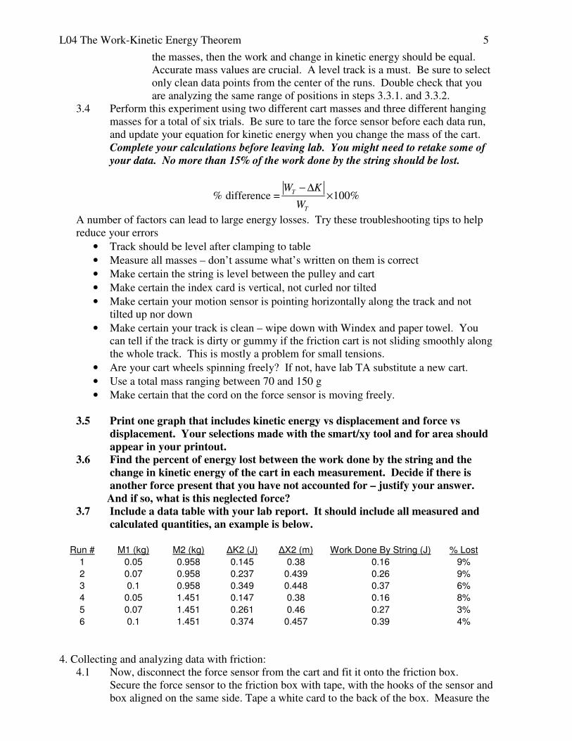
3.7 Include a data table with your lab report. It should include all measured and

calculated quantities, an example is below.

Run # M1 (kg) M2 (kg) ∆K2 (J) ∆X2 (m) Work Done By String (J) % Lost

1 0.05 0.958 0.145 0.38 0.16 9%

2 0.07 0.958 0.237 0.439 0.26 9%

3 0.1 0.958 0.349 0.448 0.37 6%

4 0.05 1.451 0.147 0.38 0.16 8%

5 0.07 1.451 0.261 0.46 0.27 3%

6 0.1 1.451 0.374 0.457 0.39 4%

4. Collecting and analyzing data with friction:

4.1 Now, disconnect the force sensor from the cart and fit it onto the friction box.

Secure the force sensor to the friction box with tape, with the hooks of the sensor and

box aligned on the same side. Tape a white card to the back of the box. Measure the

L04 The Work-Kinetic Energy Theorem 6

mass of the sensor-box assembly. Attach the string to the hook on the friction box as

you did before.

Perform the same experiment you did in section 3, being sure to update the mass in

your kinetic energy equation. Note that because there is another non-conservative

force present, the work done by the tension in the string and the change in kinetic

energy will not be equal.

4.2 Calculate the work done by the non-conservative force. Show an example of

your calculation in the report

4.3 Calculate the value of the non-conservative force. Show an example of your

calculation in the report.

4.4 Calculate the coefficient of kinetic friction, show an example of your calculation

in the report. Record these values in a chart, see table below for an example.

4.5 Print one graph that includes kinetic energy vs displacement and force vs

displacement. Your selections made with the smart/xy tool and for area should

appear in your printout.

4.6 Is your calculated value for the coefficient of friction the same for all runs?

Should it be? Where might there have been error in your experiment?

4.7 Hand in a table like the example below, as well as a table for your experiment

without friction, a sample graph from both experiments, and answers to any

bold-faced questions.

Sample Table for Experiment With Friction:

Run # M1 (kg) M2 (kg) ∆K2 (J) ∆X2 (m) Work Done By String (J) % Lost Wf = ∆K - WT

Ff =Wf / (∆x2cos180) µ = Ff/m2g

1 0.05 0.42 0 0 0 100% 0 n/a n/a

2 0.07 0.42 0.021 0.162 0.65 97% -0.629 3.883 0.942

3 0.1 0.42 0.183 0.221 0.86 78% -0.677 3.063 0.743