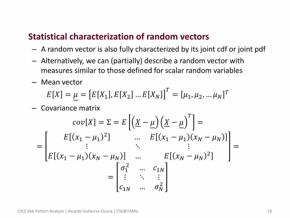
L2: Review of probability and statistics - Texas A&M...

CSCE 666 Pattern Analysis | Ricardo Gutierrez-Osuna | CSE@TAMU 1

L2: Review of probability and statistics

• Probability

– Definition of probability

– Axioms and properties

– Conditional probability

– Bayes theorem

• Random variables

– Definition of a random variable

– Cumulative distribution function

– Probability density function

– Statistical characterization of random variables

• Random vectors

– Mean vector

– Covariance matrix

• The Gaussian random variable


Review of probability theory

• Definitions (informal) – Probabilities are numbers assigned to events that

indicate “how likely” it is that the event will occur when a random experiment is performed

– A probability law for a random experiment is a rule that assigns probabilities to the events in the experiment

– The sample space S of a random experiment is the set of all possible outcomes

• Axioms of probability – Axiom I: 𝑃 𝐴𝑖 ≥ 0

– Axiom II: 𝑃 𝑆 = 1

– Axiom III: 𝐴𝑖 ∩ 𝐴𝑗 = ∅ ⇒ 𝑃 𝐴𝑖⋃𝐴𝑗 = 𝑃 𝐴𝑖 + 𝑃 𝐴𝑗

A1

A2

A3 A4

event

pro

bab

ility

A1 A2 A3 A4

Sample space

Probability law


• Warm-up exercise – I show you three colored cards

• One BLUE on both sides • One RED on both sides • One BLUE on one side, RED on the other

– I shuffle the three cards, then pick one and show you one side only. The side visible to you is RED • Obviously, the card has to be either A or C, right?

– I am willing to bet $1 that the other side of the card has the same color, and need someone in class to bet another $1 that it is the other color • On the average we will end up even, right? • Let’s try it!

A B C


• More properties of probability

– 𝑃 𝐴𝐶 = 1 − 𝑃 𝐴

– 𝑃 𝐴 ≤ 1

– 𝑃 ∅ = 0

– 𝑔𝑖𝑣𝑒𝑛 𝐴1…𝐴𝑁 , 𝐴𝑖 ∩ 𝐴𝑗 = ∅,∀𝑖𝑗 ⇒ 𝑃 ⋃ 𝐴𝑘𝑁𝑘=1 = 𝑃 𝐴𝑘

𝑁𝑘=1

– 𝑃 𝐴1⋃𝐴2 = 𝑃 𝐴1 + 𝑃 𝐴2 − 𝑃 𝐴1 ∩ 𝐴2

– 𝑃 ⋃ 𝐴𝑘𝑁𝑘=1 =

𝑃 𝐴𝑘 − 𝑃 𝐴𝑗 ∩ 𝐴𝑘 +⋯+ −1 𝑁+1𝑃 𝐴1 ∩ 𝐴2 …∩ 𝐴𝑁𝑁𝑗<𝑘

𝑁𝑘=1

– 𝐴1 ⊂ 𝐴2 ⇒ 𝑃 𝐴1 ≤ 𝑃 𝐴2


• Conditional probability – If A and B are two events, the probability of event A when we already

know that event B has occurred is

𝑃 𝐴|𝐵 =𝑃 𝐴⋂𝐵

𝑃 𝐵 𝑖𝑓 𝑃 𝐵 > 0

• This conditional probability P[A|B] is read: – the “conditional probability of A conditioned on B”, or simply

– the “probability of A given B”

– Interpretation • The new evidence “B has occurred” has the following effects

• The original sample space S (the square) becomes B (the rightmost circle)

• The event A becomes AB

• P[B] simply re-normalizes the probability of events that occur jointly with B

S S

A AB B A AB B B has

occurred


• Theorem of total probability – Let 𝐵1, 𝐵2…𝐵𝑁 be a partition of 𝑆 (mutually exclusive that add to 𝑆)

– Any event 𝐴 can be represented as

𝐴 = 𝐴 ∩ 𝑆 = 𝐴 ∩ 𝐵1 ∪ 𝐵2…𝐵𝑁 = 𝐴 ∩ 𝐵1 ∪ 𝐴 ∩ 𝐵2 … 𝐴 ∩ 𝐵𝑁

– Since 𝐵1, 𝐵2…𝐵𝑁 are mutually exclusive, then

𝑃 𝐴 = 𝑃 𝐴 ∩ 𝐵1 + 𝑃 𝐴 ∩ 𝐵2 +⋯+ 𝑃 𝐴 ∩ 𝐵𝑁

– and, therefore

𝑃 𝐴 = 𝑃 𝐴|𝐵1 𝑃 𝐵1 +⋯𝑃 𝐴|𝐵𝑁 𝑃 𝐵𝑁 = 𝑃 𝐴|𝐵𝑘 𝑃 𝐵𝑘𝑁𝑘=1

B1

B2

B3 BN-1

BN

A

B4


• Bayes theorem – Assume 𝐵1, 𝐵2…𝐵𝑁 is a partition of S

– Suppose that event 𝐴 occurs

– What is the probability of event 𝐵𝑗?

– Using the definition of conditional probability and the Theorem of total probability we obtain

𝑃 𝐵𝑗|𝐴 =𝑃 𝐴 ∩ 𝐵𝑗

𝑃 𝐴=

𝑃 𝐴|𝐵𝑗 𝑃 𝐵𝑗

𝑃 𝐴|𝐵𝑘 𝑃 𝐵𝑘𝑁𝑘=1

– This is known as Bayes Theorem or Bayes Rule, and is (one of) the most useful relations in probability and statistics


• Bayes theorem and statistical pattern recognition – When used for pattern classification, BT is generally expressed as

𝑃 𝜔𝑗|𝑥 =𝑝 𝑥|𝜔𝑗 𝑃 𝜔𝑗

𝑝 𝑥|𝜔𝑘 𝑃 𝜔𝑘𝑁𝑘=1

=𝑝 𝑥|𝜔𝑗 𝑃 𝜔𝑗

𝑝 𝑥

• where 𝜔𝑗 is the 𝑗-th class (e.g., phoneme) and 𝑥 is the

feature/observation vector (e.g., vector of MFCCs)

– A typical decision rule is to choose class 𝜔𝑗 with highest P 𝜔𝑗|𝑥

• Intuitively, we choose the class that is more “likely” given observation 𝑥

– Each term in the Bayes Theorem has a special name

• 𝑃 𝜔𝑗 prior probability (of class 𝜔𝑗)

• 𝑃 𝜔𝑗|𝑥 posterior probability (of class 𝜔𝑗 given the observation 𝑥)

• 𝑝 𝑥|𝜔𝑗 likelihood (probability of observation 𝑥 given class 𝜔𝑗)

• 𝑝 𝑥 normalization constant (does not affect the decision)


• Example – Consider a clinical problem where we need to decide if a patient has a

particular medical condition on the basis of an imperfect test

• Someone with the condition may go undetected (false-negative)

• Someone free of the condition may yield a positive result (false-positive)

– Nomenclature

• The true-negative rate P(NEG|¬COND) of a test is called its SPECIFICITY

• The true-positive rate P(POS|COND) of a test is called its SENSITIVITY

– Problem

• Assume a population of 10,000 with a 1% prevalence for the condition

• Assume that we design a test with 98% specificity and 90% sensitivity

• Assume you take the test, and the result comes out POSITIVE

• What is the probability that you have the condition?

– Solution • Fill in the joint frequency table next slide, or

• Apply Bayes rule


TEST IS POSITIVE

TEST IS NEGATIVE

ROW TOTAL

HAS CONDITION True-positive P(POS|COND)

100×0.90

False-negative P(NEG|COND) 100×(1-0.90)

100

FREE OF CONDITION

False-positive P(POS|¬COND) 9,900×(1-0.98)

True-negative P(NEG|¬COND)

9,900×0.98

9,900 COLUMN TOTAL 288 9,712 10,000


TEST IS POSITIVE

TEST IS NEGATIVE

ROW TOTAL

HAS CONDITION True-positive P(POS|COND)

100×0.90

False-negative P(NEG|COND) 100×(1-0.90)

100

FREE OF CONDITION

False-positive P(POS|¬COND) 9,900×(1-0.98)

True-negative P(NEG|¬COND)

9,900×0.98

9,900 COLUMN TOTAL 288 9,712 10,000


– Applying Bayes rule

𝑃 𝑐𝑜𝑛𝑑| + =

=𝑃 +|𝑐𝑜𝑛𝑑 𝑃 𝑐𝑜𝑛𝑑

𝑃 +=

=𝑃 +|𝑐𝑜𝑛𝑑 𝑃 𝑐𝑜𝑛𝑑

𝑃 +|𝑐𝑜𝑛𝑑 𝑃 𝑐𝑜𝑛𝑑 + 𝑃 +|¬𝑐𝑜𝑛𝑑 𝑃 ¬𝑐𝑜𝑛𝑑=

=0.90 × 0.01

0.90 × 0.01 + 1 − 0.98 × 0.99=

= 0.3125


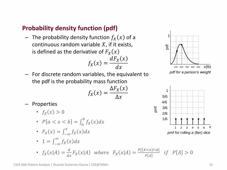
• Random variables – When we perform a random experiment we are usually interested in

some measurement or numerical attribute of the outcome • e.g., weights in a population of subjects, execution times when

benchmarking CPUs, shape parameters when performing ATR

– These examples lead to the concept of random variable • A random variable 𝑋 is a function that assigns a real number 𝑋 𝜉 to each

outcome 𝜉 in the sample space of a random experiment

• 𝑋 𝜉 maps from all possible outcomes in sample space onto the real line

– The function that assigns values to each outcome is fixed and deterministic, i.e., as in the rule “count the number of heads in three coin tosses” • Randomness in 𝑋 is due to the underlying randomness

of the outcome 𝜉 of the experiment

– Random variables can be • Discrete, e.g., the resulting number after rolling a dice

• Continuous, e.g., the weight of a sampled individual

𝝃

𝑥 = 𝑋 𝜉

𝑥

𝑆𝑥

real line

𝑆


• Cumulative distribution function (cdf) – The cumulative distribution function 𝐹𝑋 𝑥

of a random variable 𝑋 is defined as the probability of the event 𝑋 ≤ 𝑥

𝐹𝑋 𝑥 = 𝑃 𝑋 ≤ 𝑥 − ∞ < 𝑥 < ∞

– Intuitively, 𝐹𝑋 𝑏 is the long-term proportion of times when 𝑋 𝜉 ≤ 𝑏

– Properties of the cdf

• 0 ≤ 𝐹𝑋 𝑥 ≤ 1

• lim𝑥→∞

𝐹𝑋 𝑥 = 1

• lim𝑥→−∞

𝐹𝑋 𝑥 = 0

• 𝐹𝑋 𝑎 ≤ 𝐹𝑋 𝑏 𝑖𝑓 𝑎 ≤ 𝑏

• FX 𝑏 = limℎ→0

𝐹𝑋 𝑏 + ℎ = 𝐹𝑋 𝑏+

1 2 3 4 5 6

P(X

<x)

x

cdf for rolling a dice

1

5/6

4/6

3/6

2/6

1/6

P(X

<x)

100 200 300 400 500 x(lb)

cdf for a person’s weight

1


• Probability density function (pdf)

– The probability density function 𝑓𝑋 𝑥 of a continuous random variable 𝑋, if it exists, is defined as the derivative of 𝐹𝑋 𝑥

𝑓𝑋 𝑥 =𝑑𝐹𝑋 𝑥

𝑑𝑥

– For discrete random variables, the equivalent to the pdf is the probability mass function

𝑓𝑋 𝑥 =Δ𝐹𝑋 𝑥

Δ𝑥

– Properties

• 𝑓𝑋 𝑥 > 0

• 𝑃 𝑎 < 𝑥 < 𝑏 = 𝑓𝑋 𝑥 𝑑𝑥𝑏

𝑎

• 𝐹𝑋 𝑥 = 𝑓𝑋 𝑥 𝑑𝑥𝑥

−∞

• 1 = 𝑓𝑋 𝑥 𝑑𝑥∞

−∞

• 𝑓𝑋 𝑥|𝐴 =𝑑

𝑑𝑥𝐹𝑋 𝑥|𝐴 𝑤ℎ𝑒𝑟𝑒 𝐹𝑋 𝑥|𝐴 =

𝑃 𝑋<𝑥 ∩𝐴

𝑃 𝐴 𝑖𝑓 𝑃 𝐴 > 0

100 200 300 400 500

pd

f

x(lb)

pdf for a person’s weight

1

1 2 3 4 5 6

pm

f

x

pmf for rolling a (fair) dice

1

5/6

4/6

3/6

2/6

1/6


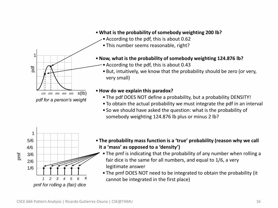
• What is the probability of somebody weighting 200 lb? • According to the pdf, this is about 0.62 • This number seems reasonable, right?

• Now, what is the probability of somebody weighting 124.876 lb?

• According to the pdf, this is about 0.43 • But, intuitively, we know that the probability should be zero (or very,

very small)

• How do we explain this paradox? • The pdf DOES NOT define a probability, but a probability DENSITY! • To obtain the actual probability we must integrate the pdf in an interval • So we should have asked the question: what is the probability of

somebody weighting 124.876 lb plus or minus 2 lb?

1 2 3 4 5 6

pm

f

x

pmf for rolling a (fair) dice

1

5/6

4/6

3/6

2/6

1/6

100 200 300 400 500

pd

f

x(lb)

pdf for a person’s weight

1

• The probability mass function is a ‘true’ probability (reason why we call it a ‘mass’ as opposed to a ‘density’)

• The pmf is indicating that the probability of any number when rolling a fair dice is the same for all numbers, and equal to 1/6, a very legitimate answer

• The pmf DOES NOT need to be integrated to obtain the probability (it cannot be integrated in the first place)


• Statistical characterization of random variables – The cdf or the pdf are SUFFICIENT to fully characterize a r.v.

– However, a r.v. can be PARTIALLY characterized with other measures

– Expectation (center of mass of a density)

𝐸 𝑋 = 𝜇 = 𝑥𝑓𝑋 𝑥 𝑑𝑥∞

−∞

– Variance (spread about the mean)

𝑣𝑎𝑟 𝑋 = 𝜎2 = 𝐸 𝑋 − 𝐸 𝑋 2 = 𝑥 − 𝜇 2𝑓𝑋 𝑥 𝑑𝑥∞

−∞

– Standard deviation 𝑠𝑡𝑑 𝑋 = 𝜎 = 𝑣𝑎𝑟 𝑋 1/2

– N-th moment

𝐸 𝑋𝑁 = 𝑥𝑁𝑓𝑋 𝑥 𝑑𝑥∞

−∞


• Random vectors

– An extension of the concept of a random variable

• A random vector 𝑋 is a function that assigns a vector of real numbers to each outcome 𝜉 in sample space 𝑆

• We generally denote a random vector by a column vector

– The notions of cdf and pdf are replaced by ‘joint cdf’ and ‘joint pdf’

• Given random vector 𝑋 = 𝑥1, 𝑥2…𝑥𝑁𝑇we define the joint cdf as

𝐹𝑋 𝑥 = 𝑃𝑋 𝑋1 ≤ 𝑥1 ∩ 𝑋2 ≤ 𝑥2 … 𝑋𝑁 ≤ 𝑥𝑁

• and the joint pdf as

𝑓𝑋 𝑥 =𝜕𝑁𝐹𝑋 𝑥

𝜕𝑥1𝜕𝑥2…𝜕𝑥𝑁

– The term marginal pdf is used to represent the pdf of a subset of all the random vector dimensions

• A marginal pdf is obtained by integrating out variables that are of no interest

• e.g., for a 2D random vector 𝑋 = 𝑥1, 𝑥2𝑇, the marginal pdf of 𝑥1 is

𝑓𝑋1 𝑥1 = 𝑓𝑋1𝑋2 𝑥1𝑥2 𝑑𝑥2

𝑥2=+∞

𝑥2=−∞


• Statistical characterization of random vectors – A random vector is also fully characterized by its joint cdf or joint pdf

– Alternatively, we can (partially) describe a random vector with measures similar to those defined for scalar random variables

– Mean vector

𝐸 𝑋 = 𝜇 = 𝐸 𝑋1 , 𝐸 𝑋2 …𝐸 𝑋𝑁𝑇= 𝜇1, 𝜇2, … 𝜇𝑁

𝑇

– Covariance matrix

𝑐𝑜𝑣 𝑋 = Σ = 𝐸 𝑋 − 𝜇 𝑋 − 𝜇𝑇=

=𝐸 𝑥1 − 𝜇1

2 … 𝐸 𝑥1 − 𝜇1 𝑥𝑁 − 𝜇𝑁⋮ ⋱ ⋮

𝐸 𝑥1 − 𝜇1 𝑥𝑁 − 𝜇𝑁 … 𝐸 𝑥𝑁 − 𝜇𝑁2

=

=𝜎12 … 𝑐1𝑁⋮ ⋱ ⋮𝑐1𝑁 … 𝜎𝑁

2


– The covariance matrix indicates the tendency of each pair of features (dimensions in a random vector) to vary together, i.e., to co-vary*

• The covariance has several important properties

– If 𝑥𝑖 and 𝑥𝑘 tend to increase together, then 𝑐𝑖𝑘 > 0

– If 𝑥𝑖 tends to decrease when 𝑥𝑘 increases, then 𝑐𝑖𝑘 < 0

– If 𝑥𝑖 and 𝑥𝑘 are uncorrelated, then 𝑐𝑖𝑘 = 0

– 𝑐𝑖𝑘 ≤ 𝜎1𝜎𝑘, where 𝜎𝑖 is the standard deviation of 𝑥𝑖

– 𝑐𝑖𝑖 = 𝜎𝑖2 = 𝑣𝑎𝑟 𝑥𝑖

• The covariance terms can be expressed as 𝑐𝑖𝑖 = 𝜎𝑖2 and 𝑐𝑖𝑘 = 𝜌𝑖𝑘𝜎𝑖𝜎𝑘

– where 𝜌𝑖𝑘 is called the correlation coefficient

Xi

Xk

Cik=-sisk

rik=-1

Xi

Xk

Cik=-½sisk

rik=-½

Xi

Xk

Cik=0

rik=0

Xi

Xk

Cik=+½sisk

rik=+½

Xi

Xk

Cik=sisk

rik=+1


A numerical example

• Given the following samples from a 3D distribution – Compute the covariance matrix

– Generate scatter plots for every pair of vars.

– Can you observe any relationships between the covariance and the scatter plots?

– You may work your solution in the templates below

Exam

ple

x 1

x 2

x 3

x 1-

1

x 2-

2

x 3-

3

(x1-

1)2

(x2-

2) 2

(x3-

3)2

(x1-

1)(

x2-

2)

(x1-

1)(

x3-

3)

(x2-

2)(

x3-

3)

1 2 3 4

Average

Variables (or features)

Examples x1 x2 x3

1 2 2 4

2 3 4 6

3 5 4 2

4 6 6 4

x1

x2

x3

x2

x3

x1


• The Normal or Gaussian distribution – The multivariate Normal distribution 𝑁 𝜇, Σ is defined as

𝑓𝑋 𝑥 =1

2𝜋 𝑛/2 Σ 1/2𝑒−12 𝑥−𝜇

𝑇Σ−1 𝑥−𝜇

– For a single dimension, this expression is reduced to

𝑓𝑋 𝑥 =1

2𝜋𝜎𝑒−𝑥−𝜇 2

2𝜎2


– Gaussian distributions are very popular since

• Parameters 𝜇, Σ uniquely characterize the normal distribution

• If all variables 𝑥𝑖 are uncorrelated 𝐸 𝑥𝑖𝑥𝑘 = 𝐸 𝑥𝑖 𝐸 𝑥𝑘 , then

– Variables are also independent 𝑃 𝑥𝑖𝑥𝑘 = 𝑃 𝑥𝑖 𝑃 𝑥𝑘 , and

– Σ is diagonal, with the individual variances in the main diagonal

• Central Limit Theorem (next slide)

• The marginal and conditional densities are also Gaussian

• Any linear transformation of any 𝑁 jointly Gaussian rv’s results in 𝑁 rv’s that are also Gaussian

– For 𝑋 = 𝑋1𝑋2…𝑋𝑁𝑇jointly Gaussian, and 𝐴𝑁×𝑁 invertible, then 𝑌 = 𝐴𝑋 is

also jointly Gaussian

𝑓𝑌 𝑦 =𝑓𝑋 𝐴

−1𝑦

𝐴


• Central Limit Theorem – Given any distribution with a mean 𝜇 and variance 𝜎2, the sampling

distribution of the mean approaches a normal distribution with mean 𝜇 and variance 𝜎2/𝑁 as the sample size 𝑁 increases • No matter what the shape of the original distribution is, the sampling

distribution of the mean approaches a normal distribution

• 𝑁 is the sample size used to compute the mean, not the overall number of samples in the data

– Example: 500 experiments are performed using a uniform distribution

• 𝑁 = 1 – One sample is drawn from the distribution

and its mean is recorded (500 times)

– The histogram resembles a uniform distribution, as one would expect

• 𝑁 = 4 – Four samples are drawn and the mean of the

four samples is recorded (500 times)

– The histogram starts to look more Gaussian

• As 𝑁 grows, the shape of the histograms resembles a Normal distribution more closely

Date post:	20-Apr-2018
Category:	Documents
Upload:	ngonhi
View:	217 times
Download:	3 times

L2: Review of probability and statistics - Texas A&M...

Documents