L211 Series Resonance and TimeFrequency Response of Passive Networks.pdf

L211 Series Resonance and Time/Frequency Response of Passive Networks

-1-

1. Abstract

In this experiment, the characteristics of series resonance RLC circuit are studied.

Resonance occurs at the point when inductor voltage and capacitor voltage are same

and at the same time, current in the circuit reaches its maximum. The relationship

between half-power frequencies, bandwidth, quality factor and selectivity are also

studied in the experiment by comparing the difference of High-Q series and Low-Q

series resonance circuit.

The time response and frequency response of RC circuit are also discussed. The

importance of time constant (τ) is studied in part B. Time constant will determine the

shape of the time response of the RC circuit. Reducing the value of τ (i.e. reducing R

or C) means that the output will change faster and that any given voltage will be

reached sooner. In terms of frequency response, the output voltage will differ with

respect to the change of the input frequency and RC circuit will act as low pass filter.

2.


-2-

1. Content

1. Abstract ................................................................................ Error! Bookmark not defined.

2. Content ........................................................................................................................................... 2

3. Introduction .................................................................................... Error! Bookmark not defined.

4. Objectives ..................................................................................................................................... 4

5. Equipment and Component ........................................................... Error! Bookmark not defined.

6. Procedure ...................................................................................................................................... 5

6.1 Low-Q and High-Q series resonance circuit ........................................................................... 5

6.2 Time/Frequency response of RC networks ............................................................................. 6

7. Results and discussion(log sheet questions) ............................................................................. 8

8. Conclusion .................................................................................................................................. 19

9. Referance ..................................................................................................................................... 20

10. Appendix ..................................................................................................................................... 21


-3-

3. Introduction:

I. Resonant circuit

Resonance in AC circuits implies a special frequency determined by the values of

the resistance, capacitance, and inductance. For series resonance the condition of

resonance is straightforward and it occurs when the inductive and capacitive

reactances are equal in magnitude but cancel each other because they are 180

degrees apart in phase. The sharp minimum in impedance which occurs is useful

in tuning applications. The sharpness of the minimum depends on the value of R

and is characterized by the quality factor "Q" of the circuit.

Resonant circuits are used to respond selectively to signals of a given frequency

while discriminating against signals of different frequencies. If the response of

the circuit is more narrowly peaked around the chosen frequency, we say that the

circuit has higher "selectivity". A "quality factor" Q, as described below, is a

measure of that selectivity, and we speak of a circuit having a "high Q" if it is

more narrowly selective.

The quality factor of a circuit is dependent upon the amount of resistance in the

circuit. The smaller the resistance, the higher the "Q" for given values of L and C.

The quality factor Q is defined by

𝑄 =𝜔0

𝛥𝜔

where Δω is the width of the resonance power curve at half maximum.

The Q is a commonly used parameter in electronics, with values usually in the

range of Q=10 to 100 for circuit applications.

II. Time/frequency response of RC networks

When we applied a dc voltage to a resistor and capacitor in series, the

capacitor charged to the applied voltage along an exponential curve, and

then just sat there. In this experiment, a square wave function is used to

study the step response of the RC circuit. Here, the input voltage will

change direction during each cycle, so the capacitor will constantly charge

and discharge as it continually tries to oppose the changes.

RC circuits, like other types of circuits, are used to "filter" a signal

waveform, changing the relative amounts of low-frequency and high-

frequency information in their output signals relative to their input signals.

There are high-pass filter and low-pass filter and band-pass filter versions.

A common application is for smoothing a signal, using a low-pass version

as discussed in this experiment.


-4-

4. Objectives

The objectives of the experiment are:

(a) To study the characteristics of series resonant circuits

(b) To investigate the step response of and RC network

(c) To study the frequency response characteristics of RC circuits

5. Equipment and components

5.1 Equipment and components for part (A)

Resisters: 47Ω ,220 Ω

Inductor: 10 mH

Capacitor: 0.1 µF

Digital Multimeter(DMM)

Function Generator

Breadboard

Digital Oscilloscope(CRO)

5.2 Equipment and components for part (B)

Resisters: 1kΩ ,100Ω

Capacitors: 0.1µF, 0.01µF

Digital multimeter(DMM)

Function generator

Breadboard

Digital oscilloscope(CRO)

d

Figure 1：Digital Multimeter(DMM) Figure 2：Function Generator

Figure 3: Breadboard Figure 4: Digital Oscilloscope (CRO)


-5-

6. Procedure:

6.1 Part(A) Low & high Q series resonance circuit

I. Low Q series resonance circuit

1) Construct the circuit of Figure 5. Measure the resistances of R and

RL(resistance of inductor). Using the nominal values of L and C and

measured resistance values, compute the radian frequency fs and quality

factor Qs of the series circuit at resonance.

2) Energize the circuit and vary the function generator from 1 kHz to 9 kHz.

One of the frequencies must be set at the resonance frequency, fs. At each

frequency, reset the input to 1 V (rms) (with the circuit connected) and

measure the rms values of the voltages VC, VR and VL with the digital

multimeter (DMM). Calculate 𝐼𝑟𝑚𝑠 =𝑉𝑅 (𝑟𝑚𝑠 )

𝑅 for each frequency.

Figure 5: Series resonant circuit

II. High Q series resonance circuit

3) Replace the 220-Ω resister with resistor of 47-Ω in the circuit of figure 5.

Repeat 1) and 2) above.

4) Draw the curves of current Irms versus frequency for low and high –Q

circuits.

5) Plot VL (rms) and VC (rms) versus frequency for the two cases.

L

Function

generator R=220Ω

VR VL

INDUCTOR

C=0.1µF

VC E=1V(RMS)

(Sine wave)

10MH

RL


-6-

6.2 (Part B &C) Time/frequency response of RC networks

1) Connect an RC circuit as shown in Figure 6.

Figure 6: RC circuit

2) Apply a square waveform of the form shown in figure 7 to the input of

figure 6.

Figure 7: Square waveform

3) Sketch the observed output waveform V0(t) on the same time scale as Vi(t)

for the valued of R and C in Table 1.

Table 1: Values of R, C and τ

R C τ=RC

(i) 1kΩ 0.1µF 0.10ms

(ii) 1kΩ 0.01µF 0.01ms

(iii) 100kΩ 0.1µF 0.01ms


-7-

4) With R=1kΩ, C=0.1µF in figure 2, measure the time constant of the circuit

from the observed step response.

5) With r=1kΩ, C=0.1µF in figure 2, apply a 5-V peak to peak sinusoidal

input with various frequency to the network. Plot the magnitude of V0/Vi

against frequency (from 100Hz to 1MHz). At the same time measure and

plot the phase angle different between Vo and Vi.

6) Draw V0 curve against frequency for network of figure 2.


-8-

7. Results and Discussion

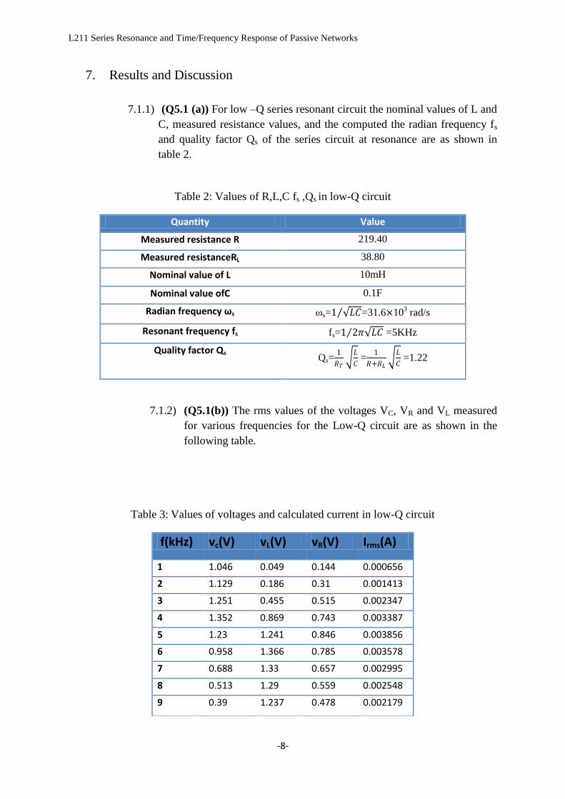
7.1.1) (Q5.1 (a)) For low –Q series resonant circuit the nominal values of L and

C, measured resistance values, and the computed the radian frequency fs

and quality factor Qs of the series circuit at resonance are as shown in

table 2.

Table 2: Values of R,L,C fs ,Qs in low-Q circuit

Quantity Value

Measured resistance R 219.40

Measured resistanceRL 38.80

Nominal value of L 10mH

Nominal value ofC 0.1F

Radian frequency ωs ωs=1 𝐿𝐶 =31.6×103 rad/s

Resonant frequency fs fs=1 2𝜋 𝐿𝐶 =5KHz

Quality factor Qs Qs=

1

𝑅𝑇 𝐿

𝐶 =

1

𝑅+𝑅𝐿 𝐿

𝐶 =1.22

7.1.2) (Q5.1(b)) The rms values of the voltages VC, VR and VL measured

for various frequencies for the Low-Q circuit are as shown in the

following table.

Table 3: Values of voltages and calculated current in low-Q circuit

f(kHz) vc(V) vL(V) vR(V) Irms(A)

1 1.046 0.049 0.144 0.000656

2 1.129 0.186 0.31 0.001413

3 1.251 0.455 0.515 0.002347

4 1.352 0.869 0.743 0.003387

5 1.23 1.241 0.846 0.003856

6 0.958 1.366 0.785 0.003578

7 0.688 1.33 0.657 0.002995

8 0.513 1.29 0.559 0.002548

9 0.39 1.237 0.478 0.002179


-9-

7.1.3) (Q5.2(a)) For High –Q series resonant circuit the nominal values of

L and C, measured resistance values, and the computed the radian

frequency fs and quality factor Qs of the series circuit at resonance

are as shown in table 4.

Table 4: Values of R,L,C fs ,Qs in high-Q circuit

Value

Measured resistance R 46.90

Measured resistanceRL 38.80

Nominal value of L 10mH

Nominal value ofC 0.1F

Radian frequency ωs ωs=1 𝐿𝐶 =31.6×103 rad/s

Resonant frequency fs fs=1 2𝜋 𝐿𝐶 =5KHz

Quality factor Qs Qs=

1

𝑅𝑇 𝐿

𝐶 =

1

𝑅+𝑅𝐿 𝐿

𝐶 =

7.1.4) (Q5.2(b)) The rms values of the voltages VC, VR and VL measured

for various frequencies for the Low-Q circuit are as shown in the

following table.

Table 5: Values of voltages and calculated current in high-Q circuit

f(kHz)) vc(V) vL(V) vR(V) Irms(A)

1 1.057 0.05 0.031 0.000661

2 1.206 0.201 0.071 0.001514

3 1.526 0.555 0.134 0.002857

4 2.39 1.545 0.279 0.005949

5 3.57 3.628 0.521 0.011109

6 1.854 2.678 0.324 0.006908

7 0.997 1.938 0.203 0.004328

8 0.645 1.625 0.15 0.003198

9 0.459 1.457 0.12 0.002559


-10-

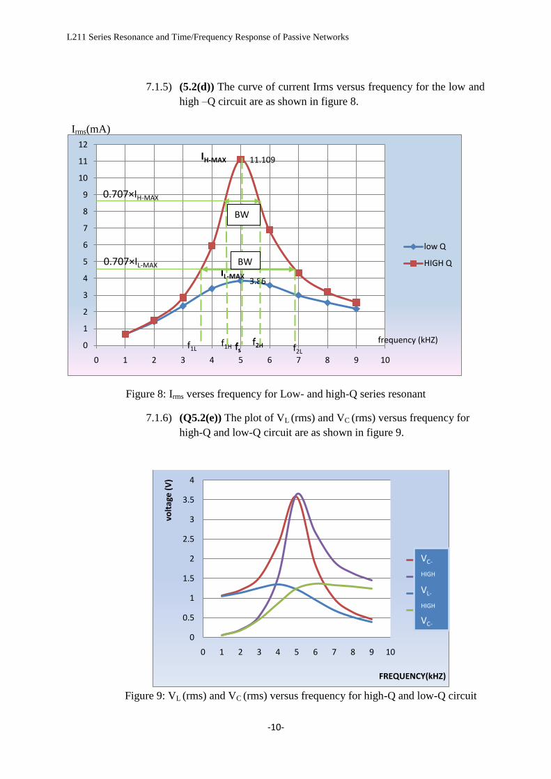
7.1.5) (5.2(d)) The curve of current Irms versus frequency for the low and

high –Q circuit are as shown in figure 8.

Figure 8: Irms verses frequency for Low- and high-Q series resonant

7.1.6) (Q5.2(e)) The plot of VL (rms) and VC (rms) versus frequency for

high-Q and low-Q circuit are as shown in figure 9.

Figure 9: VL (rms) and VC (rms) versus frequency for high-Q and low-Q circuit

3.86

11.109

0

1

2

3

4

5

6

7

8

9

10

11

12

0 1 2 3 4 5 6 7 8 9 10

low Q

HIGH Q

f1L fsf2Hfsf2Hfs

f1H f2L

IH-MAX

IL-MAX

0.707×IL-MAX

0.707×IH-MAX

frequency (kHZ)

0

0.5

1

1.5

2

2.5

3

3.5

4

0 1 2 3 4 5 6 7 8 9 10

volt

age

(V

)

FREQUENCY(kHZ)

vc

vl

vc

vL

VC-

HIGH

VL-

HIGH

VC-

BW

BW

Irms(mA)


-11-

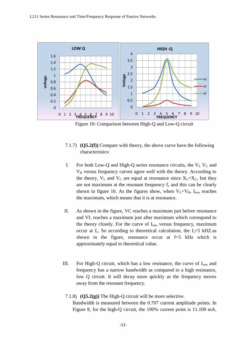
Figure 10: Comparison between High-Q and Low-Q circuit

7.1.7) (Q5.2(f)) Compare with theory, the above curve have the following

characteristics:

I. For both Low-Q and High-Q series resonance circuits, the VL VC and

VR versus frequency curves agree well with the theory. According to

the theory, VL and VC are equal at resonance since XL=XC, but they

are not maximum at the resonant frequency fs and this can be clearly

shown in figure 10. As the figures show, when VL=VR, Irms reaches

the maximum, which means that it is at resonance.

II. As shown in the figure, VC reaches a maximum just before resonance

and VL reaches a maximum just after maximum which correspond to

the theory closely. For the curve of Irms versus frequency, maximum

occur at fs. So according to theoretical calculation, the fs=5 kHZ.as

shown in the figure, resonance occur at f=5 kHz which is

approximately equal to theoretical value.

III. For High-Q circuit, which has a low resistance, the curve of Irms and

frequency has a narrow bandwidth as compared to a high resistance,

low Q circuit. It will decay more quickly as the frequency moves

away from the resonant frequency.

7.1.8) (Q5.2(g)) The High-Q circuit will be more selective.

Bandwidth is measured between the 0.707 current amplitude points. In

Figure 8, for the high-Q circuit, the 100% current point is 11.109 mA.

0

0.2

0.4

0.6

0.8

1

1.2

1.4

1.6

0 1 2 3 4 5 6 7 8 9 10

volt

age

FREQUENCY

LOW Q

0

0.5

1

1.5

2

2.5

3

3.5

4

0 1 2 3 4 5 6 7 8 9 10

Vo

ltag

e

FREQUENCY

HIGH -Q

vc

vr

vl

http://www.allaboutcircuits.com/vol_2/chpt_6/6.html#22051.png


-12-

The 70.7% level is 0707(111.109 mA)=7.85 mA. The upper and lower

band edges read from the curve are 4.4k Hz for fl-H and 5.8k Hz for f2-H.

The bandwidth is 1.4k Hz. Similarly in the figure of the Low-Q curve,

the bandwidth of low-Q circuit will be 4 kHZ. Thus, for high Q circuit,

it has smaller bandwidth.

Actually, according to theory, BW=S

S

Q

ff 12f , which means that

BW is negatively proportional to quality factor. For RLC circuit, the

smaller the BW, the higher the circuit selectivity, at the same time, it

also means that the larger Qs, the higher the circuit selectivity.

Thus, for High-Q circuit has smaller bandwidth, it will has a larger Qs

and also has a higher selectivity.

7.1.9) (Q5.2(h)(i))Using the equation Qs = |Vc|s/E ,the calculated Qs is as

shown below:

For the Low-Q circuit: Qs = |Vc|s/E = 1.23/1 =1.23

For the High-Q circuit: Qs = |Vc|s/E = 3.69/1 = 3.69

Using the equation Qs = fs/BW, the values of Qs are also as shown:

For the Low-Q circuit: Qs = fs/BW = fs/( LOWLOW f _1_2f )=5.033/(7.2-3.2) = 1.26

For the High-Q circuit: Qs = fs/BW = fs/( HIGHHIGH ff _1_2 )5.033/(4.4-5.8) = 3.60

According to the above calculation, the values of Qs for each circuit are

approximately the same. Actually, the theoretical values of the circuit are Q

223.1_ LOWS and Q 69.3_ HIGHS correspondingly and the above values

calculated almost consist with them respectively.

7.1.10) (Q5.2(j)) At frequencies below the resonant frequency, the current

leads the voltage, which is characteristic of an RC circuit. As the

power factor of the RC circuit are less than 1 and it is leading power

factor, the power factor of the circuit are pf<1 (leading).

At the resonant frequency, the voltage of the capacitor and inductor

are the same. And the impedance of the capacitor and inductor are

also the same. So the total apparent power is equal to the average


-13-

power dissipated by the resistor and the power factor is equal to 1.

This is a maximum power factor. Thus, at resonant frequency, pf=1.

At frequency above resonance, the current lags the voltage, and the

series RLC circuit looks like a series RL circuit. Thus, the power

factor at high frequency pf<1 (lagging).

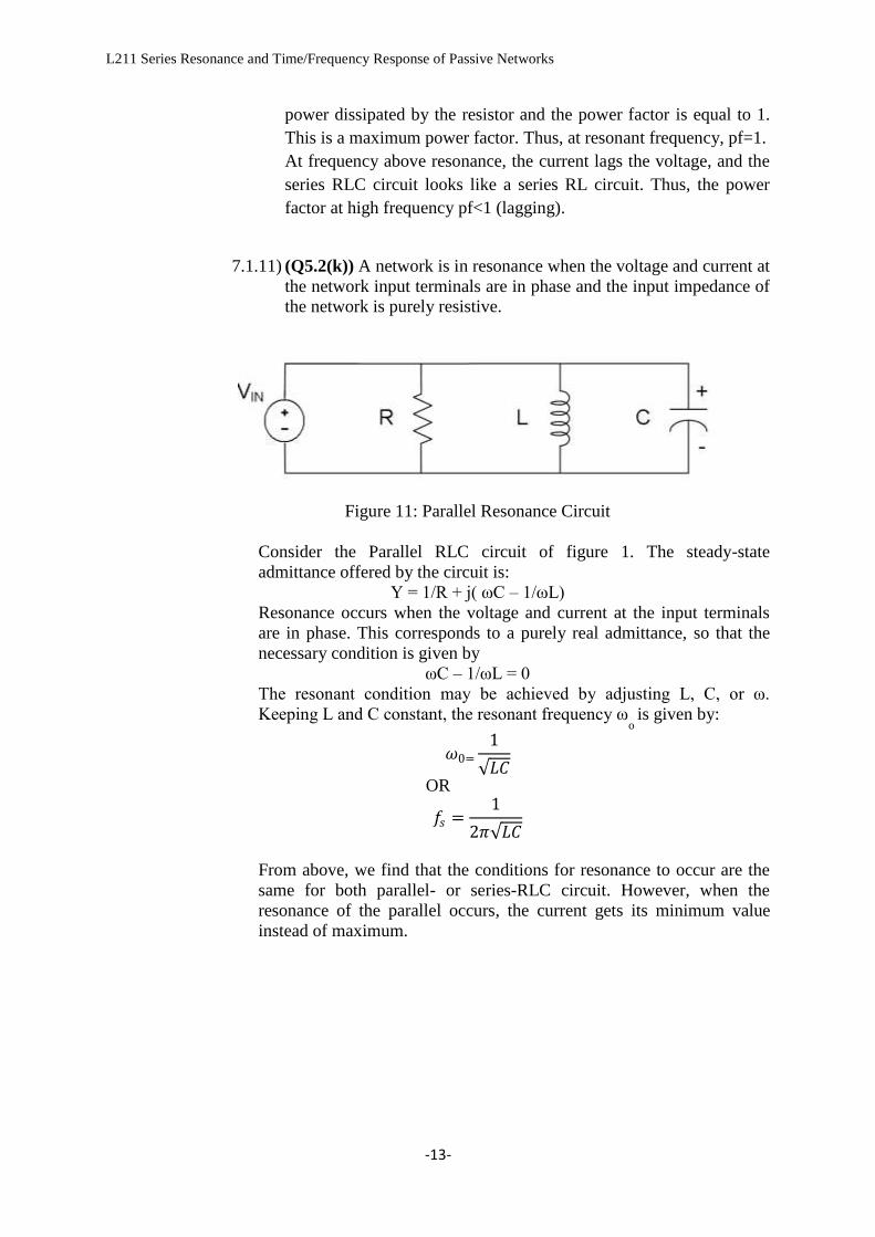
7.1.11) (Q5.2(k)) A network is in resonance when the voltage and current at

the network input terminals are in phase and the input impedance of

the network is purely resistive.

Figure 11: Parallel Resonance Circuit

Consider the Parallel RLC circuit of figure 1. The steady-state

admittance offered by the circuit is:

Y = 1/R + j( ωC – 1/ωL)

Resonance occurs when the voltage and current at the input terminals

are in phase. This corresponds to a purely real admittance, so that the

necessary condition is given by

ωC – 1/ωL = 0

The resonant condition may be achieved by adjusting L, C, or ω.

Keeping L and C constant, the resonant frequency ωo is given by:

𝜔0=

1

𝐿𝐶

OR

𝑓𝑠 =1

2𝜋 𝐿𝐶

From above, we find that the conditions for resonance to occur are the

same for both parallel- or series-RLC circuit. However, when the

resonance of the parallel occurs, the current gets its minimum value

instead of maximum.


-14-

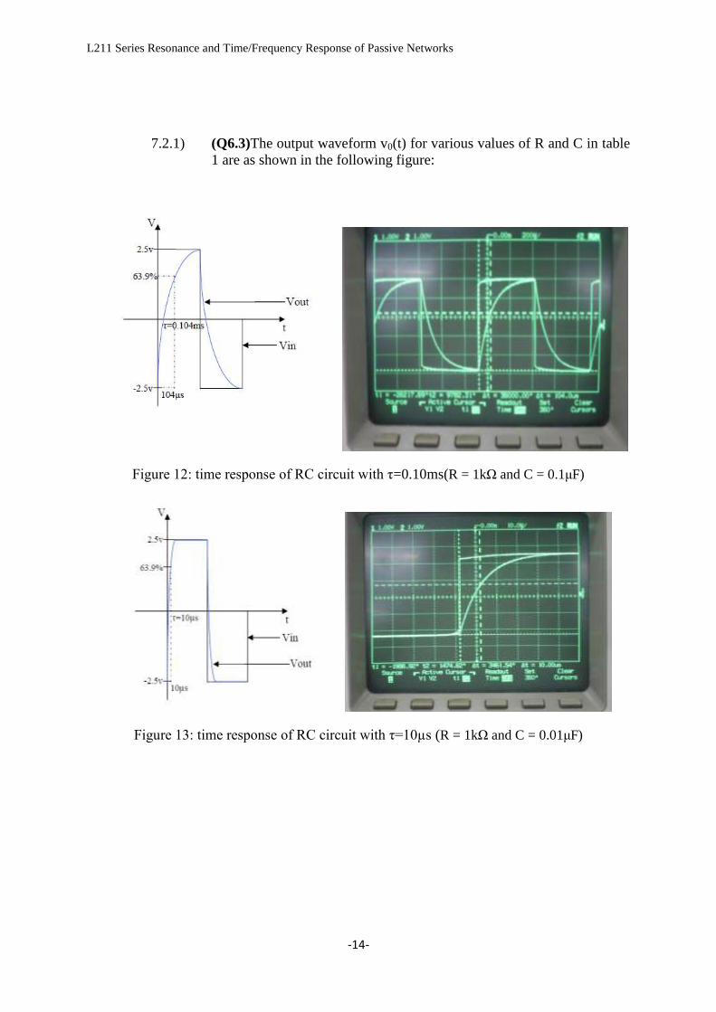
7.2.1) (Q6.3)The output waveform v0(t) for various values of R and C in table

1 are as shown in the following figure:

Figure 12: time response of RC circuit with τ=0.10ms(R = 1kΩ and C = 0.1μF)

Figure 13: time response of RC circuit with τ=10µs (R = 1kΩ and C = 0.01μF)


-15-

Figure 14: time response of RC circuit with τ=10µs (R = 100Ω and C = 0.1μF)

7.2.2) (Q6.2.1) To study the step response of RC circuit, step input should be

used. However, if only one step is used, the step response will just

occur at the time when the step input is injected into the system and it

will last a very short time. (Actually when the time exceeds five time

constants, the capacitor voltage will be nearly the same as the final

voltage.)

When a square wave is used, the capacitor will be charged and

discharged continuously during each cycle of the square wave. Each

positive and negative cycle of the square wave can be viewed as a step

function and hence the step response of the system can be studied.

7.2.3) (Q6.5) The output voltage (Vc) reaches 63.2% of its final value in 1

time constant (1 second in this case). In general, the time taken to reach

a particular value is related to the number of time constants given in the

table below.

Table 6: Number of time constants required to reach a proportion of the final value

τ 2 τ 3τ 4 τ 5 τ

63.2% 86.5% 95.0% 98.2% 99.3%


-16-

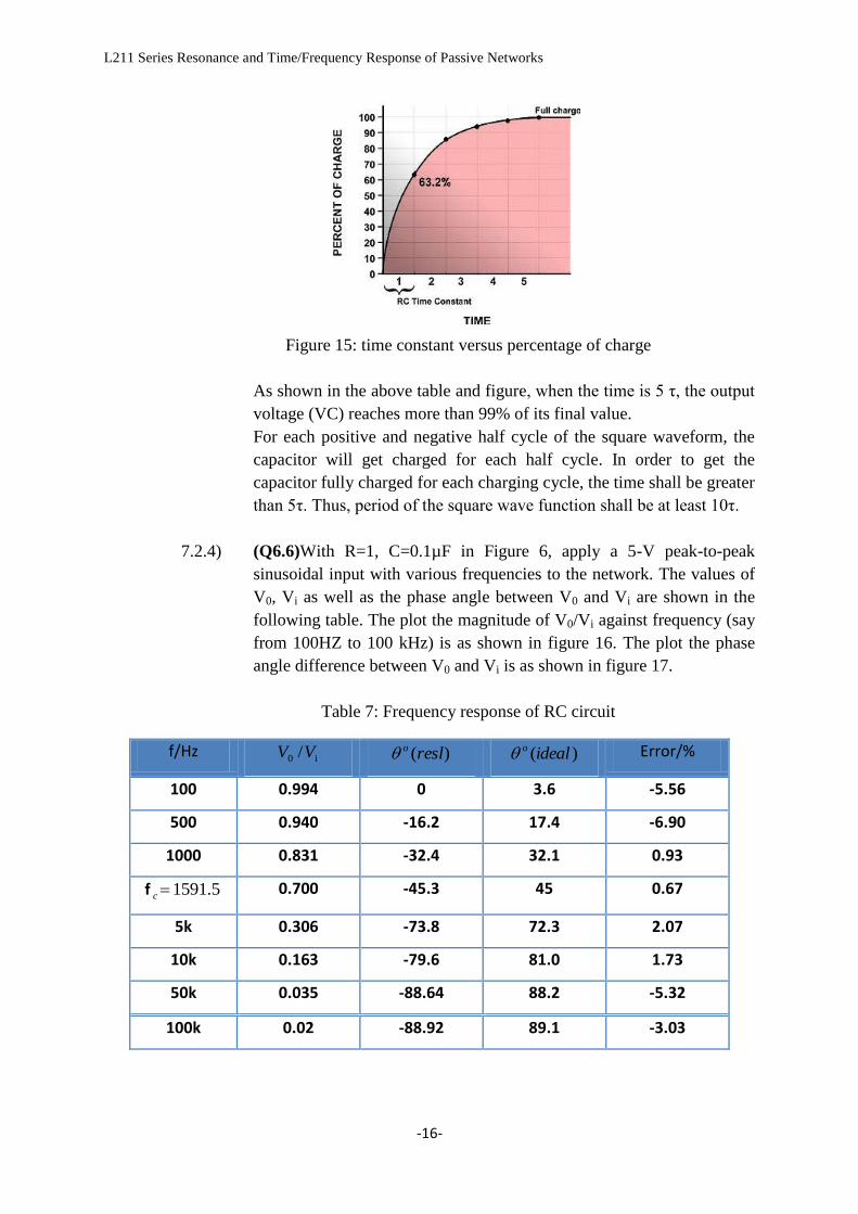
Figure 15: time constant versus percentage of charge

As shown in the above table and figure, when the time is 5 τ, the output

voltage (VC) reaches more than 99% of its final value.

For each positive and negative half cycle of the square waveform, the

capacitor will get charged for each half cycle. In order to get the

capacitor fully charged for each charging cycle, the time shall be greater

than 5τ. Thus, period of the square wave function shall be at least 10τ.

7.2.4) (Q6.6)With R=1, C=0.1µF in Figure 6, apply a 5-V peak-to-peak

sinusoidal input with various frequencies to the network. The values of

V0, Vi as well as the phase angle between V0 and Vi are shown in the

following table. The plot the magnitude of V0/Vi against frequency (say

from 100HZ to 100 kHz) is as shown in figure 16. The plot the phase

angle difference between V0 and Vi is as shown in figure 17.

Table 7: Frequency response of RC circuit

f/Hz i0 /VV )(reslo )(idealo Error/%

100 0.994 0 3.6 -5.56

500 0.940 -16.2 17.4 -6.90

1000 0.831 -32.4 32.1 0.93

f 5.1591c 0.700 -45.3 45 0.67

5k 0.306 -73.8 72.3 2.07

10k 0.163 -79.6 81.0 1.73

50k 0.035 -88.64 88.2 -5.32

100k 0.02 -88.92 89.1 -3.03


-17-

Figure 16: Plot of V0/Vi versus frequency

Figure 17: phase angle between V0 and Vi versus frequency

7.2.5) (Q6.7) V0 curve against frequency for network of figure 6 can be draw

from table 5 as i

0

i

0

o 5*V

V

V

VVV i and the value of

i

0

V

V can be got from table

5 directly. The graph is shown below:

0.9940.9376

0.8312

0.7

0.306

0.1630.035

0.02

0

0.2

0.4

0.6

0.8

1

1.2

1 10 100 1000 10000 100000

V0/

VI

frequency (Hz)

-100

-90

-80

-70

-60

-50

-40

-30

-20

-10

0

1 10 100 1000 10000 100000

ph

ase

an

gle

frequency(Hz)


-18-

Figure 18: V0 versus frequency

According to the plot and the theory, it is shown that the RC circuit in the

experiment is Low-pass filter as for low frequency the output voltage is much

higher than that at high frequency.

7.2.6) (Q6.8) Comment on phase angle of the transfer function:

According to the step 5, we know that the phase angle keeps be larger

while the transfer function keeps be larger. What’s more, the changing

rate of the phase angle and the transfer function both first become larger

and then smaller. Therefore, it is reasonable that we can assume the

relation between the phase angle and the transfer function is negatively

proportional.

0

1

2

3

4

5

6

1 10 100 1000 10000 100000

V0

frequency (Hz)

Series1


-19-

8 Conclusion:

I. For the resonance of a series RLC circuit occurs when the inductive and

capacitive reactance are equal in magnitude but cancel each other

because they are 180 degrees apart in phase. At the same time, VC=VL

and Irms reaches its maximum value.

II. The selectivity of a circuit depends on the quality factor of the circuit. As

for higher Qs, the selectivity is higher. The selectivity can also be told

from the curve of the response of the circuit. If the curve is more

narrowly peaked around some certain frequency, thus it will have a small

bandwidth and we call that the circuit has higher selectivity.

III. For the time response of a RC circuit, the shape of the curve depend

highly on the time constant of the circuit which τ=RC. Time constant can

also be got from the curve of the step response of the circuit which

equals to the time for the voltage to become 63% of its final value.

IV. The frequency response of the circuit can tell the properties of the RC

circuit. For example, the experiment show that the circuit in figure is

Low-pass circuit which means that it will give high output at low

frequency while low output at high frequency.


-20-

9 Reference

1) Paul A. Tipler, ―Physics for Scientists and Engineers‖，3rd edition，Extend version

2) R. A. Serway & J. W. Jewett, Jr. “Physics for Scientists and Engineers with Modern

Physics‖, 6th Edition,

3) Retrieved September/20/2009 http://en.wikipedia.org/wiki/RLC_circuit

4) Laboratory Experiment EE2071 Laboratory Manual for Experiment L211


-21-

10 Appendix

11

Quality Factor and Bandwidth (BW)

The quality factor sQ of a series resonant circuit is defined as the ratio of the reactive

power of either the inductor or the capacitor to the average power of the resistor at

resonance, i.e.,

sQ =C

L

RL

LCRR

Lf

R

L

RI

XI

TTT

s

T

S

T

L 1)

2

1(

22

*

*

power average

power reactive2

2

Therefore, at resonance the voltage across the inductor V L can be written as:

T

L

S

LSL

R

EX

Z

EXV

**|| EQE

R

LV S

T

sL

s||

Similarly, EQV SSC || and where R RRLT

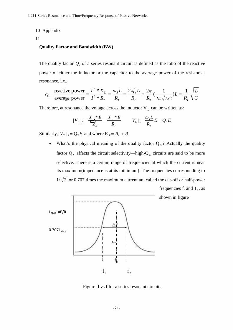
What’s the physical meaning of the quality factor Q S ? Actually the quality

factor Q S affects the circuit selectivity—high-Q S circuits are said to be more

selective. There is a certain range of frequencies at which the current is near

its maximum(impedance is at its minimum). The frequencies corresponding to

1/ 2 or 0.707 times the maximum current are called the cut-off or half-power

frequencies f 1 and 2f , as

shown in figure

Figure :I vs f for a series resonant circuits

BW

0.707I MAX

I MAX =E/R

1f 2f


-22-

The frequency range between 1f and 2f is called the bandwidth (BW) of the resonant

circuit, i.e., BW=f 2 -2f =

s

s

Q

f

The smaller the BW, the higher the circuit selectivity. For circuits where Q S >=10, the

resonant frequency sf approximately bisects the BW and the resonant curve is

symmetrical about sf .

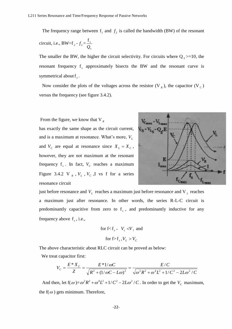
Now consider the plots of the voltages across the resistor (VR

), the capacitor (V C )

versus the frequency (see figure 3.4.2).

From the figure, we know that V R

has exactly the same shape as the circuit current,

and is a maximum at resonance. What’s more, LV

and CV are equal at resonance since CL XX ,

however, they are not maximum at the resonant

frequency sf . In fact, CV reaches a maximum

Figure 3.4.2 V R , LV , CV ,I vs f for a series

resonance circuit

just before resonance and LV reaches a maximum just before resonance and V L reaches

a maximum just after resonance. In other words, the series R-L-C circuit is

predominantly capacitive from zero to sf , and predominantly inductive for any

frequency above sf , i.e.,

for f< sf ， lVV c and

for f> sf , CL VV

The above characteristic about RLC circuit can be proved as below:

We treat capacitor first:

CLCLR

CE

LCR

CE

Z

XEV C

C

/2/1

/

)/1(

/1**

22242222

And then, let f( )= CLCLR /2/1 222422 . In order to get the CV maximum,

the f( ) gets minimum. Therefore,


-23-

0)(d

d

f LRCL // 22 LRCL // 2 < CLS / ,

Which means that SMAXC f_f .

Similarly, it is easy to prove that sL ff max_

Time constant

When a capacitor (C) is connected to a dc voltage source like a battery, charge builds

upon its plates and the voltage across the plates increases until it equals the voltage (V)

of the battery. At any time (t), the charge (Q) on the capacitor plates is given by Q =CV.

The rate of voltage rise depends on the value of the capacitance and the resistance in

the circuit. Similarly, when a capacitor is discharged, the rate of voltage decay depends

on the same parameters.

Both charging and discharging times of a capacitor are characterized by a quantity

called the time constant τ, which is the product of the capacitance (C) and the resistance

(R), i.e. τ= RC.

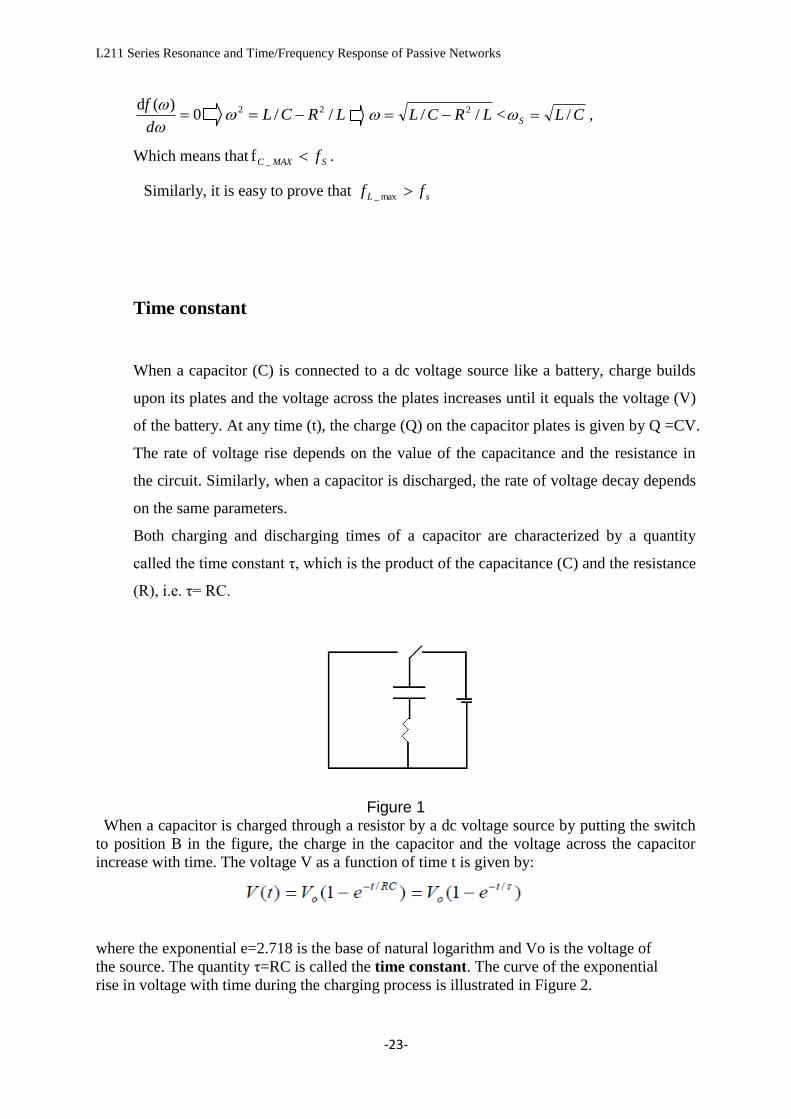
Figure 1

When a capacitor is charged through a resistor by a dc voltage source by putting the switch

to position B in the figure, the charge in the capacitor and the voltage across the capacitor

increase with time. The voltage V as a function of time t is given by:

where the exponential e=2.718 is the base of natural logarithm and Vo is the voltage of

the source. The quantity τ=RC is called the time constant. The curve of the exponential

rise in voltage with time during the charging process is illustrated in Figure 2.


-24-

At time t=τ=RC (one time constant), the voltage across the capacitor has grown to a value:

It will take an infinite amount of time for the capacitor to fully charge to its maximum

value. For practical purposes we will assume the after five time constants the capacitor is

fully charged.

When a fully charged capacitor is discharged through a resistor by putting the switch to

position A in Figure 1, the voltage across the capacitor decreases with time. The voltage

V as a function of time t is given by:

The exponential decay of the voltage with time is also illustrated in Figure 2. After a time

t=τ=RC (one time constant), the voltage across the capacitor has decreased to a value:


-25-

Similar equations for charging and discharging of the capacitor exist for the charge Q

across the plates of the capacitor. These are:

Charging

Discharging:

Date post:	28-Oct-2015
Category:	Documents
Upload:	glenlcy
View:	129 times
Download:	0 times

L211 Series Resonance and TimeFrequency Response of Passive Networks.pdf

Documents