LA-11575-T Thesis UC-4U and UC-414 Issued: May 1989 LA— 11575-T DE89 013175 Observation of the Negative Muonium Ion in Vacuum Yunan Kuang* *Craduate Research Assistant at Los Alamos. Physics Department, College of William and Mary, Williamsburg, Virginia 23185. DISTRIBUTION CF THIS DOCUMENT IS UNLIMITED Los Alamos National Laboratoi Los Alamos, New Mexico 8754 1ASTEH
Transcript
LA-11575-TThesis
UC-4U and UC-414Issued: May 1989
LA— 11575-T
DE89 013175
Observation of the Negative
Muonium Ion in Vacuum
Yunan Kuang*
*Craduate Research Assistant at Los Alamos.Physics Department, College of William and Mary, Williamsburg, Virginia 23185.
DISTRIBUTION CF THIS DOCUMENT IS UNLIMITED
Los Alamos National LaboratoiLos Alamos, New Mexico 87541ASTEH
Contents
List of Figures iii
List of Tables viii
Acknowledgements xi
Abstract xii
1 Introduction 1
2 Physical Principles 4
2.1 Properties of the Negative Muonium Ion and Muon Decay 42.2 Charge Capture Processes 72.3 Subsurface Positive Muon Beam 11
3 Experimental Technique and Apparatus 133.1 Separated Subsurface Beam of Positive Muons 16
3.2 Production Foil 20
3.3 Accelerator 21
3.4 Magnetic Spectrometer 23
3.5 Solenoid 23
3.6 Transport System 28
3.7 Detectors and Logic 30
4 Experimental Observations 43
v
4.1 Observation of Muonium Formation 43
4.2 Studies of Low Energy Positive Muons 48
4.3 Observation of the Formation of the Negative Muonium Ion 58
5 Data Analysis 64
5.1 The Michel Spectrum 64
5.2 Muon Lifetime 69
5.3 The Time-of-Flight Spectrum 71
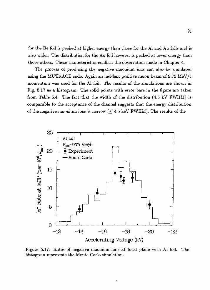
5.4 Rates of the Low Energy Positive Muons and the Negative Muonium
Ions 82
5.5 Monte Carlo Simulations 86
6 Summary and Discussion 98
A MUTRACE 101
A.I Introduction 101
A.2 Energy Loss and Range of Positive Muons 102
A.3 Multiple Scattering 103
A.4 Charge Exchange 106
A.5 Transport of Charged Particles 106
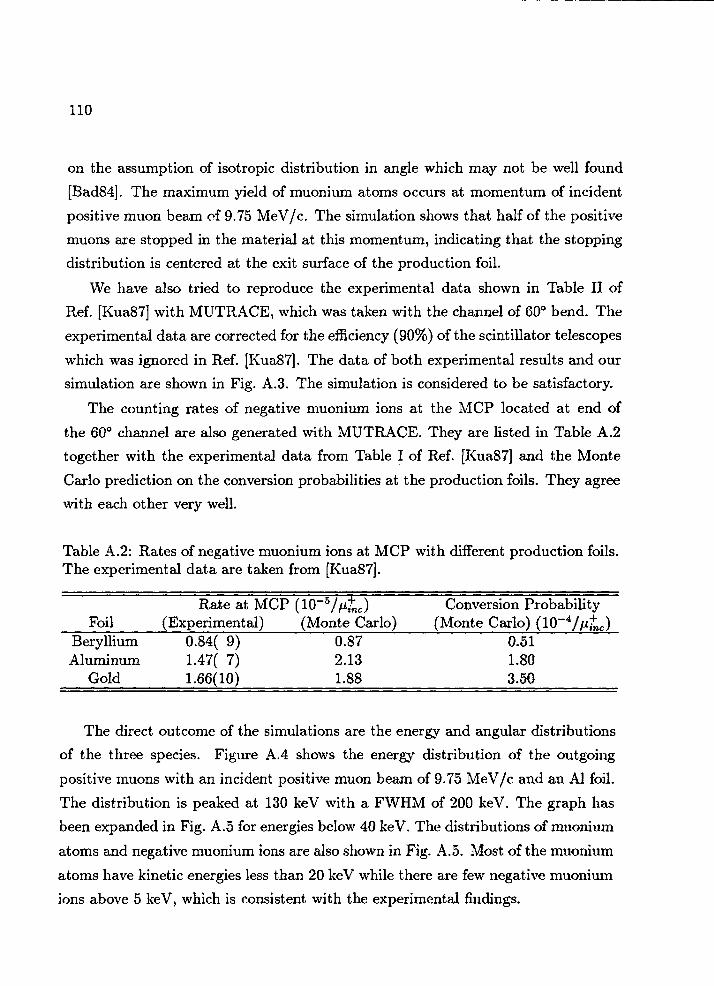
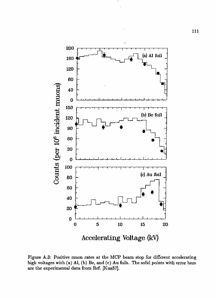
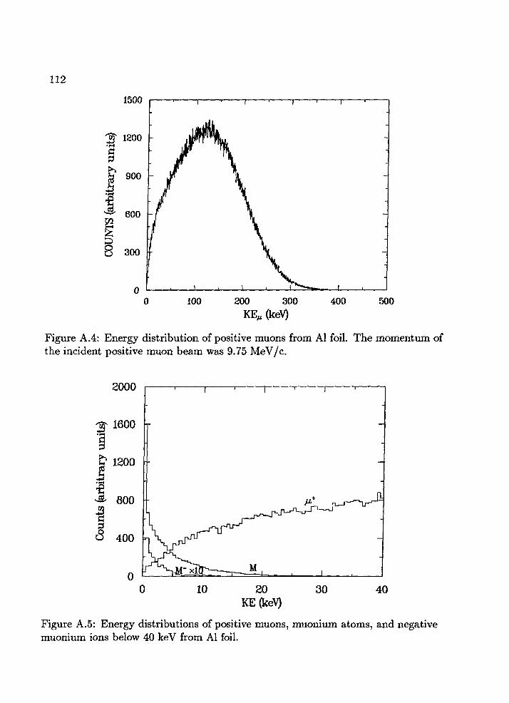
A.6 Application to the Experimental Data 108
A.7 Conclusion 115
A.8 Acknowledgement 115
Bibliography 116
B First observation of the negative muonium ion produced by elec-
tron capture in a beam-foil experiment 123
v i
List of Figures
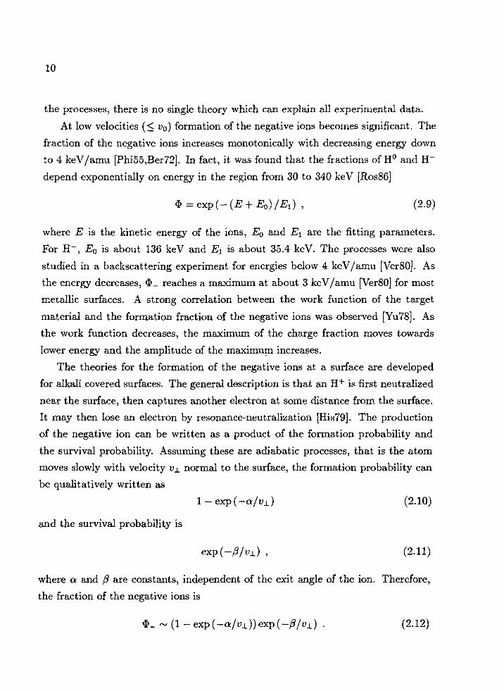
2.1 Lowest energy levels of H based on [Bur68] 5
2.2 Charge fractions of emerging muonium ions 9
3.1 Schematic diagram of the experimental apparatus for observation of
the charge states of the outgoing beams when positive muons pass
through a thin foil. The insert in the lower left corner is an enlarged
view of the accelerator 14
3.2 The horizontal view of the detector arrangement at the end of the
60° channel 15
3.3 Layout of the stopped muon channel (SMC). The present experiment
was carried out in the west cave (CAVE A) 17
3.4 Layout of the channel extension which connects the stopped muon
channel (SMC) to the experimental apparatus 18
3.5 Electrostatic accelerator and the equipotential lines computed using
POISSON group programs 22
3.6 Momentum acceptance of the solenoid based on MUTRACE calcu-
lation. l0 = 40 cm, /, = 25 cm, 3 = 713 G, I = 135 cm 26
3.7 Magnetic field along the axis of the solenoid. The solid points with
error bars represent the measurement, while the curve is based on
POISSON calculation 28
3.8 Beam envelope of the transport system 29
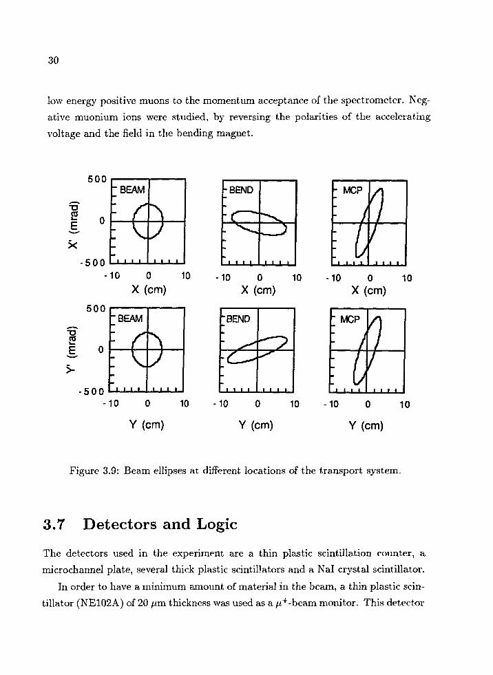
3.9 Beam ellipses at different locations of the transport system 30
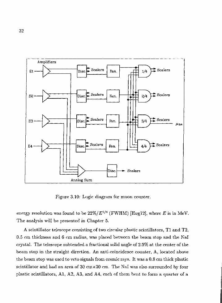
3.10 Logic diagram for muon counter 32
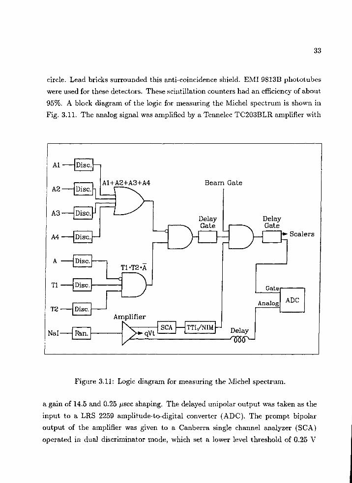
3.11 Logic diagram for measuring the Michel spectrum 33
vii
3.12 Schematic diagram of the wiring for the MCP detector 35
3.13 Logic diagram of the scintillator telescopes for detecting decay posi-
trons from MCP 36
3.14 Logic diagram for muon lifetime and time-of-flight measurements. . . 37
3.15 Circuit diagram for calibrating TDC's 38
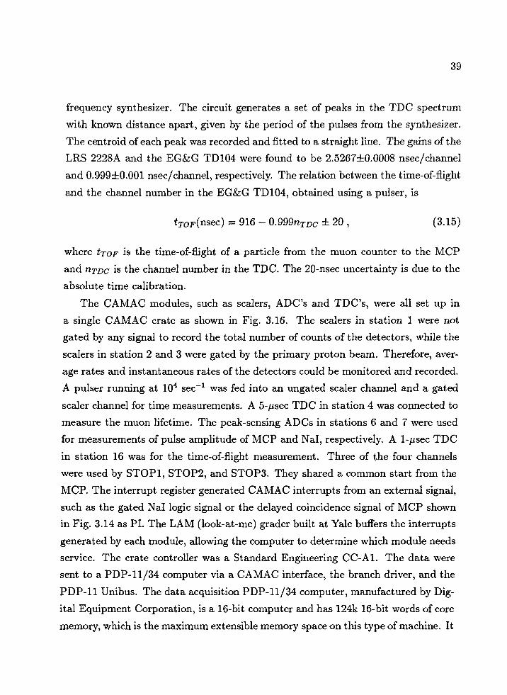
3.16 CAMAC module arrangement in the crate 40
4.1 ADC spectrum of the Nal detector taken when the field in the bend-
ing magnet was switched off. 44
4.2 ADC spectrum of the Nal detector taken when the fields in the bend-
ing magnet and the separator were turned off. 45
4.3 ADC spectrum of the Nal detector taken when the field in the bend-
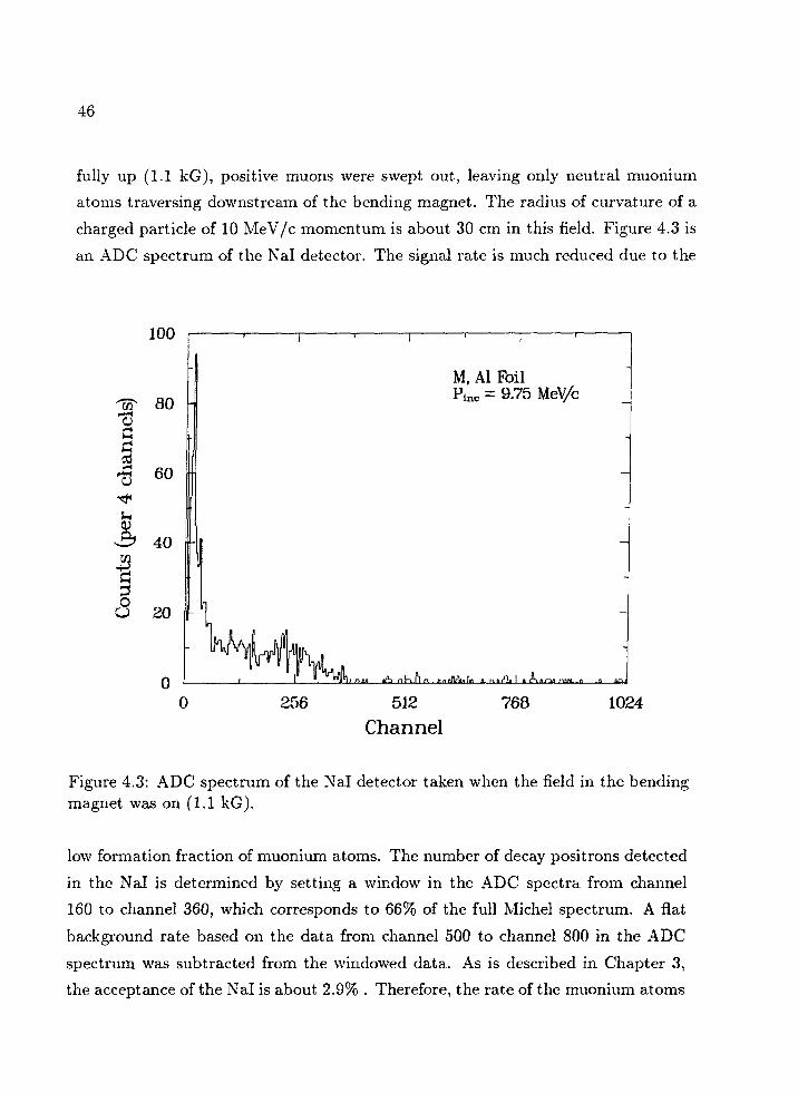
ing magnet was on (1.1 kG) 46
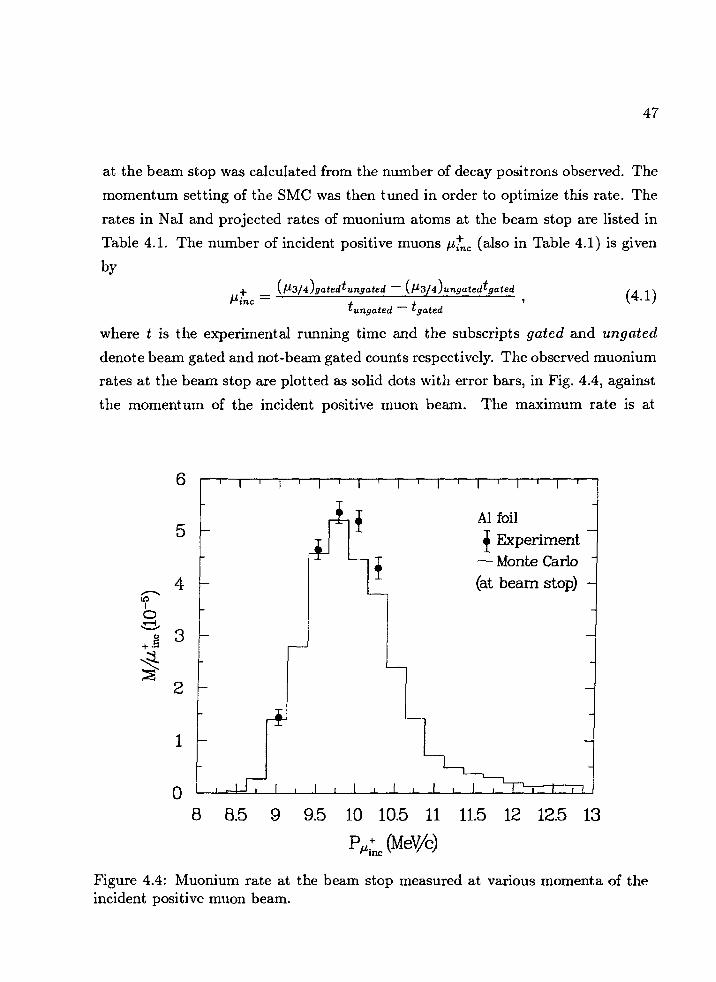
4.4 Muonium rate at the beam stop measured at various momenta of the
incident positive muon beam 47
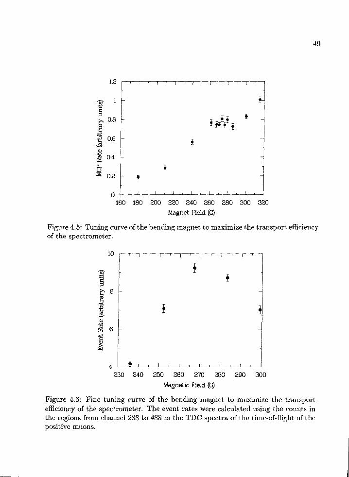
4.5 Tuning curve of the bending magnet to maximize the transport effi-
ciency of the spectrometer 49
4.6 Fine tuning curve of the bending magnet to maximize the transport
efficiency of the spectrometer. The event rates were calculated using
the counts in the regions from channel 288 to 488 in the TDC spectra
of the time-of-flight of the positive muons 49
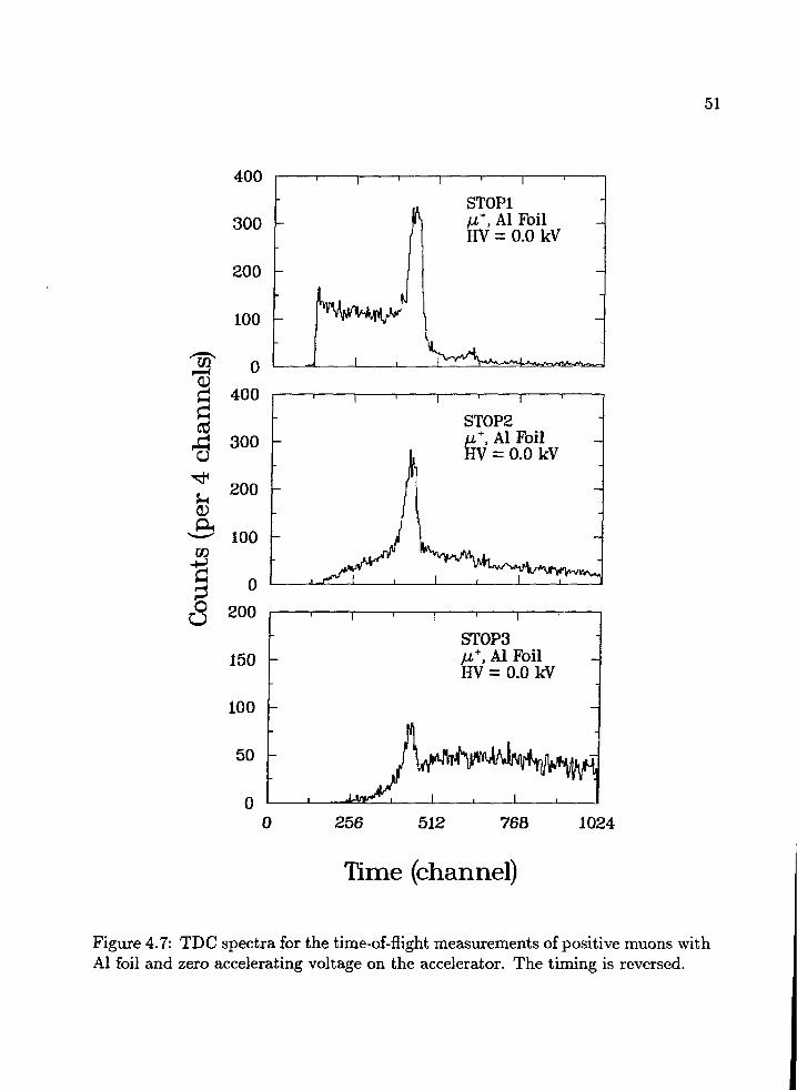
4.7 TDC spectra for the time-of-flight measurements of positive muons
with Al foil and zero accelerating voltage on the accelerator. The
timing is reversed 51
4.8 TDC spectra for the time-of-flight measurements of positive muons
with Al foil and accelerating voltage of 19 kV on the accelerator. The
timing is again reversed 52
4.9 TDC spectrum for the lifetime measurements of positive muons with
Al foil 55
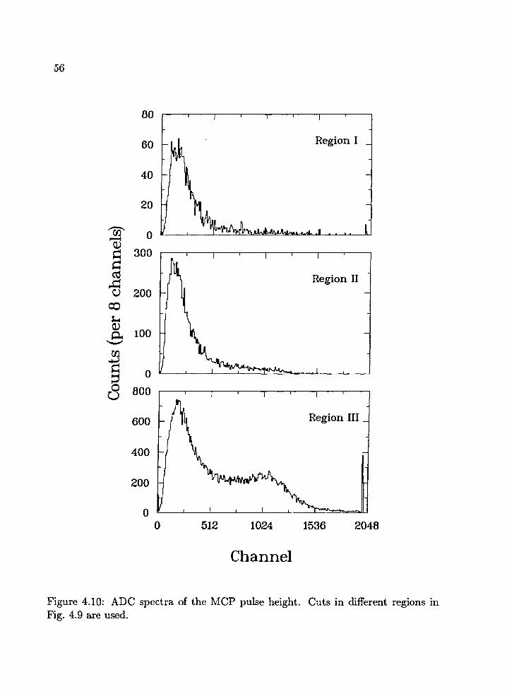
4.10 ADC spectra of the MCP pulse height. Cuts in different regions in
Fig. 4.9 are used 56
viii
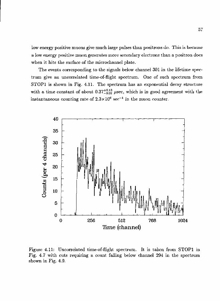
4.11 Uncorrelated time-of-flight spectrum. It is taken from STOP1 in
Fig. 4.7 with cuts requiring a count falling below channel 294 in the
spectrum shown in Fig. 4.9 57
4.12 Time-of-flight spectra of negative muonium ions taken with Al foil.
The momentum of the incident positive muon beam was 9.75 MeV/c.
The timing is reversed 59
4.13 TDC spectrum for the lifetime measurements of negative muonium
ions with Al foil 61
4.14 Michel spectrum of decay positrons from negative muonium ions. . . 62
5.1 Nal spectrum taken with positive muons at the end of the straight
channel for the energy calibration of the detector 66
5.2 Nal spectrum taken with positive muons at the end of the 60°-channel
for the energy calibration of the detector 68
5.3 Nal spectrum taken with negative muonium ions at the end of the
60°-channel 68
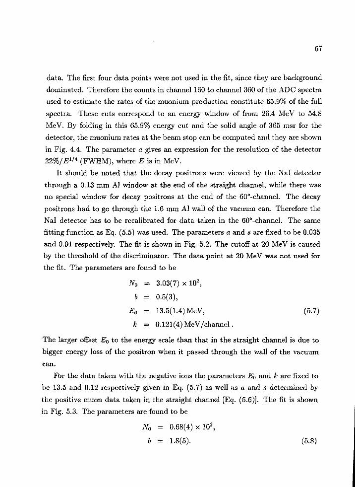
5.4 Time spectrum of the decay positrons from positive muons at the
end of the 60°-channel 70
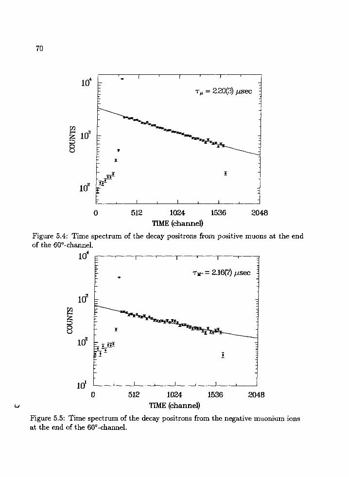
5.5 Time spectrum of the decay positrons from the negative muonium
ions at the end of the 60°-channel 70
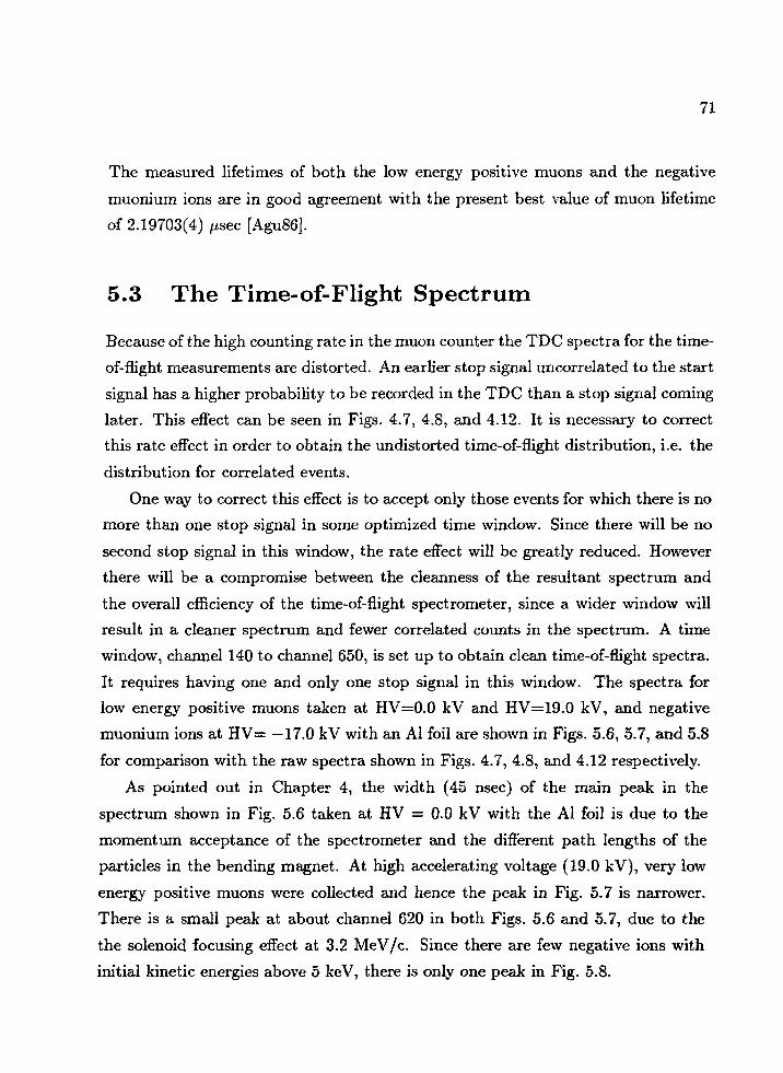
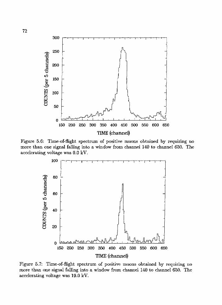
5.6 Time-of-flight spectrum of positive muons obtained by requiring no
more than one signal falling into a window from channel 140 to chan-
nel 650. The accelerating voltage was 0.0 kV 72
5.7 Time-of-flight spectrum of positive muons obtained by requiring no
more than one signal falling into a window from channel 140 to chan-
nel 650. The accelerating voltage was 19.0 kV. 72
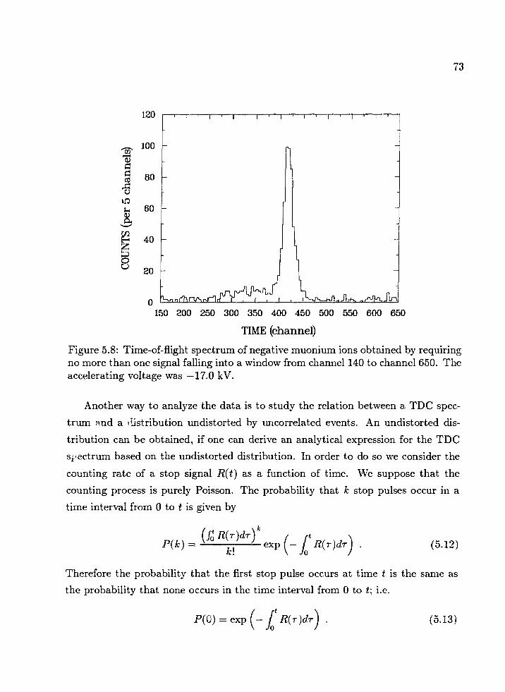
5.8 Time-of-flight spectrum of negative muonium ions obtained by re-
quiring no more than one signal falling into a window from channel
140 to channel 650. The accelerating voltage was —17.0 kV 73
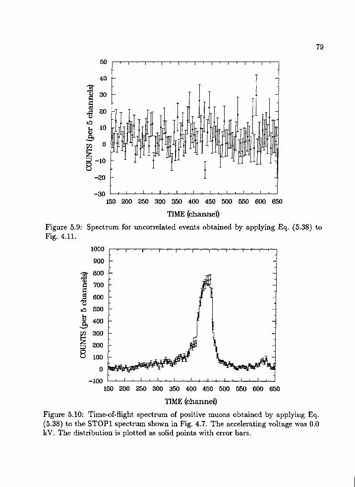
5.9 Spectrum for uncorrelated events obtained by applying Eq. (5.3S) to
Fig. 4.11 79
ix
5.10 Time-of-flight spectrum of positive muons obtained by applying Eq.
(5.38) to the STOPl spectrum shown in Fig. 4.7. The accelerating
voltage was 0.0 kV. The distribution is plotted as solid points with
error bars 79
5.11 Time-of-flight spectrum of positive muons obtained by applying Eq.
(5.38) to the STOPl spectrum shown in Fig. 4.8. The accelerating
voltage was 19.0 kV. The distribution is plotted as solid points with
error bars SO
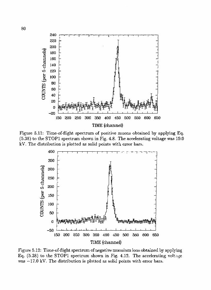
5.12 Time-of-flight spectrum of negative muonium ions obtained by ap-
plying Eq. (5.38) to the STOPl spectrum shown in Fig. 4.12. The
accelerating voltage was —17.0 kV. The distribution is plotted as
solid points with error bars 80
5.13 Time-of-flight spectrum of positive muons decelerated by —24.2 kV.
The smooth curve is a fit to the data using function (5.39) 81
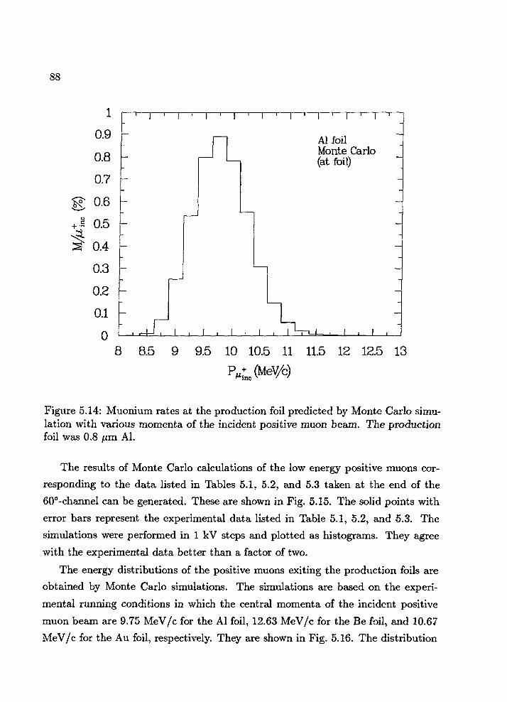
5.14 Muonium rates at the production foil predicted by Monte Carlo sim-
ulation with various momenta of the incident positive muon beam.
The production foil was 0.8 jum Al 88
5.15 Low energy positive muon rates at the MCP detector with various
accelerating voltages 89
5.16 Energy distributions of outgoing positive muons from (a) Al foil, (b)
Be foil, and (c) Au foil calculated with the Monte Carlo code 90
5.17 Rates of negative muonium ions at focal plane with Al foil. The
histogram represents the Monte Carlo simulation 91
5.18 Rate of negative muonium ions at focal plane with Be foil. The
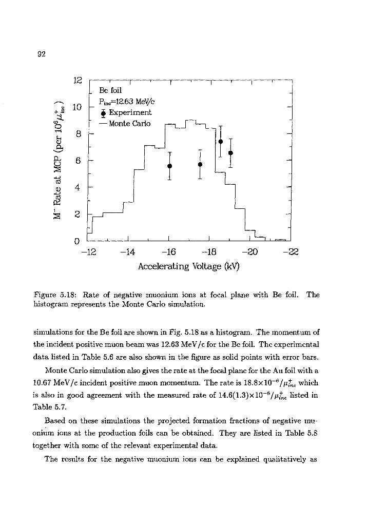
histogram represents the Monte Carlo simulation 92
5.19 Angular distributions of (a) fi+, (b) M, and (c) M~ coming out of
Al foil. The momentum of the incident positive muon beam was
centered at 9.75 MeV/c 94
5.20 Angular distributions of (a) /x+, (b) M, and (c) M~ coming out of
Be foil. The momentum of the incident positive muon beam was
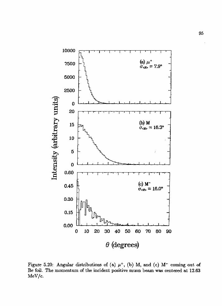
centered at 12.63 MeV/c 95
x
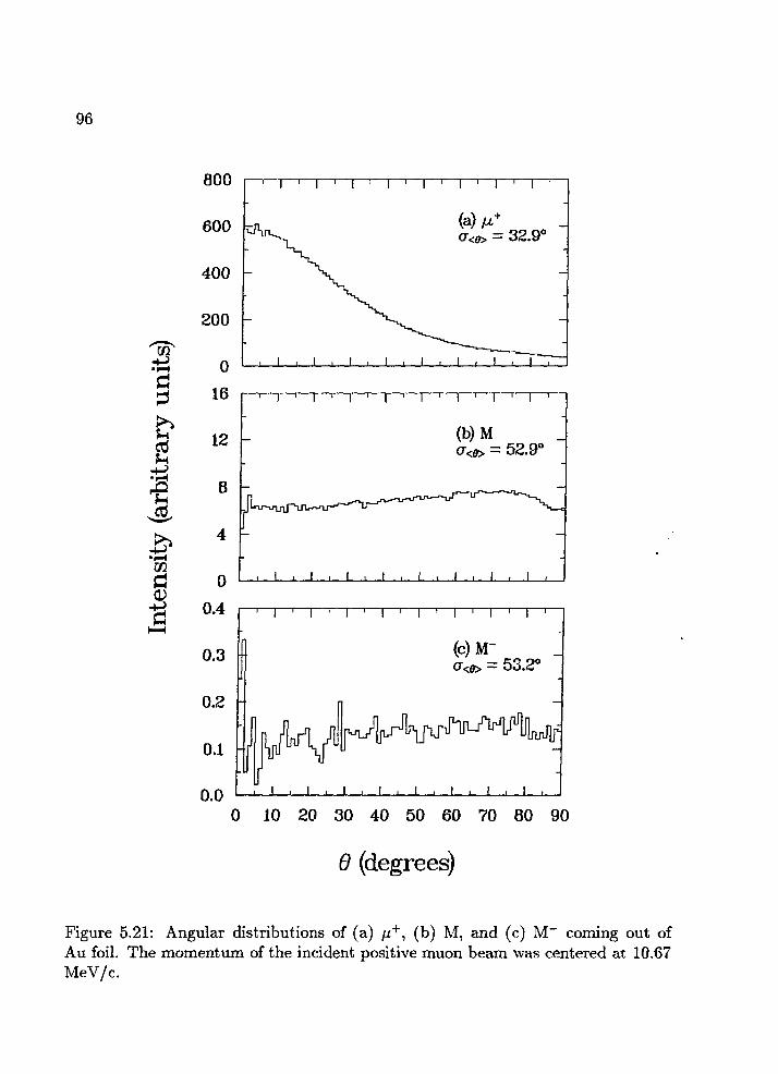
5.21 Angular distributions of (a) /x+, (b) M, and (c) M coming out of
Au foil. The momentum of the incident positive muon beam was
centered at 10.67 MeV/c 96
5.22 Time-of-flight spectra of positive muons, (a) Monte Carlo, (b) mea-
surement 97
A.I Muonium rates at beam stop for different momenta of incident beam. 108
A.2 Muonium rates at production foil for different momenta of incident
beam 109
A.3 Positive muon rates at the MCP beam stop for different accelerating
high voltages with (a) Al, (b) Be, and (c) Au foils. The solid points
with error bars are the experimental data from Ref. [Kua87] I l l
A.4 Energy distribution of positive muons from Al foil. The momentum
of the incident positive muon beam was 9.75 MeV/c 112
A.5 Energy distributions of positive muons, muonium atoms, and nega-
tive muonium ions below 40 keV from Al foil 112
A.6 Angular distributions of positive muons (a), muonium atoms (b), and
negative muonium ions (c) 114
x i
List of Tables
2.1 Binding energies of H , M , and Ps , and their electron affinities
calculated based on [Pet87j. The reduced masses are also listed. . . 6
3.1 Properties and thicknesses of foils used as charge capture media in
the experiment 21
4.1 Average rates of fj,fnc, rates in Nal and projected rates of muonium
atoms at the beam stop 48
4.2 Average rates of fifnc, interrupt rates and raw rates of positive muons
taken with Al foil at various accelerating voltages. The momentum
of the incident positive muon beam was 9.75 MeV/c 53
4.3 Average rates of (j,fnc, interrupt and raw rates of positive muons taken
with Be foil at various accelerating voltages. The momentum of the
incident positive muon beam was 12.63 MeV/c 54
4.4 Average rates of fj,fnc, interrupt and raw rates of positive muons taken
with Au foil at various accelerating voltages. The momentum of the
incident positive muon beam was 10.67 MeV/c 54
4.5 Average rates of fifnc, interrupt rates, and raw rates of negative mu-
onium ions taken with Al foil at various accelerating voltages. The
momentum of the incident positive muon beam was 9.75 MeV/c. . . 58
4.6 Average rates of /U2+c, interrupt rates, and raw rates of negative mu-
onium ions taken with Al foil at various accelerating voltages. The
momentum of the incident positive muon beam was 9.75 MeV/c. The
spectrometer settings were scaled down by a factor (1.415) 60
xii
4.7 Average rates of /i£ic, interrupt rates, and raw rates of negative mu-
onium ions taken with Be foil at various accelerating voltages. The
momentum of the incident positive mucn beam was 12.63 MeV/c. . 63
4.8 Average rate of fifnc, interrupt rate, and raw rate of negative muon-
ium ions taken with Au foil. The momentum of the incident positive
muon beam was 10.67 MeV/c 63
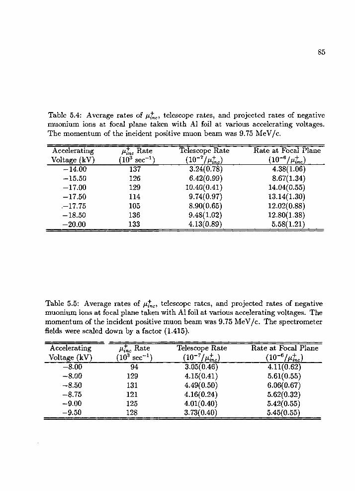
5.1 Average rates of fj,fnc, telescope rates, and projected rates of low
energy positive muons at focal plane taken with Al foil at various
accelerating voltages. The momentum of the incident positive muon
beam was 9.75 MeV/c 83
5.2 Average rates of fj.fnc, telescope rates, and projected rates of low
energy positive muons at focal plane taken with Be foil at various
accelerating voltages. The momentum of the incident positive muon
beam was 12.63 MeV/c 84
5.3 Average rates of /u^c, telescope rates, and projected rates of low
energy positive muons at focal plane taken with Au foil at various
accelerating voltages. The momentum of the incident positive muon
beam was 10.67 MeV/c 84
5.4 Average rates of fifnc, telescope rates, and projected rates of negative
muonium ions at focal plane taken with Al foil at various accelerating
voltages. The momentum of the incident positive muon beam was
9.75MeV/c 85
5.5 Average rates of nfnc, telescope rates, and projected rates of negative
muonium ions at focal plane taken with Al foil at various accelerating
voltages. The momentum of the incident positive muon beam was
9.75 MeV/c. The spectrometer fields were scaled down by a factor
(1.415) 85
xiii
5.6 Average rates of fj,fnc, telescope rates, and projected rates of negative
muonium ions at focal plane taken with Be foil at various accelerating
voltages. The momentum of the incident positive muon beam was
12.63 MeV/c 86
5.7 Average rate of nfnc, telescope rate, and projected rate of negative
muonium ions at focal plane taken with Au foil. The accelerating
voltage on the accelerator was —17.5 kV. The momentum of the
incident positive muon beam was 10.67 MeV/c 86
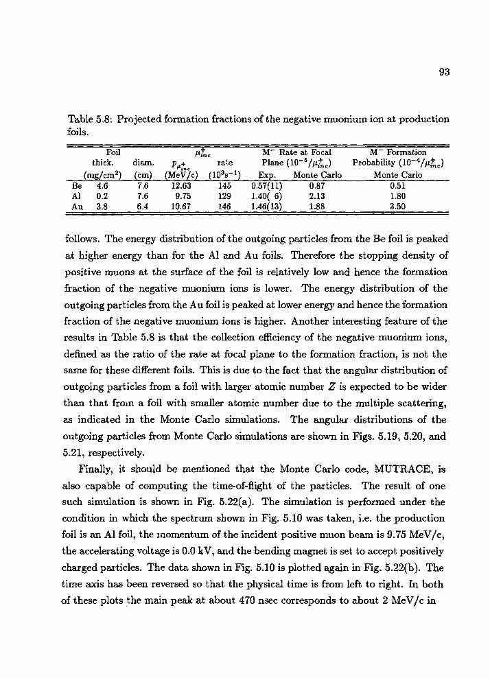
5.8 Projected .formation fractions of the negative muonium ion at pro-
duction foils 93
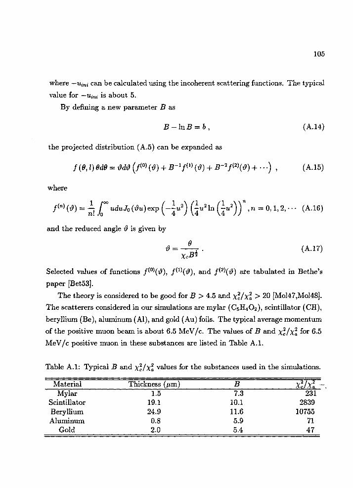
A.I Typical B and Xc/Xo vahies for the substances used in the simulations. 105
A.2 Rates of negative muonium ions at MCP with different production
foils. The experimental data are taken from [Kua87] 110
xiv
Acknowledgement s
I am greatly indebted to my thesis advisor, Professor Vernon W. Hughes, for his
guidance and support throughout the last four years. I thank Dr. Herbert Orth
for his invaluable advice and encouragement during the design and execution of the
experiment. My thanks go to my other coworkers, including Klaus-Peter Arnold,
Frank Chmely, Morton Eckhause, John Kane, Steve Kettell, Krishna Kumar, Daniel
Lu, Bjorn Matthias, Benwen Ni, Reiner Schaefer, Paul Souder, and Kim Woodle
for their patience and contributions to my education.
I also thank Joe Ivie, Seth Rislove, Richard Werbeck, and the LAMPF staff
without whose help the experiment would never have been possible.
I would like to express my gratitude to Dr. T. D. Lee and the CUSPEA commit-
tee for providing me with the opportunity to study at Yale University. I thank the
Yale University Graduate School for the Yale Scholarships and Fellowships which I
received during the first two years of my graduate studies.
Finally, I would like to thank Sara Batter, Gina Canali, Pat Fleming, Debbie
McGraw, Leonard Roote, Wilma Thiel, and Barbara Voiges for everything.
xv
Abstract
The negative muonium ion (M ), which is the bound system of a positive muon
and two electrons, has been produced and observed for the first time [Arn86,Har86,
Kua87]. Its counterpart H~ is well known, and spectroscopy and collision studies
with H~ Lave yielded many fruitful results. Noteworthy are recent) investigations
of the photoionization of a relativistic H~ beam [Bry81]. The negative positronium
ion has also been formed and observed [Mil81b]. The discovery of M~ provides us
with a new leptonic system for spectroscopy and collision studies?, which may reveal
interesting physics associated with mass effects. Since M~ is a charged particle, it
can also be used to produce a beam of exotic atoms with a small phase space. This
dissertation is a detailed account of the observation of M~.
The experiment was conducted at LAMPF, utilizing a subsurface fi+ beam
[Bad85] and the beam-foil technique. When a fi+ beam of about 10 MeV/c mo-
mentum passes through a thin foil, the outgoing species are //+, M, and M~ due to
charge exchange of fi+ with the foil material. In the experiment, the M~ ions were
accelerated electrostatically to about 20 keV. A magnetic spectrometer selected the
negatively charged particles and bent the ion beam by 60° relative to the direction of
the incoming beam. The ions were then focused by a solenoid onto a microchannel
plate detector (MCP). Two pairs of scintillators were mounted around the MCP to
detect the decay positrons for the measurement of the muon lifetime. The incident
fi* beam was monitored by a thin plastic scintillation counter. The time-of-flight of
the particles from the muon counter to the MCP detector was measured. The M~
was identified in the experiment as a particle of unit negative charge with a mass of
about 107 MeV/c2 and the lifetime of the muon. The fact that the system contains
xv i
a muon was further confirmed by the characteristic Michel energy spectrum of the
positrons from muon decay measured with a Nal(Tl) detector. Three foil materials
(Al, Au, Be) were used in the experiment. The M~ yield at the focal plane was
about 1.4 x 10~5/fifnc.
In addition, the low energy positive muons of up to 20 keV kinetic energies
coming out of the foils were investigated. The results provide information on the
energy distribution and the angular distribution of the emerging fi+ beam.
A Monte Carlo scheme of simulating the energy loss, the multiple scattering,
and the charge equilibrium states and of computing the time-of-flight has been
developed. The results are compared with experimental data and good agreements
are found. The Monte Carlo code can thus be used to predict results of future
beam-foil experiments.
xvii
Chapter 1
Introduction
The negative hydrogen ion H has been known since the development of quan-
tum mechanics [Bet29,Bet33] and over the decades many spectroscopy and collision
studies of H~ have been made [Mas69,Bet77]. Recently, photoionization of rela-
tivistic H~ beams has been investigated [Bry81]. Moreover, E~ beams are playing
ari important role in several major accelerator laboratories.
H~ can be produced by the beam-foil method [Phi55]. When a proton beam
passes through a thin foil, the protons undergo charge capture and loss processes.
A fraction of the piotons will capture one electron to form hydrogen atoms, a
small fraction can capture two electrons to form H~. For many reasons the charge
changing processes have drawn great attention [All58,Taw73].
The leptonic atoms, positronium, Ps (e+e~), and muonium, M (/i+e~), are im-
portant simple systems for the study of fundamental interactions and atomic struc-
ture. Leptons are believed to be structureless particles. Because of the absence
of the size effect of the nucleus, the structure of leptonic atoms can, in principle,
be computed very precisely by Quantum Electrodynamics (QED). Experimental
measurements of their structure, therefore, provide rigorous tests of the theory.
Muonium was first produced in vacuum by the beam-foil method [BolSl]. Since
then, great effort has been devoted to measure the Lamb shift of the muonium
atom in the n = 2 state [Ora84,Bad84], although improvement on the experimental
precision is necessary in order to compete with the precision of theoretical compu-
tations [Owe73]. Recently, the M system has also been used in order to probe the
lepton number conservation law adopted by the standard model of the electroweak
interaction [Gla61,Sal68,Wei67]. A search for spontaneous conversion of muonium
to antimuonium was conducted, leading to an upper limit on the coupling constant
of G M M < 7.5GF (at 90% confidence level) [Ni87].
On the other hand, Ps was also found by the beam-foil method [Can74,Mil85]. A
measurement of the decay rate of orthopositronium ( 1 3 SI ) has shown a discrepancy
with theory [Gid78,Wes87]. The present theoretical calculation of the decay rate has
been carried out to 0(a2ln(a~1)). Higher order corrections are therefore needed.
The positronium negative ion, Ps~ (e+e~e~), was also observed [Mil81b], which led
to measurements of its annihilation lifetime [Mil83].
The negative muonium ion, M~ (/x+e~e~), can be produced in a similar fashion
by the beam-foil method. Since a positive muon beam is easily obtainable in many
laboratories, the charge capture process to form the negative muonium ion can be
studied in great detail. Comparisons between the three different negative ions H~,
M~, and Ps~ in spectroscopy and collision studies may reveal interesting physics
associated with mass effects and lead to a better understanding of these three-body
systems.
Recently, the thermal muonium atom has been produced with greater efficiency
[Mil86,Bee86]. However, muonium atoms in the n — 2 metastable state are not
expected to be formed with comparable efficiency in the thermal energy regime.
Formation of muonium in the 2S state is essential for the Lamb shift measurement.
Since M~ is charged, it is possible to form a beam of exotic atoms with a very small
phase space by accelerating the ions to higher energy. This beam may be useful for
further measurements of the muonium n = 2 Lamb shift.
The production and observation of the negative muonium ion in a beam-foil
experiment is the main subject of this dissertation. The results of the studies on low
energy /j,+ will also be given. They will be compared with Monte Carlo simulations.
The principles and theories will be discussed in Chapter 2. In Chapter 3, the
experimental techniques and the apparatus will be described. The observations and
data analysis will form the contents of Chapter 4 and 5. Discussion of the results
will be given in Chapter 6. The Monte Carlo code, MUTRACE, is described in
Appendix A.
Chapter 2
Physical Principles
The experiment utilized a fi+ beam originating from positive pions stopped some
distance from the surface inside the target for the primary proton beam. This fi+
beam is called a "subsurface" /z+ beam. When a fx+ beam passes through a thin
foil, some fraction of the /J.+ will capture one electron to form muonium atoms, and
a smaller fraction should capture two electrons to form negative muonium ions. The
physical principles underlying the production and the observation of the negative
muonium ion will be presented in this chapter. Some properties of the ion will also
be discussed.
2.1 Properties of the Negative Muonium Ion and
Muon Decay
The negative muonium ion (M~) is a bound system of a positive muon (/x+) and two
electrons (e~). It is a light isotope of H", the negative hydrogen ion. Since the muon
mass is about one ninth that of the proton and about 207 times that of the electron,
M~ is expected to have similar properties to H~. Because of the importance of H~
to astrophysics and atomic collisions and its simplicity as a negative ion, it has
drawn attention of both theorists and experimentalists. An energy level diagram
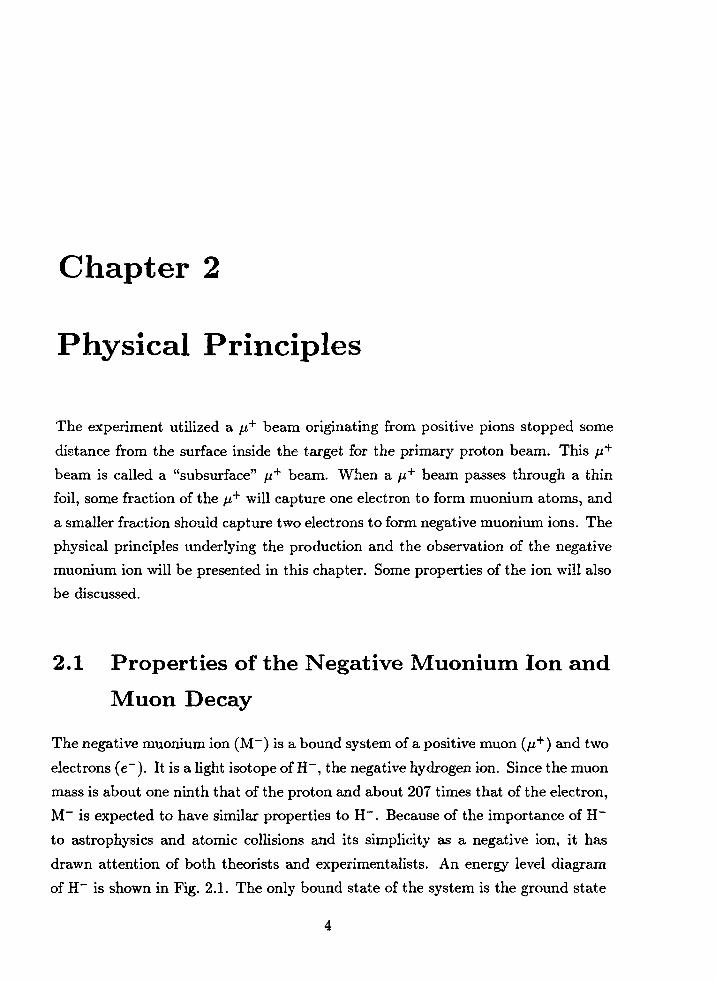
of H~ is shown in Fig. 2.1. The only bound state of the system is the ground state
1So. All other states are autoionizing states except a metastable 2p2 3P e state, as
yet unobserved, 0.0095 eV below the energy level of a n = 2 hydrogen atom and a
free electron [Dra70].
14
13
12
11
I 1 0a
IoX
>
9
8
7
6
5
4
w 3
2
1
0
-1
— H(n=2)+e"
H(n=l)+e" -
lg 3g 3p Ij)
Figure 2.1: Lowest energy levels of H based on [Bur68].
The ground state of M" has a binding energy of 0.525 a.u. (14.287 eV) based
on theoretical calculations [Pet87]. The electron affinity, which is the binding
energy against breaking up into a muonium atom and a free electron, is there-
fore about 0.0275 a.u. (0.747 eV). The binding energies of H", M~, and Ps~
are listed in Table 2.1 for comparison. The values of the fundamental constants,
Table 2.1: Binding energies of H~, M~, and Ps~, and their electron affinities calcu-lated based on [Pet87]. The reduced masses are also listed.
Ion Binding Energy Electron Affinity Reduced Mass(eV) (eV) (in electron mass units)
me = 0.51099906(15) MeV/c2, mM = 105.658389(34) MeV/c2, mv = 938.27231(28)
MeV/c2, and R^ = 13.6056981(40) eV, are taken from [Cob36]. One can see that
the binding energies are approximately proportional to the reduced masses. How-
ever, these are three-body systems, so that mass-polarization and other effects will
certainly have influence on the energy levels. One of the interesting consequences is
that the energy levels of the 2p2 3P e states of H" and M~ are below n = 2 threshold,
while that of the 2p2 3Pe state of Ps~ is not [Mil81a,Bha83].
The photodetachment cross section of M~ has been computed recently. The
maximum is on the order of 10~17 cm2 [Bha87]
Since M~ contains a /i+, it will be advantageous to detect the /i+ when confirming
the observation of the ion. The positive muon decays via
V+ -+ e+ueV, (2.1)
with a lifetime of 2.19703(4) fisec [Agu86]. It is a three-body decay. Thus, the
decay positron has a continuous energy spectrum, the so-called Michel spectrum
[Mic50,Com83]. Let us define the following parameters
W = (m2 + m
x = EJW, (2.2)
xQ = me/W,
where Ee is the energy of the decay positron, m^ the muon mass, and me the
electron or positron mass. The differential decay probability for a positron with
energy between x and x + dx, emitted at an angle between 0 and 6 -f- d8 with
respect to the muon spin direction is given by
dxd(cos9) ~
+ Jx2 - xl{2x - 1 - —io)cos0} , (2.3)
where GF = 1.16637(2) X 10~5GeV~2 is the Fermi coupling constant in units where
h = c = 1. The radiative corrections are not included in the expression. Both the
muon lifetime and the Michel spectrum can be measured in the experiment.
2.2 Charge Capture Processes
It has long been recognized that charge transfer processes play an important role
in atomic collisions and have been studied by many experimentalists and theorists
[A1158,Taw73]. A great deal of work has been done on hydrogen passing through
gaseous targets. For a proton in gas the processes can be described as follows. A
particle experiences electron capture and loss processes during its traveling through
the gas. After it travels a certain distance, equilibrium is reached. For a three-
component system, such as H", H°, and H+ , there are six charge-changing processes.
The corresponding cross sections are a+0, 0"+-, cr0-, 0o+, °"-o, and <?-+. They
represent single and double electron capture by H+, single electron capture and loss
by H°, and single and double electron loss by H~, respectively. The equilibrium
condition for the charge states can be written as
(<7+o -f 0-+_)ra+ — ao+no — cr-+n- = 0 ,
cr+on+ — (<ro+ + crO-)no + <7-o«- = 0 , (2.4)
ra+ + «o + " - = n ,
where n+ , no, and n_ are the numbers of H~, H°, and H+, respectively. The fractions
of the charge states are therefore
* — !?£ _ + ^H—^-O + cr+o<7-+77- iJ
d> - n ~ - ao-a+- + <7Q+cr+- + cr+ocro-*~ ~ n " D '
where
o_cr+_ + cr0+cr+_ + CT+O<TO_ . (2-8)
The electron capture processes by a proton in solids is much more complicated.
The three charge states for hydrogen ions from solids were first intensively studied
by Phillips [Phi55]. The experiment was repeated later with a deuterium beam
[Ber72]. The general observations of the charge capture processes are that the
fraction of a charge state is 1) strongly dependent on the velocity of the projectile,
2) weakly dependent on the target material, and 3) independent of the mass of
the projectile. Therefore, a velocity scaling rule can be applied, i.e., the charge
fraction for a positive muon is the same as that for a proton at the same velocity.
This scaling rule was verified down to 4 keV/amu in both transmission experiments
[Phi55,Ber72] and backscattering experiments [Bha80,Eck76] in which the charge
fractions of reflected particles were measured.
Based on the proton data [Phi55], the fractions of the charge states for muonium
ions emerging from a solid foil can be plotted as a function of the energy as shown in
Fig. 2.2. Most of the neutral muonium atoms have less than 20 keV kinetic energy,
while the fraction of the negative muonium ions only becomes significant for kinetic
energies below 5 keV. The integrated rate of production of the negative muonium
ions is about two orders of magnitude lower than that of the neutral muonium
atoms.
It appears that the conventional description of the charge state equilibrium of
particles at higher velocities (> Z2^3VQ, where vo is the Bohr velocity of 2.2 x 10⁸
cm/sec.) in gases can be adapted to solids. At these velocities, the capture and
loss processes are due to the interaction with the inner shells of the target atoms.
A particle experiences electron capture and loss processes as it travels through the
solid, and the equilibrium of the charge states is obtained after some collisions.
100
80
g, 60
40
I0
0 205 10 15KE (keV)
Figure 2.2: Charge fractions of emerging muonium ions.
The charge-state fractions can then be obtained using cross sections computed for
gaseous targets. This picture has been successfully used to describe the neutral
fraction emerging from solid carbon with incident protons [Cro77]. Since the fraction
of the negative ions is very small at these velocities, a two-component system,
i.e. positive and neutral states, is assumed.
However, the concept of capture and loss inside a solid may be meaningless for
velocities below the Fermi velocity of the electrons in the solid. (A typical metal
Fermi velocity is about the same as the Bohr velocity i>0.) In this case, because of the
collective screening by the target electrons in a solid or collision broadening of the
bound states, there is no bound state in the solid [Bra75b]. Therefore, the surface
effects become important. At the surface, processes such as Auger-neutralization,
resonance-neutralization, and resonance-ionization can take place [Hag54]. The
recombination process [Kit76] can also occur. However, due to the complexity of
10
the processes, there is no single theory which can explain all experimental data.
At low velocities (< v0) formation of the negative ions becomes significant. The
fraction of the negative ions increases monotonically with decreasing energy down
to 4 keV/amu [Phi55,Ber72]. In fact, it was found that the fractions of H° and H~
depend exponentially on energy in the region from 30 to 340 keV [Ros86]
* = ex?(-(E + E0)/E1) , (2.9)
where E is the kinetic energy of the ions, Eo and Ei are the fitting parameters.
For H~, EQ is about 136 keV and Ei is about 35.4 keV. The processes were also
studied in a backscattering experiment for energies below 4 keV/amu [Ver80]. As
the energy decreases, $_ reaches a maximum at about 3 keV/amu [VerSO] for most
metallic surfaces. A strong correlation between the work function of the target
material and the formation fraction of the negative ions was observed [Yu78]. As
the work function decreases, the maximum of the charge fraction moves towards
lower energy and the amplitude of the maximum increases.
The theories for the formation of the negative ions at a surface are developed
for alkali covered surfaces. The general description is that an H+ is first neutralized
near the surface, then captures another electron at some distance from the surface.
It may then lose an electron by resonance-neutralization [His79]. The production
of the negative ion can be written as a product of the formation probability and
the survival probability. Assuming these are adiabatic processes, that is the atom
moves slowly with velocity v± normal to the surface, the formation probability can
be qualitatively written as
l-exp(-a/ t7j . ) (2.10)
and the survival probability is
exp(-0/vx) , (2.11)
where a and /? are constants, independent of the exit angle of the ion. Therefore,
the fraction of the negative ions is
$_ ~(l~exp(-a/t?x))exp(-/3/wj.) . (2.12)
11
Comparison between this model and the experimental data shows that Eq. (2.12)
gives a reasonable trend for alkali metal surfaces such as Cs. However it can not be
applied directly to other metal surfaces. In fact an angular dependence of a and /?
has been found [Ver80]. At present, there is no reliable theory for the formation of
negative ions in beam-foil experiments.
2.3 Subsurface Positive Muon Beam
To achieve a high formation fraction of negative muonium ions, one has to obtain
large number of low energy (v < v0) positive muons at the exit surface of the foil
target. Therefore, a positive muon beam of high stopping density is required- The
positive muon beam can be produced via the reactions
p + N —»• 7r+ + fragments
where p is a proton and N is a target nucleus. The TT+ production is achieved by
bombarding a carbon target with a proton beam of energy above the threshold T4,
which is given by (see for example [Bet55])
m 2m
Tt ~ 2m* + — 2 - ~ 290 MeV , (2.13)2m
where mv = 139.57 MeV/c2 is the pion mass and mjy — 940 MeV/c2 is the nucleon
mass. The y,+ originating from 7r+-decay can then be collected. An effective way
of producing a high stopping density /x+ beam was developed by Pifer, Bowen, and
Kendall [Pif76] in which /z+ from n+-decay at rest are directly collected off the
primary beam target surface. The /i+ from ?r+ decay (r = 26.03 nsec.) at rest has
an isotropic angular distribution. Its energy and momentum are
E * " = 109.78 MeV, (2.14)
2
Pti = m * m " = 29.79 MeV/c , (2.15)2m
12
where m^ = 105.66 MeV/c2 and the neutrino mass is assumed to be zero. Because
of nonconservation of parity in the weak interaction the neutrino is assumed to have
always left handed helicity. The /x+ from 7r+-decay are therefore fully polarized with
negative helicity in order to conserve momentum and spin.
The range of the /x+ in this momentum region is approximately given by [Tro66]
R = kpa (2.16)
as a function of momentum p, where k is a constant that depends on material and
a ~ 3.5. The range spread is therefore given by
AR = aRAp/p . (2.17)
Taking into account a range straggling of 10% of the range [Ste60], the total range
spread can be written as
AR = kpa^/(0.iy + (aAp/p)2 . (2.18)
In order to obtain a high formation fraction of M and M~, a high stopping
density fx+ beam is desirable. As one can see, a low-momentum fx+ beam should be
used. The (i+ beam utilized in this experiment had a momentum between 8 MeV/c
and 14 MeV/c. It was obtained by collecting //+ originating from positive pions
stopped some distance inside the surface of the primary proton target. This beam
is referred to as a subsurface fi+ beam [Bad85].
Chapter 3
Experimental Technique and
Apparatus
The experiment employed a beam-foil method and utilized a subsurface beam of pos-
itive muons. The stopped muon channel (SMC) at the Los Alamos Meson Physics
Facility (LAMPF) was tuned to a low-momentum subsurface fi+ beam [Bad85], such
that the peak of the stopping profile was centered near the downstream surface of
the production foil. The positron contamination of the //+ beam was greatly re-
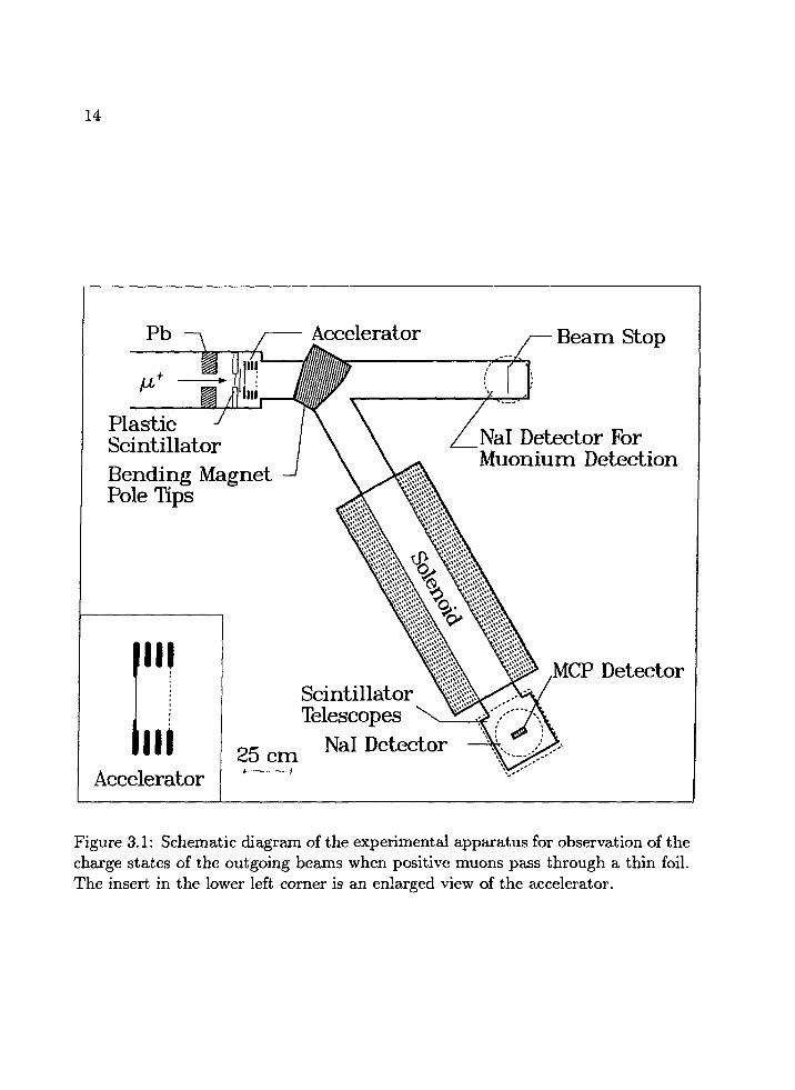
duced by using a Wien filter. The experimental apparatus is shown in Fig. 3.1. The
purified positive muon beam had a momentum p^ of about 10 MeV/c and Ap^/p^
of 10% (FWHM). The average intensity was 140xl03 sec"1 through a 7-cm thick-
lead collimator with a 6% duty cycle. The beam passed through a thin 2 mg/cm2
scintillator which served both as a degrader and as a muon counter, and a 0.2
mg/cm2 aluminum protection foil which prevented sparking at high voltage. The
production foil was mounted on the high-voltage end of an electrostatic accelerator
column capable of operation up to ±25 kV, while a highly transparent copper mesh
held at ground potential maintained a uniform accelerating field. Three different
foils were used as charge exchange media. The particles were selected for charge
state and momentum by a wedge-shaped 60° bending magnet with double-focusing
properties symmetric about the central trajectory of the particles. A solenoid of 130
cm length and 712.5 G central field transported the ions away from the direct beam
13
14
Accelerator
PlasticScintillatorBending MagnetPole Tips
Beam Stop
Nal Detector ForMuonium Detection
25 cm
ScintillatorTelescopes
Nal Detector
W ,MCP Detector
Figure 3.1: Schematic diagram of the experimental apparatus for observation of thecharge states of the outgoing beams when positive muons pass through a thin foil.The insert in the lower left corner is an enlarged view of the accelerator.
15
into a low background region. As a result of its fringe field, this solenoid focused the
beam onto a microchannel plate (MCP) detector. The decay positrons from positive
muons were observed in either of two pairs of scintillator telescopes installed above
and below the MCP (Fig. 3.2). The characteristic Michel energy spectrum of the
Solenoid
Horizontal V
C2c
lew
MCP
Nal
^> Scintillators
Vacuum/Chamber
^> Scintillators
Figure 3.2: The horizontal view of the detector arrangement at the end of the 60°channel.
decay positrons was taken with a Nal(Tl) detector. Neutral muonium atoms were
stopped directly downstream in the straight channel on a Teflon plate subtending a
solid angle of about 8 msr at the production foil. Decay positrons from this beam
stop were also observed with another Nal(Tl) detector. Time-of-flight spectra were
16
taken between the muon counter (plastic scintillator), microchannel plate, and scin-
tillator telescopes. The data were read into a PDP-11/34 computer via a CAMAC
interface. The technical details will be described in the following sections of this
chapter.
3.1 Separated Subsurface Beam of Positive Muons
The linear accelerator at LAMPF provided an 800 MeV proton beam with an aver-
age current of 635 /iA and a duty cycle of 6.0% [LAM80]. The proton beam had a
microstructure of nanosecond-wide bursts separated by 5 nsec and a macrostructure
consisting of 500-^sec bursts at a rate of 120 sec""1. The proton beam went through
the A-2 production target which was nominally carbon, producing pions in the tar-
get region. The subsurface positive muon beam, originating from positive pions
stopped in the A-2 production target, was transported through the stopped muon
channel (SMC) [Tho79]. Figure 3.3 shows the layout of the channel, which consists
of 21 quadrupole magnets and 4 bending dipole magnets. The overall length of the
channel is about 30 m. The channel was originally designed for a muon beam from
pions decaying in flight as well as for a pion beam. It can be viewed as having three
separate sections: (1) a pion collection and analyzing portion, (2) a 7r-decay and
muon collection portion, and (3) a pion rejection and muon momentum analysis
portion. However, it was used to transport a subsurface positive muon beam of 8
MeV/c to 14 MeV/c momentum in this experiment by simply tuning the channel
to low momentum. The typical phase space of the subsurface /x+ beam in the west
cave (CAVE A) is [Bad85]
ax • ax< — 95 cm • mrad ,
oy • <Tyi = 46 cm • mrad , (3.1)
^ = ±5%.P
The channel was extended with six quadrupole magnets and a Wien filter,
(E x B) separator, to reduce e+ contamination in the [i+ beam. The extension
is shown in Fig. 3.4. The quadrupole magnets were arranged to be FDDFFD in the
Figure 3.3: Layout of the stopped muon channel (SMC). The present experimentwas carried out in the west cave (CAVE A).
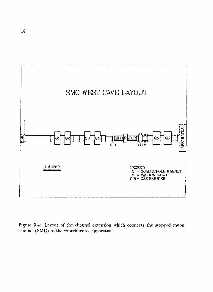
18
SMC WEST CAVE LAYOUT
Ql Q2 Q3
G.B.
Q5 Q6
1 METER LEGENDQ = QUADRUPOLE MAGNETV = VACUUM VALVE
G.B.= GAS BARRIER
Figure 3.4: Layout of the channel extension which connects the stopped muonchannel (SMC) to the experimental apparatus.
19
horizontal plane, where F and D stand for focusing and defocusing, respectively. It
was attached directly to the valve SV-A of the SMC. The separator has two" high
voltage plates of 100 cm long and 15 cm wide, and the gap between the plates is
10 cm. The effective length of the magnetic field region is 38 cm. The magnetic
field was set at 300.55 G. The corresponding electric field for transmitting parti-
cles with velocity f3c is given approximately by E (kV/cm) = 112/3B (kG). In the
experiment, the electric field was tuned to maximize the positive muon rate. The
optimum was found at 2.95 kV/cm for 9.75 MeV/c positive muons. A Monie Carlo
calculation of the transmission efficiency was performed using the computer code
MUTRACE, which is described in Appendix A. The transmission efficiency was
found to be 74% for 9.75 MeV/c positive muons, while the transmission efficiency
for positrons at 9.75 MeV/c was less than 0.01% . The e+ contamination was re-
duced to e+//u+ < 4. Most of the positrons which went through the channel were
from positive muons decaying in flight. The e+ contamination is higher than that
reported before [Bad85] due to the unequal lengths of E and B field regions in the
separator which prevented us from increasing the fields.
Radioactive gas in the channel was another major source of background [Bad85]
Because of the high temperature of the A-2 production target (400 K at an average
proton current of 650 fiA), the gaseous, radioactive spallation products with a mean
lifetime of the order of 1 sec diffuse out of the target before they decay. It is
necessary to reduce the radioactive gas in our experimental apparatus, since the
thin scintillation counter and the microchannel plate detector are very sensitive to
them. The main components of the radioactive gas are 6He (ti/2 = 0.S07 sec.) and12N (<i/2 = 0.011 sec). A gas barrier of 1.5 fan mylar was inserted in the beam
line between the separator and the downstream apparatus. The purpose of the gas
barrier was the following. It left the vacuum upstream at about 5 x 10~3 Torr, thus
retarding the diffusion of the radioactive gas such that most of it decayed before
reaching the gas barrier. The downstream vacuum was about 3 x 10~6 Torr. The
1.5 jum gas barrier itself can effectively prevent nitrogen from diffusing through.
The positive muon rate was monitored by a thin plastic scintillator. The beam
spot size at the scintillator was about 5 cm (FWHM), as was calculated using the
20
computer code TRANSPORT [Bro67,Bro77]. It was collimated with 7 cm of lead
before it hit the scintillator. An average flux of 140 x 103 fx+ sec"1 was obtained. The
subsurface positive muon beam has the macroscopic time structure of the primary
proton beam. However, because of the 7r-decay time of 26 nsec, the microstructure
is washed out. The /J,+ beam is nearly 100% polarized.
3.2 Production Foil
Muonium atoms and negative muonium ions can be produced with a positive muon
beam passing through a thin foil in analogy to proton beam-foil experiments [Phi55].
The formation of muonium atoms and negative muonium ions is believed to take
place in the last several atomic layers of the foil. It is indicated in the proton
experiment that the fractions of the neutrals and negatives are almost independent
of the foil material [Phi55]. Since the atomic electrons in the foil have a typical
velocity of ac, it is most probable for positive muons of a few keV kinetic energy to
capture electrons in the foil. Therefore, the more positive muons that have an energy
on this order at the exit surface of the foil, the more muonium atoms and negative
muonium ions will be produced. In order to achieve high yields of muonium atoms
and negative muonium ions, it is necessary to have as little material as possible in
the beam, thus, allowing the use of a low momentum beam of small range straggling
and high stopping density.
Since energy loss [Lin61,Fan63,Var70] and multiple scattering [Mol47,Mol4S,
Bet53] are strongly Z-dependent, it is interesting to investigate these effects with
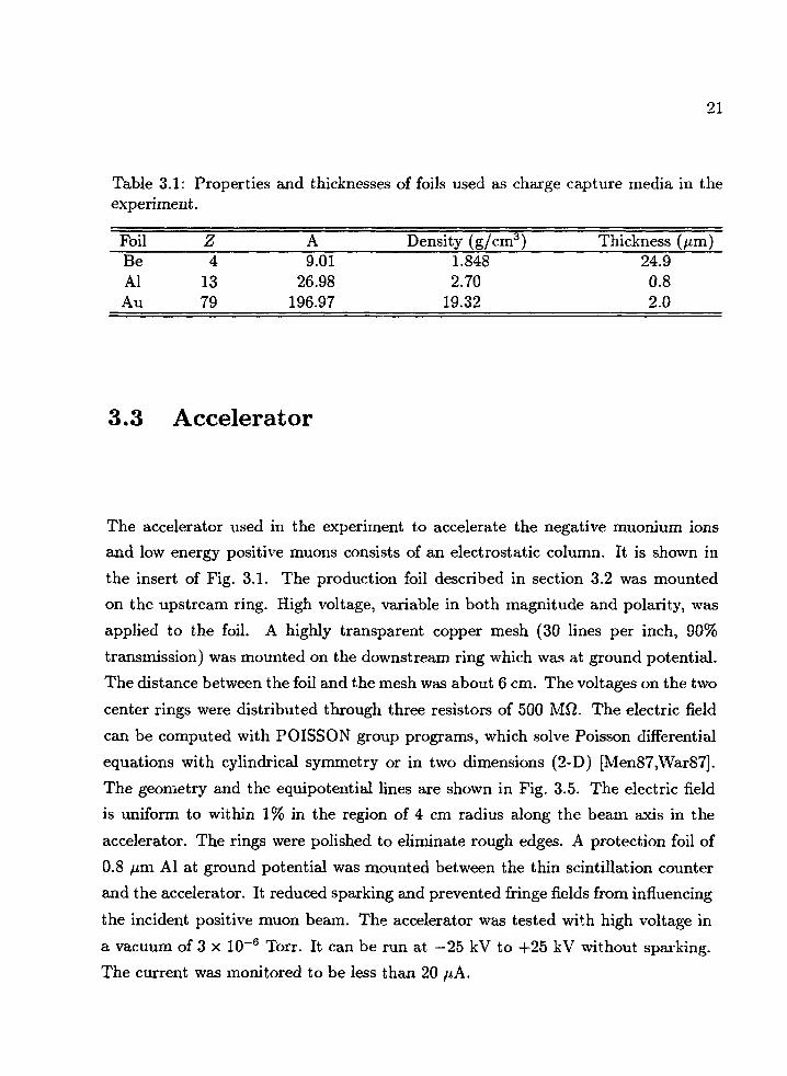
foils of different atomic numbers. Three foils were used in the experiment: beryllium
(Z=4), aluminum (Z=13), and gold (Z=79). Their properties and thicknesses are
listed in Table 3.1. The momentum of the beam was tuned to accommodate the
thicknesses of the different foils. For the Al foil the beam momentum was tuned in
steps of 0.25 MeV/c and the muonium rate was optimized in the straight channel.
For the Be and Au foils, the beam momenta were chosen based on range and energy
loss calculations such that the centroids of the energy distributions of the outgoing
positive muons were close to that for the Al foil.
21
Table 3.1: Properties and thicknesses of foils used as charge capture media in theexperiment.
Foil Z A Density (g/cm3) Thickness9.01 1.848 24.9
26.98 2.70 0.8196.97 19.32 2.0
BeAlAu
41379
3.3 Accelerator
The accelerator used in the experiment to accelerate the negative muonium ions
and low energy positive muons consists of an electrostatic column. It is shown in
the insert of Fig. 3.1. The production foil described in section 3.2 was mounted
on the upstream ring. High voltage, variable in both magnitude and polarity, was
applied to the foil. A highly transparent copper mesh (30 lines per inch, 90%
transmission) was mounted on the downstream ring which was at ground potential.
The distance between the foil and the mesh was about 6 cm. The voltages on the two
center rings were distributed through three resistors of 500 MQ,. The electric field
can be computed with POISSON group programs, which solve Poisson differential
equations with cylindrical symmetry or in two dimensions (2-D) [Men87,War87],
The geometry and the equipotential lines are shown in Fig. 3.5. The electric field
is uniform to within 1% in the region of 4 cm radius along the beam axis in the
accelerator. The rings were polished to eliminate rough edges. A protection foil of
0.8 ^m Al at ground potential was mounted between the thin scintillation counter
and the accelerator. It reduced sparking and prevented fringe fields from influencing
the incident positive muon beam. The accelerator was tested with high voltage in
a vacuum of 3 x 10~6 Torr. It can be run at —25 kV to +25 kV without sparking.
The current was monitored to be less than 20
22
Figure 3.5: Electrostatic accelerator and the eqiaipotential lines computed usingPOISSON group programs.
23
3.4 Magnetic Spectrometer
The bending magnet shown in Fig. 3.1 served as both a charge and a momentum
selector. Particles with the appropriate sign of charge and momentum were deflected
by 60°. Since the intensity of the M~ beam is very small, it is desirable to use a wedge
magnet with a double focusing property [Cam51,Cro51]. TRANSPORT calculations
show that a wedge magnet of "effective" 28 degrees will give the best focusing effect
in both the horizontal and the vertical planes. However, the question arises as to
how to produce an effective field region of 28-degree wedge. This is obviously a
three-dimensional (3-D) problem. In order to answer the question, we again used
the POISSON group programs, which are 2-D programs. The 3-D effect is simulated
with a virtual return path of the field. The studies indicate that the pole pieces and
the coils should also be 28-degree wedges. The pole pieces of an existing H-frame
dipole magnet were modified. New coils were made to accommodate the new pole
pieces. The field of the magnet was mapped. The data show that the wedge angle
of the effective field region is 27.9°, which is in good agreement with the design.
Monte Carlo calculation shows that the magnet has a momentum acceptance of
about 30% (FWHM). The relation between the current (/) and the magnetic field
(B) in the center was measured, and is given by
B(G) = 3.147(A), (3.2)
which is a linear least-squares fit to the data. The magnet was operated at 85 A
providing a central field of 287 G. The bending radius is 22.7 cm.
3.5 Solenoid
The fringe field of a solenoid can provide a focusing effect on a charged particle
beam passing through it. Unlike quadrupole magnets, a solenoid has no defocusing
effect on particle beams. It is preferable to use a solenoid as a focusing element for
a low-energy beam.
The effect of a solenoid on a charged particle can be described as a transforma-
tion matrix [Ban66],
24
'•solenoid —
cos2f
—7^ sin o c o s ^
— sin | cos
2 I2
f sin! cos!
cos2f
fsin^f
s m | ••
cos'f
- sin f cos ! —I sin f cos f
sin ! cos !
f sin ! cos f
cos2f
, (3.3)
where / is the effective length of the solenoid with magnetic field B along its axis,
9 — qBl/cp, c is the speed of light, and q and p are the charge and the momentum
of the particle. The transformation matrix acts on a vector
X =
I \x
x
y(3.4)
specifying the coordinates of the particle, where x and y are the horizontal and
vertical displacements, respectively, x' and y' are the angles of the momentum of
the particle with the beam axis in the local rectangular system. The transformation
matrix can also be written as a product of two matrices
•'-solenoid —
cos I 21,
—^7 sin x cos
0
0
cos!
0
- s i n !
0
0
0
cos!
0
-sin I
0
0
cos!
TTT s m 7721
sin!
cos:
0
021
cos!
sin!
0
cos!! /
(3.5)
The second matrix in Eq. (3.5) represents a simple rotation of coordinates and is
25
insignificant. The first matrix represents focusing in both "horizontal" and "ver-
tical" planes. Since the solenoid is cylindrically symmetric, we consider only the
motion in the "horizontal" plane. Suppose a particle starts from a point located at
a distance l0 from the upstreair end of the solenoid. The initial coordinates of the
particle are
(3.6)
The "image" of the particle is located at a distance /, from the downstream end of
the solenoid. The final coordinates are
(3.7)
They are given by
coscos
We obtain
cosf-^sinf
- 4 sin I
f/•)cos| + f sin|-~
cosf-fsinf
sinXo
Therefore, the condition for point to point focusing is
8 21 0 91 1 9(l0 + li)cos- + _ S i n - - - ^ i s i n - = 0 .
( '
(3.9)
(3.10)
It can be assumed that the spatial distribution of the outgoing beam intensity is
Gaussian on the focal plane
where p is the radius vector in the polar coordinate on the focal plane and a(p) is
approximately proportional to a;,-, which is a function of the momentum, p. There-
fore, the probability for a particle of momentum p to hit a detector of radius r on
26
the focal plane is given by
P(p<r,p) = / / --i—exp—i-gr^7o Jo 27rj2(p) \ 2<r2(p)/
pdpd(j)
1 r2
(3.12)
The width of the distribution depends also on the size of the detector, r. A computer
simulation of the momentum acceptance using MUTRACE is shown in Fig. 3.6. The
1400
tn
Figure 3.6: Momentum acceptance of the solenoid based on MUTRACE calculation.lo = 40 cm, U = 25 cm, B = 713 G, / = 135 cm.
momentum acceptance at p — 2 MeV/c is about 8.5% (FWHM) for a detector of
3.8 cm radius, which is much smaller than the acceptance of the bending magnet.
The peaks at 2 MeV/c and 3.2 MeV/c are relevant to the experiment. In the later
27
stages of the experiment we observed the peak at 2 MeV/c and part of the peak
at 3.2 MeV/c in the time-of-fiight measurements. It is also useful to study the line
shape of the solenoid, since it determines the acceptance of our apparatus. One can
expand <72(p) as a Taylor series in (p — p0) around p0, where <72(p) has its minimum.
Since the first derivative of cr2(p) vanishes at p = p0 and the second derivative is
positive at p = po, we have
a\p) = a\p0) + k(p - po)2 + O((p - po)3), (3-13)
where k > 0.
In general, the phase space of the incident beam to the solenoid is not an erect
ellipsoid. Therefore we can write the expression for <r2(p) as
2, , ( e eh . e\2
a(P) = <7l l(«>s---sm-
n ( o eu . e\ / e 21 . e+2a12 I cos - - — sin - I U- cos - + — sin -
8 21 8\2
- + -s in-J , (3.14)
where &ij are the matrix elements of the phase space. Equations (3.12) and (3.14)
will be used later in the data analysis.
The coils of the solenoid are made of 2.54 cm wide and 50.8 ^m thick Al strips.
They have an inner diameter of 28.7 cm, an outer diameter of 39.1 cm, and are 128.9
cm long. Cooling water flows through two sets of copper tubing between the vacuum
pipe and the coils. The whole solenoid is covered with a cylindrical tube of 0.95
cm thick iron and of 45.8 cm o.d. and the two ends are covered with 0.95 cm thick
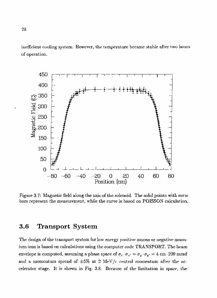
plates of iron, providing a return path for the magnetic field. The field along the
axis was mapped and found to be in good agreement with the POISSON calculation
shown in Fig. 3.7 by a smooth curve. The current density used to produce 380 G
in the measurement was 62.0 A/cm2, while the current density is 59.7 A/cm2 in
the POISSON calculation. The difference is due to the spacing between windings.
The effective length was measured to be 135 cm. The solenoid was operated at
15 A, which gave 712.5 G along the axis. The magnet got hot because of the
28
inefficient cooling system. However, the temperature became stable after two hours
of operation.
-80 -60 -40 -20 0 20 40Position (cm)
60 80
Figure 3.7: Magnetic field along the axis of the solenoid. The solid points with errorbars represent the measurement, while the curve is based on POISSON calculation.
3.6 Transport System
The design of the transport system for low energy positive muons or negative muon-
ium ions is based on calculations using the computer code TRANSPORT. The beam
envelope is computed, assuming a phase space of ax • ax< — ay • ay< — 4 cm • 200 mrad
and a momentum spread of ±5% at 2 MeV/c central momentum after the ac-
celerator stage. It is shown in Fig. 3.8. Because of the limitation in space, the
29
CD
tsi t
15
I 10
»co a.a. ow 2
jQ)
= • . . . I • • • • l . • . • I I0.0 0.5 1.0 1.5 2.0
Z(m)
2.5 3.0
Figure 3.8: Beam envelope of the transport system.
optimum double-focusing condition was not applied. However, the system resultedin a symmetric beam envelope in horizontal and vertical planes. The beam ellipsesat different locations are shown in Fig. 3.9. The size of the beam spot on the mi-crochannel plate is about 4 cm in radius. The transport efficiency of the system isabout 36% as calculated using TURTLE [Bro74]. In the experiment, the solenoidwas set at 712.5 G, which is the highest field one can obtain without over-heatingof the magnet. The field of the bending magnet was first tuned to have maximumtransmission of positive muons. The accelerating voltage was varied to accelerate
30
low energy positive muons to the momentum acceptance of the spectrometer. Neg-
ative muonium ions were studied, by reversing the polarities of the accelerating
voltage and the field in the bending magnet.
500
|
- 5 0 0
"BEAM
! (: LV-BEND
1 1 1 1
>
• MCP
: /
it1I
• i i i
-10 0 10X (cm)
10 0 1 0 - 1 0 0 10X (cm) X (cm)
500
IIE 0
"BEAM
- 5 0 0 ' i i i i I i i i i
;BEND
• i • i • 1 1 •
• MCP
; /
it11
1 1 fl 1
-10 0 10 -10 0 10 -10 0 10
Y (cm) Y (cm) Y (cm)
Figure 3.9: Beam ellipses at different locations of the transport system.
3.7 Detectors and Logic
The detectors used in the experiment are a thin plastic scintillation counter, a
microchannel plate, several thick plastic scintillators and a Nal crystal scintillator.
In order to have a minimum amount of material in the beam, a thin plastic scin-
tillator (NE102A) of 20 Jim. thickness was used as a //+-beam monitor. This detector
31
is essentially identical to the one used in the experiment on formation of muonium
in the 2S state and observation of the Lamb shift transition [BadS4,Woo85]. It is
expected that 670 scintillation photons can be produced by a positive muon of 9.75
MeV/c passing through the scintillator, while only 30 photons will be produced
by a 1 to 40 MeV positron. The scintillation light was transported through four
Lucite light guides to four photomultiplier tubes. These tubes are RCA 8850 type
photomultipliers which are designed for low light level measurement applications.
Since the efficiency of the scintillator for detecting a positron was less than
18%, while the efficiency for a positive muon was about 92% in each phototube, a
three-out-of-four logic, which required that more than two of the four tubes fired
in coincidence, was set up to increase the detection efficiency for positive muons
and, at the same time, to reduce the efficiency for positrons. The logic diagram
is shown in Fig. 3.10. El, E2, E3, and E4 are the signals from the four tubes.
Each signal was amplified and then triggered a leading-edge timing discriminator,
providing pulses of 20 nsec width. The discriminator thresholds were set just below
the single photoelectron peak, in other words, in the noise band. The //3/4 signal
had an efficiency of 97% for positive muons and of 2% for positrons and it was
used as the signature of a positive muon entering the apparatus. This signal was
used to measure the time-of-flight, which will be discussed later in this section, and,
together with the other signals from coincidence levels 1, 2, and 4, was read into
several CAMAC [Clo82] sealers for an efficiency check of the scintillator. It should
be noted that the analog sum of El, E2, E3, and E4 can also be used as a signature
for a positive muon with a properly set discriminator threshold, since a positive
muon gives a much larger pulse height than a positron does.
The Michel energy spectrum of positrons from positive muon decay can be mea-
sured with a Nal(Tl) crystal scintillator. The positrons from positive muon decay
have energies up to 53 MeV with a maximum range of about 5 cm in Nal. The
Nal(Tl) crystal is a cylinder of 25 cm diameter and 25 cm height. It has a photon
yield of about one photon per 25 eV of deposited energy. The scintillation light was
viewed by seven phototubes with the gains adjusted to be equal. Hence, the pulse
height is approximately proportional to the deposited energy [Bir64,Yua6l]. The
32
Amplifiers
El
E2
E4
1?
N
N—k2—
\ j —
Ane
Disc.
Disc.
Disc.
Disc.
K
. Sealers
J[ Sealers
^ Sealers
J Sealers
ilog Sum
Fan.
Fan.
Fan.
Pan.
r " j/4 Y-J. Sealers
- - 2/4 ]H£ Sealers
-- y
" ' 3/4 P ^ Sealers
~~ 4-/4 ) > Sealers
Figure 3.10: Logic diagram for muon counter.
energy resolution was found to be 22%/E1/4 (FWHM) [Hug72], where E is in MeV.
The analysis will be presented in Chapter 5.
A scintillator telescope consisting of two circular plastic scintillators, Tl and T2,
0.5 cm thickness and 6 cm radius, was placed between the beam stop and the Nal
crystal. The telescope subtended a fractional solid angle of 2.9% at the center of the
beam stop in the straight direction. An anti-coincidence counter, A, located above
the beam stop was used to veto signals from cosmic rays. It was a 0.8 cm thick plastic
scintillator and had an area of 30 cmx30 cm. The Nal was also surrounded by four
plastic scintillators, Al, A2, A3, and A4, each of them bent to form a quarter of a
33
circle. Lead bricks surrounded this anti-coincidence shield. EMI 9813B phototubes
were used for these detectors. These scintillation counters had an efficiency of about
95%. A block diagram of the logic for measuring the Michel spectrum is shown in
Fig. 3.11. The analog signal was amplified by a Tennelec TC203BLR amplifier with
Al 1 Disc.
A2 |Pisc.
A3 Disc. J
A1+A2+A3+A4
A4 Disc. —'
Disc.
Tl Disc.
T1«T2«A
T2 1 Disc.
Beam Gate
DelayGate
Amplifier
Nal- Fan. >»qVtSCA TTL/NIM
DelayGate
Sealers
Gate
Analog
Delay
ADC
Figure 3.11: Logic diagram for measuring the Michel spectrum.
a gain of 14.5 and 0.25 /isec shaping. The delayed unipolar output was taken as the
input to a LRS 2259 amplitude-to-digital converter (ADC). The prompt bipolar
output of the amplifier was given to a Canberra single channel analyzer (SCA)
operated in dual discriminator mode, which set a lower level threshold of 0.25 V
34
and an upper level threshold of 10 V. This signal was gated by the scintillator logic
signal together with the beam gate, which represents the macro time structure of
the primary proton beam, to form an interrupt to the CAMAC and a gate of 1 fxsec
for the ADC.
At the end of the 60°-channel, a microchannel plate (MCP) was mounted in the
center of the vacuum chamber. It served as both a beam stop and a detector for
positive muons and negative muonium ions transported through the 60°-channel.
The MCP is a pair of microchannel plates in which the channel axes of the two plates
are tilted by 16° with respect to one another in order to eliminate spurious noise
caused by positive ion feedback [Wiz79]. It is a Chevron CEMA (Model No. 3075)
manufactured by Galileo Electro-Optics Corp. shown in Fig. 3.12. It has an active
diameter of 75 mm. Each channel plate has a bias angle of 8° with respect to the
front surface. The channels have a length to diameter ratio of 90, with a diameter
of 25 Jim and a center to center spacing of 32 /tm, which gives a 55% open area
ratio. A stainless steel disk is mounted at the back of the microchannel plates as
an anode for electrical signal readout. A 95% transparent grounded Cu mesh (20
lines per inch) is mounted in front of the MCP.
The MCP was operated at 815 V per plate with no interplate bias voltage. This
mode of operation helped to discriminate heavy particles, which produce consider-
ably larger pulses, from positrons. The pulse amplitude spectra were taken during
the experiment with a LRS 2259A ADC. The detection efficiency of a MCP has
been studied with H+, He+, and O+ in the energy region of several keV [Gao84]
and found to be (65±10)% [Ort85]. The same efficiency is expected for muons,
although no direct measurement is available.
Two pairs of scintillators Cl, C2 and C3, C4 were mounted, respectively above
and below the MCP to detect the decay positrons from positive muons or negative
muonium ions stopped in the MCP. These scintillators were essentially identical to
the scintillator A described above. They subtended a fractional solid angle of 16.2%
at the MCP. The logic diagram for the scintillator telescopes is shown in Fig. 3.13.
The signature of a positive muon or of a negative muonium ion incident on the
MCP was defined as a delayed coincidence of the signaJ from the MCP and 4.2 /xsec
35
Mesh MCPl MCP2 Anode SCALE
1.02M0 \.02un
1 cm
0.0022/if
Signal
•llkf)
AA/VAW <= +HV
0.0022/if
Figure 3.12: Schematic diagram of the wiring for the MCP detector.
36
Cl Disc.
Sealers
C2 Disc.
Sealers
Beam Gate
. Sealers
rC3 Disc.
Sealers
C4 Disc.
Sealers
C12-C34}*- Sealers
Sealers
(C12+C34)«BEAM
Sealers
Figure 3.13: Logic diagram of the scintillator telescopes for detecting decay posi-trons from MCP.
gate, (C12+C34)-BEAM, shown in Fig. 3.13. This coincidence signal is denoted as
the START to the time-to-digital converters (TDC), shown in Fig. 3.14. One of the
TDC's measured the muon lifetime (LIFE) and the other the time-of-flight (TOF)
of positive muons or negative muonium ions from the muon counter to the MCP.
The delayed (C12+C34)-BEAM signal was used as a stop in the measurement of
muon lifetime, in which aXRS 2228A TDC, modified to have about a 5-^sec range,
was used.
An EG&G TD104 TDC was used for the time-of-flight measurements. The fi3j4
signal was delayed by about 1 /zsec. The time-of-flight was measured in reversed
timing, since the instantaneous counting rate of the MCP is less than 200 sec"1,
which is significantly lower than the instantaneous rate of the ny4 of 2.3xlO6 sec"1.
37
1
(C12+C34)-BEAM
M L r
G.G.
4.2/is
G.G. •
3.4/L4S •
DelayM3/4 ~ /OTN
a
D
L
D
L
- Fan.
- Fan.
STOF
) ]
i—\
>
1 11 LnILjD
Fan. -
G.G.
3.6/j.s
G.G.
3.6/iS
G.G.
3.6/J.S
START
IJ
D
) 1D
L
D
G.G.
170/iS -
START
STOP1
ST0P2
STOP3
)
, TDC- (LIFE)
) PT
TDC(TOF)
Figure 3.14: Logic diagram for muon lifetime and time-of-flight measvirements.
38
The logic shown in Fig. 3.14 was set up in a cascading fashion to allow three stop
signals, STOP1, STOP2, and STOP3, corresponding to three hits in the muon
counter for each MCP signal. This TDC was also modified to have about a l-/isec
full range.
The TDC gains were calibrated with the setup shown in Fig. 3.15. The frequency
FREQUENCY
SYNTHESIZER
RANDOM
PULSER
FREQUENCY
COUNTER
Disc.
Disc.
LOGIC FOR CALIBRATING TDC
\ __J-L
AtD
J '
GateGenerator
STOP
TDC
START
Figure 3.15: Circuit diagram for calibrating TDC's.
synthesizer, a FLUKE 6160A, generates a sine wave of very stable frequency. The
frequency was monitored using a FLUKE 1953A frequency counter/timer. The
width, At, of the gate from the gate generator was adjusted to be close to the
range of the TDC. This gate generator acts as a pileup gate. The random pulser
was a scintillation counter. The START randomly picks up some signals from the
39
frequency synthesizer. The circuit generates a set of peaks in the TDC spectrum
with known distance apart, given by the period of the pulses from the synthesizer.
The centroid of each peak was recorded and fitted to a straight line. The gains of the
LRS 2228A and the EG&G TD104 were found to be 2.5267±0.0008 nsec/channel
and 0.999±0.001 nsec/channel, respectively. The relation between the time-of-flight
and the channel number in the EG&G TD104, obtained using a pulser, is
tTOF(nsec) = 916 - 0.999nTDC ± 20 , (3.15)
where txoF is the time-of-flight of a particle from the muon counter to the MCP
and TITDC is the channel number in the TDC. The 20-nsec uncertainty is due to the
absolute time calibration.
The CAMAC modules, such as sealers, ADC's and TDC's, were all set up in
a single CAMAC crate as shown in Fig. 3.16. The sealers in station 1 were not
gated by any signal to record the total number of counts of the detectors, while the
sealers in station 2 and 3 were gated by the primary proton beam. Therefore, aver-
age rates and instantaneous rates of the detectors could be monitored and recorded.
A pulser running at 104 sec"1 was fed into an ungated sealer channel and a gated
sealer channel for time measurements. A 5-/*sec TDC in station 4 was connected to
measure the muon lifetime. The peak-sensing ADCs in stations 6 and 7 were used
for measurements of pulse amplitude of MCP and Nal, respectively. A l-/zsec TDC
in station 16 was for the time-of-flight measurement. Three of the four channels
were used by STOP1, STOP2, and STOP3. They shared a common start from the
MCP. The interrupt register generated CAMAC interrupts from an external signal,
such as the gated Nal logic signal or the delayed coincidence signal of MCP shown
in Fig. 3.14 as PI. The LAM (look-at-me) grader built at Yale buffers the interrupts
generated by each module, allowing the computer to determine which module needs
service. The crate controller was a Standard Engineering CC-Al. The data were
sent to a PDP-11/34 computer via a CAMAC interface, the branch driver, and the
PDP-11 Unibus. The data acquisition PDP-11/34 computer, manufactured by Dig-
ital Equipment Corporation, is a 16-bit computer and has 124k 16-bit words of core
memory, which is the maximum extensible memory space on this type of machine. It
40
CAMAC CONTROLLER
YALE LAM GRADER
VISUAL BRANCHTERMINATOR
DATAWAY DISPLAY
EG&G IR026 INTERRUPT REGISTER
TDC
TDC
EG&G TD104 TDC, 4 CH, 10 BITS
ADC
ADC
ADC
LRS 2259 ADC, 12 CH, 10 BITS
LRS 2259A ADC, 12 CH, 11 BITS
LRS 2228A TDC, 8 CH, 11 BITS
LRS 2551 SCALER, 12 CH, 24 BITS
LRS 2551 SCALER, 12 CH. 24 BITS
LRS 2551 SCALER, 12 CH, 24 BITS
mw
COC\l
CMCM
wo
a>
COiH
CO
in
00•f-H
CM
o
09
CO
!>-
CD
ID
"*
CO
CM
• - «
Figure 3.16: CAMAC module arrangement in the crate.
41
ran on the RT-11 operating system. The PDP-11 Unibus interconnects the central
processing unit (CPU), the core memory and all the peripherals. There was a DEC
VTlOO terminal with Retro-Graphics support for normal operations, controlling the
experiment and displaying histograms, a DECwriter teletype terminal for logging
messages and printing the on-line analysis data, and a printer for program listings.
Two RK05 disk drives were connected to the computer. One of them served as
the system disk which keeps the RT-11 operating system, the utilities and the data
acquisition programs, the other as the data disk to store the on-line analysis data
and histograms. Two magnetic tape drives were used for recording the raw data
during normal data taking.
The data acquisition program called PION was developed at the University
of Heidelberg. It was written in assembly and FORTRAN languages. The pro-
gram could handle up to 6 LRS sealer modules and 20 programmed-data-transfer
(PDT) parameters when this experiment was conducted. The capability was later
expanded. The sealer modules have to be installed one next to another starting
from station 1, while modules other than sealers can be set up in any order after
the sealer modules. The program read the sealers every second. The readout of
the data from modules other than sealers were requested through interrupt. The
data were then buffered and written to magnetic tape after the buffer was full. The
program also processed the data for on-line histograms. It has some limitation on
on-line processing, though it is adequate for monitoring the experiment. The data
on tape contains the information on when a run was started, the structure of the
event data buffer, the number of parameters, the name of each parameter defined,
the data buffer, the time when the run was stopped, and the sum of the sealer data.
A replay program running on a VAX computer of Digital Equipment Corporation
with a VMS operating system was then developed. It can do essentially all the
data processing tasks that PION can. Q routines developed by the MP-1 group at
LAMPF can also be incorporated in the program which allow much more flexibility
in data manipulation. The data can be transferred directly to the VAX by copying
one record at a time or using the FLX utility on a PDP-11/RSX-11M system to
transfer a RT-11 volume on RK05 disk into a Files-11 volume used on RSX-11M
42
and VMS systems, since there was no RK05 disk drive available on the VAX. All
the data replay was done on the VAX computer.
Chapter 4
Experimental Observations
The primary design consideration of the apparatus was optimization of the signal
rate. The formation of neutral muonium was observed with the Nal detector. As
pointed out in Chapter 2, the electron capture probability is very sensitive to the
velocity of the incident positive muon. In order to maximize the formation fraction
of muonium atoms, the momentum of the incident positive muon beam was tuned by
varying the setting of the SMC. At the optimum momentum of the incident beam,
the formation of the negative muonium ions was observed. The times-of-fiight of
the positive muons and the negative muonium ions through the 60° channel were
measured and fronii these the masses of the particles can be computed. The fact that
the negatively charged particles contain muons was further verified by measuring
both the lifetime of the particles and the characteristic Michel spectrum of the
decay positrons from positive muons. In this chapter, the experimental procedure
and observations will be described.
4.1 Observation of Muonium Formation
The initial running stage of the experiment was a search for neutral muonium atoms
with the Al production foil in place. In order to ensure that the Nal detector located
downstream in the straight channel was working properly, the Michel spectrum of
decay positrons from positive muons was measured by bringing positive muons to
43
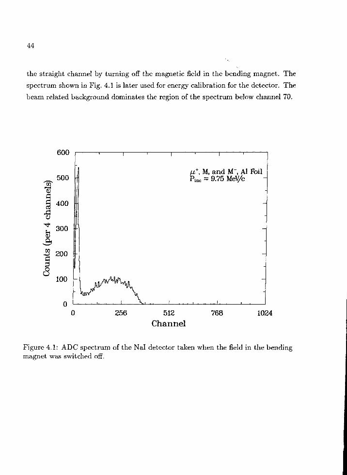
44
the straight channel by turning off the magnetic field in the bending magnet. The
spectrum shown in Fig. 4.1 is later used for energy calibration for the detector. The
beam related background dominates the region of the spectrum below channel 70.
HP
•8
600
500
400
300
I 200g
° 100
0
M+, M, a n d M", Al FoilP i n c = 9.75 MeV/c
0 256 512
Channel768 1024
Figure 4.1: ADC spectrum of the Nal detector taken when the field in the bendingmagnet was switched off.
45
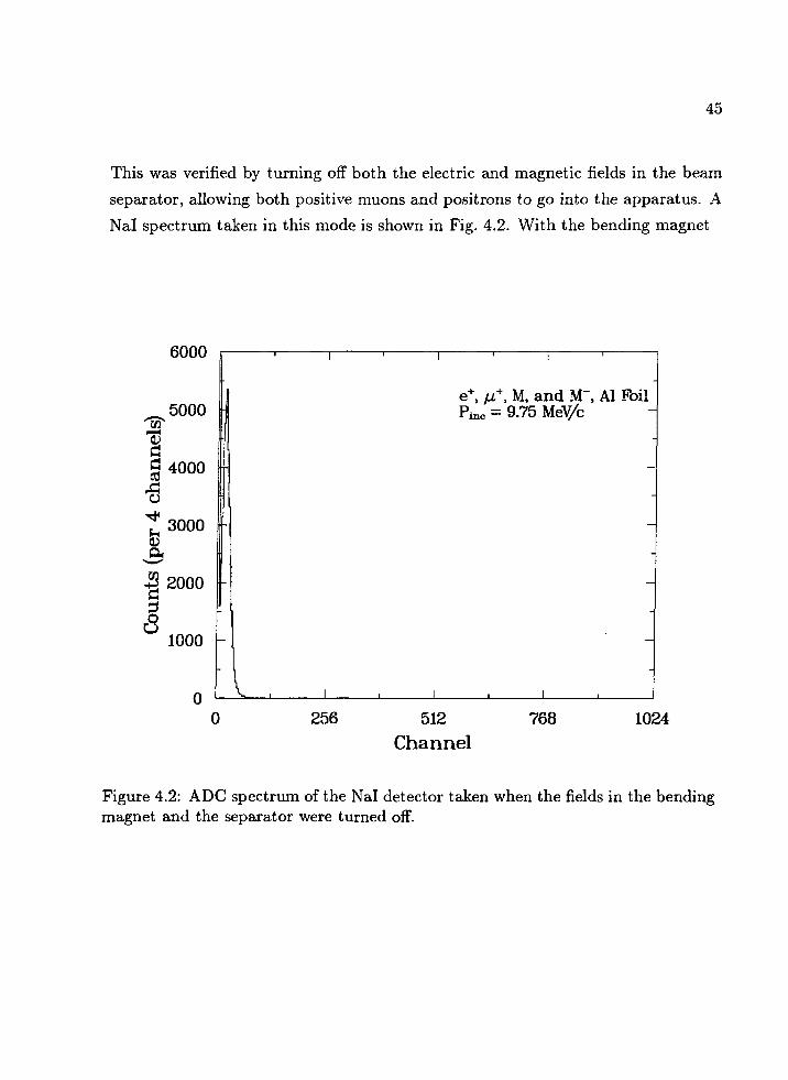
This was verified by turning off both the electric and magnetic fields in the beam
separator, allowing both positive muons and positrons to go into the apparatus. A
Nal spectrum taken in this mode is shown in Fig. 4.2. With the bending magnet
6000
5000
1g 4000I
CO o o o
-| 2000
° 1000
0
e+, JJ,+, M, and M", Al FoilPino = 9.75 M V
0 256 512
Channel768 1024
Figure 4.2: ADC spectrum of the Nal detector taken when the fields in the bendingmagnet and the separator were turned off.
46
fully up (1.1 kG), positive muons were swept out, leaving only neutral muonium
atoms traversing downstream of the bending magnet. The radius of curvature of a
charged particle of 10 MeV/c momentum is about 30 cm in this field. Figure 4.3 is
an ADC spectrum of the Nal detector. The signal rate is much reduced due to the
100
M, Al FoilP i n c = 9.75 MeV/c
.IS nt-. Pi n it.nftVUii « n. /1. I . K , m n.r
256 512Channel
768 1024
Figure 4.3: ADC spectrum of the Nal detector taken when the field in the bendingmagnet was on (1.1 kG).
low formation fraction of muonium atoms. The number of decay positrons detected
in the Nal is determined by setting a window in the ADC spectra from channel
160 to channel 360, which corresponds to 66% of the full Michel spectrum. A flat
background rate based on the data from channel 500 to channel 800 in the ADC
spectrum was subtracted from the windowed data. As is described in Chapter 3,
the acceptance of the Nal is about 2.9% . Therefore, the rate of the muonium atoms
47
at the beam stop was calculated from the number of decay positrons observed. Themomentum setting of the SMC was then tuned in order to optimize this rate. Therates in Nal and projected rates of muonium atoms at the beam stop are listed inTable 4.1. The number of incident positive muons /j,fnc (also in Table 4.1) is given
by_j. \H3/4) gated* ungated yl^Z/AJungated*gated
Vine = ~, ~ T''•ungated ^gated
(4.1)
where t is the experimental running time and the subscripts gated and ungateddenote beam gated and not-beam gated counts respectively. The observed muoniumrates at the beam stop are plotted as solid dots with error bars, in Fig. 4.4, againstthe momentum of the incident positive muon beam. The maximum rate is at
in
b+ 1
Al foili Experiment
— Monte Carlo(at beam stop)
8 8.5 9 9.5 10 10.5 11 11.5 12 12.5 13PM+ (UeV/c)
Figure 4.4: Muonium rate at the beam stop measured at various momenta of theincident positive muon beam.
48
about 9.75 MeV/c. The Monte Carlo simulations using MUTRACE show the same
behavior and are also presented in Fig. 4.4 as a histogram. A similar measurement
was also done with a Au foil. The incident positive muon beam was tuned to 10.67
MeV/c momentum at which the average rate of muons was 140 xlO3 sec""1. The rate
in the Nal was found to be 3.18(18)xlO~7/^+c. The projected rate of muonium
atoms at the beam stop is therefore 1.66(9)xlO~5///^c.
Table 4.1: Average rates of fifnc, rates in Nal and projected rates of muonium atomsat the beam stop.
p^ jj,fnc Rate Rate in Nal Projected Rate at Beam Stop(MeV/c) (103 sec"1)
9.029.499.75
10.0010.25
8010612299117
2.75(28)8.88(37)
10.24(41)9.92(38)8.20(40)
1.44(15)4.64(19)5.35(21)5.18(20)4.29(21)
4.2 Studies of Low Energy Positive Muons
Once the optimum condition for muonium formation was found, the low energy
positive muons could be studied in the 60°-channel. The field of the solenoid was
set to 712.5 G. At this field, the solenoid has a high transmission efficiency for 2
MeV/c particles, as calculated using MUTRACE shown in Fig. 3.6. The positive
muons were used to tune the bending magnet so that the acceptance of the bending
magnet was centered at about 2 MeV/c. A bump was found on a nearly linearly
increasing distribution of the rates in the MCP at 267 G, shown in Fig. 4.5. Fine
tuning was then done around 267 G. The event rates were calculated using the
counts in the regions from channel 288 to 488 in the TDC spectra of the time-of-
flight of the positive muons. The data are shown in Fig. 4.6. The magnetic field
of the bending magnet was set to 267 G for the rest of the measurements based on
these tuning curves.
49
1.2
1 -
0.8 -
0.6 -
0.4
^ 0.2
0160 180 200 220 240 260 280 300 320
Magnet Reid (G)
Figure 4.5: Tuning curve of the bending magnet to maximize the transport efficiencyof the spectrometer.
10
•8
h
1 1
-
-
i
i
i
i
i
i
i
i
i
i
T T ¥ —
—
-
—
1 , 1 , 1 1
2
(S 6
s
1 1
-
1 1
1 ,
1 1
1 ,
1 1
1 ,
1 1
1 ,
1 1 '
1
230 240 250 260 270 280 290Magnetic Field (G)
300
Figure 4.6: Fine tuning curve of the bending magnet to maximize the transportefficiency of the spectrometer. The event rates were calculated using the counts inthe regions from channel 288 to 488 in the TDC spectra of the time-of-flight of thepositive muons.
50
The time-of-flight of positive muons was measured. Figure 4.7 shows the TDC
spectra taken with three stop signals, STOP1, STOP2, and STOP3, described in
the previous chapter for the time-of-flight measurement from the muon counter to
the MCP. Because of the high counting rate in the muon counter, the uncorrelated
events are more probable to be taken as a stop in the lower channels of the first
TDC spectrum. Since STOP2 has to be enabled by STOP1, the probability to
have an uncorrelated event from muon counter in the lower channels of the second
TDC spectrum is reduced. This reduction is even greater in the third TDC spec-
trum using STOP3. This rate effect has been carefully studied by several authors
[Mat71,Low72,Hof82].
As shown in Fig. 3.6, the acceptance of the solenoid reaches a maximum at
many different regions of the particle momentum. Since the momentum acceptance
of the bending magnet is very large (30%), fractions of the positive muons with
high enough momentum in neighboring focusing regions of the solenoid can also
be detected by the MCP. This lower order focusing effect on higher momentum
particles was also observed, as shown in Fig. 4.7 at about channel 620.
The center of the main peak is at channel 444, which corresponds to a time-
of-flight of 472 nsec. The width of about 45 nsec (FWHM) is partly due to the
finite momentum acceptance of the apparatus and partly due to the different path
lengths of the particles in the bending magnet. By scaling down the settings of
the magnetic fields of the bending magnet and the solenoid by a factor (1.415), a
TDC spectrum was taken with zero accelerating voltage. With an extra delay of
128 nsec for the stop signals, a peak was found at channel 382, corresponding to
662 nsec with a width of 50 nsec (FWHM). This confirmed that the time-of-flight
spectrometer was working properly.
Different accelerating voltages on the accelerator were then used to collect pos-
itive muons with different initial kinetic energies. As the accelerating voltage was
increased to 19 kV, the width of the peak became narrower, due to the cutoff of the
energy distribution at zero energy. The TDC spectra taken at 19 kV are shown in
Fig. 4.8.
In the on-line analysis, the counts from channel 388 to 488 in the first TDC
51
400
300
200
100 h
1 '
I. i
fi • i
STOP1ix+, Al FoilHV = 0.0 kV
£ 400
Cd^ 300
T 200
100 I-
3 2000
150
100
50
0256
-. 1-
STOP2/j,+, Al FoilHV = 0.0 kV
STOP3JJ.+, Al FoilHV = 0.0 kV
512 768
Time (channel)
1024
Figure 4.7: TDC spectra for the time-of-flight measurements of positive muons withAl foil and zero accelerating voltage on the accelerator. The timing is reversed.
52
o
fc
6
200
150
100
50
0
100
75
50
25
0
50
40
30
20
10 h
0
, ..A
• J r . .
256
ST0P1/j,\ Al FoilHV = 19.0 kV
ST0P2fx+, Al FoilHV = 19.0 kV
ST0P3Ai+, Al FoilHV = 19.0 kV
512 768 1024
Time (channel)
Figure 4.8: TDC spectra for the time-of-flight measurements of positive muons withAl foil and accelerating voltage of 19 kV on the accelerator. The timing is againreversed.
53
spectrum were taken as candidates for positive muons incident on the MCP. These
rates are designated as the raw rates. The results are listed in Table 4.2, together
with the incident positive muon rates and the interrupt rates. The number of
incident positive muons was calculated according to Eq. (4.1). It should be noted
Table 4.2: Average rates of f<tfnc, interrupt rates and raw rates of positive muonstaken with Al foil at various accelerating voltages. The momentum of the incidentpositive muon beam was 9.75 MeV/c.
AcceleratingVoltage (kV)
21.020.019.018.015.012.06.00.0
-24.2
Htnc Rate(103 sec"1)
132104132133129132121121114
Interrupt Rate(io-7/VL)
43(2)69(2)99(2)
142(2)188(3)192(4)206(5)203(2)205(4)
Raw Rate0-0~7fl4nc)
6(1)18(1)32(1)49(1)62(2)66(2)75(3)68(1)76(3)
that the raw rates contain part of the signals and also some background counts. But
it does give us some idea on how the rates vary at different accelerating voltages.
Because of unequal acceptance of the channel for different accelerating voltages,
this rate dependence on accelerating voltages can not be interpreted directly as an
energy distribution of the positive muons.
As mentioned before, it is interesting to study the behavior of the secondary
beams with foils of different atomic numbers Z. Two other foils were chosen for
these studies, a 25 ^m Be foil of Z=4 and 2 //m Au foil of Z=79. The momentum
of the incident positive muon beam was chosen such that the expected average final
energy of the positive muons coming out the foils is about the same as that for the
Al foil.
For the Be foil, a 12.63 MeV/c incident positive muon beam was used. The data
shown in Table 4.3 have similar behavior as those of the Al foil. The rate foi the
Be foil increases more slowly than that for the Al foil as the accelerating voltage
54
Table 4.3: Average rates of nfnc, interrupt and raw rates of positive muons takenwith Be foil at various accelerating voltages. The momentum of the incident positivemuon beam was 12.63 MeV/c.
AcceleratingVoltage (kV)
21.020.019.017.015.010.06.00.0
/*L Rate(103 sec"1)
125127125110126130128130
Interrupt Rate{IQ-7 / fitic)
33(1)46(1)61(2)
104(2)142(3)163(3)171(4)191(3)
Raw Rate(10~?/lifnc)
5(1)9(1)
13(1)28(1)40(1)43(2)44(2)48(2)
decreases. This indicates that the energy distribution of the positive muons from
Be foil is broader or flatter than that of the Al foil.
The Au data listed in Table 4.4 were taken with a 10.67 MeV/c incident positive
muon beam. We clearly see a maximum rate in the neighborhood of 15 kV to 17.5
Table 4.4: Average rates of /U,y,c, interrupt and raw rates of positive muons takenwith Au foil at various accelerating voltages. The momentum of the incident positivemuon beam was 10.67 MeV/c.
AcceleratingVoltage (kV)
22.520.019.017.515.010.00.0
H?nc Rate(103 sec"1)
147145147146145141145
Interrupt Rate(IO- 7 /A4IC)
15(1)30(1)47(1)67(2)68(2)50(1)43(1)
Raw Rate(10-r//"«tc)
2(1)7(1)
14(1)22(1)21(1)12(1)11(1)
kV in accelerating voltage. Therefore, a narrower energy distribution with the
centroid closer to zero is expected. A more detailed analysis will be presented in
the next chapter.
55
It should be mentioned that the time spectrum of decay positrons from positivemuons and the pulse height spectrum of the MCP were also taken. The timespectrum shown in Fig. 4.9 has three distinct regions. I) The region below channel294 corresponds to uncorrelated events. II) The spike at channels 294 to 300 ispartly due to the decay positrons giving signals in both the MCP and the scintillatortelescope and partly due to cosmic rays. Ill) The region above channel 300 belowchannel 1610 gives the normal time spectrum of muon decay. The cutoff at channel1610 was caused by hardware gate. Therefore the effective window in which thedecay positrons were looked for was 3.3 //sec which accepts 77.9% of all decaypositrons hitting the scintillator telescope.
1600
512 1024 1536Time (channel)
2048
Figure 4.9: TDC spectrum for the lifetime measurements of positive muons withAl foil.
By setting the cuts looking at these three regions separately three pulse heightspectra of the MCP were obtained. The ADC spectra are shown in Fig. 4.10. The
56
512 1024 1536 2048
Channel
Figure 4.10: ADC spectra of the MCP pulse height. Cuts in different regions inFig. 4.9 are used.
57
low energy positive muons give much large pulses than positrons do. This is because
a low energy positive muon generates more secondary electrons than a positron does
when it hits the surface of the microchannel plate.
The events corresponding to the signals below channel 301 in the lifetime spec-
trum give an uncorrelated time-of-flight spectrum. One of such spectrum from
STOP1 is shown in Fig. 4.11. The spectrum has an exponential decay structure
with a time constant of about 0.37to.o2 /^sec, which is in good agreement with the
instantaneous counting rate of 2.3xlO6 sec"1 in the muon counter.
256 512 768
Time (channel)1024
Figure 4.11: Uncorrelated time-of-fBght spectrum. It is taken from STOPl inFig. 4.7 with cuts requiring a count falling below channel 294 in the spectrumshown in Fig. 4.9.
58
4.3 Observation of the Formation of the Negative
Muonium Ion
By reversing the polarity of the bending magnet negative muonium ions were ob-
served. The SMC was again tuned to 9.75 MeV/c subsurface positive muon beam
for the Al production foil. The time-of-flight spectra taken with —17 kV accel-
erating voltage are shown in Fig. 4.12. The center of the peak is at channel 419
corresponding to a time-of-flight of about 497±20 nsec. Taking into account 4-nsec
flight time from the muon counter to the production foil and neglecting the initial
energy of the particle, the mass of the particle is estimated to be 104±8 MeV/c2.
This mass value is consistent with the expected mass of 106.7 MeV/c2 for negative
muonium ion. On the other hand if we take the mass of the ion to be 106.7 MeV/c2,
the initial kinetic energy of the ion can be computed. The length of the accelerator
is 6 cm. The central path length from the downstream end of the accelerator to the
MCP detector is 256 cm. The initial kinetic energy of the ion is estimated to be
0.3 ±1.3 keV. The relatively large error is mainly due to the 20-nsec uncertainty in
the time calibration [see Eq. (3.15)].
The accelerating voltage was then varied, the event rates at different accelerating
voltages are listed in Table 4.5. A maximum was found at about —17.5 kV. The
Table 4.5: Average rates of /j,fnc, interrupt rates, and raw rates of negative muoniumions taken with Al foil at various accelerating voltages. The momentum of theincident positive muon beam was 9.75 MeV/c.
Figure 4.12: Time-of-flight spectra of negative muonium ions taken with Al foil.The momentum of the incident positive muon beam was 9.75 MeV/c. The timingis reversed.
60
width is about 4.5 kV (FWHM) which is close to the acceptance of the apparatus
of 8.5% in momentum. This indicates that the energy distribution of the negative
muonium ion is on the order of a few keV. This narrow distribution can also be
seen in the time-of-flight spectra shown in Fig. 4.12. Another difference oetween
the energy distributions of the positive muons and of the negative muonium ions
is that there is no high energy negative muonium ions. Therefore the second peak
shown up in the positive muon time-of-flight spectra does not exist in the time-of-
flight spectra of the negative muonium ions.
To ensure the peaks are real the spectrometer settings were again scaled down
by a factor (1.415). The accelerating voltage was tuned. In order to take the time-
of-flight spectra, an extra 128 nsec delay was added to the stop signals. A maximum
rate of events at about 8.7 kV confirms that the spectrometer was working. The raw
rates are calculated based on counts in channel 281 to 440 of the first time-of-flight
spectra. They are listed in Table 4.6. These measurements at low channel settings
Table 4.6: Average rates of fj.fnc, interrupt rates, and raw rates of negative muoniumions taken with Al foil at various accelerating voltages. The momentum of theincident positive muon beam was 9.75 MeV/c. The spectrometer settings werescaled down by a factor (1.415).
AcceleratingVoltage (kV)
-8.00-8.50-8.75-9.00-9.50
Htc Rate(103 sec-1)
111131121125128
Interrupt Rate(io-7/i+j
9.1(0.3)10.0(0.4)9.8(0.2)9.7(0.3)8.6(0.3)
Raw Rate(io~7^z^ic)
3.6(0.2)4.4(0.3)4.1(0.1)3.9(0.2)3.4(0.2)
together with the measurements at normal channel settings also enable us to make
better estimate of the initial energy of M~. Since the TDC gain was calibrated very
precisely, from the differences of the times-of-flight at low channel settings and at
normal channel settings the ambiguity in the time calibration can be eliminated
from the estimate of the centroid. A more precise value of 0.16(9) keV is obtained,
which is consistent with the observation of the negative hydrogen ions.
61
The time spectra of the decay positrons were taken at the same time. A typicalnauon lifetime was observed. The spectrum is shown in Fig. 4.13. To further verify
2000
0 512 1024 1536
Time (channel)
2048
Figure 4.13: TDC spectrum for the lifetime measurements of negative muoniumions with Al foil.
62
that the particle contains a muon the Nal detector was moved to the end of the
60°-channel. The characteristic Michel spectrum was observed. The MCP signal
was included in the trigger to further reduce the background. The spectrum is
shown in Fig. 4.14. The ADC gain was recalibrated by bringing the positive muons
into the 60°-channel.
50
<a 4 0
-§ 30C\2COU
3CO
20 -
6 io
00
r
—
i
—i
—
M~, Au Foil
256 512
Channel768 1024
Figure 4.14: Michel spectrum of decay positrons from negative muonium ions.
63
The formation of the negative muonium ions with the Be and Au foils was alsoobserved. The SMC was tuned to a 12.63 MeV/c positive muon beam to accommo-date the thicker Be foil. The rates are listed in Table 4.7. Again a maximum wasfound at about —17.5 kV accelerating voltage. The fraction of formation, however,is reduced by almost a factor of two as compared with that of the Al foil.
Table 4.7: Average rates of nfnc, interrupt rates, and raw rates of negative muoniumions taken with Be foil at various accelerating voltages. The momentum of theincident positive muon beam was 12.63 MeV/c.
AcceleratingVoltage (kV)
-16.00-17.50-18.50-20.00
H?nc Rate(103 sec"1)
136145128133
Interrupt Rate(10~7//i^c)
15(1)18(1)15(1)14(1).
Raw Rate(10-7/l4nc)
3.1(0.3)3.9(0.3)3.8(0.3)3.5(0.3)
Data with the Au foil were taken only in one condition, i.e. at —17.5 kV ac-celerating voltage. The incident positive muon beam was at 10.67 MeV/c with anaverage rate of 146 xlO3 sec"1. The rates are also listed in Table 4.8 for easy com-parison with the other foils. The formation fraction of the negative muonium ionsis comparable with that of the Al foil.
Table 4.8: Average rate of nfnc, interrupt rate, and raw rate of negative muoniumions taken with Au foil. The momentum of the incident positive muon beam was10.67 MeV/c.
There are basically three types of spectra in the experiment, the pulse height spec-
trum of the Nal crystal detector, the time spectrum of the decay positrons, and the
time-of-flight spectrum of the particles from the muon counter to the MCP detector.
The energy distribution of the decay positrons from the positive muons is the char-
acteristic Michel spectrum and was observed using the Nal crystal detector. The
time spectra of the decay positrons give the lifetime of positive muons. A lifetime
of 2.197 ftsec will indicate the existence of the muons. The time-of-flight spectra
will give us some insight into the energy distribution of the particles. In order to
estimate the formation fraction of the negative muonium ions the integrated rates
of the ions in the time-of-flight spectra were computed. The rates of the low energy
positive muons were also obtained. These rates are compared with those of the
Monte Carlo simulations. The computer code for function minimization, MINUIT
[Jam75], was used for most of the least-squares fits. An iteration method was em-
ployed to obtain the undistorted time-of-flight spectra based on the TDC spectra.
The methods of the data analysis will be described in this chapter.
5.1 The Michel Spectrum
The pulse height spectra of the Nal detector were calibrated using a positive muon
beam. It was done by turning off the magnetic field of the bending magnet for the
64
65
Nal detector located at the end of the straight channel. By integrating over the
direction of the positive muon spin 0, the Michel spectrum, Eq. (2.3), becomes
M(x) = 2^/x2 - x20 (3s - 2x2 - xl) , (5.1)
up to a proportional constant, where x = Ee/W, W = 52.831 MeV is the maximum
energy of a positron from positive muon decay at rest, and XQ = 9.67 x 1CT3 is
the normalized electron mass. This expression for the energy distribution of decay
positrons detected by the Nal detector is valid for unpolarized muons. However, it
is also a good approximation for polarized muons, since the Nal detector is at 90°
to the beam direction.
In order to calibrate the spectrum, a linear relation between the energy of the
positron Ee and the pulse height UADC is assumed, i.e.
Ee = Eo + knADC , (5.2)
where EQ is the offset to the energy scale in MeV and k is the energy scale of the
ADC, which has units of MeV/channel. Both Eo and k are fitting parameters to
be computed. Because of the resolution and the finite size of the Nal detector two
corrections are necessary. The effect of the detector resolution can be expressed as
a Gaussian function
( 5 ' 3 >
where a = a/a:1/4 is assumed [Hug72] and a is a fitting parameter. Taking into
account the effect that some of the high energy decay positrons passed through
a corner of the crystal and deposited a fraction of their energy in the crystal, a
function,
h(x) = 1 - sx , (5.4)
is introduced, where s again is a fitting parameter. The parameters a and .s specify
the properties of the Nal detector. The fitting function is therefore
N{z) = N0 ( M(x)g(x, z)h{x)dx + b , (5.5)Jxo
66
where No and b are the only parameters which depend on the running time and the
beam condition of the measurements. By fitting the function (5.5) to the data in
channels 65 to 560, the parameters are found to be
No
b
Eo
k
a
s
= 15.2(5) x 102,
= 0.9(4),
= 3.7(6) MeV,
= 0.142(2) MeV/channel,
= 0.035(4),
= 0.91(2).
(5.6)
The result is shown in Fig. 5.1. The curve is the best fit to the experimental
1000
800 -
600 -
400 -
200 -
0
1 1
'-^ fr
: /
i • J •
Al jn+, 0°-channel
f
V
— i 1— » > . . . . . . . . .
0 20 40 60
ENERGY (MeV)
80
Figure 5.1: Nal spectrum taken with positive muons at the end of the straightchannel for the energy calibration of the detector.
67
data. The first four data points were not used in the fit, since they are background
dominated. Therefore the counts in channel 160 to channel 360 of the ADC spectra
used to estimate the rates of the muonium production constitute 65.9% of the full
spectra. These cuts correspond to an energy window of from 26.4 MeV to 54.8
MeV. By folding in this 65.9% energy cut and the solid angle of 365 msr for the
detector, the muonium rates at the beam stop can be computed and they are shown
in Fig. 4.4. The parameter a gives an expression for the resolution of the detector
22%I'E1'4 (FWHM), where E is in MeV.
It should be noted that the decay positrons were viewed by the Nal detector
through a 0.13 mm Al window at the end of the straight channel, while there was
no special window for decay positrons at the end of the 60°-channel. The decay
positrons had to go through the 1.6 mm Al wall of the vacuum can. Therefore the
Nal detector has to be recalibrated for data taken in the 60°-channel. The same
fitting function as Eq. (5.5) was used. The parameters a and s are fixed to be 0.035
and 0.91 respectively. The fit is shown in Fig. 5.2. The cutoff at 20 MeV is caused
by the threshold of the discriminator. The data point at 20 MeV was not used for
the fit. The parameters are found to be
No = 3.03(7) x 102,
b = 0.5(3),
Eo = 13.5(1.4) MeV, (5.7)
k = 0.121(4) Me V/channel.
The larger offset Eo to the energy scale than that in the straight channel is due to
bigger energy loss of the positron when it passed through the wall of the vacuum
can.
For the data taken with the negative ions the parameters Eo and k are fixed to
be 13.5 and 0.12 respectively given in Eq. (5.7) as well as a and s determined by
the positive muon data taken in the straight channel [Eq. (5.6)]. The fit is shown
in Fig. 5.3. The parameters are found to be
No = 0.68(4) xlO2 ,
b = 1.8(5). (5.8)
68
g
200
150
100
50
n
-
: /
- /
A
i
i
fj.+, 60°-channel
-
->—*^i > •« .»
0 20 40 60 80
ENERGY (MeV)
Figure 5.2: Nal spectrum taken with positive muons at the end of the 60°-channelfor the energy calibration of the detector.
60
20 40 60
ENERGY (MeV)
Figure 5.3: Nal spectrum taken with negative muonium ions at the end of the60°-channel.
69
The x2 is 8 for 13 degrees of freedom. The first data point was not used in the fit.
This good fit indicates that the energy spectrum of the secondary particles from
the negative ions stopped in the MCP is a Michel spectrum. Hence the negative
ion contains a muon.
5.2 Muon Lifetime
The time spectra of the decay positrons from positive muons should have a charac-
teristic of exponential decay. The behavior can be expressed analytically as
f — ) <ft , (5.9)— exp
where UTDC is the channel number of the center of each bin, w is the number of
channels in each bin, and NQ and r are fitting parameters, a least-squares fit has
been performed in which w was taken to be 32. All data taken with low energy
positive muons transported to the end of the 60°-channel are added together. The
data are shown in Fig. 5.4, together with the fitting function (5.9), which is a
least-squares fit to the data from channel 321 to channel 1600. A computed flat
background based on the counts in channels 1 to 160 has been subtracted from the
data prior to the fitting. The parameters are found to be
No - 876(5) x 102,
rM = 870(11) channels, (5.10)
= 2.20(3) //sec ,
where the TDC calibration constant of 2.5267±0.0008 (Usec/channel was used.
The data taken with the negative muonium ions shown in Fig. 5.5 are treated
in the same way. The best fit gives the following values for the parameters
No = 180(2) x 102,
rM- = 856(26) channels, (5.11)
= 2.16(7)/xsec.
70
io4
io3
irv3
lu
11
11
/i
1 , 1
T M = 2.20(3) yusec ;
i 1
11
1 .
i .
i , "
0 512 1024 1536TIME (channel)
2048
Figure 5.4: Time spectrum of the decay positrons from positive muons at the endof the 60°-channel.
104 F
io3 ,192
10s =-
0 512 1024 1536TIME (channel)
2048
Figure 5.5: Time spectrum of the decay positrons from the negative muonium ionsat the end of the 60°-channel.
71
The measured lifetimes of both the low energy positive muons and the negative
muonium ions are in good agreement with the present best value of muon lifetime
of 2.19703(4) (isec [Agu86].
5.3 The Time-of-Flight Spectrum
Because of the high counting rate in the muon counter the TDC spectra for the time-
of-flight measurements are distorted. An earlier stop signal uncorrelated to the start
signal has a higher probability to be recorded in the TDC than a stop signal coming
later. This effect can be seen in Figs. 4.7, 4.8, and 4.12. It is necessary to correct
this rate effect in order to obtain the undistorted time-of-flight distribution, i.e. the
distribution for correlated events.
One way to correct this effect is to accept only those events for which there is no
more than one stop signal in some optimized time window. Since there will be no
second stop signal in this window, the rate effect will be greatly reduced. However
there will be a compromise between the cleanness of the resultant spectrum and
the overall efficiency of the time-of-flight spectrometer, since a wider window will
result in a cleaner spectrum and fewer correlated counts in the spectrum. A time
window, channel 140 to channel 650, is set up to obtain clean time-of-flight spectra.
It requires having one and only one stop signal in this window. The spectra for
low energy positive muons taken at HV=0.0 kV and HV=19.0 kV, and negative
muonium ions at HV= —17.0 kV with an Al foil are shown in Figs. 5.6, 5.7, and 5.8
for comparison with the raw spectra shown in Figs. 4.7, 4.8, and 4.12 respectively.
As pointed out in Chapter 4, the width (45 nsec) of the main peak in the
spectrum shown in Fig. 5.6 taken at HV = 0.0 kV with the Al foil is due to the
momentum acceptance of the spectrometer and the different path lengths of the
particles in the bending magnet. At high accelerating voltage (19.0 kV), very low
energy positive muons were collected and hence the peak in Fig. 5.7 is narrower.
There is a small peak at about channel 620 in both Figs. 5.6 and 5.7, due to the
the solenoid focusing effect at 3.2 MeV/c. Since there are few negative ions with
initial kinetic energies above 5 keV, there is only one peak in Fig. 5.8.
72300
150 200 250 300 350 400 450 500 550 600 650
TIME (channel)
Figure 5.6: Time-of-flight spectrum of positive muons obtained by requiring nomore than one signal falling into a window from channel 140 to channel 650. Theaccelerating voltage was 0.0 kV.
100
150 200 250 300 350 400 450 500 550 600 650
TIME (channel)
Figure 5.7: Time-of-flight spectrum of positive muons obtained by requiring nomore than one signal falling into a window from channel 140 to channel 650. Theaccelerating voltage was 19.0 kV.
73
"C/T
C
I
1
150 200 250 300 350 400 450 500 550 600 650
TIME (channel)
Figure 5.8: Time-of-flight spectrum of negative muonium ions obtained by requiringno more than one signal falling into a window from channel 140 to channel 650. Theaccelerating voltage was —17.0 kV.
Another way to analyze the data is to study the relation between a TDC spec-
trum ^nd a distribution undistorted by uncorrelated events. An undistorted dis-
tribution can be obtained, if one can derive an analytical expression for the TDC
spectrum based on the undistorted distribution. In order to do so we consider the
counting rate of a stop signal R(t) as a function of time. We suppose that the
counting process is purely Poisson. The probability that k stop pulses occur in a
time interval from 0 to t is given by
(5.12)
Therefore the probability that the first stop pulse occurs at time t is the same as
the probability that none occurs in the time interval from 0 to t; i.e.
(f'R(r)dT) , ft vP{k) = {J° y ; exp (- I R{r)dr) .
- f R(r)dr\ . (5.13)
74
Hence the TDC spectrum would be
M(t) = NR(t)exp(- f R(T)dr) , (5.14)
where N is the number of measurements, i.e. the number of start pulses in the TDC.
Let us first consider the spectrum of STOPl in which the first pulse of the stop
counter is recorded. If a start signal is given by a pulse which is uncorrelated to the
stop pulses (call it type I start), the probability density that a stop pulse occurs at
time t is
Pf (t) = Ue~ut , (5.15)
where U is the instantaneous counting rate of the detector used for the stop signal.
If a start signal is given by a pulse which is correlated with one of the pulses in
the stop counter (call it type II start), there are two types of possible stop pulses
in the STOPl spectrum. Let us assume that C(t) is the probability distribution of
the correlated events, which is what we are mostly interested in. The probability
density of having an uncorrelated stop in STOPl spectrum with such a start is
Pfl (t) = Ue'Ui (l - J* C(T)dr) , (5.16)
while the probability density of having a correlated stop with such a start is
if2 (<) = C(t)e-Vt . (5.17)
If we assume N such measurements and that there is one correlated pulse from the
stop counter for each of the Nc measurements (type II start), the TDC spectrum
would be given by
Mi(t) = (N - Nc) Ue~ut + NcUe~Ut (l - f C(r)dr)\ Jo )
+NcC(t)e-Ut . (5.18)
This can also be written as
M,(t) = N (Ue-Ut (l - f C'{T)dr\ + C'(t)e-Ut) , (5.19)
where
C'(t) = §-C(t). (5.20)
75
The equation for M\{t) satisfies the normalization condition
N. (5.21)
Mi(t) gives the ST0P1 TDC spectra. Eq. (5.19) will be used to derive the undis-
torted distribution of the time-of-flight spectrum.
For the sake of completeness we now study the distributions of STOP2 and
STOP3 spectra. STOP2 is not enabled immediately by STOPl, since there is
a delay time T^- It causes an effective dead time of r^- For type I start the
probability density of having a stop signal at time t is
(5.22)[0 otherwise.
For type II start, one of the following three cases can happen.
1. If the pulses taken in STOPl and STOP2 are both uncorrelated with the start
pulse, the probability density of having an uncorrelated stop signal in STOP2
spectrum at time t is
P?1 (*) = C (r2) dr2) dr if t > rd2 , (5.23)
0 otherwise.
2. If the pulse taken in STOPl is correlated with the start pulse, the probability
density of having an uncorrelated stop pulse in STOP2 spectrum at time t is
[ 0 otherwise.
3. If the pulse taken in STOPl is uncorrelated with the start pulse, the proba-
bility density of having a correlated stop pulse in STOP2 spectrum at time t
is
otherwise .(5.25)
76
Therefore the STOP2 spectrum can be expressed as
M2(t) = (N- Nc) i f (t) + Nc (P2C1 (0 + i f 2 (t) + P2
C3 (<)) • (5.26)
Again one has the normalization condition
' M2 (t) dt = N . (5.27)FIn the same fashion one can derive the expression for STOP3 spectrum. We
assume a dead time Tdz due to the fact that STOP3 was not enabled until a time
interval T& after STOP2 was recorded. For type I start one can write down the
probability density of having a stop pulse in STOP3 spectrum at time t as
0
tf t > Td2 + Td3 ,
otherwise .(5.28)
For type II start one of the following four cases can happen.
1. If the pulses taken in STOP1, STOP2, and STOPS spectra are all uncorrelated
with the start pulse, the probability density of having an uncorrelated stop
pulse in STOP3 spectrum at time t is
(5.29)
x(l-f*+Td3C(T4)dT4)dT
0
if t > Td2 + Td3 ,
otherwise .
2. If the pulse taken in STOP1 spectrum is uncorrelated with the start pulse,
while the pulse taken in STOP2 spectrum is correlated with the start pulse, the
probability density of having an uncorrelated stop pulse in STOP3 spectrum
at time t is
(5.30)
0 otherwise .
77
3. If the pulse taken in STOPl spectrum is correlated with the start pulse, while
the pulse taken in STOP2 spectrum is uncorrelated with the start pulse, the
probability density of having an uncorrelated stop pulse in STOP3 spectrum
at time t is
j f » (t) = I U2e'U{t-Td2-Td3) CTd3 (/o -T"2 C fa) drx) dr if t > rd2 + rd3 ,[ 0 otherwise .
(5.31)
4. If the pulses taken in STOPl and STOP2 spectra are both uncorrelated with
the start pulse, the probability density of having a correlated stop pulse in
STOP3 spectrum at time t is
= \ x i1 ~ fr3+rd2 C (r2) dr2) dr3) dr if t > rd2 + rd3 ,
Equation (5.36) is a good approximation of Eq. (5.35) for very small At compared
to the range of the TDC. Therefore we have
JNCft) = l_lUM f Mi(*.-)eut> -NU + UJ2NC(«;)A*J , (5.38)
where Mi{i) is the TDC spectrum of STOP1, N is the total number of measurements
(i.e. the number of start pulses), U is the instantaneous rate in the stop counter
which is on the order of 2.3 x 10⁶ sec"1, and At is taken to be the time interval of
one channel of the TDC, which is about 1 nsec.
For each spectrum N is based on all the counts in the spectrum including over-
flow counts and U is based on the counts in the muon counter and on the beam-gated
running time recorded in the sealers for each run. The origin of the time is taken
to be at channel 130 of the spectrum. A first check of Eq. (5.38) is to apply the
equation to the spectrum for uncorrelated events shown in Fig. 4.11. The result
shown in Fig. 5.9 is satisfactory. The average number of counts is slightly above
zero due to the background. The error bars are computed with error propagation.
Applying Eq. (5.38) to the STOPl spectra shown in Figs. 4.7, 4.8, and 4.12, the
undistorted spectra of the time-of-flight are obtained and shown in Figs. 5.10, 5.11,
and 5.12 respectively as solid dots with error bars. To compare these results with
those obtained earlier with the requirement of having no more than one stop pulse
in a time window, the spectra shown in Figs. 5.6, 5.7, and 5.8 are normalized to
the same peak heights as those obtained using Eq. (5.38) and plotted in Figs. 5.10,
5.11, and 5.12 as histograms. The agreements are excellent.
79
-30650150 200 250 300 350 400 450 500 550 600
TIME (channel)
Figure 5.9: Spectrum for uncorrelated events obtained by applying Eq. (5.38) toFig. 4.11.
J I I I ' I ' I ' I • I " !
1 , 1 , 1 , 1 , 1 , 1 . 1 . 1 . 1
150 200 250 300 350 400 450 500 550 600 650
TIME (channel)
Figure 5.10: Time-of-flight spectrum of positive muons obtained by applying Eq.(5.38) to the STOP1 spectrum shown in Fig. 4.7. The accelerating voltage was 0.0kV. The distribution is plotted as solid points with error bars.
so
"ST
150 200 250 300 350 400 450 500 550 600 650
TIME (channel)
Figure 5.11: Time-of-flight spectrum of positive muons obtained by applying Eq.(5.38) to the STOP1 spectrum shown in Fig. 4.8. The accelerating voltage was 19.0kV. The distribution is plotted as solid points with error bars.
400
-50150 200 250 300 350 400 450 500 550 600 650
TIME (channel)
Figure 5.12: Time-of-flight spectrum of negative muonium ions obtained by applyingEq. (5.38) to the STOP1 spectrum shown in Fig. 4.12. The accelerating voltagewas —17.0 kV. The distribution is plotted as solid points with error bars.
81
Finally, to demonstrate that Eqs. (3.12) and (3.14) can be used to describe the
time-of-flight spectra, an undistorted spectrum taken at HV=—24.2 kV with the
Al foil was obtained. It is shown in Fig. 5.13 as solid points with error bars. The
250 300 350 400 450 500
Time-of-FIight (ns)
550 600
Figure 5.13: Time-of-flight spectrum of positive muons decelerated by —24.2 kV.The smooth curve is a fit to the data using function (5.39).
reason that this spectrum taken with decelerated positive muons is chosen is that
it yields flatter energy distribution than those taken at other accelerating voltages
due to the difference in the distribution in different energy regions. The function
used for the least-squares fit is
fC+lT (5.39)N ( n T D C ) = A f C T P(p < r , p)ds ,Jlc—h
where the integrand P',> < r,p) is given by Eqs. (3.12) and (3.14). /c = 254 cm
is the central path length measured from the downstream mesh of the accelerator
82
to the MCP detector, li = 6.4 cm and lr = 10.4 cm are introduced to account for
the difference in path length due to the 60° bend. Assuming a uniform distribution
within a small angle y/ayi, the average momentum p can be computed by
and
P = 2Pz , (5-41)1 + COSy/022
The parameters I and /,• in Eq. (3.14) are taken to be 135 cm and 25 cm respec-
tively. The parameter r in Eq. (3.12) is 3.8 cm, the radius of the MCP detector.
The continuous curve shown in Fig. 5.13 is the least-squares fit to the data. The
parameters in the fitting are found to be
A = 720(65),
t0 = 892(1),
= 9.85(4) cm, (5.42)
cr12 = -7.99(4) cm,
= 0.854(4).
The numbers are in reasonable agreement with the estimation made independently.
However these results are only approximate, since they depend on the energy and
angular distributions of the positive muons.
5.4 Rates of the Low Energy Positive Muons andthe Negative Muonium Ions
From the undistorted time-of-flight spectra obtained by Eq. (5.38), the number of
positive muons and negative muonium ions stopped at the MCP detector can be
computed. The spectra can be divided into two regions. The number of counts was
computed by integrating each spectrum over time from channel 339 to channel 538.
A flat background computed by integrating the spectrum over time from channel
141 to channel 338 was subtracted from the spectrum.
S3
The counting rates of the scintillator telescopes at various accelerating voltages
with the Al foil are listed in Table 5.1 together with the projected rates at the focal
plane where the MCP detector was located. The projected rates are computed by
Table 5.1: Average rates of /i£c, telescope rates, and projected rates of low energypositive muons at focal plane taken with Al foil at various accelerating voltages.The momentum of the incident positive muon beam was 9.75 MeV/c.
taking into account the detection efficiency of the scintillator telescopes (90%), the
time window of the telescopes (3.3 fisec, 77.9%), the fractional solid angle subtended
by the telescopes (16.2%), and the detection efficiency of the MCP detector (65%).
The central momentum of the incident positive muon beam was 9.75 MeV/c.
The results of the measurements on the low energy positive muons performed
with the Be foil and the Au foil are listed in Tables 5.2 and 5.3 respectively. The
Be data were taken with a 12.63 MeV/c incident positive muon beam, while a 10.67
MeV/c positive muon beam was used for the Au foil.
The data taken with the negative muonium ions are analyzed using the same
method as for positive muons. Table 5.4 lists the rates of the negative muonium
ions at various accelerating voltages with the Al foil. The results for data taken at
low spectrometer settings are also given here in Table 5.5. Because of different time-
of-flight and of an extra 128-nsec delay for the stop signal the time window used
here is from channel 231 to channel 431. The background levels are estimated based
on the counts in the region from channel 141 to channel 230. These background
84
Table 5.2: Average rates of jifnc, telescope rates, and projected rates of low energypositive muons at focal plane taken with Be foil at various accelerating voltages.The momentum of the incident positive muon beam was 12.63 MeV/c.
Table 5.3: Average rates of /z+c, telescope rates, and projected rates of low energypositive muons at focal plane taken with Au foil at various accelerating voltages.The momentum of the incident positive muon beam was 10.67 MeV/c.
Table 5.4: Average rates of fj.fnc, telescope rates, and projected rates of negativemuonium ions at focal plane taken with Al foil at various accelerating voltages.The momentum of the incident positive muon beam was 9.75 MeV/c.
Table 5.5: Average rates of fifnc, telescope rates, and projected rates of negativemuonium ions at focal plane taken with Al foil at various accelerating voltages. Themomentum of the incident positive muon beam was 9.75 MeV/c. The spectrometerfields were scaled down by a factor (1.415).
Rate at Focal Plane(10~6/^+c)4.11(0.62)5.61(0.55)6.06(0.67)5.62(0.32)5.42(0.55)5.45(0.55)
86
levels were subtracted from the final results. An incident positive muon beam of
9.75 MeV/c momentum was used for these measurements.
The results on the negative muonium ions measured with the Be and Au foils
are listed in Tables 5.6 and 5.7 respectively. The momenta of the incident positive
muon beam were 12.63 MeV/c for the Be foil and 10.67 MeV/c for the Au foil.
Table 5.6: Average rates of fxfnc, telescope rates, and projected rates of negativemuonium ions at focal plane taken with Be foil at various accelerating voltages.The momentum of the incident positive muon beam was 12.63 MeV/c.
Accelerating fifnc Rate Telescope Rate Rate at Focal PlaneVoltage (kV) (103 sec"1) (10~7'/njc) t
Table 5.7: Average rate of /x+,c, telescope rate, and projected rate of negative mu-onium ions at focal plane taken with Au foil. The accelerating voltage on theaccelerator was —17.5 kV. The momentum of the incident positive muon beam was10.67 MeV/c.
Because of the complicated nature of the transport system employed in the experi-
ment it is desirable to have a Monte Carlo simulation for the system. A Monte Carlo
computer code MUTRACE was, therefore, developed for this purpose. Its physical
principles are described in Appendix A. The program simulates the processes of
energy loss and straggling of positive muons and charge capture by positive muons
87
based on the data from hydrogen and of multiple scattering. It can also be used as
a ray-tracing program for transport system. The main objective is to reproduce the
experimental data using the simulation code. By comparison between the results
from simulations and the results from experiment one can gain some understanding
of the processes.
The phase space of the incident positive muon beam is described by
-3.0 cm
-0.029
-2.3 cm
-0.095
- 5 %
< x <
<x'<
<y<
<y'<
<s<
3.0 cm,
0.029,
2.3 cm,
0.095,
5%,
(5.43)
where x and y are the horizontal and vertical displacements respectively, x' and y'
are the tangents of the angles of the momentum of a particle with the beam axis in
the local rectangular system, and 6 = (p — po)/po represents the fractional deviation
of the momentum p of the particle from the central momentum po of the beam.
The experimental data for muonium production are easier to interpret than
those of the low energy positive muons and the negative muonium ions, since the
later were taken with more complicated channel. Therefore it is natural to study
the muonium production first using the MUTRACE code. The results have been
shown in Fig. 4.4 as a histogram, where a 0.8 //m Al foil was used as the production
foil. The agreement is very good. The Monte Carlo simulations also give predicted
muonium rates at the Al foil, which are shown in Fig. 5.14. Fig. 5.14 shows that the
muonium formation probability is slightly less than 1%. As mentioned in Chapter
4 a measurement to observe the muonium formation with the Au foil gives a rate of
1.66(9)xlO~5//xfnc at the beam stop. The Monte Carlo simulation predicts-a rate of
1.33 xlO~51fifnc at the beam stop and the muonium formation probability of 1.8%
at the foil. The fact that the rate at the beam stop for the Au foil is lower than
that for the Al foil, while the formation fraction for the Au foil is higher than that
for the Al foil is due to a wider angular distribution of the muonium atoms from
the Au foil. We will discuss this effect in more detail later.
88
8.5 9 9.5 10 10.5 11 11.5 12 12.5 13
Figure 5.14: Muonium rates at the production foil predicted by Monte Carlo simu-lation with various momenta of the incident positive muon beam. The productionfoil was 0.8 /zm Al.
The results of Monte Carlo calculations of the low energy positive muons cor-
responding to the data listed in Tables 5.1, 5.2, and 5.3 taken at the end of the
60°-channel can be generated. These are shown in Fig. 5.15. The solid points with
error bars represent the experimental data listed in Table 5.1, 5.2, and 5.3. The
simulations were performed in 1 kV steps and plotted as histograms. They agree
with the experimental data better than a factor of two.
The energy distributions of the positive muons exiting the production foils are
obtained by Monte Carlo simulations. The simulations are based on the experi-
mental running conditions in which the central momenta of the incident positive
muon beam are 9.75 MeV/c for the Al foil, 12.63 MeV/c for the Be foil, and 10.67
MeV/c for the Au foil, respectively. They are shown in Fig. 5.16. The distribution
89
I
inci
150
120
90
60
30
0
100
80
60
40
20
(b) Be
-
foil
i—
r*
• ' i • • • •
•
i > 1 i i i i
« f_n f
-j
-
0
> ' > • i • > ' •• i
(c) Au foil
25 20 15 10
,m< , i • , , , i i • i i i i , i i i , . i ,
Accelerating Voltage (kV)
Figure 5.15: Low energy positive muon rates at the MCP detector with variousaccelerating voltages.
90
o
8.m0Onui
2000
1600
1200
800
400
0
1000
800
600 -
(c) Au foil _
200 400 600 800 1000
(keV)
Figure 5.16: Energy distributions of outgoing positive muons from (a) Al foil, (b)Be foil, and (c) Au foil calculated with the Monte Carlo code.
91
for the Be foil is peaked at higher energy than those for the Al and Au foils and is
also wider. The distribution for the Au foil however is peaked at lower energy than
those others. These characteristics confirm the observation made in Chapter 4.
The process of producing the negative muonium ions can also be simulated
using the MUTRACE code. Again an incident positive muon beam of 9.75 MeV/c
momentum was used for the Al foil. The results of the simulations are shown in
Fig. 5.17 as a histogram. The solid points with error bars in the figure are taken
from Table 5.4. The fact that the width of the distribution (4.5 kV FWHM) is
comparable to the acceptance of the channel suggests that the energy distribution
of the negative muonium ions is narrow (< 4.5 keV FWHM). The results of the
25
20
15
10
* 5
0
Alfoil=9.75 MeV/cExperiment
— Monte Carlo
-12 -14 -16 -18 -20Accelerating Voltage (kV)
-22
Figure 5.17: Rates of negative muonium ions at focal plane with Al foil. Thehistogram represents the Monte Carlo simulation.
92
3
12
10
8
ft 6
* A
I
0
Be foilPinC=12.63 MeV/c£ Experiment
— Monte Carlo
-12 -14 -16 -18 -20Accelerating Voltage (kV)
-22
Figure 5.18: Rate of negative muonium ions at focal plane with Be foil. Thehistogram represents the Monte Carlo simulation.
simulations for the Be foil are shown in Fig. 5.18 as a histogram. The momentum of
the incident positive muon beam was 12.63 MeV/c for the Be foil. The experimental
data listed in Table 5.6 are also shown in the figure as solid points with error bars.
Monte Carlo simulation also gives the rate at the focal plane for the Au foil with a
10.67 MeV/c incident positive muon momentum. The rate is 18.8xlO~6/^inc which
is also in good agreement with the measured rate of 14.6(1.3)xlO~6/fifnc listed in
Table 5.7.
Based on these simulations the projected formation fractions of negative mu-
onium ions at the production foils can be obtained. They are listed in Table 5.8
together with some of the relevant experimental data.
The results for the negative muonium ions can be explained qualitatively as
93
Table 5.8: Projected formation fractions of the negative muonium ion at productionfoils.
Foil nfne M~ Rate at Focal M~ Formationthick. diam. />„+ rate Plane (10-5/^£e) Probability (10-4//*,te)
follows. The energy distribution of the outgoing particles from the Be foil is peaked
at higher energy than for the Al and Au foils. Therefore the stopping density of
positive muons at the surface of the foil is relatively low and hence the formation
fraction of the negative muonium ions is lower. The energy distribution of the
outgoing particles from the Au foil is peaked at lower energy and hence the formation
fraction of the negative muonium ions is higher. Another interesting feature of the
results in Table 5.8 is tha t the collection efficiency of the negative muonium ions,
defined as the ratio of the rate at focal plane to the formation fraction, is not the
same for these different foils. This is due to the fact tha t the angular distribution of
outgoing particles from a foil with larger atomic number Z is expected to be wider
than that from a foil with smaller atomic number due to the multiple scattering,
as indicated in the Monte Carlo simulations. The angular distributions of the
outgoing particles from Monte Carlo simulations are shown in Figs. 5.19, 5.20, and
5.21, respectively.
Finally, it should be mentioned that the Monte Carlo code, MUTRACE, is
also capable of computing the time-of-fiight of the particles. The result of one
such simulation is shown in Fig. 5.22(a). The simulation is performed under the
condition in which the spectrum shown in Fig. 5.10 was taken, i.e. the production
foil is an Al foil, the momentum of the incident positive muon beam is 9.75 MeV/c ,
the accelerating voltage is 0.0 kV, and the bending magnet is set to accept positively
charged particles. The data shown in Fig. 5.10 is plotted again in Fig. 5.22(b). The
time axis has been reversed so that the physical time is from left to right. In both
of these plots the main peak at about 470 nsec corresponds to about 2 MeV/c in
94
8000 -i 1 1 1—i—I 1 1—i 1—i—I—i—I—i—1 r
II
0.00
ar<g> -• 10.6°
i , i , i . i , j ,
15
10
5
n
1 1 ' 1
- X
, 1 , 1
s
• i '
i
i • i <
(b)<T<6
^ ^ - _
1
M
1 1 '
29.4° "
-
-
0 10 20 30 40 50 60 70 80 90
6 (degrees)
Figure 5.19: Angular distributions of (a) / i+ , (b) M, and (c) M coming out ofAl foil. The momentum of the incident positive muon beam was centered at 9.75MeV/c.
95
I 0.60
0.45
0.30
0.15
0.00
(b)M= 16.3°
i , i
i • i • i • i ' i • i • i • r
(c)M-cr<fl> = 16.0°
i . i i i _,- i i i , i
0 10 20 30 40 50 60 70 80 90
9 (degrees)
Figure 5.20: Angular distributions of (a) fj,+, (b) M, and (c) M~ coming out ofBe foil. The momentum of the incident positive muon beam was centered at 12.63MeV/c.
96
g
Ia
, i , , i , , i , , , i
16
12
8
0
0
i • r ^ i ' i ' i ' I r i r
(b)M= 52.9°
, i , i , i i t , i , i , i , i
, , , 1 , 1 , 1 , 1 . 1
0 10 20 30 40 50 60 70 80 90
6 (degrees)
Figure 5.21: Angular distributions of (a) fx+, (b) M, and (c) M coming out ofAu foil. The momentum of the incident positive muon beam was centered at 10.67MeV/c.
97
momentum and the small peak at about 300 nsec, which is also due to the focusingeffect of the solenoid, corresponds to 3.2 MeV/c (see Fig. 3.6). The momentum ofthe particle is first selected by the bending magnet and thus only part of the 3.2MeV/c peak can be seen in the spectra.
6
900
800
700
600
500
400
300
200
100
0
900
800
700
600
500
400
300
200
100
0
i , i i
(a) Al foil, /J.+H V = 0.0 kVMonte Carlo
i .
(b) Al foil, M+
HV = 0.0 kVExperiment
200 300 400 500 600
Time (ns)
700 800
Figure 5.22: Time-of-flight spectra of positive muons, (a) Monte Carlo, (b) mea-surement.
Chapter 6
Summary and Discussion
The negative muonium ion M~ (n+e~e~) has been produced and observed for the
first time. The ion was produced in a beam-foil experiment in which a subsurface
positive muon beam of about 10 MeV/c momentum passed through a thin metal
foil. The mass or the initial energy of the negative muonium ion was obtained by a
time-of-flight technique. The mass of the ion is found to be 104±8 MeV/c2 in good
agreement with the expected value of 106.7 MeV/c2 for M~. The initial kinetic
energy of the ion is in the vicinity of 0.16(9) keV. This is consistent with the proton
data and the velocity scaling rule. The lifetime of the ion is determined by the
lifetime of the muon. The decay process was also observed in the experiment by
measuring the energy and time spectra of the decay positrons.
The observed rate of the negative muonium ion at the spectrometer focal plane
is about 10~5/fj,fnc or 1.4 sec"1 (average). The production foils were placed in
moderately good vacuum (3x 10~6 Torr) and the last several atomic layers of the foils
are believed to play an important role in charge capture processes. The formation
fraction of the negative ions is expected to be the same for all foils. The slight
difference in rates for Al, Be, and Au foils is likely caused by the different incident
beam conditions and the range of the positive muons in the different foils.
The positive muons of a few keV to 20 keV coming out of the foils were studied.
A rate of 1.5 x 10~4/fifnc or 20 sec"1 was observed with an acceptance of 4.5 keV
(FWHM).
98
99
A Monte Carlo computer code, MUTRACE, was developed for this experiment
(see Appendix A). It can reproduce essentially all our experimental data within
a factor of two. The simulations were of substantial help in understanding the
experimental data. The conversion probabilities for the M~ at the foils are about
10~4/^+jC. The differences in M~ rates for different foils are also demonstrated
in the Monte Carlo simulation. From a careful study of the energy and angular
distributions of the particles leaving the foils, these differences can be understood
in terms of the different stopping distributions of the positive muons for different
foils. Studies of the low energy positive muons leaving the foils indicate that the
dE/dx is larger for high-Z material and the angular distribution is also wider.
These are in agreement with general expectations.
The negative muonium ion itself is a very interesting system. A beam of such
ions is now available for spectroscopy and collision studies. An interesting question
to answer experimentally is whether the ions are polarized. In the M~ 1So ground
state no depolarization will occur, but if muonium is formed in a first single e~
capture process, the fi+ can be partially depolarized before the second e~ capture
occurs.
Since the M~ is a charged particle, a beam of neutral muonium atoms can be
generated from an M~ beam. The muonium beam would be useful for measure-
ments of the Lamb shift of the muonium in the n = 2 state [Ora84,Bad84] and
an experimental search for spontaneous conversion of muonium to antimuonium
[Ni87]. Recently, advances have been made on a more intense muonium source in
the thermal energy region [Mil86,Bee86]. This thermal muonium source would be
very useful for the future experimental search for muonium to antimuonium conver-
sion. However at present the fast muonium remains the practical source of muonium
for a Lamb shift measurement. Therefore more careful studies of a fast muonium
source would be beneficial for future Lamb shift experiments.
In the past it was often assumed that the angular distribution of the muon-
ium atoms leaving a foil is isotropic because of a lack of experimental information.
The Monte Carlo simulations developed for this experiment show that the angu-
lar distribution of the muonium atoms is considerably wider than that of positive
100
muons, since the muonium atoms have lower energy than do the positive muons.
One might be able to take advantage of this characteristics of the angular distri-
butions for Lamb shift experiments by using muonium atoms that are produced
at an angle to the beam axis. An improvement on signal to background ratio of
a factor of 30 to 95 can be achieved without much loss of signal rate (a factor of
two at 30°), assuming that the 2S muonium atoms have the same distribution as
the muonium atoms in all states. An improvement on Lamb shift measurement is
therefore feasible with the apparatus used in the previous Lamb shift experiment.
A detailed analysis will be given in Appendix A.
Although the present beam intensity for M~ is small (~ 1.4 sec"1 average),
increases of up to a factor of 10 could be achieved by optimizing the incident / i+
channel and the accelerator-spectrometer arrangement. It is well known that the
charge capture cross sections are larger for alkali metal vapors and alkali metal
coated targets. One would expect a factor of 10 or more increase in formation of
the negative muonium ions using such targets [Ehl80].
Positive muons of a few keV kinetic energy can also be utilized for making M(2S).
One of the effective ways to produce H(2S) is the following process:
H+ + Cs -> H(2S) + Cs+ (6.1)
The cross section of this process is measured to be 10~15 ~ 10~14 cm2 in the range
from 5 to 10 keV kinetic energies of the incident H+ [Sel67]. With the current
setup a M(2S) beam may be produced using the low energy positive muons. The
intensity of this M(2S) beam would be about 0.02 s"1, using a Cs vapor target
of 1011 atoms/cm2, which is about an order of magnitude lower than that in the
previous measurements of the muonium Lamb shift [Bad84]. Positive muons of even
lower energies (< 10 eV) emitted from LiF surface have been observed [Har86].
Unfortunately the intensity was also low (~ \0~7fnfnc). A more intense source of
low energy positive muons with small phase space is needed for a dramatic increase
in intensity of M(2S).
Appendix A
MUTRACE
A.I Introduction
Fast muonium (M or fi+e~) has been utilized in several experiments recently. Be-
cause of absence of the size effect of the nucleus, muonium has become an ideal
system for testing Quantum Electrodynamics. The Lamb shift of muonium atoms
in the n = 2 state has been measured [Ora84,Ba.d84], although improvements on
the experimental precision are necessary for a sensitive test of the theory. A triple
coincidence technique was used in these measurements. It first required a hit in the
muon counter, subsequently a count in the Lyman-a detector, and then a hit in
the microchannel plate (MCP). The timing of the signals depends on the time-of-
flight of the muonium atoms in the 2S state. Thus some knowledge of the energy
distribution of the muonium atoms is needed. A recent experimental search for
muonium to anti-muonium (M or fJ.~e+) conversion gives a new upper limit on the
branching ratio of the process [Ni87], which provides another way of testing the
standard theory of the electroweak interaction [Gla61,Sal68,Wei67]. The signature
of an anti-muonium atom is the detection of Ka and La x-rays from \i~ being cap-
tured by a high Z atom and a hit in a microchannel plate from secondary electrons
created by the anti-muonium atom hitting the stopping target. Therefore the de-
tection probability of such an event is dependent on the time-of-flight of muonium
and anti-muonium atoms in the region of very low magnetic field. The ability to
101
102
compute the time-of-flight of muonium or anti-muonium atom was found to be very
helpful in the data analysis. The muoniurn atoms with kinetic energy of several
keV can be produced by a beam-foil method with a positive muon beam in vacuum
environment [B0I8I]. The processes involved are the energy loss of positive muons,
multiple scattering of positive muons by target atoms and charge exchange between
projectile and the target atoms. The mechanism of the processes are not fully un-
derstood especially in the intermediate energy region. However experimental data
from hydrogen, with reasonable accuracy, is available. Computer simulation of these
processes on phenomenological basis is therefore feasible. The formation of nega-
tive muonium ion (M~ or ^+e~e~, sometimes denoted as Mu") by double charge
capture was also observed [Kua87]. It is very desirable to have a Monte Carlo type
of computer simulation for helping us to analyze the data and to design new ex-
periments. The physical principles of the simulation will be described in sections
A.2, A.3, A.4, and A.5. In section A.6 some results will be presented and will be
compared with experimental data. Finally, the application of the results will be
discussed.
A.2 Energy Loss and Range of Positive Muons
The stopping power of positive muons depends significantly on their velocity. The
theory of energy loss at high velocity, i.e. v ^> Z2^ac with v being the velocity of
the projectile, Z the atomic number of the target material, and a the fine structure
constant, is well established. The inelastic collisions of positive muuns with atoms
can be described by Bethe's formula [Fan63]
dx J H rnev2 \ \ I } V--^j Z 2 )
where p = v/c, me is the electron mass, v is the velocity of the projectile, N is the
density of atoms, I is the mean excitation energy which is denned as a logarith-
mic mean over the excitation energies En weighted according to the corresponding
oscillator strengths fn:
^ , (A.2)
103
and CJZ and S2 represent the so called "inner shell corrections" and "density effect
correction", respectively.
The energy loss in the low energy region (v < ac) is evaluated using the Thomas-
Fermi model of atom [Lin61],
\ UX J £ M -j- 2 / J ' ) OCC
where ao = %2/mee2 is the Bohr radius of hydrogen atom.
The mechanism of energy loss in the intermediate region (v ~ ac), where the
charge exchange processes are favorable, is not well understood. The energy loss in
this region is bridged by [Var70]
(A.4)
Equations (A.I) and (A.3) tell us that the energy loss in both high and low
energy regions depends mainly on the velocity of the projectile. We thus make a
further assumption that dE/dx is the same for protons as for positive muons at
equal velocity. The same methods as used previously [Bol82] are adopted in energy
loss calculation. The data of the energy loss and range of hydrogen [And77] are
used in the simulations. Bragg's additivity rule is employed in computing the range
for compounds, although the rule may not hold exactly at 10% level [Par63,Sau65].
The projected path length is calculated based upon the formulae given by Schi0tt
[Sch66]. The ratio of the projected path length to the total path length is indepen-
dent of material. A Gaussian straggling of 10% of the total path length is assumed
in the range calculation.
A.3 Multiple Scattering
The multiple scattering of a heavy particle in matter is well described by Moliere's
theory [Mol47,Mol48]. The distribution is characterized by two parameters, the
unit probability angle Xc and the screening angle Xa- The detailed derivation is
given by Bethe [Bet53].
104
The number of positive muons in the angular interval d9 after traversing a
thickness / is
^ r ( ! * ) ( ] ( \)) (A.5)Xc
J0 \ Xc
c2^ (A.6)
where Ni is the number of scattering atoms of the ith. species per cm3, Z{ is the
atomic number of the ith species in the material, p and v are the momentum
and velocity of the positive muon, JQ{X) is Bessel function of first kind, and the
parameter b is defined as
6 = l n % + l - 2 C , (A.8)
xlwhere C = 0.577 • • • is Euler's constant.
By averaging over different constituencies, the parameter \a can be written as
Xa = exP (^Exl (lnx« - ~ ) ) • (A.9)
Based on the Thomas-Fermi potential, Moliere gave a formula for Xai
Xa,=Xoi(l-13 +3.76a;2) , (
(A.ll)
a'i = Zie2/hv . (A. 12)
The Thomas-Fermi model is not suitable for low-Z substances [Han51]. A more
precise expression for Xai m a v be obtained using atomic screening functions [Sal87].
However the approximation is sufficient for our purposes.
The second term in Eq. (A.9) is the correction of the scattering of the atomic
electrons. The explicit, expression for the parameter Z?, is given by Fano [Fan54]
A = In (l l30Zf
105
where —u,nt can be calculated using the incoherent scattering functions. The typical
value for — u,n, is about 5.
By defining a new parameter B as
B-\v.B = b, (A.14)
the projected distribution (A.5) can be expanded as
Selected values of functions /(0)(tf), /(1)(tf), and /(2)(??) are tabulated in Bethe's
paper [Bet53].
The theory is considered to be good for B > 4.5 and xl/xl > 2 0 [Mol47,Mol48].
The scatterers considered in our simulations are mylar (C5H4O2), scintillator (CH),
beryllium (Be), aluminum (Al), and gold (Au) foils. The typical average momentum
of the positive muon beam is about 6.5 MeV/c. The values of B and Xc/xl f° r 6-5
MeV/c positive muon in these substances are listed in Table A.I.
Table A.I: Typical B and xl/xl values for the substances used in the simulations.
MaterialMylar
ScintillatorBerylliumAluminum
Gold
Thickness (^m)1.5
19.124.90.82.0
B7.3
10.111.65.95.4
xllxi231
283910755
7147
106
A.4 Charge Exchange
The secondary beam from a thin metal foil consists mainly of positive muons (//+),
muonium atoms (M or ft+e~) and negative muonium ions (M~ or fi+e~e~). Much
experimental and theoretical work has been done on hydrogen [A1158,Taw73]. The
formation of neutrals and negatives is believed to occur in the last several atomic
layers of the exiting surface of the foil. The statistical approach presented by Brandt
and Sizmann [Bra75a] gives a fairly good approximation for the processes at high
velocity where the formation of the negative ion is negligible. With the assumption
of two components of the beam, the fraction of neutrals can be written as [Cha76]
where crc and at are the electron capture and loss cross sections,, respectively, given
byOl8 7 5
ac = iral- -3 , (A.19)5 *(* $ ^ )
and
ai = **2V* + v1izZ*{Z + iS+v1 ' (A-20)
where
vi = v/ac . (A.21)
At low energy (E^ < 5 keV) all three components have to be considered, since
the formation of the negative ions becomes appreciable. With the velocity scaling
rule the hydrogen data of Phillips' [Phi55] are used for positive muons with energy
below 21 keV. For positive muons with energy above 21 keV the formulae (A.18),
(A.19), and (A.20) give a fairly good estimate on the fraction of neutral muonium
atoms.
A.5 Transport of Charged Particles
The motions of positive muons and negative muonium ions, unlike neutral muonium
atoms, are affected by electric and magnetic fields. This property provides us a
107
means of transporting and focusing the particles. Therefore it is useful to include
the simulations of the effects of beam handling devices often used in the code.
The formalism of TURTLE [Bro74] is adopted. The coordinates of each particle is
described by a matrix
x
x'
y
y'
t
8
(A.22)
where x and y are the horizontal and vertical displacements respectively, x' and y'
are the tangents of the angles of the momentum of the particle with the beam axis
in the local rectangular system, t is the time of flight measured from some reference
point, and S = [p — po)/po represents the fractional deviation of the momentum p
of the particle from the central momentum po of the beam. Each element in the
beam is represented by a transformation T. It gives the output coordinates of the
particle directly from the input, i.e.
X, = (A.23)
Some special beam handling devices, such as electrostatic accelerator and elec-
tromagnetic separator, often used in our experiments are implemented in the ray
tracing as well as the effect of the finite lifetime of the particles, although the decay
products are not traced. Ease of changing and adding new elements has been the
first consideration of programming. Thus the code becomes very general. Transport
of positive muons through thin foil is treated in three steps, energy losses, multiple
scattering and charge exchange. The time-of-flight of the projectiles is computed for
easy comparison with experimental results, since it is the quantity that we measure
frequently in the experiments.
108
A.6 Application to the Experimental Data
The secondary beams from positive muons passing through a foil have not been
carefully studied. However, the experiment described in Ref. [Kua87] provides useful
information on the rates of the three species. Therefore we will limit ourselves only
on the data from this experiment. The simulations were performed according to the
experimental setup shown in Fig. 1 of Ref. [Kua87]. Figure A.I is a tuning curve
of the muonium rates at the Teflon beam stop for different momenta of incident
positive muon beams. The solid points with error bars represent the data taking in
the experiment in the straight channel of the apparatus [Kua87].
In the simulation the positive muon beams go through a gas barrier of 1.5 fxm
thick mylar, a 19 m plastic scintillator and two 0.8 pm thick aluminum foils. The
teflon beam stop is located 1.4 m downstream of the Al production foil, which
b
6
5
2
1
0
i—•—i—'—i—• i • r
i , i
"T 1 1 1 1 1 1 -
Alfoil* Experiment
— Monte Carlo(at beam stop)
8 8.5 9 9.5 10 10.5 11 11.5 12 12.5 13PM;o(MeV/c)
Figure A.I: Muonium rates at beam stop for different momenta of incident beam.
109
subtends a solid angle of 8 msr. The simulation code MUTRACE takes an initial
phase space of
-3.0 cm <x < 3.0 cm,
-0.029 < x' < 0.029,
-2.3 cm < y < 2.3 cm, (A.24)
-0.095 < y' < 0.095,
- 5 % < 6 < 5%,
which is a typical phase space of the subsurface positive muon beam in the stopped
muon channel at LAMPF. The central momentum po of the beam was varied in
steps of 0.25 MeV/c around 10 MeV/c. The histogram plot represents the result
of our simulation, which agrees very well with the experimental measurements.
The simulations also predict the fractions of muonium at the production foil. The
results are shown in Fig. A.2. An earlier report on the conversion factor was based
1
0.9
0.8
0.7
g 0.6
+ l 0.5
^ 0.4
0.3
0.2
0.1
0 *E-
AlfoilMonte Carlo(at foil)
l i l . I J L ^ J - • t
8 8.5 9 9.5 10 10.5 11 11.5 12 12.5 13
P.
Figure A.2: Muonium rates at production foil for different momenta of incidentbeam.
110
on the assumption of isotropic distribution in angle which may not be well found
[Bad84]. The maximum yield of muonium atoms occurs at momentum of incident
positive muon beam of 9.75 MeV/c. The simulation shows that half of the positive
muons are stopped in the material at this momentum, indicating that the stopping
distribution is centered at the exit surface of the production foil.
We have also tried to reproduce the experimental data shown in Table II of
Ref. [Kua87] with MUTRACE, which was taken with the channel of 60° bend. The
experimental data are corrected for the efficiency (90%) of the scintillator telescopes
which was ignored in Ref. [Kua87]. The data of both experimental results and our
simulation are shown in Fig. A.3. The simulation is considered to be satisfactory.
The counting rates of negative muonium ions at the MCP located at end of
the 60° channel are also generated with MUTRACE. They are listed in Table A.2
together with the experimental data from Table I of Ref. [Kua87] and the Monte
Carlo prediction on the conversion probabilities at the production foils. They agree
with each other very well.
Table A.2: Rates of negative muonium ions at MCP with different production foils.The experimental data are taken from [Kua87].
Rate at MCP (10~5/(i?nc) Conversion ProbabilityFoil (Experimental) (Monte Carlo) (Monte Carlo) ( 1 0 ~ 4 / A 4 C )
0.511.803J3O
The direct outcome of the simulations are the energy and angular distributions
of the three species. Figure A.4 shows the energy distribution of the outgoing
positive muons with an incident positive muon beam of 9.75 MeV/c and an Al foil.
The distribution is peaked at 130 keV with a FWHM of 200 keV. The graph has
been expanded in Fig. A.5 for energies below 40 keV. The distributions of muonium
atoms and negative muonium ions are also shown in Fig. A.5. Most of the muonium
atoms have kinetic energies less than 20 keV while there are few negative muonium
ions above 5 keV, which is consistent with the experimental findings.
BerylliumAluminum
Gold
0.84( 9)1.47( 7)1.66(10)
0.872.131.88
Ill
iiO4
I3a
150
120
90
60
30
0
... . 1 . . . . 1 . . .
10
1 . 1 . 1 1 .
1 1—1 1—1M LJ TL_T
i
t
. i , .
. . | . i . .
(b) Be foil
\ :
, . 1 . , , .
(c) Au foil
15 20
Accelerating Voltage (kV)
Figure A.3: Positive muon rates at the MCP beam stop for different acceleratinghigh voltages with (a) Al, (b) Be, and (c) Au foils. The solid points with error barsare the experimental data from Ref. [Kua87].
112
units
)rit
rary
i
sxn
COU
NT
1UUVJ
1200
900
600
300
n
1 i
• /h
f7/
i
\
\
\
\
i
V
1 1 '
-
-
-
-
100 200 300(keV)
400 500
Figure A.4: Energy distribution of positive muons from Al foil. The momentum ofthe incident positive muon beam was 9.75 MeV/c.
I
2000
1600
1200
800
400
00 10 20
KE(keV)30 40
Figure A.5: Energy distributions of positive muons, muonium atoms, and negativemuonium ions below 40 keV from Al foil.
113
The angular distributions reveal some interesting differences among the species.
Figure A.6 shows the distributions of positive muons (a), muonium atoms (b), and
negative muonium ions (c). The fluctuations of the distributions of the muonium
atoms and the negative muonium ions at small angle are a statistical effect. One
can clearly see that the outgoing positive muons are much more forwardly directed
than the muonium atoms, since most of positive muons have higher energy than the
muonium atoms. The previous experimental apparatus for the Lamb shift measure-
ments was set up along the beam axis. The detectors such as the microchannel plate
saw directly not only the positrons but also the positive muons. The Bremsstrahlung
radiations from positive muons and positrons hitting the material around also lead
to high counting rates in the microchannel plate and the Lyman-a detector. The
random coincidence of the counters constitutes the major source of the background.
One might be able to take advantage of this characteristics of the angular distri-
butions for Lamb shift experiments by looking for muonium atoms off the beam
axis. An improvement on signal to background ratio of a factor of 30 to 95 can
be achieved without much loss of signal rate (a factor of two at 30°), assuming
that the 2S muonium atoms have the same distribution as muonium atoms in all
states. A better measurement on Lamb shift is therefore feasible. An experiment is
being undertaken at LAMPF to study the energy and angular distributions of the
positive muons and of the muonium atoms. This experiment will provide detailed
information concerning the distributions.
It should be noted that even though the charge exchange processes are insensitive
to the material used as charge exchange media, the processes are highly velocity-
dependent. A high-Z material will result in high stopping density according to
Eq. (A.I). Hence a high fraction of muonium atom and negative ion formation
is expected. On the other hand the multiple scattering is clearly Z-dependent,
since the unit probability angle is proportional to the atomic number Z. In fact
a preliminary study indicates an isotropic angular distribution of muonium atoms
from a Au foil. Therefore it is also interesting to investigate the formation fraction
and, especially, the angular distribution of the charge states with a high-Z material
such as a Au foil. Future experiments on Lamb shift measurements may benefit