303

Tesi di Dottorato in Demografia { XIII ciclo
Universit�a degli studi di Roma \La Sapienza"
Marriage Market and Homogamy in Italy:
an Event History Approach
Dottoranda
Romina Fraboni
Supervisori
Professoressa Viviana Egidi
Dottor Francesco C. Billari
Coordinatore del Dottorato in Demogra�a
Professor Marcello Natale
Anno Accademico 1999{2000


Each of us when separated, having one
side only, like a at �sh, is but the indenture of a man,
and he is always looking for his other half.
Plato, SYMPOSIUM, XVI,D
i
Acknowledgements
This research has bene�ted of the Doctoral Fellowship from theMinistero dell'Uni-
versit�a e della Ricerca Scienti�ca e Tecnologica (Murst). The XIII PhD in Demogra-
phy in Italy has been held by the Dipartimento di Scienze Demogra�che, Universit�a
degli studi di Roma `La Sapienza', consortium of the Universit�a di Roma, Firenze
and Padova (Italy). During my PhD I took advantage of the meeting and exchange
of opinions with many.
First of all I thank my tutor Viviana Egidi and my external co-tutor Francesco
Billari for their comments and suggestions on my work. I owe particular gratitude
to Viviana Egidi for providing me with the possibility to access and work on the
provisional �le (standard) of the 1998 household survey. I owe a special thank to
Francesco Billari for having invited me to the Max Planck Institute for Demographic
Research (Rostock, Germany). The Rostocker period has given me great scienti�c
insights, and has made me greatly appreciative of event history analysis. I am
grateful to have had the opportunity to work with him.
During these years, I have had some special important opportunities to develop
my project. First it was useful for me to participate and present of an earlier version
of this study, at the Graduate School organised by the European Consortium for
Sociological Research (ECSR) at the University of Mannheim (Germany) in Au-
tumn 1998. Furthermore, my experience as a PhD student has bene�ted from two
very important and formative periods: a stage at the Institut National d'�Etudes
D�emographiques (INED), in Paris (France), August 1999, and a period of research
at the Max Planck Institute for Demographic Research (MPIDR), in Rostock (Ger-
many) from the end of March 2000 to the middle of December 2000. I dedicated the
�rst period to review the bibliography and to learn from the experience of Michel
Bozon, to which I express my gratitude. I am also grateful to Patrick Festy for his
helpful opinions.
I spent the most intensive and productive time at the Max Planck Institute of
Rostock, Germany. Here I took advantage of a pleasant and, above all, scienti�cally
stimulating environment, collaborating with the Independent Research Group of
Early Adulthood. I am particularly grateful to Arnstein Aassve and Pau Baiz~an
Munoz for their useful comments. I am likewise thankful to Riccardo Borgoni for

ii
his comments on statistical modeling and for his friendship. A special thank is also
acknowledged to Jana Tetzla� for reading and e�ciently editing my English. The
third chapter, reviewed in form of a paper, has bene�ted of the English editing made
by Karl Brehmer. I would also like to express my acknowledgment to Kirill Andreev
for providing me with useful hints in using the Lexis software, to Anatoli Yashin,
Aart Liefbroer, Gianpiero Dalla Zuanna and Eugenio Sonnino for their bibliographic
suggestions and opinions. I am also particularly thankful to Robert Schoen for an
useful discussion.
A special thank to the personnel working at the Max Planck as well as that
working at the Istat: they both have always satis�ed all my requests.
Moreover, I wish to thank the Istituto Nazionale di Statistica (ISTAT) for provid-
ing me with very rich data-bases and the permission to work on the �le standard of
the 1998 household survey. I am particularly indebted to Sabrina Prati and Cristina
Freguja.
Of course, any mistake is my only responsibility.
Outside work, I wish to thank all those who supported me during these years: my
family, my friends and Filippo. During this year I missed them all lots. In particular,
my family who always supported and encouraged me in many ways: however, my
gratitude to them goes far beyond their understanding of my commitment to this
work. Lastly, a very special thank to Filippo, who although my distance has always
been very close, and directly involved in my problems and di�culties. He also
narrowed the distance between us, spending last year traveling between Italy and
Germany many times. His understanding and support have been unique to me and
to the end of this project.
Romina Fraboni
13 December 2000,
Rostock, Germany
Contents
1 Theoretical Framework and Background 3
1.1 Introduction . . . . . . . . . . . . . . . . . . . . . . . . . . . . . . . . 4
1.2 Theories of marriage . . . . . . . . . . . . . . . . . . . . . . . . . . . 6
1.2.1 The concept of `marriage market' in the economic approach
to the demographic behaviour . . . . . . . . . . . . . . . . . . 6
1.2.2 Marriage market or marriage `markets'? . . . . . . . . . . . . 7
1.2.3 The marriage squeeze . . . . . . . . . . . . . . . . . . . . . . 10
1.2.4 Similarities and di�erences with Job-Search Theory . . . . . 13
1.2.5 Elements of uncertainty . . . . . . . . . . . . . . . . . . . . . 15
1.2.6 Marriage-Timing Theory . . . . . . . . . . . . . . . . . . . . 16
1.2.7 Homogamy through preferences, expectations, orientations and
norms . . . . . . . . . . . . . . . . . . . . . . . . . . . . . . . 24
1.3 Recent studies in Europe and Italy (and US) . . . . . . . . . . . . . 27
1.3.1 Nuptiality trends in Europe . . . . . . . . . . . . . . . . . . . 31
1.3.2 Italy . . . . . . . . . . . . . . . . . . . . . . . . . . . . . . . . 33
1.4 Research questions and outline of this work . . . . . . . . . . . . . . 37
2 Nuptiality in Italy: 1969 - 1995 41
2.1 Introduction . . . . . . . . . . . . . . . . . . . . . . . . . . . . . . . . 41
2.2 First nuptiality in Italy by sex, region, cohort: the source . . . . . . 42
2.2.1 Formal de�nitions . . . . . . . . . . . . . . . . . . . . . . . . 43
2.3 Data quality . . . . . . . . . . . . . . . . . . . . . . . . . . . . . . . . 46
2.3.1 Adjustment of the data base . . . . . . . . . . . . . . . . . . 47
2.3.2 Marriages by place of celebration . . . . . . . . . . . . . . . . 48
iii

iv CONTENTS
2.4 Patterns of Italian marriage . . . . . . . . . . . . . . . . . . . . . . . 56
2.4.1 Cross-sectional analysis . . . . . . . . . . . . . . . . . . . . . 56
2.4.2 Longitudinal analysis . . . . . . . . . . . . . . . . . . . . . . . 61
2.5 Contour maps of marriage by sex: an overview . . . . . . . . . . . . 65
2.6 Comparison between macroregional and national rates . . . . . . . . 72
2.7 Summary . . . . . . . . . . . . . . . . . . . . . . . . . . . . . . . . . 77
3 Measures of the Imbalance on the Marriage Market 79
3.1 Introduction . . . . . . . . . . . . . . . . . . . . . . . . . . . . . . . . 79
3.2 Marriage market and marriage squeeze: trends over time . . . . . . . 80
3.3 Measure of the marriage squeeze . . . . . . . . . . . . . . . . . . . . 83
3.3.1 Sex Ratios . . . . . . . . . . . . . . . . . . . . . . . . . . . . . 83
3.3.2 Measures derived from the two-sex nuptiality tables . . . . . 89
3.3.3 Two new simple measures of the marriage squeeze . . . . . . 96
3.4 Trends over time in Italy . . . . . . . . . . . . . . . . . . . . . . . . . 97
3.5 Regional di�erences and the role of internal migrations . . . . . . . . 102
3.5.1 Macro-regional patterns . . . . . . . . . . . . . . . . . . . . . 102
3.5.2 Evaluating some regional di�erences: Calabria and Sicily . . 110
3.6 Summary . . . . . . . . . . . . . . . . . . . . . . . . . . . . . . . . . 118
4 The marriage market and the transition to marriage 121
4.1 Introduction . . . . . . . . . . . . . . . . . . . . . . . . . . . . . . . . 121
4.2 Data and quality problems . . . . . . . . . . . . . . . . . . . . . . . . 122
4.3 Techniques of analysis . . . . . . . . . . . . . . . . . . . . . . . . . . 126
4.3.1 Linking macro and micro data . . . . . . . . . . . . . . . . . 127
4.4 Event history analysis of the transition to �rst marriage . . . . . . . 132
4.4.1 Trends by gender and birth cohort . . . . . . . . . . . . . . . 132
4.5 Evaluating the impact of the marriage squeeze . . . . . . . . . . . . 139
4.5.1 Proportional hazards model . . . . . . . . . . . . . . . . . . . 141
4.5.2 The piecewise constant exponential model . . . . . . . . . . . 146
4.5.3 The piecewise constant exponential model with period-speci�c
e�ects . . . . . . . . . . . . . . . . . . . . . . . . . . . . . . . 149
4.6 Marriage squeeze and other determinants of the transition to marriage 160

CONTENTS v
4.6.1 Transition to the �rst job . . . . . . . . . . . . . . . . . . . . 165
4.6.2 Introducing other covariates . . . . . . . . . . . . . . . . . . . 167
4.7 Summary and discussion . . . . . . . . . . . . . . . . . . . . . . . . . 176
5 Trends in homogamy 181
5.1 Introduction . . . . . . . . . . . . . . . . . . . . . . . . . . . . . . . . 181
5.2 Theoretical background . . . . . . . . . . . . . . . . . . . . . . . . . 184
5.2.1 Homogamy by age . . . . . . . . . . . . . . . . . . . . . . . . 185
5.2.2 Homogamy by region of birth . . . . . . . . . . . . . . . . . . 189
5.2.3 Homogamy by education . . . . . . . . . . . . . . . . . . . . . 191
5.3 An event history approach to homogamy . . . . . . . . . . . . . . . . 196
5.4 Marriage opportunity and homogamy trends . . . . . . . . . . . . . . 201
5.4.1 Homogamy by age . . . . . . . . . . . . . . . . . . . . . . . . 202
5.4.2 Homogamy by place of origin . . . . . . . . . . . . . . . . . . 204
5.4.3 Homogamy by level of education . . . . . . . . . . . . . . . . 206
5.5 Modeling homogamy . . . . . . . . . . . . . . . . . . . . . . . . . . . 208
5.5.1 Homogamy by age . . . . . . . . . . . . . . . . . . . . . . . . 210
5.5.2 Homogamy by region of birth . . . . . . . . . . . . . . . . . . 216
5.5.3 Homogamy by education . . . . . . . . . . . . . . . . . . . . . 221
5.6 Summary and discussion . . . . . . . . . . . . . . . . . . . . . . . . . 228
6 Conclusions 233
6.1 Summary . . . . . . . . . . . . . . . . . . . . . . . . . . . . . . . . . 233
6.2 Prospects for future research . . . . . . . . . . . . . . . . . . . . . . 236
7 Abstract in italiano 241
Scales in the Lexis map 245
Nuptiality tables 247
B.1 The nuptiality table . . . . . . . . . . . . . . . . . . . . . . . . . . . 247
B.1.1 Building the nuptiality tables for Italy, 1969-1995 . . . . . . . 249
Event history analysis techniques 259
C.1 Introduction . . . . . . . . . . . . . . . . . . . . . . . . . . . . . . . . 259

vi CONTENTS
C.2 Continuous time . . . . . . . . . . . . . . . . . . . . . . . . . . . . . 259
C.3 Nonparametric methods for single transition . . . . . . . . . . . . . . 261
C.3.1 The Kaplan-Meier method for the estimation of the survival
functions . . . . . . . . . . . . . . . . . . . . . . . . . . . . . 261
C.4 Parametric models: Single-episode model . . . . . . . . . . . . . . . 262
C.4.1 Maximum Likelihood Estimates . . . . . . . . . . . . . . . . . 263
C.4.2 The piecewise constant exponential model . . . . . . . . . . . 265
C.5 Semi-Parametric transition rate models: Proportional Hazards Model 266
C.5.1 Partial Likelihood Estimation . . . . . . . . . . . . . . . . . . 267
C.5.2 Interpretation of the parameters . . . . . . . . . . . . . . . . 268
C.5.3 The proportionality assumption . . . . . . . . . . . . . . . . . 269
C.6 Comparing parametric models . . . . . . . . . . . . . . . . . . . . . . 269
Notes on chapter 4 271
Techniques for multiple destinations 275
E.1 Non parametric model for multiple destination states . . . . . . . . . 275
E.1.1 Multiple origin and multiple destination states . . . . . . . . 276
List of Figures
2.1 Marriage rates for selected ages resulting in the birth cohorts, before
and after correction for the calendar years 1976-1978, by place of
residence - Italy . . . . . . . . . . . . . . . . . . . . . . . . . . . . . . 49
2.2 Marriage rates for selected ages resulting in the birth cohorts, before
and after correction for the calendar years 1976-1978, by place of
celebration - Italy . . . . . . . . . . . . . . . . . . . . . . . . . . . . . 49
2.3 Total First Marriage Rate and Total Index of Celebration, by macrore-
gions, MEN: 1969-1995 . . . . . . . . . . . . . . . . . . . . . . . . . . 52
2.4 Total First Marriage Rate and Total Index of Celebration, by macrore-
gions, WOMEN: 1969-1995 . . . . . . . . . . . . . . . . . . . . . . . 55
2.5 Mean age at marriage by sex and macroregions: 1969-1995 . . . . . . 58
2.6 Mean age at marriage by sex and selected regions: 1969-1995 . . . . 58
2.7 First marriage rates by age and selected cohorts of WOMEN - ITALY 62
2.8 First marriage rates by age and selected cohorts of MEN - ITALY . 62
2.9 Age pattern of the nuptiality rates by sex - ITALY: cohort 1945 . . . 63
2.10 Age pattern of the nuptiality rates by sex - ITALY: cohorts 1950 . . 64
2.11 Age pattern of the nuptiality rates by sex - ITALY: cohort 1955 . . . 64
2.12 Age pattern of the nuptiality rates by sex - ITALY: cohorts 1960 . . 65
2.13 Contour maps of �rst marriage rates, WOMEN - ITALY, 1969-1995 67
2.14 Contour maps of �rst marriage rates, MEN - ITALY: 1969-1995 . . . 67
2.15 First marriage rates by sex, years 1969-1995, ITALY, AGE=21 years 68
2.16 First marriage rates by sex, years 1969-1995, ITALY, AGE=22 years 68
2.17 First marriage rates by sex, years 1969-1995, ITALY, AGE=23 years 69
2.18 First marriage rates by sex, years 1969-1995, ITALY, AGE=24 years 69
vii

viii LIST OF FIGURES
2.19 First marriage rates by sex, years 1969-1995, ITALY, AGE=25 years 70
2.20 First marriage rates by sex, years 1969-1995, ITALY, AGE=26 years 70
2.21 First marriage rates by sex, years 1969-1995, ITALY, AGE=27 years 71
2.22 First marriage rates by sex, years 1969-1995, ITALY, AGE=28 years 71
2.23 Di�erences of �rst marriage rates: North-Italy - Women: 1969-1995 . 74
2.24 Di�erences of �rst marriage rates: North-Italy - Men: 1969-1995 . . 74
2.25 Di�erences of �rst marriage rates: Centre-Italy - Women: 1969-1995 75
2.26 Di�erences of �rst marriage rates: Centre-Italy - Men: 1969-1995 . . 75
2.27 Di�erences of �rst marriage rates: South-Italy - Women: 1969-1995 . 76
2.28 Di�erences of �rst marriage rates: South-Italy - Men: 1969-1995 . . 76
3.1 Comparison between di�erent measures of the imbalance between the
sexes on the marriage market: 1969-1995 - ITALY . . . . . . . . . . 100
3.2 Comparison between birth cohorts size (1940-1981) and squeeze S
(1969-1995) - ITALY . . . . . . . . . . . . . . . . . . . . . . . . . . . 101
3.3 Measure of the Squeeze in the macroregions: Italy, 1969-1995 . . . . 103
3.4 Measure of the Squeeze in the North of Italy (selected regions), 1969-
1995 . . . . . . . . . . . . . . . . . . . . . . . . . . . . . . . . . . . . 106
3.5 Measure of the Squeeze in the Centre of Italy, 1969-1995 . . . . . . . 106
3.6 Measure of the Squeeze in the South of Italy (selected regions), 1969-
1995 . . . . . . . . . . . . . . . . . . . . . . . . . . . . . . . . . . . . 107
3.7 Imbalance in the marriage market measure between Calabria and
Sicily, 1969-1995 . . . . . . . . . . . . . . . . . . . . . . . . . . . . . 111
3.8 Comparison between birth cohort size and imbalance Ifreq - SICILY 113
3.9 Comparison between birth cohort size and imbalance Ifreq - CALABRIA114
3.10 Age pattern of nuptiality rates by sex and birth cohorts, for Calabria
and Sicily . . . . . . . . . . . . . . . . . . . . . . . . . . . . . . . . . 117
4.1 Diagram of the link between the nuptiality data-base and the 1998
Household Survey . . . . . . . . . . . . . . . . . . . . . . . . . . . . . 130
4.2 Median age at �rst marriage by sex and birth cohort . . . . . . . . . 134
4.3 Transition to marriage by sex and birth cohort . . . . . . . . . . . . 135
4.4 Survivor functions by sex, cohort and macroregion of birth. ITALY . 140
LIST OF FIGURES ix
4.5 Baseline function for the piecewise constant exponential model and
con�dence interval at 5%: MEN, Piedmont, birth cohort 1955-1964 147
4.6 Baseline function for the piecewise constant exponential model and
con�dence interval at 5%: WOMEN, Piedmont, birth cohort 1955-
1964 . . . . . . . . . . . . . . . . . . . . . . . . . . . . . . . . . . . . 147
4.7 Transition rate for the piecewise constant exponential model by sex
and region of residence and region of birth: Piedmont, birth cohort
1955-1964 . . . . . . . . . . . . . . . . . . . . . . . . . . . . . . . . . 148
4.8 E�ect of the squeeze by age and region of residence (coe�cient of the
piecewise constant exponential model): MEN . . . . . . . . . . . . . 156
4.9 E�ect of the squeeze by age and region of residence (coe�cient of the
piecewise constant exponential model): WOMEN . . . . . . . . . . . 157
4.10 E�ect of the squeeze by age and region of birth (coe�cient of the
piecewise constant exponential model): MEN . . . . . . . . . . . . . 157
4.11 E�ect of the squeeze by age and region of birth (coe�cient of the
piecewise constant exponential model): WOMEN . . . . . . . . . . . 158
4.12 Diagram of the link between the nuptiality data-base and the 1998
Household Survey: cohort born after 1955 . . . . . . . . . . . . . . . 162
4.13 Survivor functions by sex, cohort of birth. First job. ITALY . . . . . 166
4.14 Transition rate for the piecewise constant exponential model by sex:
Piedmont, birth cohort 1955-1964 . . . . . . . . . . . . . . . . . . . . 174
5.1 Linkage between partners' traits on the observation area . . . . . . . 198
5.2 Sketch of the multiple destinations by age, region of birth and level
of education . . . . . . . . . . . . . . . . . . . . . . . . . . . . . . . . 200
5.3 Homogamy by age: cumulative hazard function by sex, cohort of
birth. ITALY . . . . . . . . . . . . . . . . . . . . . . . . . . . . . . . 203
5.4 Homogamy by place of origin: cumulative hazard function by sex,
cohort of birth. ITALY . . . . . . . . . . . . . . . . . . . . . . . . . . 205
5.5 Homogamy by level of education: cumulative hazard function by sex,
cohort of birth. Up to compulsory school - ITALY . . . . . . . . . . 207
5.6 Homogamy by level of education: cumulative hazard function by sex,
cohort of birth. Higher than compulsory school - ITALY . . . . . . . 209
x LIST OF FIGURES
5.7 Age di�erences between partners; by married men, cohorts 1955-69 -
ITALY . . . . . . . . . . . . . . . . . . . . . . . . . . . . . . . . . . . 211
5.8 Age di�erences between partners; by married women, cohorts 1955-69
- ITALY . . . . . . . . . . . . . . . . . . . . . . . . . . . . . . . . . . 212
B.1 Conditional and Unconditional rates of �rst marriage, by age and sex. 250
B.2 Conditional and Unconditional rates of �rst marriage, by age and sex. 251
D.1 Proportional hazards model for both sexes, including region of birth
and region of residence . . . . . . . . . . . . . . . . . . . . . . . . . . 272
D.2 Piecewise constant exponential model . . . . . . . . . . . . . . . . . 273
D.3 Piecewise constant exponential model . . . . . . . . . . . . . . . . . 274
List of Tables
1.1 Main indicators of marital behaviour in the European countries, 1970
and 1995 . . . . . . . . . . . . . . . . . . . . . . . . . . . . . . . . . . 28
2.1 Total First Marriage rates for the birth cohorts (censored), by sex
and region of residence - Italy . . . . . . . . . . . . . . . . . . . . . . 50
2.2 Total First Marriage Rate and Total Index of Celebration, by macrore-
gions, MEN: 1969-1995 . . . . . . . . . . . . . . . . . . . . . . . . . . 53
2.3 Total First Marriage Rate and Total Index of Celebration, by macrore-
gions, WOMEN: 1969-1995 . . . . . . . . . . . . . . . . . . . . . . . 54
2.4 Italian regions by decreasing order of the mean ages at marriage in
1969 and 1995 - WOMEN . . . . . . . . . . . . . . . . . . . . . . . . 60
2.5 Italian regions by decreasing order of the mean ages at marriage in
1969 and 1995 - MEN . . . . . . . . . . . . . . . . . . . . . . . . . . 60
3.1 Proportion ever married (PEM) and never married (Gamma and
Beta) at age 50 by sex and measures of the imbalance between the
sexes: 1969-1995 - ITALY . . . . . . . . . . . . . . . . . . . . . . . . 99
3.2 Measure of the Squeeze in the regions according to the Schoen's S
index, 1969-1995 . . . . . . . . . . . . . . . . . . . . . . . . . . . . . 104
3.3 Continued - Measure of the Squeeze in the regions according to the
Schoen's S index, 1969-1995 . . . . . . . . . . . . . . . . . . . . . . . 105
3.4 Summary of the main indicators for Calabria and Sicily, 1969-1995 . 111
3.5 In ow and out ow migrations rates by sex and 5-years age group, for
Calabria and Sicily, 1969-1995 . . . . . . . . . . . . . . . . . . . . . . 112
xi
xii LIST OF TABLES
4.1 Sex and marital status distribution at the Survey (age >= 15 years),
ITALY . . . . . . . . . . . . . . . . . . . . . . . . . . . . . . . . . . . 123
4.2 Transition to marriage by sex and other characteristics . . . . . . . . 132
4.3 Survivor function quartiles for marriage by sex, birth cohort and ter-
ritorial division at birth . . . . . . . . . . . . . . . . . . . . . . . . . 136
4.4 Proportion of survivors to marriage at selected ages by sex, birth
cohort and territorial division at birth . . . . . . . . . . . . . . . . . 137
4.5 Cox models by sex and for alternative measures of the squeeze; by
region of residence in 1998 . . . . . . . . . . . . . . . . . . . . . . . . 144
4.6 Cox models by sex and for alternative measures of the squeeze; by
region of birth . . . . . . . . . . . . . . . . . . . . . . . . . . . . . . 145
4.7 Exponential model with time-periods by region: MEN, ITALY . . . 150
4.8 Exponential model with time-periods by region: WOMEN, ITALY . 151
4.9 Piecewise-constant exponential model with period speci�c e�ects: MEN,
ITALY . . . . . . . . . . . . . . . . . . . . . . . . . . . . . . . . . . . 154
4.10 Piecewise-constant exponential model with period speci�c e�ects: WOMEN,
ITALY . . . . . . . . . . . . . . . . . . . . . . . . . . . . . . . . . . . 155
4.11 Summary of the introduced models and of the comparison by sex,
region: nested and nonnested models . . . . . . . . . . . . . . . . . . 159
4.12 Population aged >= 15 by level of education and sex. ITALY, 1998 165
4.13 Survivor function quartiles. First job. ITALY . . . . . . . . . . . . . 166
4.14 Survivor function at selected ages. First job. ITALY . . . . . . . . . 166
4.15 First marriage: Cox models by sex and for alternative measures of
the squeeze . . . . . . . . . . . . . . . . . . . . . . . . . . . . . . . . 168
4.16 First marriage: e�ect of the imbalance in the marriage market esti-
mated by the piecewise constant exponential models: MEN . . . . . 170
4.17 First marriage: e�ect of the imbalance in the marriage market esti-
mated by the piecewise constant exponential models: WOMEN . . . 171
4.18 First marriage: age e�ect of the imbalance in the marriage market
estimated by the piecewise constant exponential models: MEN . . . 173
4.19 First marriage: age e�ect of the imbalance in the marriage market
estimated by the piecewise constant exponential models: WOMEN . 175

LIST OF TABLES xiii
4.20 Summary of the introduced models and of the comparison by sex,
region: nested and nonnested models . . . . . . . . . . . . . . . . . . 177
5.1 Individuals under study by sex and marital status (percentage distri-
bution) . . . . . . . . . . . . . . . . . . . . . . . . . . . . . . . . . . 197
5.2 Married men and women under study by sex and birth cohort (per-
centage distribution) . . . . . . . . . . . . . . . . . . . . . . . . . . . 197
5.3 Percentage distribution of married men and women aged 15+ and
born in 1955-69 by educational level distribution . . . . . . . . . . . 201
5.4 Percentage distribution of married men and women aged 15+ and
born in 1955-69 by the educational level used in the analysis . . . . . 201
5.5 Frequencies distribution of the married individuals by birth cohort,
age homogamy, and sex (row percentages) . . . . . . . . . . . . . . . 212
5.6 Multiple destinations for homogamy by age; Cox models' estimations-
MEN . . . . . . . . . . . . . . . . . . . . . . . . . . . . . . . . . . . 213
5.7 Multiple destinations for homogamy by age; Cox models' estimations
- WOMEN . . . . . . . . . . . . . . . . . . . . . . . . . . . . . . . . 214
5.8 Frequencies distribution of the married individuals by birth cohort,
place of birth homogamy, and sex (row percentages) . . . . . . . . . 217
5.9 Multiple destinations for homogamy by region of birth; Cox models'
estimations- MEN . . . . . . . . . . . . . . . . . . . . . . . . . . . . 218
5.10 Multiple destinations for homogamy by region of birth; Cox models'
estimations - WOMEN . . . . . . . . . . . . . . . . . . . . . . . . . 219
5.11 Frequencies distribution of the married individuals by birth cohort,
level of education, and sex (row percentages) . . . . . . . . . . . . . 222
5.12 Multiple destinations for homogamy by education; Cox models' esti-
mations - Low educated MEN . . . . . . . . . . . . . . . . . . . . . . 224
5.13 Multiple destinations for homogamy by education; Cox models' esti-
mations - High educated MEN . . . . . . . . . . . . . . . . . . . . . 225
5.14 Multiple destinations for homogamy by education; Cox models' esti-
mations - Low educated WOMEN . . . . . . . . . . . . . . . . . . . 227
5.15 Multiple destinations for homogamy by education; Cox models' esti-
mations - High educated WOMEN . . . . . . . . . . . . . . . . . . . 229

LIST OF TABLES 1
B.1 Nuptiality table for Italy, 1969 . . . . . . . . . . . . . . . . . . . . . 252
B.2 Nuptiality table for Italy, 1970 . . . . . . . . . . . . . . . . . . . . . 253
B.3 Nuptiality table for Italy, 1975 . . . . . . . . . . . . . . . . . . . . . 254
B.4 Nuptiality table for Italy, 1980 . . . . . . . . . . . . . . . . . . . . . 255
B.5 Nuptiality table for Italy, 1985 . . . . . . . . . . . . . . . . . . . . . 256
B.6 Nuptiality table for Italy, 1990 . . . . . . . . . . . . . . . . . . . . . 257
B.7 Nuptiality table for Italy, 1995 . . . . . . . . . . . . . . . . . . . . . 258

2 LIST OF TABLES
Chapter 1
Theoretical Framework and
Background
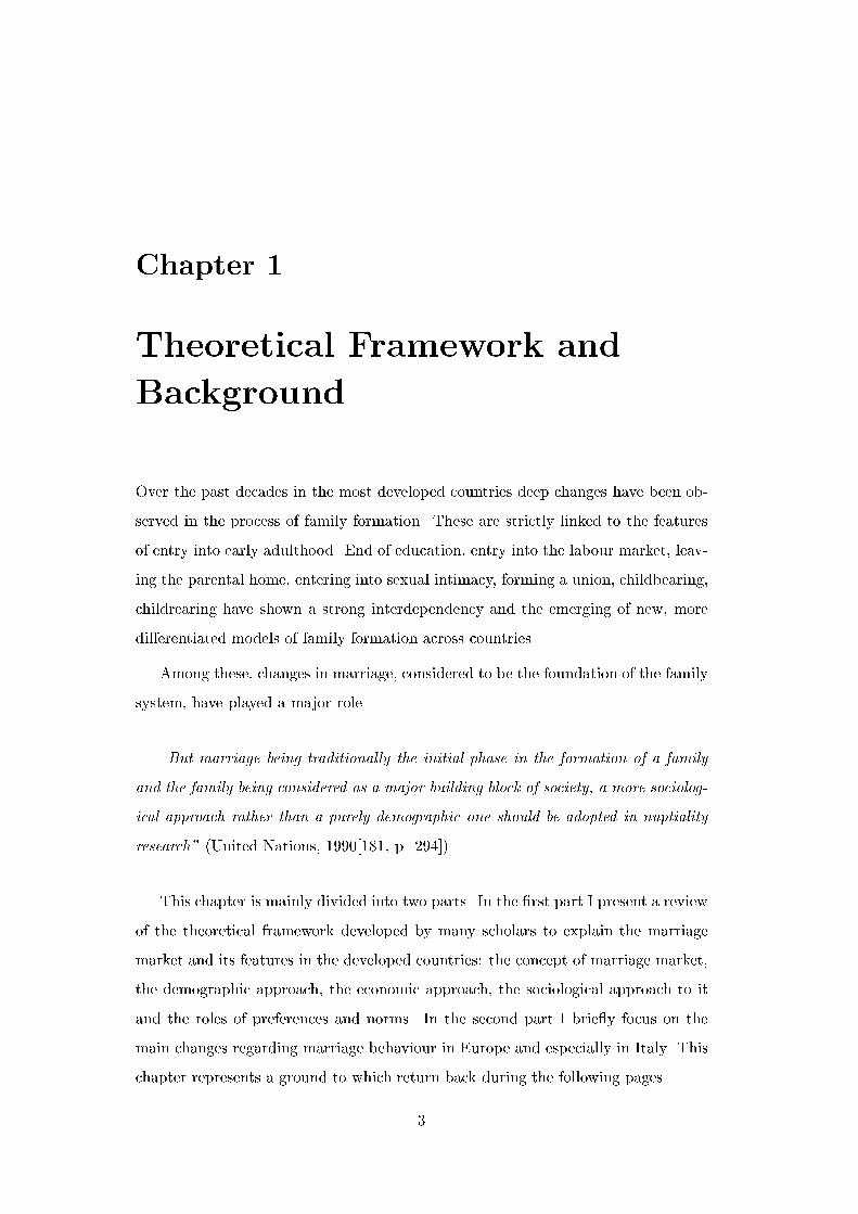
Over the past decades in the most developed countries deep changes have been ob-
served in the process of family formation. These are strictly linked to the features
of entry into early adulthood. End of education, entry into the labour market, leav-
ing the parental home, entering into sexual intimacy, forming a union, childbearing,
childrearing have shown a strong interdependency and the emerging of new, more
di�erentiated models of family formation across countries.
Among these, changes in marriage, considered to be the foundation of the family
system, have played a major role.
\But marriage being traditionally the initial phase in the formation of a family
and the family being considered as a major building block of society, a more sociolog-
ical approach rather than a purely demographic one should be adopted in nuptiality
research" (United Nations, 1990[181, p. 294]).
This chapter is mainly divided into two parts. In the �rst part I present a review
of the theoretical framework developed by many scholars to explain the marriage
market and its features in the developed countries: the concept of marriage market,
the demographic approach, the economic approach, the sociological approach to it
and the roles of preferences and norms. In the second part I brie y focus on the
main changes regarding marriage behaviour in Europe and especially in Italy. This
chapter represents a ground to which return back during the following pages.
3
4 Chapter 1. Theoretical Framework and Background
1.1 Introduction
In the popular opinion, love between two persons is able to overcome every kind of
barrier, making people blind and irrational in their actions. According to the ideal
of romantic love, in contemporary societies the selection of a partner appears to be
totally chaotic and a real matter of personal tastes.
\We grow up believing in true love, in �nding our `one and only' "
(Buss, 1994[37, p. 5]).
However, numerous studies have shown that mate selection, or assortative mat-
ing, happens in a quite systematic way1. Obviously there are clear patterns in what
can seem random: the most frequently observed pattern in assortative mating is
that according to which similars marry most often than dissimilars. In literature
this phenomenon is known as homogamy or, when it refers to marriage within a
group, endogamy, and, on the contrary, the opposite phenomenon of mating be-
tween individuals of di�erent social positions is said intermarriage, heterogamy or
esogamy.
Studies on homogamy can be roughly distinguished according to their main fo-
cus on similarities between partners regarding their social class, level of education,
employment, religion, ethnic group with the aim of measuring the level of openness
or closure of a strati�cation system of a society. A high level of homogamy, rela-
tively to the cross-sectional characteristics of a couple, means the existence of rigid
barriers between groups and of a closed strati�cation system.
For instance, researches on ethnic and racial intermarriage tries to measure the
level of integration of di�erent nationalities (Stier and Shavit, 1994[177]) while reli-
gious intermarriage is aimed at understanding the control of churches on individual's
life choice. Lastly, socio-economic homogamy is based on the idea of describing how
a strati�cation system is open, relating marriage patterns to mobility patterns2.
1\. . . but we never choose mates at random. We do not attract mates indiscriminately . . . our
mating is strategic, and our strategies are designed to solve particular problems for successful mating"
(Buss, 1994[37, p. 5])2Social inequality arises from the interplay of two mechanisms: social strati�cation and formation
of social class. The latter has its roots in the economic sphere and pursues the monopolisation and
the exploitation of scarce societal resources by creating economic and political organisations, the
former relates to interests and aims of persons and families as individual actors. Therefore inter-
and intragenerational reproduction of social inequality is the result of homogamous marriages (wife-
1.1. Introduction 5
Homogamy can therefore be considered as a mechanism to maintain the status
quo, while heterogamy an important mechanism of equalisation and interchange.
The e�ects of intermarriage are basically that it decreases the identi�cation to a
group among children as well as the negative attitudes (prejudices and stereotypes)
of individuals towards other groups3. Indeed intermarriage has been de�ned \soci-
ologically relevant" because of
\. . . its inherent dynamic. It is not just a re ection of boundaries that currently
separate groups in society, it also bears the potential of cultural and socio-economic
change" (Kalmijn, 1998[113, p. 397]).
With regard to social strati�cation system, when people belonging to high so-
cial classes marry up and those belonging to low social classes marry down, there
exist little opportunities for those with lower social status to improve their status
via marriage and higher social class people will not often cope with a descendant
mobility. On the other way round, low homogamy means the presence of a great
deal of interactions among individuals belonging to di�erent social strata, therefore
indicating a strati�cation system very open to upward and downward movements.
In such a way, homogamy, as a research topic, can be considered as a comple-
ment to the study of intergenerational social mobility, to evaluate the openness of a
strati�cation system of a society.
Many scholars today study who marries whom to understand the reproduction of
social inequality with particular attention towards the role of education (Blossfeld et
al., 1999 in press[23]; Blackwell, 1998[21]; Mare, 1991[130]). Therefore they point out
the way in which mechanisms in uencing individual and isolated marriage decisions
(at the microlevel) lead to a far-reaching reproduction of social inequality (at the
macrolevel) and, at the same time they wonder why a few people succeed in escaping
the forces of social reproduction.
husbands dimension) and of status inheritance (father-children dimension) (Haller, 1981[94]).3Evolutionary psychology focuses on early experiences, parenting, and other environmental fac-
tors to explain variability in mating strategies. (Buss, 1994[37, p. 217]).
6 Chapter 1. Theoretical Framework and Background
1.2 Theories of marriage
1.2.1 The concept of `marriage market' in the economic approach
to the demographic behaviour
Normally people do not like to think of themselves as participants in a market
when it comes to personal aspects of life such as the search for a partner. Being
compared to other individuals who compete for the same possibly scarce commodity
does not seem represent a comforting idea. This is connected to the fact that,
in contemporary western societies, the family sphere is viewed as being something
theoretically quite di�erent from the economic market, because of the strong roots
of concept such as romantic love and parental love. A market approach to marriage
has been adopted for a long time by economists (e.g. Becker, 1974 [9], 1981[10]) to
explain why people do get married or remain single, how do they live a married life,
and the frequency and causes of divorce4. Nevertheless, in the literature there is
not widespread agreement on what a marriage market is, given that each discipline
tries to focus on some of its more relevant aspects. For what we need here, the
marriage market is, broadly speaking, the place of interaction between the sexes at
the moment of the search for a partner: there, each individual neither represent a
pure object nor a pure acquirent, but he/she plays both roles at the same time, so
that a double choice, double consent must be veri�ed (Becker, 1974 [9]).
According to Becker (1981[10]), unmarried men and women can be viewed as
trading partners who decide to marry if each partner has more to gain by marrying
than by remaining single. As in all trading relationships, the gains from marriage are
based on the fact that each partner has something di�erent to o�er. In particular,
the socialisation process traditionally induces a comparative advantage of women
over men in the household because women invest mainly in human capital that
raises household e�ciency, and comparative advantage of men and women in the
labour market because men invest mainly in capital that raises market e�ciency. In
particular both men and women are viewed as participants in markets for household
labour, which in general terms includes childbearing, childrearing and other family-
related goods. Men demand wife labour and supply husband services as well as
women demand husband labour and supply wife services. By plotting aggregate
4In this work we are not going to take into account same sex couples.

1.2. Theories of marriage 7
demand and supply schedules and �nding their intersection, which represents the
equilibrium, we obtain the markets (for each sex) for household labour:
\Marriages tend to occur when at the market `wages' for female and male house-
hold labour the amount of such labour a woman wants from a husband equals the
amount of labour he wants to supply and when the amount of work this same man
wants from a wife equals the amounts of work she is willing to perform" (Grossbard-
Shechtman, 1985[91, p. 377]).
According to Becker, it is this sex speci�c specialisation of labour in our society
and the mutual dependence it produces between the sexes, that provides the major
incentive for partners to marry. Becker concludes that a rise in the earnings and
labour force participation of women reduces the gains from marriages, given that a
sexual division of labour becomes less advantageous.
1.2.2 Marriage market or marriage `markets'?
Assortative mating, mate selection and partner selection (Girard, 1981[80]) are the
most used terms to indicate the process of choice of the partner. Trying to trace the
boundaries of the place where such process develops is very di�cult and, after all
it would not be very useful. In fact, a unique \space" called the marriage market
simply does not exist as the search for a partner involves several dimensions of our
life: school, university, place of work, place of living, neighbourhood, friends, family,
relatives, cultural associations, sporting club, religious and political associations,
place of holidays, etc.
All these represent a potential marriage market: some of them may play a more
important role than others, not only because of our greater involvement in terms of
time, but also because of the higher value which we recognise or attribute to them,
and which is the result of internalised norms5. Bozon and Heran (1988[35]) distin-
guish among three main kind of places of meeting: public places, open to everybody;
reserved places, pretty heterogeneous, but for which the admission depends on the
payment of a fee or some other form of selection; private places which mainly include
family and friends.
5People develop a preference for certain spaces more than others also as a result of the segmen-
tation of the social structure: judgement categories are strongly related to interiorised categories of
perceptions, which di�er according to sex and social milieu (Bozon, 1991[32]).
8 Chapter 1. Theoretical Framework and Background
Henry (1973[97]), on the one hand, compares the relations between the sexes to
the market where the bargaining and the exchange happens and, on the other hand,
to the retort, the tool where chemical reaction between certain proportions of atoms
of di�erent elements may occur6. Nevertheless it is not enough to have just the same
number of partners of both sexes to give birth to new partnerships for everybody.
Partnership formation is a more complicated process which does not reduce itself to
passages from status of being single to married. Henry suggests a broader concept
besides that of market, as this not necessarily means binding relations. The process
of couple formation is characterised by a sequence of steps. Joining a group, a `circle
of relations', on the basis of the age of those who belongs to that group, is one of
these steps. There are multiple circles according to the geographical dispersion of a
population and each of them combine some particular ages of its individuals. Henry
(1972[96]) hypothesises that individuals choose to �t a certain circle on the basis
of their age, but then the choice of the mate inside each circle of relations is made
randomly.
According to Henry (1972[96]) there are several stages before a legally married
couple is constituted. It should be observed that the exposure to marriage is virtually
not usually discernible. The author distinguishes four stages. First, there is a
process of candidacy for marriage, when individuals are more or less conscious to
wish to get married fairly soon. Then individuals join a circle which corresponds,
at least in some respects, to the tastes of the candidate, especially insofar as age
is concerned. These two stages involve each sex independently from the other. As
a third step there is the formation of couples within these circles, and lastly, the
social recognition by marriage of the couples have been formed. The third step
takes place in the circle according to the rules that vary widely from one model to
another7. Henry recognises the fundamental role of the circle as a melting pot in
which the combining that leads to marriage takes place. Henry hypothesises that
individuals choose to �t a certain circle on the basis of their age (given that the
youngster prefer to stay with young people and the older with older), but then the
6Henry analyses the way in which two populations, composed by single individuals of each sex
(atoms), sort and give birth to a new population composed by couples (molecules). Molecules take
form when certain proportion of atoms meet (Henry, 1973[97]).7Rules can be for instance those concerning exclusions, incest, religion, height, color.
1.2. Theories of marriage 9
choice of the mate inside each circle of relations is made randomly. Moreover, the
author suggests that random celibacy may be negligible even in small population;
celibacy due to substantial variations in sex ratio by age can be spread over so many
cohorts that it becomes unnoticeably for each one of them; lastly, uctuations in
the conditional age distribution at marriage are about the same as if couple were
formed randomly in one circle, the only exception being represented by the postwar
periods.
Distance may represent a signi�cant constraint to �nd a suitable partner 8. En-
dogamy and exogamy express the possibility to marry someone who does not belong
to the same geographical group. During the twentieth century the improved com-
munication among countries and the rapidity of their di�usion has been so high to
produce a greater mobility of the people on the territory, besides a greater social
mobility, also re ected on the process of assortative mating .
The geographical proximity of partners makes the meeting and the reciprocal
choice easier. In France, a survey on assortative mating has been conducted and,
among other things, it revealed that geographical mobility is, especially in a context
of strong deruralisation of the country, a central question in understanding the
complexity of the process (Bozon and Heran, 1987[33], 1988[35], 1987[34]): to this
aim information on the residence of each partner at each signi�cant point in time of
their life cycle would also be useful. Indeed the place of birth does not re ect the
real pool of potential partners. The place of residence of the married couples, on the
other way round, gives us information on a successive moment, and therefore is not
useful to estimate the marriage market from a geographical point of view. In the
above-mentioned French study, the geographical endogamy of mates was measured
in four points in time: at their birth, during their teens, when they �rst met and
before their marriage. Evidence shows that endogamy, when measured only on the
8People used to live in small communities where the number of available mates was quite limited
and often further diminished by societal rules (due to the organisation of the society in caste or
class, for example)(Hajnal, 1965[93]). This a�ected the possibility of getting married by restricting
the circle of potential mates. To counteract this, societies reacted in di�erent ways. For example
Eastern European Jewish community had recourse to the professional `marriage brokers'; in a
system based on caste the solution mainly meant �nding a mate outside the local community, thus
promoting intermarriage with all the relevant e�ects on the social organisation and genetic structure
of the population. Moreover, marriage was used as a tool of `alliance' between families, kinship,
communities, and countries, especially by well-to-do classes and the aristocracy.
10 Chapter 1. Theoretical Framework and Background
basis of place of birth of the couple, is underestimated; a leap forward is done when
the place of residence during the adolescence is taken into account (the place of
residence during the adolescence is an indicator of the residential mobility), even
though the place were they lived before marrying is pretty close to the one where
they �rst met. This may indicate that the possibilities to choose a partner are
strongly related to the geographical constraint or that, once they make their choice,
they move less. Of course, the mobility on a territory is also a function of the social
mobility of individuals: in the same study also the socio-professional positions and
average age at �rst meeting are linked9.
But, within residential space, people do not attend the same places indiscrim-
inately: the fact that they belong to a social class may orient them towards more
frequent exchanges with some people than others. Spaces of social interaction do
have a broader meaning which goes beyond the physical environment. It is useful
then to study the assortative mating process focusing on the relations between, for
example, age di�erences and the characteristics of the place of �rst meeting between
the partners: some spaces have a very exclusive character, others a very anonymous
or familiar, closed or open one. The above-mentioned French study reveals that the
socialisation process creates a segmentation in the social universe: in fact, people
belonging to a certain social class, have more chances to meet those belonging to
the same milieu. Therefore, socialisation creates a �rst approximative selection of
the eligible; then each person evaluates the fan of alternative possibilities he/she can
a�ord on the basis of his/her own preferences.
1.2.3 The marriage squeeze
Strictly related to the concept of marriage market is that of marriage squeeze. Many
scholars studied a way to measure it (Akers, 1967[1]; Musham, 1974[139]; Schoen,
1981[162], 1982[163], 1983[164]) or to measure its causes and e�ects (Heer and
Grossbard-Shechtman, 1981[100]; Caldwell et al., 1983[38]; Goldman et al. 1984[84];
9High professionals and managers have the highest age at marriage, and the furthest pool;
unskilled working class marry younger and choose their spouse within the same common, district,
department; agricultural workers show a weak endogamy at the level of the municipalities and a
strong endogamy at the level of the district as if they were recruiting their spouses in a small area
of their country (Bozon and Heran, 1987[34]).
1.2. Theories of marriage 11
Greene and Rao, 1995[90])10. The term was introduced, for the �rst time, in 1959
to the annual meeting of the American Association for the Advancement of Science
by Glick et al. (1963[83] quoted by Glick, 1988[82]).
As many demographic, biological, social and economic factors in uence nuptial-
ity, they can sometimes cause a `squeeze' on the marriage market and on the possible
choices of people involved. Indeed this expression was introduced to refer to the ef-
fect of the baby boom in the United States: girls born during the rapid increase in
the birth rate, eventually faced a shortage of men, born few years early. Therefore
Glick et al. (1963[83]) said that the shortage of eligible men placed women in a
marriage squeeze and since then, this term has been used to describe the instability
that arises when there is a sexual imbalance in the number of marriageable persons.
The general idea is that the number of marriageable men, relative to that of
marriageable women, should be taken into account as one of the factors that in uence
decisions to get married or remain single. For example, when at an aggregate level,
more men are available for a given number of women (that is to say: there is a shift
in the aggregate demand, while aggregate supply remains unchanged) the number
of women who marry increases. Starting from the hypothesis that women prefer
marital stability more than men do, Grossbard-Shechtman (1985[91]) states that if
the wife's competitive value in the market for household labour is low and if she
has little bargaining power, she is not likely to ensure long duration marriages (thus
divorcing) or (in initial) commitment to legal marriage.
Moreover, the imbalance between the sexes, measured in terms of the sex ratios
has been linked to the spread of cohabitation and divorce (Grossbard-Shechtman,
1985[91]). From this `economic' perspective, a marriage squeeze for men which
means unfavourable conditions for them, is supposed to increase the ratio of the legal
unions to consensual unions, because some of the women involved in relations with
men will exploit the favourable market conditions to make a union legitimate, thus
decreasing the percentage of unmarried people. Therefore, under such favourable
circumstances, women are more likely to transform unions into marriages. Clearly
the converse also holds: if there is a marriage squeeze for women, which means
unfavourable conditions for them, then an increase in the ratio of nonmarital to
10For a review of the literature see also McDonald, 1995[133].
12 Chapter 1. Theoretical Framework and Background
marital unions occurs because new consensual unions will form from unmarried men
and new women, and from previously married men and new women.
Moreover, an interpretation of the spread of the feminism has suggested that,
not only the revolution in the contraceptive technology, which began in 1960, but
also the shift in the ratio of males to females at marriageable ages, which took
place in the late 1950s and early 1960s, was interconnected to the advent of the
women liberation movement (Heer and Grossbard-Shechtman, 1981[100]). In par-
ticular men during the 1950s faced a squeeze due to the decrease in the absolute
number of births at the end of the 1920 and early 1930s, and for the two-three years
usual age gap between partners; in turn, women during the 1960s coped with a
shortage of men, because of the relative rise in births at the end of the 1940 and
beginning of the 1950, and the age gap between partners. The authors suggest
that the worsening of market conditions for women, pushed them to organise and
raise women's compensation above the market level. The mechanism bargaining for
higher possible wages involves restrictions on entry into that market. According to
this interpretation, many feminists have committed themselves to singlehood (Heer
and Grossbard-Shechtman, 1981[100]). Moreover the authors suggest that the male
squeeze at the end of the 1980s will predict a period of return to a higher evaluation
of the traditional female role.
From a demographic point of view, the marriage squeeze has been basically
studied in relation to the variation in the age-sex composition due to uctuations in
fertility trends (Akers, 1967[1]; Henry, 1973[98]; Schoen, 1981[162], 1983[164]). This
sheds light on the `quantitative' features of the populations. In addition, many at-
tempts have been made to evaluate the `qualitative' characteristics of local marriage
markets in assortative mating and marital dissolution11.
However, the approach is bound by the fact that it seeks to explain only those
changes that have di�erent quantitative e�ects on the two sexes and it is not very
useful in explaining simultaneous variations (increase and/or decrease in age at
marriage) in both sexes (Oppenheimer, 1988[141]).
11There is some evidence that the increased education and labor force participation among un-
married women and the high geographic mobility rates in local areas also increase marital instability
and lower nonmarital fertility (South and Lloyd, 1992[174], 1995[176]).

1.2. Theories of marriage 13
1.2.4 Similarities and di�erences with Job-Search Theory
The matching process between partners can easily be compared to that of job search.
The basic idea regarding Job-Search Theory is that there is a distribution of potential
job o�ers for any given searcher, only a small proportion of which represents a
`perfect' match (Oppenheimer, 1988[141]). Due to the heterogeneity of labor demand
and supply, both workers and employers lack the necessary knowledge to achieve
a perfect and instantaneous matching of workers to jobs. As search has a cost,
individuals do not continue up to their perfect match, but they pursue a strategy
which consists in deciding a minimally acceptable match, in terms of wage, which is
called the `reservation' wage. Of course, the higher the reservation wage, the smaller
the acceptable proportion of jobs in the o�er distributions and the longer the time
spent searching (the probability of �nding a good match in each unit of time is low).
Therefore, the quality of match and the length of time spent searching are functions
of the reservation wage.
The matching of men and women in the marriage market is closely akin to the
matching of employers and employees in the labour market. Between the labour mar-
ket and the marriage market there are some similarities (Oppenheimer, 1988[141]).
In short: both processes are carried out under considerable uncertainty, searching
can be very costly, there exists a minimum acceptance level set by each individ-
ual, the length of time spent searching is bound up with the minimally acceptable
match and closely linked with costs and expected bene�ts. For example, the cost
of lengthy searches in the labour market presumably leads job-seekers to revise
downward the minimum wage-o�er they would regard as acceptable for employ-
ment. When jobs are scarce, unemployment increases and the reservation wage
of job-seekers declines. Analogously, lengthy searches in the marriage market may
contribute both to non marriage and to demographic mismatches between marital
partners, re ecting changes in both the relative supply and composition of eligible
men as women age (Lichter, 1990[126]).
But there still exist some di�erences between the two markets: in terms of ac-
tors, of utility function and role of the age variable. Searchers in the labour market
are simply de�ned as the unemployed who are looking for a job, while in the mar-
riage markets they are not easily de�nable. Young people start long before we can
14 Chapter 1. Theoretical Framework and Background
assume they are looking for a marital partner: moreover, people may �nd a partner
even though they are not voluntarily looking for it. This fundamental ambiguity of
marriage-search behavior indicates that the best strategy is to focus on measuring
what conditions foster or impede successful matches.
As regard the utility function, in the labor market it is represented by the in-
come people expect to gain, while in the marriage market it does not have a directly
measurable de�nition, because it is a more complex function: it involves not only
socioeconomic status, but also long-run intimacy, emotional support, companion-
ship, children, sex, etc. In brief, not only socio-economic characteristics have to be
accounted. It is probably not highly meaningful to try to operationalise marriage
utility as we do with the reservation wage.
But probably the most important di�erence which emerges between the two
markets is the one regarding the role of age: in fact in the marriage market it
assumes a very important role related to its meaning.
First of all, the shape of the distribution of potential partners does change dra-
matically with age and, with it, the e�ciency of the search process (given that
marriage progressively thins out the eligibles - Goldman et al., 1984[84]; Diekmann,
1990[67]; Raley, 1996[148]).
Second, a dynamic development in the characteristics of individuals occurs with
age. This might represent a reason for the greater instability observed for early
marriages as future characteristics are unknown at young ages. Exogenous factors
may a�ect the predictability of the future characteristics of the partner. Postmarital
socialisation process has been invoked as a factor that may reduce unpredictability.
Third, the decision to accept a particular match does close o� to other oppor-
tunities in future. There is an opportunity cost which is higher at younger ages.
Conversely, later marriages, even though not as desirable as those refused earlier,
may be accepted because of a shift to lower acceptance level. The risk of a marriage
less desirable than the one refused earlier is higher for women, given that they more
often marry older men. The supply of potential males decreases with age for women,
while the supply of women increases with age for men (Goldman et al., 1984[84]).
The result of the search will therefore depend not only on the number of suitable
partners, but also on the reliability of information about important characteristics
1.2. Theories of marriage 15
of both the searcher and potential partners. Both these two elements change with
age: the availability of potential partners decreases with age, while the reliability of
information increases with age. Thus, the constant interaction between the avail-
ability of partners and the reliability of information determines the variability of the
timing process (Oppenheimer, 1988[141]).
1.2.5 Elements of uncertainty
Uncertainty is due to the lack of knowledge regarding either potentially alternative
partners or to changes of the current partner's attributes. Some of the traits which
characterise a partner may be unknown at the moment of the choice or they may
successively change with age by acquiring new adult and unexpected roles. Accord-
ing to Barbagli, (1990[6]) many sociologists and economists agree that people who
marry very young have high probability to divorce because they devote a few amount
of time to the choice of their partner, therefore acquiring an insu�cient amount of
information on the marriage market. Making long-term matches, implies also
\estimating the nature of the future characteristics on the basis of the incomplete
information currently available" (Oppenheimer, 1988[141, p. 571]).
Sometimes a period of courtship or cohabitation may, to a certain degree, be
helpful in reducing uncertainty, as well as the postmarital socialisation can com-
pensate for part of the imperfect predictions made during the selection process.
Moreover, those who have been married and who have had children in a previous
marriage, are a�ected by a greater uncertainty due to their lower attractiveness.
Of course a reduction of the uncertainty can be achieved by focusing on the cur-
rent characteristics of the partner, which are, somehow explicative of his/her future
resources. Education, occupation, ethnic group, family background can reduce the
degree of uncertainty and can help in the �ltering process of spouse selection (Goode,
1964[88]). Among all these various badges that characterise individuals, the most
important role is assigned to work (Oppenheimer, 1988[141], Kalmijn, 1994[112]):
it is expression of the value, lifestyle and prestige of a person.
As we said above (see 1.2.4) the timing of marriage depends on the interaction
between availability of potential partners and on reliability of information. Early
marriages may therefore be a�ected by a greater instability, as their success depends
16 Chapter 1. Theoretical Framework and Background
on how well the prediction about the future characteristics of the partners and their
future lives together will be like. Obviously also exogenous factors play a very
important role in a�ecting future predictions. In any case postmarital socialisation
acts as a compensation process.
Then, both the available number of `suitable' partners and the reliable informa-
tion about their characteristics a�ect the success of the search. These aspects of
marriage market are assessed in terms of quantity and quality of its actors (Scott
and Lloyd, 1992[174], 1995[176]; Raley, 1996[148]). As the availability of potential
partners decreases with age, the `optimal time for marriage', if de�ned on the basis
of the greatest number of unmarried persons, is supposed to be at relatively young
ages, wheras, if de�ned on the basis of the highest information available on assorta-
tive mating attributes, is probably at relatively old ages (Oppenheimer, 1988[141];
Danziger and Neuman, 1999[59]). Moreover a certain degree of free will of the indi-
viduals should be allowed, even if they are supposed to act rationally (Blossfeld and
Timm, 1999[23]).
1.2.6 Marriage-Timing Theory
Age patterns
The well-known age distribution of �rst marriages by sex consistently reveals the
existence of a nonmonotonic, bell-shaped pattern observed for di�erent countries,
periods, and socioeconomics groups. The �rst marriage age distribution corresponds
to a left-skewed unimodal frequency distribution, whose regularity has been often
referred to the existence of a law governing the marital process. In particular three
type of models have been proposed. For the `latent state model' the age at mar-
riage is the result of two components: a random variable referred to the duration
of the latent state `not in search of a mate' and duration of the latent state `in
search of a mate'. For instance Coale and McNeil (1972[51]) assumes that the wait-
ing time until entering the search state is normally distributed and that the search
time prior to transition to marriage is the sum of exponentially distributed waiting
times. In particular, once in search of a mate, there is a waiting time (exponen-
tially distributed) before the �rst meeting, then a waiting time before the dating
(exponentially distributed) and, lastly, a waiting time before marrying.

1.2. Theories of marriage 17
A second model is that based on the `unobserved heterogeneity model'. In the
rational search process under imperfect information, for each individual there is a
linear increase with age in the transition rate to marriage, but as the rate varies in
the population, we observe, in the overall population a nonmonotonic aggregated
pattern.
The third group of model is the `di�usion model', introduced by Hernes in
1972([99]). This model assumes the existence of a kind of contagion process among
individuals at their marriageable ages. Those already married of the same cohort
exert a a social pressure to marry. For an applications to the Italian case of the
three models see Billari (2000[18]).
Age di�erences among partners
Understanding the reasons of the timing of marriage has been a central aim of
researchers of di�erent disciplines. For example, economists mainly analysed the
in uence of the entry into the labour market on the acquisition of adult economic
role and on the age at marriage of both sexes (Becker, 1974[9], 1981[10]; Danziger
and Neuman, 1999[59]).
Sociologists' studies on marriage timing, highlight gender and social di�erences
in close connection with strati�cation system and chances of social mobility (Goode,
1964[88]; Haller, 1981[94]; Oppenheimer, 1988[141]).
Demographers mainly point out changes in marriage timing as a result of struc-
tural variation of the population size due to variations in the natality rates across
birth cohorts and in di�erential mortality between sexes (Henry, 1975[98]; Festy,
1971[72]; Bartiaux, 1994[8]).
Trends and di�erentials in marriage timing result from variations in the de-
grees of di�culty people encounter in mating assortatively. A great deal of studies
have developed theoretical frameworks where the assortative mating is linked to
transition to the economic roles both in traditional and in contemporary societies
(Oppenheimer, 1988[141]; Danziger and Neuman, 1999[59]).
Many economists studied the age di�erences between partners. The timing of
marriage has been linked to the problem of the searching process. According to
Becker's neoclassic Theory of Marriage (1974[9], 1981[10]), household commodities

18 Chapter 1. Theoretical Framework and Background
cannot be purchased in the market and are most e�ciently produced by combining
the time inputs of two spouses. Bene�ts from marriage increase with the extent to
which spouses' time jointly produces household commodities. Furthermore, if both
spouses are working and the husband's wage rate exceeds the wife's wage rate, an
increase in the husband's wage rate or a decrease in the wife's wage rate will increase
the bene�ts from marriage since the husband will specialise more in the market work
and the wife more in the household production. In the absence of uncertainty and
costs of marriage, each individual either marries the most desirable individual, or
stays single, if the net gain frommarrying any potential spouse is negative. Therefore
the ensuing equilibrium in the marriage market maximises the aggregate gain from
all marriages. In case of uncertainty about the characteristics of potential spouses,
marriage is costly: the individual spends time and other resources searching for the
best attainable match. Therefore the age at marriage depends both on the expected
gains from marriage and on the costs of �nding a suitable spouse.
In 1977, Keeley[117] (quoted by Danziger and Neuman, 1999[59]) combines
Becker's theory and search theory de�ning the age at marriage as the sum of the in-
dividual's starting age at search and the length of the search period. Larger expected
gains from marriage induce people to marry younger. In particular Keeley states
that if wage rates are higher for men than for women, a man's optimal marriage age
decreases with his wage rate, while a woman's optimal marriage age increases with
her wage rate, because her direct costs of search are greater and her expected gains
from marriage are smaller. That is to say, for men there is an anticipation of the
marital behaviour, while for the women there is a postponement.
In traditional societies, where only males earn an income, age at marriage is
strictly linked to the problem of information (`revelation problem'): young men,
who believe they are likely to become economically successful, postpone marriage in
order to prove their ability and increase their appeal to more desirable women, while
young men who do not think they are likely to command high earnings later in life,
choose to marry young (Bergstrom and Bagnoli, 1993[13, p. 181]). In traditional
societies, women do not earn any income and their value in the marriage market
depends only on their ability in household production, therefore to their potential
partners the postponement of marriage does not help in revealing much additional
1.2. Theories of marriage 19
information about them. Hence, in this model all women marry young: the more
desirable women marry with the older successful men and the less desirable women
marry the young men who are less likely to command high earnings. In contrast
to Becker and Keeley, Bergstrom and Bagnoli obtain that a man's optimal age at
marriage increases with is wage rate. The di�erence between the two theories is
due to the fact that the latter is mainly referred to traditional societies where the
earning power of men is particularly important.
Because of reproductive constraints, age di�erences at marriage between men
and women are supposed to re ect sex di�erences in human reproductive strate-
gies: the sociobiological explanation (Otta et al., 1999[142]) of the age di�erence
at marriage is based on the assumption of the sexual bimaturism of our species,
according to which women mature 2 or 3 years earlier than men. Also from the
evolutionary (psychological and anthropological) point of view all mating behaviour
entails changes over time. For instance, a woman's desirability as a mate is strongly
determined by signals of her reproductivity, whose value generally diminishes as she
gets older (Buss, 1994[37])12. While women's desirability as mates declines steeply
with age, the same does not apply to men's. Men's value in supplying resources,
indicated by features such as income and social status, shows a markedly di�erent
distribution according to age than women's reproductive value. To this regard, there
are two important di�erences between the sexes: men's resources and social status
typically peak much later in life than women's reproductive value, and men di�er
more markedly from one another in the resources and social status they accrue13.
Given the di�culties in measuring social status, evidence shows that in no known
culture do teenage boys enjoy the highest status. In contemporary western societies
income tends to be quite low among men in their teens and early twenties, while it
12The downturn of a woman's desirability is shown in some societies where women are literally
purchased by men in return for a bride price. The �nal price, set by bride's father after considering
all competing o�ers and demanding a higher price, depends essentially on the perceived quality of
the bride. The higher the reproductive value of the bride, the greater the bride price. Moreover
several other factors lower a woman's value to a prospective husband and hence lower her price as
a potential bride: a physical handicap, pregnancy, the existence of a child from previous man, etc.
(Buss, 1994[37]; Bhat and Halli, 1999[17]).13In ancestral gatherer-hunter societies, men did not vary in the amount of their resources but
they did vary with regard to their social status. Contemporary societies show di�erences, bigger
than in ancestor societies, in the amount of resources distributed among their individuals and
smaller than in ancestor societies in status di�erences among them (Buss, 1994[37]).

20 Chapter 1. Theoretical Framework and Background
rises thereafter.
Therefore, if we consider men and women at the same age, they di�er on average
in their value as mates. If the central component of a woman's desirability is her
reproductive value and that of a man's is his resource capacity, men and women of
the same age are not typically comparable in their desirability. Moreover, because
of a greater variability among men, age per se is a less in uencing factor in mating
for men.
Marriage squeeze as women age, from a psychological point of view, is in large
measure an outcome of the sexual psychology of men and women.
\At the heart of the squeeze is the sharp decline in female reproductive value with
age, which caused selection to favor ancestral men who preferred younger women
as mates and to favor ancestral women who preferred older men with resources as
mates"(Buss, 1994[37, p. 203]).
Age di�erences between spouses can also be a sensitive indicator in the analysis
of the general context of gender di�erences and the recent changes in nonmarital
unions. For example, evidence shows, that in the cases of unions of single cohabi-
tants, age di�erences between partners are small, while in the case of �rst marriages
without prior cohabitation age di�erences are higher, especially when the woman
is very young or with very low education. Therefore, it emerges that women with
higher occupational precariousness, because younger and less educated, prefer to
be `dominated' by the age of their man; on the contrary young men are largely
indi�erent to the age of their mate (Bozon, 1990a[30], 1990b[31]).
Attempts have been made to test whether age heterogamy may also a�ect the
whole quality of the marriage, but age heterogamy seems to be strictly related to
socioeconomic and ethnic groups. In the United States, age heterogamous marriages
have been substituted by a great proportion of age homogamous marriages, and this
has been interpreted as an e�ect of the equalisation process (Vera et al., 1985[186];
Atkinson and Glass, 1985[5]).
Gender speci�c and origin speci�c nuptiality models
Acquiring adult economic roles is a crucial step in the transition into adulthood
especially as regard timing. For those who want to get married, the entry into

1.2. Theories of marriage 21
the labour market may signify a step forward marriage, and, moreover, this pro-
cess structures life in many ways, not only for the workers themselves, but also for
those close to them. Given the strong role of work in the timing of marriage, it is
interesting to investigate whether it plays a di�erential role on the genders. Oppen-
heimer, 1988[141] analyses the system of functioning of the marriage market both
in a traditional society and in a modern one.
Parsons, as well as Becker, emphasises the importance of gender segregation of
roles for the stability of the family and even for the society itself (1949[144]). From
his point of view, gender segregation of roles, which destines women to be mothers
and housewives, is functional to the harmony of the couple and of the family as a
whole, as it prevents competition between partners.
Also Becker argued that the more di�erent the trade to bargain between women
and men, the more the advantage from it: thus women highly specialised in house-
hold production and men highly specialised in work production, maximise their gain
from marriage. Moreover, positive assortative mating for complementary traits (ed-
ucation, intelligence, attractiveness) and negative assortative mating for substitutes
(income) occur: men with high earnings potential marry women with low earnings
but which are superior with respect to other characteristics. According to the New
Home Economic, the labor force participation of women has weakened the gain from
marriage and has become the main reason for the increasing divorce rates, as the
bene�t for strong division of roles has greatly diminished (Becker, 1981[10]).
Let us imagine a traditional society where only men work and women are, there-
fore, strictly dependent, in their socioeconomic status, on the status of their hus-
bands. As a young man does not possess a clearly identi�able position, especially
if he aims at socioeconomic upward mobility, his future is quite uncertain and this
will a�ect his chances to marry young. The high cost of search and uncertainty may
force him to either decide to lower his minimum acceptance level, thus marrying
young, or to improve his economic position, thus marrying later14. Nevertheless,
sometimes the postponement of marriage, due to low income earnings of the male,
can be contrasted with her earning capacity when the wife works during the early
14Premarital sex, in contemporary societies, reduces the high cost of postponed marriage, allowing
a delay in marriage timing (Oppenheimer, 1988[141]).
22 Chapter 1. Theoretical Framework and Background
years of marriage: therefore, if she collaborates in the labour market and if they
succeed in controlling fertility for a while, age at marriage can be lower than usual.
In such a traditional society, women's traits are already de�ned at young ages and
their reproductive capacity declines from their middle twenties. For Becker, women
satisfy their advantage as soon as they marry and, as regard their future, women
have much lower uncertainty than men do. Therefore, because the supply of avail-
able men to them is decreasing with age, women normally have a faster transition
to marriage than men. This also implies di�erent ages among spouses, especially
when women are very young (Bozon, 1990[31]). To prevent daughters from mar-
rying, families used to increase their advantages and attractiveness by the dowry
system: it also functions to strongly contrast the declining supply of men as girls
get older (Goode, 1964[88]; Oppenheimer, 1988[141]; Buss, 1995[37]; Bhat and Halli,
1999[17]).
Let us now imagine that women work for a longer period of time, not just before
having their �rst child, which is the case for most of the developed countries. Several
hypotheses have been developed to demonstrate that increasing female labour force
participation has produced, by a greater economic independence, delay in marriage,
rise in divorce, strong marital instability and eventually decline in fertility (Becker,
1974[9], 1981[10, chap.10]; Davis, 1985[60]). In the United States, the change in
the rates of marriage are found to be linked to the reduced willingness of women to
marry and to their increased ability to support themselves outside marriage, instead
of to some constraints on the marriage market which, anyway, operates in the same
direction for both sexes (Goldscheider andWaite, 1986[85]). Nevertheless, job-search
theory may highlight the role played by other factors, as well. For example, schooling
has increased its importance as a tool to improve the chances for a good job. As a
consequence, early marriages may represent an obstacle to this aim. Another factor
which may bring about a delay in marriage for working women is linked to the greater
e�ort required by the adaptive socialisation process. Although the mechanism of
the assortative mate selection has remained unchanged, the socialisation requires a
more intensive commitment: if both partners are workers, they have to pool their
energies and to cooperate in a better way. Thus, postmarital adaptation may be
no longer su�cient as a compensation mechanism. A period of cohabitation may
1.2. Theories of marriage 23
represent an alternative way of living, pooling together the advantages of marital
relations, but, at the same time, still allowing a certain degree of independence
and reciprocal knowledge. In this sense premarital cohabitation may represent a
`prelude' to marriage (Villeneuve-Gokalp, 1994[187])15. Lastly, earning money for a
woman may increase her attractiveness, even at increasing ages, and may enlarge
her marriage market (also thanks to the directly enlarged labour market in which
she is involved). According to Oppenheimer[141] the greater instability of marital
unions may well be linked to the recent and fast changes in contemporary societies.
Exogenous factors
Several changes in marriage timing patterns depend, both cross-sectionally and lon-
gitudinally, on exogenous factors such as, for example, changes occurring in the
labour market. The demand for highly specialised professionals, requires a length-
ening of the period of study and, in some cases, also higher geographical mobility
during the training period, and therefore a postponement of the timing of marriage
(Oppenheimer, 1988[141]; Mare, 1991[130]). Moreover, di�erences in the timing of
marriage among working men will depend on their involvement in the type of career
they want to reach (white collars versus blue collars).
Oppenheimer (1988[141]) argues that young men's income position is an ex-
tremely important factor a�ecting the timing of marriage of both men and women.
The increase in the age at marriage can therefore be explained by the weak posi-
tion on the labour market that young men occupy, linked to their uncertainty: even
promising men may have a low entrance income16. In addition, periods of economic
crisis or war directly a�ect marriage conditions. Therefore, at least in the American
society, the author observes that most of the changes in marriage timing are still
15However, it should be observed that the relation between premarital cohabitation and marriage
is not clear, as for marital dissolution seems to be higher for those who previously cohabited (Waite,
1995[189]).16Oppenheimer insists on the point that it is the deterioration in young men's labour market
position the more likely explanation of the changes in male marriage timing and perhaps of female as
well. According to Easterlin, the recent sharp decline in the relative economic position of young men
can be mainly attributed to the entry into the labour market of the baby-boom cohort. Therefore,
the situation should reverse once the baby-bust cohort arrive. Still Oppenheimer observes that
the cause of the delay in the transition to a stable work career is due to the shift towards more
professionalised occupational structure characterised by relatively steep age-earnings pro�les and
this situation would not improve once the baby bust cohort will arrive.

24 Chapter 1. Theoretical Framework and Background
the consequence of the changes in the young men's economic position, instead of the
increased economic independence of women.
1.2.7 Homogamy through preferences, expectations, orientations
and norms
Marital unions are characterised by a complex web of long-term trust and reciprocity
that appears to be unparalleled in other species (Buss, 1994[37, p. 221]). In this
sense, the cooperation between sexes reaches a pinnacle among humans. From an
evolutionary point of view two `sexual strategies' exist17: as adaptations are evolved
solutions to the problems posed by survivals and reproduction, correspondingly,
sexual strategies are adaptive solutions to mating problems.
From the point of view of evolutionary psychology (Buss, 1994[37]), ful�lling
each other's evolved desires is the key to harmony between a man and a woman.
Therefore, a woman's happiness increases when the man brings more economic re-
sources to the union and shows kindness, a�ection and commitment, while, a man's
happiness increases when the woman is more physically attractive than he is, and
when she shows kindness, a�ection, and commitment. From this perspective, those
who ful�ll each other's desires have a more successful relationship18.
Assortative mating has already been de�ned as a quite complex phenomenon in
which many choice mechanisms interact. At an aggregate level, marriage patterns
arise from the interplay of three social factors: preferences at the individual level,
in uence of group level factors and structural constraints (Kalmijn, 1998[113]).
As we said with respect to that concept, on a marriage market each individual
evaluates his/her set of potential spouses, on the basis of their resources and in the
perspective of increasing `familiar', not individual's, goods. To this aim di�erent
kinds of resources can be distinguished and the main ones are the following two:
1) Socioeconomic resources that produce economic well being and status: from
17The term `strategy' is used as a metaphor: sexual strategies do not require conscious planning
or awareness (Buss, 1994[37, p. 6]).18According to Buss (1994[37]), typical of humankind is that two unrelated individuals can bring
all of their individual resources into a lifelong alliance characterised by love. Some of these resources
tend to be linked to a person's sex, such as a female's reproductive viability or the male's provisioning
capacity. But mating resources typically transcend these reproductive essentials to include such
capacities as protection from danger, deterrence of enemies, formation of alliances, tutoring of
children, loyalty in times of absence, and nurturance in times of sickness.
1.2. Theories of marriage 25
the competition for them there is a strong selection among the most attractive
candidates and the least attractive ones have to rely on one another, and this
phenomenon produces homogamy. The competition for these resources, which
is aimed to marry someone of high status, is strictly dependent on the role
of women in a society. In a traditional society, for example, the exchange
happens between man prestige (in terms of paid labour) and woman qualities
(household labour). In contemporary societies this has changed as women in
the labour market have increased their attractiveness to men. In fact, wife's
human capital is seen as a way to help husband's access to higher career.
2) Cultural resources in terms of values, worldview, knowledge: such kind of
similarities have been studied by psychologists. People prefer to marry some-
one with cultural similarity, because this makes easier taking decisions about
their future plans, daily life, children's education. Cultural similarity has been
recognised as being successful in establishing long-term relationship, because
it ensures common basis of conversation, provides con�rmation on one's norms
and values and reduces the friction within marriage that may arise from dis-
similarities.
Some authors think that social characteristics are correlated with socioeconomic
and cultural resources and that homogamy and endogamy are by-products of the
individual preferences for resources in a partner. For instance, although related to
income and ascribed status, educational homogamy can also be the result of com-
mon taste, values and lifestyles developed by those who have been longer involved
in the educational system19. For others, social characteristics such as education,
occupation, race, ethnicity may be used to show individual features and to enter in
a kind of spouse selection process: people �rst select the network of friends and ac-
quaintances with similar characteristics and then choose their partners among them
homogamously (Goode, 1964[88]; Henry, 1973[97]).
The in uence of group level factors can be understood if we focus on people
who are not directly involved in marriage. Kalmijn (1998[113]) refers to them as
`third parties': they develop incentives or sanctions to avoid new generations from
19In a recent study on recently married couples in the U.S. emerged that assortative mating by
cultural status is more relevant than assortative mating by economic status (Kalmijn, 1994[112]).
26 Chapter 1. Theoretical Framework and Background
marrying exogamously. Each individual develops, at a di�erent level, the so-called
`sense of peoplehood' linked to norms that are accepted by his/her society. Group
identi�cation is normally due to the socialisation process and to the network. Ed-
ucation has an important role in this context as it weakens the identi�cation in a
group, therefore increasing intermarriage (Kalmijn, 1988[113]).
At the same time, even for those who do not interiorise norms of endogamy,
there may be a force that presses them to certain behaviour. Institutions may use
direct or indirect sanctions to enforce their norms. For instance, the family, the
church and the state may adopt groups' sanctions against exogamous marriages.
Sanctions and norms developed as a form of protection and consolidation against
the external forces20. Therefore, in this context, the family may neglect its support
and approval, the church can denounce interfaith marriages, and the state may
segregate racial intermarriages.
Lastly, not only individual and group-level factors, but also structural arrange-
ments govern endogamy and homogamy. There is more than one structure arrange-
ment: demographic composition of a population, regional distribution of groups,
functional of settings (such school, workplace, and neighbourhood) can represent
some of the constraints. Basically they act in terms of quantity and quality of the
number of eligibles in the marriage market. First of all, the e�ect of group size
implies that endogamy is negatively related to the degree of heterogeneity of a pop-
ulation (Kalmijn, 1998[113, p. 402]). Moreover, the distribution of a population on
a geographical area is crucial as isolation may contribute to high endogamy.
The characteristics of local marriage markets, such as schools, workplaces, and
neighbourhoods, are extremely important in explaining marriage patterns. The
school, for instance, is the most e�cient market because it is homogeneous with
respect to age and heterogeneous with respect to sex. The workplace is considered
less e�cient even though the increasing participation of women in labour market
may change its role (South and Lloyd, 1995[176]).
A central message of human sexual strategies is that mating behaviour is enor-
20`Di�erences in mean age at �rst marriage exist among rural women as well as among women
with the same level of education in di�erent countries. Because standard socio-economic indicators
are not su�cient to account for the observed behaviour, more attention needs to be devoted to
the socio-cultural factors involved, in particular to the marriage norms prevailing among these
population subgroups' (United Nations, 1990[181, p. 294]).
1.3. Recent studies in Europe and Italy (and US) 27
mously exible and sensitive to social context. Di�erences between the genders
appear to be universal features of our evolved selves. Cultural variation represents
one of the most fascinating and mysterious aspects of human diversity. Therefore
men and women follow their preferences and expectations in terms of assortative
mating under the constraints expressed by the social and cultural environment in
which they live. The more the context is open to the external interchange, the higher
the presence of intermarriage.
1.3 Recent studies in Europe and Italy (and US)
In 1990 the United Nations[181] stated about the role of the marriage market:
\. . .Despite considerable insights achieved by available marriage market studies,
there are still di�culties in assessing quantitatively the e�ect of the marriage market
and especially in distinguishing its interactions with social factors. In addition, social
adaptability to market imbalances needs to be further studied." (United Nations,
1990[181, p. 294])
Nowadays, researchers still agree with the importance of studying marriage, de-
spite of recent and increasing changes in the model of family formation in developed
countries (United Nations, 1990[181]; Leridon, 1991[120] ; Roussel, 1992[154]; De
Sandre et al., 1999[65])21.
From a theoretical point of view, either at a microlevel and at a macrolevel ex-
planation, the decline in marriage, the increase in divorce, the rise in cohabitation
and in the birth out-of-wedlock have been linked to the decline in the advantages
of marriage. Long term socioeconomic and cultural trends have (slowly) modi�ed
individual preferences, constraints, opportunities and, at the same time, the mean-
ing of marriage has changed. As the trends towards decline and postponement of
marriage, emergence of cohabitation and increase in marital instability have been
common to most of western countries, theories have been developed to shed light,
at a macrolevel, on these almost universal demographic patterns. A summary of the
changes in the marriage related demographic behaviour observed in the European
21Evidence from a recent survey in Italy shows the existence among Italian women and men, also
and above all those belonging to young generations, of a strong attachment towards marriage: . . . it
still appears as a fundamental value and this places Italy in a quite singular situation with respect
to the other European countries, especially the Northern ones. (De Sandre et al., 1997[64])
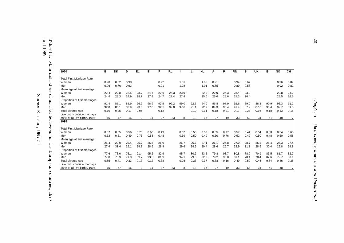
28
Chapter
1.Theoretica
lFramew
ork
andBackground
1970 B DK D EL E F IRL I L NL A P FIN S UK IS NO CH
Total First Marriage RateWomen 0.98 0.82 0.98 0.92 1.01 1.06 0.91 0.94 0.62 0.96 0.87Men 0.96 0.76 0.92 0.91 1.02 1.01 0.85 0.89 0.58 0.92 0.82Mean age at first marriageWomen 22.4 22.8 22.5 23.7 24.7 22.6 25.3 23.9 22.9 22.9 24.3 23.4 23.9 22.8 24.2Men 24.4 25.3 24.9 28.7 27.4 24.7 27.4 27.4 25.0 25.6 26.6 25.3 26.4 25.5 26.5Proportion of first marriagesWomen 92.4 86.1 85.9 96.2 98.9 92.5 99.2 99.0 92.3 94.0 86.8 97.9 92.6 89.0 88.3 90.9 93.3 91.2Men 92.0 86.1 83.9 93.6 97.6 92.1 99.0 97.6 91.1 92.7 84.3 96.4 91.4 87.9 87.6 90.4 92.7 89.0Total divorce rate 0.10 0.25 0.17 0.05 0.12 0.10 0.11 0.18 0.01 0.17 0.23 0.16 0.18 0.13 0.15Live births outside marriage
as % of all live births, 1995 15 47 16 3 11 37 23 8 13 16 27 19 33 53 34 61 48 71995
Total First Marriage RateWomen 0.57 0.65 0.56 0.75 0.60 0.49 0.62 0.56 0.53 0.55 0.77 0.57 0.44 0.54 0.50 0.54 0.63Men 0.52 0.61 0.49 0.73 0.58 0.48 0.59 0.50 0.49 0.50 0.76 0.52 0.42 0.50 0.48 0.50 0.58Mean age at first marriageWomen 25.4 29.0 26.4 25.7 26.8 26.9 26.7 26.6 27.1 26.1 24.8 27.0 28.7 26.3 28.4 27.3 27.4Men 27.4 31.4 29.1 29.8 28.9 28.9 29.6 28.9 29.4 28.6 26.7 28.9 31.1 28.5 30.4 29.8 29.8Proportion of first marriagesWomen 77.6 73.0 76.1 91.4 95.2 82.9 95.7 80.2 83.5 79.8 93.7 80.8 78.9 70.9 83.5 81.7 82.7Men 77.0 73.3 77.0 89.7 93.5 81.9 94.1 79.6 82.0 79.2 90.8 81.1 78.4 70.4 82.6 79.7 80.1Total divorce rate 0.55 0.41 0.33 0.17 0.12 0.38 0.08 0.33 0.37 0.38 0.16 0.49 0.52 0.45 0.34 0.46 0.38Live births outside marriage
as % of all live births, 1995 15 47 16 3 11 37 23 8 13 16 27 19 33 53 34 61 48 7
Table
1.1:Main
indica
tors
ofmarita
lbehaviourin
theEuropeancountries,
1970
and1995
Source:
Eurosta
t,1997[71]

1.3. Recent studies in Europe and Italy (and US) 29
countries between 1970 and 1995 is reported in table 1.1. The decreasing attrac-
tiveness of marriage, observed as a reduction of nuptiality rates and an increase of
divorce rates, has been explained by the complexity of the structure of the underlying
social, economic and cultural changes. Although it is di�cult to �nd a set of most
in uencing factors, it is usually recognised that rapid changes in fertility, marriage,
divorce and cohabitation appear because of a mixture of socioeconomic and cultural
factors (Van de Kaa, 1987[184], Lesthaeghe and Surkyn, 1988[124]): urbanisation,
industrialisation, emancipation, the rise of the welfare state, individualisation, sec-
ularisation. This complex structure of factors has determined shifts in individual
preferences (towards more individuality, freedom, independence), in constraints (to-
wards less normative constraints and less a�rmation to institutional regulations of
the state, the church or the family) and opportunities (women's economic indepen-
dence through labour market participation and individualisation of social security).
Structure, culture and technology are according to Van de Kaa, three basic interre-
lated social dimensions among which one can search for an explanatory framework
of the deep demographic changes occurred in the past decades: the complex set of
transformation which they involved are known as Second Demographic Transition.
Secularisation and individualisation are long-term cultural changes that have mod-
i�ed individual preferences in terms of marriage and divorce. `Silent Revolution' is
the most used term to refer to changes occurred in the cultural dimension. During
the seventies, when marriage was perceived as `bourgeois', the growing importance
of individual's self-ful�lment and the weakening of the normative guidelines, have led
to the decline of marriage and the rise of divorce. This shift in individual preferences
occurred together with a shift in individual opportunities for the free choice.
According to Van de Kaa[184], structural changes are: modernisation, increase
in the standard of living and social security bene�ts, functional di�erentiation,
widespread of increasing education, women's increasing earning of power. Espe-
cially the last factor has been addressed by the economic theories (Becker 1974[9],
1981[10]) as the major factor in reducing the expected gain of marriage22. The in-
22Historically through marriage women gained economic support from the husband whereas men
gained support regarding domestic services from the wife. The rise in the earning power of women,
resulting from increasing education and labour force participation has disturbed this traditional
gender based division of labour.
30 Chapter 1. Theoretical Framework and Background
creasing earning power of women has also increased the opportunity costs of children,
because childbearing often coincides with a woman's exit from paid employment.
Researchers agree in attributing the main cause of the risk of divorce to the
changes observed in marriage as regard to its value, its function, its advantage.
Changes in divorce can only be properly understood by related changes in marriage.
Macro sociological theories highlight the loss of societal functions of marriage as the
main reason of its decline (Espenshade, 1985[70]). Others refer to the declining pref-
erence or `taste' for marriage (Bumpass, 1990[36]). According to Roussel (1989[153]),
the shift from material to immaterial advantages of marriage is an underlying cause
for rising divorce trends23.
The last very important factor which facilitated the move away from marriage is
technological change: for example the availability of good contraception, known as
`Second contraceptive revolution', allowed the increase in the age at �rst marriage
because it enabled couples to avoid the fear of pregnancy. This revolution was
also facilitated by the spread of more information both by transport system and by
communication means.
The lengthening of youth, which characterises the period between adolescence
and adulthood autonomy, is a general phenomenon in Europe opposed to the tra-
ditional model, according to which the entry into adulthood is characterised by a
strong synchronism of steps along two main axes: on the �rst axis, the educational-
occupational one, we register end of studies and entry into the labour market, and
on the second axis, the familiar-conjugal one, we observe exit from family of origin
and marriage. Despite a great number of di�erences in calendars within genders and
social origins, synchronism is intended to be due to the traditional sequence among
phases: the end of study is normally followed by �nding of the �rst job which pro-
vokes, after a while, the exit from parental family and then the marriage. In the
traditional model, youth has a very marginal role: it is a privilege basically of the
bourgeoisie and of the males (Galland, 1993[73]). Nowadays in Europe the tradi-
23Remarriage plays a very important role in the debate regarding marriage as an institution.
Kalmijn and de Graaf (2000[114]) observe that if remarriage rates are high, it is not very sensible
to regard divorce as a sign that the institution of marriage is fading. The combination of frequent
divorce and frequent remarriage points to other factors that may cause marital instability and
suggest that a model of sequential marital monogamy �ts the present situation better.if a low rate
of remarriage is compensated by a high rate of cohabitation, the thesis of a weakening marriage
institution is still a potentially valid interpretation of demographic trends.

1.3. Recent studies in Europe and Italy (and US) 31
tional model has been substituted by a new series of intermediate situations between
adolescence and adult autonomy which shows a trend somewhat cross-national. In a
very general way, four typologies of models regarding the adulthood have been dis-
tinguished for groups of countries. The northern model is characterised by a quite
early exit from the family of origin, followed by a long phase as single or couple and,
afterwards, by marriage (although not necessarily) and births. Opposed to this there
is the mediterranean model which can be divided into four periods: lengthening of
studies, precariousness of the job, permanence with parents even when a relative
professional stability has been reached, and, eventually, marriage. Among these two
models Great Britain and France have to be kept distinct. In Great Britain, despite
an early entry in labour market and an early autonomy, the age at �rst birth is
the highest in Europe; France is in between the southern and the northern model
because it shows a lengthening of the study period and, at the same time, of the
life-span as single (Galland, 1993[73]).
1.3.1 Nuptiality trends in Europe
In 1965, the Hajnal study on the European marriage pattern revealed the existence
of an almost unique model which lasted almost two centuries up to 1940. The
European model, which pervaded the whole of Europe, with the exception of eastern
and south-eastern countries, was characterised by a high age at marriage and a high
proportion of people who never marry. Analysing data for 1900 Hajnal[93] imagines
the existence of an hypothetical
\line running roughly from Leningrad to Trieste" (Hajnal, 1965[93, p. 101])
that divides Europe in two parts: the west side, the so-called `European' with the
characteristics already mentioned and the south-east one with a very low proportion
of never married people (marriage is almost universal) and a low age at �rst marriage.
Ways of union formation have deeply changed in Europe during the last three
decades. The decline of nuptiality has been general and the cross-sectional indicators
have reached values never observed before in most of countries (Sardon, 1992[159]).
From a demographic point of view, there are still few considerations regarding
the role of marriage. First of all, one of the most important aspects is the one linked
to its key-role as a regulator of the growth of a population: Malthus highlighted
32 Chapter 1. Theoretical Framework and Background
this function in comparison with the more brutal (violent) increase of mortality and
therefore is nuptiality after a period of crisis that let the stressed population recover.
Another very crucial aspect in demography, which was instead introduced by
sociologists during the 50s, is the key-role of marriage as a intermediate variable:
the fertility rate is a function of some elements among which can be envisaged the age
at marriage, the proportion never married and the rate of disruption (Bongaarts).
The cause-e�ect relation has been introduced in demography to link variations in
fertility to variations in marriage patterns.
As regard marital dissolution
One of the major changes in the industrialised countries of the West is the increase
in the rates of divorce since 1950, which accelerated in about 1965 (increase in
the frequency of divorce occurred since 1965). The search for an explanation for
the increase of divorce has put forward a number of `reasons': lower age at �rst
marriage, increased number of prenuptial conception, increases in women's labour
force participation rates, liberalisation of the divorce laws (Roussel, 1989[153]).
Neither separately nor together the whole set of explanatory factors can be re-
lated to the increase in the frequency of divorce. It is indeed very important to take
into account the norms of a society with respect to these factors: norms designate
some of these factors as incompatible with the idea of a `good marriage' and there-
fore marriages with such characteristics are more likely to end in divorce24. Divorce
seems to be strictly linked to the dominant pattern of marriage in the society: the
greater the di�erence from the dominant pattern, i.e. the greater the degree of het-
erogamy, the greater the probability that the marriage will end in divorce (Roussel,
1989[153, p. 24]).
Roussel (1989) analyses the trends in marriage and in its function: historically
the main goal of the marriage was to survive, to maintain the property within the
family, to ensure security in old ages through the procreation of the children ([153,
p. 25]). `Traditional' marriage was a union where both spouses' expectations were
relatively modest, the family coincided with the unit of production and wives and
husbands played two complementary roles. The institution of marriage was legit-
24For example in Denmark, premarital conceptions have practically no correlation with divorce,
while other societies show a strong impact (Christiansen, 1963[49] cited by Roussel, 1989[153, p.24]).
1.3. Recent studies in Europe and Italy (and US) 33
imated by the culture and thereby could not be broken. During the nineteenth
century western industrialised societies developed a di�erent type of dominant mar-
riage among the bourgeoisie: it was based on the solidarity of the couple through
a�ection. It was naturally based on the mutual happiness of the spouses and implied
a permanence of conjugal bond. This type of marriage still continues today, but,
besides it, there is another type of union, where the institution of marriage itself
is secondary. This type of marriage, where the ceremony is viewed as a socially
convenient formality, has a greater number of expectation which will not easily be
permanently ful�lled. Therefore, the author assumes a greater frailty of this type of
marriage, as a result of the unrealistic nature of the spouses' expectations. This pat-
tern of marriage just breaks down as soon as the romantic love stops. Lately, a new
model of marriage, based on reason appeared since the beginning of the seventies:
each partners evaluates the relationship in which he/she is involved and recognises
the possibility of divorce as part of this contractual type of marriage. According to
Roussel (1989[153]) the increase of divorce, is strictly linked to the di�erent types
of marriage and in particular to the high fragility associated with this last type of
marriage: its precariousness and its spread among people has increased the total
divorce rate.
1.3.2 Italy
Some data . . .
In 1996 the absolute number of marriages in Italy is 278,611 which corresponds to a
nuptiality rate of 4.9 marriage per 1000 people. Total First Marriage Rate, obtained
summing up the age speci�c �rst marriages rates below the age of 50, has shown a
great reduction as well as the postponement: while at the beginning of the 70s the
period rate was still higher than 1000 per thousand for both sexes (1017 for men and
1009 for women), in 1996 it is 565.4 per thousand for men and 600.2 per thousand
for women. In addition, the decrease of the total �rst nuptiality rate is higher for
men than for women, as the latter probably more often marry men, which are at
their second wedding (Righi, 1997[149, chap. III]). The mean age at �rst marriage
has passed from 28.4 in 1990 to 29.9 years in 1996 for men and from 25.6 in 1990 to
27.1 years in 1996 for women; as a consequence, given that most of fertility in Italy
34 Chapter 1. Theoretical Framework and Background
happens inside marriage (De Sandre et al., 1997[64, chap. 1]), also the mean age at
�rst birth has grown from 26.9 in 1990 to 28.1 years in 1995. Looking at the birth
cohort behaviour, a strong decline of nuptiality can be con�rmed. From one birth
cohort to the other, for both sexes, a decline in the level and an increase in the age
at marriage is observed (Righi, 1997). The decline of marriage in Italy starts from
the cohorts born in 1955: they �rst postpone it but then they do not compensate
at later ages (Castiglioni, 1999[45]). Despite the general reduction of the nuptiality
across cohorts, some di�erences exist at a regional level. Women younger than 25
in the North of Italy are increasingly reducing their propensity to marriage with
respect to those living in the South. Men, living in the North marry less often than
those who live in the South at each age: this seems to represent a peculiar behaviour
of the young in the North, regardless of their level of education and other variables.
Since its introduction in 1970, divorce rate in Italy has doubled starting from
5% up to 10% in 1996 even though it remains the lowest in Europe (Monnier,
1998[138]). Growing civil marriages25 represent 20.3% of total marriages with a
large geographical variability (in the northern regions up to 35% of marriages are
civils while the minimum observed in the southern regions is 6.2%). Also, the
number of second marriages is growing: they represent 6% and 4.4% of all marriages
respectively for males and females.
Changes in nuptiality are also strictly linked to the growing proportion of the
young that remain at home longer. In Italy, in 1998, 66.5% of men and 50.9% of
women aged 18-34 are still living with their parents. 41.7% of people aged 18-34 are
employed, but considerable di�erences exist at the regional level. In particular, if
almost 60% of young people have an employment in the North of Italy, and 41.3%
in the Centre, only about 25% of people aged 18-34 are in the same conditions in
the South. But unemployment represents a reason not to leave their family only in
15.9% of cases, reaching 28.8% of people living in the South. When asked about the
reasons of their permanence in the parental home, most of the young say that they
keep their autonomy (47.3%), a considerable percentage are still studying (29.5%)
and a 15.4% do not manage to �nd housing. Moreover, most young people consider
25Civil marriages are those not celebrated by a religious rite. In Italy marriages celebrated by
religious rite have also civil validity, while the contrary does not hold.

1.3. Recent studies in Europe and Italy (and US) 35
their permanence at home normal (38.3%) and do not feel the need to leave (28%)
while 21.8% would prefer to leave and 4.2% try to adapt themselves to their current
situation (Sabbadini, 1999[157]).
Although its decline, marriage still represents the most favourite way of family
formation, while consensual unions are not much spread. These are increasing with
birth cohorts but quantitatively few, yet: in 1995, out of 100 unions, 2 are consensual
unions for the birth cohort 1946-50 while 12 are consensual unions for the birth co-
hort 1966-70 (De Sandre et al., 1997[64, p. 85]). Marriage is still a central institution
also for the young generations, to which consensual unions, as an alternative way of
life in couple, represents a temporary experience: especially before the birth of the
�rst child, it quickly becomes marital union (Sabbadini, 1997[156] ). Looking at the
results from the Seconda Indagine Nazionale sulla Fecondit�a (INF-2)26, De Sandre
(2000[63]) brie y addresses the trends in marriage and birth rates, starting from the
1960s cohorts, to deep structural changes. It results from putting o� strategy that
combines many factors:
\(a) major investments on education and work even for women, (b) a coherent
change in cultural representation of the life of a couple, (c) a moderate esteem of
di�erent types of unions other than marriage, (d) a parental family realignment with
a long presence of young adults children, especially men, (e) a speci�c generational
inclination to putting o� the choices of an adult life" (De Sandre, 2000[63]
Dalla Zuanna and Castiglioni (1996[46]) summarise the main relevant explana-
tions used for understanding the social changes that occurred in the western societies
with particular evidence to the Italian case.
First, the economy and the job market structure have greatly changed during
the last thirty years in the more developed countries, bringing about the reduction
in the wage di�erentials among men and women, rise of the women labour force's
26INF-2 was designed in the frame of the Fertility and Family Survey, coordinated by PAU
(Population Activity Unit) of the UNECE (United Nations Economic Committee for Europe). The
FFS project involved 23 developed countries with a common core questionnaire. INF-2 has been
conducted in Italy during the period: november 1995 and winter 1996. The sample was composed
by 4824 women aged 20-49 years regardless their marital status, and 1206 men aged 20-49 years
regardless their marital status and 602 partner of the interviewed women. The �ndings presented
in this section mainly refer, whether not directly indicated, to the analysis of the data from the
INF-2 and published in De Sandre et al, 1999[65], in particular, as regard marriage to the study of
Castiglioni (1999)[45].
36 Chapter 1. Theoretical Framework and Background
o�er, the growth of consumptions, etc. Changes in the economic structure may have
made marriage less attractive than singlehood or cohabitation. From this point
of view, young adults in Italy may economically take advantage from their staying
home even when they work, so to better exploit the parental support and to increase
their saving money capacities.
Second, as regard the role of women, most changes have to be related to their
increasing involvement in education27. Increasing human capital on one hand de-
lays marriage as it requires a longer period of economic dependence on their families
(Blossfeld and Huinink, 1991[25]), and, on the other hand, it enhances their perspec-
tive regarding values, worldview and roles among genders. Education enrollment
con�rms the negative relation with nuptiality: those who study more, marry later
and less (as a cohort). Indirect e�ect of education, as that linked to the spread of
modern behaviour (such as the cohabitation) does not emerge, yet.
Third, the Sexual Revolution and the Secondary Contraceptive Revolution have
involved all western countries and have been put forward as a crucial factor of the
major social changes especially in gender relationship. Age at �rst sexual intercourse
has decreased especially for women and the use of highly e�cient contraception (es-
pecially if not directly linked to the the sexual intercourse, such as spiral and pill)
has spread. The pattern of entry into adult sexual behaviour for women has con-
verged to the men's one. In Italy major shifts have been observed for the cohorts
born in the 50s which, �rst, separated sexual behaviour from formation of a new
family. Strikingly, data from INF-2 show that cohorts born during the second half
of the 60s in Italy, on the contrary to what observed for other European countries,
have a reversal trend. As concerns the age at �rst sexual intercourse28. The �rst
age at sexual intercourse has risen for women born during the early 70s up to 22
years (De Sandre, 1997[64]). Moreover, while for men there are no deep di�er-
ences over all the country, women in the North have their �rst sexual intercourse
27In 1991 the great majority of the italian provinces showed, among students, a higher proportion
of women than of men. Italian families are addressing a great amount of their money to their
daughters' education (Castiglioni e Dalla Zuanna, 1996[46]).28The major decline has been observed for the cohorts of women born in 1961-1965 up to age
17-19. The social and cultural context lived during their adolescence has been put forward as
an explanation for the anticipation of their sexual behaviour. Thereafter, the age at �rst sexual
intercourse increased again for women (De Sandre et al., 1997[64, chap. 3]; Cazzola, 1999[48, chap.
21])

1.4. Research questions and outline of this work 37
2 years earlier than the southern women. As a consequence the traditional, rigid
pattern of contraception, marriage and fertility has shifted towards a more exible
one where partners regulate their behaviour according to their preferences and to
the surrounding chances o�ered by the society.
As a fourth element of explanation of part of the demographic behaviour Dalla
Zuanna and Castiglioni focus on the role of tradition in Italy: this has been mainly
observed from the religious and the familialistic point of view. Italy has been always
supposed to be particularly a�ected by religion both directly (by promoting early
entry into marriage) and indirectly29 (by lower involvement towards new patterns
of family formation). But young Italians, even when practicing, often reinterpret
in a more permissive way the sexual ethic of the Church or they just adopt a very
prudent behaviour to what concerns family. Familism represents the other aspect
of the Italian tradition. It refers to a situation where each individual organises
his/her life around the family to which they belong, and therefore this family's
utility function overcomes his/her utility function. Based on this point of view, the
decreasing fertility can be read looking at the concerns of the Italian families about
their capabilities to maintain the well-being of their children in the long term (or
probably their only child, Castiglioni and Dalla Zuanna[46]). As precariousness of
a new family is not allowed, the delay in marriage may be viewed as a
\familialistic answer to the changed socio-economic conditions during the last
two decades"(Castiglioni and Dalla Zuanna, 1996 [46, p. 8]).
Lastly, the existence of external constraints can be considered as a decisive factor
of social changes. For example, when the availability of houses is very poor, new
couples have greater di�culties in leaving the parental home and either in marrying
and in cohabiting.
1.4 Research questions and outline of this work
Among other western countries, Italy represents an interesting case in the study
of recent process in family change. For younger generations too, marriage holds a
relevant role and represents an important step, though non-marital cohabitation is
29Studies show a strong negative association between religiousness and propensity to `more uxorio'
unions (Sabbadini, 1987[155] quoted by Castiglioni e Dalla Zuanna, 1996[46]).

38 Chapter 1. Theoretical Framework and Background
emerging as a behaviour. The interest for analysing the marriage market and the
homogamy in Italy stems from the need to study a �eld of research which has been
partially abandoned during the last years, and is strictly intertwined with the recent
trends of declining fertility rates characterising this country.
Signi�cant changes in the propensity to marry, together with baby booms, busts
and migrations shape the marriage market. Big changes in the level of fertility may
a�ect, some decades later, the opportunities of marriage of eligible individuals, cre-
ating a marriage squeeze. Apart from the variation due to the pattern of births
during World War I and II (Colombo, 1975[57]; Bartiaux, 1994[8]) and the e�ects
of fascist pro-natalist policies (Festy, 1971[72]), also the long phase of reduction of
births, over the last 30 years in Italy, could have played an important role in the
actual marriage market. Male cohorts are nowadays systematically greater than the
female ones, two, three years younger, and this may have an in uence on the nup-
tiality intensity by sex and on the proportion of ever married men/women. Internal
migration also interacts with the patterns of natality.
My purpose here is to provide an overview of the nuptiality trends characterising
the last 30 years in Italy. In particular, I want to study how patterns of �rst marriage
behaviour have changed over time.
In a second step, I aim at evaluating the dynamics of the Italian marriage market
under the hypothesis that, since World War II, roller-coaster natality has a�ected
di�erently the marital opportunities of both sexes, enlarging or narrowing the pools
of the eligibles. I am also interested in studying the regional imbalances in the
marriage market, which are strongly connected to di�erential migration by sex.
Then, I pass to the analysis of the transition to �rst marriage from a micro-based
longitudinal perspective. My purpose is also to evaluate whether and to what extent
macro variables regarding the availability of eligible partners shape the process of
transition to �rst marriage for men and women. Many theories highlight the role
played by constraints on the marriage market in a�ecting chances of marriage at
the individual level. Moreover, given that the timing of marriage changes according
to gender, cohorts and other aspects related to the life-course of the individuals, I
also wish to ascertain whether and to what extent the marriage squeeze a�ects the
age-patterns of the transition to �rst marriage.
1.4. Research questions and outline of this work 39
Lastly, I study the characteristics of the partners who marry. My purpose here
is to analyse whether and to what extent the processes of societal dynamics (mod-
ernisation above all) have brought about a shift in assortative mating process with
respect to partner's traits. Homogamy patterns are analysed under the assumption
that the rise in regional mobility trends overall the country might have lowered the
probability of marriages between partners coming from the same region of birth.
The lengthening of the education for both sexes and the increasing female labour
force participation might have accrued the process of equalisation, at least as regard
the age di�erence between partners. Another aspects of reasearch is also the role
of educational assortative mating. Homogamy is therefore studied according to the
following dimensions: age, place of origin and education. I also aim at evaluating
the e�ects of the marriage market conditions in shaping the homogamy trends.
This work is composed by 5 chapters. In this �rst chapter I introduced the theo-
retical framework with reference to the literature. I also presented a brief description
of the trends concerning marriage in Europe and, in particular, in Italy. Chapter
two will focus on timing and occurrence of �rst marriage for men and women. In
this phase, the classical perspective of studying the trends in nuptiality according
to the two one-sex dimensions to analyse if and when people get married is adopted.
A special attention then is given to the role and the characteristics of the marriage
market (chapter three). In this work, marriage market is a broad concept, similar
to that of `circles de relations', `pools' which attempt to take into account multiple
dimensions of the assortative mating process. Studying the marriage market opens
questions regarding the methodology to adopt for its analysis. The discussion is still
open, but in this work, indices based on a speci�c solution to the two-sex problem
will be adopted and/or introduced. The basis for this analysis in these two chapters
is given by �rst marriage rates (ISTAT) and nuptiality tables for both sexes by place
of residence of the spouses, for the period 1969-1995.
In order to evaluate the role played by marriage market conditions on the marital
behaviour, I then include the aggregate conditions of the marriage market as deter-
minants of the transition to �rst marriage (chapter four). This requires a linkage
between the macro measures of the marriage market characteristics and the indi-
vidual life histories. The role of the marriage market as a macro variable will then

40 Chapter 1. Theoretical Framework and Background
be integrated and discussed in its e�ects on the transition to �rst marriage. A life-
course approach o�ers an integrated frame of reference in which these various life
domains are simultaneously taken into account. Therefore, it is from an individual
perspective (`methodological individualism', Coleman, 1990[53]) that it is possible to
shed light on the pursued strategies to aim certain life goals in response to changes
not only in their own lives but also in their environment.
The data used in chapters four and �ve are available from the survey Indagine
Multiscopo sulle Famiglie, 1998 (ISTAT).
Also in the last chapter, I will adopt an event history approach to accomplish the
study on homogamy. Studying the characteristics of married people by applying an
event history analysis represents a new methodological tool in this �eld of research.
This chapter provides also a review of the literature concerning the dimensions under
study: homogamy by age, place of origin and education. Lastly, the marriage market
measure is integrated to the individuals' life courses and its role is evaluated with
respect to the analysis of the homogamy patterns.
This dissertation aims at widening the scope of traditional demographic studies
on the process of union formation in Italy with particular attention to the impact
of the marriage market and the characteristics of assortative mating process. The
transition into �rst marriage is examined from a life course perspective for both
sexes. Particular attention is given to the dynamics of the transition into marriage
across cohorts and with an attempt in the integration of micro and macro level
information.
Chapter 2
Nuptiality in Italy: 1969 - 1995
2.1 Introduction
During the last thirty years, many changes occurred in the process of family forma-
tion in Italy. Among these, the transformations concerning the marital behaviour
have a crucial role. In this chapter we study the patterns of marriage in Italy from
1969 to 1995: starting from marriage rates, we analyse the main indicators regard-
ing �rst marriage behaviour for men and women over the period. In particular,
next section contains a description of the available source; section 2.2.1 introduces
the formal de�nitions used to calculate indicators of timing and occurrence of nup-
tiality; the third section (2.3) contains an evaluation of the quality of the data: it
turns out necessary to introduce an adjustment procedure (section 2.3.1). The data
base concerning �rst marriage rates by place of celebration is presented in section
2.3.2. Section 2.4 describes the aggregate patterns of marriage in terms of total
�rst marriage rate and mean age at �rst marriage, both cross-sectionally (2.4.1) and
longitudinally (2.4.2); section 2.5 provides an application of contour maps to nup-
tiality: this results to be very informative about the general shifts in �rst marriage
behaviour occurred over the last thirty years. Lastly, section 2.6 contains a short
analysis of the macroregional di�erences, based on contour maps, as well. The anal-
ysis is conducted at the level of the country as a whole, although sporadically will
go in much deeper detail of study, at the regional level.
The aim of this chapter is to provide a general view on the dynamics of Italian
nuptiality from a macro perspective both cross-sectionally and longitudinally.
41

42 Chapter 2. Nuptiality in Italy: 1969 - 1995
2.2 First nuptiality in Italy by sex, region, cohort: the
source
In Italy, marriage is a legal union of two persons of opposite sex. The legality of the
union may be established by civil and/or religious means. Civil marriage does not
involve a religious ceremony but is recognised by law, religious marriage implies also
civile e�ects. Statistical registration of marriages is compulsory. Like other vital
statistics, those on marriage and divorce are collected at the local level.
The main source for a detailed and deep knowledge of nuptiality in Italy is the
registration of marriages. Since 1926 the Istituto Nazionale di Statistica, Istat, reg-
isters marriages through an exhaustive and continue collection of data. Information
about each marriage are registered by the `U�ciale di Stato Civile', say O�cer of
Vital Statistics, by �lling a certi�cate (the form called `mod. ISTAT D.3', in con-
formity with the norms contained in the Decreto n.1238, 9 July 1939 regarding the
regulation of the `U�cio di Stato Civile'). Although there has been some change
over time, information about each marriage regards date and place of event, date
and place of birth, place of residence1, marital status, level of education, occupa-
tional status and citizenship of both spouses. It is worth to note that, information
about place of residence of the spouses is not available for the period 1952-1968, as
marriages were only registered by place of event.
Since long time, Istat computes data on current nuptiality regularly each year
with the purpose of calculating the main aggregated total and age speci�c indicators.
Nevertheless, a period approach does not allow to follow and interpret the evolution
of the phenomenon occurring across cohorts with regard to both total rate and
timing of the process. A research group on nuptiality inside Istat worked to �ll with
this gap by reconstructing �rst marriage rates in Italy, at regional level, in a macro-
longitudinal perspective. Marriages of bachelors (to single, widowed or divorced
women) and of spinsters (to single, widowed and divorced men) by single year age
group, from 15 to 49 years, by region of registration of the event, from 1952 to 1995,
1The registration of marriage according to the place of residence of the spouses is that related to
the `de jure' or resident population, while marriages by place of event are those related to the `de
facto' population. A certi�cate of marriage is �lled according to the place in which it happens, and
afterwards the `U�ciale di Stato Civile' communicates the act to the place in which each spouse
resides.
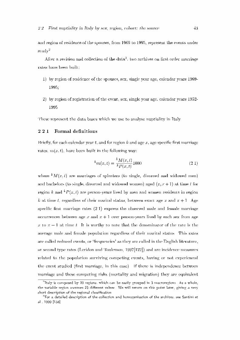
2.2. First nuptiality in Italy by sex, region, cohort: the source 43
and region of residence of the spouses, from 1969 to 1995, represent the events under
study2.
After a revision and collection of the data3, two archives on �rst order marriage
rates have been built:
1) by region of residence of the spouses, sex, single year age, calendar years 1969-
1995;
2) by region of registration of the event, sex, single year age, calendar years 1952-
1995.
These represent the data bases which we use to analyse nuptiality in Italy.
2.2.1 Formal de�nitions
Brie y, for each calendar year t, and for region k and age x, age speci�c �rst marriage
rates, m(x; t), have been built in the following way:
km(x; t) =kM(x; t)kP (x; t)
1000 (2.1)
where kM(x; t) are marriages of spinsters (to single, divorced and widowed men)
and bachelors (to single, divorced and widowed women) aged (x; x+1) at time t for
region k and kP (x; t) are person-years lived by men and women residents in region
k at time t, regardless of their marital status, between exact age x and x + 1. Age
speci�c �rst marriage rates (2.1) express the observed male and female marriage
occurrences between age x and x + 1 over person-years lived by each sex from age
x to x + 1 at time t. It is worthy to note that the denominator of the rate is the
average male and female population regardless of their marital status. This rates
are called reduced events, or `frequencies' as they are called in the English literature,
or second type rates (Leridon and Toulemon, 1997[122]) and are incidence measures
related to the population surviving competing events, having or not experienced
the event studied (�rst marriage, in this case). If there is independence between
marriage and these competing risks (mortality and migration) they are equivalent
2Italy is composed by 20 regions, which can be easily grouped in 3 macroregions. As a whole,
the variable region assumes 23 di�erent values. We will return on this point later, giving a very
short description of the regional classi�cation.3For a detailed description of the collection and homogenisation of the archives, see Santini et
al., 1999 [158].
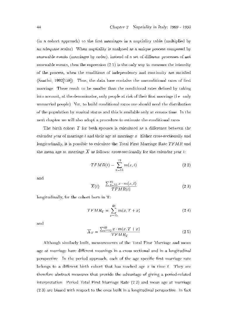
44 Chapter 2. Nuptiality in Italy: 1969 - 1995
(in a cohort approach) to the �rst marriages in a nuptiality table (multiplied by
an adequate scalar). When nuptiality is analysed as a unique process composed by
renewable events (marriages by order), instead of a set of di�erent processes of not
renewable events, then the expression (2.1) is the only way to measure the intensity
of the process, when the conditions of independency and continuity are satis�ed
(Santini, 1992[159]). Thus, the data base contains the unconditional rates of �rst
marriage. These result to be smaller than the conditional rates de�ned by taking
into account, at the denominator, only people at risk of their �rst marriage (i.e. only
unmarried people). Yet, to build conditional rates one should need the distribution
of the population by marital status and this is available only at census time. In the
next chapter we will also adopt a procedure to estimate the conditional rates.
The birth cohort T for both spouses is calculated as a di�erence between the
calendar year of marriage t and their age at marriage x. Either cross-sectionally and
longitudinally, it is possible to calculate the Total First Marriage Rate TFMR and
the mean age at marriage X as follows: cross-sectionally for the calendar year t:
TFMR(t) =49X
x=15
m(x; t) (2.2)
and
X(t) =
P49x=15 x �m(x; t)
TFMR(t)(2.3)
longitudinally, for the cohort born in T:
TFMRT =49X
x=15
m(x; T + x) (2.4)
and
XT =
P49x=15 x �m(x; T + x)
TFMRT(2.5)
Although similarly built, measurements of the Total First Marriage and mean
age at marriage have di�erent meanings in a cross sectional and in a longitudinal
perspective. In the period approach, each of the age speci�c �rst marriage rate
belongs to a di�erent birth cohort that has reached age x in time t. They are
therefore abstract measures that provide the advantage of giving a period-related
interpretation. Period Total First Marriage Rate (2.2) and mean age at marriage
(2.3) are biased with respect to the ones built in a longitudinal perspective. In fact
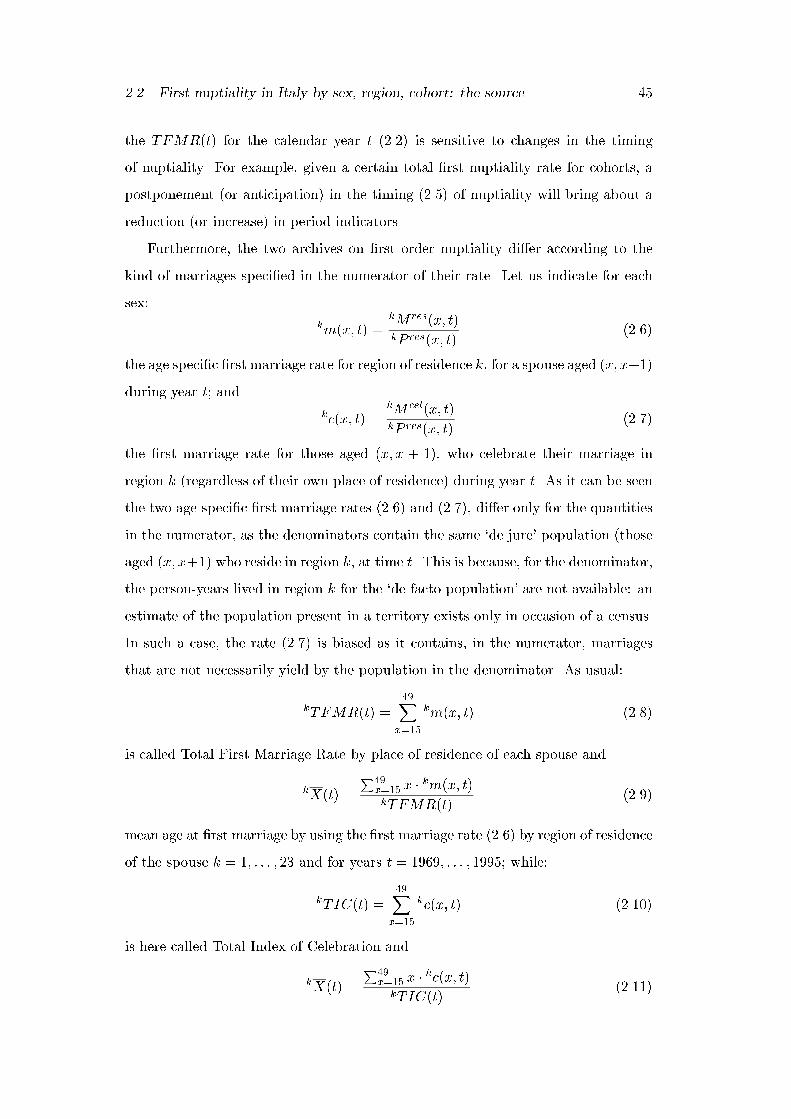
2.2. First nuptiality in Italy by sex, region, cohort: the source 45
the TFMR(t) for the calendar year t (2.2) is sensitive to changes in the timing
of nuptiality. For example, given a certain total �rst nuptiality rate for cohorts, a
postponement (or anticipation) in the timing (2.5) of nuptiality will bring about a
reduction (or increase) in period indicators.
Furthermore, the two archives on �rst order nuptiality di�er according to the
kind of marriages speci�ed in the numerator of their rate. Let us indicate for each
sex:
km(x; t) =kM res(x; t)kP res(x; t)
(2.6)
the age speci�c �rst marriage rate for region of residence k, for a spouse aged (x; x+1)
during year t; and
kc(x; t) =kM cel(x; t)kP res(x; t)
(2.7)
the �rst marriage rate for those aged (x; x + 1), who celebrate their marriage in
region k (regardless of their own place of residence) during year t. As it can be seen
the two age speci�c �rst marriage rates (2.6) and (2.7), di�er only for the quantities
in the numerator, as the denominators contain the same `de jure' population (those
aged (x; x+1) who reside in region k, at time t. This is because, for the denominator,
the person-years lived in region k for the `de facto population' are not available: an
estimate of the population present in a territory exists only in occasion of a census.
In such a case, the rate (2.7) is biased as it contains, in the numerator, marriages
that are not necessarily yield by the population in the denominator. As usual:
kTFMR(t) =49X
x=15
km(x; t) (2.8)
is called Total First Marriage Rate by place of residence of each spouse and
kX(t) =
P49x=15 x � km(x; t)kTFMR(t)
(2.9)
mean age at �rst marriage by using the �rst marriage rate (2.6) by region of residence
of the spouse k = 1; : : : ; 23 and for years t = 1969; : : : ; 1995; while:
kTIC(t) =49X
x=15
kc(x; t) (2.10)
is here called Total Index of Celebration and
kX(t) =
P49x=15 x � kc(x; t)
kTIC(t)(2.11)
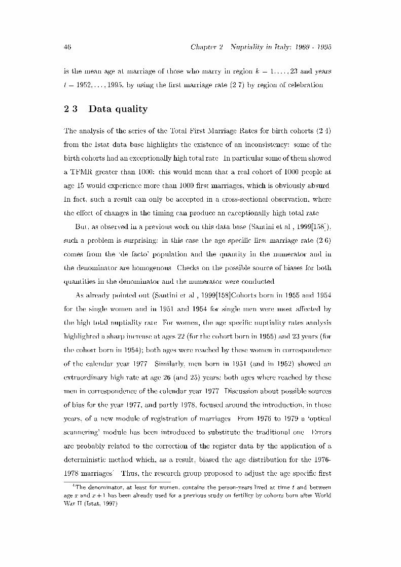
46 Chapter 2. Nuptiality in Italy: 1969 - 1995
is the mean age at marriage of those who marry in region k = 1; : : : ; 23 and years
t = 1952; : : : ; 1995, by using the �rst marriage rate (2.7) by region of celebration.
2.3 Data quality
The analysis of the series of the Total First Marriage Rates for birth cohorts (2.4)
from the Istat data base highlights the existence of an inconsistency: some of the
birth cohorts had an exceptionally high total rate. In particular some of them showed
a TFMR greater than 1000: this would mean that a real cohort of 1000 people at
age 15 would experience more than 1000 �rst marriages, which is obviously absurd.
In fact, such a result can only be accepted in a cross-sectional observation, where
the e�ect of changes in the timing can produce an exceptionally high total rate.
But, as observed in a previous work on this data base (Santini et al., 1999[158]),
such a problem is surprising: in this case the age speci�c �rst marriage rate (2.6)
comes from the `de facto' population and the quantity in the numerator and in
the denominator are homogenous. Checks on the possible source of biases for both
quantities in the denominator and the numerator were conducted.
As already pointed out (Santini et al., 1999[158]Cohorts born in 1955 and 1954
for the single women and in 1951 and 1954 for single men were most a�ected by
the high total nuptiality rate. For women, the age speci�c nuptiality rates analysis
highlighted a sharp increase at ages 22 (for the cohort born in 1955) and 23 years (for
the cohort born in 1954); both ages were reached by these women in correspondence
of the calendar year 1977. Similarly, men born in 1951 (and in 1952) showed an
extraordinary high rate at age 26 (and 25) years; both ages where reached by these
men in correspondence of the calendar year 1977. Discussion about possible sources
of bias for the year 1977, and partly 1978, focused around the introduction, in those
years, of a new module of registration of marriages. From 1976 to 1979 a `optical
scannering' module has been introduced to substitute the traditional one. Errors
are probably related to the correction of the register data by the application of a
deterministic method which, as a result, biased the age distribution for the 1976-
1978 marriages4. Thus, the research group proposed to adjust the age speci�c �rst
4The denominator, at least for women, contains the person-years lived at time t and between
age x and x+1 has been already used for a previous study on fertility by cohorts born after World
War II (Istat, 1997).
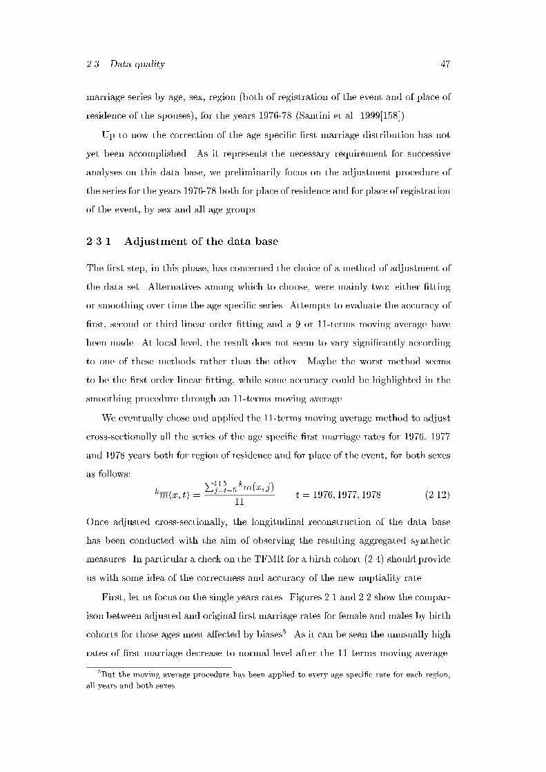
2.3. Data quality 47
marriage series by age, sex, region (both of registration of the event and of place of
residence of the spouses), for the years 1976-78 (Santini et al. 1999[158]).
Up to now the correction of the age speci�c �rst marriage distribution has not
yet been accomplished. As it represents the necessary requirement for successive
analyses on this data base, we preliminarily focus on the adjustment procedure of
the series for the years 1976-78 both for place of residence and for place of registration
of the event, by sex and all age groups.
2.3.1 Adjustment of the data base
The �rst step, in this phase, has concerned the choice of a method of adjustment of
the data set. Alternatives among which to choose, were mainly two: either �tting
or smoothing over time the age speci�c series. Attempts to evaluate the accuracy of
�rst, second or third linear order �tting and a 9 or 11-terms moving average have
been made. At local level, the result does not seem to vary signi�cantly according
to one of these methods rather than the other. Maybe the worst method seems
to be the �rst order linear �tting, while some accuracy could be highlighted in the
smoothing procedure through an 11-terms moving average.
We eventually chose and applied the 11-terms moving average method to adjust
cross-sectionally all the series of the age speci�c �rst marriage rates for 1976, 1977
and 1978 years both for region of residence and for place of the event, for both sexes
as follows:
km(x; t) =
Pt+5j=t�5
km(x; j)
11t = 1976; 1977; 1978 (2.12)
Once adjusted cross-sectionally, the longitudinal reconstruction of the data base
has been conducted with the aim of observing the resulting aggregated synthetic
measures. In particular a check on the TFMR for a birth cohort (2.4) should provide
us with some idea of the correctness and accuracy of the new nuptiality rate.
First, let us focus on the single years rates. Figures 2.1 and 2.2 show the compar-
ison between adjusted and original �rst marriage rates for female and males by birth
cohorts for those ages most a�ected by biases5. As it can be seen the unusually high
rates of �rst marriage decrease to normal level after the 11 terms moving average.
5But the moving average procedure has been applied to every age speci�c rate for each region,
all years and both sexes.
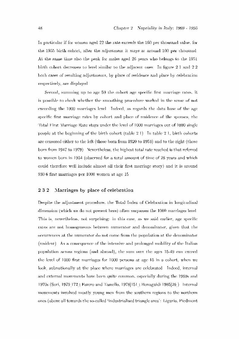
48 Chapter 2. Nuptiality in Italy: 1969 - 1995
In particular if for women aged 22 the rate exceeds the 160 per thousand value, for
the 1955 birth cohort, after the adjustment it stays at around 100 per thousand.
At the same time also the peak for males aged 26 years who belongs to the 1951
birth cohort decreases to level similar to the adjacent ones. In �gure 2.1 and 2.2
both cases of resulting adjustments, by place of residence and place by celebration
respectively, are displayed.
Second, summing up to age 50 the cohort age speci�c �rst marriage rates, it
is possible to check whether the smoothing procedure worked in the sense of not
exceeding the 1000 marriages level. Indeed, as regards the data base of the age
speci�c �rst marriage rates by cohort and place of residence of the spouses, the
Total First Marriage Rate stays under the level of 1000 marriages out of 1000 single
people at the beginning of the birth cohort (table 2.1). In table 2.1, birth cohorts
are censored either to the left (those born from 1920 to 1953) and to the right (those
born from 1947 to 1979). Nevertheless, the highest total rate reached is that referred
to women born in 1954 (observed for a total amount of time of 28 years and which
could therefore well include almost all their �rst marriage story) and it is around
930.6 �rst marriages per 1000 women at age 15.
2.3.2 Marriages by place of celebration
Despite the adjustment procedure, the Total Index of Celebration in longitudinal
dimension (which we do not present here) often surpasses the 1000 marriages level.
This is, nevertheless, not surprising: in this case, as we said earlier, age speci�c
rates are not homogeneous between numerator and denominator, given that the
occurrences at the numerator do not come from the population at the denominator
(resident). As a consequence of the intensive and prolonged mobility of the Italian
population across regions (and abroad), the sum over the ages 15-49 can exceed
the level of 1000 �rst marriages for 1000 persons at age 15 in a cohort, when we
look, subnationally at the place where marriages are celebrated. Indeed, internal
and external movements have been quite common, especially during the 1960s and
1970s (Sori, 1979[172]; Favero and Tassello, 1978[151]; Bonaguidi 1985[26]). Internal
movements involved mostly young men from the southern regions to the northern
ones (above all towards the so-called `industrialised triangle area': Liguria, Piedmont
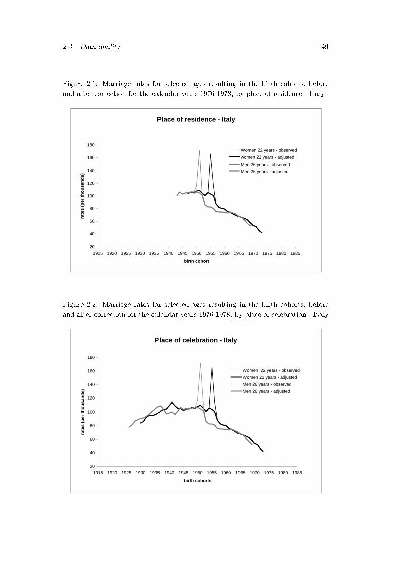
2.3. Data quality 49
Figure 2.1: Marriage rates for selected ages resulting in the birth cohorts, before
and after correction for the calendar years 1976-1978, by place of residence - Italy
Place of residence - Italy
20
40
60
80
100
120
140
160
180
1915 1920 1925 1930 1935 1940 1945 1950 1955 1960 1965 1970 1975 1980 1985
birth cohort
rate
s (p
er t
ho
usa
nd
s)
Women 22 years - observed
women 22 years - adjusted
Men 26 years - observed
Men 26 years - adjusted
Figure 2.2: Marriage rates for selected ages resulting in the birth cohorts, before
and after correction for the calendar years 1976-1978, by place of celebration - Italy
Place of celebration - Italy
20
40
60
80
100
120
140
160
180
1915 1920 1925 1930 1935 1940 1945 1950 1955 1960 1965 1970 1975 1980 1985
birth cohorts
rate
s (p
er t
ho
usa
nd
s)
Women 22 years - observed
Women 22 years - adjusted
Men 26 years - observed
Men 26 years - adjusted

50 Chapter 2. Nuptiality in Italy: 1969 - 1995
Table 2.1: Total First Marriage rates for the birth cohorts (censored), by sex and
region of residence - Italybirth
cohort NORTH CENTRE SOUTH ITALY NORTH CENTRE SOUTH ITALY
1920 1.0 1.1 1.5 1.2 1.2 1.6 1.6 1.41921 2.1 2.2 3.1 2.4 2.6 2.4 2.8 2.61922 3.5 3.2 4.7 3.8 4.5 4.3 5.3 4.71923 6.4 6.8 7.8 6.9 7.2 7.0 7.5 7.31924 8.4 8.7 11.0 9.3 9.7 9.1 10.4 9.81925 10.3 11.7 13.6 11.6 12.2 11.6 12.7 12.31926 12.7 12.7 17.2 14.2 15.2 14.1 16.8 15.51927 14.5 15.2 19.8 16.3 18.2 16.8 20.2 18.61928 16.8 17.0 22.9 18.8 21.8 19.2 25.5 22.51929 19.6 19.6 27.9 22.3 26.3 24.3 29.8 27.01930 22.4 23.9 30.7 25.4 31.5 29.0 38.0 33.11931 26.2 25.0 35.3 28.9 36.4 34.7 45.2 38.91932 28.7 28.4 39.9 32.3 42.9 40.0 52.5 45.41933 33.3 31.3 44.6 36.7 52.3 49.9 64.7 55.81934 38.4 36.0 52.5 42.6 62.3 59.7 77.9 66.81935 43.4 41.7 56.5 47.3 74.2 71.9 93.9 80.01936 48.1 48.6 64.9 53.6 91.7 90.7 113.4 98.41937 57.4 55.8 75.2 62.8 113.0 110.9 140.3 121.21938 68.9 65.7 89.7 74.8 145.8 150.1 182.2 157.81939 81.1 82.3 106.5 89.4 183.6 193.0 230.7 199.91940 100.9 102.9 128.8 110.2 238.5 256.0 290.9 258.21941 126.3 130.2 163.0 138.7 318.8 336.9 380.1 341.11942 160.1 166.9 204.7 175.5 381.9 410.2 454.0 409.41943 207.6 210.5 252.1 222.5 484.1 519.2 553.6 512.31944 267.8 273.4 317.4 284.5 586.1 631.4 633.4 608.91945 343.8 355.0 389.0 360.9 662.9 683.7 726.4 687.01946 458.2 457.1 475.7 463.2 758.8 816.7 794.1 780.61947 550.0 552.4 548.2 548.9 803.3 848.3 853.8 828.21948 658.7 656.7 630.2 647.0 832.0 877.7 883.8 858.01949 742.4 739.6 716.9 731.7 850.6 885.1 908.7 877.11950 812.8 816.8 793.3 806.0 851.1 891.8 906.1 878.11951 853.3 868.9 851.2 855.4 855.7 899.4 923.6 888.51952 869.7 870.3 878.7 873.9 838.4 872.9 904.7 869.11953 891.2 895.9 915.7 902.7 819.9 851.7 899.4 854.91954 891.5 911.3 930.6 912.1 802.2 839.0 869.5 834.11955 886.0 893.5 918.4 902.2 790.1 824.5 873.5 828.01956 857.4 865.8 901.6 878.0 786.9 814.5 856.8 818.41957 830.5 852.0 879.4 855.3 768.8 786.1 837.9 798.01958 821.9 828.5 878.1 846.9 758.9 779.4 831.0 789.91959 815.2 819.1 865.5 837.4 745.8 767.0 818.0 777.11960 807.5 809.2 863.2 831.4 729.2 742.0 808.1 761.61961 802.8 796.5 855.8 824.2 684.4 705.2 770.2 720.91962 781.0 784.1 847.4 809.6 649.3 669.9 746.3 689.81963 758.2 756.1 829.1 787.7 609.3 624.3 707.4 649.01964 720.7 729.0 806.5 757.7 561.5 572.3 666.6 602.81965 676.7 669.4 766.1 712.2 496.9 504.2 609.0 540.21966 628.9 619.9 726.1 667.1 426.0 422.9 535.5 466.51967 560.9 555.7 685.4 610.7 342.7 334.2 453.5 383.21968 495.2 485.1 633.3 549.8 266.4 254.8 372.3 304.91969 413.4 401.8 562.8 471.8 191.9 182.5 280.5 224.41970 327.2 319.9 484.9 389.7 124.4 113.8 203.0 153.01971 246.2 236.2 400.8 307.3 76.7 68.7 136.2 98.61972 170.3 164.5 312.2 227.1 43.0 40.7 86.8 60.01973 111.0 108.4 234.3 161.4 22.9 23.0 50.8 34.31974 65.9 67.5 165.6 108.1 11.4 11.3 27.6 18.21975 36.3 37.4 109.7 67.9 5.3 5.4 14.2 9.11976 18.5 20.6 65.8 39.5 2.2 2.4 6.5 4.11977 7.9 8.1 31.6 18.5 0.8 0.7 2.4 1.51978 0.8 1.6 5.1 2.9 0.1 0.1 0.3 0.21979 0.2 0.4 1.6 0.9 0.0 . 0.0 0.0
WOMEN MEN
2.3. Data quality 51
and Lombardy). Moreover, it should be observed the emerging role of some regions
(for instance Umbria) to their religious `attractiveness' for the spread of sanctuaries.
External movements were directed towards European countries and were also
seasonal movements without a changing of the residence: this implies that men
turned frequently back to Italy to marry. We should also note the existence up
to the beginning of the 1960s, of a fascist law that did not allow for transferring
the residence to a new one, unless a certi�cate of a regular job in the new city was
shown. But, despite of the mobility of the population, marriages are often celebrated
in a region di�erent from that where one resides. Regions with high Total Index
of Celebration are mainly the southern ones and Umbria (in the Centre). We can
hypothesise the following: although men migrated to the North, they returned to
marry in the South, probably because their native regions still represented their
pools (next chapters will shed lights on this hypothesis). The case of Umbria can be
slightly di�erent: we can hypothesise that in this region, maybe, a high attraction
is played by the presence of lots of religious sanctuaries spread in all the territory.
Despite the fact that it cannot be used to somehow measure the total propensity to
marry for a real cohort, the Total Index of Celebration can still provide a measure
of the attractiveness of the place of celebration.
Let us compare the age speci�c �rst marriage rates in a year t for those aged
(x; x+1), who celebrate their marriage in region k (regardless of their own place of
residence) (2.7) and those who reside in a region k (2.6).
What can be observed from a comparison between the two measures, given that
the denominators are constants, is that, when (2.7) is greater than (2.6), then surely
spouses who contract their marriages in region k are more than those who there
also reside. In this case it is possible to say that region k attracts marriages from
people who normally reside elsewhere. This is often the case when, for example the
partners live in two di�erent regions and they necessarily have to decide where to
marry. Normally, in Italy, marriage is uxorilocal and therefore it is highly likely that
the groom, for the marriage celebration, moves to the place where the bride lives
and resides. Another reason could be that, because of the existence of their own
network of families and relatives in the place where they bore, migrant men return
to marry in their place of origin. For instance, a southern man, migrated to the
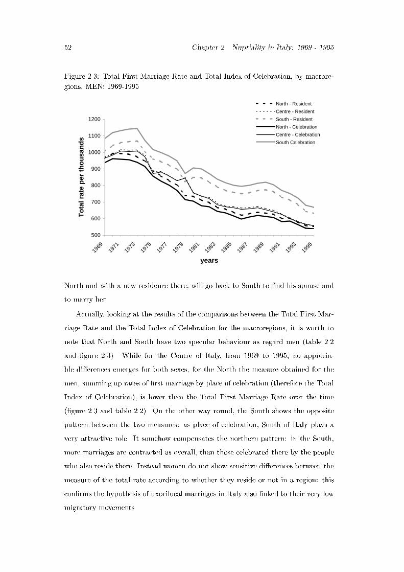
52 Chapter 2. Nuptiality in Italy: 1969 - 1995
Figure 2.3: Total First Marriage Rate and Total Index of Celebration, by macrore-
gions, MEN: 1969-1995
500
600
700
800
900
1000
1100
1200
1969
1971
1973
1975
1977
1979
1981
1983
1985
1987
1989
1991
1993
1995
years
To
tal r
ate
per
th
ou
san
ds
North - Resident
Centre - Resident
South - Resident
North - Celebration
Centre - Celebration
South Celebration
North and with a new residence there, will go back to South to �nd his spouse and
to marry her.
Actually, looking at the results of the comparisons between the Total First Mar-
riage Rate and the Total Index of Celebration for the macroregions, it is worth to
note that North and South have two specular behaviour as regard men (table 2.2
and �gure 2.3). While for the Centre of Italy, from 1969 to 1995, no apprecia-
ble di�erences emerges for both sexes, for the North the measure obtained for the
men, summing up rates of �rst marriage by place of celebration (therefore the Total
Index of Celebration), is lower than the Total First Marriage Rate over the time
(�gure 2.3 and table 2.2). On the other way round, the South shows the opposite
pattern between the two measures: as place of celebration, South of Italy plays a
very attractive role. It somehow compensates the northern pattern: in the South,
more marriages are contracted as overall, than those celebrated there by the people
who also reside there. Instead women do not show sensitive di�erences between the
measure of the total rate according to whether they reside or not in a region: this
con�rms the hypothesis of uxorilocal marriages in Italy also linked to their very low
migratory movements.
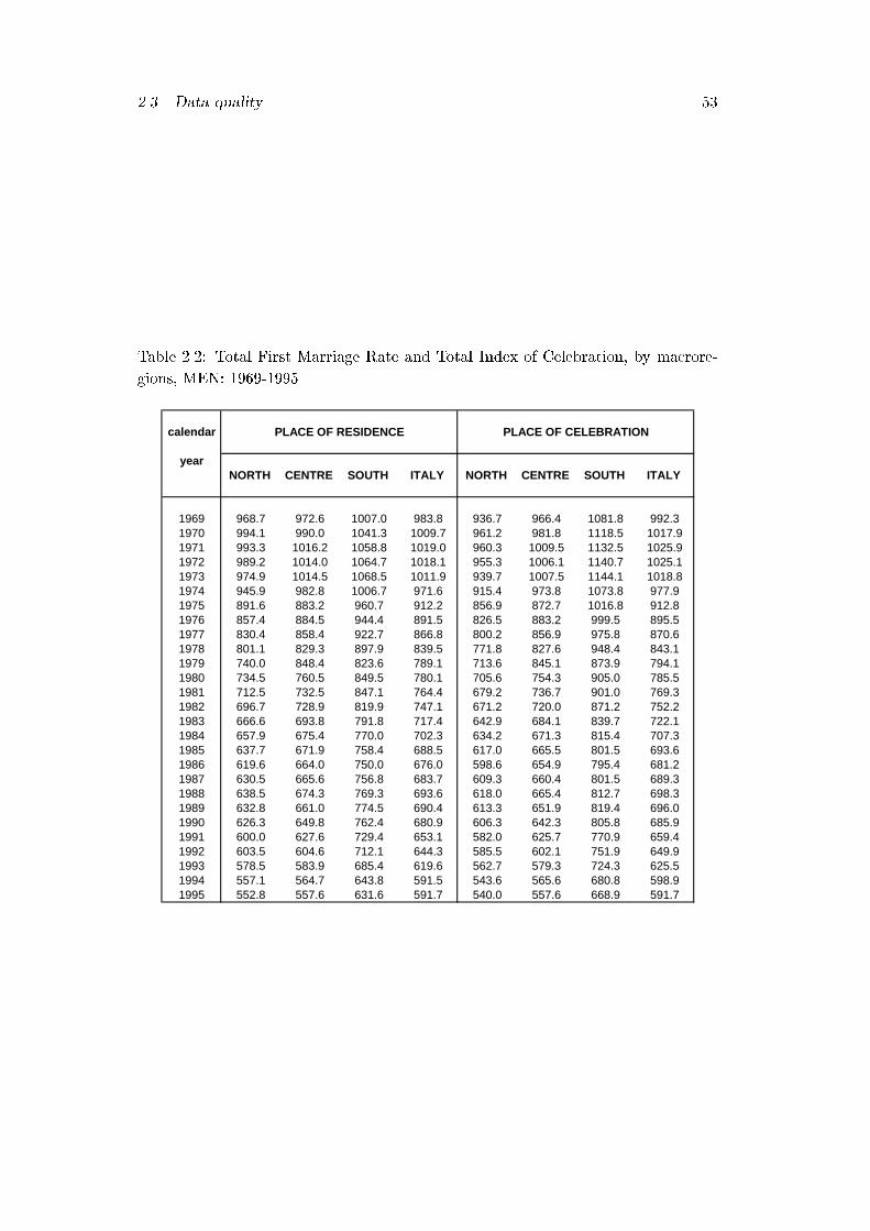
2.3. Data quality 53
Table 2.2: Total First Marriage Rate and Total Index of Celebration, by macrore-
gions, MEN: 1969-1995
calendar
yearNORTH CENTRE SOUTH ITALY NORTH CENTRE SOUTH ITALY
1969 968.7 972.6 1007.0 983.8 936.7 966.4 1081.8 992.31970 994.1 990.0 1041.3 1009.7 961.2 981.8 1118.5 1017.91971 993.3 1016.2 1058.8 1019.0 960.3 1009.5 1132.5 1025.91972 989.2 1014.0 1064.7 1018.1 955.3 1006.1 1140.7 1025.11973 974.9 1014.5 1068.5 1011.9 939.7 1007.5 1144.1 1018.81974 945.9 982.8 1006.7 971.6 915.4 973.8 1073.8 977.91975 891.6 883.2 960.7 912.2 856.9 872.7 1016.8 912.81976 857.4 884.5 944.4 891.5 826.5 883.2 999.5 895.51977 830.4 858.4 922.7 866.8 800.2 856.9 975.8 870.61978 801.1 829.3 897.9 839.5 771.8 827.6 948.4 843.11979 740.0 848.4 823.6 789.1 713.6 845.1 873.9 794.11980 734.5 760.5 849.5 780.1 705.6 754.3 905.0 785.51981 712.5 732.5 847.1 764.4 679.2 736.7 901.0 769.31982 696.7 728.9 819.9 747.1 671.2 720.0 871.2 752.21983 666.6 693.8 791.8 717.4 642.9 684.1 839.7 722.11984 657.9 675.4 770.0 702.3 634.2 671.3 815.4 707.31985 637.7 671.9 758.4 688.5 617.0 665.5 801.5 693.61986 619.6 664.0 750.0 676.0 598.6 654.9 795.4 681.21987 630.5 665.6 756.8 683.7 609.3 660.4 801.5 689.31988 638.5 674.3 769.3 693.6 618.0 665.4 812.7 698.31989 632.8 661.0 774.5 690.4 613.3 651.9 819.4 696.01990 626.3 649.8 762.4 680.9 606.3 642.3 805.8 685.91991 600.0 627.6 729.4 653.1 582.0 625.7 770.9 659.41992 603.5 604.6 712.1 644.3 585.5 602.1 751.9 649.91993 578.5 583.9 685.4 619.6 562.7 579.3 724.3 625.51994 557.1 564.7 643.8 591.5 543.6 565.6 680.8 598.91995 552.8 557.6 631.6 591.7 540.0 557.6 668.9 591.7
PLACE OF RESIDENCE PLACE OF CELEBRATION
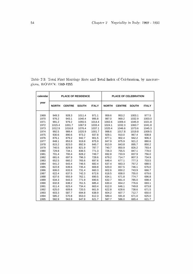
54 Chapter 2. Nuptiality in Italy: 1969 - 1995
Table 2.3: Total First Marriage Rate and Total Index of Celebration, by macrore-
gions, WOMEN: 1969-1995
calendar
yearNORTH CENTRE SOUTH ITALY NORTH CENTRE SOUTH ITALY
1969 949.3 928.3 1011.4 971.1 959.6 953.2 1003.1 977.51970 976.2 943.1 1040.4 995.8 987.0 969.2 1032.9 1003.01971 991.2 979.2 1055.5 1014.4 1002.6 1009.4 1045.9 1021.81972 1015.4 1001.7 1067.9 1033.4 1024.1 1032.3 1063.7 1041.81973 1012.9 1016.8 1076.4 1037.1 1020.4 1046.6 1073.6 1045.31974 992.5 989.4 1020.9 1001.7 998.6 1017.8 1019.8 1009.51975 930.6 890.6 973.2 937.8 929.1 910.0 967.4 938.81976 876.1 879.2 942.7 901.5 877.1 902.4 942.2 906.31977 848.1 853.9 919.8 875.9 847.9 875.9 921.2 880.61978 815.2 823.0 892.9 845.7 813.9 843.8 895.7 850.21979 740.5 829.9 821.9 787.7 740.7 850.9 826.2 793.41980 729.8 734.1 836.5 771.3 726.3 755.5 847.1 778.01981 701.4 700.4 828.2 749.7 692.8 733.9 837.9 756.01982 681.6 697.9 796.3 728.6 679.2 714.7 807.3 734.91983 652.5 660.2 765.6 697.6 648.4 677.1 777.3 703.51984 641.2 643.4 746.5 682.4 637.4 663.3 757.2 688.51985 622.8 639.6 735.4 669.8 620.0 657.5 746.1 676.01986 606.0 633.9 731.4 660.3 602.6 650.2 743.9 666.71987 622.4 637.5 742.3 672.6 618.5 658.0 755.0 679.61988 637.6 655.9 762.1 690.5 634.1 671.8 774.7 696.81989 634.3 643.3 771.9 690.6 632.7 661.4 785.0 698.41990 632.8 638.2 761.5 685.4 630.4 654.2 776.6 693.11991 611.4 623.4 734.4 663.4 612.0 646.1 749.8 673.81992 625.0 609.6 720.5 661.9 622.8 628.6 738.6 671.51993 603.3 587.7 694.8 638.9 604.2 607.7 712.7 650.01994 585.2 570.8 653.0 612.3 589.4 591.8 671.0 625.01995 582.9 563.9 647.8 621.7 587.7 586.0 665.4 621.7
PLACE OF RESIDENCE PLACE OF CELEBRATION
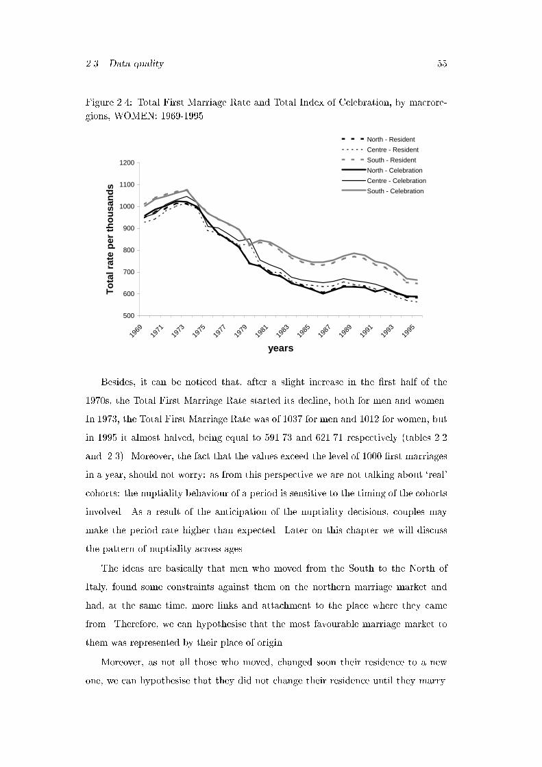
2.3. Data quality 55
Figure 2.4: Total First Marriage Rate and Total Index of Celebration, by macrore-
gions, WOMEN: 1969-1995
500
600
700
800
900
1000
1100
1200
1969
1971
1973
1975
1977
1979
1981
1983
1985
1987
1989
1991
1993
1995
years
To
tal r
ate
per
th
ou
san
ds
North - Resident
Centre - Resident
South - Resident
North - Celebration
Centre - Celebration
South - Celebration
Besides, it can be noticed that, after a slight increase in the �rst half of the
1970s, the Total First Marriage Rate started its decline, both for men and women.
In 1973, the Total First Marriage Rate was of 1037 for men and 1012 for women, but
in 1995 it almost halved, being equal to 591.73 and 621.71 respectively (tables 2.2
and 2.3). Moreover, the fact that the values exceed the level of 1000 �rst marriages
in a year, should not worry: as from this perspective we are not talking about `real'
cohorts: the nuptiality behaviour of a period is sensitive to the timing of the cohorts
involved. As a result of the anticipation of the nuptiality decisions, couples may
make the period rate higher than expected. Later on this chapter we will discuss
the pattern of nuptiality across ages.
The ideas are basically that men who moved from the South to the North of
Italy, found some constraints against them on the northern marriage market and
had, at the same time, more links and attachment to the place where they came
from. Therefore, we can hypothesise that the most favourable marriage market to
them was represented by their place of origin.
Moreover, as not all those who moved, changed soon their residence to a new
one, we can hypothesise that they did not change their residence until they marry.
56 Chapter 2. Nuptiality in Italy: 1969 - 1995
If this is the case, then the attachment towards the place of origin can be strong,
even in terms of the marriage market.
Bearing in mind the characteristics of the nuptiality rates by place of celebration,
we shall, by now on, consider only the data base of the nuptiality rates by region of
residence. The basic assumptions that support this choice are:
� rates that come from the resident population (2.6) are homogeneous in their nu-
merator and denominator, and longitudinally they hold a demographic mean-
ing;
� the place of residence can be assumed as a proxy of the future place of residence,
at least for men.
An open question regards the role of the place of origin and its socio-cultural im-
portance in marital choices, but this is going to be investigated in the next chapters
(by using survey data) as a problem of homogamy by place of origin.
2.4 Patterns of Italian marriage
Even though data have been computed at regional level, in this part we just look
at the national or macro-regional level, given that the purpose of this chapter is not
to provide a detailed di�erential analysis at the regional level, but to investigate
more general shifts in marriage behaviour over time and, partly, across cohorts.
Sometimes, we will attempt to go deeper in the territorial analysis6. Again, we will
analyse only the data base of marriage rates by place of residence of the spouses at
the time of the occurrence.
2.4.1 Cross-sectional analysis
The analysis of nuptiality patterns is conducted by looking at the cross-sectional
levels of the Total First Nuptiality Rates and of the mean age at marriage for both
sexes from 1969 to 1995. As already seen in tables 2.2 and 2.3 and �gures 2.3 and 2.4,
6Italian regions can be broadly divided in three macroregions: North, Centre and South. In
particular, Piedmont, Valle d'Aosta, Lombardy, Liguria, Trentino AltoAdige, Veneto, Friuli Venezia
Giulia and Emilia Romagna belong to the North; Tuscany, Umbria, Marches, Lazio belong to the
Centre; and Abruzzo, Molise, Campania, Apulia, Basilicata, Calabria, Sicily and Sardinia form the
South of Italy.
2.4. Patterns of Italian marriage 57
in more than 30 years there has been a general decline in the Total First Marriage
Rates for both sexes. In particular, up to 1974 there is a slight increase in the total
rate, while after that year a phase of decline becomes clear. During the �rst half
of the 1970s, Total First Marriage Rate is higher than 1000, as results from the
anticipatory behaviour of some cohorts. (Later we are going to investigate cohorts,
as well.) The highest levels of Total First Marriage Rate are reached in the South,
especially by the 1973 female �rst marriages. After that year, marriage behaviour
dramatically shifted.
In thirty years the TFMR in Italy almost halved. In particular, at the begin-
ning of the 1970s we should expect more than a thousand �rst marriages from an
hypothetical cohort of 1000 men at age 15, if they experienced, at all the ages, the
same rates observed that year (table 2.2). In 1995, the number of total marriages
expected to be contracted by an hypothetical cohort of 1000 is 591.7 marriages for
men (table 2.2) and 621.7 for women (table 2.3). From 1971, when we observe the
highest rate for men for Italy as a whole, to 1995, the total rate for 1000 men in the
North has decreased of about 44%, in the Centre of about 45% and in the South of
about 40%. For women, instead, the decrease from the 1973 level was around 42, 45
and 40% respectively in the North, Centre and South of Italy. It should be observed
that the decline has been shortly interrupted in 1979, when the Centre showed a
small rise, and the South a deeper reduction, and at the very end of the 1980s, when
a slight recover of marriages appears.
As regards mean age at marriage, a general behaviour can be envisaged also at
macroregional level (Figure 2.5). In particular, if at the national level age at �rst
marriage has passed from 23.6 years in 1969 to 26.2 in 1995, for brides, and from 27.0
to 29.1, for grooms, the increase has been quite heterogeneous for the macroregions.
For instance, women in the North have delayed their �rst marriage from age 23.7
to 26.7 (3.0 years), those in the Centre have passed from age 23.6 to 26.9 (with the
highest increase in the age at �rst marriage: 3.3 years), while those in the South
have showed a slight delay from age 23.5 to 25.4 (1.9 years of delay only). In the
same way, northern men postponed the age at their �rst marriage from age 27.0 to
29.4 (therefore a delay of 2.4 years), those in the central regions from 27.0 to 29.7
(with an increase of 2.7) and those in the southern ones from 27.0 to 28.6 years (only
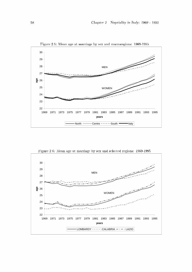
58 Chapter 2. Nuptiality in Italy: 1969 - 1995
Figure 2.5: Mean age at marriage by sex and macroregions: 1969-1995
22
23
24
25
26
27
28
29
30
1969 1971 1973 1975 1977 1979 1981 1983 1985 1987 1989 1991 1993 1995
years
age
North Centre South Italy
MEN
WOMEN
Figure 2.6: Mean age at marriage by sex and selected regions: 1969-1995
22
23
24
25
26
27
28
29
30
1969 1971 1973 1975 1977 1979 1981 1983 1985 1987 1989 1991 1993 1995
years
age
LOMBARDY CALABRIA LAZIO
MEN
WOMEN

2.4. Patterns of Italian marriage 59
1.5 years of delay in almost thirty years).
Overall, both sexes show a phase of decline from the beginning of the period up
to the �rst half of the 1970s (�gure 2.5). But then, women since 1980 and men since
1982, started to increase their mean ages at �rst marriage up to 1995. In particular,
southern Italy still shows the lowest age at �rst marriage than wherever in the
country, while in central Italy women have the highest age at �rst marriage. Mean
age at marriage for men deserves a note: up to 1982, men resident in the southern
regions showed the highest average age at marriage, and those in the northern regions
the lowest, but then a shift takes place and, as a result, men in the South have the
lowest age at �rst marriage than all the other Italians.
In the last thirty years, there has been a growing di�erentiation of the marital
behaviour, at least as regard the mean age at marriage, at a territorial level, espe-
cially for women. While in 1969 the mean age was homogenous between spouses in
the North, Centre or South of Italy, in 1995 the age di�erence at �rst marriage is
around 1.5 years between brides in the Centre and in the South, and about 1.1 years
between grooms resident in the Centre and those resident in the South.
If we look at the di�erentiation between regions with regard to the ages of their
spouses, we can say that it roughly goes from more than 3 years in 1969, more
precisely from 3.3 in the North to 3.4 in the Centre and 3.5 in the South) to 2.8 in
the North and in the Centre, to 3.2 in the South.
Taking into account three regions, Lombardy, Lazio and Calabria as representa-
tives of North, Centre and South of Italy respectively, we should notice the widening
pattern among women in their age at �rst marriage. While men's patterns get closer,
being characterised by a faster shift upwards of Lazio and Lombardy average ages,
women's levels get increasingly distant. In particular, the pattern of Calabria seems
to move upward more slowly than the Lazio and Lombardy ones.
Over the last thirty years the shift upwards of the mean ages at marriage has also
entailed a rearrangement of the distribution of the regions according to their average
ages. Tables 2.4 and 2.5 classify each region according to the position occupied at
the beginning and at the end of the period. As regard women the major jump
upward in the age at �rst marriage is made by Emilia Romagna (from 1969 to 1995
it goes from position 14 to 5), while the biggest jump backward is made by Campania

60 Chapter 2. Nuptiality in Italy: 1969 - 1995
Table 2.4: Italian regions by decreasing order of the mean ages at marriage in 1969
and 1995 - WOMEN1969 mean position 1995 mean position
age ageSardinia 24.94 1 Liguria 27.16 1Trentino Alto Adige 24.80 2 Friuli Venezia Giulia 27.09 2Liguria 24.16 3 Lazio 27.05 3Campania 23.87 4 Sardinia 27.05 4Lombardy 23.80 5 Emilia Romagna 27.04 5Lazio 23.73 6 Tuscany 26.89 6Tuscany 23.62 7 Trentino Alto Adige 26.81 7Veneto 23.60 8 Lombardy 26.62 8Apulia 23.58 9 Umbria 26.60 9Friuli Venezia Giulia 23.51 10 Marches 26.59 10Marches 23.47 11 Veneto 26.49 11Piedmont 23.46 12 Piedmont 26.33 12Abruzzo 23.41 13 Abruzzo 26.05 13Emilia Romagna 23.39 14 Valle d'aosta 26.04 14Umbria 23.28 15 Molise 26.03 15Valle d'aosta 23.19 16 Basilicata 25.99 16Sicily 23.00 17 Apulia 25.54 17Calabria 22.93 18 Campania 25.24 18Basilicata 22.90 19 Calabria 25.18 19Molise 22.62 20 Sicily 24.96 20
Table 2.5: Italian regions by decreasing order of the mean ages at marriage in 1969
and 1995 - MEN1969 mean position 1995 mean position
age ageSardinia 28.81 1 Sardinia 30.04 1Trentino Alto Adige 28.45 2 Liguria 30.02 2Marches 27.40 3 Friuli Venezia Giulia 30.01 3Liguria 27.37 4 Trentino Alto Adige 29.95 4Abruzzo 27.16 5 Marches 29.82 5Lazio 27.11 6 Lazio 29.79 6Lombardy 27.09 7 Emilia Romagna 29.66 7Sicily 27.03 8 Tuscany 29.52 8Calabria 27.01 9 Umbria 29.52 9Friuli Venezia Giulia 27.00 10 Lombardy 29.38 10Umbria 26.99 11 Molise 29.34 11Campania 26.93 12 Veneto 29.31 12Veneto 26.89 13 Abruzzo 29.22 13Basilicata 26.89 14 Basilicata 29.18 14Tuscany 26.78 15 Piedmont 29.10 15Piedmont 26.75 16 Valle d'aosta 29.04 16Emilia Romagna 26.67 17 Calabria 28.85 17Apulia 26.67 18 Apulia 28.43 18Molise 26.43 19 Campania 28.31 19Valle d'aosta 26.40 20 Sicily 28.31 20
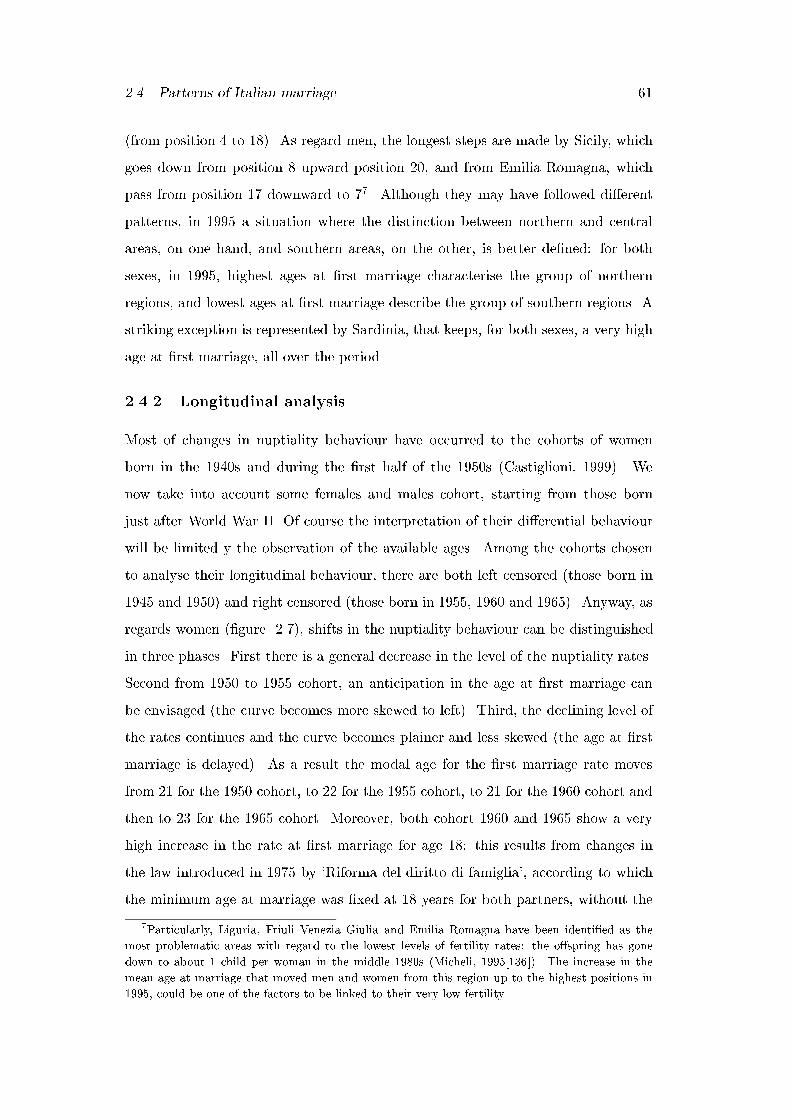
2.4. Patterns of Italian marriage 61
(from position 4 to 18). As regard men, the longest steps are made by Sicily, which
goes down from position 8 upward position 20, and from Emilia Romagna, which
pass from position 17 downward to 77. Although they may have followed di�erent
patterns, in 1995 a situation where the distinction between northern and central
areas, on one hand, and southern areas, on the other, is better de�ned: for both
sexes, in 1995, highest ages at �rst marriage characterise the group of northern
regions, and lowest ages at �rst marriage describe the group of southern regions. A
striking exception is represented by Sardinia, that keeps, for both sexes, a very high
age at �rst marriage, all over the period.
2.4.2 Longitudinal analysis
Most of changes in nuptiality behaviour have occurred to the cohorts of women
born in the 1940s and during the �rst half of the 1950s (Castiglioni, 1999). We
now take into account some females and males cohort, starting from those born
just after World War II. Of course the interpretation of their di�erential behaviour
will be limited y the observation of the available ages. Among the cohorts chosen
to analyse their longitudinal behaviour, there are both left censored (those born in
1945 and 1950) and right censored (those born in 1955, 1960 and 1965). Anyway, as
regards women (�gure 2.7), shifts in the nuptiality behaviour can be distinguished
in three phases. First there is a general decrease in the level of the nuptiality rates.
Second from 1950 to 1955 cohort, an anticipation in the age at �rst marriage can
be envisaged (the curve becomes more skewed to left). Third, the declining level of
the rates continues and the curve becomes plainer and less skewed (the age at �rst
marriage is delayed). As a result the modal age for the �rst marriage rate moves
from 21 for the 1950 cohort, to 22 for the 1955 cohort, to 21 for the 1960 cohort and
then to 23 for the 1965 cohort. Moreover, both cohort 1960 and 1965 show a very
high increase in the rate at �rst marriage for age 18: this results from changes in
the law introduced in 1975 by `Riforma del diritto di famiglia', according to which
the minimum age at marriage was �xed at 18 years for both partners, without the
7Particularly, Liguria, Friuli Venezia Giulia and Emilia Romagna have been identi�ed as the
most problematic areas with regard to the lowest levels of fertility rates: the o�spring has gone
down to about 1 child per woman in the middle 1980s (Micheli, 1995[136]). The increase in the
mean age at marriage that moved men and women from this region up to the highest positions in
1995, could be one of the factors to be linked to their very low fertility.
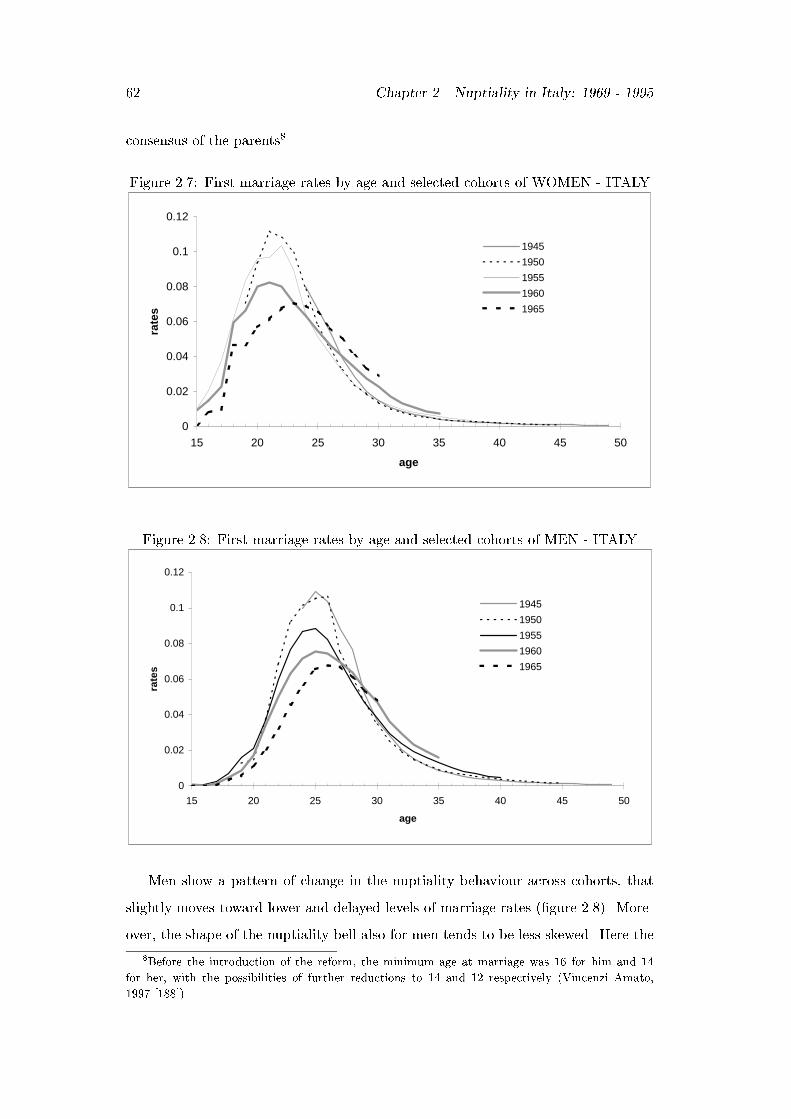
62 Chapter 2. Nuptiality in Italy: 1969 - 1995
consensus of the parents8.
Figure 2.7: First marriage rates by age and selected cohorts of WOMEN - ITALY
0
0.02
0.04
0.06
0.08
0.1
0.12
15 20 25 30 35 40 45 50
age
rate
s
1945
1950
1955
1960
1965
Figure 2.8: First marriage rates by age and selected cohorts of MEN - ITALY
0
0.02
0.04
0.06
0.08
0.1
0.12
15 20 25 30 35 40 45 50
age
rate
s
1945
1950
1955
1960
1965
Men show a pattern of change in the nuptiality behaviour across cohorts, that
slightly moves toward lower and delayed levels of marriage rates (�gure 2.8). More-
over, the shape of the nuptiality bell also for men tends to be less skewed. Here the
8Before the introduction of the reform, the minimum age at marriage was 16 for him and 14
for her, with the possibilities of further reductions to 14 and 12 respectively (Vincenzi Amato,
1997 [188]).
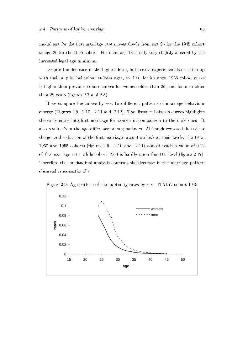
2.4. Patterns of Italian marriage 63
modal age for the �rst marriage rate moves slowly from age 25 for the 1945 cohort
to age 26 for the 1965 cohort. For men, age 18 is only very slightly a�ected by the
increased legal age minimum.
Despite the decrease in the highest level, both sexes experience also a catch up
with their nuptial behaviour at later ages, so that, for instance, 1965 cohort curve
is higher than previous cohort curves for women older than 26, and for men older
than 29 years (�gures 2.7 and 2.8).
If we compare the curves by sex, two di�erent patterns of marriage behaviour
emerge (Figures 2.9, 2.10, 2.11 and 2.12). The distance between curves highlights
the early entry into �rst marriage for women in comparison to the male ones. It
also results from the age di�erence among partners. Although censored, it is clear
the general reduction of the �rst marriage rates if we look at their levels: the 1945,
1950 and 1955 cohorts (�gures 2.9, 2.10 and 2.11) almost reach a value of 0.12
of the marriage rate, while cohort 1960 is hardly upon the 0.08 level (�gure 2.12).
Therefore the longitudinal analysis con�rms the decrease in the marriage pattern
observed cross-sectionally.
Figure 2.9: Age pattern of the nuptiality rates by sex - ITALY: cohort 1945
0
0.02
0.04
0.06
0.08
0.1
0.12
15 20 25 30 35 40 45 50
age
rate
s
women
men
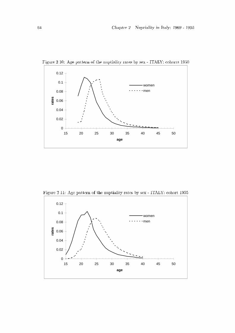
64 Chapter 2. Nuptiality in Italy: 1969 - 1995
Figure 2.10: Age pattern of the nuptiality rates by sex - ITALY: cohorts 1950
0
0.02
0.04
0.06
0.08
0.1
0.12
15 20 25 30 35 40 45 50
age
rate
s
women
men
Figure 2.11: Age pattern of the nuptiality rates by sex - ITALY: cohort 1955
0
0.02
0.04
0.06
0.08
0.1
0.12
15 20 25 30 35 40 45 50
age
rate
s
women
men
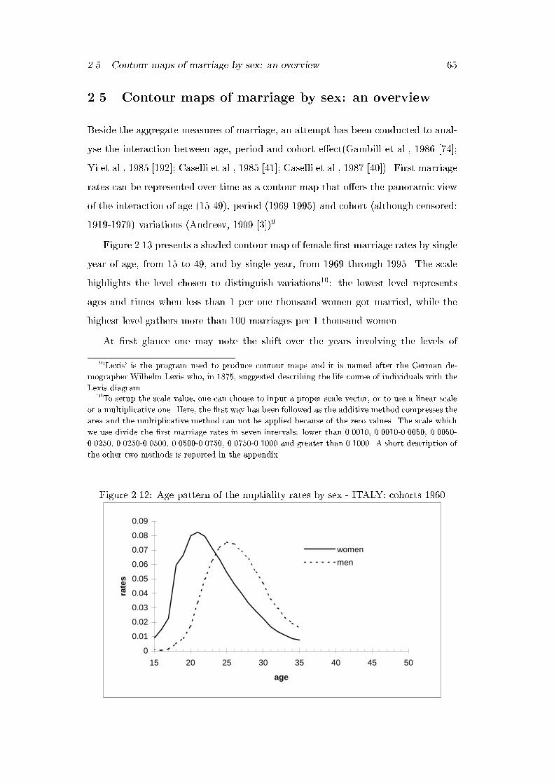
2.5. Contour maps of marriage by sex: an overview 65
2.5 Contour maps of marriage by sex: an overview
Beside the aggregate measures of marriage, an attempt has been conducted to anal-
yse the interaction between age, period and cohort e�ect(Gambill et al., 1986 [74];
Yi et al., 1985 [192]; Caselli et al., 1985 [41]; Caselli et al., 1987 [40]). First marriage
rates can be represented over time as a contour map that o�ers the panoramic view
of the interaction of age (15-49), period (1969-1995) and cohort (although censored:
1919-1979) variations (Andreev, 1999 [3])9.
Figure 2.13 presents a shaded contour map of female �rst marriage rates by single
year of age, from 15 to 49, and by single year, from 1969 through 1995. The scale
highlights the level chosen to distinguish variations10: the lowest level represents
ages and times when less than 1 per one thousand women got married, while the
highest level gathers more than 100 marriages per 1 thousand women.
At �rst glance one may note the shift over the years involving the levels of
9`Lexis' is the program used to produce contour maps and it is named after the German de-
mographer Wilhelm Lexis who, in 1875, suggested describing the life course of individuals with the
Lexis diagram.10To setup the scale value, one can choose to input a proper scale vector, or to use a linear scale
or a multiplicative one. Here, the �rst way has been followed as the additive method compresses the
area and the multiplicative method can not be applied because of the zero values. The scale which
we use divide the �rst marriage rates in seven intervals: lower than 0.0010, 0.0010-0.0050, 0.0050-
0.0250, 0.0250-0.0500, 0.0500-0.0750, 0.0750-0.1000 and greater than 0.1000. A short description of
the other two methods is reported in the appendix.
Figure 2.12: Age pattern of the nuptiality rates by sex - ITALY: cohorts 1960
0
0.01
0.02
0.03
0.04
0.05
0.06
0.07
0.08
0.09
15 20 25 30 35 40 45 50
age
rate
s
women
men
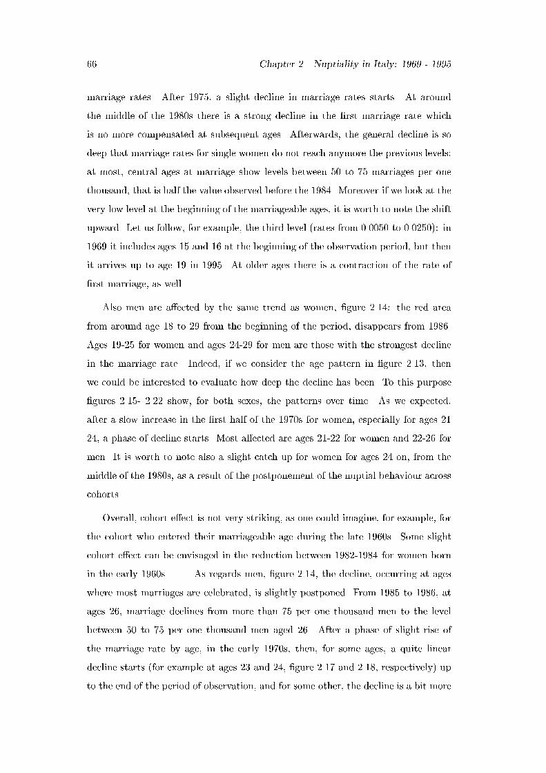
66 Chapter 2. Nuptiality in Italy: 1969 - 1995
marriage rates. After 1975, a slight decline in marriage rates starts. At around
the middle of the 1980s there is a strong decline in the �rst marriage rate which
is no more compensated at subsequent ages. Afterwards, the general decline is so
deep that marriage rates for single women do not reach anymore the previous levels:
at most, central ages at marriage show levels between 50 to 75 marriages per one
thousand, that is half the value observed before the 1984. Moreover if we look at the
very low level at the beginning of the marriageable ages, it is worth to note the shift
upward. Let us follow, for example, the third level (rates from 0.0050 to 0.0250): in
1969 it includes ages 15 and 16 at the beginning of the observation period, but then
it arrives up to age 19 in 1995. At older ages there is a contraction of the rate of
�rst marriage, as well.
Also men are a�ected by the same trend as women, �gure 2.14: the red area
from around age 18 to 29 from the beginning of the period, disappears from 1986.
Ages 19-25 for women and ages 24-29 for men are those with the strongest decline
in the marriage rate. Indeed, if we consider the age pattern in �gure 2.13, then
we could be interested to evaluate how deep the decline has been. To this purpose
�gures 2.15- 2.22 show, for both sexes, the patterns over time. As we expected,
after a slow increase in the �rst half of the 1970s for women, especially for ages 21
24, a phase of decline starts. Most a�ected are ages 21-22 for women and 22-26 for
men. It is worth to note also a slight catch up for women for ages 24 on, from the
middle of the 1980s, as a result of the postponement of the nuptial behaviour across
cohorts.
Overall, cohort e�ect is not very striking, as one could imagine, for example, for
the cohort who entered their marriageable age during the late 1960s. Some slight
cohort e�ect can be envisaged in the reduction between 1982-1984 for women born
in the early 1960s. As regards men, �gure 2.14, the decline, occurring at ages
where most marriages are celebrated, is slightly postponed. From 1985 to 1986, at
ages 26, marriage declines from more than 75 per one thousand men to the level
between 50 to 75 per one thousand men aged 26. After a phase of slight rise of
the marriage rate by age, in the early 1970s, then, for some ages, a quite linear
decline starts (for example at ages 23 and 24, �gure 2.17 and 2.18, respectively) up
to the end of the period of observation, and for some other, the decline is a bit more

2.5. Contour maps of marriage by sex: an overview 67
Figure 2.13: Contour maps of �rst marriage rates, WOMEN - ITALY, 1969-1995
0.0010
0.0050
0.0250
0.0500
0.0750
0.1000
1969 1975 1980 1985 1990 1996
15
20
25
30
35
40
45
49
years
age
Figure 2.14: Contour maps of �rst marriage rates, MEN - ITALY: 1969-1995
0.0010
0.0050
0.0250
0.0500
0.0750
0.1000
1969 1975 1980 1985 1990 1996
15
20
25
30
35
40
45
50
years
age
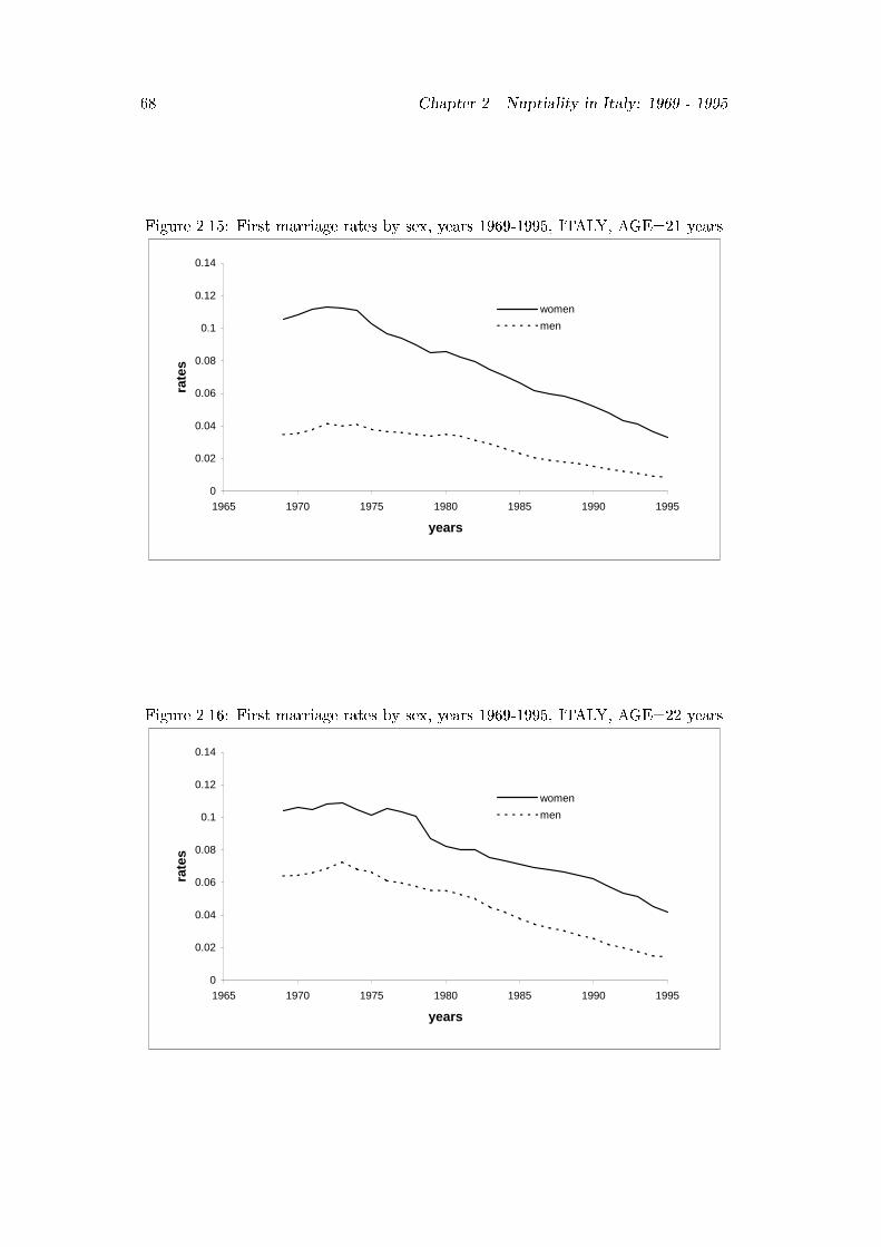
68 Chapter 2. Nuptiality in Italy: 1969 - 1995
Figure 2.15: First marriage rates by sex, years 1969-1995, ITALY, AGE=21 years
0
0.02
0.04
0.06
0.08
0.1
0.12
0.14
1965 1970 1975 1980 1985 1990 1995
years
rate
s
women
men
Figure 2.16: First marriage rates by sex, years 1969-1995, ITALY, AGE=22 years
0
0.02
0.04
0.06
0.08
0.1
0.12
0.14
1965 1970 1975 1980 1985 1990 1995
years
rate
s
women
men
2.5. Contour maps of marriage by sex: an overview 69
Figure 2.17: First marriage rates by sex, years 1969-1995, ITALY, AGE=23 years
0
0.02
0.04
0.06
0.08
0.1
0.12
0.14
1965 1970 1975 1980 1985 1990 1995
years
rate
s
women
men
Figure 2.18: First marriage rates by sex, years 1969-1995, ITALY, AGE=24 years
0
0.02
0.04
0.06
0.08
0.1
0.12
0.14
1965 1970 1975 1980 1985 1990 1995
years
rate
s
women
men
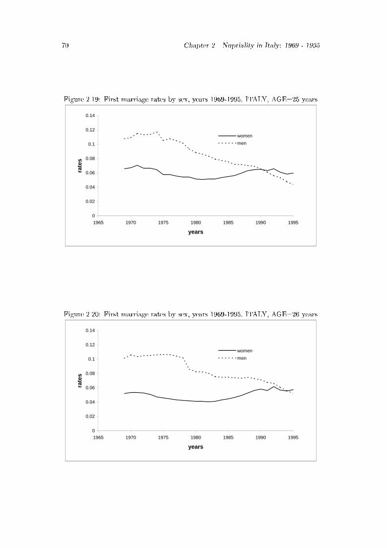
70 Chapter 2. Nuptiality in Italy: 1969 - 1995
Figure 2.19: First marriage rates by sex, years 1969-1995, ITALY, AGE=25 years
0
0.02
0.04
0.06
0.08
0.1
0.12
0.14
1965 1970 1975 1980 1985 1990 1995
years
rate
s
women
men
Figure 2.20: First marriage rates by sex, years 1969-1995, ITALY, AGE=26 years
0
0.02
0.04
0.06
0.08
0.1
0.12
0.14
1965 1970 1975 1980 1985 1990 1995
years
rate
s
women
men

2.5. Contour maps of marriage by sex: an overview 71
Figure 2.21: First marriage rates by sex, years 1969-1995, ITALY, AGE=27 years
0
0.02
0.04
0.06
0.08
0.1
0.12
0.14
1965 1970 1975 1980 1985 1990 1995
years
rate
s
women
men
Figure 2.22: First marriage rates by sex, years 1969-1995, ITALY, AGE=28 years
0
0.02
0.04
0.06
0.08
0.1
0.12
0.14
1965 1970 1975 1980 1985 1990 1995
years
rate
s
women
men
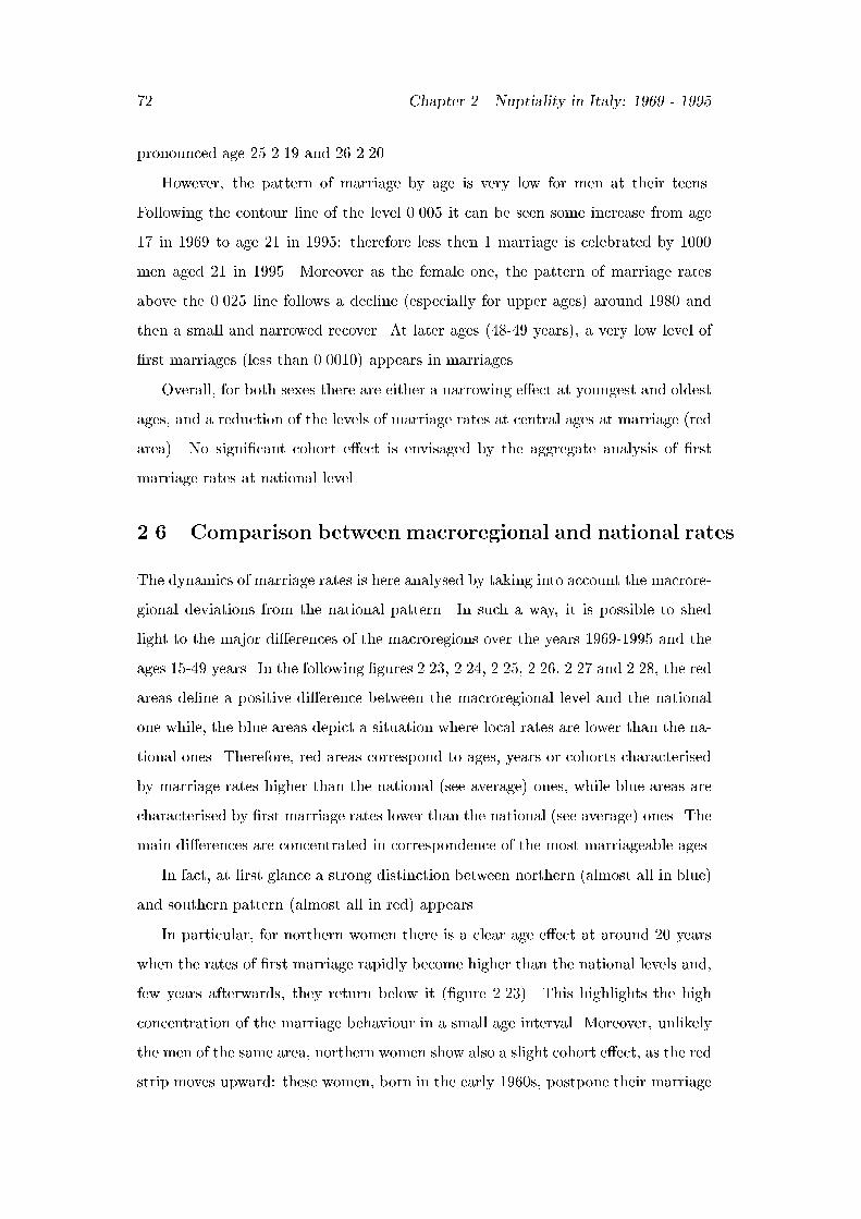
72 Chapter 2. Nuptiality in Italy: 1969 - 1995
pronounced age 25 2.19 and 26 2.20.
However, the pattern of marriage by age is very low for men at their teens.
Following the contour line of the level 0.005 it can be seen some increase from age
17 in 1969 to age 21 in 1995: therefore less then 1 marriage is celebrated by 1000
men aged 21 in 1995. Moreover as the female one, the pattern of marriage rates
above the 0.025 line follows a decline (especially for upper ages) around 1980 and
then a small and narrowed recover. At later ages (48-49 years), a very low level of
�rst marriages (less than 0.0010) appears in marriages.
Overall, for both sexes there are either a narrowing e�ect at youngest and oldest
ages, and a reduction of the levels of marriage rates at central ages at marriage (red
area). No signi�cant cohort e�ect is envisaged by the aggregate analysis of �rst
marriage rates at national level.
2.6 Comparison between macroregional and national rates
The dynamics of marriage rates is here analysed by taking into account the macrore-
gional deviations from the national pattern. In such a way, it is possible to shed
light to the major di�erences of the macroregions over the years 1969-1995 and the
ages 15-49 years. In the following �gures 2.23, 2.24, 2.25, 2.26, 2.27 and 2.28, the red
areas de�ne a positive di�erence between the macroregional level and the national
one while, the blue areas depict a situation where local rates are lower than the na-
tional ones. Therefore, red areas correspond to ages, years or cohorts characterised
by marriage rates higher than the national (see average) ones, while blue areas are
characterised by �rst marriage rates lower than the national (see average) ones. The
main di�erences are concentrated in correspondence of the most marriageable ages.
In fact, at �rst glance a strong distinction between northern (almost all in blue)
and southern pattern (almost all in red) appears.
In particular, for northern women there is a clear age e�ect at around 20 years
when the rates of �rst marriage rapidly become higher than the national levels and,
few years afterwards, they return below it (�gure 2.23). This highlights the high
concentration of the marriage behaviour in a small age interval. Moreover, unlikely
the men of the same area, northern women show also a slight cohort e�ect, as the red
strip moves upward: these women, born in the early 1960s, postpone their marriage

2.6. Comparison between macroregional and national rates 73
at later ages more than elsewhere in the country (see also �gure 2.7). Men in the
North experience higher rates at �rst marriage than all the Italians only up to the
beginning of the 1980s, but then they quickly shift their behaviour, marrying later
(�gure 2.24 and 2.8). A specular situation emerges for the South, where almost all
the surfaces are red (�gures 2.27 and 2.28), therefore signaling higher rates of �rst
marriage. In particular the South shows �rst marriage rates higher than the national
ones both at early and at older ages. On the contrary, for the marriageable ages a
blue strip toward upper ages divide the female pattern. Men show a blue spot up
the early 1980s.
The Centre of Italy depicts a more variegated situations. An age e�ect appears
for both sexes at around 20 years for women (�gure 2.25) and 24-25 years for men
(�gure 2.26). Below those ages the rates of the central regions are lower than the
national level and the contrary happens for the rates in the red strip above it. A
slight increase in the threshold of deviation from the national level appears for the
cohorts born in the early 1960s. A period e�ect can be envisaged for the year 1979
when, with respect to the adjacent years, the rates are higher than the national ones.
Understanding the factors a�ecting this period e�ect needs more in depth analysis.
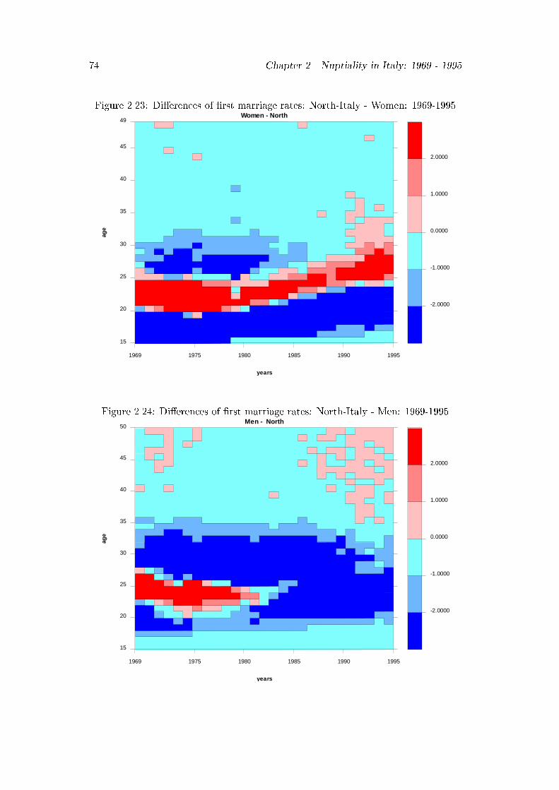
74 Chapter 2. Nuptiality in Italy: 1969 - 1995
Figure 2.23: Di�erences of �rst marriage rates: North-Italy - Women: 1969-1995
-2.0000
-1.0000
0.0000
1.0000
2.0000
1969 1975 1980 1985 1990 1995
15
20
25
30
35
40
45
49Women - North
years
age
Figure 2.24: Di�erences of �rst marriage rates: North-Italy - Men: 1969-1995
-2.0000
-1.0000
0.0000
1.0000
2.0000
1969 1975 1980 1985 1990 1995
15
20
25
30
35
40
45
50Men - North
years
age

2.6. Comparison between macroregional and national rates 75
Figure 2.25: Di�erences of �rst marriage rates: Centre-Italy - Women: 1969-1995
-2.0000
-1.0000
0.0000
1.0000
2.0000
1969 1975 1980 1985 1990 1996
15
20
25
30
35
40
45
50Women - Centre
years
age
Figure 2.26: Di�erences of �rst marriage rates: Centre-Italy - Men: 1969-1995
-2.0000
-1.0000
0.0000
1.0000
2.0000
1969 1975 1980 1985 1990 1996
15
20
25
30
35
40
45
50Men - Centre
years
age
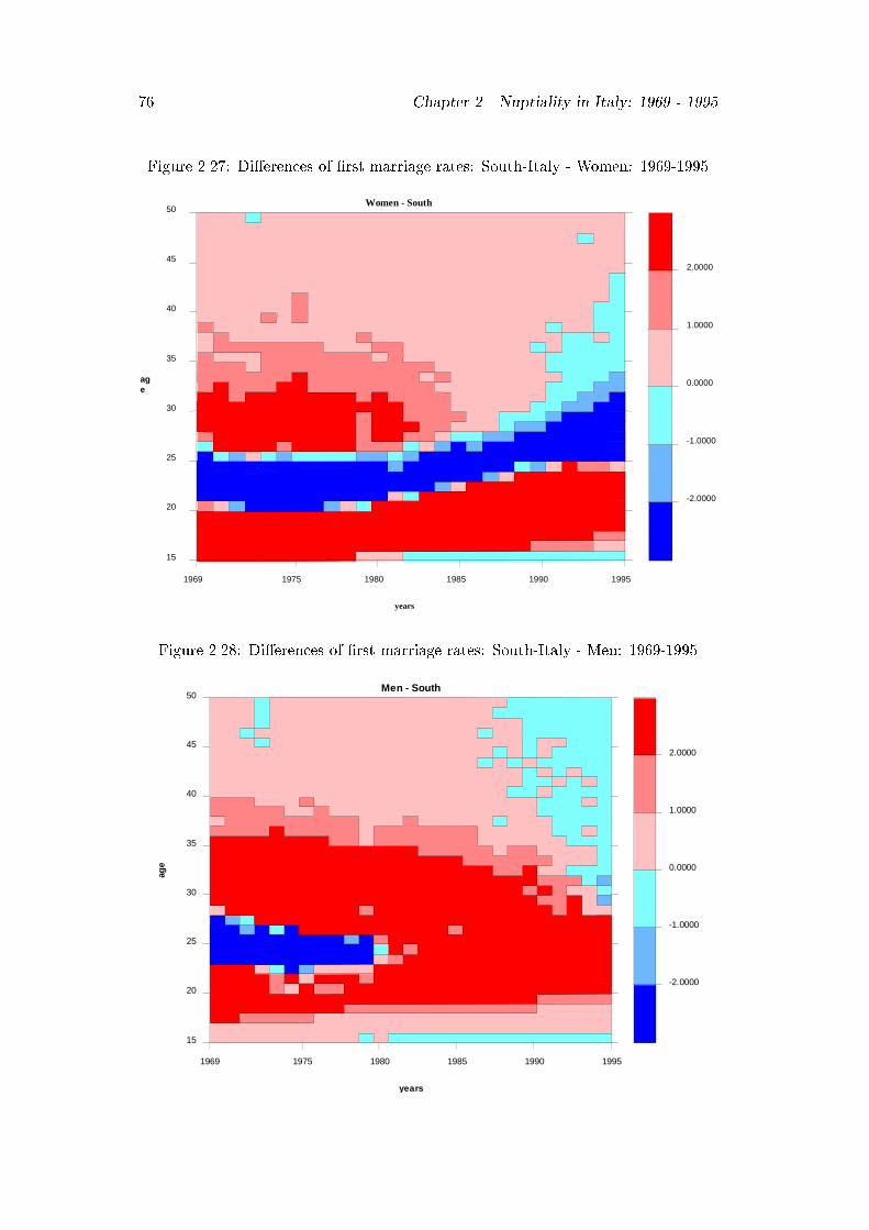
76 Chapter 2. Nuptiality in Italy: 1969 - 1995
Figure 2.27: Di�erences of �rst marriage rates: South-Italy - Women: 1969-1995
-2.0000
-1.0000
0.0000
1.0000
2.0000
1969 1975 1980 1985 1990 1995
15
20
25
30
35
40
45
50Women - South
years
age
Figure 2.28: Di�erences of �rst marriage rates: South-Italy - Men: 1969-1995
-2.0000
-1.0000
0.0000
1.0000
2.0000
1969 1975 1980 1985 1990 1995
15
20
25
30
35
40
45
50Men - South
years
age
2.7. Summary 77
2.7 Summary
Brie y, in this chapter we described the nuptiality data base available in Italy for
both sexes and we adjusted the age speci�c �rst marriage rates for the years 1976-
78. On the adjusted data base by place of residence of the spouses, occurrence
and intensity of marriage have been described mainly at the macroregional level
and only sporadically the focus is on the regional level. The period under study is
characterised by a steady reduction: over 30 years Total First Marriage Rate has
halved. The mean age at marriage declined for both sexes from 1969 up to the �rst
half of the 1970s. Since 1980, women and, since 1982, men experienced a constant
increase in the age at �rst marriage and a growing territorial di�erentiation. The
cohort analysis looked at the pattern of the age speci�c �rst marriage rates by sex:
decrease of the levels of the rates, postponement of the modal values (but for women
there is a slight anticipation for the 1955-1960 cohorts), and decrease in the skewness
around them are the main features of the transformations occurred across cohorts.
Contour maps are here applied to study nuptiality at glance: they provide us
with a useful tool in highlighting the major shifts occurred in the last 30 years to
the Italian marriage behaviour. Although it remains still hard to disentangle cohort,
period and age-related e�ects, the contour maps analysis does not reveal strong
cohort e�ects, at least at national level for the period under study: all cohorts are
progressively involved in the process of postponement of nuptiality. Maybe a slight
e�ect could be seen for the cohort of women born in the early 1960s. The period
e�ect which lower the rates between 1980 and 1985 for both sexes is quite evident.
As regard age, one should note the reduction in the level of nuptiality between 20-
24 years for women, and 23-29 for men, and the slight movement upward of the
nuptiality rate, as a result of the postponement of marriage. Lastly, the decline in
marriage observed at very young ages, at least for women is the consequence of the
modi�cation by law of the minimum age at marriage.

78 Chapter 2. Nuptiality in Italy: 1969 - 1995
Chapter 3
Measures of the Imbalance on
the Marriage Market
3.1 Introduction
In this chapter we focus on what is known in literature as the marriage market.
The search of a partner is strictly linked with the availability of the eligibles of the
opposite sex. In the �rst chapter we have already introduced the concept of marriage
squeeze as the e�ect on marriage behaviour of the imbalances between the number
of men and women in their prime ages at marriage. Marriage squeezes are typically
a consequence of di�erential cohort size.
In the next sections, after a brief review of the most used measures introduced in
the literature, some indices of the marriage squeeze to Italian nuptiality tables. In
particular, three measures of the imbalance between the sexes at marriageable ages
will be applied to the cross-sectional tables for the years 1969-1995. Unfortunately,
the unavailability of completed nuptiality tables by birth cohorts does not allow to
measure this imbalance longitudinally.
The aim of the chapter is to analyse the Italian marriage market and to study
whether deep changes in natality observed over time, since World War II, may have
played a role in the transition to marriage for both sexes. We study Italy both in its
baby-boom period and its baby-bust period. The latter is particularly interesting
because it made Italy one of the countries with the lowest fertility ever observed. It
seems worthwhile to measure the impact of structural constraints on nuptiality and
to interpret changes in nuptiality also as the result of the imbalance between the
sexes.
79
80 Chapter 3. Measures of the Imbalance on the Marriage Market
This chapter provides also an aggregate time-dependent measure of the imbal-
ance on the marriage market to be used as a proxy of the constraints played by the
population structure resulting from its frequent shifts in birth patterns from World
War II onward. As the analysis will be conducted by region of residence (the data
base used in the previous chapter), a tentative interpretation of the consequences on
marriage opportunities, of the di�erentials between sexes of internal migration will
be presented.
In particular, after brie y reminding the goals pursued in literature for studying
the marriage market conditions and some of its implications (section 3.2), in section
3.3 we present an overview of the measures introduced by scholars. These can be
broadly divided between those that use sex-ratios (section 3.3.1) and those who
focus on the two-sex problem approach (section 3.3.2). Besides these, also other
new indices of the marriage market imbalance have been introduced here (section
3.3.3). All these measures will be applied to two one-sex nuptiality tables which
will then be build to this purpose (see appendix). Section 3.4 presents the outcomes
of the application of the measures of the squeeze (the one introduced by Schoen in
1983 and the two new alternatives proposed here) to the trends over time in Italy
and section 3.5 focus on the regional pattern, giving space to some discussion and
comments on the intertwined roles of marriage and migration (sections 3.5.1, 3.5.2
and 3.6).
3.2 Marriage market and marriage squeeze: trends over
time
As we said in the �rst chapter, the term marriage squeeze was introduced in 1959
(Glick et al., 1963[83]) to refer to the situation created by the baby boom in the
United States. The rapid increase in the birth rates then meant a shortage of eligible
men and a `squeeze' for women at their marriageable ages. The authors speculated
that some of the excess women would never marry while some others would marry
men who were younger or older than men they would have married in case of absence
of the baby boom. Evidence showed, few years afterwards, that, during the period
1951-1978, changes in the age sex distribution of the young population caused a
3.2. Marriage market and marriage squeeze: trends over time 81
decrease of 1.5 years in the mean age at marriage for men and an increase of about
1.5 years in the mean age at marriage for women, besides an increase in the dispersion
of the age at marriage, especially for women (Schoen, 1983[164]).
Many scholars have argued that the marriage squeeze has several other far-
reaching social implications. As an example, according to the economic point of
view expressed by Herr and Grossbard-Shechtman (1981[100]), the marriage squeeze
reduced the proportion of U.S. females who would have married in the 1960s and
1970s and lowered the `compensation' that men were obliged to pay women for their
traditional roles. They argued that, together with the availability of contraception
the marriage squeeze fostered the spread of the Women's Liberation Movements.
Moreover, an appreciable deviation from a balanced sex ratio has been interpreted
as one of the factors a�ecting the relationships between sexes as well as family and
other social institutions (Guttentag and Secord, 1983[92]). A shortage of women,
emphasises traditional sex roles, because men who want to get married are required
a greater commitment to the union. Conversely, when there is a surplus of women,
traditional aspects of marriage and the family play a minor role and divorce and
births out-of-wedlock become more widespread.
Fluctuations in fertility caused by baby booms and baby busts gave rise to very
important changes in the number of live births in Italy. Moreover internal migra-
tion, immigration, and emigration have shaped the size of the eligible population in
signi�cant ways. It is conceivable that large uctuations had a signi�cant impact,
some decades later, on the marriage market, creating marriage squeezes, and they
may also have been partially responsible for changes in the transition to marriage.
There has however not been any systematic attempt to analyse the dynamics of
the marriage market and marriage squeezes in the light of long-term uctuations in
birth rates.
The understanding of the marriage squeeze is linked to the manifestations of
two-sex population dynamics given that men and women reciprocally interact in
the process of matching. The discussion here is heavily based on Schoen 1988[166],
1983[164].
The analysis of nuptiality as well as fertility, should take into account that the
male and female marriage rates in each reciprocal preference are in uenced by the
82 Chapter 3. Measures of the Imbalance on the Marriage Market
age-sex composition of the population. Thus the observed marriage rates re ect
the interaction of the underlying preferences and the age-sex composition of that
population. This is one of the most important distinctions to make between marriage
or fertility rates on one side and mortality, divorce, migration, or other demographic
rates on the other side: the latter can be basically seen as determined by a �xed set of
underlying propensities that are independent of the composition of the population1.
Let us assume that in an hypothetical population men typically marry women
two years younger. A rise in the annual number of births of that population, will
bring about a marriage squeeze for women: men will be looking for brides among
larger cohorts of women born some years earlier, while women must look for grooms
among the smaller cohorts born some years before. If the population has instead
experienced a substantial decline in the annual number of births, the same process
would operate, but it would be the men who would be caught in a marriage squeeze.
Brie y, the mating problem arises from the following set of circumstances:
� men and women marry on the average at di�erent ages2,
� the number of births uctuates from year to year.
Basically, the equilibrium between the sexes in a marriage market depends on
(McDonald, 1995[133]):
� Sex Ratio at birth and the survival male/female ratio from birth to age at
marriage, if marriage takes place always at the same age;
� age structure, which is a function of the variation of births across years, if
marriage takes place at di�erent ages. Two cases can be distinguished: on
one hand we may have a stationary population where the number of births
N = constant, on the other hand a non stationary population (where N 6=
constant), whose case is more complex.
1For example, the probability that a person exact age x will die, depends only on the force of
mortality at that age, while the probability that a men exact age x will marry a woman exact age
y depends on the (x; y) marriage preference, the male population at exact age x and the female
population at exact age y.2The marriage market re ects the e�ects of the age-sex structure of a population, but also the
existence of social norms that somehow regulate the proper age at marriage. In particular, social
norms may also prescribe a range of acceptable ages or even acceptable di�erences between the ages
of partners (Billari, Micheli, 1999[19]).
3.3. Measure of the marriage squeeze 83
The way to measure quantitative imbalances between the men and women on the
marriage market is not unique. Many scholars proposed, according to their aims,
alternative measures but a general agreement does not exist, yet.
3.3 Measure of the marriage squeeze
The measures introduced in the literature for studying marriage market conditions
can be broadly divided between two categories: those that use sex-ratios and those
that focus on the two-sex approach. Let us �rst discuss both sets of measures and
then propose two simple new measures.
3.3.1 Sex Ratios
The most common way to measure the marriage squeeze is by means of a sex ratio,
which is usually expressed as the number of men for every 100 eligible women. A
very simple measure of the marriage market is the sex ratio for selected age groups
determined on the basis of the cross-classi�ed ages at marriage for men and women,
as for example:
I1 = 100M25�29
F20�24(3.1)
Often, men in a given age group have been compared to women in a smaller and
some years earlier age group, re ecting the empirical di�erences between partners'
ages. Of course, having age groups of the same width does not take into account
the fact that the female age distribution of marriage is normally more concentrated
around the mode than the male distribution and that there may be variations in the
timing of the process.
An alternative measure has been introduced by Akers (1967[1]), who de�nes
the following index of the marriage squeeze as weighted ratio of men who marry
women aged y over women aged y, where the weights at each age approximate the
probability of marriage at that age. The weights for the index proposed by Akers
are �rst marriages of women aged 15-24 and men aged 15-29. According to Akers,
these ranges include those ages at which most women marry and the ages of most
of the men whom they marry (more than 80% in both cases, Akers, 1967 [1]).
84 Chapter 3. Measures of the Imbalance on the Marriage Market
I2 =
P24y=15Ay
P29x=15B
yxP
mxP24
y=15AyPfy
(3.2)
in which: P is the population, x is the age of male, y is the age of female, Byx is
the proportion of females marrying at age y who marry men of age x, and Ay is
the proportion of all females that marry at age y, taken from a (period) nuptiality
table. Note that for any given age of females, the relative supply of marriageable
males may be given by the following expression:
iy =
P29x=15B
yxP
mx
Pfy
where in the numerator there are men who marry women aged y and in the
denominator there are women aged y. The author attributes the increase in the age
at marriage and in marriage rates, observed in United States in the 1960s, to the
dynamics of the age-sex population composition. The disproportions in the number
of males and females of a given age at their �rst marriage were due to the fact that
more females were born in the baby-boom period (after World War II: June 1946 -
July 1947) than males a few years earlier (July 1944 - June 1945). As a consequence,
American women in the 1960s faced a marriage squeeze.
To measure the impact on sex roles in the United States of the female marriage
squeeze (the shift in the sex ratio at eligible ages which took place in the late
1950s and early 1960s), the contraceptive revolution (which began in the 1960s),
and the women's liberation movement Heer and Grossbard-Shechtman (1981[100])
introduce two di�erent indexes. Their basic idea is to compare men and women in
an age interval of the same width for both sexes. In particular, the age intervals
were chosen such that the midpoint of the male group, 23.0 years, was very close to
the median age at �rst marriage for men during the period that starts in the early
1960s and ends in 1975; while the midpoint of the female group, 20.5 years, was very
close to that of women at the beginning of this period. Therefore, as a �rst measure,
they introduce the ratio of males aged 19.50-26.49 to females aged 17.00-23.99 as:
I3 =M19:50�26:49
F17:00�23:99| {z }7�year period surrounding the median age at first marriage for each sex
(3.3)
As Akers (1967[1]) previously pointed out, there is more than one way to measure
marriage squeeze and therefore the authors suggested to use also another index
3.3. Measure of the marriage squeeze 85
together with the (3.3), which speci�cally take into account only those who are not
yet married. Thus, the second index proposed by Heer and Grossbard-Shechtman
(1981[100]) is:
I4 =MUn
20�29
FUn18�29| {z }
Unmarried at marriageable age
(3.4)
In both cases, I3 (3.3) and I4 (3.4):
I > 1) marriage squeeze for males,
I < 1) marriage squeeze for females.
In such cases, the index assumes an equilibrium value of one. For both of these
de�nitions they observe the existence of a marriage squeeze for women in the United
States for the period under study.
In 1984 Goldman et al.[84], criticise sex ratios as they do not o�er a realistic
measure of the availability of mates for several reasons:
1) selected age di�erences are very limited: although the mean age di�erence
between husband and wife is relatively stable at about 2.0 to 2.5 years, the
distribution of age di�erences is relatively wide;
2) these measures exclude factors other than age and sometimes marital status
in de�ning the marriage market. Obviously many other social, economic, cul-
tural, personal factors enter into the de�nition of availability;
3) most of existing ratios consider only cohorts in their early twenties and hence
ignore the question of availability for older unmarried cohorts, who are becom-
ing an increasingly larger percentage of the unmarried pool.
Alternatively, the authors suggest to develop a measure of the availability of the
potential mates, that incorporates information about the pool available as well as
the competition for that pool and that re ects the normative selection patterns by
some characteristics (in their empirical study race, age, educational level). They
suggest to use the so called Availability Ratio. They start considering the chances of
an arbitrary woman, which they call Ego, of �nding a mate in a particular calendar
year. Main hypotheses they introduce are:
� in Ego's town or locality, there are 100 males of suitable characteristics (say
age, education and race) to marry;
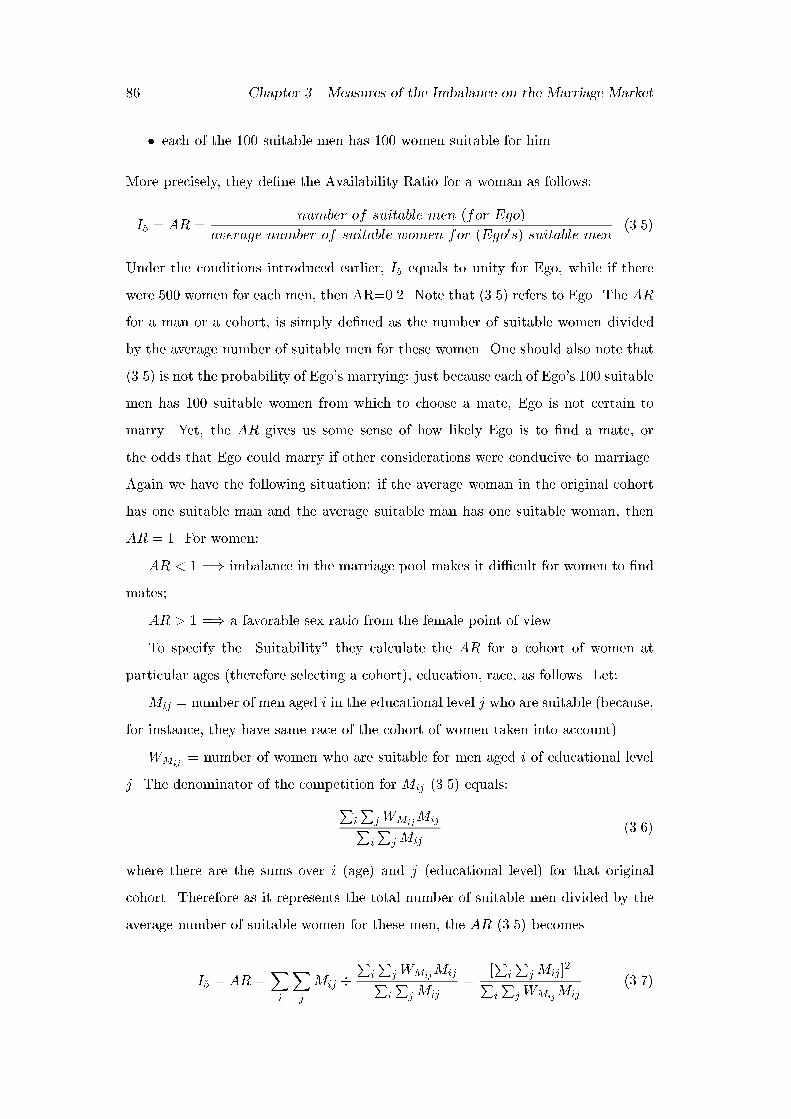
86 Chapter 3. Measures of the Imbalance on the Marriage Market
� each of the 100 suitable men has 100 women suitable for him.
More precisely, they de�ne the Availability Ratio for a woman as follows:
I5 = AR =number of suitable men (for Ego)
average number of suitable women for (Ego0s) suitable men(3.5)
Under the conditions introduced earlier, I5 equals to unity for Ego, while if there
were 500 women for each men, then AR=0.2. Note that (3.5) refers to Ego. The AR
for a man or a cohort, is simply de�ned as the number of suitable women divided
by the average number of suitable men for these women. One should also note that
(3.5) is not the probability of Ego's marrying: just because each of Ego's 100 suitable
men has 100 suitable women from which to choose a mate, Ego is not certain to
marry. Yet, the AR gives us some sense of how likely Ego is to �nd a mate, or
the odds that Ego could marry if other considerations were conducive to marriage.
Again we have the following situation: if the average woman in the original cohort
has one suitable man and the average suitable man has one suitable woman, then
AR = 1. For women:
AR < 1 =) imbalance in the marriage pool makes it di�cult for women to �nd
mates;
AR > 1 =) a favorable sex ratio from the female point of view.
To specify the \Suitability" they calculate the AR for a cohort of women at
particular ages (therefore selecting a cohort), education, race, as follows. Let:
Mij = number of men aged i in the educational level j who are suitable (because,
for instance, they have same race of the cohort of women taken into account)
WMij= number of women who are suitable for men aged i of educational level
j. The denominator of the competition for Mij (3.5) equals:
Pi
Pj WMij
MijPi
PjMij
(3.6)
where there are the sums over i (age) and j (educational level) for that original
cohort. Therefore as it represents the total number of suitable men divided by the
average number of suitable women for these men, the AR (3.5) becomes
I5 = AR =Xi
Xj
Mij �P
i
Pj WMij
MijPi
Pj Mij
=[P
i
Pj Mij]
2
Pi
PjWMij
Mij
(3.7)
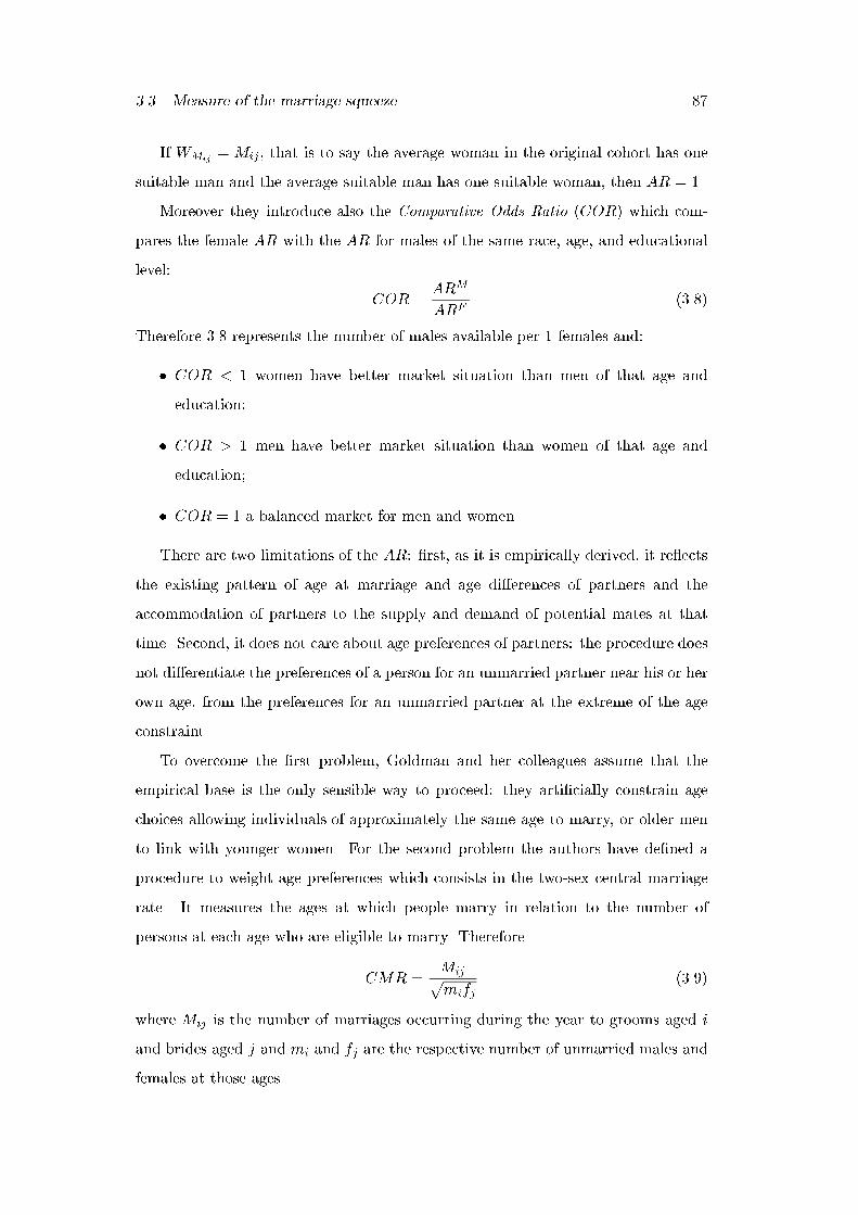
3.3. Measure of the marriage squeeze 87
If WMij=Mij , that is to say the average woman in the original cohort has one
suitable man and the average suitable man has one suitable woman, then AR = 1.
Moreover they introduce also the Comparative Odds Ratio (COR) which com-
pares the female AR with the AR for males of the same race, age, and educational
level:
COR =ARM
ARF(3.8)
Therefore 3.8 represents the number of males available per 1 females and:
� COR < 1 women have better market situation than men of that age and
education;
� COR > 1 men have better market situation than women of that age and
education;
� COR = 1 a balanced market for men and women.
There are two limitations of the AR: �rst, as it is empirically derived, it re ects
the existing pattern of age at marriage and age di�erences of partners and the
accommodation of partners to the supply and demand of potential mates at that
time. Second, it does not care about age preferences of partners: the procedure does
not di�erentiate the preferences of a person for an unmarried partner near his or her
own age, from the preferences for an unmarried partner at the extreme of the age
constraint.
To overcome the �rst problem, Goldman and her colleagues assume that the
empirical base is the only sensible way to proceed: they arti�cially constrain age
choices allowing individuals of approximately the same age to marry, or older men
to link with younger women. For the second problem the authors have de�ned a
procedure to weight age preferences which consists in the two-sex central marriage
rate. It measures the ages at which people marry in relation to the number of
persons at each age who are eligible to marry. Therefore
CMR =Mijpmifj
(3.9)
where Mij is the number of marriages occurring during the year to grooms aged i
and brides aged j and mi and fj are the respective number of unmarried males and
females at those ages.

88 Chapter 3. Measures of the Imbalance on the Marriage Market
The AR and COR have been applied to the Italian case (De Rose e Rufo,
1994[62]) in an analysis of the Italian population distributions by sex and mari-
tal status in various censuses (years 1936-1981). They obtain two major results, and
it is useful to summarise them brie y in view of our application. First, there is a
general disadvantage for women at most ages if one excludes the age-group15-19.
Second, the cohorts of women born during the two world wars and during the baby-
boom are in a better position on the marriage market than other women in the same
period. Moreover, under the assumptions that widowed and divorced people choose
their partners among their own, the position of these women in the marriage market
is even worse, because of the high sex mortality ratio at older ages. The analysis
of the COR ratio shows mainly the same results: a better position for women only
up to age 20, when the marriage market then becomes disadvantageous for them
(the number of single men available for single women decreases progressively) after
that age. Only for the 1981 census does there emerge a favourable situation for
women older than 40. The authors also note that, over time, the marriage market
conditions for single women at older ages improve as the rates, even if still negative,
become closer to 100. The 1981 situation is new, as we observe a rise of the COR
ratio at older ages (which means improving conditions for women at older ages): it
assumes the shape of a reversed J.
There are, however, some drawbacks to the measures we have just discussed.
First of all, the assumption that most partnerships are established within a given age
range or with a given age di�erence between partners does not provide the desired
exibility for measuring the marriage squeeze we are looking for. This is a key
aspect, especially when analyses are conducted over a longer time span. In fact, not
only the timing of marriage for men and women may change over time, but also the
age preferences of each partner may shift. Moreover, these measures exclude factors
other than age { and sometimes marital status { for de�ning the marriage market.
Obviously, many other social, economic, cultural, and personal factors should enter
into the de�nition of availability. Lastly, most existing ratios consider only cohorts in
their early twenties, thereby ignoring the question of availability for older unmarried
cohorts, which are becoming an increasingly larger percentage of the unmarried pool.
Schoen (1988[165]) observes, among others, that sex ratios only capture one-sex

3.3. Measure of the marriage squeeze 89
compositional e�ects. Even when re�ned, sex ratios combine changes in the age- and
sex-speci�c rates with one-sex compositional e�ects (marginal e�ects). To measure
the marriage squeeze, however, it would be necessary to measure the changes in age-
and sex-speci�c marriage rates which are produced by changes in the age and sex
composition of the population. Furthermore, such indices are not adequate for the
analysis of the Italian case. After a slight anticipation in age at marriage in the
early 1960s, marriage timing in Italy moved in the direction of higher ages at �rst
marriage and increasing variability at the regional level (De Sandre et al., 1997[64]).
Moreover the dispersion of the age distribution around the modal value is normally
higher in the male pattern than in the female one, so that �xing the age range would
exclude di�erent proportions of marriages.
3.3.2 Measures derived from the two-sex nuptiality tables
Several solutions to the so-called two-sex problem (that is, the reconciliation of male
and female rates) have been proposed in the literature. Two main families of models
can be envisaged: the axiomatic approach, which starts from a list of `axioms' have
been set as a requirement for an acceptable solution (Hoem 1969[102], Pollard 1975
[146], Schoen 1983[164]) and the behavioural approach, which starts from a set of
assumptions about the individual behaviour of candidates searching for a partner
(Henry 1972[96], Dagsvik 1998[58]). Some are based on the geometric, arithmetic,
or harmonic mean between the male and the female rates, others on the minimum
or maximum solution (they assume, for instance, the number of marriages to be the
minimum number obtained by multiplying the sex-speci�c rate by the corresponding
population). The main alternative approaches to the harmonic mean solution are
the iterative adjustment (McFarland, 1975[134]) and the panmitic circles approach
(Henry, 1972[96]). For a comparative analysis see Schoen (1988[166]) and Keilman
(1998[118]).
In 1983, Schoen [164] provides a formally precise de�nition of the marriage
squeeze. He considers the marriage squeeze as being closely associated with the
`two-sex problem' in formal demography.
`The two-sex problem is that a population's observed male and female marriage
(or fertility) rates cannot simultaneously be incorporated into demographic models,

90 Chapter 3. Measures of the Imbalance on the Marriage Market
or even be used to provide a consistent estimate of the number of marriages (or
births) a population might be expected to have in the following year' (Schoen, 1983,
p.62[164]).
To see why this is the case, let us consider marriage rates, bearing in mind the
obvious requirement that the number of males aged x marrying females aged y must
be the same as the number of females aged y marrying males aged x. When we
multiply the observed male rate for (x; y) marriages by the male population aged
x in some second population with a di�erent age-sex composition, we get a certain
number of (x; y) marriages. In general, however, that number will not be the same as
the number of (x; y) marriages produced by multiplying the �rst population's female
rate for (x; y) marriages by the number of females aged y in the second population.
Therefore, a change in age-sex composition forces a change in marriage rates, and
that is the kind of change which produces a marriage squeeze: we shall say that an
inconsistency between male and female marriage rates exists. In 1981, Schoen[162]
proposed for the discrete case to introduce an appropriate condition for consistency
between an observed and a model population, given by:
mW (xn; yn) +fW (xn; yn)| {z }
observed population
= mw(xn; yn) +fw(xn; yn)| {z }
model or second population
(3.10)
where the mW and fW represent observed male and female occurrence/exposure
rates of marriage between males aged x to x + n and females aged y to y + n and
the mw and fw represent the corresponding male and female rates in some second
or model population. In other terms:
mW (xn; yn) =M(xn; yn)mP (xn)
; fW (xn; yn) =M(xn; yn)fP (yn)
mw(xn; yn) =m(xn; yn)mL(xn)
; fw(xn; yn) =m(xn; yn)fL(yn)
where M(xn; yn) represents the number of marriages between males aged x to x+n
and females aged y to y+n in an observed population of males mP (xn) aged x; x+n
and of females fP (yn) aged y; y + n. Analogously, m(xn; yn) represents the number
of marriages between males aged x to x+ n and females aged y to y+ n in a model
population of males mL(xn) aged x; x+ n and of females fL(yn) aged y; y + n.
The consistency condition (3.10) is an harmonic mean consistency condition
(Schoen, 1981[162]) because it is equivalent to equating the observed population

3.3. Measure of the marriage squeeze 91
number of (xn; yn) marriages divided by the harmonic mean of the observed male
population aged x to x+n and the observed female population aged y to y+n with
the second population's number of (xn; yn) marriages divided by the harmonic mean
of its corresponding male and female populations:
M(xn; yn)mP (xn)
+M(xn; yn)fP (yn)
=m(xn; yn)mL(xn)
+m(xn; yn)fL(yn)
M(xn; yn)[fP (yn) +
mP (xn)]mP (xn)fP (yn)
=m(xn; yn)[
fL(yn) +mL(xn)]
fL(yn)mL(xn)
M(xn; yn)1
1mP (xn)
+1
fP (yn)
=m(xn; yn)
11
mL(xn)+
1fL(yn)
(3.11)
Schoen has shown that equation 3.10 reconciles the male and female rates and
he speci�ed and calculated two-sex life table models that re ect the complex inter-
actions of the observed marriage market.
In equation (3.10), the sum re ects the underlying reciprocal preference for mar-
riage between males aged x to x+n and females aged y to y+n: but these preferences
are in uenced by the age-sex composition of the population (the observed marriage
rates re ect this interaction).
Now, to provide a measure of the marriage squeeze, Schoen introduces the idea
of magnitude of marriage attraction between males and females in speci�ed age-sex
groups. Obviously, if the number of males and females in the two-sex age-groups is
the same, then there is no imbalance between the sexes and male and female rates
are equals. If the number of males and females is not the same, then the sex with
the larger population has a smaller rate, while the other sex has a larger rate. The
greater the imbalance between the number of males and the number of females, the
greater the di�erence between the male and the female rates. Thus the extent of
the imbalance is re ected in the di�erence between observed rates.
Let us take into account a rectangular population, where the number of people
is the same for every age: in this population there is no marriage squeeze, as the
population at risk for every age is the same for both sexes. As in every life table,
period and cohort experience are identical and in each birth cohort the number of
males who marry must be the same as the number of females who marry. Schoen
then adds the following assumptions:
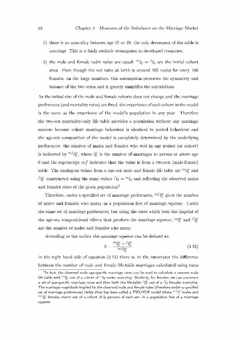
92 Chapter 3. Measures of the Imbalance on the Marriage Market
1) there is no mortality between age 15 to 49: the only decrement of the table is
marriage. This is a fairly realistic assumption in developed countries;
2) the male and female radix value are equal: ml0 = f l0 are the initial cohort
sizes. Even though the sex ratio at birth is around 105 males for every 100
females, on the large numbers, this assumption preserves the symmetry and
balance of the two sexes and it greatly simpli�es the calculations.
As the initial size of the male and female cohorts does not change and the marriage
preferences (and mortality rates) are �xed, the experience of each cohort in the model
is the same as the experience of the model's population in any year. Therefore
the two-sex nuptiality-only life table provides a population without any marriage
squeeze because cohort marriage behaviour is identical to period behaviour and
the age-sex composition of the model is completely determined by the underlying
preferences: the number of males and females who wed in any period (or cohort)
is indicated by mf lw0 , where lw0 is the number of marriages to person at above age
0 and the superscript mf indicates that the value is from a two-sex (male-female)
table. The analogous values from a one-sex male and female life table are mlw0 and
f lw0 constructed using the same values f l0 =ml0 and re ecting the observed males
and females rates of the given population3.
Therefore, under a speci�ed set of marriage preferences, mf lw0 gives the number
of males and females who marry in a population free of marriage squeeze. Under
the same set of marriage preferences, but using the rates which bear the imprint of
the age-sex compositional e�ects that produce the marriage squeeze, mlw0 and f lw0
are the number of males and females who marry.
According to the author the marriage squeeze can be de�ned as:
S =mlw0 � f lw0
mf lw0(3.12)
In the right hand side of equation (3.12) there is, in the numerator the di�erence
between the number of male and female life-table marriages calculated using rates
3In fact, the observed male age-speci�c marriage rates can be used to calculate a one-sex male
life table with mlw0 out of a cohort of ml0 males marrying. Similarly, for females, we can construct
a set of age-speci�c marriage rates and then built the life-table f lw0 out of a f l0 females marrying.
The marriage magnitude implied by the observed male and female rates (therefore under a speci�ed
set of marriage preferences) yields what has been called a TWONUP model where mf lw0 males andmf lw0 females marry out of a cohort of l0 persons of each sex, in a population free of a marriage
squeeze.
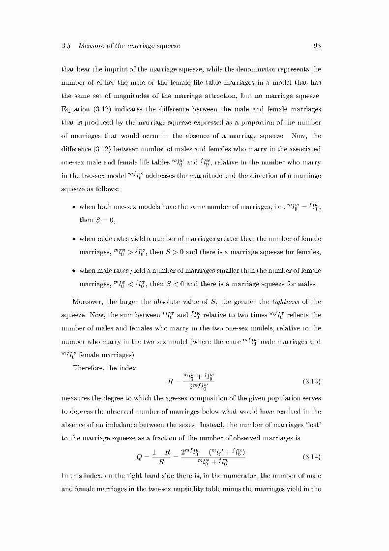
3.3. Measure of the marriage squeeze 93
that bear the imprint of the marriage squeeze, while the denominator represents the
number of either the male or the female life table marriages in a model that has
the same set of magnitudes of the marriage attraction, but no marriage squeeze.
Equation (3.12) indicates the di�erence between the male and female marriages
that is produced by the marriage squeeze expressed as a proportion of the number
of marriages that would occur in the absence of a marriage squeeze. Now, the
di�erence (3.12) between number of males and females who marry in the associated
one-sex male and female life tables mlw0 and f lw0 , relative to the number who marry
in the two-sex model mf lw0 addresses the magnitude and the direction of a marriage
squeeze as follows:
� when both one-sex models have the same number of marriages, i.e., mlw0 = f lw0 ,
then S = 0,
� when male rates yield a number of marriages greater than the number of female
marriages, mlw0 > f lw0 , then S > 0 and there is a marriage squeeze for females,
� when male rates yield a number of marriages smaller than the number of female
marriages, mlw0 < f lw0 , then S < 0 and there is a marriage squeeze for males.
Moreover, the larger the absolute value of S, the greater the tightness of the
squeeze. Now, the sum between mlw0 and f lw0 relative to two times mf lw0 re ects the
number of males and females who marry in the two one-sex models, relative to the
number who marry in the two-sex model (where there are mf lw0 male marriages and
mf lw0 female marriages).
Therefore, the index:
R =mlw0 + f lw02mf lw0
(3.13)
measures the degree to which the age-sex composition of the given population serves
to depress the observed number of marriages below what would have resulted in the
absence of an imbalance between the sexes. Instead, the number of marriages `lost'
to the marriage squeeze as a fraction of the number of observed marriages is
Q =1�R
R=
2mf lw0 � (mlw0 + f lw0 )mlw0 + f lw0
(3.14)
In this index, on the right hand side there is, in the numerator, the number of male
and female marriages in the two-sex nuptiality table minus the marriages yield in the

94 Chapter 3. Measures of the Imbalance on the Marriage Market
two one-sex life tables, while the denominator contains the number of marriages in
the one-sex models. Note that Q can never be negative, given that all three models
have the same radix value and have decrements only to marriage.
Now, the very usefulness of this model is due to the ease of application when
we come to a di�erent formulation of the previous indices S, R and Q, taking into
account that we can write (as a result of the piecewise constant rates) in each age
interval:
� = e�P
xnmW (xn;�) (3.15)
= e�
PynfW (�;yn) (3.16)
Where n is the width of the age-group, (�) indicates that marriages involving
persons of the other sex at all ages are included in the marriage rate and � and
can be though as the proportion of the male and the female life-table cohorts that
never marry (PNM). From the classical, or exponential life-table calculation we
also have that:
mlw0 = l0(1� �) (3.17)
f lw0 = l0(1� ) (3.18)
where l0 is the common radix. In the same way, also the two-sex nuptiality table
can follow the same line of reasoning:
mf lw0 = l0f1 � exp[�Xx
nmw(xn; �)]g = l0f1� exp[�Xy
nfw(�; yn)]g (3.19)
where the �nal equality is due to the fact that the male and female cohorts must
have the same number of marriages in the two-sex model.
Now, dividing the last equality in equation (3.19) by l0, rearranging and then
taking the logs, we have
Xx
nmw(xn; �) =Xy
nfw(�; yn) (3.20)
But the summations include all marriages, and then, we know from the basic
consistency condition (3.10) that:
Xx
nmW (xn; �) +Xy
nfW (�; yn) =Xx
nmw(xn; �) +Xy
nfw(�; yn) (3.21)

3.3. Measure of the marriage squeeze 95
Then, combining the last two equations (3.20) and (3.21) one gets:
Xx
nmw(xn; �) =Xy
nfw(�; yn) =1
2[Xx
nmW (xn; �) +Xy
nfW (�; yn)] (3.22)
and using (3.22) and (3.16) and (3.15):
mf l0 = l0(1�p �) (3.23)
Recalculating S, R and Q in (3.12), (3.13), (3.14), Schoen proposed the new version:
S = � �
1�p �
(3.24)
R =1� 1
2( + �)
1�p �
(3.25)
Q =12( + �)�
p �
1� 12( + �)
(3.26)
Now equations (3.24)(3.25)(3.26) are very useful because they show that, under
mild assumptions, we only need to know the two parameters and �, which are
simple functions of the sum of the observed age-speci�c male and female marriage
rates, to compute the Schoen's indices of imbalance on the marriage market. Thus
to �nd S, R, and Q is not necessary to calculate a whole life table or to know the full
arrays of mW (x; y) and fW (x; y) rates; the levels of the sums of the male and female
marriage rates su�ce. The size of those sums re ects the level of marriage, and the
di�erence between them re ects the severity of the marriage squeeze. Since in any
period equal numbers of males and females marry, the male and female rates share
in a sense the same numerators. If one sum exceeds the other, it is an indication
that the population in the denominators for that sex are smaller. Hence, there are
few of that sex relative to the number in the other sex, which thus �nd itself in a
marriage squeeze (Schoen, 1983[164]).
Before moving on, it is worth noting that Schoen's approach analyzes the dy-
namics of the interactions between the sexes in nuptiality.In his model marriage
preference depends only on age and sex, while other dimensions, as socio-economic
status, marital status and ethnicity are not considered.
96 Chapter 3. Measures of the Imbalance on the Marriage Market
3.3.3 Two new simple measures of the marriage squeeze
In this section, we take Schoen's reasoning as our starting point and describe two
measures that operate analogously to his S measure. The underlying idea is that
di�erences in the observed quantum of nuptiality between the two sexes indicate the
presence of a marriage squeeze.
Let us start from the observed Proportion Ever Marrying (PEM) for men
(PEMm) and for women (PEMf ), respectively. It should be stressed that the
quantities (3.15) and (3.16), introduced in the previous section express the Propor-
tion Never Married (PNM) for men and women respectively. In the same way, their
complementary measures are known as proportions ever marrying (PEM) and are
easily obtained as follows:
PEMm = 1� �
PEMf = 1�
Now, another very simple way to look for some evidence of the imbalance on the
marriage market could be obtained by taking into consideration the previous pro-
portions, in the following way:
I = Imbalance =PEMm � PEMf
PEMm + PEMf(3.27)
this index I expresses the di�erence in the proportion ever marrying in a nuptiality
table as a fraction of the sum of the proportions ever marrying in both sexes. This
index di�ers only very slightly from the one proposed by Schoen. It can however be
directly computed if one has access only to the proportion ever marrying. We can
see that the interpretation is quite similar to Schoen's index:
� when both one-sex populations have the same proportion ever marrying, then
I = 0, and there is no marriage squeeze;
� when male rates yield a proportion ever married higher than that for females,
then I > 0, and there is a marriage squeeze for females;
� when male rates yield a proportion ever married smaller than that for females,
then I < 0, and there is a marriage squeeze for males.

3.4. Trends over time in Italy 97
In addition to I, it could be useful to introduce here another even simpler and
alternative measure of the imbalance between the sexes. Often one has access only
to measures based on reduced events (Wunsch and Termote, 1978[190]) instead of
occurrence/exposure measures. As we also said in the previous chapter, reduced
events for marriage, are given by the number of marriages at each age divided by
the total age-speci�c population of that sex. The sum of age-speci�c �rst marriage
rates is the so-called Total First Marriage Rate TFMR. Starting from the sex-
speci�c measures TFMRm and TFMRf we can de�ne a similar index
Ifreq =TFMRm � TFMRf
TFMRm + TFMRf
(3.28)
The rationale behind the building of the indices I and Ifreq, is almost the same as
the one given by S (even though the denominators are still a�ected by the squeeze
experienced by the two populations), but in addition, they point to a further simpli�-
cation of the measure of the marriage squeeze. In particular, Ifreq has the advantage
of being solely based on the reduced events and, as a consequence, does not require
to pass through the building of the whole nuptiality tables, therefore providing an
easy tool of analysis of the unbalance between the sexes on marriage market. Some-
times occurrence/exposure rates for constructing nuptiality tables are not available.
In fact, that would require the distribution of the population by marital status,
which is not always available in non-censuses years, even in countries with fairly
good statistical records. On the other hand, the main disadvantage of our simple
indices is that they cannot be connected to measures of the theoretical impact of
the marriage squeeze such as Schoen's R and Q.
3.4 Trends over time in Italy
We now apply the above-mentioned measures of the marriage squeeze to Italian
nuptiality data from 1969 to 1995. Yet, before its application, we would like to
point out some other issues.
First, a two-sex nuptiality table is built starting from data which contain simul-
taneously the number of male and female marriages for each possible combination
of the spouses' ages. This means that we should have a double entry table where,
in each row the ages of the groom yn and in each column those of the bride xn ap-

98 Chapter 3. Measures of the Imbalance on the Marriage Market
pear. For each cell we could then calculate the marriage rate corresponding to that
exact combination of age of the groom and age of the bride: we would then have
all the partial distributions by age of the bride for each selected age of the groom
and viceversa. But, as most of the times data are available for each sex separately,
it is easier to build the two one-sex nuptiality tables (one for men and the other for
women). In this case, our information is limited to the knowledge of the marginal
distributions by age of the spouse, for each sex. As we see, this does not represent a
problem given that, the index of Schoen S, R, and Q, can be easily computed from
the two single sex life-tables and that also I and Ifreq can be built.
Second, in his work, Schoen started from occurrence/exposure rates of �rst mar-
riage. This are conditional �rst marriage rates built in the following way: at the
numerator they present the number of marriages occurring at that given age of the
groom (bride) and in the denominator there are the person-years lived in a year by
those males (females) in that particular age group without being married.
After building nuptiality tables for each sex at regional level and for the period
1969-1995 (see appendix, for a detailed description of the method followed to pass
from unconditional rates to marriage probabilities), the Schoen's indices described
earlier can be calculated. In fact, by applying the male and female rates to equations
(3.15) and (3.16):
� = PNMm = e�P
xmW (x;�) = e�
P49
x=15m�x
= PNMf = e�
PyfW (�;y)
= e�
P49
y=15f�y
one gets the proportion never married (PNM) for men and women respectively for
each year, and their complementary measures to unity, give the proportions ever
marrying (PEM).
In table 3.1 several indicators of Italian marriage intensity and marriage market
are reported. An increase in the proportion of never married people at age 50 for
both sexes (columns 3 and 6 respectively), but especially for men can be observed.
The probability that a women would never marry, given the 1969 preferences and
the years population composition was 18%, while this same probability reached the
value of 42% in 1995. Men, as well, experienced an increase in the proportion never
married from 17% in 1969 to 44% in 1995. Conversely, the proportion ever married

3.4. Trends over time in Italy 99
Table 3.1: Proportion ever married (PEM) and never married (Gamma and Beta)
at age 50 by sex and measures of the imbalance between the sexes: 1969-1995 -
ITALY
Alternative measures:marriages
TOT P.N.M. P.E.M. TOT P.N.M. P.E.M. Squeeze 'lost'YEAR ΣΣΣΣ
m ννννx ββββ 1 − β1 − β1 − β1 − β ΣΣΣΣ f ννννy γγγγ 1 − γ1 − γ1 − γ1 − γ S Q I Ifreq
1969 1.7531 0.1732 0.8268 1.7142 0.1801 0.8199 0.00835 0.000041 0.00417 0.006511970 1.8336 0.1598 0.8402 1.7889 0.1671 0.8329 0.00874 0.000049 0.00437 0.006911971 1.8629 0.1552 0.8448 1.8453 0.1580 0.8420 0.00327 0.000007 0.00164 0.002301972 1.8584 0.1559 0.8441 1.9023 0.1492 0.8508 -0.00790 0.000043 -0.00395 -0.007481973 1.8411 0.1586 0.8414 1.9168 0.1471 0.8529 -0.01364 0.000129 -0.00682 -0.012301974 1.7200 0.1791 0.8209 1.8076 0.1640 0.8360 -0.01813 0.000199 -0.00907 -0.015221975 1.5504 0.2122 0.7878 1.6206 0.1978 0.8022 -0.01810 0.000159 -0.00905 -0.013861976 1.4955 0.2241 0.7759 1.5212 0.2184 0.7816 -0.00731 0.000024 -0.00366 -0.005581977 1.4303 0.2392 0.7608 1.4532 0.2338 0.7662 -0.00710 0.000020 -0.00355 -0.005241978 1.3604 0.2565 0.7435 1.3755 0.2527 0.7473 -0.00515 0.000010 -0.00257 -0.003691979 1.2369 0.2903 0.7097 1.2331 0.2914 0.7086 0.00155 0.000001 0.00078 0.000871980 1.2155 0.2966 0.7034 1.1950 0.3027 0.6973 0.00877 0.000022 0.00439 0.005691981 1.1789 0.3076 0.6924 1.1456 0.3180 0.6820 0.01515 0.000063 0.00758 0.009691982 1.1394 0.3200 0.6800 1.0984 0.3334 0.6666 0.01989 0.000102 0.00995 0.012561983 1.0732 0.3419 0.6581 1.0310 0.3567 0.6433 0.02267 0.000120 0.01134 0.013991984 1.0407 0.3532 0.6468 0.9988 0.3683 0.6317 0.02366 0.000124 0.01183 0.014421985 1.0114 0.3637 0.6363 0.9726 0.3781 0.6219 0.02292 0.000111 0.01146 0.013801986 0.9851 0.3734 0.6266 0.9529 0.3856 0.6144 0.01969 0.000079 0.00985 0.011741987 1.0010 0.3675 0.6325 0.9779 0.3761 0.6239 0.01368 0.000040 0.00684 0.008201988 1.0216 0.3600 0.6400 1.0149 0.3624 0.6376 0.00376 0.000003 0.00188 0.002211989 1.0144 0.3626 0.6374 1.0150 0.3624 0.6376 -0.00030 0.000000 -0.00015 -0.000201990 0.9945 0.3699 0.6301 1.0038 0.3665 0.6335 -0.00541 0.000006 -0.00271 -0.003281991 0.9375 0.3916 0.6084 0.9583 0.3835 0.6165 -0.01314 0.000034 -0.00657 -0.007831992 0.9199 0.3985 0.6015 0.9555 0.3846 0.6154 -0.02286 0.000102 -0.01143 -0.013491993 0.8713 0.4184 0.5816 0.9090 0.4029 0.5971 -0.02623 0.000124 -0.01312 -0.015351994 0.8176 0.4415 0.5585 0.8569 0.4245 0.5755 -0.03000 0.000147 -0.01500 -0.017281995 0.8179 0.4414 0.5586 0.8749 0.4169 0.5831 -0.04281 0.000305 -0.02141 -0.02470
WOMENMEN Schoen's Indices:
Imbalance
(PEM in the table) decreased in the period that starts from 1969 to 1995. In
the same table the aggregate measure of the imbalance between the sexes are also
computed. According to Schoen (1983) the S index provides the proportion of the
di�erence between male and female marriages in the one-sex nuptiality tables as a
fraction of the number who marry in the two-sex model. As it can be also seen in
�gure 3.1, S and the alternative indices of imbalance I and Ifreq, show the same
pattern, although the former presents a stronger emphasis. All three measures are
negative, thus indicating a disadvantage on the marriage market for men, in the
period from 1971 to 1979, with the lowest levels reached in the years 1974-75, and
in the period after 1989. On the other hand, the indices show a marriage squeeze
for females for the years, 1969-1971 and for the years 1979-1989; the highest value
is reached in 1984. It seems, then, that the newly proposed indices describe the
existing imbalance on the marriage market rather well (table 3.1 and �gure 3.1).
The proportion of marriages `lost' because of the marriage squeeze (here we refer

100 Chapter 3. Measures of the Imbalance on the Marriage Market
Figure 3.1: Comparison between di�erent measures of the imbalance between the
sexes on the marriage market: 1969-1995 - ITALY
-0.05
-0.04
-0.03
-0.02
-0.01
0.00
0.01
0.02
0.03
1965 1970 1975 1980 1985 1990 1995 2000
years
Schoen's S
I
Ifreq
to Schoen's R) is at a maximum when the squeeze is tightest, regardless of its sign.
The highest loss is for the years 1974-75 and 1983-85. More recently, as the squeeze
has become tighter, the proportion of lost marriages has also been increasing (table
3.1).
The dynamics of the marriage squeeze are clearly challenging: how can we explain
such uctuations? As in US-based studies, we �rst look at the evolution of births.
By plotting the trend in the number of births and the measures of the squeeze
(S, I, Ifreq) together, we can get the idea of how variations in natality are echoed
in subsequent imbalances in the marriage market (�gure 3.2). The basic idea is that
women who were born during a period of growth in the number of births were more
likely to have trouble in �nding a proper match. In contrast, men born during a
phase of reduction in the number of births are more likely to �nd themselves in
a squeeze when searching for a partner. The time-scale of the abscissa at the top
exhibits a lag of 26 years with respect to the scale at the bottom, given that the
average age at marriage over the entire period and including both sexes is 25.7 years.
The latter �gure (at the bottom) is linked to the annual number of births, while
the former (the top) indicates the time scale for the index of imbalance. This can
provide us with a broad idea of the delayed e�ect of the variation in the birth cohorts
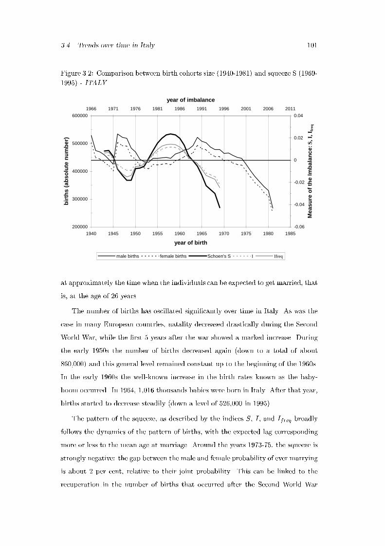
3.4. Trends over time in Italy 101
Figure 3.2: Comparison between birth cohorts size (1940-1981) and squeeze S (1969-
1995) - ITALY
200000
300000
400000
500000
600000
1940 1945 1950 1955 1960 1965 1970 1975 1980 1985
year of birth
bir
ths
(ab
solu
te n
um
ber
)
-0.06
-0.04
-0.02
0
0.02
0.04
1966 1971 1976 1981 1986 1991 1996 2001 2006 2011
year of imbalance
Mea
sure
of
the
Imb
alan
ce: S
, I, I
freq
male births female births Schoen's S I Ifreq
at approximately the time when the individuals can be expected to get married, that
is, at the age of 26 years.
The number of births has oscillated signi�cantly over time in Italy. As was the
case in many European countries, natality decreased drastically during the Second
World War, while the �rst 5 years after the war showed a marked increase. During
the early 1950s the number of births decreased again (down to a total of about
860,000) and this general level remained constant up to the beginning of the 1960s.
In the early 1960s the well-known increase in the birth rates known as the baby-
boom occurred. In 1964, 1,016 thousands babies were born in Italy. After that year,
births started to decrease steadily (down a level of 526,000 in 1995).
The pattern of the squeeze, as described by the indices S, I, and Ifreq broadly
follows the dynamics of the pattern of births, with the expected lag corresponding
more or less to the mean age at marriage. Around the years 1973-75, the squeeze is
strongly negative: the gap between the male and female probability of ever marrying
is about 2 per cent, relative to their joint probability. This can be linked to the
recuperation in the number of births that occurred after the Second World War
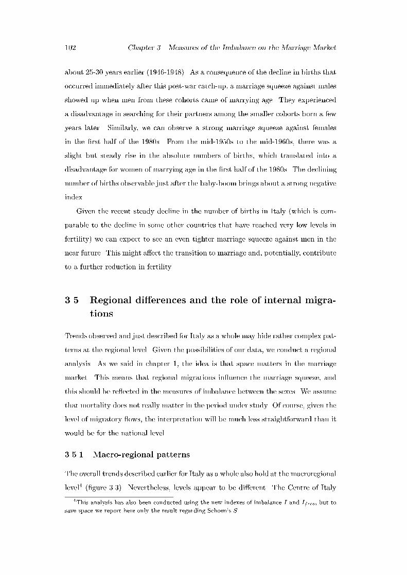
102 Chapter 3. Measures of the Imbalance on the Marriage Market
about 25-30 years earlier (1946-1948). As a consequence of the decline in births that
occurred immediately after this post-war catch-up, a marriage squeeze against males
showed up when men from these cohorts came of marrying age. They experienced
a disadvantage in searching for their partners among the smaller cohorts born a few
years later. Similarly, we can observe a strong marriage squeeze against females
in the �rst half of the 1980s. From the mid-1950s to the mid-1960s, there was a
slight but steady rise in the absolute numbers of births, which translated into a
disadvantage for women of marrying age in the �rst half of the 1980s. The declining
number of births observable just after the baby-boom brings about a strong negative
index.
Given the recent steady decline in the number of births in Italy (which is com-
parable to the decline in some other countries that have reached very low levels in
fertility) we can expect to see an even tighter marriage squeeze against men in the
near future. This might a�ect the transition to marriage and, potentially, contribute
to a further reduction in fertility.
3.5 Regional di�erences and the role of internal migra-
tions
Trends observed and just described for Italy as a whole may hide rather complex pat-
terns at the regional level. Given the possibilities of our data, we conduct a regional
analysis. As we said in chapter 1, the idea is that space matters in the marriage
market. This means that regional migrations in uence the marriage squeeze, and
this should be re ected in the measures of imbalance between the sexes. We assume
that mortality does not really matter in the period under study. Of course, given the
level of migratory ows, the interpretation will be much less straightforward than it
would be for the national level.
3.5.1 Macro-regional patterns
The overall trends described earlier for Italy as a whole also hold at the macroregional
level4 (�gure 3.3). Nevertheless, levels appear to be di�erent. The Centre of Italy
4This analysis has also been conducted using the new indexes of imbalance I and Ifreq, but to
save space we report here only the result regarding Schoen's S.
3.5. Regional di�erences and the role of internal migrations 103
Figure 3.3: Measure of the Squeeze in the macroregions: Italy, 1969-1995
-0.08
-0.06
-0.04
-0.02
0.00
0.02
0.04
0.06
0.08
1965 1970 1975 1980 1985 1990 1995 2000
years
Sq
uee
ze
NORTH
CENTRE
SOUTH
ITALY
has a di�erent behaviour for its almost always positive index of the squeeze: the
tightness of the squeeze in the Centre, which reaches the level +0.04 in the �rst half
of the 1980s (marriage squeeze for women), is the highest among those observed for
the other macroregions. Such a level of the squeeze (S = +0:04) means that the
male and female rates imply a gap between the male and female probability of ever
marrying, relative to their joint probability, of 4 percent (tables 3.2-3.3). The same
pattern holds true for southern regions, as well (where the highest level reached
in the middle of the 1980s is around 0.025), while northern regions experienced an
especially tight squeeze for men during the 1970s (maximum level of -0.03: negative
di�erence between male and female probability of ever marrying relative to their joint
of probability about 3 percent) and, recently, from the end of the 1980s onward.
On the whole, it seems that there was a marriage squeeze against men during
the 1970s and early 1990s in northern Italy, whereas in central and southern Italy
there was almost always a female disadvantage, which was especially high at the
beginning of the seventies and in the middle of the 1980s (�gure 3.3).
It is tempting to say that areas of high outmigration tended to have a squeeze for
women and viceversa for area of high immigration. With respect to this, however,
the Centre is rather heterogenous. One should then examine the evidence more
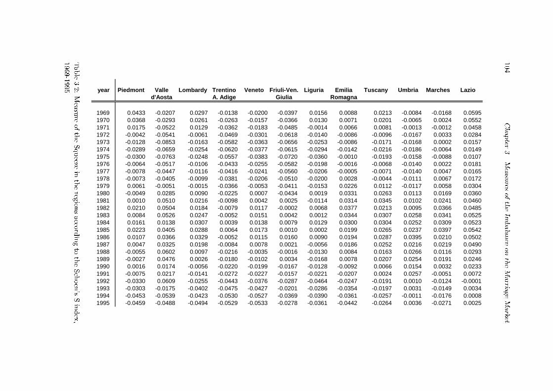
104
Chapter
3.Measures
oftheIm
balance
ontheMarria
geMarket
year Piedmont Valle Lombardy Trentino Veneto Friuli-Ven. Liguria Emilia Tuscany Umbria Marches Laziod'Aosta A. Adige Giulia Romagna
1969 0.0433 -0.0207 0.0297 -0.0138 -0.0200 -0.0397 0.0156 0.0088 0.0213 -0.0084 -0.0168 0.05951970 0.0368 -0.0293 0.0261 -0.0263 -0.0157 -0.0366 0.0130 0.0071 0.0201 -0.0065 0.0024 0.05521971 0.0175 -0.0522 0.0129 -0.0362 -0.0183 -0.0485 -0.0014 0.0066 0.0081 -0.0013 -0.0012 0.04581972 -0.0042 -0.0541 -0.0061 -0.0469 -0.0301 -0.0618 -0.0140 -0.0086 -0.0096 -0.0167 0.0033 0.02841973 -0.0128 -0.0853 -0.0163 -0.0582 -0.0363 -0.0656 -0.0253 -0.0086 -0.0171 -0.0168 0.0002 0.01571974 -0.0289 -0.0659 -0.0254 -0.0620 -0.0377 -0.0615 -0.0294 -0.0142 -0.0216 -0.0186 -0.0064 0.01491975 -0.0300 -0.0763 -0.0248 -0.0557 -0.0383 -0.0720 -0.0360 -0.0010 -0.0193 -0.0158 -0.0088 0.01071976 -0.0064 -0.0517 -0.0106 -0.0433 -0.0255 -0.0582 -0.0198 -0.0016 -0.0068 -0.0140 0.0022 0.01811977 -0.0078 -0.0447 -0.0116 -0.0416 -0.0241 -0.0560 -0.0206 -0.0005 -0.0071 -0.0140 0.0047 0.01651978 -0.0073 -0.0405 -0.0099 -0.0381 -0.0206 -0.0510 -0.0200 0.0028 -0.0044 -0.0111 0.0067 0.01721979 0.0061 -0.0051 -0.0015 -0.0366 -0.0053 -0.0411 -0.0153 0.0226 0.0112 -0.0117 0.0058 0.03041980 -0.0049 0.0285 0.0090 -0.0225 0.0007 -0.0434 0.0019 0.0331 0.0263 0.0113 0.0169 0.03601981 0.0010 0.0510 0.0216 -0.0098 0.0042 0.0025 -0.0114 0.0314 0.0345 0.0102 0.0241 0.04601982 0.0210 0.0504 0.0184 -0.0079 0.0117 -0.0002 0.0068 0.0377 0.0213 0.0095 0.0366 0.04851983 0.0084 0.0526 0.0247 -0.0052 0.0151 0.0042 0.0012 0.0344 0.0307 0.0258 0.0341 0.05251984 0.0161 0.0138 0.0307 0.0039 0.0138 0.0079 0.0129 0.0300 0.0304 0.0252 0.0309 0.05231985 0.0223 0.0405 0.0288 0.0064 0.0173 0.0010 0.0002 0.0199 0.0265 0.0237 0.0397 0.05421986 0.0107 0.0366 0.0329 -0.0052 0.0115 0.0160 0.0090 0.0194 0.0287 0.0395 0.0210 0.05021987 0.0047 0.0325 0.0198 -0.0084 0.0078 0.0021 -0.0056 0.0186 0.0252 0.0216 0.0219 0.04901988 -0.0055 0.0602 0.0097 -0.0216 -0.0035 -0.0016 -0.0130 0.0084 0.0163 0.0266 0.0116 0.02931989 -0.0027 0.0476 0.0026 -0.0180 -0.0102 0.0034 -0.0168 0.0078 0.0207 0.0254 0.0191 0.02461990 0.0016 0.0174 -0.0056 -0.0220 -0.0199 -0.0167 -0.0128 -0.0092 0.0066 0.0154 0.0032 0.02331991 -0.0075 0.0217 -0.0141 -0.0272 -0.0227 -0.0157 -0.0221 -0.0207 0.0024 0.0257 -0.0051 0.00721992 -0.0330 0.0609 -0.0255 -0.0443 -0.0376 -0.0287 -0.0464 -0.0247 -0.0191 0.0010 -0.0124 -0.00011993 -0.0303 -0.0175 -0.0402 -0.0475 -0.0427 -0.0201 -0.0286 -0.0354 -0.0197 0.0031 -0.0149 0.00341994 -0.0453 -0.0539 -0.0423 -0.0530 -0.0527 -0.0369 -0.0390 -0.0361 -0.0257 -0.0011 -0.0176 0.00081995 -0.0459 -0.0488 -0.0494 -0.0529 -0.0533 -0.0278 -0.0361 -0.0442 -0.0264 0.0036 -0.0271 0.0025
Table3.2:Measure
oftheSqueeze
inthereg
ionsacco
rdingto
theSchoen'sSindex,
1969-1995
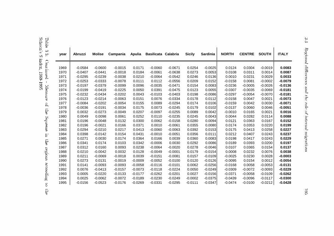
3.5.Regionaldi�eren
cesandtheroleofintern
almigratio
ns
105
year Abruzzi Molise Campania Apulia Basilicata Calabria Sicily Sardinia NORTH CENTRE SOUTH ITALY
1969 -0.0584 -0.0600 -0.0015 0.0171 -0.0060 -0.0671 0.0254 -0.0025 0.0124 0.0304 -0.0019 0.00831970 -0.0407 -0.0441 -0.0018 0.0184 -0.0061 -0.0638 0.0273 0.0053 0.0108 0.0311 0.0014 0.00871971 -0.0295 -0.0239 -0.0038 0.0210 -0.0064 -0.0542 0.0246 0.0136 0.0010 0.0231 0.0029 0.00331972 -0.0253 -0.0333 -0.0078 0.0111 0.0112 -0.0556 0.0209 0.0152 -0.0158 0.0081 -0.0002 -0.00791973 -0.0197 -0.0379 -0.0099 0.0096 -0.0035 -0.0471 0.0154 0.0083 -0.0236 -0.0005 -0.0026 -0.01361974 -0.0199 -0.0419 -0.0225 0.0050 0.0391 -0.0475 0.0123 0.0055 -0.0307 -0.0035 -0.0069 -0.01811975 -0.0232 -0.0434 -0.0202 0.0043 -0.0103 -0.0403 0.0198 -0.0086 -0.0297 -0.0054 -0.0070 -0.01811976 -0.0123 -0.0214 -0.0063 0.0151 0.0076 -0.0334 0.0178 0.0112 -0.0158 0.0047 0.0021 -0.00731977 -0.0084 -0.0202 -0.0054 0.0155 0.0089 -0.0294 0.0174 0.0106 -0.0159 0.0042 0.0030 -0.00711978 -0.0036 -0.0191 -0.0034 0.0175 0.0073 -0.0245 0.0179 0.0102 -0.0137 0.0060 0.0046 -0.00511979 0.0032 -0.0273 -0.0049 0.0207 -0.0097 -0.0255 0.0089 0.0042 -0.0010 0.0165 0.0021 0.00161980 0.0049 0.0098 0.0061 0.0252 0.0110 -0.0235 0.0245 0.0043 0.0044 0.0282 0.0114 0.00881981 0.0196 -0.0048 0.0132 0.0300 0.0062 -0.0158 0.0280 0.0094 0.0121 0.0363 0.0167 0.01521982 0.0196 -0.0021 0.0166 0.0371 0.0010 -0.0061 0.0355 0.0080 0.0174 0.0353 0.0220 0.01991983 0.0294 -0.0210 0.0217 0.0413 -0.0060 -0.0063 0.0392 0.0153 0.0175 0.0413 0.0258 0.02271984 0.0398 -0.0142 0.0154 0.0431 -0.0010 -0.0051 0.0356 0.0111 0.0212 0.0407 0.0243 0.02371985 0.0271 0.0030 0.0174 0.0364 0.0166 0.0039 0.0360 0.0083 0.0198 0.0417 0.0243 0.02291986 0.0341 0.0174 0.0103 0.0342 -0.0006 0.0030 0.0292 0.0086 0.0189 0.0393 0.0200 0.01971987 0.0312 0.0160 0.0093 0.0238 -0.0064 -0.0020 0.0278 -0.0046 0.0107 0.0365 0.0154 0.01371988 0.0210 -0.0042 0.0032 0.0128 -0.0049 -0.0001 0.0179 -0.0154 0.0008 0.0232 0.0076 0.00381989 0.0211 -0.0069 -0.0018 0.0039 -0.0151 -0.0081 0.0157 -0.0109 -0.0025 0.0230 0.0028 -0.00031990 0.0273 0.0131 -0.0019 -0.0009 -0.0052 -0.0100 0.0120 -0.0126 -0.0095 0.0154 0.0012 -0.00541991 0.0141 -0.0093 -0.0093 -0.0058 -0.0116 -0.0101 0.0062 -0.0256 -0.0168 0.0058 -0.0053 -0.01311992 0.0076 -0.0413 -0.0157 -0.0073 -0.0118 -0.0224 0.0050 -0.0249 -0.0309 -0.0072 -0.0093 -0.02291993 0.0005 -0.0220 -0.0133 -0.0177 -0.0262 -0.0201 0.0027 -0.0156 -0.0371 -0.0058 -0.0109 -0.02621994 0.0025 -0.0062 -0.0072 -0.0189 -0.0230 -0.0249 -0.0002 -0.0375 -0.0439 -0.0096 -0.0117 -0.03001995 -0.0156 -0.0523 -0.0176 -0.0269 -0.0331 -0.0295 -0.0111 -0.0347 -0.0474 -0.0100 -0.0212 -0.0428
Table
3.3:Contin
ued
-Measure
oftheSqueeze
inthereg
ionsacco
rdingto
the
Schoen'sSindex,1969-1995
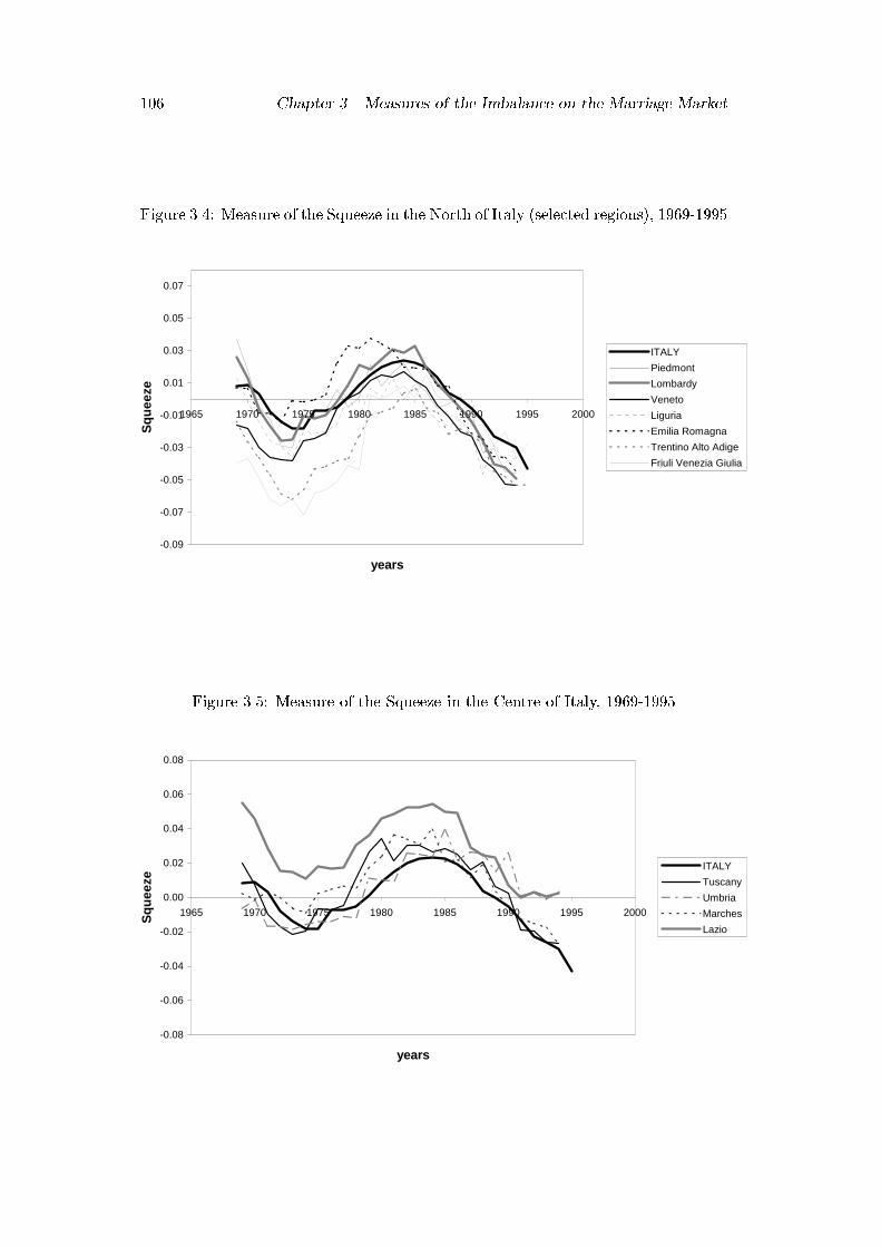
106 Chapter 3. Measures of the Imbalance on the Marriage Market
Figure 3.4: Measure of the Squeeze in the North of Italy (selected regions), 1969-1995
-0.09
-0.07
-0.05
-0.03
-0.01
0.01
0.03
0.05
0.07
1965 1970 1975 1980 1985 1990 1995 2000
years
Sq
uee
ze
ITALY
Piedmont
Lombardy
Veneto
Liguria
Emilia Romagna
Trentino Alto Adige
Friuli Venezia Giulia
Figure 3.5: Measure of the Squeeze in the Centre of Italy, 1969-1995
-0.08
-0.06
-0.04
-0.02
0.00
0.02
0.04
0.06
0.08
1965 1970 1975 1980 1985 1990 1995 2000
years
Sq
uee
ze
ITALY
Tuscany
Umbria
Marches
Lazio
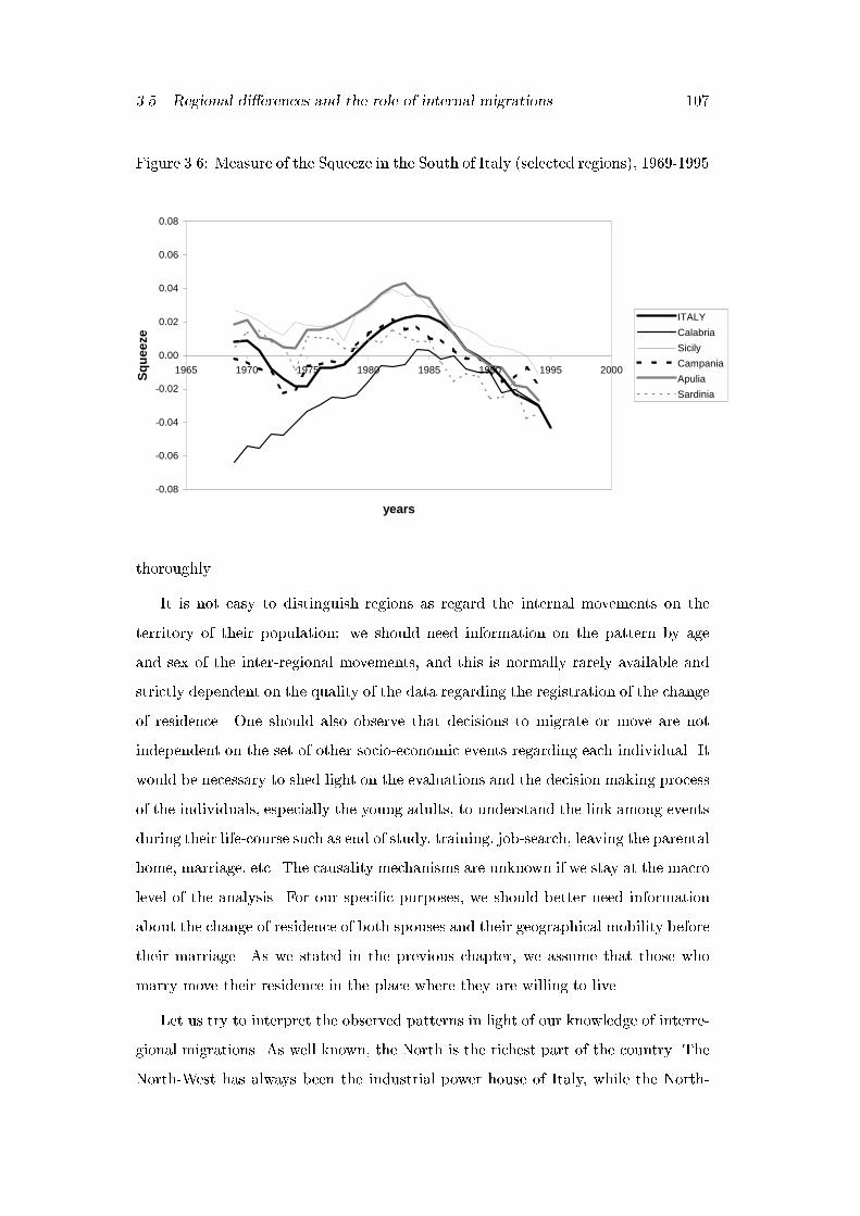
3.5. Regional di�erences and the role of internal migrations 107
Figure 3.6: Measure of the Squeeze in the South of Italy (selected regions), 1969-1995
-0.08
-0.06
-0.04
-0.02
0.00
0.02
0.04
0.06
0.08
1965 1970 1975 1980 1985 1990 1995 2000
years
Sq
uee
ze
ITALY
Calabria
Sicily
Campania
Apulia
Sardinia
thoroughly.
It is not easy to distinguish regions as regard the internal movements on the
territory of their population: we should need information on the pattern by age
and sex of the inter-regional movements, and this is normally rarely available and
strictly dependent on the quality of the data regarding the registration of the change
of residence. One should also observe that decisions to migrate or move are not
independent on the set of other socio-economic events regarding each individual. It
would be necessary to shed light on the evaluations and the decision making process
of the individuals, especially the young adults, to understand the link among events
during their life-course such as end of study, training, job-search, leaving the parental
home, marriage, etc. The causality mechanisms are unknown if we stay at the macro
level of the analysis. For our speci�c purposes, we should better need information
about the change of residence of both spouses and their geographical mobility before
their marriage. As we stated in the previous chapter, we assume that those who
marry move their residence in the place where they are willing to live.
Let us try to interpret the observed patterns in light of our knowledge of interre-
gional migrations. As well known, the North is the richest part of the country. The
North-West has always been the industrial power house of Italy, while the North-
108 Chapter 3. Measures of the Imbalance on the Marriage Market
East has seen a more recent industrial boom. The Centre is characterised by a new
model of dispersed and small- to medium-scale industrialisation. The South and the
Islands are a�ected by poverty in the interior regions and by economically stagnant
coastal towns and cities (Istat, 1998[107]). Throughout the post-war period, the
strongest ows have been from South-Islands to the North and internally within the
North (from North East to North West). Smaller ows have been targeted to the
central region of Lazio (mostly, to Rome) from the southern regions and central and
east coast provinces (Golini, 1974[87]).
From a very general point of view, migration rates at di�erent geographical
scales show that, at least for the comparison between 1955 and 1993, short-distance
(province-internal) migration was the most important, and it also declined the least.
The second-most important kind of movement was long-distance migration. Finally,
medium-distance migration between provinces was less important. By 1993 it had
fallen to half its 1955 level. Long-distance inter-regional, migration was a constant
factor over the period 1955-93. It was characterised by heavy out ows from the
South of Italy to the North before 1978 and by smaller out ows after that year
(Istat, 1998[107]).
The 1960s, the years of the `economic boom', saw a great deal of movements
across regional boundaries in Italy. Especially southern Italians moved towards the
economic triangle (Piedmont, Liguria and Lombardy) and towards northern Europe
(especially the Federal Republic of Germany and Switzerland). But the strongest
ow was directed towards the North of Italy. Between 1958 and 1963 more than
900,000 people left South Italy. Municipalities of the area of the industrialised trian-
gle (in the North West) experienced an increase of 69,000 new residents coming from
the South. In 1962, when an old fascist law against urbanisation was abrogated5,
this number jumped to 203,000 new unities and in 1963 kept an high level: 183,000
individuals (Ginsborg, 1989[77] ; Bonifazi et al.1999[28] ). South-to-north migration
losses are most marked for the young adult ages of labour force entry, between 15
and 29 years (Istat, 1998 [107]).
During the 1970s Italy underwent a trend that had started in the late 1960s,
5Intermunicipality migration rates had a marked peak in 1962, but this was due to considerable
adjustment of the registers after the 1961 Census to regularise urban registrations which has been
previously restricted by the fascist law on urbanisation [107].
3.5. Regional di�erences and the role of internal migrations 109
which is characterised by a reduction in both long- and short-distance geographical
mobility. This trend, which resulted from both economic and social factors, has been
called a `counter-urbanisation' process and it mainly refers to the transformations of
the ows that were earlier directed towards towns. The years 1973-1975 saw a sharp
decline in internal migrations, which was associated with the employment e�ect of
the �rst oil shock (Istat, 1998[107]). Of the Italian regions only Sicily exhibited
the opposite behaviour, as the dynamics to and from its towns increased in the
1970s (Micheli, 1988[135]). The 1980s were then characterised by a very low level of
inter-regional moment.
If we focus on the trend of the marriage market described by S, we notice the
existence, over the twenty-�ve years under study, of a pattern of imbalance between
the sexes which can be explained by the internal movement of the Italian population.
At the regional level, we observe that the general pattern regarding the divi-
sions holds, although some regions exhibit a certain degree of deviations therefrom.
Among the central regions, for example, Lazio has particularly striking (�gure 3.5)6.
It has an extremely high and positive level of S over the entire period, which means
that women are subject to a marriage squeeze in general. Thus, there is no simple
connection between in- and out-migration and the direction of the squeeze. The
South, in contrast, is characterised by two strong, distinct patterns. On the one
hand, Sicily and parts of Apulia exhibit a constant, positive level of the imbalance
to the disadvantage of women, whereas Calabria, on the other hand, shows a degree
of marriage squeeze that increases from a very low level up to a zero, which was
reached in the mid-1980s, only to fall again (�gure 3.6 and table 3.3). Northern re-
gions have very high S values, which approach one another when negative. Veneto,
Liguria, and Piedmont, in particular, are areas where the squeeze against men is
particularly tight (�gure 3.4 and table 3.2).
These apparently contradictory results stimulated us to perform a deeper analysis
of two neighbouring regions of the South with di�erent marriage market dynamics:
Calabria and Sicily.
6In this region the presence of Rome, Italy's capital, is a relevant factor.

110 Chapter 3. Measures of the Imbalance on the Marriage Market
3.5.2 Evaluating some regional di�erences: Calabria and Sicily
The need to �nd an explanation of the regional patterns of imbalances observed in
the marriage market requires to go deeper into a �ner level of analysis. As it has
been observed from other scholars (Cantisani, Dalla Zuanna 1996[39]), long term
analyses of the nuptiality patterns need to take into account the marriage market
features as embedded in a system composed also of other demographic processes,
like births and migrations. An attempt of evaluation can be presented if we consider
the pattern of the squeeze associated to some selected regions.
Our reasoning is here based on the assumption that mortality di�erentials did
not play a striking role in comparison to that assumed by birth uctuations and
migration di�erentials. It could be argued that the period under study, from 1955
to 1995, has been characterised by increasing gains in life expectancy, especially to
women's advantage, and that the pattern by cause of death greatly shifted its pro�le
by age and sex. Yet, there is no reason to believe that this could have been di�erent
at the regional level when comparing, for instance, Calabria and Sicily. Most of the
di�erences in the local marriage markets are here mainly attributed to birth size
di�erences and to the role of the migratory movements.
In this section we focus on a dynamic comparison of the marriage squeeze in
two regions: Sicily and Calabria (table 3.4 and �gure 3.7). In Sicily there prevails
a disadvantage for women in the marriage market (Ifreq always positive), while in
Calabria it is men who are in a worse position over time (Ifreq is almost always
negative).
The two neighbouring (and mostly outmigration) regions share very similar fer-
tility trends (Santini, 1997[106]). Since 1940 the birth pattern is characterised by
a drop during the Second World War period, which was followed by a \catch-up
process" in the second half of the 1940s, and then a slight decline over time. In con-
trast, the two regions have a very di�erent history of migratory movements, which
is highly di�erentiated between men and women (table 3.5). First of all, it must
be noted that there are no data available on the in ow and out ow on migratory
movements by marital status7. It should also be stressed that data regarding place
7Nor is the population distribution by marital status available at the regional level, except for
in censuses years. Estimates are available for Italy as a whole for the years 1952-1981 (Castiglioni,
1989[43]).

3.5. Regional di�erences and the role of internal migrations 111
Table 3.4: Summary of the main indicators for Calabria and Sicily, 1969-1995
calendaryear Difference Difference
Men Women Ifreq Men Women in ave. Men Women Ifreq Men Women in ave.ages ages
1969 912.3 1014.3 -0.0529 27.01 22.93 4.08 1035.3 992.0 0.0214 27.03 23.00 4.031970 934.9 1037.6 -0.0521 27.03 22.92 4.11 1069.9 1020.0 0.0239 27.03 22.91 4.121971 971.1 1065.8 -0.0465 27.22 23.12 4.1 1079.4 1033.8 0.0216 26.98 22.92 4.061972 973.4 1072.5 -0.0484 27.01 23.13 3.88 1084.6 1045.7 0.0182 26.99 23.14 3.851973 979.3 1062.6 -0.0408 27.24 23.06 4.18 1086.9 1058.4 0.0133 26.94 23.06 3.881974 902.9 972.0 -0.0369 26.95 22.90 4.05 1038.5 1018.0 0.0100 26.90 22.97 3.931975 904.2 961.9 -0.0309 26.99 22.78 4.21 978.6 949.5 0.0151 26.75 22.97 3.781976 876.6 920.5 -0.0245 27.08 22.95 4.13 955.6 930.4 0.0134 26.87 23.08 3.791977 857.7 894.3 -0.0209 27.06 22.93 4.13 935.2 911.4 0.0129 26.85 23.09 3.761978 835.7 864.4 -0.0169 27.07 22.90 4.17 911.3 888.0 0.0130 26.83 23.08 3.751979 745.9 770.3 -0.0161 27.14 23.10 4.04 858.6 847.9 0.0062 26.79 23.24 3.551980 792.9 817.3 -0.0151 26.93 22.83 4.1 887.8 856.3 0.0181 26.72 22.98 3.741981 770.5 785.7 -0.0098 27.08 22.89 4.19 864.0 830.1 0.0200 26.68 22.99 3.691982 762.7 767.8 -0.0033 27.09 22.93 4.16 855.2 813.6 0.0249 26.75 23.03 3.721983 731.6 736.4 -0.0033 27.12 22.97 4.15 821.9 779.6 0.0264 26.82 23.15 3.671984 739.3 743.3 -0.0027 27.15 23.08 4.07 811.9 774.1 0.0238 26.89 23.30 3.591985 728.7 724.5 0.0029 27.37 23.26 4.11 798.0 761.0 0.0238 26.96 23.36 3.61986 721.9 718.6 0.0023 27.49 23.37 4.12 801.3 770.8 0.0193 27.06 23.49 3.571987 729.5 730.8 -0.0009 27.57 23.54 4.03 801.7 772.6 0.0185 27.15 23.59 3.561988 730.7 730.2 0.0003 27.60 23.54 4.06 832.7 812.5 0.0123 27.23 23.79 3.441989 717.1 724.0 -0.0048 27.74 23.81 3.93 825.6 808.0 0.0108 27.33 23.92 3.411990 713.5 722.0 -0.0059 27.92 23.97 3.95 816.3 803.2 0.0081 27.41 24.10 3.311991 694.0 702.4 -0.0060 28.08 24.26 3.82 760.1 754.1 0.0040 27.45 24.12 3.331992 658.7 676.5 -0.0133 28.22 24.45 3.77 765.4 760.3 0.0033 27.62 24.35 3.271993 630.4 645.3 -0.0117 28.33 24.47 3.86 713.3 710.9 0.0016 27.78 24.49 3.291994 602.4 619.9 -0.0143 28.68 24.85 3.83 661.4 661.6 -0.0001 28.06 24.70 3.361995 604.5 625.5 -0.0171 28.85 25.18 3.67 643.4 651.9 -0.0066 28.31 24.96 3.35
CALABRIA SICILY
TFMR Mean Age TFMR Mean Age
Figure 3.7: Imbalance in the marriage market measure between Calabria and Sicily,
1969-1995
Imbalance Ifreq for selected regions
-0.06
-0.04
-0.02
0.00
0.02
0.04
0.06
1969 1971 1973 1975 1977 1979 1981 1983 1985 1987 1989 1991 1993 1995
year
Ifre
q
Sicily
Calabry
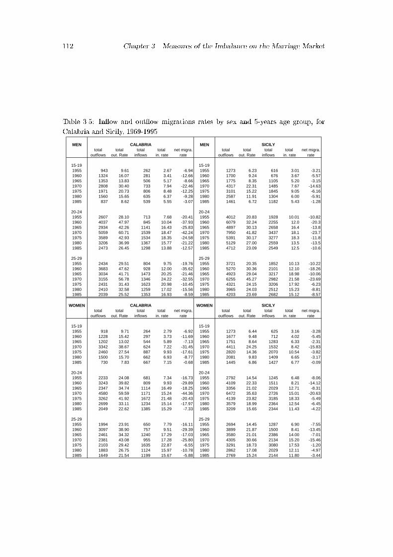
112 Chapter 3. Measures of the Imbalance on the Marriage Market
Table 3.5: In ow and out ow migrations rates by sex and 5-years age group, for
Calabria and Sicily, 1969-1995
MEN MENtotal total total total net migra. total total total total net migra.
outflows out. Rate inflows in. rate rate outflows out. Rate inflows in. rate rate
15-19 15-191955 943 9.61 262 2.67 -6.94 1955 1273 6.23 616 3.01 -3.211960 1324 16.07 281 3.41 -12.66 1960 1700 9.24 676 3.67 -5.571965 1353 13.83 506 5.17 -8.66 1965 1775 8.35 1105 5.20 -3.151970 2808 30.40 733 7.94 -22.46 1970 4317 22.31 1485 7.67 -14.631975 1971 20.73 806 8.48 -12.25 1975 3101 15.22 1845 9.05 -6.161980 1560 15.65 635 6.37 -9.28 1980 2587 11.91 1304 6.00 -5.911985 837 8.62 539 5.55 -3.07 1985 1461 6.72 1182 5.43 -1.28
20-24 20-241955 2607 28.10 713 7.68 -20.41 1955 4012 20.83 1928 10.01 -10.821960 4037 47.97 845 10.04 -37.93 1960 6079 32.24 2255 12.0 -20.31965 2934 42.26 1141 16.43 -25.83 1965 4897 30.13 2658 16.4 -13.81970 5059 60.71 1539 18.47 -42.24 1970 7950 41.82 3437 18.1 -23.71975 3589 42.93 1534 18.35 -24.58 1975 5391 30.17 3277 18.3 -11.81980 3206 36.99 1367 15.77 -21.22 1980 5129 27.00 2559 13.5 -13.51985 2473 26.45 1298 13.88 -12.57 1985 4712 23.09 2549 12.5 -10.6
25-29 25-291955 2434 29.51 804 9.75 -19.76 1955 3721 20.35 1852 10.13 -10.221960 3683 47.62 928 12.00 -35.62 1960 5270 30.36 2101 12.10 -18.261965 3034 41.71 1473 20.25 -21.46 1965 4923 29.04 3217 18.98 -10.061970 3155 56.78 1346 24.22 -32.55 1970 6255 45.27 2982 21.58 -23.691975 2431 31.43 1623 20.98 -10.45 1975 4321 24.15 3206 17.92 -6.231980 2410 32.58 1259 17.02 -15.56 1980 3965 24.03 2512 15.23 -8.811985 2039 25.52 1353 16.93 -8.59 1985 4203 23.69 2682 15.12 -8.57
WOMEN WOMENtotal total total total net migra. total total total total net migra.
outflows out. Rate inflows in. rate rate outflows out. Rate inflows in. rate rate
15-19 15-191955 918 9.71 264 2.79 -6.92 1955 1273 6.44 625 3.16 -3.281960 1228 15.42 297 3.73 -11.69 1960 1677 9.48 712 4.02 -5.451965 1202 13.02 544 5.89 -7.13 1965 1751 8.64 1283 6.33 -2.311970 3342 38.67 624 7.22 -31.45 1970 4411 24.25 1532 8.42 -15.831975 2460 27.54 887 9.93 -17.61 1975 2820 14.36 2070 10.54 -3.821980 1500 15.70 662 6.93 -8.77 1980 2081 9.83 1409 6.65 -3.171985 730 7.83 667 7.15 -0.68 1985 1445 6.86 1427 6.77 -0.09
20-24 20-241955 2233 24.08 681 7.34 -16.73 1955 2792 14.54 1245 6.48 -8.061960 3243 39.82 809 9.93 -29.89 1960 4109 22.33 1511 8.21 -14.121965 2347 34.74 1114 16.49 -18.25 1965 3356 21.02 2029 12.71 -8.311970 4580 59.59 1171 15.24 -44.36 1970 6472 35.63 2726 15.01 -20.631975 3262 41.92 1672 21.48 -20.43 1975 4139 23.82 3185 18.33 -5.491980 2699 33.11 1234 15.14 -17.97 1980 3579 18.99 2364 12.54 -6.451985 2049 22.62 1385 15.29 -7.33 1985 3209 15.65 2344 11.43 -4.22
25-29 25-291955 1994 23.91 650 7.79 -16.11 1955 2694 14.45 1287 6.90 -7.551960 3097 38.90 757 9.51 -29.39 1960 3899 21.87 1500 8.41 -13.451965 2461 34.32 1240 17.29 -17.03 1965 3580 21.01 2386 14.00 -7.011970 2381 43.08 955 17.28 -25.80 1970 4305 30.66 2134 15.20 -15.461975 2103 29.42 1635 22.87 -6.55 1975 3291 18.73 3080 17.53 -1.201980 1883 26.75 1124 15.97 -10.78 1980 2862 17.08 2029 12.11 -4.971985 1649 21.54 1199 15.67 -5.88 1985 2769 15.24 2144 11.80 -3.44
SICILYCALABRIA
CALABRIA SICILY
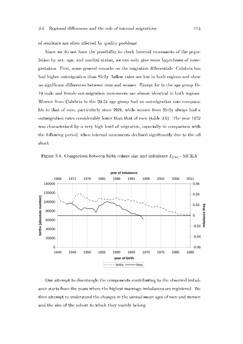
3.5. Regional di�erences and the role of internal migrations 113
of residence are often a�ected by quality problems.
Since we do not have the possibility to check internal movements of the popu-
lation by sex, age, and marital status, we can only give some hypotheses of inter-
pretation. First, some general remarks on the migration di�erentials. Calabria has
had higher outmigration than Sicily. In ow rates are low in both regions and show
no signi�cant di�erences between men and women. Except for in the age group 15-
19 male and female out-migration movements are almost identical in both regions.
Women from Calabria in the 20-24 age group had an outmigration rate compara-
ble to that of men, particularly since 1970, while women from Sicily always had a
outmigration rates considerably lower than that of men (table 3.5). The year 1972
was characterised by a very high level of migration, especially in comparison with
the following period, when internal movements declined signi�cantly due to the oil
shock.
Figure 3.8: Comparison between birth cohort size and imbalance Ifreq - SICILY
0
20000
40000
60000
80000
100000
120000
140000
1940 1945 1950 1955 1960 1965 1970 1975 1980 1985
year of birth
bir
ths
(ab
solu
te n
um
ber
)
-0.06
-0.04
-0.02
0
0.02
0.04
0.06
1966 1971 1976 1981 1986 1991 1996 2001 2006 2011
year of imbalance
imb
alan
ce If
req
births Ifreq
Our attempt to disentangle the components contributing to the observed imbal-
ance starts from the years where the highest marriage imbalances are registered. We
then attempt to understand the changes in the annual mean ages of men and women
and the size of the cohort to which they mainly belong.
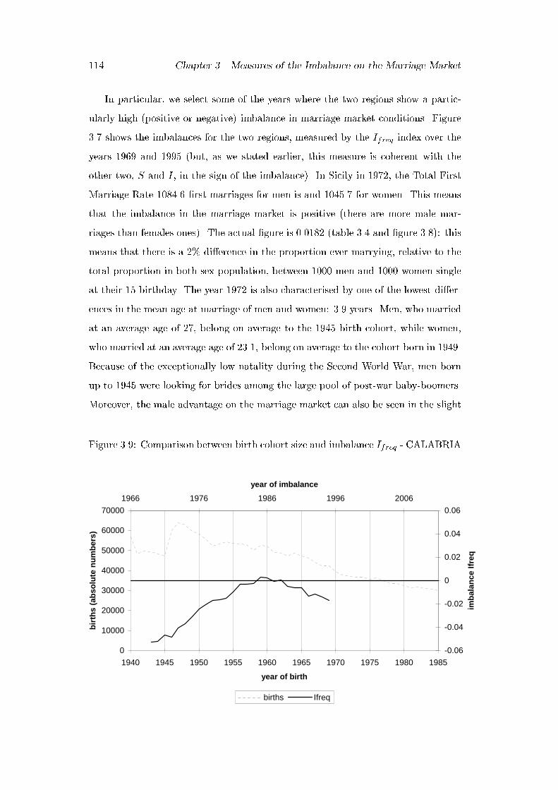
114 Chapter 3. Measures of the Imbalance on the Marriage Market
In particular, we select some of the years where the two regions show a partic-
ularly high (positive or negative) imbalance in marriage market conditions. Figure
3.7 shows the imbalances for the two regions, measured by the Ifreq index over the
years 1969 and 1995 (but, as we stated earlier, this measure is coherent with the
other two, S and I, in the sign of the imbalance). In Sicily in 1972, the Total First
Marriage Rate 1084.6 �rst marriages for men is and 1045.7 for women. This means
that the imbalance in the marriage market is positive (there are more male mar-
riages than females ones). The actual �gure is 0.0182 (table 3.4 and �gure 3.8): this
means that there is a 2% di�erence in the proportion ever marrying, relative to the
total proportion in both sex population, between 1000 men and 1000 women single
at their 15 birthday. The year 1972 is also characterised by one of the lowest di�er-
ences in the mean age at marriage of men and women: 3.9 years. Men, who married
at an average age of 27, belong on average to the 1945 birth cohort, while women,
who married at an average age of 23.1, belong on average to the cohort born in 1949.
Because of the exceptionally low natality during the Second World War, men born
up to 1945 were looking for brides among the large pool of post-war baby-boomers.
Moreover, the male advantage on the marriage market can also be seen in the slight
Figure 3.9: Comparison between birth cohort size and imbalance Ifreq - CALABRIA
0
10000
20000
30000
40000
50000
60000
70000
1940 1945 1950 1955 1960 1965 1970 1975 1980 1985
year of birth
bir
ths
(ab
solu
te n
um
ber
s)
-0.06
-0.04
-0.02
0
0.02
0.04
0.06
1966 1976 1986 1996 2006
year of imbalance
imb
alan
ce If
req
births Ifreq
3.5. Regional di�erences and the role of internal migrations 115
shifts in period-speci�c age at marriage. When compared to previous years, the
male mean age in 1972 is in a phase of slight decrease while that of women is rising.
Furthermore, the positive situation for men was accentuated by the fact that women
did not migrate with the same intensity as men did. The low mobility of women in
Sicily put them in a very disadvantageous position with respect to marriage. In a
nutshell, in 1972 Sicily the male advantage in the marriage market is essentially the
outcome of the di�erential sizes of cohorts.
In comparison, it is striking to see that the sign of the squeeze in Calabria is
always to the disadvantage of men. And this although Calabria shared the same
declining birth pattern as Sicily (and Italy as a whole) during the war and the same
rise in birth rates afterwards. We assume then that di�erential migratory movements
between sexes have played a key role (table 3.5). It is worth noting that the net
migration rates for the women in Calabria after 1970 are higher than they are for
men in the age groups 15-19 and 20-24. Of course, we do not know the marital
status of these young migrant women, but since they left at such young ages, we can
assume that the majority of them were unmarried at the time of their move (or that
they moved to marry a partner they had already met).The pool of eligible women
was thus diminished. This improved the chance for young women to get married
while it caused a marriage squeeze for the men. The high level of migration of young
women can be assumed to be the main reason for men's disadvantage in Calabria in
1972 and surrounding years.
In 1979 there was still imbalance in Sicily to the disadvantage of women, although
an equilibrium had almost been reached. Here the key to interpreting the situation
is the slight postponement in the age at marriage of women born around 1955-56
(who had a mean age at marriage of 23.2 years) and of men born around 1952 (who
had a mean age at marriage of 26.8 years), together with the slight decline in births
that occurred in the early 1950s and the ensuing rise in the second half of that
decade. In 1979, in fact, the di�erence between the mean ages at marriage, just 3.6
years, is again one of the lowest observed for this region8.
8It should also be noted that it is not necessarily a noticeable reverse in timing that takes place
to compensate for an imbalance in the cohort sizes among which men and women choose their
partners. It is often just a slight increase in the mean age of those in the unfavourable position as
well as a slight decline in the age of those in the more favourable position that can compensate for
the outcome (Schoen, 1983 [164]).
116 Chapter 3. Measures of the Imbalance on the Marriage Market
To arrive at an adequate interpretation of the imbalance in Sicily in 1983 one
needs to include some further factors. The imbalance in favour of men is fairly
high in that year (Ifreq = 0:0264), and the mean age at marriage is around 27 for
men and 23 for the women, with a precise di�erence of 3.7 years. The natality
component does not contribute very much to clarifying the situation. The 27 year-
old grooms belong on average to the cohort born in 1956 and the 23 year-old brides
were born on average in 1959-60. In the late 1950s there was a slight increase in
births in Sicily, which may have been partly responsible for a female disadvantage.
Furthermore, analysing the age pattern of nuptiality rates for some selected years,
we notice that in Sicily (and, with less emphasis, also in other southern regions)
there was a sudden increase in the rate of marriage for 18-year-olds (�gure 3.10).
The introduction of a law concerning the family reformation in terms of nuptiality
can help in the understanding of the phenomenon. According to the new law, the
minimum age at marriage was set at 18 for both men and women9. In Sicily, where
the timing of marriage had been particularly early for women, the introduction of
this law turned out to have an abrupt delaying e�ect on the behaviour of potential
brides. The proportion of those who marry at 18 years is extraordinarily high
starting with the cohort of women born in 1957 (�gure 3.10). This age e�ect can be
largely attributed to the institutional change. The postponement of entry into �rst
union for this birth cohort further increased the disadvantage of women, who were
already in an unfavourable position due to their low mobility.
Lastly, Calabria as depicted in 1983 observes a more balanced marriage market,
as the Total First Marriage Rates for men and women have almost the same level:
731.6 �rst marriages for men and 736.4 for women. The mean age is about 27 years
for men and 23 for women, with a di�erence of slightly over 4 years. Here the cohorts
involved are mainly men born in 1955-56 and women born in 1960. It should also be
noted that the left-skewed bell-shaped pattern for Calabria in 1983 is characterised
by a fork between ages 18 and 20 for women in the 1960 cohort and between age 18
and 26 years for men in the 1950 and 1955 cohort (�gure 3.10). Here again we can
imagine that the reduction in the level of out-migration, which also meant a greater
9Some exceptions allowing people to marry at younger ages were and are still allowed but only
through a judge's ruling.
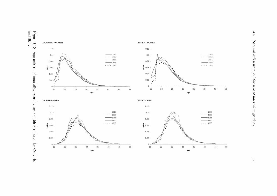
3.5.Regionaldi�eren
cesandtheroleofintern
almigratio
ns
117
CALABRIA - WOMEN SICILY - WOMEN
CALABRIA - MEN SICILY - MEN
0
0.02
0.04
0.06
0.08
0.1
0.12
15 20 25 30 35 40 45 50
age
rate
s
1945
1950
1955
1960
1965
0
0.02
0.04
0.06
0.08
0.1
0.12
15 20 25 30 35 40 45 50
age
rate
s
1945
1950
1955
1960
1965
0
0.02
0.04
0.06
0.08
0.1
0.12
15 20 25 30 35 40 45 50
age
rate
s
1945
1950
1955
1960
1965
0
0.02
0.04
0.06
0.08
0.1
0.12
15 20 25 30 35 40 45 50
age
rate
s
1945
1950
1955
1960
1965
Figure
3.10:Agepattern
ofnuptia
lityrates
bysex
andbirth
cohorts,
forCalabria
andSicily
118 Chapter 3. Measures of the Imbalance on the Marriage Market
degree of similarity between the sexes than in Sicily, together with the changes in
the timing of marriage (a slight decline in mean age for men and a slight rise in the
mean age for women) ended up balancing the marriage market.
From the comparative analysis of Calabria and Sicily, we notice that the e�ect
of uctuations in natality and of migratory movements (together with the sex di�er-
entials in migrations) have been highly intertwined in shaping the marital chances
at the regional level. We also have some evidence that the legal change concerning
the minimum age at marriage played a relevant role.
3.6 Summary
In this chapter, we studied the marriage market from a dynamic perspective. The
Italian case is particularly interesting due to the strong uctuations of the post-war
period, from baby boom to baby bust. The measures proposed in the literature
arising from two-sex demography, in particular Schoen's index, together with other
simple alternatives such as our measures based on reduced events, allowed us to
trace the dynamics of the marriage squeeze and to compare it to the evolution of
births at the national level.
Our main �nding is that there is an imbalance on the Italian marriage mar-
ket that stems from signi�cant variations in the number of births. Some cohorts
of women �nd themselves in a marriage squeeze (basically the 1980s) while other
cohorts of men, especially those born after the post-war rise in births or after the
baby-boom, face this same unfavourable situation. The squeeze was particularly
strong for women in the Centre and the South of Italy in the early 1970s and the
1980s, while the same was true for men, especially in the North, during the 1970s
and since the beginning of the 1990s.
In addition, we showed that migration, especially di�erential migration by sex,
had a crucial role in determining the extent of the marriage squeeze at a regional
level. The cases of Calabria and Sicily showed that migratory patterns matter. Some
evidence was also found for an in uence of the institutional setting, namely the legal
norms determining the minimum age at marriage.
This reasoning does not take into account possible shifts in preferences across
3.6. Summary 119
cohorts, as regard qualitative aspects of the partner choice, such as those regarding
his/her employment, his/her social status, his/her educational level or other macro
factors such as the unemployment rate at the local level, the condition of the housing
market, etc. It should also be noted that, in general, the measures used lack of
considerations about the e�ects of the squeeze to some crucial ages, where the impact
of the squeeze might be decisive even for future catch up behaviour. Therefore there
is a need for more in-depth analysis aiming at evaluating age and sex-speci�c impact
of the structural constraints arising from an unsteady growth of the population.
However, our �ndings are particularly important in light of current developments
in the number of births in Italy (and, most likely, in other European countries as
well). They show that, if there is no in uence of migration, a marriage squeeze
against men can be expected for the coming decades. Immigration may change this,
of course, depending on the sex composition of the migrants. In any case, it seems
that a marriage squeeze resulting from a decline in births might itself be the cause
of a subsequent decline in births, especially in those countries where marriage is still
crucial for reproduction.

120 Chapter 3. Measures of the Imbalance on the Marriage Market
Chapter 4
The marriage market and the
transition to marriage
4.1 Introduction
In the previous chapter we stressed the relevance of the compositional constraints
observed on the Italian marriage market, because they can be considered as factors
that might potentially a�ect the process of mate selections. In this chapter, our
purpose is to evaluate the impact of macro variables regarding the availability of
eligible partners in shaping the process of transition to �rst marriage in a micro
perspective for men and women. Many theories presented in chapter 1 highlighted
the role played by the constraints on the marriage market in shaping the chances
of marriage at the individual level, particularly if we think about some speci�c and
small pools.
In this chapter the process of transition to �rst marriage in Italy, resulting from
the behaviour of the individuals included in the 1998 Multipurpose Household Survey
is studied together with some other transitions typical of the early adulthood and
particularly relevant for the previous one (entry into �rst job). Moreover, individual
life-courses have been linked to the macro (aggregate) measures of the marriage
squeeze introduced in chapter 3. Both measures proposed in this work for the �rst
time (see chapter 3) and the one introduced by Schoen (1983[164]) are used as
indicators of the marriage squeeze observed in Italy.
The analysis will be conducted dividing the survey sample in sub-groups, by sex
and, mainly, 10-years birth cohorts. To highlight the territorial di�erences and their
trends over time, it turns out useful, to adopt a broader classi�cation of cohorts of
121
122 Chapter 4. The marriage market and the transition to marriage
analysis (<= 1935, 1936 � 65, >= 1966). Age is the duration variable.
The e�ect of the marriage squeeze (measured in the previous chapter through S
obtained from the nuptiality table, I, obtained by dividing the di�erence between
men and women in the proportion ever married, by their sum, and Ifreq, computed
from �rst marriage tables based on rates of the second kind, also known as reduced
events or frequencies) is introduced as a time-dependent covariate both for the region
of birth and for that of residence at the interview.
The present chapter is structured as follows. The next section deals with the
data and their quality problems used in this part of our work. Section 3 is dedicated
to the description of the techniques used in the chapter: mainly nonparametric
models of event history for the analysis of age at �rst marriage and semiparametric
and parametric models for the evaluation of the impact of macro variables of the
squeeze on the transition to �rst marriage. Therefore, the analyses presented in this
chapter can be distinguished into two parts. The �rst (section 4) aims at describing
the transition to �rst marriage, by applying nonparametric methods by sex, birth
cohort, territorial level (section 4.1). The second part (section 5) is devoted to
the search and the evaluation of an e�ect of the marriage squeeze on the Italian
marriage market by using models with di�erent assumptions about the pattern of the
time dependence of the rate. Moreover, nonnested parametric models incorporating
the e�ect of alternative indexes of the squeeze are compared. Section 6 aims at
broadening the framework of the transition to �rst marriage: section 6.1 takes shortly
into account the transition to the �rst job and section 6.2 aims at evaluating the
role of the marriage market, controlling for birth cohort, region of birth, level of
attained education and entry into the labour market. The last section is devoted
to the summary of the outcomes. The appendix to this chapter is dedicated to the
explanation of the models and their estimates.
4.2 Data and quality problems
This part of the work is based on the analysis of the data from the Italian Household
Survey, carried out by the National Institute of Statistics (ISTAT), in 1998, on a na-
tional representative sample of about 59,000 belonging to 24,000 Italian households.
This survey belongs to an integrated system of sample social surveys that has been

4.2. Data and quality problems 123
Table 4.1: Sex and marital status distribution at the Survey (age >= 15 years),
ITALY
MARITAL STATUS MEN WOMEN
Married 14875 14875Separated de facto 195 264Separated de jure 214 294Divorced 150 262Widowed 578 2794TOTAL 16012 18489
Single (censored) 7564 6331TOTAL 23576 24820
arranged on a new framework, since 19931.
The special topic of the 1998 survey is `Households, Social Subjects and Condi-
tions of the Infancy'. Retrospective information on several topics and dimensions of
the individual life-courses have been collected from all members of the household.
We focus our attention on individuals older than 15 years at the time of the
survey and on age at �rst marriage, that represents our dependent variable under
study. Table 4.1 contains the description of �rst marriages by marital status of the
sample, as observed in the sample at the time of the survey (June 1998). Our total
sample is therefore composed by 48,396 individuals older than 15 years and the total
number of events is of 34,501 �rst marriages. Since only �rst marriages are taken
into account, there has been the need to rebuild the information about that marriage
both for those currently married (not necessarily at their �rst marriage2) and for
those who were married (currently widowed, separated or divorced). Consensual
1On average each of those surveys deals with 24,000 households which correspond to about
70,000 individuals and collects information on about 800 variables. One annual survey on living
conditions and �ve thematic surveys, rotating in a time slot of �ve years, constitute an integrated
system covering the most important social topics: daily life, health, leisure time and culture, family
and social subjects, citizen's safety and time use and tourism.2Some quality problems are those regarding the lapse recall for the date of �rst marriage es-
pecially for men, currently married and in couple, that are not directly asked about their �rst
marriage (which could be di�erent from the current one). In such a case their current wife is asked
to remember whether and when he married �rst.

124 Chapter 4. The marriage market and the transition to marriage
unions3 and same sex unions are left apart4.
Though the survey design is retrospective, some problems have been encoun-
tered in drawing the life-courses of the individuals and, as a consequence, in the
application of our event history analysis. To perform our analysis, the requirement
would be a complete collection of information of the educational, working and mar-
ital career. First of all, in order to evaluate the role of the marriage market in
the individual's marriage opportunities, we would need to follow his/her territorial
movements among regions. The survey provides us with the information about the
residence at the survey time time (post) and at birth (ante), but it lacks any other
information between the two. A question regarding the change of residence during
the �rst job searching process has been included in the questionnaire. Unfortunately,
such information has not been registered and we, therefore, cannot have a vague idea
of the role played by the intermediate (between that of birth and that of current
residence) market.
However, also for those who never worked before, it would be sensible to know
which was their residence when, say, they were approximately at the beginning of
their marriageable ages (because, for example, they could have followed their fam-
ily's movements). For instance, given that a section of the survey deals with `his/her
parents' education and work' when the interviewed was approximately 15 years old,
it would have been wise to include also a question about the place of residence at
that time. A question of this kind has been included in a survey conducted in France
and it turned out to be a bit more successful than the place of birth in identifying
the marriage market of the couples (Bozon, 1987[34]). Another problem is due to the
incoherence among the possible answers regarding the educational status and the
educational attainment: the former includes also the possibility of being enrolled in
vocational training courses which is, on the contrary, excluded from the latter set of
answers. Moreover, we would like to know exactly when people ended their studies,
also in case they abandoned them, earlier than expected, without attaining the �nal
3The 1998 household survey showed that 14,875 couples, out of 15,203, are married couples:
consensual unions at the time of the survey represent only 2.2% of all couples. As well known, in
comparison to other western countries, premarital cohabitation in Italy still represents a marginal
phenomenon. In particular in 1998, around 6% of all Italian couples experienced a premarital
cohabitation.4We do not have any kind of information about these couples.
4.2. Data and quality problems 125
degree. In fact, any additional year spent in the educational system is expected
to increase the human capital of the individual. Educational attainment underesti-
mates the involvement in the educational system of the individuals, especially in a
country like Italy, where the permanence in it is prolonged and when it plays a very
important role in the process of family formation in comparison to other European
countries (Blossfeld, 1995[69], Pinnelli and De Rose, 1995[145]).
Another weakness of the survey pertains to the collection of the timing of some
peculiar event. Although the problems related to the de�nition of premarital co-
habitation and of consensual union, to study these emergent phenomena it should
be necessary to know the date of entry into and exit from each consensual unions.
Probably, measurement errors arise from the questions regarding the duration of
the consensual union as well as of the past cohabitation experience. In both cases,
the question does not lead to the identi�cation of the timing of such events nor to
their multiple experiences during the individual life-courses. Information regarding
the length of the life span spent in a union is meaningless if we do not know the
starting time of such a union, especially in the case of past experiences that did not
result into a formal union5. It would be useful to collect information regarding the
history of the unions independently from the marital status of the individuals. If the
aim is to distinguish between di�erent paths followed by the individuals belonging
to a population, it should be sensible to go in depth in their `biography' as concern
the history of their unions. However, consensual unions, still relatively few in Italy,
mainly act as an intermediate variable in the process of transition to �rst marriage.
Next analyses will not distinguish between direct marriage or a �rst marriage with
previous cohabitation.
5In this case we cannot even subtract the duration of that experience from the date of marriage,
as could be done in the case of a premarital cohabitation.

126 Chapter 4. The marriage market and the transition to marriage
4.3 Techniques of analysis
Over the last 20 years, event history data collection6 and analysis have become in-
creasingly spread among social scientists. There has been common agreement in the
recognition that the substantive process under study is based on few characteristics
which can be summed up in the following way: the units of analysis (not necessarily
individuals, but also, for instance, organisations, societies) move from one discrete
status to another (because an event occurs); this change occurs at any point in
time; time-constant and/or time-dependent factors in uence the events (Coleman,
1990[53]).
Moreover, a great theoretical emphasis has been given to the importance of the
mode of explanation of the behaviour of social systems that entails examining pro-
cesses internal to the system, involving its components parts, or units at a level
below that of the system (Coleman, 1990[53]). Thus explaining macro-changes re-
quires to consider changes in the individual level behaviour, and therefore, the link
between macro and micro changes (Giele and Elder, 1998[75]).
The present study uses this theoretical approach in analysing marriage be-
haviour. As we stated in the �rst chapter, we should consider marriages as the
results of the matching opportunities and of the preferences, expectations and norms
regarding the assortative mating (Kalmijn, 1998[113]). Opportunities of marriage
are here identi�ed by the macro demographic features of the marriage market for
each calendar year and region, as it is shown in greater detail later. Event history
analysis regarding the transition to �rst marriage will be conducted in two main
steps: the �rst deals with the description of the behaviour by birth cohort and sex
and the second with models including the e�ects of some covariates as well as some
time-period e�ects.
In this �rst part, a descriptive analysis of the processes characterised by single
non-renewable events along a continuous time axis is presented. In particular, we
refer to the set of techniques of description of a process with a single state of origin
6It consists in the collection of the timing of events occurred along the life course of the units. An
event-oriented observation design records all the changes in qualitative variables and their timing.
In this way one can get the most complete data regarding changes in the qualitative variables
that may occur at any point in time. E.H. data can be collected longitudinally mainly through a
retrospective survey and/or a panel survey. For a description of the advantages and disadvantages
of these data collection see Blossfeld and Rohwer, 1995[24].
4.3. Techniques of analysis 127
and a single state of destination (Blossfeld and Rowher, 1995[24]).
The well-known life table approach represents the classical method yielding non-
parametric estimates of the survivor function, and transition rates, for durations
given in a set of episodes. The life table methods require to group durations accord-
ing to some intervals on the time axis, but this cause some drawbacks that should be
considered. First, results depend more or less on arbitrarily de�ned time intervals
and, second, the method should be applied if there is a relatively large number of
episodes, that makes estimates conditional for each interval reliable.
An alternative method for nonparametric estimation of survivor functions and its
derivatives is the Kaplan-Meier (1958[115]) or product-limit method. This approach
has been suggested by several researchers7 but it is mainly attributed to Kaplan
and Meier (1958[115]). Kaplan and Meier showed that its estimators are maximum
likelihood estimators and then it emerged as the standard for survivor function
estimations. A basic characteristic of the product-limit estimator is that it does not
require any distribution assumption and, as we said, it di�ers from the life-table
method because it does not require any arbitrarily de�ned division of time into
intervals. Instead, the product-limit method is based on the calculation of a risk set
at every point in time where at least one event occurs, so that the researcher does not
intervene in choosing time intervals of analysis, but, on the contrary, intervals derive
directly from the observed durations (Blossfeld and Rower, 1995[24]). Product-limit
estimation method is here introduced as a �rst descriptive tool for the transition to
�rst marriage in Italy controlling for some basic characteristics.
Appendix to this chapter, is dedicated to a brief description of the main features
of the method which will then be applied in our analysis. For further explanations
of the method see Collett (1997[55]), Rohwer and P�otter (1998[150]), Blossfeld and
Rohwer (1995[24]), Yamaguchi (1991[191]), Tuma and Hannan (1984[179]), Allison
(1984[2]). The analysis has been performed by using TDA.
4.3.1 Linking macro and micro data
The bulk of our analyses attempts to directly ascertain the e�ect of the supply of
spousal alternatives on the transition into �rst marriage in Italy. According to the
7Namboodiiri and Suchindran (1987[140]) stated that the Product-Limit approach to the esti-
mation of the survival function was proposed by B�ohmer in 1912.
128 Chapter 4. The marriage market and the transition to marriage
indexes presented in chapter 3, we argue that the pattern of the marriage squeeze
may have hampered or eased the experience of our event under study (marriage) in
a di�erent way between women and men. Our aim is therefore to link the macro
level of analysis, expressing the conditions on the marriage market, and the micro
level of analysis represented by the life-course of the individuals. We should recall
that variables at the macro level are measures of the marriage squeezes built cross-
sectionally using nuptiality tables for each calendar year, while variables at the micro
level represent individual life-courses data taken from the 1998 survey.
In �gure 4.1 we report the information coming from both sources having on the
x-axis the calendar years, and on the y-axis the age of the individuals (cohorts). Let
us say that cross-sectionally, for each calendar year 1969-1995 and for each region we
have two nuptiality tables (for both sexes) which describe the marriage pattern for
ages 15-49 (see chapter 2). As described in chapter 3, for each year three synthetic
indicators of the squeeze have been built (S or I or Ifreq) starting from the male and
the female �rst-marriage tables and, somehow, summarising their total age-pattern.
In particular S was the Schoen index expressing the di�erence between the male
and female marriages that is produced by the squeeze expressed as a proportion of
the number of marriages that would occur in the absence of a marriage squeeze. I
has been proposed in this research to simplify the previous index as it is expressed
by the di�erence over the sum of the male and female proportion ever married from
the nuptiality table and lastly Ifreq represents the imbalance in the marriage market
measured from the total nuptiality rate obtained summing up over ages the second
type rates. Thus we have 20 (one for each region) indicators of the squeeze (of each
type: S or I or Ifreq) relatively to each of the calendar year 1969-95. This macro
level represents the features of the marriage market (positive values of S; I; and
Ifreq denote an imbalance against women, while negative values indicate a squeeze
against men) and it is then linked to the individuals' experiences, corresponding to
the micro level. The survey conducted in June 1998 contains information collected
retrospectively on marriage for every individual belonging to the household included
in the sample. In particular, for the individuals we look at: their age at the time of
the survey, birth cohort, region of birth, region of current residence, attained level of
education, �rst job, date of their �rst marriage. It should be stressed that in order

4.3. Techniques of analysis 129
to link the two levels of analysis (macro and micro) we need to look at the birth
cohorts who start their path, their life-courses since the very beginning at age 15.
Individual life-courses resulting to be left-censored in 1969 (all the area above the
diagonal in �gure 4.1) cannot be included simply because for them we are not able
to measure the macro variable occurring at every age of their life: for instance, we
have the measure of the squeeze occurring, say, at age 20 in 1969 for the cohort born
in 1949, but we do not know which was the existing imbalance before that age for
the same birth cohort. We need to follow only the individual life-courses that start
from age 15 on.
Figure 4.1 describes the common part between the two sources: it includes the
years 1969-1995, ages 15-41 and birth cohorts 1954-1980. It is important to note that
the right censoring does not correspond to the survey time, but it is instead arranged
on the 31st December 1995. Thus individual data were all censored at the end of
1995 because we did not have access to the macro variables after 1995. Moreover,
in this �rst part of our analysis, in order to have a su�cient amount of information
and to evaluate the impact of the compositional constraints (the squeeze) on the
most completed cohorts, we decided to focus our analysis on birth cohorts 1955-64;
aged 31-41 at the time of the survey (grey area).
The assumptions which we introduce in the analysis of the imbalances between
the sexes at the territorial level are the following. For each individual there can be
at least two major pools within which to look for a partner:
� the region of origin
� the region of residence at the time of the survey
Of course, people might move at every stage in their life, widening the horizon of
their marriage market, and might even return to their starting point (their region
of residence might, after a long time spent traveling around, eventually coincide
with their region of birth, for instance) and, therefore, we would loose the complete
history of the individual. As we already said, the 1998 household survey collected
the information regarding the destination region in case of migratory movements
due to �rst job search reasons, but this information then was lost.
It is worthwhile to highlight that our macrolevel analyses provide us with time-
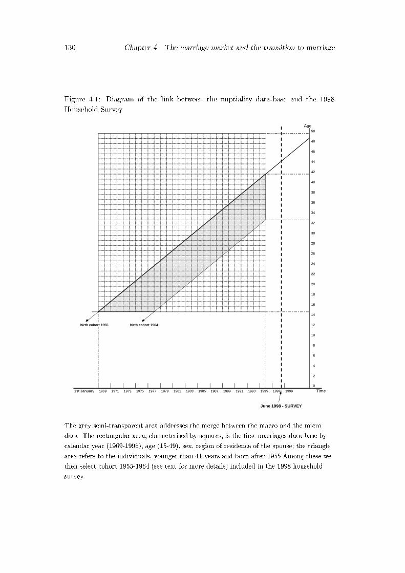
130 Chapter 4. The marriage market and the transition to marriage
Figure 4.1: Diagram of the link between the nuptiality data-base and the 1998
Household Survey
Age50
48
46
44
42
40
38
36
34
32
30
28
26
24
22
20
18
16
14
birth cohort 1955 birth cohort 1964 12
10
8
6
4
2
0
1st January 1969 1971 1973 1975 1977 1979 1981 1983 1985 1987 1989 1991 1993 1995 1997 1999 Time
June 1998 - SURVEY
The grey semi-transparent area addresses the merge between the macro and the micro
data. The rectangular area, characterised by squares, is the �rst-marriages data-base by
calendar year (1969-1996), age (15-49), sex, region of residence of the spouse; the triangle
area refers to the individuals, younger than 41 years and born after 1955.Among these we
then select cohort 1955-1964 (see text for more details) included in the 1998 household
survey.
4.3. Techniques of analysis 131
varying indicators of the squeeze8. To entail the link between the aggregate and
the individual level it is necessary that the individual episodes are split accordingly.
With this procedure we can divide each episode (or spell, or duration time before
the occurrence of the event under study or before the interview) referred to as a unit
of analysis, into sub-episodes known as splits, where the imbalance measure of the
marriage market is allowed to vary. In our case, each episode starts at age 15 and
ends either at �rst marriage or at the end of the year 1995. Our macro variables,
S,I, and Ifreq represent our covariates changing their values only at the beginning
of a calendar year and yearly constant9.
In such a way, the measure of the imbalance plays a role in each region of birth
(as well as in each region of current residence) and calendar year. Consequently, each
individual's age will be a�ected during his/her life-course by a time-varying squeeze.
The result of the split consists in having divided the time axis into time-periods in
correspondence of the 1st of January of each year and to assume that the transition
rates are constant in each of these intervals but can change between them.
In particular, the episode splitting procedure is a method for handling time-
varying covariates and therefore to include their e�ect on the causal explanation of
the model. The procedure requires that at all points in time where at least one of
the explanatory variables changes its value, the time axis is split into sub-episodes,
called splits of the episode. In each split the explanatory variables assume di�erent
values; all the episode splits have the same state of origin and state of destination,
which is equal to the origin state of the original episode and are therefore considered
as censored; the last split assumes a destination state equal to destination state in
the original episode.
8Our imbalance on the marriage market is, as we said, a synthetic measure meaning that is
annual measure but it varies at regional level and for every calendar year.9In particular, the episode splitting procedure can be brie y described as follows. The original
episode is split into sub-episodes and each of them constitutes a new record containing information
about the origin state of the original episode, the values of all the covariates at the beginning of
the sub-episodes, the starting and ending times of the sub-episode, information indicating whether
the sub-episodes end with the destination state of the original episode or they are censored. All
the episodes, except the last one, are regarded as right censored. Only the last episode is given the
same destination state as the original episode.
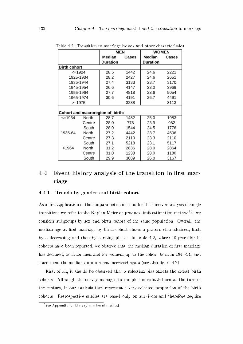
132 Chapter 4. The marriage market and the transition to marriage
Table 4.2: Transition to marriage by sex and other characteristics
Median Cases Median CasesDuration Duration
Birth cohort28.5 1442 24.6 222128.2 2427 24.6 265127.4 3133 23.7 317026.6 4147 23.0 396927.7 4818 23.6 505430.6 4191 26.7 4491
3288 3113
Cohort and macroregion of birth:<=1934 North 28.7 1482 25.0 1983
Centre 28.0 778 23.9 982South 28.0 1544 24.5 1776
1935-64 North 27.2 4442 23.7 4506Centre 27.3 2110 23.3 2110South 27.1 5218 23.1 5117
>1964 North 31.2 2836 28.0 2864Centre 31.0 1238 28.0 1180South 29.9 3089 26.0 3167
MEN WOMEN
<=19241925-19341935-19441945-19541955-19641965-1974
>=1975
4.4 Event history analysis of the transition to �rst mar-
riage
4.4.1 Trends by gender and birth cohort
As a �rst application of the nonparametric method for the survivor analysis of single
transitions we refer to the Kaplan-Meier or product-limit estimation method10: we
consider subgroups by sex and birth cohort of the same population. Overall, the
median age at �rst marriage by birth cohort shows a pattern characterised, �rst,
by a decreasing and then by a rising phase. In table 4.2, where 10-years birth-
cohorts have been reported, we observe that the median duration of �rst marriage
has declined, both for men and for women, up to the cohort born in 1945-54, and
since then, the median duration has increased again (see also �gure 4.2).
First of all, it should be observed that a selection bias a�ects the oldest birth
cohorts. Although the survey manages to sample individuals born at the turn of
the century, in our analysis they represent a very selected proportion of the birth
cohorts. Retrospective studies are based only on survivors and therefore require
10See Appendix for the explanation of method.

4.4. Event history analysis of the transition to �rst marriage 133
more attention in interpreting the results for the oldest cohorts. In our case, the
cohorts born before 1934 seem to be especially a�ected by a selection bias (we shall
go back to this point later). Bearing in mind this problem, we can anyway note that,
while 50% of men born before 1934 married a woman, when they were aged 28.2, and
50% of women of the same cohort were married when they were 24.6 years old, for
those born in the decade just after World War II (1945-54 cohort), the median age at
�rst marriage reached a minimum: 26.6 years for men and 23 for women (table 4.2
and �gure 4.2). These post-war cohorts are those bringing a novelty in the process
of family formation by anticipating the timing of marriage: from previous studies it
emerged that these are the cohorts involved in the `marriage boom' which occurred
in the 1960s and 1970s (Castiglioni, 1999[45]).
Later birth cohorts show a rapid increase in the age at �rst marriage: for those
born during 1955-64, 50% of men get married by their 28th birthday and 50% of
women by their 24th (Castiglioni, 1993[44]). Lastly, the youngest cohort (1965-74)
is the one that shows the longest postponement of its marital behavior. In fact 50%
of men married before their 31st birthday and 50% of women married before their
27th, both with a lag of 3 years on average if compared to the previous birth cohort
and of about 4 years if compared to the cohort 1945-54, approximately including
their parents' cohort.
However, when also taking into account the place of birth (table 4.2), residents
in the North have the highest median age at �rst marriage both for men and for
women born before 1934, with regional di�erences of a bit more than half a year
among men. For those born in 1935-1964 there is much less variability (but this is, of
course, due to the fact that in the 30-years cohort rises and drops are compensated):
half of the men belonging to this cohort marries at age 27 and half of the women
marries around age 23.
Now let us brie y compare the transition to �rst marriage by sex in each of the
cohorts. As regard the strong selection e�ect already mentioned, we can compare
our results in �gure 4.3. In particular, we look at the cohorts gathering individuals
born before 1924 and those born between 1925 and 1934 (�gure 4.3). Indeed, in
both pairs of curves, but especially in the �rst one, it emerges that, with respect
to women, only a small proportion of men survive to �rst marriage. The very low
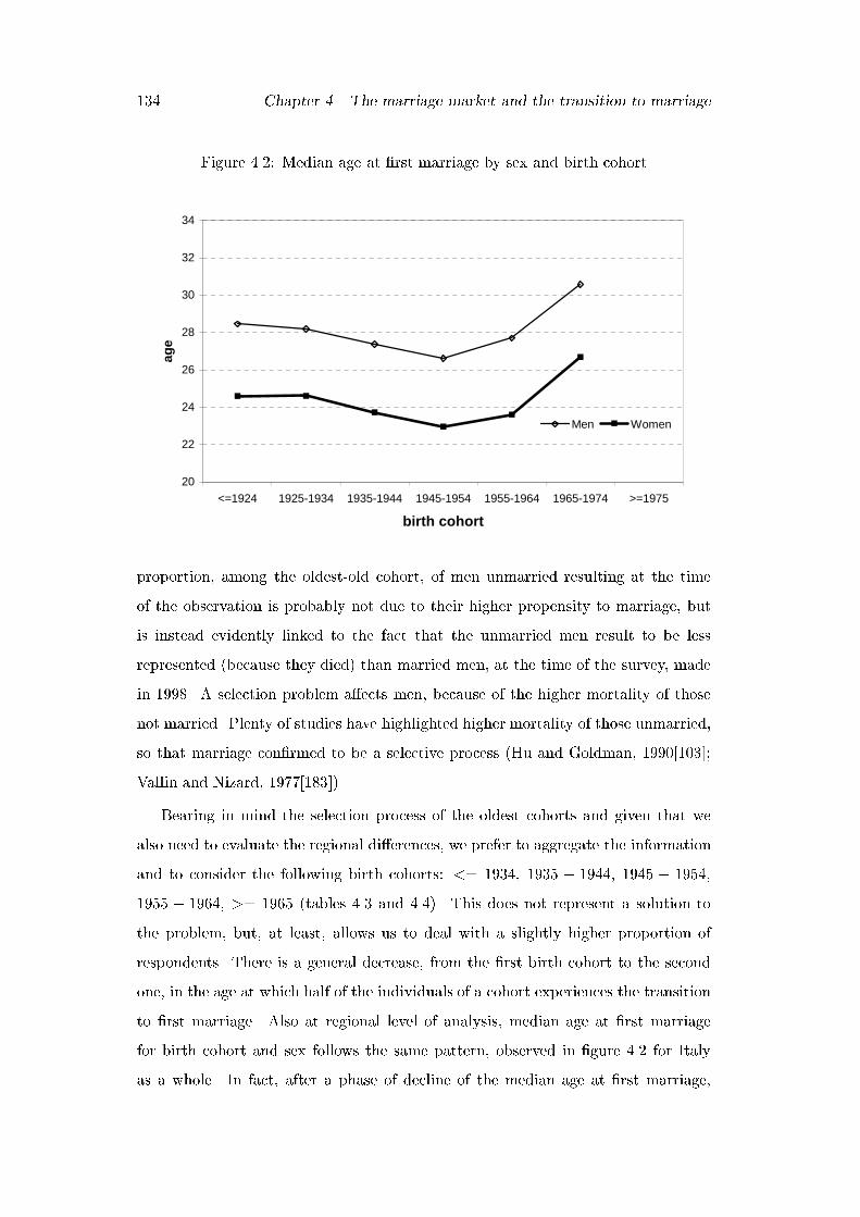
134 Chapter 4. The marriage market and the transition to marriage
Figure 4.2: Median age at �rst marriage by sex and birth cohort
20
22
24
26
28
30
32
34
<=1924 1925-1934 1935-1944 1945-1954 1955-1964 1965-1974 >=1975
birth cohort
age
Men Women
proportion, among the oldest-old cohort, of men unmarried resulting at the time
of the observation is probably not due to their higher propensity to marriage, but
is instead evidently linked to the fact that the unmarried men result to be less
represented (because they died) than married men, at the time of the survey, made
in 1998. A selection problem a�ects men, because of the higher mortality of those
not married. Plenty of studies have highlighted higher mortality of those unmarried,
so that marriage con�rmed to be a selective process (Hu and Goldman, 1990[103];
Vallin and Nizard, 1977[183]).
Bearing in mind the selection process of the oldest cohorts and given that we
also need to evaluate the regional di�erences, we prefer to aggregate the information
and to consider the following birth cohorts: <= 1934, 1935 � 1944, 1945 � 1954,
1955 � 1964, >= 1965 (tables 4.3 and 4.4). This does not represent a solution to
the problem, but, at least, allows us to deal with a slightly higher proportion of
respondents. There is a general decrease, from the �rst birth cohort to the second
one, in the age at which half of the individuals of a cohort experiences the transition
to �rst marriage. Also at regional level of analysis, median age at �rst marriage
for birth cohort and sex follows the same pattern, observed in �gure 4.2 for Italy
as a whole. In fact, after a phase of decline of the median age at �rst marriage,
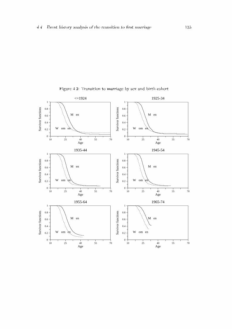
4.4. Event history analysis of the transition to �rst marriage 135
Figure 4.3: Transition to marriage by sex and birth cohort
10 25 40 55 700
0.2
0.4
0.6
0.8
11955-64
Age
Surv
ivor
fun
ctio
ns
M en
W om en
10 25 40 55 700
0.2
0.4
0.6
0.8
11965-74
Age
Surv
ivor
fun
ctio
ns
M en
W om en
10 25 40 55 700
0.2
0.4
0.6
0.8
11935-44
Age
Surv
ivor
fun
ctio
ns
M en
W om en
10 25 40 55 700
0.2
0.4
0.6
0.8
11945-54
Age
Surv
ivor
fun
ctio
ns
M en
W om en
10 25 40 55 700
0.2
0.4
0.6
0.8
1<=1924
Age
Surv
ivor
fun
ctio
ns
M en
W om en
10 25 40 55 700
0.2
0.4
0.6
0.8
11925-34
Age
Surv
ivor
fun
ctio
nsM en
W om en

136 Chapter 4. The marriage market and the transition to marriage
Table 4.3: Survivor function quartiles for marriage by sex, birth cohort and territo-
rial division at birth
territorialdivision quartiles <=1934 1935-44 1945-54 1955-64 >=1965 <=1934 1935-44 1945-54 1955-64 >=1965
1st quartile 25.9 25.1 24.2 25.1 27.5 22.1 21.8 21.1 21.1 24.2NORTH median 28.7 27.1 26.4 28.3 31.2 25.0 24.1 23.1 24.0 28.0
3rd quartile 32.7 30.6 30.2 34.6 29.1 27.0 26.0 28.1
1st quartile 25.1 25.2 24.4 25.1 27.6 21.1 21.3 20.6 21.1 24.3CENTRE median 28.0 27.2 26.6 28.2 31.0 23.9 23.4 22.6 23.9 28.0
3rd quartile 31.3 30.2 29.5 31.8 27.9 26.1 25.4 27.7
1st quartile 24.7 24.5 24.3 24.5 26.1 21.0 20.6 20.2 20.2 22.2SOUTH median 28.0 27.4 26.8 27.2 29.9 24.5 23.2 23.0 23.0 25.9
3rd quartile 32.0 30.3 30.1 31.2 29.7 27.2 26.7 27.1 30.5
1st quartile 25.2 24.9 24.3 24.8 27.0 21.5 21.3 20.7 20.7 23.3ITALY median 28.3 27.2 26.6 27.7 30.6 24.6 23.7 22.9 23.6 27.2
3rd quartile 32.2 30.4 30.0 32.2 29.1 26.9 26.2 27.5
MEN WOMEN
which involved all birth cohorts up to 1945-54, a phase of sensible increase has
been observed. The 1945-1954 birth cohort marks a turning point in the marital
behaviour: it is characterised by an anticipatory marital behaviour which will be
perceivable during the 1970s.
Afterwards, it should be highlighted that the major (highest) postponement
with respect to the previous birth cohorts' behaviour has been experienced by the
youngest cohort born after 1965: half of the men (women) in this birth cohort
survived to �rst marriage on average 3(4) years more, in the median age, than the
previous birth cohort. This trend holds also at regional level of analysis (table 4.3)
even though the South has a small delay in that. A postponement process for
the cohort born after 1945-54 emerges also at every stage of the transition to �rst
marriage: so that the �rst quartile shows the postponement of the age at which
25% of people have experienced a marriage. For the South such a postponement is
weaker than for the North and the Centre (table 4.3).
In table 4.4, we show that the proportions of survivors to marriage at selected
ages, have �rst dropped, up to cohort 1945-54, and then quickly risen, therefore
following the pattern already described by the median duration of �rst marriage.
Marriage was more frequent and took place earlier for men and women born during
the 1930s: then the proportion of unmarried at every age fell continuously up to the
birth cohort 1946-55. For those born at the end of the 1950s and early 1960s we
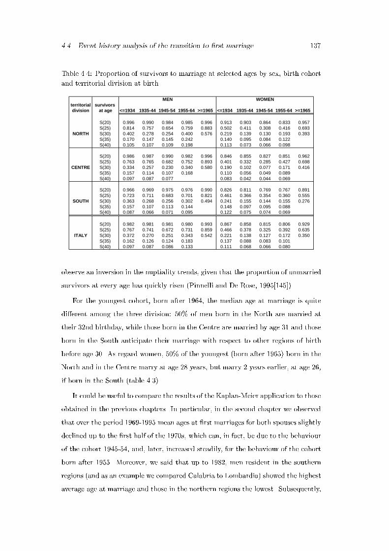
4.4. Event history analysis of the transition to �rst marriage 137
Table 4.4: Proportion of survivors to marriage at selected ages by sex, birth cohort
and territorial division at birth
territorial survivors
division at age <=1934 1935-44 1945-54 1955-64 >=1965 <=1934 1935-44 1945-54 1955-64 >=1965
S(20) 0.996 0.990 0.984 0.985 0.996 0.913 0.903 0.864 0.833 0.957S(25) 0.814 0.757 0.654 0.759 0.883 0.502 0.411 0.308 0.416 0.693
NORTH S(30) 0.402 0.278 0.254 0.400 0.576 0.219 0.139 0.130 0.193 0.393S(35) 0.170 0.147 0.145 0.242 0.140 0.095 0.084 0.122S(40) 0.105 0.107 0.109 0.198 0.113 0.073 0.066 0.098
S(20) 0.986 0.987 0.990 0.982 0.996 0.846 0.855 0.827 0.851 0.962S(25) 0.763 0.765 0.682 0.752 0.893 0.401 0.332 0.285 0.427 0.698
CENTRE S(30) 0.334 0.257 0.230 0.340 0.580 0.190 0.102 0.077 0.171 0.416S(35) 0.157 0.114 0.107 0.168 0.110 0.056 0.049 0.089S(40) 0.097 0.087 0.077 0.083 0.042 0.044 0.069
S(20) 0.966 0.969 0.975 0.976 0.990 0.826 0.811 0.769 0.767 0.891S(25) 0.723 0.711 0.683 0.701 0.821 0.461 0.366 0.354 0.360 0.555
SOUTH S(30) 0.363 0.268 0.256 0.302 0.494 0.241 0.155 0.144 0.155 0.276S(35) 0.157 0.107 0.113 0.144 0.148 0.097 0.095 0.088S(40) 0.087 0.066 0.071 0.095 0.122 0.075 0.074 0.069
S(20) 0.982 0.981 0.981 0.980 0.993 0.867 0.858 0.815 0.806 0.929S(25) 0.767 0.741 0.672 0.731 0.859 0.466 0.378 0.325 0.392 0.635
ITALY S(30) 0.372 0.270 0.251 0.343 0.542 0.221 0.138 0.127 0.172 0.350S(35) 0.162 0.126 0.124 0.183 0.137 0.088 0.083 0.101S(40) 0.097 0.087 0.086 0.133 0.111 0.068 0.066 0.080
MEN WOMEN
observe an inversion in the nuptiality trends, given that the proportion of unmarried
survivors at every age has quickly risen (Pinnelli and De Rose, 1995[145]).
For the youngest cohort, born after 1964, the median age at marriage is quite
di�erent among the three division: 50% of men born in the North are married at
their 32nd birthday, while those born in the Centre are married by age 31 and those
born in the South anticipate their marriage with respect to other regions of birth
before age 30. As regard women, 50% of the youngest (born after 1965) born in the
North and in the Centre marry at age 28 years, but marry 2 years earlier, at age 26,
if born in the South (table 4.3).
It could be useful to compare the results of the Kaplan-Meier application to those
obtained in the previous chapters. In particular, in the second chapter we observed
that over the period 1969-1995 mean ages at �rst marriages for both spouses slightly
declined up to the �rst half of the 1970s, which can, in fact, be due to the behaviour
of the cohort 1945-54, and, later, increased steadily, for the behaviour of the cohort
born after 1955. Moreover, we said that up to 1982, men resident in the southern
regions (and as an example we compared Calabria to Lombardia) showed the highest
average age at marriage and those in the northern regions the lowest. Subsequently,
138 Chapter 4. The marriage market and the transition to marriage
a shift took place so that men in the South kept a lower age at �rst marriage than all
other Italians. The event history analysis conducted on the birth cohorts represented
in table 4.3 and 4.4 con�rms our previous �ndings: as regard men, the median age
at �rst marriage in the South was higher than in the North and in the Centre for
birth cohort 1935-55 and 1945-54, but from the cohort born in 1955 it continues to
be the lowest. Also the growing di�erentiation in the timing of the marriage among
regions can be con�rmed by the longitudinal analysis resulting from the Kaplan-
Meier method: over time a widening di�erence in the ages at �rst marriage can be
observed among territorial divisions. For each sex, median ages at �rst marriage,
which are very close for the old birth cohort (small di�erences are of about one year
over the country), show a growing di�erence among macroregions for the young
cohorts, for instance, women born after 1965 in the South marry 2.1 years earlier
than those born in the North and in the Centre (table 4.3).
In �gure 4.4, patterns of transition to marriage are reported for men and women,
and by cohort and division of birth. To make the reading easier, let us remember
that the continue line corresponds to the North, the dotted line to the Centre and
the dashed line to the South. Starting from a quite di�erentiated situation among
macroregions of birth, for those born before 1934, men gradually assume a behaviour
characterised by a lower variability between divisions of birth. While for the birth
cohort <= 1934 men born in the Centre enter into �rst marriage slightly after the
southern men and slightly before the northern ones, for the cohort born in 1945-54,
which is also the one with the lowest proportions of survivals at marriage to all
ages (therefore with the quickest transition to �rst marriage), patterns are rather
undi�erentiated by division of birth. From cohorts born during 1955-64 emerges the
anticipatory behaviour of the southern regions when compared to the northern and
central ones. Women in the South, indicated by the dashed line, enter early into
�rst marriage, while central and northern ones marry slightly later. However, at
around age 24 the dotted line, being the lowest line and corresponding to women
born in Central regions, indicates a pattern of high transition to �rst marriage up
to cohort 1945-54. From the cohort born in 1955-64 the South shows a pattern
characterised by a quick transition to marriage, reached by the Central women only
at around age 40. Lastly, the youngest cohorts of women, born after 1965, clearly

4.5. Evaluating the impact of the marriage squeeze 139
show a gap between the marital behaviour of the southern women on the one hand,
in comparison to that of the northern and central ones, which is postponed and
overlapped on the other hand: there is now a clear fork between the curves. The
youngest birth cohorts are censored by the interview and therefore their patterns,
which is anyway characterised by a later entry into �rst marriage with respect to
previous birth cohorts, is just perceivable (cohort born after 1965).
Overall, across cohorts there has been a slight anticipation of the age at marriage
for those born in the years 1945-54 and a rise of the age at �rst marriage for the
successive cohorts (see also �gure 4.2).
4.5 Evaluating the impact of the marriage squeeze
In order to evaluate the impact of the di�erential imbalances on �rst marriage be-
tween sexes, we apply event history models including the measure of the squeeze
in the marriage market as a time-varying covariate. As we said, individual survey
data have been linked to the three alternative measures of the squeeze (S, I and
Ifreq) computed both according to the region of birth of the individuals and to that
of their residence at the time of the survey. Our main purposes are either to look
for an e�ect of the squeeze and to ascertain whether there is a time dependence
of the e�ect of the squeeze, controlling for regional di�erences. Here, the focus is
on a set of cohorts whose life-courses are not censored at an early age: cohorts of
individuals born in the period 1955-1964 have been chosen to evaluate the e�ect of
the imbalances on the marriage market.
I) In particular, we would expect that increasing the measure of the squeeze,
which entails a worsening of the conditions for women, could a�ect the mar-
riage opportunities of both sexes di�erently. In fact,
a) a squeeze against women de�nitely put them in a worse position, length-
ening the spell, the duration of the time interval necessary to �nd an
appropriate partner,
b) on the other way round, a squeeze against women, speed up the mating
opportunities of men.

140 Chapter 4. The marriage market and the transition to marriage
Figure 4.4: Survivor functions by sex, cohort and macroregion of birth. ITALY
10 20 30 40 50 60 700
0.2
0.4
0.6
0.8
1M en, >=1965
Age
Surv
ivor
func
tions N
C
S
10 20 30 40 50 60 700
0.2
0.4
0.6
0.8
1W om en, >=1965
Age
Surv
ivor
func
tions N
C
S
10 20 30 40 50 60 700
0.2
0.4
0.6
0.8
1M en, 1955-64
Age
Surv
ivor
func
tions
N
C
S
10 20 30 40 50 60 700
0.2
0.4
0.6
0.8
1W om en, 1955-64
Age
Surv
ivor
func
tions
N
C
S
10 20 30 40 50 60 700
0.2
0.4
0.6
0.8
1M en, 1945-54
Age
Surv
ivor
func
tions
NC
S
10 20 30 40 50 60 700
0.2
0.4
0.6
0.8
1W om en, 1945-54
Age
Surv
ivor
func
tions
N
C
S
10 20 30 40 50 60 700
0.2
0.4
0.6
0.8
1M en, 1935-44
Age
Surv
ivor
func
tions
N C
S
10 20 30 40 50 60 700
0.2
0.4
0.6
0.8
1W om en, 1935-44
Age
Surv
ivor
func
tions N
C
S
10 20 30 40 50 60 700
0.2
0.4
0.6
0.8
1M en, <=1934
Age
Surv
ivor
func
tions
N C
S
10 20 30 40 50 60 700
0.2
0.4
0.6
0.8
1W om en, <=1934
Age
Surv
ivor
func
tions N
C
S

4.5. Evaluating the impact of the marriage squeeze 141
II) As a second step, we are interested in analysing the possibility that the impact
of the squeeze might not be constant, but might indeed change over time. This
implies the existence of an age pattern of the squeeze and, in this case, our
expectations are the following.
a) For men, we would expect to �nd an acceleration in the marital behavior
improving the marriage opportunities at all ages, especially for those
which are normally less exposed to the risk of marriage. This means that
perhaps, young men could take advantage of a situation characterised by
a squeeze against women.
b) As regard women, we might expect that, even in the case of a squeeze
against them, they are not entirely excluded from the process of assorta-
tive mating: the matching process will require more time for lots of them,
so that the outcome will be a general postponement e�ect.
We also expect that the three measures analysed in the previous chapter, S, I and
Ifreq, do not behave di�erently, given that they are descriptive of the same phe-
nomenon. Modeling the transition to �rst marriage by using this measures provides
us with a test of their robustness: among other things, we also wish to test whether
I and Ifreq, though built in a simplistic way, succeed in describing the imbalance in
the marriage market as S would do.
In evaluating a nested model's performance we use the likelihood-ratio test com-
paring each model to a reference model. To compare nonnested models we make use
of the Bayesian Information Criterion (BIC) (see appendix). Theoretical explana-
tions of the models can be found in the mathematical appendix, as well.
4.5.1 Proportional hazards model
To start with we could try to evaluate the e�ects of observed covariates without
specifying a time period e�ect: a semi-parametric model of the Cox type. The Cox
model is also known as semi-parametric because it does not specify the parametric
distribution for describing the transition rate dependence on time. This model
emphasises the role of the covariates in explaining a change in the transition rate to
�rst marriage: covariates represent our knowledge about the observed heterogeneity

142 Chapter 4. The marriage market and the transition to marriage
of the population. One of its features is that it is based on the proportionality
assumption, according to which two units of analysis have proportional e�ects on
the basis of the speci�ed baseline rate and a speci�c e�ect. At each point in time,
the ratio of the e�ect of being in a covariate category relative to another is constant.
In other words, \the e�ects of covariates can only induce proportional shifts in the
transition rate but cannot change its shape" (Blossfeld and Rohwer, 1995[24, p.212]).
The proportionality assumption implies that the duration of exposure has the same
impact on each individual, suggesting that the probability of experiencing the life
event (�rst marriage) varies over time in the same way for each respondent11.
In our case, region of residence at the time of the survey (1998) or at birth are
our covariates, and their e�ects are assumed to be independent from time. The
purpose here is to show whether the marriage market situation explains part of the
regional level di�erences. Sixteen models are presented: they control for the region
of residence at the time of the survey and at birth (tables 4.5 and 4.6 respectively) for
men and women, and, apart from Model I (basically used to check the improvement
of the other ones), Model II includes S as a covariate, Model III includes I and
Model IV includes Ifreq.
In particular, the equation which expresses the transition rate r(t) as a function
of the baseline rate r0(t) and of the covariates X1 (region) and X2 (imbalance)12, is
the following:
r(t) = r0(t) exp(�1X1 + �2X2) (4.1)
Comparing each of the models with an alternative measure of the squeeze (S; I; Ifreq),
to the �rst one, which exclude X2 it emerges that for men, the squeeze measures,
positive over time, have no signi�cant e�ects13(table 4.5, �rst part). The positive
11For more details about the model see the appendix.12Region is a categorical variable, therefore X1 is a vector of dummy variables
X1=(Piedmont,. . . Sardinia); the measure of the squeeze is a continuous variable, therefore X2
assumes value in R.13It is normally of primary interest to test whether the parameter �i is signi�cantly not di�erent
from zero. The signi�cance level reported in this and in the following tables corresponds to 1-p-
value. The p-value represents the probability that the sample value would be as large as the value
actually observed, if the null hypothesis (�i = 0) is true. Therefore when in the column `Signif' we
have 1.000 it means that our coe�cient has a p-value equals to 0.000. The � coe�cients are the
logarithm of the hazard ratio r(t)=r0(t) and any value of � in the range (�1;1) will lead to a
positive value of the hazard ratio. Note that positive values of � are obtained when the hazard ratio
is greater than unity. An increase in a unity of Xi makes multiply the transition rate by exp(�i)
(for more details on the interpretation of the parameters see in appendix).

4.5. Evaluating the impact of the marriage squeeze 143
sign of the e�ect for men of a female disadvantage in the marriage market con-
�rms our expectations. In turn, the squeeze for women, whichever be the measure
adopted, has always a negative and signi�cant e�ect (table 4.5, second part). This
means that, if the squeeze increases (S, I or Ifreq positive) then we have a negative
e�ect for women, therefore they postpone marriage, at every time of their lives.
Furthermore, men resident in the North-Centre and Sardinia have slow transition to
�rst marriage, while those resident in the South experience marriage sooner. Also
women resident in the North-Centre of Italy have a slow transition to �rst marriage
(table 4.5). However, in the next models, we will not go in depth in the analysis
of the regional di�erences, we will mainly use them as control variables. According
to the Bayesian Information Criterion (BIC) used to compare `nonnested models',
for women the Model III, which uses the index I, is slightly better than previous
others. Models controlling the region of birth of the individuals are reported in
table 4.6, where we observe a situation similar to the previous one: all the measures
of the squeeze show a positive e�ect, but not signi�cant, for men while for women
it is negative and always signi�cant. As concerns the regions e�ect a clear cut be-
haviour is more straightforward. In fact, both women and men born in the North
or in the Centre have a slower transition for �rst marriage than the baseline one,
while the South (except Sardinia) they have a faster one. According to the BIC the
best model in table 4.6 is the fourth for both sexes, therefore the best measure to
represent the squeeze is Ifreq.
As the model by region of birth and that by region of residence refer to dif-
ferent amounts of individuals14, they cannot be compared using the BIC measure
computed here.
All in all we can say that the proportional hazards model works better for women
than for men. While for the former there is a clear decreasing probability of marrying
in a situation characterised by their disadvantage, for the latter does not emerge a
signi�cant increase in the marriage opportunities. On the other hand, it should be
highlighted that this model is very useful in case the proportionality assumption is
respected. In other cases, it could simply be that the existence of an age-dependence
14It is necessary to remember that for the region of birth we excluded respondent born abroad
or with a missing value for their region of birth.

144 Chapter 4. The marriage market and the transition to marriage
Table 4.5: Cox models by sex and for alternative measures of the squeeze; by region
of residence in 1998
REGION OF RESIDENCE AT THE TIME OF THE SURVEYMEN
Coeff S.E. Signif Coeff S.E. Signif Coeff S.E. Signif Coeff S.E. Signif
Piedmont (base)Vaa -0.3056 0.1345 0.9770 -0.3446 0.1377 0.9876 -0.3446 0.1377 0.9876 -0.3400 0.1374 0.9867Lom 0.0280 0.0805 0.2716 0.0206 0.0807 0.2012 0.0206 0.0807 0.2013 0.0214 0.0807 0.2087Taa -0.2236 0.0992 0.9758 -0.1967 0.1012 0.9480 -0.1967 0.1012 0.9480 -0.1990 0.1011 0.9509Ven -0.0949 0.0891 0.7131 -0.0864 0.0893 0.6668 -0.0864 0.0893 0.6668 -0.0872 0.0893 0.6710Fvg -0.1208 0.1073 0.7394 -0.1098 0.1076 0.6924 -0.1098 0.1076 0.6924 -0.1107 0.1076 0.6960Lig -0.3902 0.1123 0.9995 -0.3760 0.1128 0.9991 -0.3761 0.1128 0.9991 -0.3772 0.1127 0.9992Tos 0.0247 0.0895 0.2172 0.0035 0.0909 0.0310 0.0035 0.0909 0.0310 0.0058 0.0908 0.0508Umb -0.0298 0.1071 0.2195 -0.0545 0.1086 0.3842 -0.0545 0.1086 0.3842 -0.0520 0.1085 0.3682Er -0.1711 0.0966 0.9234 -0.1832 0.0970 0.9409 -0.1832 0.0970 0.9409 -0.1820 0.0970 0.9394
Mar -0.0440 0.0968 0.3505 -0.0654 0.0981 0.4948 -0.0654 0.0981 0.4947 -0.0641 0.0981 0.4865Laz -0.0053 0.0918 0.0457 -0.0542 0.0988 0.4166 -0.0542 0.0988 0.4166 -0.0494 0.0984 0.3841Abr 0.1660 0.0935 0.9241 0.1386 0.0957 0.8524 0.1386 0.0957 0.8524 0.1410 0.0957 0.8594Mol 0.1123 0.1046 0.7172 0.1215 0.1048 0.7536 0.1215 0.1048 0.7536 0.1220 0.1049 0.7552Cam 0.0797 0.0845 0.6546 0.0737 0.0846 0.6165 0.0737 0.0846 0.6165 0.0751 0.0845 0.6255Pug 0.2393 0.0824 0.9963 0.2120 0.0849 0.9874 0.2120 0.0849 0.9874 0.2131 0.0851 0.9878Bas -0.1193 0.1145 0.7024 -0.1144 0.1146 0.6820 -0.1144 0.1146 0.6820 -0.1138 0.1146 0.6794Cal 0.0957 0.0885 0.7205 0.1102 0.0891 0.7836 0.1102 0.0891 0.7836 0.1099 0.0892 0.7820Sic 0.1643 0.0854 0.9457 0.1335 0.0885 0.8687 0.1335 0.0885 0.8687 0.1325 0.0891 0.8630Sar -0.1334 0.0994 0.8205 -0.1295 0.0994 0.8072 -0.1295 0.0994 0.8072 -0.1295 0.0994 0.8071
SQUEEZE:S 1.4457 1.0827 0.8182I 2.8897 2.1647 0.8181
Ifreq 2.2297 1.7920 0.7866
n. parameters: 19 20 20 20n. events 3921Log-likelihood: -30587.60 -30586.71 -30586.71 -30586.83BIC: 1.804 1.805 2.040
REGION OF RESIDENCE AT THE TIME OF THE SURVEYWOMEN
Coeff S.E. Signif Coeff S.E. Signif Coeff S.E. Signif Coeff S.E. Signif
Piedmont (base)Vaa -0.2601 0.1165 0.9744 -0.1772 0.1170 0.8700 -0.1773 0.1170 0.8702 -0.1941 0.1168 0.9036Lom -0.1508 0.0739 0.9588 -0.1117 0.0742 0.8679 -0.1117 0.0742 0.8679 -0.1155 0.0741 0.8810Taa -0.2762 0.0919 0.9973 -0.3928 0.0942 1.0000 -0.3928 0.0942 1.0000 -0.3885 0.0940 1.0000Ven -0.1803 0.0830 0.9702 -0.2089 0.0832 0.9880 -0.2089 0.0832 0.9880 -0.2094 0.0832 0.9882Fvg -0.0505 0.0940 0.4090 -0.1527 0.0959 0.8886 -0.1527 0.0959 0.8888 -0.1542 0.0960 0.8918Lig -0.4513 0.1019 1.0000 -0.5067 0.1024 1.0000 -0.5067 0.1024 1.0000 -0.5046 0.1024 1.0000Tos -0.0636 0.0810 0.5673 0.0112 0.0821 0.1085 0.0112 0.0821 0.1083 0.0032 0.0818 0.0311Umb -0.2363 0.1003 0.9815 -0.1764 0.1008 0.9199 -0.1765 0.1008 0.9199 -0.1854 0.1007 0.9345Er -0.1956 0.0833 0.9811 -0.1309 0.0841 0.8808 -0.1310 0.0841 0.8808 -0.1356 0.0840 0.8936
Mar -0.0488 0.0883 0.4195 0.0335 0.0894 0.2923 0.0335 0.0894 0.2922 0.0316 0.0894 0.2766Laz -0.1279 0.0838 0.8731 0.0597 0.0899 0.4938 0.0598 0.0899 0.4938 0.0454 0.0890 0.3901Abr -0.0195 0.0850 0.1811 0.0571 0.0860 0.4935 0.0571 0.0860 0.4934 0.0500 0.0858 0.4401Mol -0.0780 0.1019 0.5559 -0.1300 0.1023 0.7961 -0.1300 0.1023 0.7960 -0.1321 0.1023 0.8031Cam -0.0604 0.0800 0.5496 -0.0387 0.0801 0.3707 -0.0387 0.0801 0.3708 -0.0446 0.0801 0.4229Pug -0.0101 0.0776 0.1034 0.1051 0.0801 0.8101 0.1051 0.0801 0.8101 0.1045 0.0801 0.8081Bas -0.0788 0.1061 0.5425 -0.0868 0.1061 0.5868 -0.0868 0.1061 0.5867 -0.0868 0.1061 0.5864Cal 0.1255 0.0817 0.8756 0.0435 0.0830 0.4000 0.0435 0.0830 0.4000 0.0406 0.0831 0.3745Sic 0.0018 0.0782 0.0184 0.1253 0.0812 0.8772 0.1253 0.0812 0.8772 0.1336 0.0816 0.8984Sar -0.2582 0.0924 0.9948 -0.2604 0.0924 0.9952 -0.2604 0.0924 0.9952 -0.2593 0.0924 0.9950
SQUEEZE:S -5.4209 0.9459 1.0000I -10.8375 1.8908 1.0000
Ifreq -8.3583 1.4606 1.0000
n. parameters: 19 20 20 20n. events 4530Log -likelihood: -35199.1 -35182.91 -35182.91 -35183.04BIC: -28.724 -28.733 -28.466
Model IV
Model I Model II Model III Model IV
Model I Model II Model III
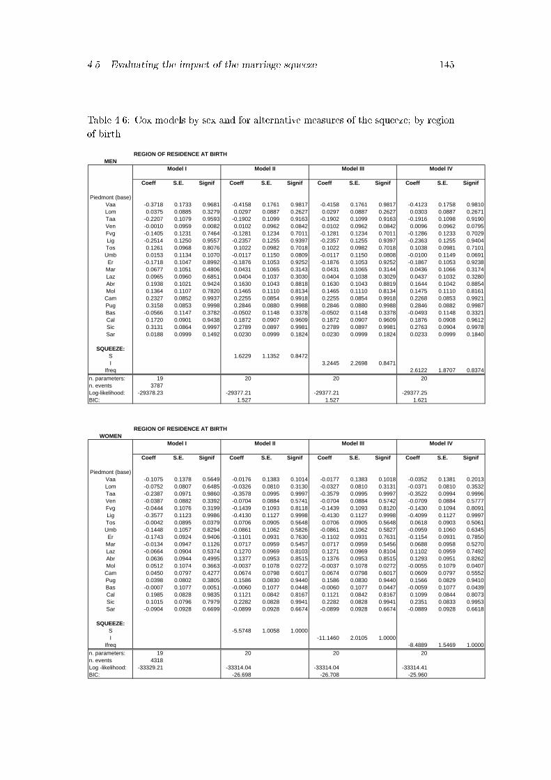
4.5. Evaluating the impact of the marriage squeeze 145
Table 4.6: Cox models by sex and for alternative measures of the squeeze; by region
of birth
REGION OF RESIDENCE AT BIRTHMEN
Coeff S.E. Signif Coeff S.E. Signif Coeff S.E. Signif Coeff S.E. Signif
Piedmont (base)Vaa -0.3718 0.1733 0.9681 -0.4158 0.1761 0.9817 -0.4158 0.1761 0.9817 -0.4123 0.1758 0.9810Lom 0.0375 0.0885 0.3279 0.0297 0.0887 0.2627 0.0297 0.0887 0.2627 0.0303 0.0887 0.2671Taa -0.2207 0.1079 0.9593 -0.1902 0.1099 0.9163 -0.1902 0.1099 0.9163 -0.1916 0.1098 0.9190Ven -0.0010 0.0959 0.0082 0.0102 0.0962 0.0842 0.0102 0.0962 0.0842 0.0096 0.0962 0.0795Fvg -0.1405 0.1231 0.7464 -0.1281 0.1234 0.7011 -0.1281 0.1234 0.7011 -0.1286 0.1233 0.7029Lig -0.2514 0.1250 0.9557 -0.2357 0.1255 0.9397 -0.2357 0.1255 0.9397 -0.2363 0.1255 0.9404Tos 0.1261 0.0968 0.8076 0.1022 0.0982 0.7018 0.1022 0.0982 0.7018 0.1038 0.0981 0.7101Umb 0.0153 0.1134 0.1070 -0.0117 0.1150 0.0809 -0.0117 0.1150 0.0808 -0.0100 0.1149 0.0691Er -0.1718 0.1047 0.8992 -0.1876 0.1053 0.9252 -0.1876 0.1053 0.9252 -0.1867 0.1053 0.9238
Mar 0.0677 0.1051 0.4806 0.0431 0.1065 0.3143 0.0431 0.1065 0.3144 0.0436 0.1066 0.3174Laz 0.0965 0.0960 0.6851 0.0404 0.1037 0.3030 0.0404 0.1038 0.3029 0.0437 0.1032 0.3280Abr 0.1938 0.1021 0.9424 0.1630 0.1043 0.8818 0.1630 0.1043 0.8819 0.1644 0.1042 0.8854Mol 0.1364 0.1107 0.7820 0.1465 0.1110 0.8134 0.1465 0.1110 0.8134 0.1475 0.1110 0.8161Cam 0.2327 0.0852 0.9937 0.2255 0.0854 0.9918 0.2255 0.0854 0.9918 0.2268 0.0853 0.9921Pug 0.3158 0.0853 0.9998 0.2846 0.0880 0.9988 0.2846 0.0880 0.9988 0.2846 0.0882 0.9987Bas -0.0566 0.1147 0.3782 -0.0502 0.1148 0.3378 -0.0502 0.1148 0.3378 -0.0493 0.1148 0.3321Cal 0.1720 0.0901 0.9438 0.1872 0.0907 0.9609 0.1872 0.0907 0.9609 0.1876 0.0908 0.9612Sic 0.3131 0.0864 0.9997 0.2789 0.0897 0.9981 0.2789 0.0897 0.9981 0.2763 0.0904 0.9978Sar 0.0188 0.0999 0.1492 0.0230 0.0999 0.1824 0.0230 0.0999 0.1824 0.0233 0.0999 0.1840
SQUEEZE:S 1.6229 1.1352 0.8472I 3.2445 2.2698 0.8471
Ifreq 2.6122 1.8707 0.8374
n. parameters: 19 20 20 20n. events 3787Log-likelihood: -29378.23 -29377.21 -29377.21 -29377.25BIC: 1.527 1.527 1.621
REGION OF RESIDENCE AT BIRTHWOMEN
Coeff S.E. Signif Coeff S.E. Signif Coeff S.E. Signif Coeff S.E. Signif
Piedmont (base)Vaa -0.1075 0.1378 0.5649 -0.0176 0.1383 0.1014 -0.0177 0.1383 0.1018 -0.0352 0.1381 0.2013Lom -0.0752 0.0807 0.6485 -0.0326 0.0810 0.3130 -0.0327 0.0810 0.3131 -0.0371 0.0810 0.3532Taa -0.2387 0.0971 0.9860 -0.3578 0.0995 0.9997 -0.3579 0.0995 0.9997 -0.3522 0.0994 0.9996Ven -0.0387 0.0882 0.3392 -0.0704 0.0884 0.5741 -0.0704 0.0884 0.5742 -0.0709 0.0884 0.5777Fvg -0.0444 0.1076 0.3199 -0.1439 0.1093 0.8118 -0.1439 0.1093 0.8120 -0.1430 0.1094 0.8091Lig -0.3577 0.1123 0.9986 -0.4130 0.1127 0.9998 -0.4130 0.1127 0.9998 -0.4099 0.1127 0.9997Tos -0.0042 0.0895 0.0379 0.0706 0.0905 0.5648 0.0706 0.0905 0.5648 0.0618 0.0903 0.5061Umb -0.1448 0.1057 0.8294 -0.0861 0.1062 0.5826 -0.0861 0.1062 0.5827 -0.0959 0.1060 0.6345Er -0.1743 0.0924 0.9406 -0.1101 0.0931 0.7630 -0.1102 0.0931 0.7631 -0.1154 0.0931 0.7850
Mar -0.0134 0.0947 0.1126 0.0717 0.0959 0.5457 0.0717 0.0959 0.5456 0.0688 0.0958 0.5270Laz -0.0664 0.0904 0.5374 0.1270 0.0969 0.8103 0.1271 0.0969 0.8104 0.1102 0.0959 0.7492Abr 0.0636 0.0944 0.4995 0.1377 0.0953 0.8515 0.1376 0.0953 0.8515 0.1293 0.0951 0.8262Mol 0.0512 0.1074 0.3663 -0.0037 0.1078 0.0272 -0.0037 0.1078 0.0272 -0.0055 0.1079 0.0407Cam 0.0450 0.0797 0.4277 0.0674 0.0798 0.6017 0.0674 0.0798 0.6017 0.0609 0.0797 0.5552Pug 0.0398 0.0802 0.3805 0.1586 0.0830 0.9440 0.1586 0.0830 0.9440 0.1566 0.0829 0.9410Bas -0.0007 0.1077 0.0051 -0.0060 0.1077 0.0448 -0.0060 0.1077 0.0447 -0.0059 0.1077 0.0439Cal 0.1985 0.0828 0.9835 0.1121 0.0842 0.8167 0.1121 0.0842 0.8167 0.1099 0.0844 0.8073Sic 0.1015 0.0796 0.7979 0.2282 0.0828 0.9941 0.2282 0.0828 0.9941 0.2351 0.0833 0.9953Sar -0.0904 0.0928 0.6699 -0.0899 0.0928 0.6674 -0.0899 0.0928 0.6674 -0.0889 0.0928 0.6618
SQUEEZE:S -5.5748 1.0058 1.0000I -11.1460 2.0105 1.0000
Ifreq -8.4889 1.5469 1.0000
n. parameters: 19 20 20 20n. events 4318Log -likelihood: -33329.21 -33314.04 -33314.04 -33314.41BIC: -26.698 -26.708 -25.960
Model I Model II Model III Model IV
Model I Model II Model III Model IV
146 Chapter 4. The marriage market and the transition to marriage
pattern does not emerge because it is confounded by compensating factors. The
following analyses attempt to ascertain this point by further modeling the transition
rate.
4.5.2 The piecewise constant exponential model
Assuming that the e�ects of the marriage market are proportional over time is, in
most applications of transition rate models, not theoretically justi�ed. For an appro-
priate modeling it is often crucial to include time-dependent covariates in transition
rate models. The piecewise constant exponential model allows for the subdivision
of the time-axis in a subset of intervals of analysis within which the transition rate
is considered to be constant. It provides a baseline function, expressing the time-
dependence of the process. As regards the e�ects of the covariates, the model gives
us two possibilities, that we will see better later. To practical purposes, this ap-
proach appears to be particularly useful especially when the researcher is not in the
position to directly include time-dependent covariates, or when s/he does not have a
clear idea of the form of the time-dependence of the process (Blossfeld and Rohwer,
1995[24]).
If there are m time periods, the distribution of durations has m parameters15. In
particular, we used to split the time axis di�erently between the sexes: for men we
chose the ages 23, 25, 27, 29, 32 and for women the ages 18, 20, 22, 24, 26, 28, 30.
The choice of the time split has been based on the criterion to gather approximately
an equivalent amount of events in each interval.
There are two possible ways to include covariates. We can, for instance, assume
that only a baseline rate, given by period-speci�c constants, can vary across time
periods and, therefore, the covariates have the same (proportional) e�ects in each
period (as they do not vary with time). Another way could be to allow for period-
speci�c e�ects of covariates also. Having divided the time axis into m time periods,
15The choice of an appropriate number of intervals is subject to speci�c considerations. Evidently,
the more the intervals, the best the approximation of the unknown baseline rate, but this implies
a large number of coe�cients to be estimated. On the other hand, a small number of intervals is
less problematic as concern the estimations, but provides a rough approximation of the baseline
rate. Therefore, it is wise to search for a compromise between the two alternatives. Another obvious
requirement is building intervals with ending times for some episodes: that is to say, intervals should
contain events.
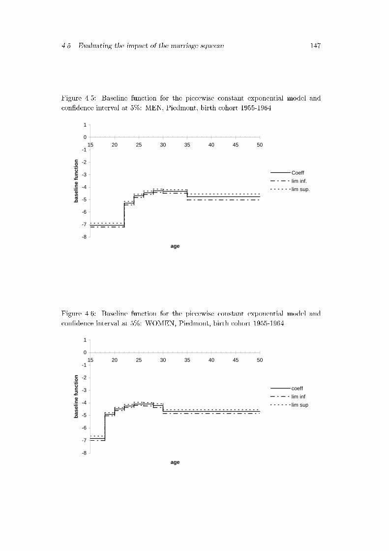
4.5. Evaluating the impact of the marriage squeeze 147
Figure 4.5: Baseline function for the piecewise constant exponential model and
con�dence interval at 5%: MEN, Piedmont, birth cohort 1955-1964
-8
-7
-6
-5
-4
-3
-2
-1
0
1
15 20 25 30 35 40 45 50
age
bas
elin
e fu
nct
ion
Coeff
lim inf.
lim sup.
Figure 4.6: Baseline function for the piecewise constant exponential model and
con�dence interval at 5%: WOMEN, Piedmont, birth cohort 1955-1964
-8
-7
-6
-5
-4
-3
-2
-1
0
1
15 20 25 30 35 40 45 50
age
bas
elin
e fu
nct
ion
coeff
lim inf
lim sup
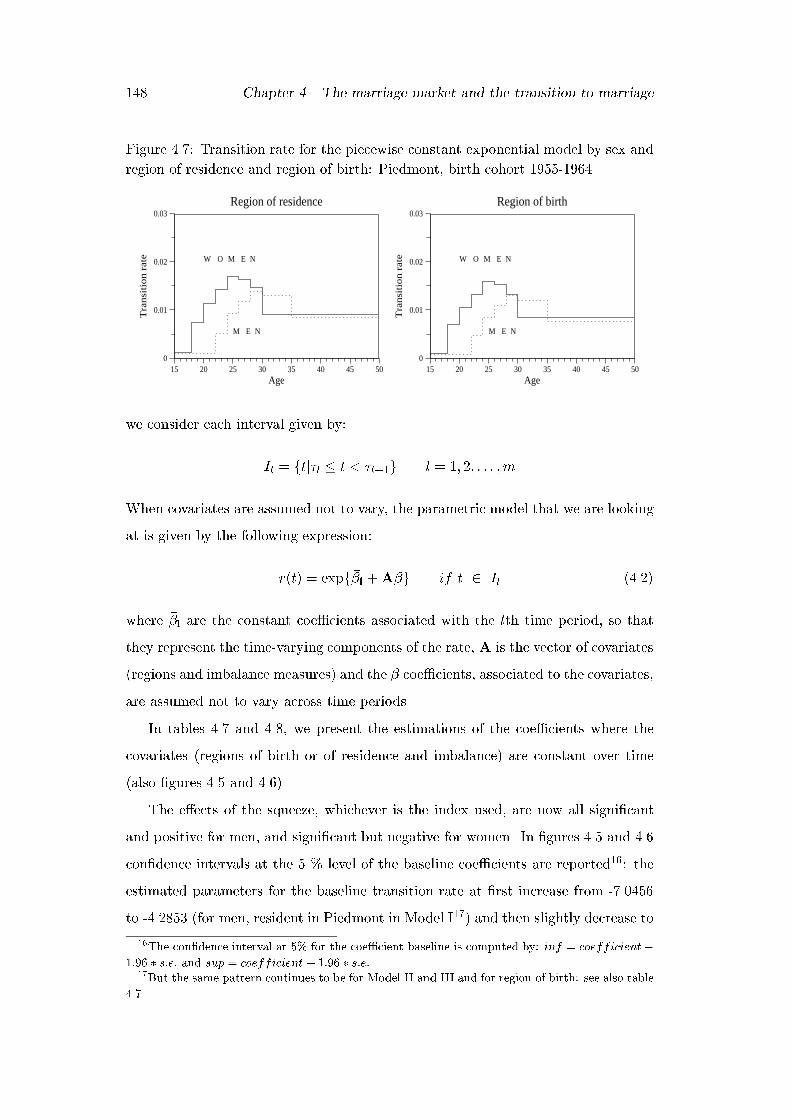
148 Chapter 4. The marriage market and the transition to marriage
Figure 4.7: Transition rate for the piecewise constant exponential model by sex and
region of residence and region of birth: Piedmont, birth cohort 1955-1964
15 20 25 30 35 40 45 500
0.01
0.02
0.03
M E N
W O M E N
Region of residence
Age
Tra
nsi
tion r
ate
15 20 25 30 35 40 45 500
0.01
0.02
0.03
M E N
W O M E N
Region of birth
Age
Tra
nsi
tion r
ate
we consider each interval given by:
Il = ftj�l � t < �l+1g l = 1; 2; : : : ;m
When covariates are assumed not to vary, the parametric model that we are looking
at is given by the following expression:
r(t) = expf��l +A�g if t 2 Il (4.2)
where ��l are the constant coe�cients associated with the lth time period, so that
they represent the time-varying components of the rate, A is the vector of covariates
(regions and imbalance measures) and the � coe�cients, associated to the covariates,
are assumed not to vary across time periods.
In tables 4.7 and 4.8, we present the estimations of the coe�cients where the
covariates (regions of birth or of residence and imbalance) are constant over time
(also �gures 4.5 and 4.6).
The e�ects of the squeeze, whichever is the index used, are now all signi�cant
and positive for men, and signi�cant but negative for women. In �gures 4.5 and 4.6
con�dence intervals at the 5 % level of the baseline coe�cients are reported16: the
estimated parameters for the baseline transition rate at �rst increase from -7.0456
to -4.2853 (for men, resident in Piedmont in Model I17) and then slightly decrease to
16The con�dence interval at 5% for the coe�cient baseline is computed by: inf = coefficient�
1:96 � s:e: and sup = coefficient + 1:96 � s:e:.17But the same pattern continues to be for Model II and III and for region of birth: see also table
4.7.
4.5. Evaluating the impact of the marriage squeeze 149
-4.7826 (after age 35). The same age pattern, increasing �rst and then decreasing,
can be observed for women: note that the age intervals are di�erent in this case.
The piecewise constant approximates the curves of marriage by ages. Therefore,
the transition rate does changes with increasing durations of exposure (�rst marriage
rate varies with age). To the transition rates, constant in each time interval (each
age group), but varying across age-groups (�gure 4.7), one has to add the coe�cient
associated to the set of covariates and assumed not to vary across time periods.
Moreover, it should be stressed that the baselines are non-monotonic for both sexes
and show a di�erent schedule between men and women, slightly anticipated and
higher for the latter, regardless of the region of birth or of residence (�gures 4.5 and
4.6). The transition rates for region of residence and for region of birth (�gure 4.7)
keep the same pattern over time.
The hypothesis regarding the e�ect of the squeeze, regardless of the age pat-
tern, is con�rmed. Men gain from a situation characterised by an imbalance in the
marriage market, by accelerating their transition to �rst marriage, while women ex-
perience a general disadvantage. In particular, an increase in the squeeze (thus an
imbalance against women) has a positive e�ect on the male transition rate, but a
negative e�ect on the female transition rate. In other words, when a squeeze against
women occurs, then men take advantage of the situation having an increasing tran-
sition rate, therefore accelerating their marriage process, while women have greater
di�culties in marrying.
The comparison between nonnested models shows that the model which uses the
squeeze based on the index Ifreq for men (either taking into consideration the region
of birth or the region of residence at the time of the survey) has a BIC statistic
slightly better than the others (even though the di�erences are really low, table 4.7).
For women the model with the lowest BIC is the one which uses Ifreq as imbalance
(table 4.8).
4.5.3 The piecewise constant exponential model with period-speci�c
e�ects
The great advantage of the piecewise constant exponential model is that it also
o�ers the possibility to easily evaluate the period-speci�c e�ects of the covariates
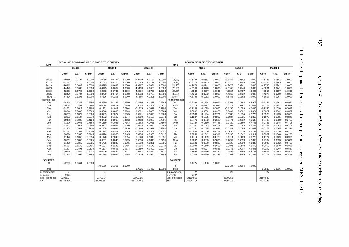
150
Chapter
4.Themarria
gemarket
andthetra
nsitio
nto
marria
ge
Table4.7:Exponentia
lmodelwith
time-p
eriodsbyreg
ion:MEN,ITALY
REGION OF RESIDENCE AT THE TIME OF THE SURVEY REGION OF RESIDENCE AT BIRTHMEN MEN
Coeff S.E. Signif Coeff S.E. Signif Coeff S.E. Signif Coeff S.E. Signif Coeff S.E. Signif Coeff S.E. Signif
[15,22) -7.0456 0.0794 1.0000 -7.0456 0.0794 1.0000 -7.0409 0.0794 1.0000 [15,22) -7.1389 0.0852 1.0000 -7.1389 0.0852 1.0000 -7.1347 0.0852 1.0000[22,24) -5.2843 0.0726 1.0000 -5.2843 0.0726 1.0000 -5.2893 0.0727 1.0000 [22,24) -5.3728 0.0785 1.0000 -5.3728 0.0785 1.0000 -5.3783 0.0785 1.0000[24,26) -4.6915 0.0683 1.0000 -4.6915 0.0683 1.0000 -4.6967 0.0684 1.0000 [24,26) -4.7678 0.0741 1.0000 -4.7678 0.0741 1.0000 -4.7735 0.0742 1.0000[26,28) -4.4445 0.0682 1.0000 -4.4445 0.0682 1.0000 -4.4483 0.0683 1.0000 [26,28) -4.5160 0.0740 1.0000 -4.5160 0.0740 1.0000 -4.5201 0.0741 1.0000[28,30) -4.2853 0.0700 1.0000 -4.2853 0.0700 1.0000 -4.2879 0.0700 1.0000 [28,30) -4.3534 0.0757 1.0000 -4.3534 0.0757 1.0000 -4.3559 0.0757 1.0000[30,35) -4.3479 0.0704 1.0000 -4.3479 0.0704 1.0000 -4.3503 0.0702 1.0000 [30,35) -4.4260 0.0762 1.0000 -4.4260 0.0762 1.0000 -4.4279 0.0760 1.0000[35,+) -4.7826 0.1206 1.0000 -4.7826 0.1206 1.0000 -4.7865 0.1201 1.0000 [35,+) -4.8786 0.1262 1.0000 -4.8786 0.1262 1.0000 -4.8817 0.1257 1.0000
Piedmont (base) Piedmont (base)Vaa -0.4529 0.1381 0.9990 -0.4530 0.1381 0.9990 -0.4496 0.1377 0.9989 Vaa -0.5268 0.1764 0.9972 -0.5268 0.1764 0.9972 -0.5236 0.1761 0.9971Lom 0.0034 0.0808 0.0340 0.0034 0.0808 0.0340 0.0038 0.0807 0.0371 Lom 0.0115 0.0887 0.1027 0.0115 0.0887 0.1027 0.0117 0.0887 0.1048Taa -0.1231 0.1012 0.7764 -0.1231 0.1012 0.7764 -0.1215 0.1011 0.7706 Taa -0.1158 0.1099 0.7080 -0.1158 0.1099 0.7080 -0.1140 0.1098 0.7012Ven -0.0640 0.0893 0.5269 -0.0640 0.0893 0.5269 -0.0631 0.0893 0.5204 Ven 0.0367 0.0962 0.2973 0.0367 0.0962 0.2974 0.0377 0.0962 0.3052Fvg -0.0789 0.1077 0.5366 -0.0789 0.1077 0.5365 -0.0771 0.1076 0.5260 Fvg -0.0988 0.1234 0.5771 -0.0988 0.1234 0.5770 -0.0970 0.1233 0.5685Lig -0.3392 0.1127 0.9974 -0.3392 0.1127 0.9974 -0.3380 0.1127 0.9973 Lig -0.1987 0.1255 0.8867 -0.1987 0.1255 0.8868 -0.1972 0.1255 0.8841Tos -0.0498 0.0909 0.4164 -0.0498 0.0909 0.4163 -0.0488 0.0907 0.4091 Tos 0.0470 0.0982 0.3682 0.0471 0.0982 0.3682 0.0480 0.0980 0.3757Umb -0.1170 0.1086 0.7183 -0.1169 0.1086 0.7183 -0.1162 0.1085 0.7160 Umb -0.0729 0.1150 0.4738 -0.0729 0.1150 0.4738 -0.0723 0.1148 0.4708Er -0.2192 0.0971 0.9760 -0.2192 0.0971 0.9760 -0.2193 0.0970 0.9762 Er -0.2291 0.1053 0.9704 -0.2291 0.1053 0.9704 -0.2291 0.1053 0.9705
Mar -0.1205 0.0981 0.7810 -0.1205 0.0981 0.7810 -0.1240 0.0981 0.7940 Mar -0.0141 0.1065 0.1056 -0.0141 0.1065 0.1057 -0.0179 0.1065 0.1336Laz -0.1791 0.0987 0.9304 -0.1792 0.0987 0.9305 -0.1793 0.0982 0.9321 Laz -0.0898 0.1036 0.6137 -0.0898 0.1036 0.6139 -0.0904 0.1030 0.6200Abr 0.0714 0.0956 0.5445 0.0714 0.0956 0.5445 0.0708 0.0955 0.5412 Abr 0.0936 0.1042 0.6311 0.0936 0.1042 0.6311 0.0929 0.1040 0.6283Mol 0.1470 0.1048 0.8394 0.1470 0.1048 0.8394 0.1528 0.1048 0.8551 Mol 0.1714 0.1109 0.8778 0.1714 0.1109 0.8778 0.1774 0.1109 0.8901Cam 0.0601 0.0845 0.5225 0.0601 0.0845 0.5225 0.0638 0.0845 0.5495 Cam 0.2097 0.0853 0.9860 0.2097 0.0853 0.9860 0.2134 0.0853 0.9876Pug 0.1425 0.0849 0.9065 0.1425 0.0849 0.9065 0.1358 0.0851 0.8895 Pug 0.2120 0.0880 0.9839 0.2120 0.0880 0.9839 0.2046 0.0882 0.9797Bas -0.1054 0.1146 0.6425 -0.1054 0.1146 0.6425 -0.1016 0.1146 0.6249 Bas -0.0390 0.1148 0.2662 -0.0391 0.1148 0.2663 -0.0350 0.1148 0.2398Cal 0.1527 0.0891 0.9134 0.1527 0.0891 0.9134 0.1580 0.0892 0.9237 Cal 0.2245 0.0907 0.9866 0.2245 0.0907 0.9866 0.2299 0.0908 0.9887Sic 0.0546 0.0884 0.4632 0.0546 0.0884 0.4631 0.0382 0.0890 0.3317 Sic 0.1994 0.0896 0.9740 0.1994 0.0896 0.9739 0.1821 0.0903 0.9564Sar -0.1218 0.0994 0.7794 -0.1218 0.0994 0.7795 -0.1209 0.0994 0.7759 Sar 0.0303 0.0999 0.2386 0.0303 0.0999 0.2385 0.0313 0.0999 0.2459
SQUEEZE: SQUEEZE:S 5.2692 1.0661 1.0000 S 5.4725 1.1186 1.0000I 10.5356 2.1315 1.0000 I 10.9424 2.2364 1.0000
Ifreq 8.9895 1.7460 1.0000 Ifreq 9.3538 1.8236 1.0000n. parameters: 27 27 27 n. parameters: 27 27 27n. events 3921 n. events 3787Log -likelihood: -22721.94 -22721.94 -22720.85 Log -likelihood: -21900.56 -21900.56 -21899.33BIC: -15702.570 -15702.573 -15704.752 BIC: -14926.715 -14926.719 -14929.189
Model I Model II Model III Model I Model II Model III
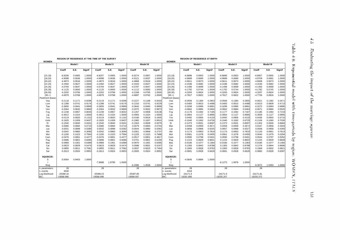
4.5.Evaluatin
gtheim
pact
ofthemarria
gesqueeze
151
Table4.8:Exponentia
lmodelwith
time-p
eriodsbyreg
ion:WOMEN,ITALY
REGION OF RESIDENCE AT THE TIME OF THE SURVEY REGION OF RESIDENCE AT BIRTHWOMEN WOMEN
Coeff S.E. Signif Coeff S.E. Signif Coeff S.E. Signif Coeff S.E. Signif Coeff S.E. Signif Coeff S.E. Signif
[15,18) -6.8206 0.0905 1.0000 -6.8207 0.0905 1.0000 -6.8274 0.0907 1.0000 [15,18) -6.8896 0.0953 1.0000 -6.8896 0.0953 1.0000 -6.8957 0.0955 1.0000[18,20) -4.9098 0.0636 1.0000 -4.9098 0.0636 1.0000 -4.9121 0.0637 1.0000 [18,20) -4.9689 0.0690 1.0000 -4.9689 0.0690 1.0000 -4.9709 0.0691 1.0000[20,22) -4.4873 0.0616 1.0000 -4.4873 0.0616 1.0000 -4.4868 0.0616 1.0000 [20,22) -4.5611 0.0673 1.0000 -4.5611 0.0673 1.0000 -4.5608 0.0673 1.0000[22,24) -4.2450 0.0627 1.0000 -4.2450 0.0627 1.0000 -4.2443 0.0627 1.0000 [22,24) -4.3186 0.0682 1.0000 -4.3186 0.0682 1.0000 -4.3184 0.0682 1.0000[24,26) -4.0794 0.0647 1.0000 -4.0794 0.0647 1.0000 -4.0787 0.0647 1.0000 [24,26) -4.1496 0.0699 1.0000 -4.1496 0.0699 1.0000 -4.1493 0.0699 1.0000[26,28) -4.1125 0.0693 1.0000 -4.1125 0.0693 1.0000 -4.1112 0.0693 1.0000 [26,28) -4.1792 0.0744 1.0000 -4.1792 0.0744 1.0000 -4.1782 0.0745 1.0000[28,30) -4.2202 0.0766 1.0000 -4.2202 0.0766 1.0000 -4.2168 0.0765 1.0000 [28,30) -4.3293 0.0824 1.0000 -4.3293 0.0824 1.0000 -4.3257 0.0824 1.0000[30,+) -4.6979 0.0768 1.0000 -4.6979 0.0768 1.0000 -4.6897 0.0762 1.0000 [30,+) -4.7817 0.0822 1.0000 -4.7817 0.0822 1.0000 -4.7726 0.0816 1.0000
Piedmont (base) Piedmont (base)Vaa -0.2118 0.1171 0.9296 -0.2119 0.1171 0.9296 -0.2227 0.1168 0.9433 Vaa -0.0506 0.1384 0.2853 -0.0506 0.1384 0.2855 -0.0621 0.1382 0.3471Lom -0.1288 0.0741 0.9176 -0.1288 0.0741 0.9176 -0.1310 0.0741 0.9229 Lom -0.0483 0.0810 0.4488 -0.0483 0.0810 0.4488 -0.0510 0.0809 0.4713Taa -0.3655 0.0941 0.9999 -0.3655 0.0941 0.9999 -0.3642 0.0940 0.9999 Taa -0.3299 0.0995 0.9991 -0.3299 0.0995 0.9991 -0.3272 0.0993 0.9990Ven -0.2064 0.0832 0.9869 -0.2064 0.0832 0.9869 -0.2072 0.0832 0.9873 Ven -0.0662 0.0884 0.5464 -0.0662 0.0884 0.5464 -0.0671 0.0884 0.5520Fvg -0.1238 0.0957 0.8040 -0.1239 0.0957 0.8042 -0.1267 0.0958 0.8138 Fvg -0.1176 0.1092 0.7185 -0.1177 0.1092 0.7187 -0.1185 0.1092 0.7219Lig -0.4912 0.1024 1.0000 -0.4912 0.1024 1.0000 -0.4905 0.1024 1.0000 Lig -0.3954 0.1127 0.9995 -0.3954 0.1127 0.9995 -0.3939 0.1127 0.9995Tos -0.0119 0.0820 0.1152 -0.0119 0.0820 0.1152 -0.0166 0.0818 0.1605 Tos 0.0492 0.0905 0.4133 0.0492 0.0905 0.4133 0.0436 0.0903 0.3710Umb -0.1925 0.1009 0.9437 -0.1925 0.1009 0.9437 -0.1982 0.1007 0.9510 Umb -0.1040 0.1062 0.6726 -0.1040 0.1062 0.6725 -0.1106 0.1060 0.7030Er -0.1540 0.0840 0.9331 -0.1540 0.0840 0.9331 -0.1563 0.0839 0.9375 Er -0.1373 0.0931 0.8597 -0.1373 0.0931 0.8597 -0.1402 0.0930 0.8684
Mar 0.0080 0.0894 0.0710 0.0080 0.0894 0.0710 0.0079 0.0894 0.0704 Mar 0.0458 0.0959 0.3671 0.0458 0.0959 0.3672 0.0447 0.0958 0.3593Laz 0.0031 0.0898 0.0280 0.0032 0.0898 0.0282 -0.0044 0.0890 0.0392 Laz 0.0656 0.0968 0.5025 0.0657 0.0968 0.5027 0.0558 0.0958 0.4393Abr 0.0342 0.0860 0.3090 0.0342 0.0860 0.3090 0.0301 0.0858 0.2737 Abr 0.1173 0.0953 0.7819 0.1173 0.0953 0.7819 0.1120 0.0951 0.7613Mol -0.1200 0.1023 0.7594 -0.1200 0.1023 0.7594 -0.1225 0.1023 0.7688 Mol 0.0061 0.1078 0.0455 0.0061 0.1078 0.0455 0.0040 0.1079 0.0294Cam -0.0476 0.0801 0.4477 -0.0476 0.0801 0.4477 -0.0517 0.0801 0.4817 Cam 0.0590 0.0798 0.5401 0.0590 0.0798 0.5401 0.0544 0.0797 0.5052Pug 0.0686 0.0801 0.6085 0.0686 0.0801 0.6086 0.0701 0.0801 0.6190 Pug 0.1224 0.0829 0.8601 0.1224 0.0829 0.8602 0.1225 0.0829 0.8608Bas -0.0969 0.1061 0.6389 -0.0969 0.1061 0.6389 -0.0970 0.1061 0.6395 Bas -0.0185 0.1077 0.1364 -0.0185 0.1077 0.1364 -0.0185 0.1077 0.1365Cal 0.0623 0.0829 0.5475 0.0623 0.0829 0.5474 0.0586 0.0831 0.5197 Cal 0.1305 0.0842 0.8788 0.1305 0.0842 0.8788 0.1276 0.0844 0.8696Sic 0.0855 0.0811 0.7081 0.0855 0.0811 0.7082 0.0937 0.0815 0.7494 Sic 0.1900 0.0828 0.9783 0.1900 0.0828 0.9783 0.1969 0.0832 0.9821Sar -0.2613 0.0924 0.9953 -0.2613 0.0924 0.9953 -0.2605 0.0924 0.9952 Sar -0.0891 0.0928 0.6628 -0.0891 0.0928 0.6628 -0.0883 0.0928 0.6587
SQUEEZE: SQUEEZE:S -3.9354 0.9403 1.0000 S -4.0645 0.9994 1.0000I -7.8688 1.8795 1.0000 I -8.1273 1.9978 1.0000
Ifreq -6.2080 1.4549 1.0000 Ifreq -6.3072 1.5393 1.0000n. parameters: 28 28 28 n. parameters: 28 28 28n. events 4530 n. events 4318Log-likelihood: -25388.16 -25388.15 -25387.85 Log-likelihood: -24171.9 -24171.9 -24171.81BIC: -19588.986 -19588.996 -19589.597 BIC: -18281.895 -18255.207 -18255.372
Model I Model II Model III Model I Model II Model III
152 Chapter 4. The marriage market and the transition to marriage
under study. Once the e�ect of the marriage squeeze has been ascertained, it is
also reasonable to think about its distribution over time. Evidence from previous
studies showed that the e�ect of the squeeze was very likely to act in the sense of a
shift in the timing of marriage, instead of reducing the total amount of people who
accessed to marriage (Schoen, 1983[164]). In particular, third world societies seem
to be sensitive to the marriage squeeze as it can in uence both the rate and the
distribution of marriages. In developed countries, only the distribution of marriages
is sensitive to imbalances in the number of the two sexes: the rate of marriage is
relatively insusceptible to marriage squeezes (Schoen, 1983[164]).
It is now interesting to see whether the imbalance in the marriage market pro-
duces period-speci�c e�ects. A further generalisation of the piecewise constant ex-
ponential model can be obtained if we want also to include the e�ect of the time-
constant covariates in each time interval. As we said before the standard piecewise
constant exponential model requires splitting the time axis. Accordingly, also the
e�ects of the covariates can be computed for each time interval18.
In this case the model assumes the following expression:
r(t) = expf��l +A�lg if t 2 Il (4.3)
where the ��l are, as we said in the previous case, the constant coe�cients associ-
ated with the lth time period, A is the vector of covariates (regions and imbalance
measures) and the �l coe�cients of the covariates are now speci�c for each of the
lth interval.
Our purpose is now to investigate the e�ect of the squeeze by age. By estimating
that, the model provides also the e�ects, for each speci�ed age group, of all covariates
included: in this case we have the regions of residence or the regions of birth. This
implies a considerable increase in the number of parameters to be estimated: in
fact, if we split the time axis into 8 intervals, we have to estimate the baseline e�ect
for each period (8 parameters), the e�ect of the squeeze for each of the intervals
(8 parameters) and the e�ect for each of the 19 regions (because Piedmont is the
reference) for every interval (8x19 parameters). Thus, the number of parameters
18Note that, by introducing constraints which �x the parameters of the covariates to be equal
across time periods we obtain the same result as for the standard exponential model with time
periods (Blossfeld and Rowher, 1995[24]).
4.5. Evaluating the impact of the marriage squeeze 153
to be estimated quickly increases. To follow the principle of parsimony, it would
then be wise to insert some constraints on the parameters of the model to make the
estimation of the remaining ones easier. As our attention is focused on the e�ects of
the squeeze by age, we constrain all other �l parameters referring to regions to be
equal over each time interval19. Several trials have been conducted to optimise the
split of the time interval: for men we then chose a 6-intervals split of the time axis,
while for women we chose 8 di�erent intervals. The results are reported in table 4.9
for men and 4.10 for women. It emerges that for both sexes and either taking into
consideration the region of birth or the region of residence the e�ect of the squeeze
is non-monotonic over the age (see also �gures 4.8, 4.9, 4.10, 4.11).
For men the e�ect of the squeeze is positive and signi�cant for every age and is
particularly high at younger and older ages. Looking at Model II in table 4.9, for
instance, we �nd that the coe�cient of the age pattern of the squeeze e�ect in the
marriage market is positive and very high, 30.9848 before age 23, then it drops to
-0.7147 between age 23 and 25 years (but is not signi�cant), and then rises steadily
to positive values (all signi�cant) up 20.2260 in the age group older than 32 years.
Therefore, for men, there is a clear U-shaped e�ect by age of the imbalance in the
marriage market.
This means that, if the marriage market conditions are bad for women, then
men are advantaged, especially when they are younger than 23 years and when they
are older than, say, 29 (table 4.9 and �gures 4.8 and 4.10). In those age intervals,
they have a high transition rate to marriage, so that the squeeze anticipates (accel-
erates) their transition to �rst marriage. Therefore, a positive squeeze represents
an advantage, with respect to a situation when there is no imbalance, especially for
young men, for which only small information is available. In turn, men older than
25 years pro�t from their relatively smaller uncertainty in the marriage market due
to the fact that they could have built their position in longer time. Apart from
the age group 23-25, from which men seem to su�er a relative disadvantage, but
estimate is not signi�cant, the outcome continues to be the same also if we consider
19However, also models without constraints have been produced to check the goodness of the
estimates of the one without constraints. It emerges that adding constraints for each region improves
the estimates of the e�ects by age of the measure of the squeeze. We do not include the results of
the model without constraints.
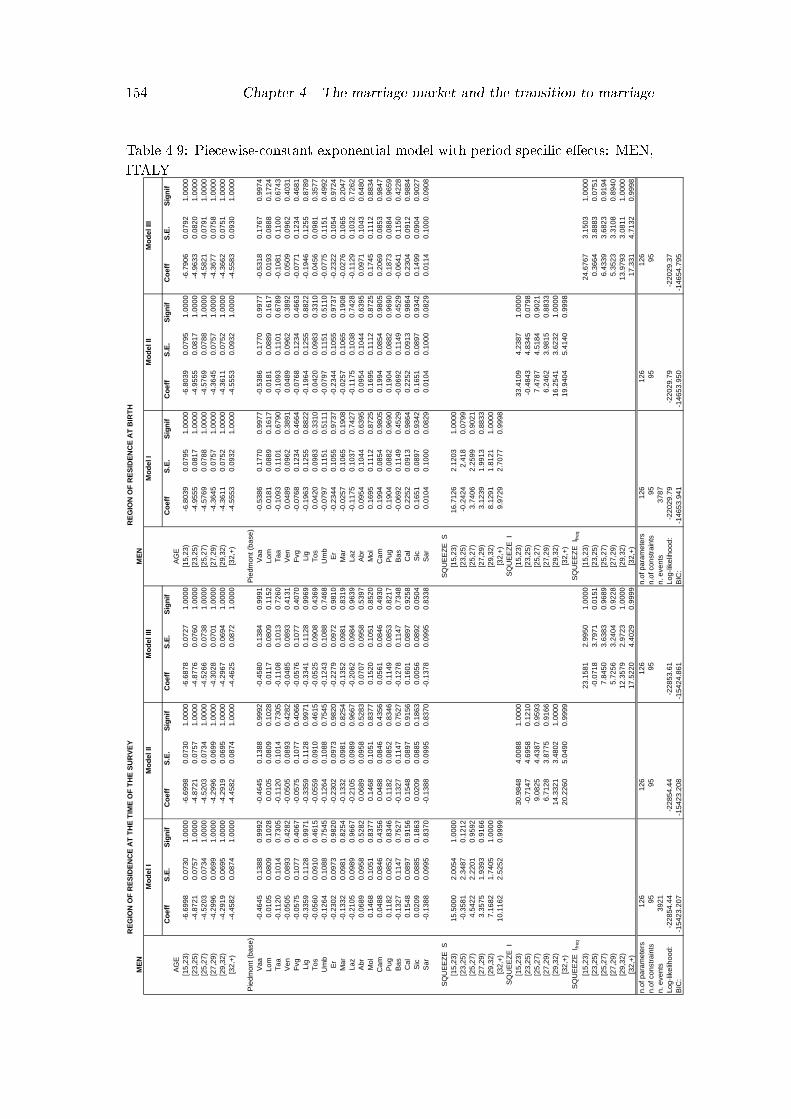
154 Chapter 4. The marriage market and the transition to marriage
Table 4.9: Piecewise-constant exponential model with period speci�c e�ects: MEN,
ITALY
RE
GIO
N O
F R
ES
IDE
NC
E A
T T
HE
TIM
E O
F T
HE
SU
RV
EY
RE
GIO
N O
F R
ES
IDE
NC
E A
T B
IRT
HM
EN
ME
N
Co
eff
S.E
.S
ign
ifC
oef
fS
.E.
Sig
nif
Co
eff
S.E
.S
ign
ifC
oef
fS
.E.
Sig
nif
Co
eff
S.E
.S
ign
ifC
oef
fS
.E.
Sig
nif
AG
EA
GE
[15,
23)
-6.6
998
0.07
301.
0000
-6.6
998
0.07
301.
0000
-6.6
878
0.07
271.
0000
[15,
23)
-6.8
039
0.07
951.
0000
-6.8
039
0.07
951.
0000
-6.7
906
0.07
921.
0000
[23,
25)
-4.8
721
0.07
571.
0000
-4.8
721
0.07
571.
0000
-4.8
776
0.07
601.
0000
[23,
25)
-4.9
555
0.08
171.
0000
-4.9
555
0.08
171.
0000
-4.9
633
0.08
201.
0000
[25,
27)
-4.5
203
0.07
341.
0000
-4.5
203
0.07
341.
0000
-4.5
266
0.07
381.
0000
[25,
27)
-4.5
769
0.07
881.
0000
-4.5
769
0.07
881.
0000
-4.5
821
0.07
911.
0000
[27,
29)
-4.2
996
0.06
991.
0000
-4.2
996
0.06
991.
0000
-4.3
028
0.07
011.
0000
[27,
29)
-4.3
645
0.07
571.
0000
-4.3
645
0.07
571.
0000
-4.3
677
0.07
581.
0000
[29,
32)
-4.2
919
0.06
951.
0000
-4.2
919
0.06
951.
0000
-4.2
967
0.06
941.
0000
[29,
32)
-4.3
611
0.07
521.
0000
-4.3
611
0.07
521.
0000
-4.3
662
0.07
511.
0000
[32,
+)
-4.4
582
0.08
741.
0000
-4.4
582
0.08
741.
0000
-4.4
625
0.08
721.
0000
[32,
+)
-4.5
553
0.09
321.
0000
-4.5
553
0.09
321.
0000
-4.5
583
0.09
301.
0000
Pie
dmon
t (ba
se)
Pie
dmon
t (ba
se)
Vaa
-0.4
645
0.13
880.
9992
-0.4
645
0.13
880.
9992
-0.4
580
0.13
840.
9991
Vaa
-0.5
386
0.17
700.
9977
-0.5
386
0.17
700.
9977
-0.5
318
0.17
670.
9974
Lom
0.01
050.
0809
0.10
280.
0105
0.08
090.
1028
0.01
170.
0809
0.11
52Lo
m0.
0181
0.08
890.
1617
0.01
810.
0889
0.16
170.
0193
0.08
880.
1724
Taa
-0.1
120
0.10
140.
7305
-0.1
120
0.10
140.
7305
-0.1
108
0.10
130.
7260
Taa
-0.1
093
0.11
010.
6790
-0.1
093
0.11
010.
6789
-0.1
081
0.11
000.
6743
Ven
-0.0
505
0.08
930.
4282
-0.0
505
0.08
930.
4282
-0.0
485
0.08
930.
4131
Ven
0.04
890.
0962
0.38
910.
0489
0.09
620.
3892
0.05
090.
0962
0.40
31F
vg-0
.057
50.
1077
0.40
67-0
.057
50.
1077
0.40
66-0
.057
60.
1077
0.40
70F
vg-0
.076
80.
1234
0.46
64-0
.076
80.
1234
0.46
63-0
.077
10.
1234
0.46
81Li
g-0
.335
90.
1128
0.99
71-0
.335
90.
1128
0.99
71-0
.334
10.
1128
0.99
69Li
g-0
.196
30.
1255
0.88
22-0
.196
40.
1255
0.88
22-0
.194
60.
1255
0.87
89T
os-0
.056
00.
0910
0.46
15-0
.055
90.
0910
0.46
15-0
.052
50.
0908
0.43
69T
os0.
0420
0.09
830.
3310
0.04
200.
0983
0.33
100.
0456
0.09
810.
3577
Um
b-0
.126
40.
1088
0.75
45-0
.126
40.
1088
0.75
45-0
.124
30.
1088
0.74
68U
mb
-0.0
797
0.11
510.
5111
-0.0
797
0.11
510.
5110
-0.0
775
0.11
510.
4992
Er
-0.2
302
0.09
730.
9820
-0.2
302
0.09
730.
9820
-0.2
279
0.09
720.
9810
Er
-0.2
344
0.10
550.
9737
-0.2
344
0.10
550.
9737
-0.2
322
0.10
540.
9724
Mar
-0.1
332
0.09
810.
8254
-0.1
332
0.09
810.
8254
-0.1
352
0.09
810.
8319
Mar
-0.0
257
0.10
650.
1908
-0.0
257
0.10
650.
1908
-0.0
276
0.10
650.
2047
Laz
-0.2
105
0.09
890.
9667
-0.2
105
0.09
890.
9667
-0.2
062
0.09
840.
9639
Laz
-0.1
175
0.10
370.
7427
-0.1
175
0.10
380.
7428
-0.1
129
0.10
320.
7262
Abr
0.06
890.
0958
0.52
820.
0689
0.09
580.
5283
0.07
070.
0958
0.53
97A
br0.
0954
0.10
440.
6395
0.09
540.
1044
0.63
950.
0971
0.10
430.
6480
Mol
0.14
680.
1051
0.83
770.
1468
0.10
510.
8377
0.15
200.
1051
0.85
20M
ol0.
1695
0.11
120.
8725
0.16
950.
1112
0.87
250.
1745
0.11
120.
8834
Cam
0.04
880.
0846
0.43
560.
0488
0.08
460.
4356
0.05
610.
0846
0.49
30C
am0.
1994
0.08
540.
9805
0.19
940.
0854
0.98
050.
2069
0.08
530.
9847
Pug
0.11
820.
0852
0.83
460.
1182
0.08
520.
8346
0.11
490.
0853
0.82
17P
ug0.
1904
0.08
820.
9690
0.19
040.
0882
0.96
900.
1873
0.08
840.
9659
Bas
-0.1
327
0.11
470.
7527
-0.1
327
0.11
470.
7527
-0.1
278
0.11
470.
7348
Bas
-0.0
692
0.11
490.
4529
-0.0
692
0.11
490.
4529
-0.0
641
0.11
500.
4228
Cal
0.15
480.
0897
0.91
560.
1548
0.08
970.
9156
0.16
010.
0897
0.92
58C
al0.
2252
0.09
130.
9864
0.22
520.
0913
0.98
640.
2304
0.09
120.
9884
Sic
0.02
090.
0885
0.18
630.
0209
0.08
850.
1863
0.00
560.
0892
0.05
04S
ic0.
1651
0.08
970.
9342
0.16
510.
0897
0.93
420.
1499
0.09
040.
9027
Sar
-0.1
388
0.09
950.
8370
-0.1
388
0.09
950.
8370
-0.1
378
0.09
950.
8338
Sar
0.01
040.
1000
0.08
290.
0104
0.10
000.
0829
0.01
140.
1000
0.09
08
SQ
UE
EZ
E S
SQ
UE
EZ
E S
[15,
23)
15.5
000
2.00
541.
0000
[15,
23)
16.7
126
2.12
031.
0000
[23,
25)
-0.3
581
2.34
870.
1212
[23,
25)
-0.2
424
2.41
80.
0799
[25,
27)
4.54
222.
2201
0.95
92[2
5,27
)3.
7406
2.25
990.
9021
[27,
29)
3.35
751.
9393
0.91
66[2
7,29
)3.
1239
1.99
130.
8833
[29,
32)
7.16
821.
7405
1.00
00[2
9,32
)8.
1291
1.81
211.
0000
[32,
+)
10.1
162
2.52
520.
9999
[32,
+)
9.97
292.
7077
0.99
98S
QU
EE
ZE
I
SQ
UE
EZ
E I
[15,
23)
30.9
848
4.00
881.
0000
[15,
23)
33.4
109
4.23
871.
0000
[23,
25)
-0.7
147
4.69
580.
1210
[23,
25)
-0.4
843
4.83
450.
0798
[25,
27)
9.08
254.
4387
0.95
93[2
5,27
)7.
4787
4.51
840.
9021
[27,
29)
6.71
283.
8775
0.91
66[2
7,29
)6.
2462
3.98
150.
8833
[29,
32)
14.3
321
3.48
021.
0000
[29,
32)
16.2
541
3.62
321.
0000
[32,
+)
20.2
260
5.04
900.
9999
[32,
+)
19.9
404
5.41
400.
9998
SQ
UE
EZ
E I fr
eqS
QU
EE
ZE
I fr
eq
[15,
23)
23.1
581
2.99
501.
0000
[15,
23)
24.6
767
3.15
031.
0000
[23,
25)
-0.0
718
3.79
710.
0151
[23,
25)
0.36
643.
8883
0.07
51[2
5,27
)7.
8450
3.63
830.
9689
[25,
27)
6.43
393.
6823
0.91
94[2
7,29
)5.
7256
3.24
040.
9228
[27,
29)
5.35
233.
3108
0.89
40[2
9,32
)12
.357
92.
9723
1.00
00[2
9,32
)13
.979
33.
0811
1.00
00[3
2,+
)17
.522
04.
4029
0.99
99[3
2,+
)17
.331
4.71
320.
9998
n.of
par
amet
ers
126
126
126
n.of
par
amet
ers
126
126
126
n.of
con
stra
ints
9595
95n.
of c
onst
rain
ts95
9595
n. e
vent
s39
21n.
eve
nts
3787
Log-
likel
ihoo
d:-2
2854
.44
-228
54.4
4-2
2853
.61
Log-
likel
ihoo
d:-2
2029
.79
-220
29.7
9-2
2029
.37
BIC
:-1
5423
.207
-154
23.2
08-1
5424
.861
BIC
:-1
4653
.941
-146
53.9
50-1
4654
.795
Mo
del
IM
od
el II
Mo
del
III
Mo
del
IM
od
el II
Mo
del
III
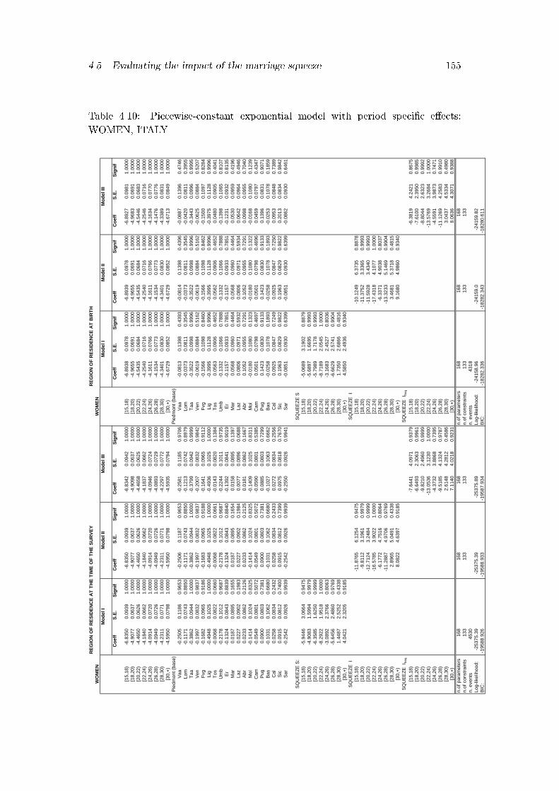
4.5. Evaluating the impact of the marriage squeeze 155
Table 4.10: Piecewise-constant exponential model with period speci�c e�ects:
WOMEN, ITALY
RE
GIO
N O
F R
ES
IDE
NC
E A
T T
HE
TIM
E O
F T
HE
SU
RV
EY
RE
GIO
N O
F R
ES
IDE
NC
E A
T B
IRT
HW
OM
EN
WO
ME
N
Co
eff
S.E
.S
ign
ifC
oef
fS
.E.
Sig
nif
Co
eff
S.E
.S
ign
ifC
oef
fS
.E.
Sig
nif
Co
eff
S.E
.S
ign
ifC
oef
fS
.E.
Sig
nif
[15,
18)
-6.8
350
0.09
391.
0000
-6.8
350
0.09
391.
0000
-6.8
342
0.09
421.
0000
[15,
18)
-6.8
938
0.09
781.
0000
-6.8
939
0.09
781.
0000
-6.8
927
0.09
811.
0000
[18,
20)
-4.9
077
0.06
371.
0000
-4.9
077
0.06
371.
0000
-4.9
098
0.06
371.
0000
[18,
20)
-4.9
655
0.06
911.
0000
-4.9
655
0.06
911.
0000
-4.9
683
0.06
911.
0000
[20,
22)
-4.4
650
0.06
261.
0000
-4.4
650
0.06
261.
0000
-4.4
658
0.06
251.
0000
[20,
22)
-4.5
435
0.06
841.
0000
-4.5
435
0.06
841.
0000
-4.5
446
0.06
831.
0000
[22,
24)
-4.1
840
0.06
621.
0000
-4.1
840
0.06
621.
0000
-4.1
837
0.06
621.
0000
[22,
24)
-4.2
540
0.07
161.
0000
-4.2
540
0.07
161.
0000
-4.2
546
0.07
161.
0000
[24,
26)
-4.0
914
0.07
201.
0000
-4.0
914
0.07
201.
0000
-4.0
946
0.07
241.
0000
[24,
26)
-4.1
611
0.07
661.
0000
-4.1
611
0.07
661.
0000
-4.1
634
0.07
701.
0000
[26,
28)
-4.0
949
0.07
261.
0000
-4.0
949
0.07
261.
0000
-4.0
893
0.07
291.
0000
[26,
28)
-4.1
534
0.07
731.
0000
-4.1
534
0.07
731.
0000
-4.1
476
0.07
761.
0000
[28,
30)
-4.2
311
0.07
711.
0000
-4.2
311
0.07
711.
0000
-4.2
297
0.07
721.
0000
[28,
30)
-4.3
401
0.08
301.
0000
-4.3
401
0.08
301.
0000
-4.3
389
0.08
311.
0000
[30,
+)-4
.595
00.
0798
1.00
00-4
.595
00.
0798
1.00
00-4
.593
50.
0794
1.00
00[3
0,+)
-4.6
729
0.08
521.
0000
-4.6
729
0.08
521.
0000
-4.6
713
0.08
491.
0000
Pie
dmon
t (b
ase)
Pie
dmon
t (ba
se)
Vaa
-0.2
505
0.11
860.
9653
-0.2
506
0.11
870.
9653
-0.2
581
0.11
850.
9706
Vaa
-0.0
813
0.13
980.
4393
-0.0
814
0.13
980.
4396
-0.0
887
0.13
960.
4746
Lom
-0.1
171
0.07
430.
8850
-0.1
171
0.07
430.
8850
-0.1
213
0.07
420.
8979
Lom
-0.0
373
0.08
110.
3545
-0.0
373
0.08
110.
3545
-0.0
420
0.08
110.
3955
Taa
-0.3
862
0.09
441.
0000
-0.3
862
0.09
441.
0000
-0.3
799
0.09
420.
9999
Taa
-0.3
522
0.09
980.
9996
-0.3
522
0.09
980.
9996
-0.3
443
0.09
960.
9995
Ven
-0.1
997
0.08
320.
9837
-0.1
997
0.08
320.
9837
-0.2
007
0.08
320.
9842
Ven
-0.0
619
0.08
840.
5162
-0.0
619
0.08
840.
5162
-0.0
625
0.08
840.
5207
Fvg
-0.1
682
0.09
650.
9186
-0.1
683
0.09
650.
9188
-0.1
641
0.09
650.
9112
Fvg
-0.1
566
0.10
980.
8460
-0.1
566
0.10
980.
8462
-0.1
500
0.10
970.
8284
Lig
-0.4
948
0.10
251.
0000
-0.4
948
0.10
251.
0000
-0.4
936
0.10
251.
0000
Lig
-0.3
995
0.11
280.
9996
-0.3
995
0.11
280.
9996
-0.3
975
0.11
280.
9996
Tos
-0.0
068
0.08
220.
0660
-0.0
068
0.08
220.
0661
-0.0
143
0.08
200.
1384
Tos
0.05
630.
0906
0.46
520.
0562
0.09
060.
4652
0.04
800.
0905
0.40
41U
mb
-0.2
178
0.10
120.
9687
-0.2
178
0.10
120.
9687
-0.2
244
0.10
110.
9735
Um
b-0
.133
20.
1066
0.78
88-0
.133
20.
1066
0.78
88-0
.139
80.
1065
0.81
07E
r-0
.132
40.
0843
0.88
39-0
.132
40.
0843
0.88
40-0
.139
20.
0841
0.90
19E
r-0
.115
70.
0933
0.78
51-0
.115
70.
0933
0.78
51-0
.123
10.
0932
0.81
35M
ar0.
0187
0.08
950.
1655
0.01
870.
0895
0.16
540.
0158
0.08
950.
1397
Mar
0.05
680.
0960
0.44
640.
0568
0.09
600.
4464
0.05
300.
0959
0.41
96La
z0.
0227
0.09
020.
1983
0.02
270.
0902
0.19
840.
0077
0.08
960.
0688
Laz
0.08
060.
0971
0.59
320.
0806
0.09
710.
5934
0.06
420.
0964
0.49
46A
br0.
0233
0.08
620.
2126
0.02
330.
0862
0.21
250.
0181
0.08
620.
1667
Abr
0.10
520.
0955
0.72
910.
1052
0.09
550.
7291
0.09
980.
0955
0.70
40M
ol-0
.141
40.
1024
0.83
25-0
.141
40.
1024
0.83
25-0
.140
90.
1025
0.83
11M
ol-0
.018
00.
1080
0.13
23-0
.018
00.
1080
0.13
22-0
.016
80.
1080
0.12
39C
am-0
.054
90.
0801
0.50
72-0
.054
90.
0801
0.50
72-0
.059
00.
0801
0.53
85C
am0.
0501
0.07
980.
4697
0.05
010.
0798
0.46
960.
0459
0.07
970.
4347
Pug
0.09
000.
0803
0.73
810.
0900
0.08
030.
7381
0.08
850.
0803
0.72
99P
ug0.
1423
0.08
300.
9133
0.14
230.
0830
0.91
330.
1396
0.08
310.
9071
Bas
-0.1
031
0.10
620.
6680
-0.1
031
0.10
620.
6680
-0.1
027
0.10
630.
6662
Bas
-0.0
258
0.10
780.
1893
-0.0
258
0.10
780.
1893
-0.0
253
0.10
780.
1859
Cal
0.02
580.
0834
0.24
320.
0258
0.08
340.
2433
0.02
720.
0834
0.25
56C
al0.
0925
0.08
470.
7249
0.09
250.
0847
0.72
500.
0953
0.08
480.
7389
Sic
0.09
150.
0812
0.74
000.
0915
0.08
120.
7399
0.09
750.
0818
0.76
70S
ic0.
1963
0.08
290.
9822
0.19
630.
0829
0.98
220.
2013
0.08
340.
9842
Sar
-0.2
542
0.09
260.
9939
-0.2
542
0.09
260.
9939
-0.2
550
0.09
260.
9941
Sar
-0.0
851
0.09
300.
6399
-0.0
851
0.09
300.
6399
-0.0
862
0.09
300.
6461
SQ
UE
EZ
E S
:S
QU
EE
ZE
S[1
5,18
)-5
.944
63.
0664
0.94
75[1
5,18
)-5
.068
93.
1902
0.88
79[1
8,20
)-4
.908
31.
5994
0.99
79[1
8,20
)-5
.689
71.
6695
0.99
93[2
0,22
)-6
.358
51.
6250
0.99
99[2
0,22
)-5
.798
91.
7178
0.99
93[2
2,24
)-8
.292
21.
9518
1.00
00[2
2,24
)-8
.718
92.
0545
1.00
00[2
4,26
)-3
.089
22.
3766
0.80
63[2
4,26
)-3
.168
32.
4527
0.80
36[2
6,28
)-5
.645
62.
4860
0.97
69[2
6,28
)-6
.662
92.
5741
0.99
04[2
8,30
)1.
4487
2.52
520.
4338
[28,
30)
1.73
502.
6866
0.48
16[3
0,+)
4.04
212.
3205
0.91
85[3
0,+)
4.58
502.
4936
0.93
40S
QU
EE
ZE
I
SQ
UE
EZ
E
I[1
5,18
)-1
1.87
656.
1254
0.94
75[1
5,18
)-1
0.12
496.
3735
0.88
78[1
8,20
)-9
.811
23.
1961
0.99
79[1
8,20
)-1
1.37
523.
3365
0.99
93[2
0,22
)-1
2.71
243.
2484
0.99
99[2
0,22
)-1
1.59
283.
4340
0.99
93[2
2,24
)-1
6.57
853.
9022
1.00
00[2
2,24
)-1
7.43
184.
1077
1.00
00[2
4,26
)-6
.177
24.
7516
0.80
64[2
4,26
)-6
.337
14.
9038
0.80
37[2
6,28
)-1
1.28
874.
9706
0.97
69[2
6,28
)-1
3.32
335.
1469
0.99
04[2
8,30
)2.
8965
5.04
910.
4338
[28,
30)
3.46
815.
3718
0.48
15[3
0,+)
8.08
224.
6397
0.91
85[3
0,+)
9.16
804.
9860
0.93
40S
QU
EE
ZE
I fr
eqS
QU
EE
ZE
I fr
eq
[15,
18)
-7.6
441
4.09
710.
9379
[15,
18)
-6.3
819
4.24
210.
8675
[18,
20)
-6.6
493
2.30
630.
9961
[18,
20)
-7.6
100
2.39
500.
9985
[20,
22)
-9.8
210
2.49
600.
9999
[20,
22)
-8.8
044
2.63
230.
9992
[22,
24)
-13.
0536
3.12
301.
0000
[22,
24)
-13.
5769
3.26
841.
0000
[24,
26)
-4.3
732
3.88
680.
7395
[24,
26)
-4.5
591
3.98
730.
7471
[26,
28)
-9.5
185
4.13
240.
9787
[26,
28)
-11.
1269
4.25
830.
9910
[28,
30)
2.61
484.
2812
0.45
86[2
8,30
)3.
0437
4.53
340.
4980
[30,
+)7.
1140
4.02
180.
9231
[30,
+)8.
0636
4.30
710.
9388
n.of
par
amet
ers
168
168
168
n.of
par
amet
ers
168
168
168
n.of
con
stra
ints
133
133
133
n.of
con
stra
ints
133
133
133
n. e
vent
s45
30n.
eve
nts
4318
Log-
likel
ihoo
d:-2
5375
.39
-253
75.3
9-2
5375
.89
Log-
likel
ihoo
d:-2
4158
.96
-241
59.0
-241
59.8
2B
IC:
-195
88.9
26-1
9588
.933
-195
87.9
34B
IC:
-182
82.3
36-1
8282
.343
-182
80.6
11
Mo
del
IM
od
el II
Mo
del
III
Mo
del
IM
od
el II
Mo
del
III
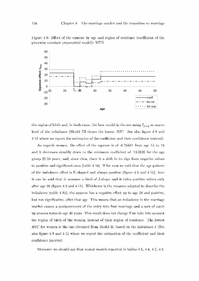
156 Chapter 4. The marriage market and the transition to marriage
Figure 4.8: E�ect of the squeeze by age and region of residence (coe�cient of the
piecewise constant exponential model): MEN
-30
-20
-10
0
10
20
30
40
50
60
15 20 25 30 35 40 45 50
age
Sq
uee
ze e
ffec
t: I f
req
coeff
lim inf
lim sup
the region of birth and, in both cases, the best model is the one using Ifreq as macro
level of the imbalance (Model III shows the lowest BIC. See also �gure 4.8 and
4.10 where we report the estimation of the coe�cient and their con�dence interval).
As regards women, the e�ect of the squeeze is of -0.76441 from age 15 to 18
and it decreases steadily down to the minimum coe�cient of -13.0536 for the age
group 22-24 years, and, since then, there is a shift in its sign from negative values
to positive and signi�cant ones (table 4.10). If for men we said that the age pattern
of the imbalance e�ect is U-shaped and always positive (�gure 4.8 and 4.10), here
it can be said that it assumes a kind of J-shape and it takes positive values only
after age 28 (�gure 4.9 and 4.11). Whichever is the measure adopted to describe the
imbalance (table 4.10), the squeeze has a negative e�ect up to age 28 and positive,
but not signi�cative, after that age. This means that an imbalance in the marriage
market causes a postponement of the entry into �rst marriage and a sort of catch
up process towards age 30 years. This result does not change if we take into account
the region of birth of the women, instead of their region of residence. The lowest
BIC for women is the one obtained from Model II, based on the imbalance I (See
also �gure 4.9 and 4.11 where we report the estimation of the coe�cient and their
con�dence interval).
Moreover we should say that nested models reported in tables 4.5, 4.6, 4.7, 4.8,
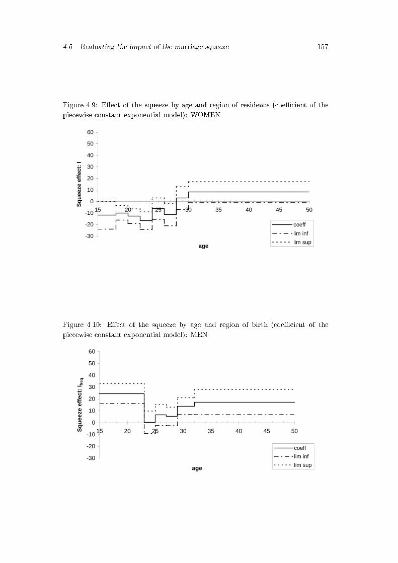
4.5. Evaluating the impact of the marriage squeeze 157
Figure 4.9: E�ect of the squeeze by age and region of residence (coe�cient of the
piecewise constant exponential model): WOMEN
-30
-20
-10
0
10
20
30
40
50
60
15 20 25 30 35 40 45 50
age
Sq
uee
ze e
ffec
t: I
coeff
lim inf
lim sup
Figure 4.10: E�ect of the squeeze by age and region of birth (coe�cient of the
piecewise constant exponential model): MEN
lim inf lim sup-30
-20
-10
0
10
20
30
40
50
60
15 20 25 30 35 40 45 50
age
Sq
uee
ze e
ffec
t: I f
req
coeff
lim inf
lim sup

158 Chapter 4. The marriage market and the transition to marriage
Figure 4.11: E�ect of the squeeze by age and region of birth (coe�cient of the
piecewise constant exponential model): WOMEN
-30
-20
-10
0
10
20
30
40
50
60
15 20 25 30 35 40 45 50
age
Sq
uee
ze e
ffec
t: I
coeff
lim inf
lim sup
4.9, 4.10 have been compared separately for men and women, for region of birth
and of residence. In table 4.11, log-likelihood, number of parameters, constraints
and events of every model are reported. In the second part only nested models
are compared by means of the log-likelihood ratio. By looking at the log-likelihood
ratio, an improvement of the models with �ner speci�cation of the rate emerges.
However, models A II, A III and A IV compared to the model A I (without the
e�ect of the squeeze), do show an improvement for women (p-value=0.000), whereas
for men they do not work well: but this is understandable, given that, for men, the
e�ect of the squeeze obtained by applying the Cox model was not signi�cant. Also,
moving from the proportional hazards models to the piecewise constant ones, there
is a sensitive improvement in the log-likelihood ratio: this means that the piecewise
constant exponential model, which includes the parameters referred to each of the
sub-intervals, succeeds in representing the non-monotonicity of the process (therefore
we refuse the null hypothesis according to which the exceeding parameters are not
statistically signi�cant). The same occurs comparing the models in tables 4.9 and
4.10 to the one without period e�ect of the squeeze (tables 4.7 and 4.8). It should
also be noted that some trials have been conducted to see what happens including
the indicators of the squeeze referring to the region of birth and to the region of
residence. For most of the individuals region of birth an region of residence will
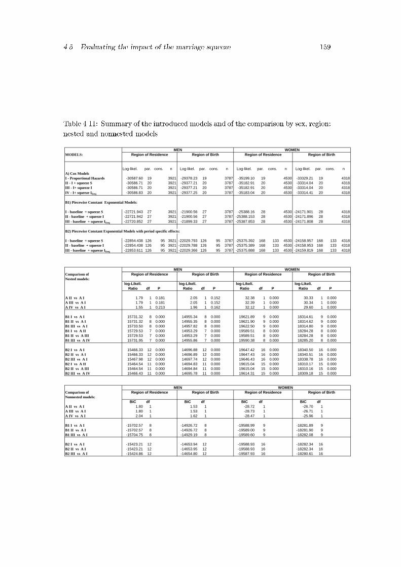
4.5. Evaluating the impact of the marriage squeeze 159
Table 4.11: Summary of the introduced models and of the comparison by sex, region:
nested and nonnested models
MODELS:
Log-likel. par. cons. n Log-likel. par. cons. n Log-likel. par. cons. n Log-likel. par. cons. nA) Cox ModelsI - Proportional Hazards -30587.60 19 3921 -29378.23 19 3787 -35199.10 19 4530 -33329.21 19 4318II - I + squeeze S -30586.71 20 3921 -29377.21 20 3787 -35182.91 20 4530 -33314.04 20 4318III - I+ squeeze I -30586.71 20 3921 -29377.21 20 3787 -35182.91 20 4530 -33314.04 20 4318IV - I+ squeeze Ifreq -30586.83 20 3921 -29377.25 20 3787 -35183.04 20 4530 -33314.41 20 4318
B1) Piecewise Constant Exponential Models:
I - baseline + squeeze S -22721.943 27 3921 -21900.56 27 3787 -25388.16 28 4530 -24171.901 28 4318II - baseline + squeeze I -22721.942 27 3921 -21900.56 27 3787 -25388.153 28 4530 -24171.896 28 4318III - baseline + squeeze Ifreq -22720.852 27 3921 -21899.33 27 3787 -25387.853 28 4530 -24171.808 28 4318
B2) Piecewise Constant Exponential Models with period specific effects:
I - baseline + squeeze S -22854.438 126 95 3921 -22029.793 126 95 3787 -25375.392 168 133 4530 -24158.957 168 133 4318II - baseline + squeeze I -22854.438 126 95 3921 -22029.788 126 95 3787 -25375.389 168 133 4530 -24158.953 168 133 4318III - baseline + squeeze Ifreq -22853.611 126 95 3921 -22029.366 126 95 3787 -25375.888 168 133 4530 -24159.819 168 133 4318
Comparison of Nested models:
log-Likeli. log-Likeli. log-Likeli. log-Likeli.Ratio df P Ratio df P Ratio df P Ratio df P
A II vs A I 1.79 1 0.181 2.05 1 0.152 32.38 1 0.000 30.33 1 0.000A III vs A I 1.79 1 0.181 2.05 1 0.152 32.39 1 0.000 30.34 1 0.000A IV vs A I 1.55 1 0.213 1.96 1 0.162 32.12 1 0.000 29.60 1 0.000
B1 I vs A I 15731.32 8 0.000 14955.34 8 0.000 19621.89 9 0.000 18314.61 9 0.000B1 II vs A I 15731.32 8 0.000 14955.35 8 0.000 19621.90 9 0.000 18314.62 9 0.000B1 III vs A I 15733.50 8 0.000 14957.82 8 0.000 19622.50 9 0.000 18314.80 9 0.000B1 I vs A II 15729.53 7 0.000 14953.29 7 0.000 19589.51 8 0.000 18284.28 8 0.000B1 II vs A III 15729.53 7 0.000 14953.29 7 0.000 19589.51 8 0.000 18284.28 8 0.000B1 III vs A IV 15731.95 7 0.000 14955.86 7 0.000 19590.38 8 0.000 18285.20 8 0.000
B2 I vs A I 15466.33 12 0.000 14696.88 12 0.000 19647.42 16 0.000 18340.50 16 0.000B2 II vs A I 15466.33 12 0.000 14696.89 12 0.000 19647.43 16 0.000 18340.51 16 0.000B2 III vs A I 15467.98 12 0.000 14697.74 12 0.000 19646.43 16 0.000 18338.78 16 0.000B2 I vs A II 15464.54 11 0.000 14694.83 11 0.000 19615.04 15 0.000 18310.17 15 0.000B2 II vs A III 15464.54 11 0.000 14694.84 11 0.000 19615.04 15 0.000 18310.16 15 0.000B2 III vs A IV 15466.43 11 0.000 14695.78 11 0.000 19614.31 15 0.000 18309.18 15 0.000
Comparison of Nonnested models:
BIC df BIC df BIC df BIC dfA II vs A I 1.80 1 1.53 1 -28.72 1 -26.70 1A III vs A I 1.80 1 1.53 1 -28.73 1 -26.71 1A IV vs A I 2.04 1 1.62 1 -28.47 1 -25.96 1
B1 I vs A I -15702.57 8 -14926.72 8 -19588.99 9 -18281.89 9B1 II vs A I -15702.57 8 -14926.72 8 -19589.00 9 -18281.90 9B1 III vs A I -15704.75 8 -14929.19 8 -19589.60 9 -18282.08 9
B2 I vs A I -15423.21 12 -14653.94 12 -19588.93 16 -18282.34 16B2 II vs A I -15423.21 12 -14653.95 12 -19588.93 16 -18282.34 16B2 III vs A I -15424.86 12 -14654.80 12 -19587.93 16 -18280.61 16
Region of Birth
Region of Residence Region of Birth Region of Residence Region of Birth
Region of Birth Region of ResidenceRegion of Residence
MEN WOMEN
WOMENRegion of Birth
MEN WOMEN
MEN
Region of ResidenceRegion of Residence Region of Birth
160 Chapter 4. The marriage market and the transition to marriage
coincide and this can bring about problems in the estimations of the parameters.
The inclusion of both indicators does not improve the models: the e�ects are not
signi�cant, neither for women nor for men, although their signs are positive for
men and negative for women, con�rming the previous models. Cox and piecewise
constant exponential models where we include both region of birth and region of
residence are reported in the appendix.
Some concluding remarks for the comparison between the piecewise constant
exponential rate model and the semi-parametric model of Cox regression can be
reminded: both of them are proportional hazards models. The di�erence is due to
the fact that the Cox model leaves the baseline hazard rate completely unspeci�ed,
while the piecewise constant model tries to approximate it with a series of period-
speci�c constants. It is worth noting that, with an increasing number of intervals
of decreasing width of time periods, a piecewise constant model basically becomes
a Cox model providing direct estimation of the baseline hazard rate (Blossfeld and
Rowher, 1995[24]). The advantage of using the piecewise constant model instead of
the Cox model is that it o�ers direct estimates of the baseline rate.
4.6 Marriage squeeze and other determinants of the
transition to marriage
Up to now, the role of compositional constraints in the process of transition to
�rst marriage has been analysed without considering other characteristics of the
individual life-courses. What is now interesting is to see whether including other
covariates, regarding birth cohort, region of birth, employment and education, makes
the e�ects of the imbalance on the marriage market disappearing. The models we
are going to introduce, take into account the following explanatory variables for each
sex:
- marriage market: continuous time-varying covariate;
- birth cohort: 1955 � 1959; 1960 � 1964; 1965 � 1969; >= 1970 time independent;
- region of birth: time independent;
- educational attainment: time independent;
4.6. Marriage squeeze and other determinants of the transition to marriage 161
- �rst job: time-varying covariate;
As macro variable for the marriage opportunities we include squeeze measures, which
preliminarily showed an age dependent e�ect on both men and women. In the �rst
part of this chapter, the descriptive analysis of the transition to �rst marriage by
birth cohort showed that there has been a changing pattern in the marital behaviour
of Italian cohorts for both sexes. We introduce them in our analysis by dividing
individuals into 5-years group cohorts from 1955 to 1970 and more (last cohort
being born in 1980). Individuals subject of this part of analysis are those whose life-
courses can be represented in the grey triangle reported in the following diagram
(�gure 4.12). As the region of residence at the time of the survey may not coincide
with that of residence at the marriage time, we prefer to consider only the region of
birth. To control for cohort e�ect on marriage decision we used 3 dummy variables
for the 4 cohorts (reference group is the cohort 1955-59).
During the discussion about the data quality, the problem arising from the lack
of information on the educational career has already been shown: it prevents us from
considering education as a time dependent explanatory variable. Therefore, the level
of attained education at the time of the survey has been included as a time indepen-
dent variable20. Education is normally considered highly explicative of the family
formation process, as it expresses the amount of human capital reached and the
postponement e�ect due to both the longer involvement in the educational system
and to the change in the orientation's values. In the economic approach to mar-
riage, highly educated women are expected to postpone not only fertility behaviour,
but also marriage (Becker, 1981[10]). Higher educated men gain high attractiveness
on the marriage market: higher education increases job opportunities for them and
therefore it reduces the uncertainty in their respect. Instead, high educated women
gain less from marriage than if they had not been studying so long: higher educa-
tion might, in fact, increase the female economic autonomy and therefore weaken the
dependence on a partner or on marriage and would therefore induce greater union
instability and less marriage. It is commonly spread opinion in demographic and
sociological literature that women's growing economic independence is the major
20It should be observed that, of course, the youngest cohorts, due to the censoring problem, are
underrepresented as regards the highest levels of education.
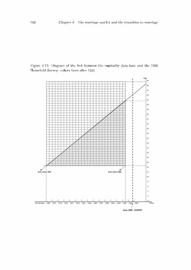
162 Chapter 4. The marriage market and the transition to marriage
Figure 4.12: Diagram of the link between the nuptiality data-base and the 1998
Household Survey: cohort born after 1955
Age50
48
46
44
42
40
38
36
34
32
30
28
26
24
22
20
18
16
14
birth cohort 1955 birth cohort 1980 12
10
8
6
4
2
0
1st January 1969 1971 1973 1975 1977 1979 1981 1983 1985 1987 1989 1991 1993 1995 1997 1999 Time
June 1998 - SURVEY
4.6. Marriage squeeze and other determinants of the transition to marriage 163
factor in the rise in delayed marriage and marital instability (Qian and Preston,
1993[147]; Goldscheider and Waite, 1986[85]). Besides the increase in the amount of
women's human capital investments, the enrollment in the educational system itself
yields a delaying e�ect in the process of family formation (Blossfeld and Huinink,
1991[25]). According to the search-theoretic framework (Oppenheimer, 1988[141])
the greater independence of women is not the cause of the reduced-gains-to-marriage
in general, but allows women to set a higher standard for the minimally acceptable
match. Therefore there is a reduction of the gains to some poor-quality marriages.
The consequence can be a delayed marriage and also a kind of increase in the risk of
non marriage as well as instability. But still, this is consistent with continued high
gains to marriage as well as with continued desire to marry.
Attending school, university, or vocational training programs is often incompat-
ible with adult family roles and activities and it can cause a postponement of the
family formation process besides increasing the economic dependence on parents.
The lack of knowledge regarding the date of end of the study period does not allow
us to reconstruct the length of the life span spent as a student for every respondent,
regardless of their �nal educational attainment. However, the level of education will
a�ect not only the period of transition into adulthood, but will have a persistent
impact also on later stages of the individual's life. Individuals with higher education
and better career opportunity increasingly delay or avoid marriage (and the same
conclusion also keeps in relation to the decision to have children). However, if mar-
riage becomes less traditional it could be sensible to expect a declining e�ect of the
educational attainment on entry into marriage (Blossfeld, 1995[69]). In a compara-
tive studies among European countries has emerged that in Italy the family system
is still traditional as the impact of educational attainment on entry into marriage is
very strong (Pinnelli and De Rose, 1995[145]).
With regard to labour market opportunities, the con icting role to the process
of union formation should be stressed again. As for education, economic theories
emphasise the gender di�erence outcome of a labour force participation. New Home
Economic theory, consider the earning power of the husband highly attractive and
disregard the wife's one as being con icting with her household production. More-
over, as we said in the �rst chapter, in traditional societies, when women do not earn

164 Chapter 4. The marriage market and the transition to marriage
any income and their value in the marriage market depends only on their ability in
household production, they have no interest in marrying late, while men who need
more time to become economically successful, postpone marriage. As a result, the
more desirable women are expected to marry the older successful men and the less
desirable women marry the young men (Oppenheimer, 1988[141]; Bergstrom and
Bagnoli, 1993[13]) .
Economic theories also focus on gender di�erential towards marriage when wage
rates increase: if the wage rates are higher for men than for women, an additional
increase of the wage rate for men will result in marrying younger, while an increase in
the wage rate for women will increase their optimal marriage age (Keeley, 1977[117]).
Sociological theories stress the importance of the attractiveness of the labour force
participation for both sexes (Oppenheimer, 1988[141]). Here it should be noted also
that we are not measuring the duration of the labour force participation, which would
require taking into account every spell of employment. Our time dependent covariate
for the job measures if one has ever worked before marrying or before the survey
time. As cohorts included at this point in the analysis are relatively recent born
cohorts (after 1955), we expect that a considerable proportion of women managed
to enter the labour market at least once in their life. Two income families are quite
spread in Italy21 and the participation to the labour force for the women before
marriage and after the end of study represents one of the most frequent models of
transition to adulthood (together with the more traditional one characterised by
the sequence: end of education and, at the same time, leaving parental home and
�rst union (Billari, 2000[18])). We expect that including the labour force experience
explanatory variable in the model of transition to �rst marriage will have a positive
impact on men and women, even though the outcome might also vary according to
age.
We do not control for premarital cohabitations, given that our aim is to study
the impact of the imbalance in the marriage market in the direct entry into �rst
marriage, and that they virtually play a competitive role to the latter on the marriage
market. In the same way, also premarital pregnancies and births are excluded from
21Employment rate for women is of about 63,7 % for woman alone and 29,7% for a women in
couple with 3 or more children (ISTAT, 2000[108])
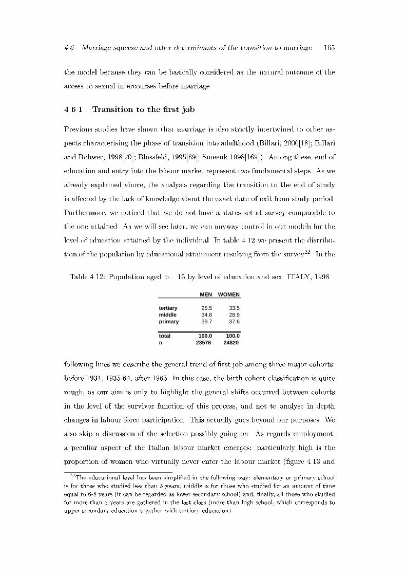
4.6. Marriage squeeze and other determinants of the transition to marriage 165
the model because they can be basically considered as the natural outcome of the
access to sexual intercourses before marriage .
4.6.1 Transition to the �rst job
Previous studies have shown that marriage is also strictly intertwined to other as-
pects characterising the phase of transition into adulthood (Billari, 2000[18]; Billari
and Rohwer, 1998[20]; Blossfeld, 1995[69]; Smeenk 1998[169]). Among these, end of
education and entry into the labour market represent two fundamental steps. As we
already explained above, the analysis regarding the transition to the end of study
is a�ected by the lack of knowledge about the exact date of exit from study period.
Furthermore, we noticed that we do not have a states set at survey comparable to
the one attained. As we will see later, we can anyway control in our models for the
level of education attained by the individual. In table 4.12 we present the distribu-
tion of the population by educational attainment resulting from the survey22. In the
Table 4.12: Population aged >= 15 by level of education and sex. ITALY, 1998
MEN WOMEN
tertiary 25.5 33.5middle 34.8 28.9primary 39.7 37.6
total 100.0 100.0n 23576 24820
following lines we describe the general trend of �rst job among three major cohorts:
before 1934, 1935-64, after 1965. In this case, the birth cohort classi�cation is quite
rough, as our aim is only to highlight the general shifts occurred between cohorts
in the level of the survivor function of this process, and not to analyse in depth
changes in labour force participation. This actually goes beyond our purposes. We
also skip a discussion of the selection possibly going on. As regards employment,
a peculiar aspect of the Italian labour market emerges: particularly high is the
proportion of women who virtually never enter the labour market (�gure 4.13 and
22The educational level has been simpli�ed in the following way: elementary or primary school
is for those who studied less than 5 years; middle is for those who studied for an amount of time
equal to 6-8 years (it can be regarded as lower secondary school) and, �nally, all those who studied
for more than 8 years are gathered in the last class (more than high school, which corresponds to
upper secondary education together with tertiary education)

166 Chapter 4. The marriage market and the transition to marriage
Table 4.13: Survivor function quartiles. First job. ITALY
quartiles <=1934 1935-44 1945-54 1955-64 >=1965 <=1934 1935-44 1945-54 1955-64 >=1965
1st quartile 14.8 15.2 15.8 16.7 17.7 18.1 17.7 17.4 18.2 19.3median 18.5 18.4 19.5 20.1 21.2 32.3 26.7 23.5 22.8 23.5
3rd quartile 23.9 22.7 23.6 23.8 25.8 42.2
WOMENMEN
Table 4.14: Survivor function at selected ages. First job. ITALY
survivors
at age <=1934 1935-44 1945-54 1955-64 >=1965 <=1934 1935-44 1945-54 1955-64 >=1965
S(15) 0.733 0.763 0.831 0.880 0.915 0.843 0.864 0.879 0.925 0.943S(20) 0.412 0.396 0.465 0.508 0.596 0.687 0.663 0.632 0.629 0.685S(25) 0.202 0.160 0.184 0.202 0.280 0.578 0.525 0.457 0.430 0.449S(30) 0.081 0.044 0.046 0.066 0.112 0.518 0.463 0.363 0.324 0.331S(35) 0.037 0.016 0.020 0.028 0.478 0.423 0.317 0.276
MEN WOMEN
tables 4.13 and 4.14). At every age, the proportion of women still outside the labour
market is high, even if decreasing across cohorts just after age 25, say after the end
of study. As a consequence, whereas only 4% of men born before 1934 never entered
the labour market, 48% of the women of the same cohort stayed outside the labour
market. Every quartile of the female distribution is reached at ages always older
than the male ones, but a relevant change in the median age at �rst employment
should be observed from the cohort born up to 1934 (reached at 32.3 years) and that
born in 1935-64 (reached at age 23.5, table 4.13). However, for every age, women
have experienced an increasing participation in the labour force from one cohort to
the following, therefore diminishing the gap, still high, with the proportion of male
labour force participation (table 4.14 and �gure 4.13). As regard the timing of the
Figure 4.13: Survivor functions by sex, cohort of birth. First job. ITALY
10 15 20 25 30 35 400
0.2
0.4
0.6
0.8
1M en
Age
Su
rviv
or
fun
ctio
ns
>=1965<=1934
1935-64
10 15 20 25 30 35 400
0.2
0.4
0.6
0.8
1W om en
Age
Su
rviv
or
fun
ctio
ns
>=1965
<=1934
1935-64
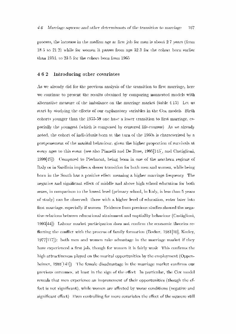
4.6. Marriage squeeze and other determinants of the transition to marriage 167
process, the increase in the median age at �rst job for men is about 2.7 years (from
18.5 to 21.2) while for women it passes from age 32.3 for the cohort born earlier
than 1934, to 23.5 for the cohort born from 1965.
4.6.2 Introducing other covariates
As we already did for the previous analysis of the transition to �rst marriage, here
we continue to present the results obtained by comparing nonnested models with
alternative measure of the imbalance on the marriage market (table 4.15). Let us
start by studying the e�ects of our explanatory variables in the Cox models. Birth
cohorts younger than the 1955-59 one have a lower transition to �rst marriage, es-
pecially the youngest (which is composed by censored life-courses). As we already
noted, the cohort of individuals born at the turn of the 1960s is characterised by a
postponement of the marital behaviour, given the higher proportion of survivals at
every ages to this event (see also Pinnelli and De Rose, 1995[145], and Castiglioni,
1999[45]). Compared to Piedmont, being born in one of the northern regions of
Italy or in Sardinia implies a slower transition for both men and women, while being
born in the South has a positive e�ect meaning a higher marriage frequency. The
negative and signi�cant e�ect of middle and above high school education for both
sexes, in comparison to the lowest level (primary school, in Italy, is less than 5 years
of study) can be observed: those with a higher level of education, enter later into
�rst marriage, especially if women. Evidence from previous studies showed the nega-
tive relations between educational attainment and nuptiality behaviour (Castiglioni,
1993[44]). Labour market participation does not con�rm the economic theories re-
ecting the con ict with the process of family formation (Becker, 1981[10], Keeley,
1977[117]): both men and women take advantage in the marriage market if they
have experienced a �rst job, though for women it is fairly weak. This con�rms the
high attractiveness played on the marital opportunities by the employment (Oppen-
heimer, 1988[141]). The female disadvantage in the marriage market con�rms our
previous outcomes, at least in the sign of the e�ect. In particular, the Cox model
reveals that men experience an improvement of their opportunities (though the ef-
fect is not signi�cant), while women are a�ected by worse conditions (negative and
signi�cant e�ect). Even controlling for more covariates the e�ect of the squeeze still
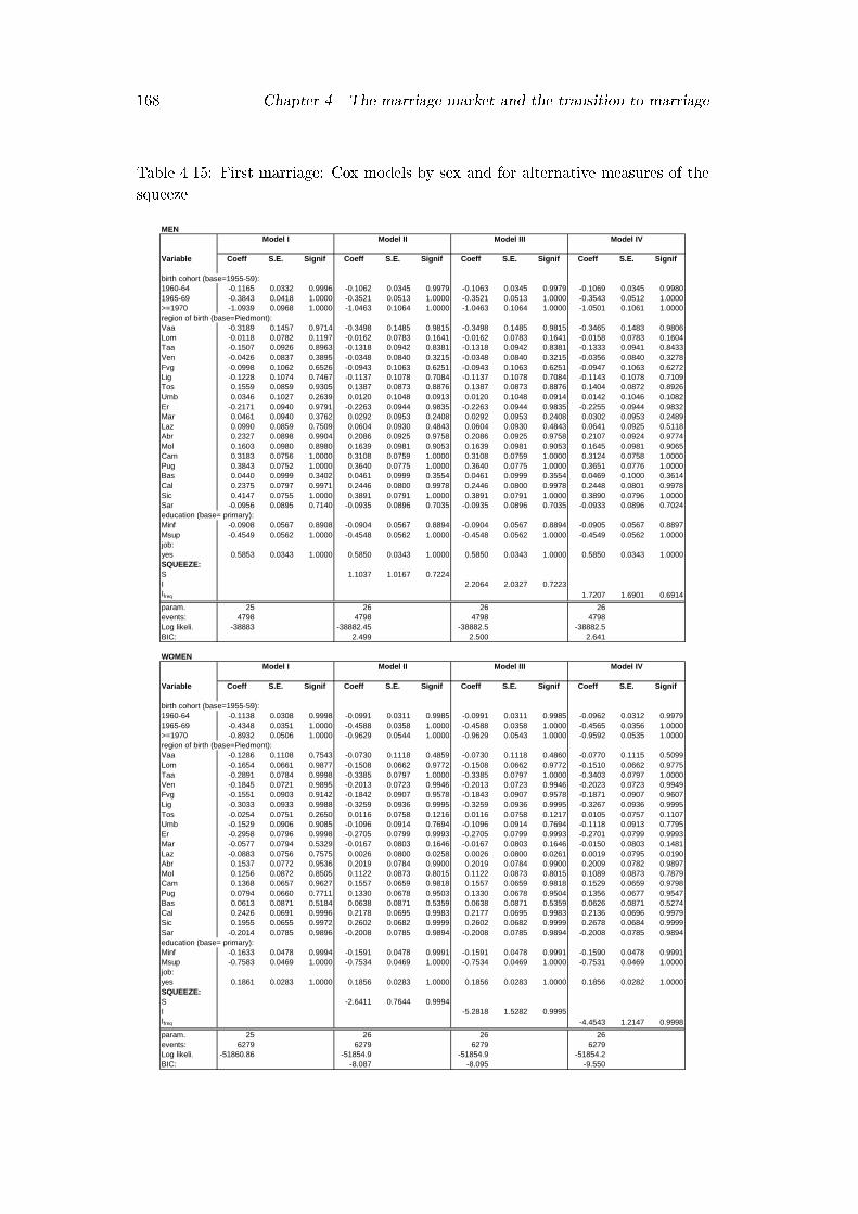
168 Chapter 4. The marriage market and the transition to marriage
Table 4.15: First marriage: Cox models by sex and for alternative measures of the
squeeze
MEN
Variable Coeff S.E. Signif Coeff S.E. Signif Coeff S.E. Signif Coeff S.E. Signif
birth cohort (base=1955-59):1960-64 -0.1165 0.0332 0.9996 -0.1062 0.0345 0.9979 -0.1063 0.0345 0.9979 -0.1069 0.0345 0.99801965-69 -0.3843 0.0418 1.0000 -0.3521 0.0513 1.0000 -0.3521 0.0513 1.0000 -0.3543 0.0512 1.0000>=1970 -1.0939 0.0968 1.0000 -1.0463 0.1064 1.0000 -1.0463 0.1064 1.0000 -1.0501 0.1061 1.0000region of birth (base=Piedmont):Vaa -0.3189 0.1457 0.9714 -0.3498 0.1485 0.9815 -0.3498 0.1485 0.9815 -0.3465 0.1483 0.9806Lom -0.0118 0.0782 0.1197 -0.0162 0.0783 0.1641 -0.0162 0.0783 0.1641 -0.0158 0.0783 0.1604Taa -0.1507 0.0926 0.8963 -0.1318 0.0942 0.8381 -0.1318 0.0942 0.8381 -0.1333 0.0941 0.8433Ven -0.0426 0.0837 0.3895 -0.0348 0.0840 0.3215 -0.0348 0.0840 0.3215 -0.0356 0.0840 0.3278Fvg -0.0998 0.1062 0.6526 -0.0943 0.1063 0.6251 -0.0943 0.1063 0.6251 -0.0947 0.1063 0.6272Lig -0.1228 0.1074 0.7467 -0.1137 0.1078 0.7084 -0.1137 0.1078 0.7084 -0.1143 0.1078 0.7109Tos 0.1559 0.0859 0.9305 0.1387 0.0873 0.8876 0.1387 0.0873 0.8876 0.1404 0.0872 0.8926Umb 0.0346 0.1027 0.2639 0.0120 0.1048 0.0913 0.0120 0.1048 0.0914 0.0142 0.1046 0.1082Er -0.2171 0.0940 0.9791 -0.2263 0.0944 0.9835 -0.2263 0.0944 0.9835 -0.2255 0.0944 0.9832Mar 0.0461 0.0940 0.3762 0.0292 0.0953 0.2408 0.0292 0.0953 0.2408 0.0302 0.0953 0.2489Laz 0.0990 0.0859 0.7509 0.0604 0.0930 0.4843 0.0604 0.0930 0.4843 0.0641 0.0925 0.5118Abr 0.2327 0.0898 0.9904 0.2086 0.0925 0.9758 0.2086 0.0925 0.9758 0.2107 0.0924 0.9774Mol 0.1603 0.0980 0.8980 0.1639 0.0981 0.9053 0.1639 0.0981 0.9053 0.1645 0.0981 0.9065Cam 0.3183 0.0756 1.0000 0.3108 0.0759 1.0000 0.3108 0.0759 1.0000 0.3124 0.0758 1.0000Pug 0.3843 0.0752 1.0000 0.3640 0.0775 1.0000 0.3640 0.0775 1.0000 0.3651 0.0776 1.0000Bas 0.0440 0.0999 0.3402 0.0461 0.0999 0.3554 0.0461 0.0999 0.3554 0.0469 0.1000 0.3614Cal 0.2375 0.0797 0.9971 0.2446 0.0800 0.9978 0.2446 0.0800 0.9978 0.2448 0.0801 0.9978Sic 0.4147 0.0755 1.0000 0.3891 0.0791 1.0000 0.3891 0.0791 1.0000 0.3890 0.0796 1.0000Sar -0.0956 0.0895 0.7140 -0.0935 0.0896 0.7035 -0.0935 0.0896 0.7035 -0.0933 0.0896 0.7024education (base= primary):Minf -0.0908 0.0567 0.8908 -0.0904 0.0567 0.8894 -0.0904 0.0567 0.8894 -0.0905 0.0567 0.8897Msup -0.4549 0.0562 1.0000 -0.4548 0.0562 1.0000 -0.4548 0.0562 1.0000 -0.4549 0.0562 1.0000job:yes 0.5853 0.0343 1.0000 0.5850 0.0343 1.0000 0.5850 0.0343 1.0000 0.5850 0.0343 1.0000SQUEEZE:S 1.1037 1.0167 0.7224I 2.2064 2.0327 0.7223Ifreq 1.7207 1.6901 0.6914
param. 25 26 26 26events: 4798 4798 4798 4798Log likeli. -38883 -38882.45 -38882.5 -38882.5BIC: 2.499 2.500 2.641
WOMEN
Variable Coeff S.E. Signif Coeff S.E. Signif Coeff S.E. Signif Coeff S.E. Signif
birth cohort (base=1955-59):1960-64 -0.1138 0.0308 0.9998 -0.0991 0.0311 0.9985 -0.0991 0.0311 0.9985 -0.0962 0.0312 0.99791965-69 -0.4348 0.0351 1.0000 -0.4588 0.0358 1.0000 -0.4588 0.0358 1.0000 -0.4565 0.0356 1.0000>=1970 -0.8932 0.0506 1.0000 -0.9629 0.0544 1.0000 -0.9629 0.0543 1.0000 -0.9592 0.0535 1.0000region of birth (base=Piedmont):Vaa -0.1286 0.1108 0.7543 -0.0730 0.1118 0.4859 -0.0730 0.1118 0.4860 -0.0770 0.1115 0.5099Lom -0.1654 0.0661 0.9877 -0.1508 0.0662 0.9772 -0.1508 0.0662 0.9772 -0.1510 0.0662 0.9775Taa -0.2891 0.0784 0.9998 -0.3385 0.0797 1.0000 -0.3385 0.0797 1.0000 -0.3403 0.0797 1.0000Ven -0.1845 0.0721 0.9895 -0.2013 0.0723 0.9946 -0.2013 0.0723 0.9946 -0.2023 0.0723 0.9949Fvg -0.1551 0.0903 0.9142 -0.1842 0.0907 0.9578 -0.1843 0.0907 0.9578 -0.1871 0.0907 0.9607Lig -0.3033 0.0933 0.9988 -0.3259 0.0936 0.9995 -0.3259 0.0936 0.9995 -0.3267 0.0936 0.9995Tos -0.0254 0.0751 0.2650 0.0116 0.0758 0.1216 0.0116 0.0758 0.1217 0.0105 0.0757 0.1107Umb -0.1529 0.0906 0.9085 -0.1096 0.0914 0.7694 -0.1096 0.0914 0.7694 -0.1118 0.0913 0.7795Er -0.2958 0.0796 0.9998 -0.2705 0.0799 0.9993 -0.2705 0.0799 0.9993 -0.2701 0.0799 0.9993Mar -0.0577 0.0794 0.5329 -0.0167 0.0803 0.1646 -0.0167 0.0803 0.1646 -0.0150 0.0803 0.1481Laz -0.0883 0.0756 0.7575 0.0026 0.0800 0.0258 0.0026 0.0800 0.0261 0.0019 0.0795 0.0190Abr 0.1537 0.0772 0.9536 0.2019 0.0784 0.9900 0.2019 0.0784 0.9900 0.2009 0.0782 0.9897Mol 0.1256 0.0872 0.8505 0.1122 0.0873 0.8015 0.1122 0.0873 0.8015 0.1089 0.0873 0.7879Cam 0.1368 0.0657 0.9627 0.1557 0.0659 0.9818 0.1557 0.0659 0.9818 0.1529 0.0659 0.9798Pug 0.0794 0.0660 0.7711 0.1330 0.0678 0.9503 0.1330 0.0678 0.9504 0.1356 0.0677 0.9547Bas 0.0613 0.0871 0.5184 0.0638 0.0871 0.5359 0.0638 0.0871 0.5359 0.0626 0.0871 0.5274Cal 0.2426 0.0691 0.9996 0.2178 0.0695 0.9983 0.2177 0.0695 0.9983 0.2136 0.0696 0.9979Sic 0.1955 0.0655 0.9972 0.2602 0.0682 0.9999 0.2602 0.0682 0.9999 0.2678 0.0684 0.9999Sar -0.2014 0.0785 0.9896 -0.2008 0.0785 0.9894 -0.2008 0.0785 0.9894 -0.2008 0.0785 0.9894education (base= primary):Minf -0.1633 0.0478 0.9994 -0.1591 0.0478 0.9991 -0.1591 0.0478 0.9991 -0.1590 0.0478 0.9991Msup -0.7583 0.0469 1.0000 -0.7534 0.0469 1.0000 -0.7534 0.0469 1.0000 -0.7531 0.0469 1.0000job:yes 0.1861 0.0283 1.0000 0.1856 0.0283 1.0000 0.1856 0.0283 1.0000 0.1856 0.0282 1.0000SQUEEZE:S -2.6411 0.7644 0.9994I -5.2818 1.5282 0.9995Ifreq -4.4543 1.2147 0.9998
param. 25 26 26 26events: 6279 6279 6279 6279Log likeli. -51860.86 -51854.9 -51854.9 -51854.2BIC: -8.087 -8.095 -9.550
Model I Model II Model III Model IV
Model I Model II Model III Model IV

4.6. Marriage squeeze and other determinants of the transition to marriage 169
holds. The comparison between Model II, III and IV shows that the best, according
to the BIC criterion is, for men the one using S as a squeeze measure and for women
the one based on Ifreq (table 4.15).
The outcomes provided by the piecewise constant exponential model go in the
same direction emerged and show the same e�ects and sign of the explanatory vari-
ables obtained from the Cox model. Younger cohorts have a much lower rate of
transition than old ones. People born in the South marry earlier than those born in
the North. Studying longer, therefore attaining a higher level of education, means
a delaying e�ect on �rst marriage (due to a negative and signi�cant e�ect) for men
and women: there is an increasing delay in marrying for younger birth cohorts in
comparison to the 1955-59 one. In particular, men with middle education have prac-
tically the same conditions of those with elementary level of education. Given that
our set of individuals is composed by relatively young people (born after 1955) for
which there has been an increasing involvement in longer period of study, but men
always had a higher participation in the educational system, the two groups (with
elementary and middle education) might include very selected men. Their position
is quite bad with respect to the education attained and, as a consequence their
position in the marriage market is also very disadvantaged. Experiencing a job for
men means increasing marriage opportunities and a decreasing (negative but weaker
coe�cients) for female transition to �rst marriage (in both cases it has a signi�cant
e�ect). The age pattern described by the piecewise constant function is bell-shaped.
Men and women di�er in the e�ect of the squeeze, as it can make the former marry
earlier and the latter later. From the BIC statistic the best model, for women, is
the one obtained by using the measure Ifreq, and for men as well (tables 4.16 and
4.17, Model III). Lastly, a piecewise constant exponential model with period speci�c
e�ects for the same set of covariates has been modeled (tables 4.18 and 4.19).
It was not possible to estimate the age e�ect for the birth cohorts under study
because they include too young individuals. As shown in �gure 4.12, at the end of
1995, those born in 1970 are no more than 25 years old and, as a consequence, it is
not possible to estimate the coe�cient above that age. For comparative purposes and
to avoid right censoring problems, the youngest cohorts should be disregarded. If we
eliminate those born after 1970, then we can estimate the coe�cient, divided into
170 Chapter 4. The marriage market and the transition to marriage
Table 4.16: First marriage: e�ect of the imbalance in the marriage market estimated
by the piecewise constant exponential models: MEN
MEN
Variable Coeff S.E. Signif Coeff S.E. Signif Coeff S.E. Signif
[15,23) -6.8239 0.0875 1.0000 -6.8239 0.0875 1.0000 -6.8253 0.0875 1.0000[23,25) -5.2360 0.0889 1.0000 -5.2360 0.0889 1.0000 -5.2409 0.0889 1.0000[25,27) -4.8745 0.0885 1.0000 -4.8745 0.0885 1.0000 -4.8788 0.0886 1.0000[27,29) -4.6463 0.0893 1.0000 -4.6463 0.0893 1.0000 -4.6492 0.0893 1.0000[29,32) -4.6916 0.0908 1.0000 -4.6916 0.0908 1.0000 -4.6926 0.0908 1.0000[32,+) -5.0464 0.0985 1.0000 -5.0464 0.0985 1.0000 -5.0451 0.0982 1.0000birth cohort (base=1955-59):1960-64 -0.0686 0.0343 0.9542 -0.0686 0.0343 0.9542 -0.0669 0.0343 0.94911965-69 -0.2689 0.0486 1.0000 -0.2689 0.0486 1.0000 -0.2646 0.0482 1.0000>=1970 -1.1661 0.1028 1.0000 -1.1661 0.1028 1.0000 -1.1618 0.1024 1.0000region of birth (base=Piedmont):Vaa -0.4283 0.1483 0.9961 -0.4284 0.1483 0.9961 -0.4298 0.1480 0.9963Lom -0.0212 0.0783 0.2130 -0.0212 0.0783 0.2130 -0.0217 0.0783 0.2185Taa -0.0874 0.0940 0.6472 -0.0874 0.0940 0.6471 -0.0842 0.0940 0.6299Ven -0.0203 0.0840 0.1914 -0.0203 0.0840 0.1913 -0.0189 0.0840 0.1779Fvg -0.0794 0.1063 0.5451 -0.0794 0.1063 0.5451 -0.0778 0.1063 0.5359Lig -0.0950 0.1077 0.6222 -0.0950 0.1077 0.6222 -0.0930 0.1077 0.6122Tos 0.1106 0.0871 0.7958 0.1106 0.0871 0.7958 0.1095 0.0870 0.7919Umb -0.0309 0.1044 0.2323 -0.0309 0.1044 0.2323 -0.0325 0.1043 0.2450Er -0.2518 0.0943 0.9924 -0.2518 0.0943 0.9924 -0.2531 0.0943 0.9927Mar -0.0015 0.0951 0.0124 -0.0015 0.0951 0.0125 -0.0053 0.0950 0.0447Laz -0.0094 0.0920 0.0814 -0.0094 0.0920 0.0816 -0.0135 0.0914 0.1172Abr 0.1734 0.0921 0.9403 0.1734 0.0921 0.9403 0.1709 0.0919 0.9370Mol 0.1860 0.0980 0.9421 0.1860 0.0980 0.9421 0.1902 0.0981 0.9475Cam 0.3170 0.0758 1.0000 0.3170 0.0758 1.0000 0.3195 0.0757 1.0000Pug 0.3369 0.0773 1.0000 0.3369 0.0773 1.0000 0.3314 0.0773 1.0000Bas 0.0651 0.0999 0.4851 0.0651 0.0999 0.4851 0.0686 0.0999 0.5072Cal 0.2736 0.0800 0.9994 0.2736 0.0800 0.9994 0.2783 0.0800 0.9995Sic 0.3449 0.0786 1.0000 0.3449 0.0786 1.0000 0.3326 0.0790 1.0000Sar -0.0789 0.0896 0.6217 -0.0789 0.0896 0.6217 -0.0778 0.0896 0.6149education (base <=elementary):middle -0.0956 0.0567 0.9083 -0.0956 0.0567 0.9083 -0.0956 0.0567 0.9085>=high school -0.4495 0.0562 1.0000 -0.4495 0.0562 1.0000 -0.4495 0.0562 1.0000Squeeze S by region of birth Squeeze I by region of birth Squeeze I freq by region of birth
SmuB 3.4864 0.9417 0.9998 6.9716 1.8829 0.9998 6.1800 1.5404 0.9999Jobyes 0.7564 0.0355 1.0000 0.7564 0.0355 1.0000 0.7558 0.0355 1.0000
n. parameters 32 32 32n. constraintsn. events 4798 4798 4798n. episodes 116515 116515 116515Log-likelihood: -28288.94 -28288.94 -28287.7BIC: -21162.43 -21162.44 -21164.92
Model IIIModel I Model II

4.6. Marriage squeeze and other determinants of the transition to marriage 171
Table 4.17: First marriage: e�ect of the imbalance in the marriage market estimated
by the piecewise constant exponential models: WOMEN
WOMEN
Variable Coeff S.E. Signif Coeff S.E. Signif Coeff S.E. Signif
[15,18) -6.5732 0.0918 1.0000 -6.5732 0.0918 1.0000 -6.5778 0.0919 1.0000[18,20) -4.5732 0.0730 1.0000 -4.5732 0.0730 1.0000 -4.5756 0.0730 1.0000[20,22) -4.1095 0.0727 1.0000 -4.1095 0.0727 1.0000 -4.1100 0.0727 1.0000[22,24) -3.8532 0.0738 1.0000 -3.8532 0.0738 1.0000 -3.8532 0.0738 1.0000[24,26) -3.6626 0.0757 1.0000 -3.6627 0.0757 1.0000 -3.6628 0.0757 1.0000[26,28) -3.7063 0.0801 1.0000 -3.7063 0.0801 1.0000 -3.7069 0.0801 1.0000[28,30) -3.8089 0.0871 1.0000 -3.8089 0.0871 1.0000 -3.8100 0.0871 1.0000[30,+) -4.3098 0.0893 1.0000 -4.3098 0.0893 1.0000 -4.3115 0.0891 1.0000birth cohort (base=1955-59):1960-64 -0.0790 0.0311 0.9889 -0.0790 0.0311 0.9889 -0.0765 0.0312 0.98571965-69 -0.4309 0.0358 1.0000 -0.4309 0.0358 1.0000 -0.4302 0.0356 1.0000>=1970 -0.9227 0.0543 1.0000 -0.9228 0.0543 1.0000 -0.9226 0.0535 1.0000region of birth (base=Piedmont):Vaa -0.0931 0.1119 0.5948 -0.0931 0.1119 0.5948 -0.0940 0.1116 0.6003Lom -0.1580 0.0662 0.9830 -0.1579 0.0662 0.9830 -0.1576 0.0662 0.9827Taa -0.3239 0.0797 1.0000 -0.3240 0.0797 1.0000 -0.3269 0.0796 1.0000Ven -0.1998 0.0723 0.9943 -0.1998 0.0723 0.9943 -0.2011 0.0723 0.9946Fvg -0.1755 0.0907 0.9471 -0.1755 0.0907 0.9472 -0.1785 0.0907 0.9510Lig -0.3169 0.0936 0.9993 -0.3169 0.0936 0.9993 -0.3183 0.0936 0.9993Tos -0.0005 0.0758 0.0056 -0.0005 0.0758 0.0055 0.0000 0.0757 0.0001Umb -0.1241 0.0915 0.8252 -0.1241 0.0915 0.8252 -0.1241 0.0913 0.8261Er -0.2837 0.0799 0.9996 -0.2837 0.0799 0.9996 -0.2825 0.0799 0.9996Mar -0.0307 0.0803 0.2974 -0.0306 0.0803 0.2973 -0.0280 0.0802 0.2728Laz -0.0334 0.0800 0.3235 -0.0333 0.0800 0.3231 -0.0307 0.0794 0.3004Abr 0.1874 0.0784 0.9831 0.1874 0.0784 0.9831 0.1883 0.0782 0.9839Mol 0.1133 0.0872 0.8061 0.1133 0.0872 0.8061 0.1105 0.0873 0.7946Cam 0.1466 0.0659 0.9738 0.1466 0.0659 0.9738 0.1453 0.0659 0.9727Pug 0.1127 0.0677 0.9038 0.1127 0.0677 0.9038 0.1164 0.0677 0.9145Bas 0.0523 0.0871 0.4518 0.0523 0.0871 0.4518 0.0515 0.0871 0.4456Cal 0.2218 0.0695 0.9986 0.2218 0.0695 0.9986 0.2179 0.0696 0.9983Sic 0.2377 0.0681 0.9995 0.2377 0.0681 0.9995 0.2454 0.0684 0.9997Sar -0.2011 0.0785 0.9896 -0.2011 0.0785 0.9896 -0.2011 0.0785 0.9895education (base <=elementary):middle -0.1637 0.0478 0.9994 -0.1637 0.0478 0.9994 -0.1635 0.0478 0.9994>=high school -0.7579 0.0469 1.0000 -0.7579 0.0469 1.0000 -0.7575 0.0469 1.0000Squeeze S by region of birth Squeeze I by region of birth Squeeze I freq by region of birth
SmuB -1.8123 0.7627 0.9825 -3.6251 1.5247 0.9826 -3.2149 1.2133 0.9919Jobyes 0.1836 0.0283 1.0000 0.1836 0.0283 1.0000 0.1836 0.0283 1.0000
n. parameters 34 34 34n. constraintsn. events 6279 6279 6279n. episodes 98533 98533 98533Log-likelihood: -35769.8 -35769.8 -35769.13BIC: -32147.93 -32147.94 -32149.29
Model I Model II Model III

172 Chapter 4. The marriage market and the transition to marriage
age subgroups, for all other cohorts up to age 25. Even so, the gains of estimating the
other covariates would not improve much, and this leads us to consider the general
e�ect associated to a given birth cohort. The e�ect of this birth cohort follows what
we said above for the previous models.
Men with middle educational level, especially if younger than 23 years, have a
transition to �rst marriage lower than those with the elementary level up to age 27,
after that age the transition rate has an incresing e�ect (positive coe�cient) and in
comparison to those with lower education they show a catching up e�ect. The same
behaviour, as it emerged for middle educated men, is shared by those in the highest
category of education (more than high education). There is no forgoing in marriage,
but a postponement e�ect.
As regards the e�ect of the imbalance in the marriage market , men have always
a positive and U-shaped e�ect, regardless of the age groups 23-25 and 27-29 when
it is negative but not signi�cant. The experience of a �rst job for men is always
signi�cant and induces them to marry earlier than those without job. The very high
coe�cient 1.2289 for the men in age group 15-23, needs some comments. This group
is compared to young men who never worked up to age 23. Therefore, the group
which they are compared to is mainly composed by students or, selected men (for
instance, if they are not students, they might be ill or in the military service). They
represent a very selected group of individuals, and in their respect men who enter in
a �rst job also have greater marriage opportunities. All other age groups of men take
advantage of the positive and signi�cant e�ect of the �rst job experience, therefore
they marry earlier. In all these cases the e�ect is not very strong, probably because
in these age groups, only few men have never worked at all: we are comparing the
e�ect of transition to �rst marriage of men who entered the labour market at least
once, to a selected and small group of individuals out of the labour market (for
instance, ill people). The transition rates for both sexes are reported in �gure 4.14:
the age-pattern associated to �rst marriage and described by the piecewise constant,
is bell shaped.
As regard women, the e�ect of the birth cohort, as well as that of region of
birth is the same as for men. The age e�ects of the attained level of education are
quite interesting. For each level of education attained by the women, there is a

4.6. Marriage squeeze and other determinants of the transition to marriage 173
Table 4.18: First marriage: age e�ect of the imbalance in the marriage market
estimated by the piecewise constant exponential models: MEN
MEN
Variable Coeff S.E. Signif Coeff S.E. Signif Coeff S.E. Signif
[15,23) -6.4741 0.1156 1.0000 -6.4740 0.1156 1.0000 -6.4715 0.1156 1.0000[23,25) -4.8476 0.1317 1.0000 -4.8476 0.1317 1.0000 -4.8485 0.1319 1.0000[25,27) -4.6796 0.1380 1.0000 -4.6796 0.1380 1.0000 -4.6832 0.1382 1.0000[27,29) -4.9667 0.1804 1.0000 -4.9666 0.1804 1.0000 -4.9677 0.1805 1.0000[29,32) -4.9080 0.1913 1.0000 -4.9080 0.1913 1.0000 -4.9106 0.1914 1.0000[32,+) -6.2036 0.3270 1.0000 -6.2036 0.3270 1.0000 -6.2035 0.3270 1.0000birth cohort (base=1955-59):1960-64 -0.0886 0.0362 0.9856 -0.0886 0.0362 0.9856 -0.0885 0.0364 0.98511965-69 -0.3288 0.0528 1.0000 -0.3288 0.0528 1.0000 -0.3278 0.0529 1.0000>=1970 -1.0909 0.1049 1.0000 -1.0909 0.1049 1.0000 -1.0942 0.1044 1.0000region of birth (base=Piedmont):Vaa -0.4109 0.1486 0.9943 -0.4109 0.1486 0.9943 -0.4084 0.1484 0.9941Lom -0.0272 0.0783 0.2715 -0.0272 0.0783 0.2714 -0.0267 0.0783 0.2671Taa -0.0982 0.0942 0.7029 -0.0982 0.0942 0.7029 -0.0970 0.0941 0.6972Ven -0.0236 0.0840 0.2210 -0.0236 0.0840 0.2210 -0.0223 0.0840 0.2091Fvg -0.0687 0.1063 0.4814 -0.0686 0.1063 0.4814 -0.0682 0.1063 0.4784Lig -0.0965 0.1078 0.6295 -0.0965 0.1078 0.6295 -0.0957 0.1078 0.6252Tos 0.1127 0.0873 0.8035 0.1127 0.0873 0.8035 0.1136 0.0872 0.8075Umb -0.0090 0.1048 0.0682 -0.0090 0.1048 0.0681 -0.0081 0.1048 0.0619Er -0.2283 0.0944 0.9844 -0.2283 0.0944 0.9844 -0.2285 0.0944 0.9846Mar -0.0030 0.0951 0.0250 -0.0030 0.0951 0.0250 -0.0046 0.0951 0.0386Laz 0.0005 0.0923 0.0047 0.0005 0.0923 0.0046 0.0007 0.0920 0.0060Abr 0.1921 0.0924 0.9624 0.1921 0.0924 0.9624 0.1926 0.0923 0.9630Mol 0.1631 0.0982 0.9034 0.1631 0.0982 0.9034 0.1663 0.0982 0.9096Cam 0.2942 0.0759 0.9999 0.2942 0.0759 0.9999 0.2979 0.0758 0.9999Pug 0.3101 0.0774 0.9999 0.3101 0.0774 0.9999 0.3079 0.0775 0.9999Bas 0.0418 0.1000 0.3241 0.0418 0.1000 0.3240 0.0444 0.1000 0.3426Cal 0.2650 0.0802 0.9990 0.2650 0.0802 0.9990 0.2687 0.0802 0.9992Sic 0.3284 0.0789 1.0000 0.3284 0.0789 1.0000 0.3203 0.0794 0.9999Sar -0.0743 0.0896 0.5928 -0.0743 0.0896 0.5928 -0.0739 0.0896 0.5904education (base <=elementary):Middle[15,23) -0.6098 0.1013 1.0000 -0.6098 0.1013 1.0000 -0.6106 0.1013 1.0000[23,25) -0.1455 0.1158 0.7910 -0.1455 0.1158 0.7910 -0.1455 0.1158 0.7910[25,27) -0.2062 0.1221 0.9087 -0.2062 0.1221 0.9087 -0.2058 0.1221 0.9080[27,29) 0.3490 0.1695 0.9605 0.3490 0.1695 0.9605 0.3497 0.1695 0.9609[29,32) 0.3811 0.1870 0.9585 0.3811 0.1870 0.9585 0.3816 0.1870 0.9587[32,+) 1.0349 0.3200 0.9988 1.0349 0.3200 0.9988 1.0334 0.3200 0.9988>=high school[15,23) -1.3523 0.1135 1.0000 -1.3523 0.1135 1.0000 -1.3529 0.1135 1.0000[23,25) -0.8300 0.1189 1.0000 -0.8300 0.1189 1.0000 -0.8300 0.1189 1.0000[25,27) -0.4954 0.1203 1.0000 -0.4954 0.1203 1.0000 -0.4951 0.1203 1.0000[27,29) 0.1189 0.1670 0.5235 0.1189 0.1670 0.5235 0.1194 0.1670 0.5253[29,32) 0.3227 0.1826 0.9228 0.3227 0.1826 0.9228 0.3231 0.1826 0.9231[32,+) 1.3055 0.3133 1.0000 1.3055 0.3133 1.0000 1.3047 0.3133 1.0000Squeeze S by region of birth Squeeze I by region of birth Squeeze I freq by region of birth[15,23) 7.3306 1.7718 1.0000 14.6583 3.5420 1.0000 11.8231 2.6925 1.0000[23,25) -0.4510 1.7403 0.2045 -0.9020 3.4795 0.2045 -0.5550 2.8624 0.1537[25,27) 3.3720 1.6017 0.9647 6.7415 3.2025 0.9647 5.6693 2.6747 0.9660[27,29) -0.1808 1.6130 0.0892 -0.3615 3.2250 0.0892 -0.1515 2.7321 0.0442[29,32) 4.6714 1.7728 0.9916 9.3399 3.5446 0.9916 8.1337 3.0316 0.9927[32,+) 7.6609 2.6855 0.9957 15.3179 5.3696 0.9957 13.2364 4.6788 0.9953Job[15,23) 1.2289 0.0739 1.0000 1.2289 0.0739 1.0000 1.2263 0.0739 1.0000[23,25) 0.5512 0.0719 1.0000 0.5512 0.0719 1.0000 0.5512 0.0719 1.0000[25,27) 0.6321 0.0728 1.0000 0.6321 0.0728 1.0000 0.6322 0.0728 1.0000[27,29) 0.5915 0.0838 1.0000 0.5915 0.0838 1.0000 0.5915 0.0838 1.0000[29,32) 0.2941 0.0939 0.9983 0.2941 0.0939 0.9983 0.2938 0.0939 0.9982[32,+) 0.5240 0.1749 0.9973 0.5240 0.1749 0.9973 0.5223 0.1749 0.9972
n. parameters 162 162 162n. constraints 110 110 110n. events 4798 4798 4798n. episodes 116515 116515 116515Log-likelihood: -28134.98 -28134.97 -28133.86BIC: -21396.74 -21396.75 -21398.98
Model I Model II Model III

174 Chapter 4. The marriage market and the transition to marriage
postponement e�ect (negative and signi�cant coe�cient) up to around age 26; after
that age, coe�cients, even if weak, are positive. Women with the middle level of
education have a transition rate lower then the one for those with the elementary
level, up to age 26; then, the coe�cient of the rate becomes positive: actually, the
di�erences with low educated women are not striking and also the e�ects are not
very signi�cant. On the contrary, for those with high level of education there is a
clear, signi�cant and negative e�ect up to age 26 (but those in the age group 15-18
are still involved in studying, at least for the lowest level of this category). After
that age, the attained educational level has a high impact on the experience of �rst
marriage if compared to the one with elementary level. Women age more than 30
years and high level of education could also represents a selected group, given the
relatively small number of members with high education.
Despite the lack of information about the end of study, which prevents us from
including the amount of years spent in the educational system and their ending
time, the model shows the postponement e�ect associated with every level of edu-
cation. It is not clear whether the postponement will eventually also cause a lower
proportion of total marriages for those with, for instance, high education. Increas-
ing human capital discourages early marriages, but is not incompatible to marriage
(Oppenheimer, 1988[141]).
The e�ect of the squeeze by region of birth for women, even though not signi�-
Figure 4.14: Transition rate for the piecewise constant exponential model by sex:
Piedmont, birth cohort 1955-1964
15 20 25 30 35 40 45 500
0.01
0.02
0.03
M E N
W O M E N
Age
Tra
nsiti
on r
ate
(bas
elin
e)
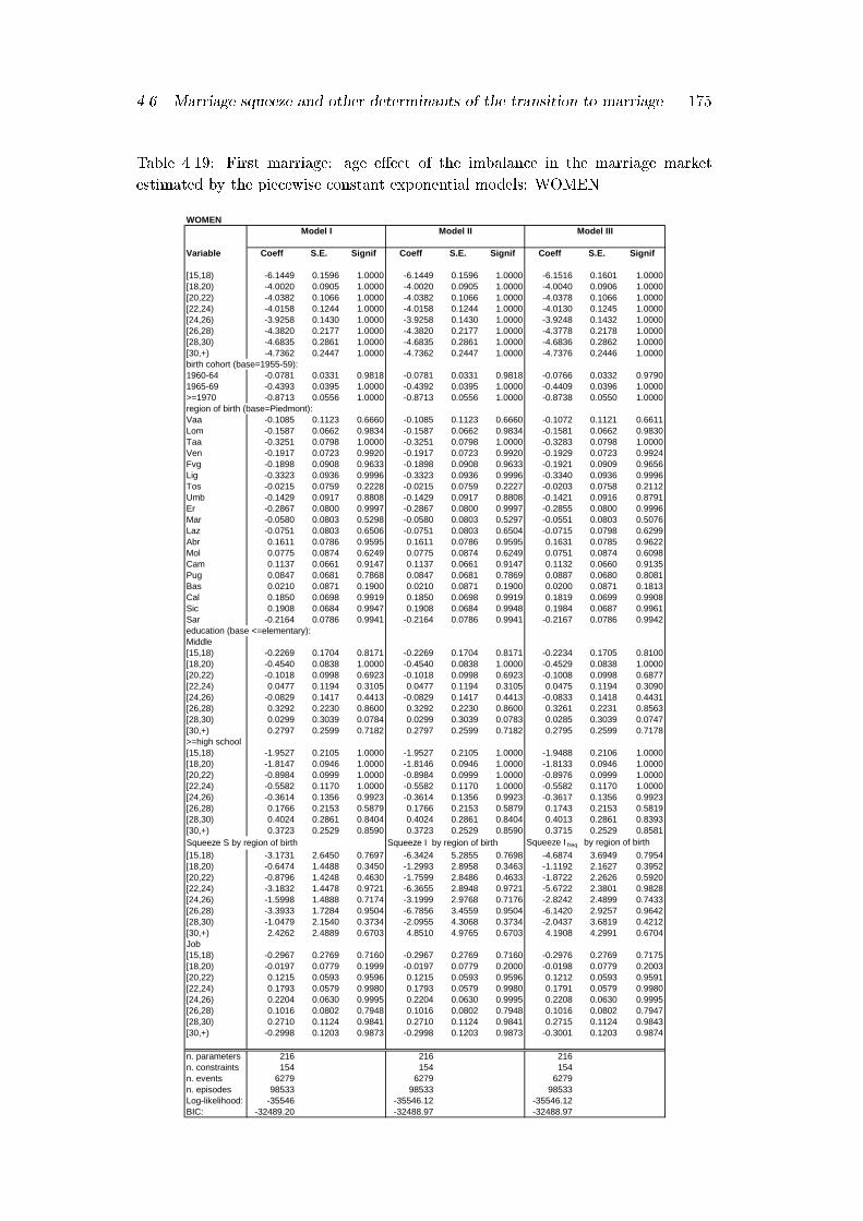
4.6. Marriage squeeze and other determinants of the transition to marriage 175
Table 4.19: First marriage: age e�ect of the imbalance in the marriage market
estimated by the piecewise constant exponential models: WOMEN
WOMEN
Variable Coeff S.E. Signif Coeff S.E. Signif Coeff S.E. Signif
[15,18) -6.1449 0.1596 1.0000 -6.1449 0.1596 1.0000 -6.1516 0.1601 1.0000[18,20) -4.0020 0.0905 1.0000 -4.0020 0.0905 1.0000 -4.0040 0.0906 1.0000[20,22) -4.0382 0.1066 1.0000 -4.0382 0.1066 1.0000 -4.0378 0.1066 1.0000[22,24) -4.0158 0.1244 1.0000 -4.0158 0.1244 1.0000 -4.0130 0.1245 1.0000[24,26) -3.9258 0.1430 1.0000 -3.9258 0.1430 1.0000 -3.9248 0.1432 1.0000[26,28) -4.3820 0.2177 1.0000 -4.3820 0.2177 1.0000 -4.3778 0.2178 1.0000[28,30) -4.6835 0.2861 1.0000 -4.6835 0.2861 1.0000 -4.6836 0.2862 1.0000[30,+) -4.7362 0.2447 1.0000 -4.7362 0.2447 1.0000 -4.7376 0.2446 1.0000birth cohort (base=1955-59):1960-64 -0.0781 0.0331 0.9818 -0.0781 0.0331 0.9818 -0.0766 0.0332 0.97901965-69 -0.4393 0.0395 1.0000 -0.4392 0.0395 1.0000 -0.4409 0.0396 1.0000>=1970 -0.8713 0.0556 1.0000 -0.8713 0.0556 1.0000 -0.8738 0.0550 1.0000region of birth (base=Piedmont):Vaa -0.1085 0.1123 0.6660 -0.1085 0.1123 0.6660 -0.1072 0.1121 0.6611Lom -0.1587 0.0662 0.9834 -0.1587 0.0662 0.9834 -0.1581 0.0662 0.9830Taa -0.3251 0.0798 1.0000 -0.3251 0.0798 1.0000 -0.3283 0.0798 1.0000Ven -0.1917 0.0723 0.9920 -0.1917 0.0723 0.9920 -0.1929 0.0723 0.9924Fvg -0.1898 0.0908 0.9633 -0.1898 0.0908 0.9633 -0.1921 0.0909 0.9656Lig -0.3323 0.0936 0.9996 -0.3323 0.0936 0.9996 -0.3340 0.0936 0.9996Tos -0.0215 0.0759 0.2228 -0.0215 0.0759 0.2227 -0.0203 0.0758 0.2112Umb -0.1429 0.0917 0.8808 -0.1429 0.0917 0.8808 -0.1421 0.0916 0.8791Er -0.2867 0.0800 0.9997 -0.2867 0.0800 0.9997 -0.2855 0.0800 0.9996Mar -0.0580 0.0803 0.5298 -0.0580 0.0803 0.5297 -0.0551 0.0803 0.5076Laz -0.0751 0.0803 0.6506 -0.0751 0.0803 0.6504 -0.0715 0.0798 0.6299Abr 0.1611 0.0786 0.9595 0.1611 0.0786 0.9595 0.1631 0.0785 0.9622Mol 0.0775 0.0874 0.6249 0.0775 0.0874 0.6249 0.0751 0.0874 0.6098Cam 0.1137 0.0661 0.9147 0.1137 0.0661 0.9147 0.1132 0.0660 0.9135Pug 0.0847 0.0681 0.7868 0.0847 0.0681 0.7869 0.0887 0.0680 0.8081Bas 0.0210 0.0871 0.1900 0.0210 0.0871 0.1900 0.0200 0.0871 0.1813Cal 0.1850 0.0698 0.9919 0.1850 0.0698 0.9919 0.1819 0.0699 0.9908Sic 0.1908 0.0684 0.9947 0.1908 0.0684 0.9948 0.1984 0.0687 0.9961Sar -0.2164 0.0786 0.9941 -0.2164 0.0786 0.9941 -0.2167 0.0786 0.9942education (base <=elementary):Middle[15,18) -0.2269 0.1704 0.8171 -0.2269 0.1704 0.8171 -0.2234 0.1705 0.8100[18,20) -0.4540 0.0838 1.0000 -0.4540 0.0838 1.0000 -0.4529 0.0838 1.0000[20,22) -0.1018 0.0998 0.6923 -0.1018 0.0998 0.6923 -0.1008 0.0998 0.6877[22,24) 0.0477 0.1194 0.3105 0.0477 0.1194 0.3105 0.0475 0.1194 0.3090[24,26) -0.0829 0.1417 0.4413 -0.0829 0.1417 0.4413 -0.0833 0.1418 0.4431[26,28) 0.3292 0.2230 0.8600 0.3292 0.2230 0.8600 0.3261 0.2231 0.8563[28,30) 0.0299 0.3039 0.0784 0.0299 0.3039 0.0783 0.0285 0.3039 0.0747[30,+) 0.2797 0.2599 0.7182 0.2797 0.2599 0.7182 0.2795 0.2599 0.7178>=high school[15,18) -1.9527 0.2105 1.0000 -1.9527 0.2105 1.0000 -1.9488 0.2106 1.0000[18,20) -1.8147 0.0946 1.0000 -1.8146 0.0946 1.0000 -1.8133 0.0946 1.0000[20,22) -0.8984 0.0999 1.0000 -0.8984 0.0999 1.0000 -0.8976 0.0999 1.0000[22,24) -0.5582 0.1170 1.0000 -0.5582 0.1170 1.0000 -0.5582 0.1170 1.0000[24,26) -0.3614 0.1356 0.9923 -0.3614 0.1356 0.9923 -0.3617 0.1356 0.9923[26,28) 0.1766 0.2153 0.5879 0.1766 0.2153 0.5879 0.1743 0.2153 0.5819[28,30) 0.4024 0.2861 0.8404 0.4024 0.2861 0.8404 0.4013 0.2861 0.8393[30,+) 0.3723 0.2529 0.8590 0.3723 0.2529 0.8590 0.3715 0.2529 0.8581Squeeze S by region of birth Squeeze I by region of birth Squeeze I freq by region of birth
[15,18) -3.1731 2.6450 0.7697 -6.3424 5.2855 0.7698 -4.6874 3.6949 0.7954[18,20) -0.6474 1.4488 0.3450 -1.2993 2.8958 0.3463 -1.1192 2.1627 0.3952[20,22) -0.8796 1.4248 0.4630 -1.7599 2.8486 0.4633 -1.8722 2.2626 0.5920[22,24) -3.1832 1.4478 0.9721 -6.3655 2.8948 0.9721 -5.6722 2.3801 0.9828[24,26) -1.5998 1.4888 0.7174 -3.1999 2.9768 0.7176 -2.8242 2.4899 0.7433[26,28) -3.3933 1.7284 0.9504 -6.7856 3.4559 0.9504 -6.1420 2.9257 0.9642[28,30) -1.0479 2.1540 0.3734 -2.0955 4.3068 0.3734 -2.0437 3.6819 0.4212[30,+) 2.4262 2.4889 0.6703 4.8510 4.9765 0.6703 4.1908 4.2991 0.6704Job[15,18) -0.2967 0.2769 0.7160 -0.2967 0.2769 0.7160 -0.2976 0.2769 0.7175[18,20) -0.0197 0.0779 0.1999 -0.0197 0.0779 0.2000 -0.0198 0.0779 0.2003[20,22) 0.1215 0.0593 0.9596 0.1215 0.0593 0.9596 0.1212 0.0593 0.9591[22,24) 0.1793 0.0579 0.9980 0.1793 0.0579 0.9980 0.1791 0.0579 0.9980[24,26) 0.2204 0.0630 0.9995 0.2204 0.0630 0.9995 0.2208 0.0630 0.9995[26,28) 0.1016 0.0802 0.7948 0.1016 0.0802 0.7948 0.1016 0.0802 0.7947[28,30) 0.2710 0.1124 0.9841 0.2710 0.1124 0.9841 0.2715 0.1124 0.9843[30,+) -0.2998 0.1203 0.9873 -0.2998 0.1203 0.9873 -0.3001 0.1203 0.9874
n. parameters 216 216 216n. constraints 154 154 154n. events 6279 6279 6279n. episodes 98533 98533 98533Log-likelihood: -35546 -35546.12 -35546.12BIC: -32489.20 -32488.97 -32488.97
Model I Model II Model III
176 Chapter 4. The marriage market and the transition to marriage
cant, is always negative, the sign con�rms the outcomes of the previous models.
Participating in the labour force at least once in life, has a delaying e�ect up to
age 20, but not signi�cant; those who enter the labour market after that age increase
their probability of marrying, even though the e�ect (positive and signi�cant) is not
very strong (the highest value is estimated for the age group 24-26 years, when
it assumes the value 0.2204). Finally, having a �rst job experience after age 30
decreases the chances of marriage. This seems to suggest that the e�ect of entry
into the labour market for a very young woman works as a competing risk, but it
should be observed that it is not signi�cant. Maybe their position on the labour
market is not very powerful, and, moreover, they are compared to a quite large
number of women, who, at that ages, are still studying. Those who enter in the
labour market after age 20, are also encouraged to enter a marital union, so that
they take advantage of both favourable conditions on the labour market and on the
marriage market. Entering the labour market after age 30 has a negative impact
for women: the outcomes seem to suggest the selectivity problem in the reference
group: women who never worked up to age 30 and, maybe, they are very traditional
women, highly attached to the family's values in the sense that they prefer to stay
out of the labour market. To their respect, having a �rst job after age 30, without
being married, may have further negative e�ects on �rst marriage decision.
According to the BIC criterion the best model among the three is the one based
on the measure Ifreq both for men and for women.
4.7 Summary and discussion
The situation of the marriage market has been introduced as a macro time-varying
covariate in a micro-level analysis of the transition into �rst marriage in Italy. We
�nd that structural constraints in the marriage market a�ect the timing of the tran-
sition to �rst marriage. In particular, increasing the imbalance on the marriage
market (that is to say, moving from a situation characterised by unfavourable con-
ditions for men to a situation characterised by unfavourable conditions for women)
brings about a higher marriage rate for men over all ages. The positive e�ects of a
favourable imbalance in the marriage market are quite weak for men in their central
ages (23-25 years even though there they are not signi�cative): this age group repre-

4.7. Summary and discussion 177
Table 4.20: Summary of the introduced models and of the comparison by sex, region:
nested and nonnested models
MODELS:
Log-likel. par. cons. n Log-likel. par. cons. n
A) Cox ModelsI - Proportional Hazards -38883.04 25 4798 -51860.86 25 6279
II - I + squeeze S -38882.45 26 4798 -51854.92 26 6279
III - I+ squeeze I -38882.45 26 4798 -51854.92 26 6279
IV - I+ squeeze Ifreq -38882.52 26 4798 -51854.19 26 6279
B1) Piecewise Constant Exponential Models:
I - baseline + squeeze S -28288.94 32 4798 -35769.80 34 6279
II - baseline + squeeze I -28288.94 32 4798 -35769.801 34 6279
III - baseline + squeeze Ifreq -28287.70 32 4798 -35769.127 34 6279
B2) Piecewise Constant Exponential Models with period specific effects:
I - baseline + squeeze S -28134.976 162 110 4798 -35546.00 216 154 6279
II - baseline + squeeze I -28134.972 162 110 4798 -35546.12 216 154 6279
III - baseline + squeeze Ifreq -28133.858 162 110 4798 -35546.12 216 154 6279
COMPARISON OFNESTED MODELS:
log-Likeli. log-Likeli.
Ratio df P Ratio df P
A II vs A I 1.18 1 0.277 11.88 1 0.001
A III vs A I 1.18 1 0.277 11.89 1 0.001
A IV vs A I 1.04 1 0.308 13.35 1 0.000
B1 I vs A I 21188.20 7 0.000 32182.12 9 0.000
B1 II vs A I 21188.21 7 0.000 32182.12 9 0.000
B1 III vs A I 21190.69 7 0.000 32183.47 9 0.000
B1 I vs A II 21187.02 6 0.000 32170.23 8 0.000
B1 II vs A III 21187.02 6 0.000 32170.23 8 0.000
B1 III vs A IV 21189.65 6 0.000 32170.12 8 0.000
B2 I vs A I 21496.13 27 0.000 32629.72 37 0.000
B2 II vs A I 21496.14 27 0.000 32629.49 37 0.000
B2 III vs A I 21498.37 27 0.000 32629.49 37 0.000
B2 I vs A II 21494.95 26 0.000 32617.84 36 0.000
B2 II vs A III 21494.96 26 0.000 32617.60 36 0.000
B2 III vs A IV 21497.33 26 0.000 32616.14 36 0.000
COMPARISON OF
NONNESTED MODELS:BIC df BIC df
A II vs A I 2.50 1 -8.09 1
A III vs A I 2.50 1 -8.09 1
A IV vs A I 2.64 1 -9.55 1
B1 I vs A I -21162.43 8 -32147.93 9
B1 II vs A I -21162.44 8 -32147.94 9
B1 III vs A I -21164.92 8 -32149.29 9
B2 I vs A I -21396.74 27 -32489.20 37
B2 II vs A I -21396.75 27 -32488.97 37
B2 III vs A I -21398.98 27 -32488.97 37
Region of Birth Region of Residence
WOMENMEN
MEN WOMEN
Region of Residence Region of Residence
Region of Residence Region of Residence
MEN WOMEN

178 Chapter 4. The marriage market and the transition to marriage
sents a stage in their life characterised by high uncertainty on the marriage market
(for instance, due to the fact that they still do not have a secure economic position
on the labour market). For the other ages there is a clear positive e�ect for men.
In particular, relatively young men (before age 23) as well as the relatively old men
(after age 25) can receive the major pro�t from that: the young easily overcome the
`revelation problem' due to the uncertainty of their future and unknown position.
On the other hand, older men, have already acquired a position which will very
likely correspond to the future one. Overall, for men a positive and U-shaped e�ect
over ages of favorable imbalances emerges.
On the contrary, women are a�ected by the squeeze against them which causes a
negative e�ect for all ages up to 28 years. After that, the e�ect of the squeeze changes
in sign, addressing a positive (but not signi�cative) transition rate to marriage and
a catch up process. For women a change in sign and a J-shaped e�ect emerges over
ages.
These outcomes hold when we introduce birth cohort, regions of birth, entry into
�rst job and education attainment as additional covariates.
Women facing a disadvantage in the marriage market show to have a lower tran-
sition rate, so that it takes more time before they �nd a partner. This postponement
e�ect appears in every model, and keeps also when we look at its age pattern (there
is only a slight loss in the signi�cance, even though the negative sign is con�rmed,
for the last model that controls for other covariates). As concerns men, we already
mentioned the fact that the proportional hazards model �nds a weak, not signi�cant
e�ect. Afterwards, when we allowed for an age pattern, the increasing rate of �rst
marriage for men emerged clearly.
However, as it emerged from the previous chapter, the current Italian marriage
market is characterised by an increasing disadvantage for males (the squeeze mea-
sures are all negative). This means that we should interpret the age-speci�c e�ect of
the marriage squeeze on the transition to �rst marriage in light of negative values of
the marriage squeeze variables. Given the current conditions on the marriage mar-
ket, the impact of the squeeze on male transition to �rst marriage is thus shaped
as a reversed U and that of female is shaped as a reversed J. This means that men
younger than 23 as well as men older than 25 are and will be a�ected most.

4.7. Summary and discussion 179
The impact of the marriage squeeze on the transition to �rst marriage is partic-
ulary relevant if we think that in a country like Italy fertility occurs mainly in the
institution of marriage and birth out-of-wedlock represents only a low proportion of
all births.
Other variables relevant to the analysis of the marriage market could be intro-
duced. For instance, the increasing proportion of divorced people may alter the
marriage market given that a greater number of eligible partners is available anew.
Despite its spread, divorce in Italy is still a marginal phenomenon, when compared
to its features in other western countries. Moreover, from the 1998 survey it emerges
that only a small proportion of divorced people remarry, and these are often divorced
men which marry single women. Therefore especially divorced men reenter the mar-
riage market, widening the pools of eligibles for the spinsters and further 0 a�ecting
the marital chances of the bachelors. If we link this to the decreasing fertility oc-
curred in Italy since, at least, the second half of the 1980s, we should stress that the
relative position of men on the marriage market will worsen soon.
Another component that would be worthy to control for, is a kind of macro vari-
able expressing the economic conditions of our country. Since marriage decisions are
strictly linked to expectations about future plans and situations, made by each indi-
vidual, this would allow us to control for period e�ects of the economic cycle. Here
the need is not to include just one single variable, but a synthesis of a set of economic
time series. Such an attempt has been made in the case of the Federal Republic of
Germany by the introduction of the Index of economic development, which results
to have a signi�cant in uence on family decisions (Blossfeld and Huinink, 1991[25]).

180 Chapter 4. The marriage market and the transition to marriage
Chapter 5
Trends in homogamy
5.1 Introduction
The preceding chapters focused on a 30-years analysis of �rst marriage in Italy
(chapter 2) and of the impact of imbalances on the marriage market on both sexes'
marital opportunities (chapters 3 and 4). This allowed us to evaluate, if and when
people married in Italy. Furthermore, the trend in the marriage squeeze examined
for Italy allowed us to study the transition to �rst marriage accounting for possible
shifts in the age-sex population composition.
Another crucial question, in studying marriage, is the one regarding the char-
acteristics of the partners: the interest in this chapter is turned to who marries
whom. The perspective then moves from the analysis of the quantitative features of
marriages to the assessment of their qualitative aspects. As we already said, only
�rst marriages are the subject of our analysis 1.
In this part of the work we aim at including the possibility of choosing a partner
with peculiar traits. Becker (1981[10]) argues that the utility of marriage is directly
proportional to the degree of assortative mating. The role of the postmarital social-
isation process as a corrective matching mechanism is declining, and more emphasis
is today given to the assortative mate selection for producing good matches. This
shift causes an increase in the age at �rst marriage, because more knowledge is re-
quired in order to decide to marry. It also implies a growth in the instability of
marriages, because, especially when contracted early, marriages are now function of
1This is because second marriages present quite peculiar association between partners' traits
(Bozon, 1990[30]; Bozon and H�eran, 1988[35], Oppenheimer, 1988[141]), but also because of the
limited relevance of second marriages in Italy.
181
182 Chapter 5. Trends in homogamy
both partners' characteristics (Oppenheimer, 1998[141]).
As we said in the �rst chapter, the concept used to explain why people marry
persons close in status is that of homogamy, while we use to talk about endogamy
when we refer to people marrying within their group. The opposite phenomena are
dubbed as heterogamy and exogamy. The terms hypergamy or hypogamy refer in
turns to the situation when the spouse have a higher or lower status than one's own.
Homogamy does not express a systematic and mechanic research of the closest
partner. It rather represents a broader outcome of social interactions: similar people
associate frequently as a result of more intensive currents of exchange among groups
(di�erent but close inside the social space). At the same time, homogamy is also a
result of the repulsion among some other social classes, some of which never cross
each other (Bozon and H�eran, 1987[33], 1988[35]; Kalmijn, 1998[113]). Therefore,
the formation of a couple is considered to be a very crucial moment for social repro-
duction, as it represents the conjunction of two social trajectories (Bozon, 1991[32]).
Many researchers con�rmed that, on the marriage market, couples are not formed
by chance, given the strong homogamy observed between social class of fathers'
spouses2 (Girard, 1981[80]; Haller, 1981[94]; Bozon and H�eran, 1987[33], 1988[35];
De Singly, 1987[66]; Smeenk, 1998[169]; Cobalti and Schizzerotto, 1994[52]).
The centrality of the interest for this research topic in demography is also well
witnessed by contributions to this �eld of research yield at the very beginning of the
century by two Italian scholars. Benini (1901[12]) proposed to analyse homogamy
by using the `index of marriage attraction', while Gini (1915[76]) introduced the
so-called `homogamy index' 3.
Research on homogamy is traditionally based on the method of `marriage tables',
obtained by cross-classifying the actual (or last) characteristics of the husband with
2Marriage mobility is a particular aspect of social mobility. The mobility of a social system does
not end in passages between classes of the individuals due to changes in their occupations, but it
involves, through marital links, the whole family. Therefore, intergenerational mobility is composed
by mobility through the occupation in the labour market and mobility through marriage. The last
on is a typical channel of intergenerational mobility especially for women.3These studies were aimed at evaluating homogamy according to several status characteristics
in di�erent countries and/or periods. Yet, these measures are a�ected by the di�erent marginal
distributions in a double entry table. The percentage of couples in the primary diagonal represents
only the absolute homogamy, while the relative homogamy is the measure of the di�erent chances
to marry.

5.1. Introduction 183
the actual (or last) characteristics of the wife4. It is well known that from such
tables the existence of a strong association between partners' traits emerges: it
results from a very high proportion of couples in the primary diagonal of the table.
Log-linear models on qualitative cross-classi�ed variables have then usually been
applied (for instance, as regard occupational homogamy in Italy see Schadee and
Schizzerotto,1990[161]; Schadee and Saviori, 1993[160]; Cobalti and Schizzerotto,
1994[52]).
However, methods based on the `marriage table' have some drawbacks. First of
all, they lack an explanation led at the cohort level of analysis: it becomes extremely
complicated to distinguish the pattern of homogamy among cohort. Second they are
based on ex-post facto analysis of married couples. This means that they start from
already existing marriages and attempt to retrospectively reconstruct and thereby
explain patterns of marriage behaviour on the basis of individual characteristics
of both spouses. Third, they only focus on those who eventually marry, therefore
excluding those who stay single. Fourth, being based on the features of the couples
at the time of the survey, they provide a static analysis. This it because they
are only centered on couple's characteristics achieved at the survey time so that,
changes occurred during the individual life-courses are not considered in a dynamic
perspective5.
Our aim is to study changes in homogamy patterns at the individual level across
cohorts; the dimensions according to which we look at are homogamy by age, region
of birth and level of education. We �rst conduct a descriptive analysis and then we
use some models to assess cohort dynamics and evaluate the impact of the imbal-
ances on the marriage market, measured as we did before with the marriage squeeze
indicators, on the competing risks to marry. Following the perspective characteris-
ing previous chapters, here we are going to conduct an event history analysis which
includes being single as an explicit outcome of the marriage process.
This chapter is organised as follows. Next section (5.2) contains a review of the
main theories regarding homogamy. In particular we will separately refer to those
4Marriage tables are also performed by cross-classi�ed family's characteristics.5This can also be misleading: the individual's trajectory might be mixed with that of the partner,
resulting from their interaction along the life-courses starting from their marriage to the survey time
(Bernardi, 1999[14]; Bernasco, 1994[16]).
184 Chapter 5. Trends in homogamy
concerning the characteristics for which we study homogamy and the potential e�ects
of imbalances on the marriage market (5.2.1, 5.2.2, 5.2.3 for age, region of birth and
educational homogamy respectively). Section 5.3 refers to the kind of approach of
the analysis that will be performed here: that is to say, by using multiple destinations
models we present, in a �rst phase, a descriptive analysis of the trends in homogamy
by sex (Section 5.4), and in a second step we perform some parametric models to
evaluate also the impact of the marriage market trend on homogamy (separately
for each of the dimensions: sections 5.5.1, 5.5.2, 5.5.3 for age, region of birth and
education respectively). Last section (5.6) is devoted to discussion and summary.
5.2 Theoretical background
Although there exists a vast literature regarding the factors a�ecting homogamy, our
main aim here is to provide some elements of interpretation of the changes in the
pattern of homogamy in Italy, with special attention to the evaluation of the impact
of the imbalances on the marriage market as concerns the choice of the partner.
According to the Second Demographic Transition theory, the process of mod-
ernisation experienced by the western countries has been characterised, as already
summarised in the �rst chapter, by industrialisation, urbanisation, individualism,
freedom of choice, independence from the parental behalf, rise of the welfare state,
emancipation (Van de Kaa, 1987[184]; Lesthaeghe and Surkyn, 1988[124]). Ac-
cordingly, many changes in the institution of marriage, including those aspects re-
lated to partnership have taken place: the role and interests of parents and families
has decreased and the possibilities of intermarrying across social borders has risen.
Romantic-love based marriages are interpreted as the sign of an increased freedom of
choice and greater independence of the partners. In the popular opinion, chances to
marry someone who belongs to a completely di�erent social group have increased6.
From this point of view we expect that the increased possibilities to marry someone
belonging to a di�erent social group will also result in declining proportion of ho-
mogamous couples across cohorts. This could be true especially if we think to the
increased mobility over the territory (also accompanied by the spread of the ways of
6One of the most famous tale for children is `Cinderella'. The story focuses on the social mobility
via marriage of a poor, low-class girl. This tale has been for instance recently used for the marriage
of the future king of Norway with a `single mother'.
5.2. Theoretical background 185
communication) that accelerates the possibility of meeting among once far people.
However, the consequences of the modernisation process do not go only towards
one direction (decrease in homogamy), but they have to be considered one at time
because they assume di�erent meanings according to the partner's traits we are
talking about. Here we make an e�ort to clarify our general expectation concerning
the trend in each kind of homogamy, including the potential e�ect of the squeeze on
the marital choice.
Therefore, the theoretical background and a short review of the literature is
presented with respect to the possible e�ects of the modernisation process on age,
region of birth and educational homogamy patterns.
5.2.1 Homogamy by age
Many social, economic and cultural factors a�ect the age di�erence between part-
ners. Of course, changes in age homogamy cannot be viewed in isolation from other
traits, given that they are strictly linked to changes in socio-economic and cultural
relationships between segments of the population. According to the modernisation
theory, increased equality, democracy, emancipation and gender equalisation may
have increased the proportion of more age-balanced couples, and reduced the preva-
lence of the traditional typology of husband-older couples7. In this context, we
would then expect in western countries a rise, across cohorts, of age-homogamous
couples.
Historical studies on this topic in The Netherlands have revealed the increased
age homogamy trends of modern societies, even though its e�ect did not spread uni-
formly over all the population. As a matter of fact, the working-class emerged as �rst
and main actor of this movement towards age homogamy (see for The Netherlands
van Poppel et al., 1998[185]). Upper class, bourgeoise and administrators followed
the same pattern only some decades later. These changes in age-homogamy have
been partly linked to the evolution of the preferences for more balanced ages, but
have been partly attributed to the increased meeting opportunities and to changes
in social norms, too.
Another reason for increasing age homogamy could be seen in the increased
7Strong age di�erences in the developing countries seems to be more linked to the women's status
than to age structure constraints (Casterline et al., 1986[42]; Danziger and Neuman, 1999[59]).

186 Chapter 5. Trends in homogamy
contact opportunities between the peers. From this perspective also the emerging
role of youngsters' groups represented a factor in uencing the assortative mating
of same-age couples. In fact, if opportunities for social interactions between age
peers increase, then also a rise in the level of age homogamy is to be expected. In-
creased length of formal education for all social groups, during the modernisation
period, enhances these opportunities (Beekink et al., 1998[11]). Moreover, students'
life-styles enjoy of the increased structural opportunities (attending social places for
students) to meet a partner with the same level of education (Blossfeld and Timm,
1999[23]; Bernardi, 1999[15]). Yet, this outcome could be considered as an e�ect of
this peculiar marriage market: the school creates a network highly homogeneous as
regard age and level of education. Uunk (1996[182]) also shows that in the Nether-
lands, after World War II, the tendency to marry within one's academic discipline is
stronger than the tendency to marry a person from another academic discipline dis-
tinguishing between `cultural' and `economic elite'. Also the workplace is extremely
important as a marriage market, even though its e�ect concerning age di�erences
between partners is less clear. In fact, the increased labour force participation of
women, as well as the rise in their educational attainment, may play a double e�ect
on the pattern of age homogamy. Given the attractiveness in the marriage market
gained by working women (Oppenheimer, 1988[141]), an increasing preference for
partners in the same occupational position can also be expected. This is also true
for high educated women. The workplace, on one hand, encourages the meetings
between same-age partners, given that co-workers often share the same educational
credentials but also the same labour market entry cohort; on the other hand, it
facilitates age gap between couple's partners, because, as it often happens, new-
comers women face with already working, and probably older, men in an existing
organisation (Smeenk, 1998[169]). In sum, nowadays both school and workplace
represent the most relevant marriage markets even though, the former is very e�-
cient in matching same-age couples, while the second is especially successful in the
case of husband-older matches (Bozon and H�eran, 1987[33]). The neighbourhood
constitutes another marriage market, but it has to be kept distinct from school and
workplace: in fact, a neighbourhood is homogeneous with respect to factors such
as ethnicity, race, religion and family background, and characteristics are transmit-
5.2. Theoretical background 187
ted by parents. Thereby the neighbourhood promotes the ethnic endogamy and
homogamy of family background more than school do (Kalmijn, 1998[113]). The
role of neighbourhood is today probably a minor one in comparison to school and
workplace given that people spend more time in these last two social spaces.
Gender segregated roles play in favour of a high age gap between partners
(Becker, 1981[10]; Kalmijn, 1998[113]), while high human capital encourages more
balance between the ages. The reason is that education generates a shift in the atti-
tudes and individuals become more prone to change and less attached to traditional
age di�erences characterising the couple. However, it could be observed also that a
bit of overlap over the dimensions of homogamy exists: for instance education and
social background are correlated. Because the various social dimensions on which
individuals select one another are correlated, and because people are believed to
take all these dimensions into account when choosing a spouse, the question arises
if and to what extent homogamy in one group dimension is the by-product of selec-
tion in another group dimension (Kalmijn, 1998[113]). According to the by-product
hypothesis of assortative mating, it could be that the preference for partner with the
same level of education determines also an increase in same-age couple (Blossfeld
and Timm, 1999[23]; Kalmijn, 1998[113]).
Also exchange theory provides an interpretation of the age-di�erence between
partners (Collins and Coltrane, 1991[56]; Kalmijn, 1998[113]). This theory predicts
that men and women trade characteristics when choosing a partner. The most
debated case is the one regarding members of an ethnic group in low prestige position
that have better chances of marrying outside their group if this improves their socio-
economic status8, but there are also numerous other kinds of exchange (such as
physical attractiveness of women and occupational prestige of men, socioeconomic
status and participation in high culture).
It has also been argued that the labour force participation of one or both partners
of the couple might explain part of the age di�erence. For instance, if only the
husband works, then the couple will conform to the husband-older type, otherwise
if the wife only works, then the wife will more likely be older than the husband;
8The most evident case for the Unites States is that regarding white women that marry up more
often when marrying a black man than when marrying a white man. Here black men exploit their
high eduction to marry outside their ethnic group (Kalmijn, 1993[111]).

188 Chapter 5. Trends in homogamy
lastly, if both partners work or both do not, then they more likely be of the same
age (Smeenk, 1998[169]). However, these considerations are not clear in terms of
cause and e�ect relations.
Furthermore, another factor a�ecting the pattern of homogamy by age could be
recognised in the attachment of the individuals to traditionality: more religious or
traditional couples may also be more prone to husband-older typology of the cou-
ple. With respect to this the socialisation process of the children plays a crucial
role as it in uences children's attitude and orientation towards an ideal and appro-
priate (normative) age gap with the future partner (Smeenk, 1998[169]; Kalmijn,
1998[113]).
However, it is sometimes very hard to distinguish between marriage market ef-
fects from purely personal factors in decision to marry9. It is also hard to de�ne the
consequences of the norms in the process of homogamy. For example it has emerged
that the shrinking pool of eligible men for women who marry later than 30 leads
to atypical or nonnormative marriage market, in the sense that those women entry
into the marriage market of previously married men, marry hypergamously by age
and hypogamously by educational status (Lichter, 1990[126]).
As concerns Italy, we can expect an increasing age homogamy and declining
traditional husband-older couples, though we argue that some regional di�erences
still holds. De Rose and Rufo (1994[62]) observe an increase in the index of Gini
and Benini as regards age homogamy in Italy between 1951 and 1981. In particular,
we expect to �nd a higher propensity to marry more traditionally in the South. The
impact of the squeeze, when men have an advantage on the marriage market, could
worsen women's marital opportunities in whichever direction (i.e. their opportunities
to marry a man of any age). In chapter 4 in fact we observed a postponement of
�rst marriage for women when a male advantage was introduced. This means that
we would expect for women lower hypogamous, homogamous and heterogamous
marriages. It could also be argued that, especially marriages with a younger men
are expected to diminish (for men in fact the pool among which to pick up a women
9For instance an overrepresentation, unlike their male counterpart, of old female medical doctors
in the never-married population has emerged. It is not trivial to disentangle whether this is because
old, unmarried, well educated men are scarce or because such women decide not to marry, for same
professional or personal reasons (Uhlenberg and Cooney, 1990[180]).
5.2. Theoretical background 189
results to be enlarged).
5.2.2 Homogamy by region of birth
From an historical perspective, homogamy by place of origin was probably prevalent.
Due to the fact that marriages were often based on family's interests it was neces-
sary to know well the family with which stipulate the linkage. Yet, in some cases,
concerning for instance noble and royal families, heterogamous marriages mirrored
the need to establish powerful alliances. Conversely, it should also be added that
the level of mobility on the territory for the majority of the population was very low
and therefore it hampered the possibility of out-marriage. However, the modernisa-
tion process has broken, even in this context, the traditional rules. The acceleration
of communication has been a propulsive factor of the increased mobility and, as a
consequence, of the geographical intermarriage. At the same time, the urbanisation
process has led people coming from di�erent areas to share the same territory and
to meet more often than before. This has increased the chances of intermarriages
between di�erent social groups.
Many factors a�ect homogamy by place of origin, �rst of all the distance between
social groups. For instance, if a group is small and isolated, then it should result
a low level of heterogamous marriages while if the group is small but not isolated
and it is di�cult to marry within the group, then it is highly likely to marry outside
that group (outmarrying): as Kalmijn (1998[113]) states, the smaller the group size
the more di�cult it is to marry within the group.
Given that distance may hamper the chances to meet and therefore to marry,
until some decades ago, at the level of the rural municipalities, the role of the coun-
try feasts was considered a crucial moment for the process of couple formation: it
represented a special occasion as the population of the closest villages used to gather
and meet (Bozon and H�eran, 1987[33]). The role of these feasts was central espe-
cially for lower social classes, given that the higher ones preserved their preferential
channels of exchange, mainly based on the private contacts to which get acquainted
(personal and parental contacts).
Of course, homogamy by place of origin directly depends on the scale of mea-
surement of the geographical areas we are looking at. In this context, we study the

190 Chapter 5. Trends in homogamy
pattern of homogamy by region of birth of the spouses. As we said in the previous
chapter, we do not have the possibility to include the marriage squeeze encountered
by the individuals along their life courses. We believe that the marriage market of
the place of origin still holds a relevant role even in later stages of one own's life.
During the last decades, Italy has experienced, as we already said, a diminution
of the migratory ux towards abroad, which has also been accompanied by a higher
short term mobility. Literature on homogamy in Italy by place of origin is even rarer
than the one on homogamy by age or education. It is worth noting that in 1961
Golini [86]) studied the characteristics of place of origins between partners observed
during the years 1955-57. From the regional analysis he points out that the prevailing
factor in determining the high homogamy place of origin is the geographical isolation
of some regions. This is responsible for about 80% of observed homogamy, while
the remaining 20 % could be attributed to psychological factors. Moreover, he also
argues that the geographical isolation (that characterises especially southern regions
and rural ares) can also be extended to include the isolation experienced by group
of immigrants that, because of the segregation in the destination places, have a
high index of homogamy, too. In the 1980s, trends in marrying a partner coming
from the same region, according to Gini and Benini indexes, have increased. This
conformed the hypothesis of a higher isolation of southern regions where homogamy
is indeed stronger. The slight decrease in homogamy has been interpreted as a
result of increased roads in the South and of the deplacement of industries in the
South. Despite the reduction in outmigratory movements, since the 1980s, it is very
important to remind that in the southern regions homogamy is a constant factor
(De Rose and Rufo, 1994[62]).
Overall, we expect to �nd a diminishing transition to same-region-of-birth mar-
riages. Moreover, we expect that the smaller the group, the more di�cult it is to
marry within the group. The improved marital conditions of men (increase of the
squeeze) might ease their transition to �rst marriage in both directions (same or
di�erent place of origin).
5.2. Theoretical background 191
5.2.3 Homogamy by education
The association between the educational levels of the partners of a couple is proba-
bly the topic, for which more literature is available. This is probably due to the fact
that education is strictly related to the the family background and it is also a key
determinant of social mobility labor market success and of other aspects of lifestyle
(Oppenheimer, 1988[141]; Kalmijn, 1998[113]). Industrialisation, burocratisation
and the expansion of the welfare state were also accompanied by deep changes in
the educational system (Blossfeld and Timm, 1999[23]). Throughout the twentieth
century, industrial societies acknowledge increasing importance to the role of educa-
tion. Also long-term growth in the enrollment of women and men in the educational
system has increased. Above all, the educational attainment of women has increased
during the twenty century and their labour force participation is relatively high in
modern societies (Blossfeld, 1995[69]; Pinnelli and De Rose, 1995[145]).
According to the modernisation theory, there could be di�erent outcomes re-
garding the trends of educational homogamy. The status attainment hypothesis
highlights the importance acquired and acknowledged in modern societies to the
role of education, which then becomes an increasingly important factor of selection,
(factor on which the choice of the partner relies): from this perspective, educational
homogamy should increase. Besides that, it should also be observed that through
the rise in urbanisation, the greater geographical mobility, the growth of welfare
state, and the spread of mass communication, the boundaries between all social
groups have become more permeable, so that basically, decreasing educational ho-
mogamy is expected. Lastly, a combination between the two hypotheses could lead
to predict the level of homogamy as an inverted U-shaped trend: this would, in
fact, result from the increase in the educational homogamy during the �rst phase
of the modernisation process and from its subsequent decline, later (Smits et al.,
2000[171]).
While there is a certain agreement of the outcomes of studies regarding social
background homogamy (there is a decline in the importance of social background
for marriage choice), trends in educational homogamy in the industrialised countries
do no point in one direction only. To explain these di�erentiated trends, an attempt
is that of Smith et al. (1998[170]) who, comparing 64 industrialised countries pro-
192 Chapter 5. Trends in homogamy
vides direct support for the inverted-U shaped relationship between educational
homogamy and the level of industrialisation.
As we also said in the �rst chapter, individuals desire (more) to marry an econom-
ically resourceful spouse, independently on one's own resources, but, with respect
to cultural resources they prefer to marry someone who is similar to them. The
former hypothesis is also known as economic competition hypothesis, according to
which people prefer to marry someone with high economic status (Mare, 1991[130])
and the latter is known as cultural matching hypothesis and relies on the idea that
people prefer to marry someone with similar cultural status (DiMaggio and Mohr,
1985[68]). This is in accordance with the great relevance given to the similarity in
values, opinions, tastes, view of the world, which ease the communication and en-
hance the mutual understanding between partners. Kalmijn (1994[112]) �nds that
in the United States, assortative mating by cultural status10 is more important than
assortative mating by economic status, even though the economic dimension, mea-
sured by occupational earnings is not trivial and has become more important over
time.
Marriage between persons with the similar amount of schooling depends both
on their preferences and on the structure of the marriage market. Mare (1991[130])
observes that the timing of the transition out of school and into marriage is very
relevant. Indeed, the longer this time gap is, the greater the chances are that couples
will form educationally heterogamous marriages. Furthermore, the hierarchical or-
ganisation of the school system is such that it creates barriers between the attained
levels. Barriers to educational intermarriage are weaker at lower levels of schooling
than at higher levels. Moreover, the time gap between school departure and marriage
on educational homogamy is greater at high levels of schooling than at lower levels:
for those who study longer there is a greater acquaintance with students' groups
and there are higher chances to marry soon homogamously, which is less likely if the
time gap is greater (in this case people are more likely to escape an educationally
homogenous circle of acquaintances). However, after controlling for the length of
10He refers to occupational schooling, which emphasises the educational requirements of some
employment compared to their economic earnings. For instance, managers of manufacturing �rms
and �nancial sales representatives have high economic status but relatively low cultural status,
whereas occupations like teachers and artists have high cultural status but low economic status.
5.2. Theoretical background 193
time between school leaving and marriage, some evidence of increased homogamy
from the 1930s and the 1980s in the United States remains (Mare, 1991[130]).
As we already stressed in previous chapters, modern societies are however char-
acterised by a marked gender-speci�c division of labour and the ensuing mutual de-
pendency between the sexes. In traditional societies the complementarity of men's
and women's roles shape also their investment in education (Becker, 1981[10]). A
good education is important especially for men because from that, men's income po-
sition and the concomitant social status of the entire family are determined. On the
other hand, there is more ambiguity as concerns female education in the traditional
family model. In fact, men are more attracted by women who have not invested too
much in their own career and therefore in their market-related education. Moreover,
women in a traditionally oriented society have low attachment to formal education,
so that often have lower level of education and are younger than their husbands
(Oppenheimer, 1988[141]). The outcome of this model is then a men's tendency
towards education hypogamy and women's towards education hypergamy. However
the traditional gender-speci�c pattern regarding educational attainment of the part-
ners, is weakened by their increasing market-based employment and also increasingly
become a central component of wives's conception of life. Women have increasingly
taken over part of the role of breadwinner in family and men in each successive
younger generation will increasingly prefer higher quali�ed women (Blossfeld and
Timm, 1999[23]; Mare, 1991[130]). The outcome of the competition for highly ed-
ucated women and the increased chances to meet people of equal quali�cation are
expected to raise the level of educational homogamy across cohort and reduce the
education hypergamy of women.
However, the cultural norm of educational hypergamy for the women implies
that the pool of the marriageable declines as women's education increases (Mare,
1991[130]; Lichter, 1990[126]).
In the United States the lower gender inequality in education and employment
among blacks than among whites may imply that the economic gains from marriage
are greater for white women than they are for black women (Lichter at al., 1992[128]).
Some studies focused on the problem of how sex ratio imbalances might af-
fect marital sorting (Lichter et al., 1995[127]; Qian and Preston, 1993[147]). Most
194 Chapter 5. Trends in homogamy
such analyses have been conducted at an aggregate level and attempted to estimate
propensities toward homogamy over time, net of the shifting population composi-
tion. The general outcome of these researches is that sex ratios imbalances have some
e�ects although they do not govern trends or aggregate patterns of variation in mar-
riage (Qian and Preston, 1993[147]). In communities with advantageous sex ratios
some evidence is found that marriage rates are higher for women (South and Lloyd,
1992[175]). Moreover the availability of longitudinal data on individual's geograph-
ical location has been exploited to evaluate the e�ects of local marriage markets on
marriage formation (Lewis and Oppenheimer, 2000[125]; Lichter et al., 1992[128]). It
emerged that sex ratios a�ects individual level marriage probabilities (Lichter et al.
1992[128], 1995[127]), but it does not seem to a�ect educational sorting (Lichter et
al. 1995[127]). Thus the aggregate results suggest that sex ratios in uence sorting,
while individual results suggest that it is at best uncertain whether local conditions
(at least sex ratios) do so. In a recent paper, Lewis and Oppenheimer (2000[125])
study whether educational concentration, besides sex ratios, a�ects educational sort-
ing and marriage timing. They �nd that the chances of educational hypogamy for
non-Hispanic white women do not depend on local education-speci�c sex ratio. Fur-
thermore, educational concentration a�ects educational sorting and its age pattern.
Thus, they believe that market conditions a�ect marital sorting in a subtler way,
by a�ecting the relation between sorting and timing: their chances to marry down-
wards rather than homogamously or upwards increase more with age if they live in
educationally sparse marriage market (Lewis and Oppenheimer, 2000[125]).
A recent study on homogamy in Italy (Bernardi 1999[15]) revealed that the ab-
solute incidence of homogamous marriages has declined across cohorts, even though
the youngest one observe a new rise in homogamy. Yet, controlling for the structural
opportunities faced in order to meet partner of the same level of education (studied
by analysing the generalised odds ratios for a single cohort) Bernardi evidenced the
increase in the chances of educational homogamy in Italy. Moreover, event history
analysis reveals that low educated individuals have the highest propensity to ho-
mogamy, but if one looks at the cohorts born after Second World War, then the
highest chances to marry a partner with same level of education are observed for the
more quali�ed subjects. This study also �nds the negative e�ect of the duration since
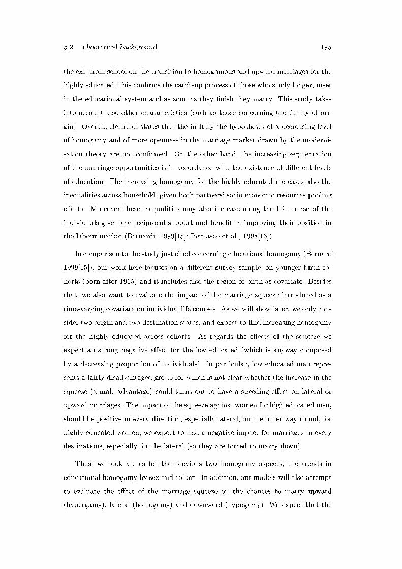
5.2. Theoretical background 195
the exit from school on the transition to homogamous and upward marriages for the
highly educated: this con�rms the catch-up process of those who study longer, meet
in the educational system and as soon as they �nish they marry. This study takes
into account also other characteristics (such as those concerning the family of ori-
gin). Overall, Bernardi states that the in Italy the hypotheses of a decreasing level
of homogamy and of more openness in the marriage market drawn by the moderni-
sation theory are not con�rmed. On the other hand, the increasing segmentation
of the marriage opportunities is in accordance with the existence of di�erent levels
of education. The increasing homogamy for the highly educated increases also the
inequalities across household, given both partners' socio-economic resources pooling
e�ects. Moreover these inequalities may also increase along the life course of the
individuals given the reciprocal support and bene�t in improving their position in
the labour market (Bernardi, 1999[15]; Bernasco et al., 1998[16]).
In comparison to the study just cited concerning educational homogamy (Bernardi,
1999[15]), our work here focuses on a di�erent survey sample, on younger birth co-
horts (born after 1955) and it includes also the region of birth as covariate. Besides
that, we also want to evaluate the impact of the marriage squeeze introduced as a
time-varying covariate on individual life courses. As we will show later, we only con-
sider two origin and two destination states, and expect to �nd increasing homogamy
for the highly educated across cohorts. As regards the e�ects of the squeeze we
expect an strong negative e�ect for the low educated (which is anyway composed
by a decreasing proportion of individuals). In particular, low educated men repre-
sents a fairly disadvantaged group for which is not clear whether the increase in the
squeeze (a male advantage) could turns out to have a speeding e�ect on lateral or
upward marriages. The impact of the squeeze against women for high educated men,
should be positive in every direction, especially lateral; on the other way round, for
highly educated women, we expect to �nd a negative impact for marriages in every
destinations, especially for the lateral (so they are forced to marry down).
Thus, we look at, as for the previous two homogamy aspects, the trends in
educational homogamy by sex and cohort. In addition, our models will also attempt
to evaluate the e�ect of the marriage squeeze on the chances to marry upward
(hypergamy), lateral (homogamy) and downward (hypogamy). We expect that the
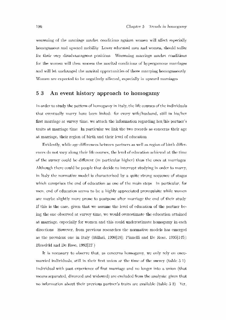
196 Chapter 5. Trends in homogamy
worsening of the marriage market conditions against women will a�ect especially
homogamous and upward mobility. Lower educated men and women, should su�er
for their very disadvantageous positions. Worsening marriage market conditions
for the women will then worsen the marital conditions of hypergamous marriages
and will let unchanged the marital opportunities of those marrying homogamously.
Women are expected to be negatively a�ected, especially in upward marriages.
5.3 An event history approach to homogamy
In order to study the pattern of homogamy in Italy, the life courses of the individuals
that eventually marry have been linked: for every wife/husband, still in his/her
�rst marriage at survey time, we attach the information regarding her/his partner's
traits at marriage time. In particular we link the two records as concerns their age
at marriage, their region of birth and their level of education.
Evidently, while age di�erences between partners as well as region of birth di�er-
ences do not vary along their life courses, the level of education achieved at the time
of the survey could be di�erent (in particular higher) than the ones at marriages.
Although there could be people that decide to interrupt studying in order to marry,
in Italy the normative model is characterised by a quite strong sequence of stages
which comprises the end of education as one of the main steps. In particular, for
men, end of education seems to be a highly appreciated prerequisite while women
are maybe slightly more prone to postpone after marriage the end of their study.
If this is the case, given that we assume the level of education of the partner be-
ing the one observed at survey time, we would overestimate the education attained
at marriage, especially for women and this could underestimate homogamy in each
directions. However, from previous researches the normative models has emerged
as the prevalent one in Italy (Billari, 1998[18]; Pinnelli and De Rose, 1995[145];
Blossfeld and De Rose, 1992[22]).
It is necessary to observe that, as concerns homogamy, we only rely on once-
married individuals, still in their �rst union at the time of the survey (table 5.1).
Individual with past experience of �rst marriage and no longer into a union (that
means separated, divorced and widowed) are excluded from the analysis: given that
no information about their previous partner's traits are available (table 5.2). Yet,
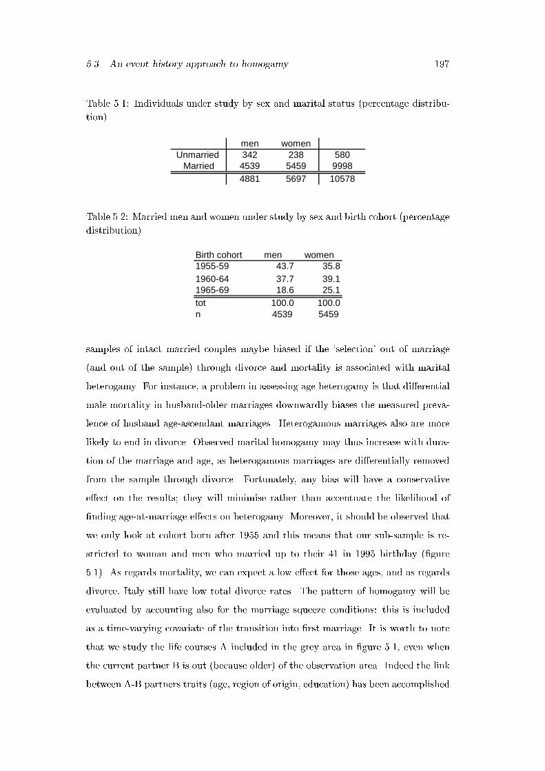
5.3. An event history approach to homogamy 197
Table 5.1: Individuals under study by sex and marital status (percentage distribu-
tion)
men womenUnmarried 342 238 580
Married 4539 5459 99984881 5697 10578
Table 5.2: Married men and women under study by sex and birth cohort (percentage
distribution)
Birth cohort men women1955-59 43.7 35.81960-64 37.7 39.11965-69 18.6 25.1tot 100.0 100.0n 4539 5459
samples of intact married couples maybe biased if the `selection' out of marriage
(and out of the sample) through divorce and mortality is associated with marital
heterogamy. For instance, a problem in assessing age heterogamy is that di�erential
male mortality in husband-older marriages downwardly biases the measured preva-
lence of husband age-ascendant marriages. Heterogamous marriages also are more
likely to end in divorce. Observed marital homogamy may thus increase with dura-
tion of the marriage and age, as heterogamous marriages are di�erentially removed
from the sample through divorce. Fortunately, any bias will have a conservative
e�ect on the results; they will minimise rather than accentuate the likelihood of
�nding age-at-marriage e�ects on heterogamy. Moreover, it should be observed that
we only look at cohort born after 1955 and this means that our sub-sample is re-
stricted to woman and men who married up to their 41 in 1995 birthday (�gure
5.1). As regards mortality, we can expect a low e�ect for those ages, and as regards
divorce, Italy still have low total divorce rates. The pattern of homogamy will be
evaluated by accounting also for the marriage squeeze conditions: this is included
as a time-varying covariate of the transition into �rst marriage. It is worth to note
that we study the life courses A included in the grey area in �gure 5.1, even when
the current partner B is out (because older) of the observation area. Indeed the link
between A-B partners traits (age, region of origin, education) has been accomplished

198 Chapter 5. Trends in homogamy
Figure 5.1: Linkage between partners' traits on the observation area
Age50
48
46
44
42
40
38
36
34
32
30
28
26
24
22
20
18
16
14
birth cohort 1955 birth cohort 1980 12
10
8
6
4
2
0
1st January 1969 1971 1973 1975 1977 1979 1981 1983 1985 1987 1989 1991 1993 1995 1997 1999 Time
June 1998 - SURVEY
B
A
A and B are partners that marry in a given point in time. Their life-courses are linked at
the time of their marriage. Only A will be include in the analysis, as s/he belongs to the
grey area for which we have the possibility to include the squeeze e�ect. Thus A maintains
the information concerning age, region of birth, level of education of the partner B.
5.3. An event history approach to homogamy 199
before selecting for the cohort born after 1955 and younger than 41 in 1995.
Then the analysis is conducted in two steps. The �rst provides a description by
sex and birth cohorts of the homogamy pattern by using the Nelson-Aalen estimator
of the integrated hazard function. The second part of the analysis aims at modeling
the transition rates to the alternative destinations by sex. The covariates we are
going to include in the models are: birth cohort (only the cohorts 1955-59, 1960-64
and 1965-69 are included), region of birth, and a time-varying covariate expressing
the conditions of the marriage market.
The destinations that we consider depend on the type of homogamy we are study-
ing. To exemplify, in �gure 5.2 we report the sketch of the multiple destinations we
are going to present here. Each individual A will have the opportunity to marry
B in one of the alternative destinations, according to its origin state. In �gure 5.2
we exemplify the multiple possible destinations that A is going to face. As we can
see in studying age homogamy between partners we calculate the age di�erence for
those married (in months) and we distinguish among three possible destinations.
Age is a continuous variable, and we assume that one can always marry someone
older/younger than her/himself; therefore we leave open the upward and the down-
ward age interval. In this way we allow for the 3 alternative destinations: marrying
upward (the partner is older: hypergamy), lateral (the partner is about the same
age; homogamy) and downward (the partner is younger: hypogamy). Age homog-
amous couples are here de�ned as those where the age di�erence among partner
is such that she is older than him of at most one year or he is older than her of
2 years. The second case (�gure 5.2) consists in studying by homogamy place of
origin: here we look at the region of birth of both partners. Region of birth is a
qualitative variable. Here we have that each individual can either marry a parter
born in the same region (homogamy) or marry a partner coming from a di�erent
place of birth (heterogamy). Of course, we exclude all respondents who are born
abroad. Lastly, our concern is in studying homogamy by educational attainment.
Apart from the lack of information concerning the year of end of studying, another
crucial problem rises in adopting a particular classi�cation of education. Given that
the level of education attained distinguishes individuals along a ladder, it is relevant
to consider the step where one is located. Table 5.3 reports men and women in their
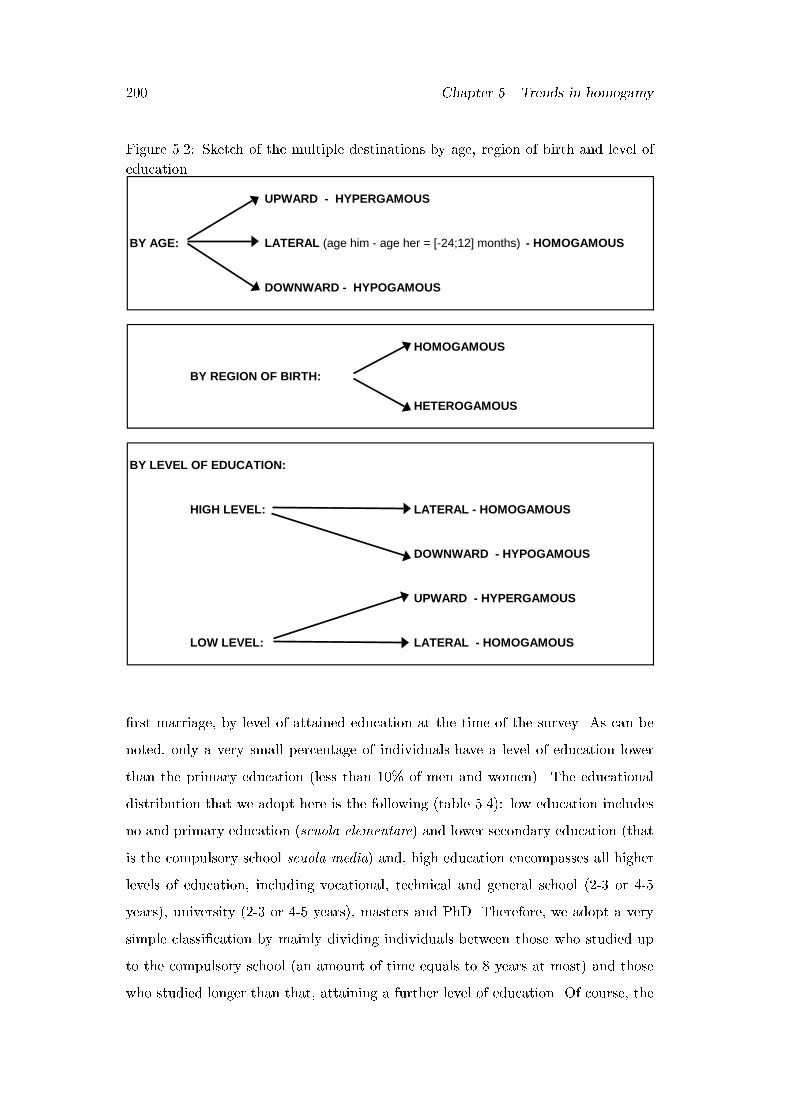
200 Chapter 5. Trends in homogamy
Figure 5.2: Sketch of the multiple destinations by age, region of birth and level of
education
UPWARD - HYPERGAMOUS
BY AGE: LATERAL (age him - age her = [-24;12] months) - HOMOGAMOUS
DOWNWARD - HYPOGAMOUS
HOMOGAMOUS
BY REGION OF BIRTH:
HETEROGAMOUS
BY LEVEL OF EDUCATION:
HIGH LEVEL: LATERAL - HOMOGAMOUS
DOWNWARD - HYPOGAMOUS
UPWARD - HYPERGAMOUS
LOW LEVEL: LATERAL - HOMOGAMOUS
�rst marriage, by level of attained education at the time of the survey. As can be
noted, only a very small percentage of individuals have a level of education lower
than the primary education (less than 10% of men and women). The educational
distribution that we adopt here is the following (table 5.4): low education includes
no and primary education (scuola elementare) and lower secondary education (that
is the compulsory school scuola media) and, high education encompasses all higher
levels of education, including vocational, technical and general school (2-3 or 4-5
years), university (2-3 or 4-5 years), masters and PhD. Therefore, we adopt a very
simple classi�cation by mainly dividing individuals between those who studied up
to the compulsory school (an amount of time equals to 8 years at most) and those
who studied longer than that, attaining a further level of education. Of course, the
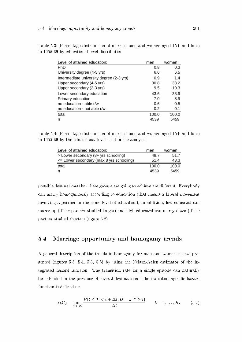
5.4. Marriage opportunity and homogamy trends 201
Table 5.3: Percentage distribution of married men and women aged 15+ and born
in 1955-69 by educational level distribution
Level of attained education: men womenPhD 0.8 0.3University degree (4-5 yrs) 6.6 6.5Intermediate university degree (2-3 yrs) 0.9 1.4Upper secondary (4-5 yrs) 30.8 33.2Upper secondary (2-3 yrs) 9.5 10.3Lower secondary education 43.6 38.9Primary education 7.0 8.9no education - able r/w 0.6 0.5no education - not able r/w 0.2 0.1total 100.0 100.0n 4539 5459
Table 5.4: Percentage distribution of married men and women aged 15+ and born
in 1955-69 by the educational level used in the analysis
Level of attained education: men women> Lower secondary (8+ yrs schooling) 48.7 51.7<= Lower secondary (max 8 yrs schooling) 51.4 48.3total 100.0 100.0n 4539 5459
possible destinations that these groups are going to achieve are di�erent. Everybody
can marry homogamously according to education (that means a lateral movement
involving a partner in the same level of education); in addition, low educated can
marry up (if the partner studied longer) and high educated can marry down (if the
partner studied shorter) (�gure 5.2).
5.4 Marriage opportunity and homogamy trends
A general description of the trends in homogamy for men and women is here pre-
sented (�gures 5.3, 5.4, 5.5, 5.6) by using the Nelson-Aalen estimator of the in-
tegrated hazard function. The transition rate for a single episode can naturally
be extended in the presence of several destinations. The transition-speci�c hazard
function is de�ned as:
rk(t) = lim�t!0
P (t � T < t+�t;D = kjT � t)
�tk = 1; : : : ;K: (5.1)
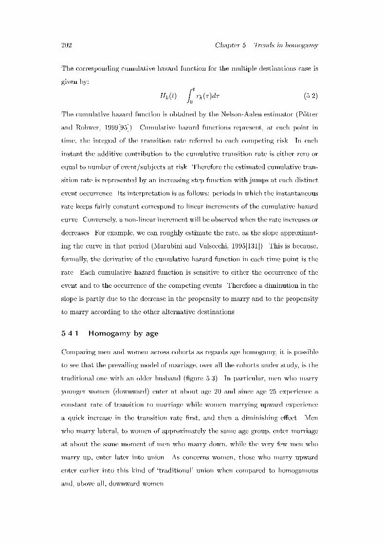
202 Chapter 5. Trends in homogamy
The corresponding cumulative hazard function for the multiple destinations case is
given by:
Hk(t) =
Z t
0rk(�)d� (5.2)
The cumulative hazard function is obtained by the Nelson-Aalen estimator (P�otter
and Rohwer, 1999[95]). Cumulative hazard functions represent, at each point in
time, the integral of the transition rate referred to each competing risk. In each
instant the additive contribution to the cumulative transition rate is either zero or
equal to number of event/subjects at risk. Therefore the estimated cumulative tran-
sition rate is represented by an increasing step function with jumps at each distinct
event occurrence. Its interpretation is as follows: periods in which the instantaneous
rate keeps fairly constant correspond to linear increments of the cumulative hazard
curve. Conversely, a non-linear increment will be observed when the rate increases or
decreases. For example, we can roughly estimate the rate, as the slope approximat-
ing the curve in that period (Marubini and Valsecchi, 1995[131]). This is because,
formally, the derivative of the cumulative hazard function in each time point is the
rate. Each cumulative hazard function is sensitive to either the occurrence of the
event and to the occurrence of the competing events. Therefore a diminution in the
slope is partly due to the decrease in the propensity to marry and to the propensity
to marry according to the other alternative destinations.
5.4.1 Homogamy by age
Comparing men and women across cohorts as regards age homogamy, it is possible
to see that the prevailing model of marriage, over all the cohorts under study, is the
traditional one with an older husband (�gure 5.3). In particular, men who marry
younger women (downward) enter at about age 20 and since age 25 experience a
constant rate of transition to marriage while women marrying upward experience
a quick increase in the transition rate �rst, and then a diminishing e�ect. Men
who marry lateral, to women of approximately the same age group, enter marriage
at about the same moment of men who marry down, while the very few men who
marry up, enter later into union. As concerns women, those who marry upward
enter earlier into this kind of `traditional' union when compared to homogamous
and, above all, downward women.
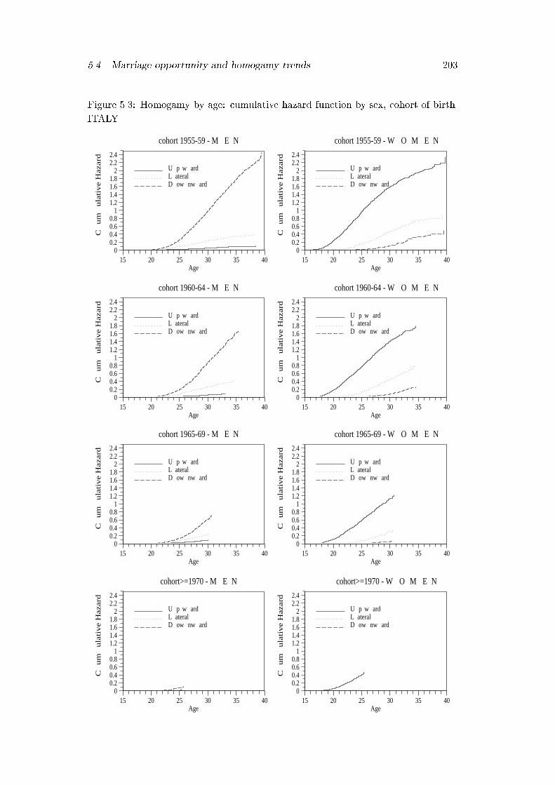
5.4. Marriage opportunity and homogamy trends 203
Figure 5.3: Homogamy by age: cumulative hazard function by sex, cohort of birth.
ITALY
15 20 25 30 35 400
0.20.40.60.8
11.21.41.61.8
22.22.4
cohort>=1970 - M E N
Age
Cum
ula
tive
Haz
ard
U p w ardL ateralD ow nw ard
15 20 25 30 35 400
0.20.40.60.8
11.21.41.61.8
22.22.4
cohort>=1970 - W O M E N
Age
Cum
ula
tive
Haz
ard
U p w ardL ateralD ow nw ard
15 20 25 30 35 400
0.20.40.60.8
11.21.41.61.8
22.22.4
cohort 1965-69 - M E N
Age
Cum
ula
tive
Haz
ard
U p w ardL ateralD ow nw ard
15 20 25 30 35 400
0.20.40.60.8
11.21.41.61.8
22.22.4
cohort 1965-69 - W O M E N
Age
Cum
ula
tive
Haz
ard
U p w ardL ateralD ow nw ard
15 20 25 30 35 400
0.20.40.60.8
11.21.41.61.8
22.22.4
cohort 1960-64 - M E N
Age
Cum
ula
tive
Haz
ard
U p w ardL ateralD ow nw ard
15 20 25 30 35 400
0.20.40.60.8
11.21.41.61.8
22.22.4
cohort 1960-64 - W O M E N
Age
Cum
ula
tive
Haz
ard
U p w ardL ateralD ow nw ard
15 20 25 30 35 400
0.20.40.60.8
11.21.41.61.8
22.22.4
cohort 1955-59 - M E N
Age
Cum
ula
tive
Haz
ard
U p w ardL ateralD ow nw ard
15 20 25 30 35 400
0.20.40.60.8
11.21.41.61.8
22.22.4
cohort 1955-59 - W O M E N
Age
Cum
ula
tive
Haz
ard
U p w ardL ateralD ow nw ard

204 Chapter 5. Trends in homogamy
When we look at the dynamics across cohorts we note that the cumulative hazard
rate for the downward movement of men at age 30 decreased from 0.98 for the 1955-
59 cohort, to 0.88 for the 1960-64 cohort and down to 0.62 for the 1965-69 cohort.
This decrease is also accompanied by a slight increase of the upward movement:
the integral of the transition rate to wife-older marriages passed from 0.06 for the
oldest cohort to 0.10 for the cohort 1965-69. This means a relative decrease of the
transition rate for the traditional downward age destination and a slight increase
of the `atypical' mates characterised by women older than their men. As regards
women, it worth noting that lateral transitions occur later than upward ones and,
again, downward movements occur even later than the lateral ones. This is because
women who marry young re ect the preference for an age gap with the partner larger
than 2 years, while older women are more prone to marry men of approximately the
same age or even younger. While for men we could notice an increase in upward
marriages across cohorts, it is not possible to say much about women who marry
down: in order to see this, we need them to become older so to include younger men.
Indeed, it is also interesting to note the shift in the cumulative hazard for downward
marriages around age 33, for the oldest cohort of women (born in 1955-59). The step
suggests that there was a sudden increase in the downward transition rate. Caution
should be used in assessing an increment in the proportion of those experiencing
marriage, because when the exposed to risk are relatively few, the occurrence of
small number of events may be magni�ed in the graphical representation of the
rate.
5.4.2 Homogamy by place of origin
Let us now look at the dynamics of homogamy by place of origin. The graphs are
reported in �gure 5.4. Men and women marry more often someone coming from the
same region of birth: the cumulative hazards, of homogamous marriages is linearly
increasing for both sexes, meaning a constant rate of transition to �rst marriage to
a partner born in the same region. At age 30 the homogamous cumulative hazards
declines over the cohorts: for men born in 1955-59 it is 0.97, then it reaches 0.94
for the birth cohort 1960-64 and 0.71 for those born in 1965-69. In the same way
the cumulative rate for homogamous marriages for women is around 1.7 for those
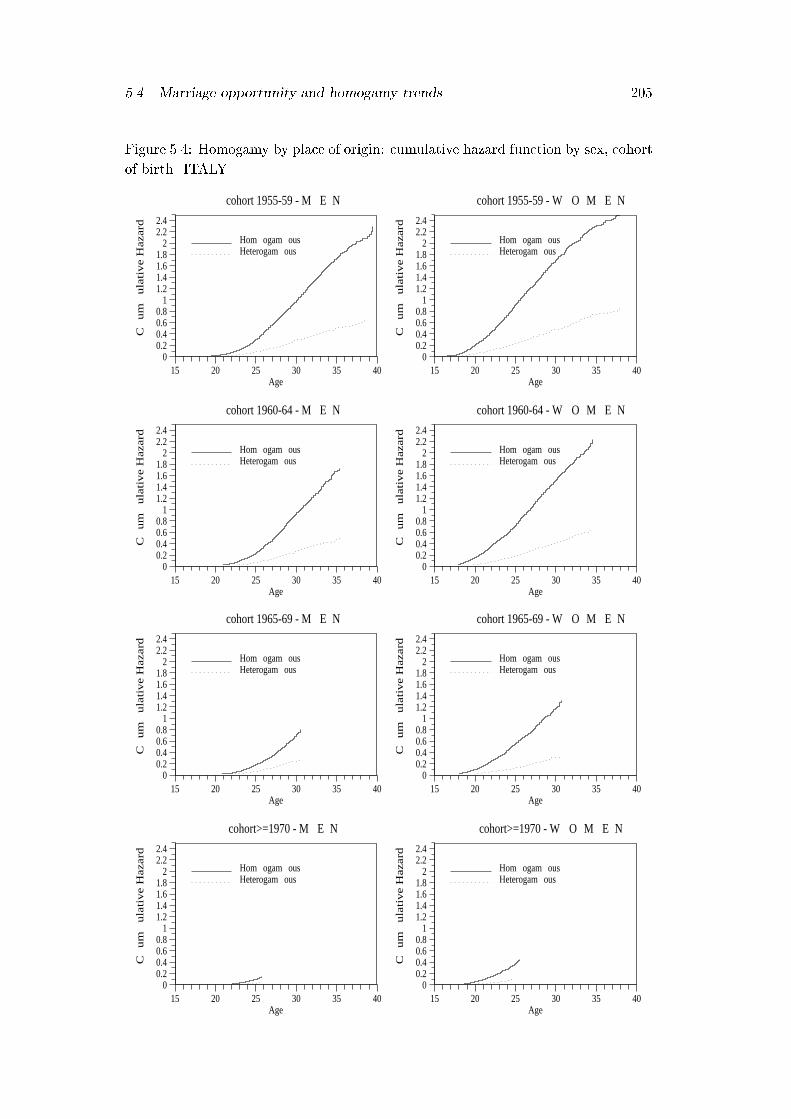
5.4. Marriage opportunity and homogamy trends 205
Figure 5.4: Homogamy by place of origin: cumulative hazard function by sex, cohort
of birth. ITALY
15 20 25 30 35 400
0.20.40.60.8
11.21.41.61.8
22.22.4
cohort>=1970 - M E N
Age
Cum
ula
tive
Haz
ard
Hom ogam ousHeterogam ous
15 20 25 30 35 400
0.20.40.60.8
11.21.41.61.8
22.22.4
cohort>=1970 - W O M E N
Age
Cum
ula
tive
Haz
ard
Hom ogam ousHeterogam ous
15 20 25 30 35 400
0.20.40.60.8
11.21.41.61.8
22.22.4
cohort 1965-69 - M E N
Age
Cum
ula
tive
Haz
ard
Hom ogam ousHeterogam ous
15 20 25 30 35 400
0.20.40.60.8
11.21.41.61.8
22.22.4
cohort 1965-69 - W O M E N
Age
Cum
ula
tive
Haz
ard
Hom ogam ousHeterogam ous
15 20 25 30 35 400
0.20.40.60.8
11.21.41.61.8
22.22.4
cohort 1960-64 - M E N
Age
Cum
ula
tive
Haz
ard
Hom ogam ousHeterogam ous
15 20 25 30 35 400
0.20.40.60.8
11.21.41.61.8
22.22.4
cohort 1960-64 - W O M E N
Age
Cum
ula
tive
Haz
ard
Hom ogam ousHeterogam ous
15 20 25 30 35 400
0.20.40.60.8
11.21.41.61.8
22.22.4
cohort 1955-59 - M E N
Age
Cum
ula
tive
Haz
ard
Hom ogam ousHeterogam ous
15 20 25 30 35 400
0.20.40.60.8
11.21.41.61.8
22.22.4
cohort 1955-59 - W O M E N
Age
Cum
ula
tive
Haz
ard
Hom ogam ousHeterogam ous
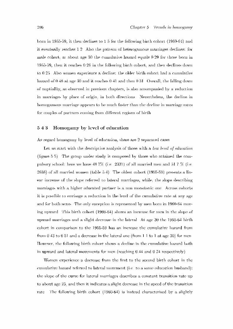
206 Chapter 5. Trends in homogamy
born in 1955-59, it then declines to 1.5 for the following birth cohort (1960-64) and
it eventually reaches 1.2. Also the pattern of heterogamous marriages declines: for
male cohort, at about age 30 the cumulative hazard equals 0.29 for those born in
1955-59, then it reaches 0.26 in the following birth cohort, and then declines down
to 0.25. Also women experience a decline: the older birth cohort had a cumulative
hazard of 0.48 at age 30 and it reaches 0.41 and then 0.31. Overall, the falling down
of nuptiality, as observed in previous chapters, is also accompanied by a reduction
in marriages by place of origin, in both directions. Nevertheless, the decline in
homogamous marriage appears to be much faster than the decline in marriage rates
for couples of partners coming from di�erent regions of birth.
5.4.3 Homogamy by level of education
As regard homogamy by level of education, there are 2 separated cases.
Let us start with the descriptive analysis of those with a low level of education
(�gure 5.5). The group under study is composed by those who attained the com-
pulsory school: here we have 48.7% (i.e. 2331) of all married men and 51.7 % (i.e.
2638) of all married women (table 5.4). The oldest cohort (1955-59) presents a lin-
ear increase of the slope referred to lateral marriages, while, the slope describing
marriages with a higher educated partner is a non-monotonic one. Across cohorts
it is possible to envisage a reduction in the level of the cumulative rate at any age
and for both sexes. The only exception is represented by men born in 1960-64 mov-
ing upward. This birth cohort (1960-64) shows an increase for men in the slope of
upward marriages and a slight decrease in the lateral. At age 30 the 1960-64 birth
cohort in comparison to the 1955-59 has an increase the cumulative hazard from
from 0.43 to 0.51 and a decrease in the lateral one (from 1.1 to 1 at age 30) for men.
However, the following birth cohort shows a decline in the cumulative hazard both
in upward and lateral movements for men (reaching 0.44 and 0.74 respectively).
Women experience a decrease from the �rst to the second birth cohort in the
cumulative hazard referred to lateral movement (i.e. to a same education husband):
the slope of the curve for lateral marriages describes a constant transition rate up
to about age 25, and then it indicates a slight decrease in the speed of the transition
rate. The following birth cohort (1960-64) is instead characterised by a slightly
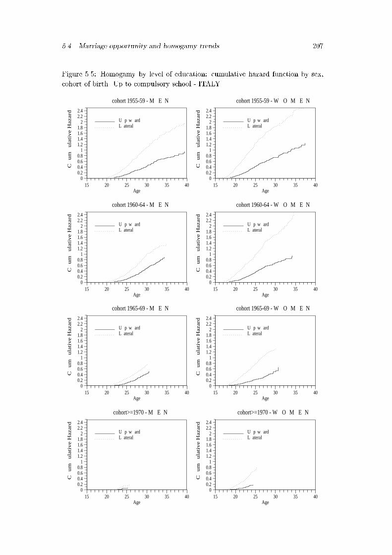
5.4. Marriage opportunity and homogamy trends 207
Figure 5.5: Homogamy by level of education: cumulative hazard function by sex,
cohort of birth. Up to compulsory school - ITALY
15 20 25 30 35 400
0.20.40.60.8
11.21.41.61.8
22.22.4
cohort>=1970 - M E N
Age
Cum
ula
tive
Haz
ard
U p w ardL ateral
15 20 25 30 35 400
0.20.40.60.8
11.21.41.61.8
22.22.4
cohort>=1970 - W O M E N
Age
Cum
ula
tive
Haz
ard
U p w ardL ateral
15 20 25 30 35 400
0.20.40.60.8
11.21.41.61.8
22.22.4
cohort 1965-69 - M E N
Age
Cum
ula
tive
Haz
ard
U p w ardL ateral
15 20 25 30 35 400
0.20.40.60.8
11.21.41.61.8
22.22.4
cohort 1965-69 - W O M E N
Age
Cum
ula
tive
Haz
ard
U p w ardL ateral
15 20 25 30 35 400
0.20.40.60.8
11.21.41.61.8
22.22.4
cohort 1960-64 - M E N
Age
Cum
ula
tive
Haz
ard
U p w ardL ateral
15 20 25 30 35 400
0.20.40.60.8
11.21.41.61.8
22.22.4
cohort 1960-64 - W O M E N
Age
Cum
ula
tive
Haz
ard
U p w ardL ateral
15 20 25 30 35 400
0.20.40.60.8
11.21.41.61.8
22.22.4
cohort 1955-59 - M E N
Age
Cum
ula
tive
Haz
ard
U p w ardL ateral
15 20 25 30 35 400
0.20.40.60.8
11.21.41.61.8
22.22.4
cohort 1955-59 - W O M E N
AgeC
um
ula
tive
Haz
ard
U p w ardL ateral

208 Chapter 5. Trends in homogamy
faster transition to �rst marriage to men with the same educational attainment
starting from age 18. However, at age 30 the level of the cumulative hazard for
lateral marriages is 1.84, 1.69 and 1.28 for the birth cohort 1955-59, 1960-64 and
1965-69 respectively. In the same way also the slope of the curve referred to upward
marriages decreases over time: it is about 0.73 at age 30 for the 1955-59 cohort and
it falls to 0.68 and 0.50 for the birth cohort 1-60-64 and 1965-69 respectively.
The second group of analysis is composed by those with high education: here
there are 51% of married men and 48.3 % of married women (table 5.4). They face
the possibility to marry someone with the same or lower level of education. Despite
the reduction of the level of the curves across cohorts, homogamous couples with
high education prevail. At age 30 the cumulative hazards has declined for men,
from 0.81 for the 1955-59 cohort to 0.76 for the 1960-64 cohort, down to 0.57 for
the 1965-69. Female cumulative hazards for lateral movements has declined as well
from 1.43 to 1.22, down to 0.89. However it should be observed that the deepest
reduction of the curve, occurring between the second and the third cohort for men
in lateral movements, is also accompanied by a small reduction of the in the curve
referred to downward marriages. Downward marriages have declined less, considered
that the cumulative hazards for women have decreased a little from the birth cohort
1955-59 (0.46) to the birth cohort 1960-64 (0.44). It is worth to note, that to observe
downward marriages for women it is necessary to have a longer period of observation.
We can argue an increasing pattern but it can not be said much more at the moment.
Overall, for highly educated, a reduction of the slope towards lateral and down-
ward marriages can be envisaged across cohorts, even though downward marriages
show a slow down for both sexes.
5.5 Modeling homogamy
As we already said in the introduction to this chapter, our second step consists in
studying the pattern of homogamy and its dynamics by using semi-parametric event
history models. This implies modeling the destination-speci�c hazard as a function
of a covariates vector: X1 for the birth cohort (with dummy coding), X2 for the
region of birth (with dummy coding) and X3 for the marriage market conditions

5.5. Modeling homogamy 209
Figure 5.6: Homogamy by level of education: cumulative hazard function by sex,
cohort of birth. Higher than compulsory school - ITALY
15 20 25 30 35 400
0.20.40.60.8
11.21.41.61.8
22.22.4
cohort>=1970 - M E N
Age
Cum
ula
tive
Haz
ard
L ateralD ow nw ard
15 20 25 30 35 400
0.20.40.60.8
11.21.41.61.8
22.22.4
cohort>=1970 - W O M E N
Age
Cum
ula
tive
Haz
ard
L ateralD ow nw ard
15 20 25 30 35 400
0.20.40.60.8
11.21.41.61.8
22.22.4
cohort 1965-69 - M E N
Age
Cum
ula
tive
Haz
ard
L ateralD ow nw ard
15 20 25 30 35 400
0.20.40.60.8
11.21.41.61.8
22.22.4
cohort 1965-69 - W O M E N
Age
Cum
ula
tive
Haz
ard
L ateralD ow nw ard
15 20 25 30 35 400
0.20.40.60.8
11.21.41.61.8
22.22.4
cohort 1960-64 - M E N
Age
Cum
ula
tive
Haz
ard
L ateralD ow nw ard
15 20 25 30 35 400
0.20.40.60.8
11.21.41.61.8
22.22.4
cohort 1960-64 - W O M E N
Age
Cum
ula
tive
Haz
ard
L ateralD ow nw ard
15 20 25 30 35 400
0.20.40.60.8
11.21.41.61.8
22.22.4
cohort 1955-59 - M E N
Age
Cum
ula
tive
Haz
ard
L ateralD ow nw ard
15 20 25 30 35 400
0.20.40.60.8
11.21.41.61.8
22.22.4
cohort 1955-59 - W O M E N
AgeC
um
ula
tive
Haz
ard
L ateralD ow nw ard

210 Chapter 5. Trends in homogamy
(unidimensional value as a continuous variable):
rk(t) = r0k(t) exp(�1kX1 + �2kX2 + �3kX3) (5.3)
This is a straightforward extension of single transition semi-parametric model used
in the previous chapter; however it is worth noting that both the baseline r0k and
the vector of regression coe�cients �ik are now speci�c to each destination. The
baseline function is the the hazard function of an individual with all covariates of
value zero and in this case is referred to an individual born in 1955-59, in Piedmont
and in a balanced marriage market. Following the sketch given in �gure 5.2 we
perform multiple destination models on the rate of marrying a partner with given
traits. The case of educational homogamy will need to distinguish, as we did in the
descriptive analysis, two di�erent models each of them referred to the same set of
individuals.
The approach that we follow is fairly new in the panorama of the techniques
of analysis used in studying homogamy. Recently, event history analysis has been
applied in particular to study homogamy by educational level, but less attention
has been paid to the dynamics of age and place of origin homogamy. As far as the
review of the literature we presented is concerned, we note that only few attempts
have been made to include a compositional factor in the analysis of homogamy. In
our case, it represents the yearly imbalances of the marriage market of the region
where individuals were born.
5.5.1 Homogamy by age
In section 5.3 we said that, to compare partners' age, we have that each individual
may marry in one of the three possible destinations: i.e. s/he can marry a older
(upward), same-age (lateral) or younger (downward) partner. Focusing on the birth
cohorts born between 1955 and 1965, table 5.5 summarises the frequencies for each
direction of age homogamy by sex: it emerges that, for women, the proportion of
hypergamous marriage declines a little bit and then it rises; for men, either ho-
mogamous and hypergamous marriages have increased. The distribution of the age
di�erences for men and for women is reported in �gures 5.7 and 5.8: the frequency
of marriages with lower age di�erence rises. The age-partner di�erence over time
appears more stable when we look at women. We should note that the di�erence
5.5. Modeling homogamy 211
Figure 5.7: Age di�erences between partners; by married men, cohorts 1955-69 -
ITALY
0
2
4
6
8
10
12
14
16
18
-18 -13 -8 -3 2 7 12 17 22 27
age difference: women-men
per
cen
tag
e 1955-59
1960-64
1965-69
between the two cases is due to the fact that, if we select married individuals born
in the cohort 1955-69, we observe a slightly higher frequency of married women
(5459) than of married men (4539). Therefore, men much older than their women
are slightly under-represented. In tables 5.6 and 5.7 we report the Cox models for
multiple destinations, with birth cohort and region of birth as covariate (Model 1)
and we add the e�ect of the squeeze in the lower part (Model 2). The measures of
the marriage market (S, I and Ifreq) introduced in the previous chapter have been
used in alternative models, but, as they yield the same results we only present the
outcome referred to the model with the best BIC (Model 2 in all tables di�ers from
Model 1 for the addition of the e�ect of the squeeze). In particular as concerns the
age di�erence between partners the measure of the marriage market conditions here
adopted for men is the one based on S the Schoen index and for women is the one
based on the measure I. For the sake of simplicity, we do not present the estimation
of the Cox models based on the other two measures, but the choice was checked on
the basis of the lowest BIC statistics.
Men born in 1960-64 have almost the same competing risk to marry upward and
lateral as those born a bit earlier (cohort 1955-59): the younger cohort has slightly
slower transition to downward marriages (i.e. to marriage to a younger woman)
than those born in 1955-59 (table 5.6). With respect to the reference cohort (1955-
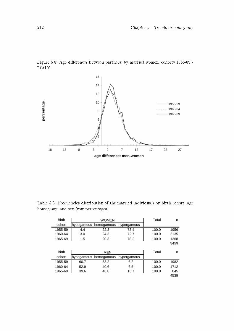
212 Chapter 5. Trends in homogamy
Figure 5.8: Age di�erences between partners; by married women, cohorts 1955-69 -
ITALY
0
2
4
6
8
10
12
14
16
-18 -13 -8 -3 2 7 12 17 22 27
age difference: men-women
per
cen
tag
e
1955-59
1960-64
1965-69
Table 5.5: Frequencies distribution of the married individuals by birth cohort, age
homogamy, and sex (row percentages)
Birth Total ncohort hypogamous homogamous hypergamous
1955-59 4.4 22.3 73.4 100.0 19561960-64 3.0 24.3 72.7 100.0 21351965-69 1.5 20.3 78.2 100.0 1368
5459
Birth Total ncohort hypogamous homogamous hypergamous
1955-59 60.7 33.2 6.2 100.0 19821960-64 52.9 40.6 6.5 100.0 17121965-69 39.6 46.6 13.7 100.0 845
4539
WOMEN
MEN
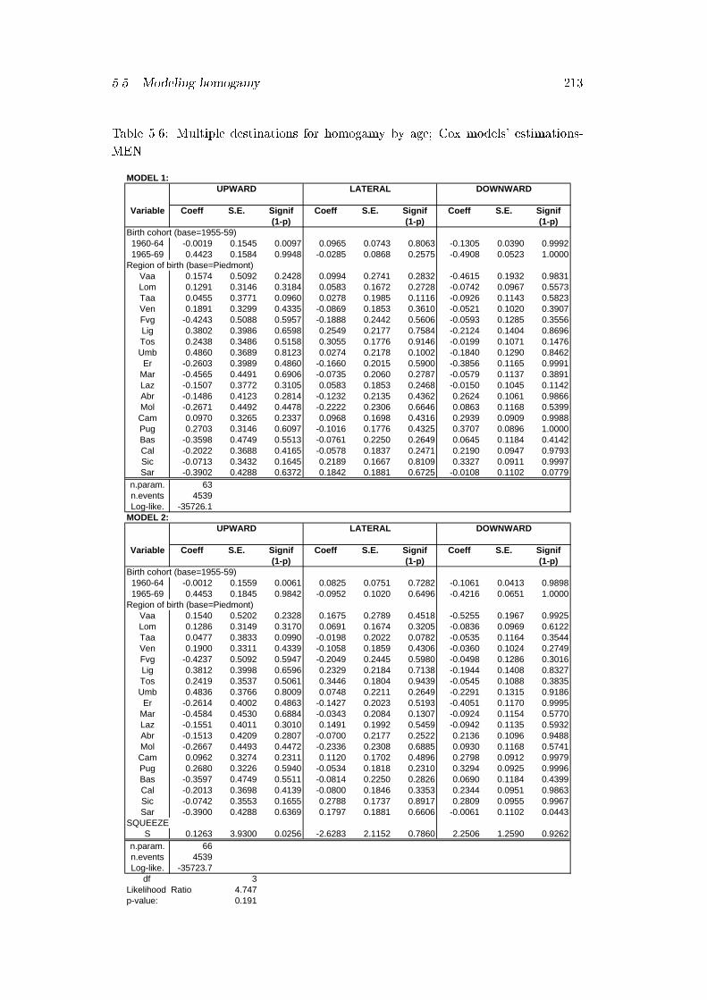
5.5. Modeling homogamy 213
Table 5.6: Multiple destinations for homogamy by age; Cox models' estimations-
MEN
MODEL 1:
Variable Coeff S.E. Signif Coeff S.E. Signif Coeff S.E. Signif(1-p) (1-p) (1-p)
Birth cohort (base=1955-59)1960-64 -0.0019 0.1545 0.0097 0.0965 0.0743 0.8063 -0.1305 0.0390 0.99921965-69 0.4423 0.1584 0.9948 -0.0285 0.0868 0.2575 -0.4908 0.0523 1.0000
Region of birth (base=Piedmont)Vaa 0.1574 0.5092 0.2428 0.0994 0.2741 0.2832 -0.4615 0.1932 0.9831Lom 0.1291 0.3146 0.3184 0.0583 0.1672 0.2728 -0.0742 0.0967 0.5573Taa 0.0455 0.3771 0.0960 0.0278 0.1985 0.1116 -0.0926 0.1143 0.5823Ven 0.1891 0.3299 0.4335 -0.0869 0.1853 0.3610 -0.0521 0.1020 0.3907Fvg -0.4243 0.5088 0.5957 -0.1888 0.2442 0.5606 -0.0593 0.1285 0.3556Lig 0.3802 0.3986 0.6598 0.2549 0.2177 0.7584 -0.2124 0.1404 0.8696Tos 0.2438 0.3486 0.5158 0.3055 0.1776 0.9146 -0.0199 0.1071 0.1476Umb 0.4860 0.3689 0.8123 0.0274 0.2178 0.1002 -0.1840 0.1290 0.8462Er -0.2603 0.3989 0.4860 -0.1660 0.2015 0.5900 -0.3856 0.1165 0.9991
Mar -0.4565 0.4491 0.6906 -0.0735 0.2060 0.2787 -0.0579 0.1137 0.3891Laz -0.1507 0.3772 0.3105 0.0583 0.1853 0.2468 -0.0150 0.1045 0.1142Abr -0.1486 0.4123 0.2814 -0.1232 0.2135 0.4362 0.2624 0.1061 0.9866Mol -0.2671 0.4492 0.4478 -0.2222 0.2306 0.6646 0.0863 0.1168 0.5399Cam 0.0970 0.3265 0.2337 0.0968 0.1698 0.4316 0.2939 0.0909 0.9988Pug 0.2703 0.3146 0.6097 -0.1016 0.1776 0.4325 0.3707 0.0896 1.0000Bas -0.3598 0.4749 0.5513 -0.0761 0.2250 0.2649 0.0645 0.1184 0.4142Cal -0.2022 0.3688 0.4165 -0.0578 0.1837 0.2471 0.2190 0.0947 0.9793Sic -0.0713 0.3432 0.1645 0.2189 0.1667 0.8109 0.3327 0.0911 0.9997Sar -0.3902 0.4288 0.6372 0.1842 0.1881 0.6725 -0.0108 0.1102 0.0779
n.param. 63n.events 4539Log-like. -35726.1
MODEL 2:
Variable Coeff S.E. Signif Coeff S.E. Signif Coeff S.E. Signif(1-p) (1-p) (1-p)
Birth cohort (base=1955-59)1960-64 -0.0012 0.1559 0.0061 0.0825 0.0751 0.7282 -0.1061 0.0413 0.98981965-69 0.4453 0.1845 0.9842 -0.0952 0.1020 0.6496 -0.4216 0.0651 1.0000
Region of birth (base=Piedmont)Vaa 0.1540 0.5202 0.2328 0.1675 0.2789 0.4518 -0.5255 0.1967 0.9925Lom 0.1286 0.3149 0.3170 0.0691 0.1674 0.3205 -0.0836 0.0969 0.6122Taa 0.0477 0.3833 0.0990 -0.0198 0.2022 0.0782 -0.0535 0.1164 0.3544Ven 0.1900 0.3311 0.4339 -0.1058 0.1859 0.4306 -0.0360 0.1024 0.2749Fvg -0.4237 0.5092 0.5947 -0.2049 0.2445 0.5980 -0.0498 0.1286 0.3016Lig 0.3812 0.3998 0.6596 0.2329 0.2184 0.7138 -0.1944 0.1408 0.8327Tos 0.2419 0.3537 0.5061 0.3446 0.1804 0.9439 -0.0545 0.1088 0.3835Umb 0.4836 0.3766 0.8009 0.0748 0.2211 0.2649 -0.2291 0.1315 0.9186Er -0.2614 0.4002 0.4863 -0.1427 0.2023 0.5193 -0.4051 0.1170 0.9995
Mar -0.4584 0.4530 0.6884 -0.0343 0.2084 0.1307 -0.0924 0.1154 0.5770Laz -0.1551 0.4011 0.3010 0.1491 0.1992 0.5459 -0.0942 0.1135 0.5932Abr -0.1513 0.4209 0.2807 -0.0700 0.2177 0.2522 0.2136 0.1096 0.9488Mol -0.2667 0.4493 0.4472 -0.2336 0.2308 0.6885 0.0930 0.1168 0.5741Cam 0.0962 0.3274 0.2311 0.1120 0.1702 0.4896 0.2798 0.0912 0.9979Pug 0.2680 0.3226 0.5940 -0.0534 0.1818 0.2310 0.3294 0.0925 0.9996Bas -0.3597 0.4749 0.5511 -0.0814 0.2250 0.2826 0.0690 0.1184 0.4399Cal -0.2013 0.3698 0.4139 -0.0800 0.1846 0.3353 0.2344 0.0951 0.9863Sic -0.0742 0.3553 0.1655 0.2788 0.1737 0.8917 0.2809 0.0955 0.9967Sar -0.3900 0.4288 0.6369 0.1797 0.1881 0.6606 -0.0061 0.1102 0.0443
SQUEEZES 0.1263 3.9300 0.0256 -2.6283 2.1152 0.7860 2.2506 1.2590 0.9262
n.param. 66n.events 4539Log-like. -35723.7
df 3Likelihood Ratio 4.747p-value: 0.191
UPWARD LATERAL DOWNWARD
UPWARD LATERAL DOWNWARD
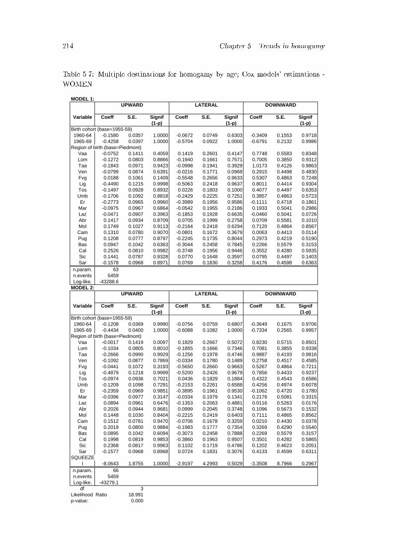
214 Chapter 5. Trends in homogamy
Table 5.7: Multiple destinations for homogamy by age; Cox models' estimations -
WOMEN
MODEL 1:
Variable Coeff S.E. Signif Coeff S.E. Signif Coeff S.E. Signif(1-p) (1-p) (1-p)
Birth cohort (base=1955-59)1960-64 -0.1580 0.0357 1.0000 -0.0672 0.0749 0.6303 -0.3409 0.1553 0.97181965-69 -0.4258 0.0397 1.0000 -0.5704 0.0922 1.0000 -0.6791 0.2132 0.9986
Region of birth (base=Piedmont)Vaa -0.0752 0.1411 0.4059 0.1419 0.2601 0.4147 0.7748 0.5583 0.8348Lom -0.1272 0.0803 0.8866 -0.1940 0.1661 0.7571 0.7005 0.3850 0.9312Taa -0.1843 0.0971 0.9423 -0.0998 0.1941 0.3929 1.0173 0.4126 0.9863Ven -0.0799 0.0874 0.6391 -0.0216 0.1771 0.0969 0.2915 0.4498 0.4830Fvg 0.0188 0.1061 0.1409 -0.5548 0.2656 0.9633 0.5307 0.4863 0.7248Lig -0.4490 0.1215 0.9998 -0.5063 0.2418 0.9637 0.8011 0.4414 0.9304Tos -0.1497 0.0928 0.8932 0.0226 0.1803 0.1000 0.4077 0.4497 0.6353Umb -0.1706 0.1092 0.8818 -0.2429 0.2225 0.7251 0.3857 0.4863 0.5723Er -0.2773 0.0965 0.9960 -0.3989 0.1956 0.9586 -0.1111 0.4718 0.1861
Mar -0.0975 0.0967 0.6864 -0.0542 0.1955 0.2186 0.1933 0.5041 0.2986Laz -0.0471 0.0907 0.3963 -0.1853 0.1928 0.6635 -0.0460 0.5041 0.0726Abr 0.1417 0.0934 0.8709 0.0705 0.1999 0.2758 0.0709 0.5581 0.1010Mol 0.1749 0.1027 0.9113 -0.2164 0.2418 0.6294 0.7120 0.4864 0.8567Cam 0.1310 0.0780 0.9070 -0.0801 0.1672 0.3679 0.0063 0.4413 0.0114Pug 0.1208 0.0777 0.8797 -0.2245 0.1735 0.8044 0.2973 0.4219 0.5190Bas 0.0947 0.1042 0.6363 -0.3044 0.2458 0.7845 0.2266 0.5579 0.3153Cal 0.2526 0.0810 0.9982 -0.3748 0.1956 0.9446 0.3552 0.4280 0.5935Sic 0.1441 0.0787 0.9328 0.0770 0.1648 0.3597 0.0795 0.4497 0.1403Sar -0.1578 0.0968 0.8971 0.0769 0.1830 0.3258 0.4176 0.4598 0.6363
n.param. 63n.events 5459Log-like. -43288.6
MODEL 2:
Variable Coeff S.E. Signif Coeff S.E. Signif Coeff S.E. Signif(1-p) (1-p) (1-p)
Birth cohort (base=1955-59)1960-64 -0.1208 0.0369 0.9990 -0.0756 0.0759 0.6807 -0.3649 0.1675 0.97061965-69 -0.4434 0.0400 1.0000 -0.6088 0.1082 1.0000 -0.7334 0.2565 0.9957
Region of birth (base=Piedmont)Vaa -0.0017 0.1419 0.0097 0.1829 0.2667 0.5072 0.8230 0.5715 0.8501Lom -0.1034 0.0805 0.8010 -0.1855 0.1666 0.7346 0.7081 0.3855 0.9338Taa -0.2666 0.0990 0.9929 -0.1256 0.1978 0.4746 0.9887 0.4193 0.9816Ven -0.1092 0.0877 0.7869 -0.0334 0.1780 0.1489 0.2758 0.4517 0.4585Fvg -0.0441 0.1072 0.3193 -0.5650 0.2660 0.9663 0.5267 0.4864 0.7211Lig -0.4879 0.1218 0.9999 -0.5200 0.2426 0.9679 0.7856 0.4433 0.9237Tos -0.0974 0.0936 0.7021 0.0436 0.1829 0.1884 0.4322 0.4543 0.6586Umb -0.1209 0.1098 0.7291 -0.2153 0.2261 0.6588 0.4256 0.4974 0.6078Er -0.2359 0.0969 0.9851 -0.3895 0.1961 0.9530 -0.1062 0.4720 0.1780
Mar -0.0396 0.0977 0.3147 -0.0334 0.1979 0.1341 0.2176 0.5081 0.3315Laz 0.0894 0.0961 0.6476 -0.1353 0.2063 0.4881 0.0116 0.5263 0.0176Abr 0.2026 0.0944 0.9681 0.0999 0.2045 0.3748 0.1096 0.5673 0.1532Mol 0.1448 0.1030 0.8404 -0.2215 0.2419 0.6403 0.7111 0.4865 0.8562Cam 0.1512 0.0781 0.9470 -0.0706 0.1678 0.3259 0.0210 0.4430 0.0378Pug 0.2019 0.0800 0.9884 -0.1983 0.1777 0.7354 0.3269 0.4290 0.5540Bas 0.0895 0.1042 0.6094 -0.3073 0.2458 0.7888 0.2269 0.5579 0.3157Cal 0.1998 0.0819 0.9853 -0.3860 0.1963 0.9507 0.3501 0.4282 0.5865Sic 0.2368 0.0817 0.9963 0.1102 0.1719 0.4786 0.1202 0.4623 0.2051Sar -0.1577 0.0968 0.8968 0.0724 0.1831 0.3076 0.4133 0.4599 0.6311
SQUEEZEI -8.0643 1.8755 1.0000 -2.9197 4.2993 0.5029 -3.3508 8.7966 0.2967
n.param. 66n.events 5459Log-like. -43279.1
df 3Likelihood Ratio 18.991p-value: 0.000
UPWARD LATERAL DOWNWARD
UPWARD LATERAL DOWNWARD

5.5. Modeling homogamy 215
59), men born in 1965-69 experience a higher transition rate (coe�cient equals to
0.4423 and signi�cant) to marriages to an older woman and a reduction in marriage
transition to a younger woman (the coe�cient is equal to -0.4908 and it is signi�-
cant). This means that, across cohorts, especially from that born in 1965-69, a less
traditional model regarding age di�erence between partners emerges. The relative
decrease of the transition rate for the traditional downward age destination, together
with the slight rise in upward movements, has also emerged earlier in the descrip-
tive analysis based on the cumulative hazard functions (�gure 5.3). Across cohorts,
men experience a change in the model characterising age di�erence in the couple.
Traditionally husband-older couples prevailed. The decrease in the downward rate,
together with the increase in the upward one indicates the existence of a dynam-
ics across cohorts which, for men, moves towards less traditional age-gap between
partners. As concerns the region of birth, a clear distinction between central and
northern regions on one hand with the exception of Piedmont and southern regions
on the other hand emerges: the rate of downward transition is particularly low for
Valle d'Aosta, Liguria, Umbria, Emilia Romagna while it is fairly high in Abruzzo,
Campania, Apulia, Calabria and Sicily (table 5.6). In the same way, upward mar-
riages for men characterise northern regions, con�rming that the traditional custom
of older-husband couple is preferred by men born in the South.
The introduction of the marriage squeeze as a time-varying covariate con�rms the
male advantage in all directions: either downward and upward marriages increase
(even though in the second case the coe�cient is not signi�cant). In particular
the male advantage in the marriage market accelerates downward transitions (the
coe�cient is 2.2506) more than upward marriages (coe�cient is 0.1263). However,
for men the squeeze measure, although yielding the lowest BIC when using the
Schoen index S (with BIC=6.224), does not improve Model 1. As a matter of fact,
the likelihood ratio test makes Model 2 more preferable to Model 1.
As concerns women (table 5.7), the decline in the transition rate to �rst marriage
towards all directions is very strong across cohorts. This reduction is particularly
noticeable in the case of downward marriages, while upward and especially lateral
marriages have declined a little less for women born in 1960-64 in comparison to
those born 5 years earlier. Also the following birth cohort accentuated the same

216 Chapter 5. Trends in homogamy
declining pattern in transition rates. The lowest rate for the birth cohort 1965-69
is the one referred to downward marriages (-0.6791), then to lateral (-0.5704) and
lastly to upward (-0.4258). However, the biggest relative reduction occurs between
the second and the third birth cohort in lateral marriages (to a man of about the
same age): here the rate decreases from -0.0672 for the 1960-64 birth cohort, to
-0.5704 for the 1965-69 birth cohort. In �gure 5.3 we already stressed the deep
decline in the transition rates of the women for every destination, especially for
lateral movements.
Almost all regions of birth have homogamous (lateral) rate lower than Piedmont,
while upward and downward movements highlight the prevailing role of traditional
husband-older couple in the South and the rise in atypical mating in the North
(especially in Trentino Alto Adige, Lombardia, Liguria and Valle d'Aosta, table 5.7).
For women the measure of the squeeze adopted is the index I, with BIC = �7:779.
It is the case to remind that the measure I is obtained by dividing the di�erence
between male and female proportions ever married by their sum. An increase in the
index of the imbalance I reduces the transition rate to �rst marriage for women,
towards all directions. In particular the rate of experiencing an upward marriage
(with an older husband) is lowered more than that for homogamous or downward
marriage. This means that favourable conditions of the marriage market to men may
create a postponement e�ect for women, especially to marry to an older husband.
In sum, men show a shift in the characteristics of the assortative mating model
concerning the age of the spouse. Across cohorts, an increase of upward marriages as
well as a decline of downward marriages have emerged. Conversely for women a shift
from more traditional patterns is not evident, although the youngest cohort shows
a slowing down of the typology of marriage to an older man. Regional di�erences
stress the existence of a traditional model, based on a high age-gap in the South;
in the North, on the contrary, men and women are more prone to age-balanced
relationships.
5.5.2 Homogamy by region of birth
Homogamy by place of origin is studied by distinguishing the possibilities to marry
a partner born in the same region or born somewhere else (�gure 5.2, table 5.8).

5.5. Modeling homogamy 217
Across cohorts there is a reduction in the proportion of heterogamous marriages for
women, and an increase in heterogamous marriages for men. The trend by cohort
Table 5.8: Frequencies distribution of the married individuals by birth cohort, place
of birth homogamy, and sex (row percentages)
Birthcohort homogamous heterogamous Total n
1955-59 78.27 21.73 100 19561960-64 78.92 21.08 100 21351965-69 80.19 19.81 100 1368
5459
Birthcohort homogamous heterogamous Total n
1955-59 77.8 22.2 100 19821960-64 77.39 22.61 100 17121965-69 72.66 27.34 100 845
4539
MEN
WOMEN
reported in the Cox model con�rms a reduction of the marital behaviour for men
(table 5.9). Although men born in 1960-64 have just a slight decline in compari-
son to the previous birth cohort, men born in 1965-69 have a slower transition to
�rst homogamous marriage than the reference group (cohort 1955-59) (coe�cient
=-0.3842) and also a slower transition to heterogamous marriages (-0.1060). Thus,
the decline in the propensity to marry a woman born in the same region is stronger
than the decline in the propensity to marry a woman born in a di�erent region. Tra-
ditional homogamous (by place of origin - endogamous) marriages are more a�ected
by the decline over cohorts than heterogamous marriages.
From table 5.9 it emerges that some regions at the borders of the country or in
a particular position experience a reduction in the rate of outmarriage if compared
to Piedmont: this is the case for Trentino Alto Adige (-0.5984), Valle d'Aosta (-
0.2458), both islands (especially for Sardinia, -0.2708, while Sicily -0.0847), but also
for some other regions on the east coast such as (Marches and Emilia Romagna).
Conversely, being born in Liguria, for instance, determines a higher transition rate
to heterogenous marriages (0.3439): a reason here could be envisaged in the small
size of the population of that region. As we reported in the review of the literature,
it happens that if the group is small but not isolated and it is di�cult to marry
within the group, then it is highly likely to marry outside that group. Moreover
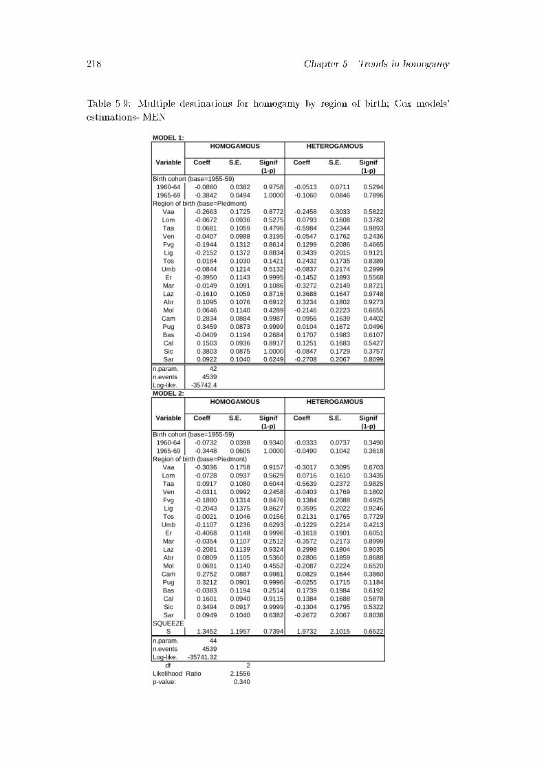
218 Chapter 5. Trends in homogamy
Table 5.9: Multiple destinations for homogamy by region of birth; Cox models'
estimations- MEN
MODEL 1:
Variable Coeff S.E. Signif Coeff S.E. Signif(1-p) (1-p)
Birth cohort (base=1955-59)1960-64 -0.0860 0.0382 0.9758 -0.0513 0.0711 0.52941965-69 -0.3842 0.0494 1.0000 -0.1060 0.0846 0.7896
Region of birth (base=Piedmont)Vaa -0.2663 0.1725 0.8772 -0.2458 0.3033 0.5822Lom -0.0672 0.0936 0.5275 0.0793 0.1608 0.3782Taa 0.0681 0.1059 0.4796 -0.5984 0.2344 0.9893Ven -0.0407 0.0988 0.3195 -0.0547 0.1762 0.2436Fvg -0.1944 0.1312 0.8614 0.1299 0.2086 0.4665Lig -0.2152 0.1372 0.8834 0.3439 0.2015 0.9121Tos 0.0184 0.1030 0.1421 0.2432 0.1735 0.8389Umb -0.0844 0.1214 0.5132 -0.0837 0.2174 0.2999
Er -0.3950 0.1143 0.9995 -0.1452 0.1893 0.5568Mar -0.0149 0.1091 0.1086 -0.3272 0.2149 0.8721Laz -0.1610 0.1059 0.8716 0.3688 0.1647 0.9748Abr 0.1095 0.1076 0.6912 0.3234 0.1802 0.9273Mol 0.0646 0.1140 0.4289 -0.2146 0.2223 0.6655Cam 0.2834 0.0884 0.9987 0.0956 0.1639 0.4402Pug 0.3459 0.0873 0.9999 0.0104 0.1672 0.0496Bas -0.0409 0.1194 0.2684 0.1707 0.1983 0.6107Cal 0.1503 0.0936 0.8917 0.1251 0.1683 0.5427Sic 0.3803 0.0875 1.0000 -0.0847 0.1729 0.3757Sar 0.0922 0.1040 0.6249 -0.2708 0.2067 0.8099
n.param. 42n.events 4539Log-like. -35742.4MODEL 2:
Variable Coeff S.E. Signif Coeff S.E. Signif(1-p) (1-p)
Birth cohort (base=1955-59)1960-64 -0.0732 0.0398 0.9340 -0.0333 0.0737 0.34901965-69 -0.3448 0.0605 1.0000 -0.0490 0.1042 0.3618
Region of birth (base=Piedmont)Vaa -0.3036 0.1758 0.9157 -0.3017 0.3095 0.6703Lom -0.0728 0.0937 0.5629 0.0716 0.1610 0.3435Taa 0.0917 0.1080 0.6044 -0.5639 0.2372 0.9825Ven -0.0311 0.0992 0.2458 -0.0403 0.1769 0.1802Fvg -0.1880 0.1314 0.8476 0.1384 0.2088 0.4925Lig -0.2043 0.1375 0.8627 0.3595 0.2022 0.9246Tos -0.0021 0.1046 0.0156 0.2131 0.1765 0.7729Umb -0.1107 0.1236 0.6293 -0.1229 0.2214 0.4213
Er -0.4068 0.1148 0.9996 -0.1618 0.1901 0.6051Mar -0.0354 0.1107 0.2512 -0.3572 0.2173 0.8999Laz -0.2081 0.1139 0.9324 0.2998 0.1804 0.9035Abr 0.0809 0.1105 0.5360 0.2806 0.1859 0.8688Mol 0.0691 0.1140 0.4552 -0.2087 0.2224 0.6520Cam 0.2752 0.0887 0.9981 0.0829 0.1644 0.3860Pug 0.3212 0.0901 0.9996 -0.0255 0.1715 0.1184Bas -0.0383 0.1194 0.2514 0.1739 0.1984 0.6192Cal 0.1601 0.0940 0.9115 0.1384 0.1688 0.5878Sic 0.3494 0.0917 0.9999 -0.1304 0.1795 0.5322Sar 0.0949 0.1040 0.6382 -0.2672 0.2067 0.8038
SQUEEZES 1.3452 1.1957 0.7394 1.9732 2.1015 0.6522
n.param. 44n.events 4539Log-like. -35741.32
df 2Likelihood Ratio 2.1556p-value: 0.340
HOMOGAMOUS HETEROGAMOUS
HOMOGAMOUS HETEROGAMOUS
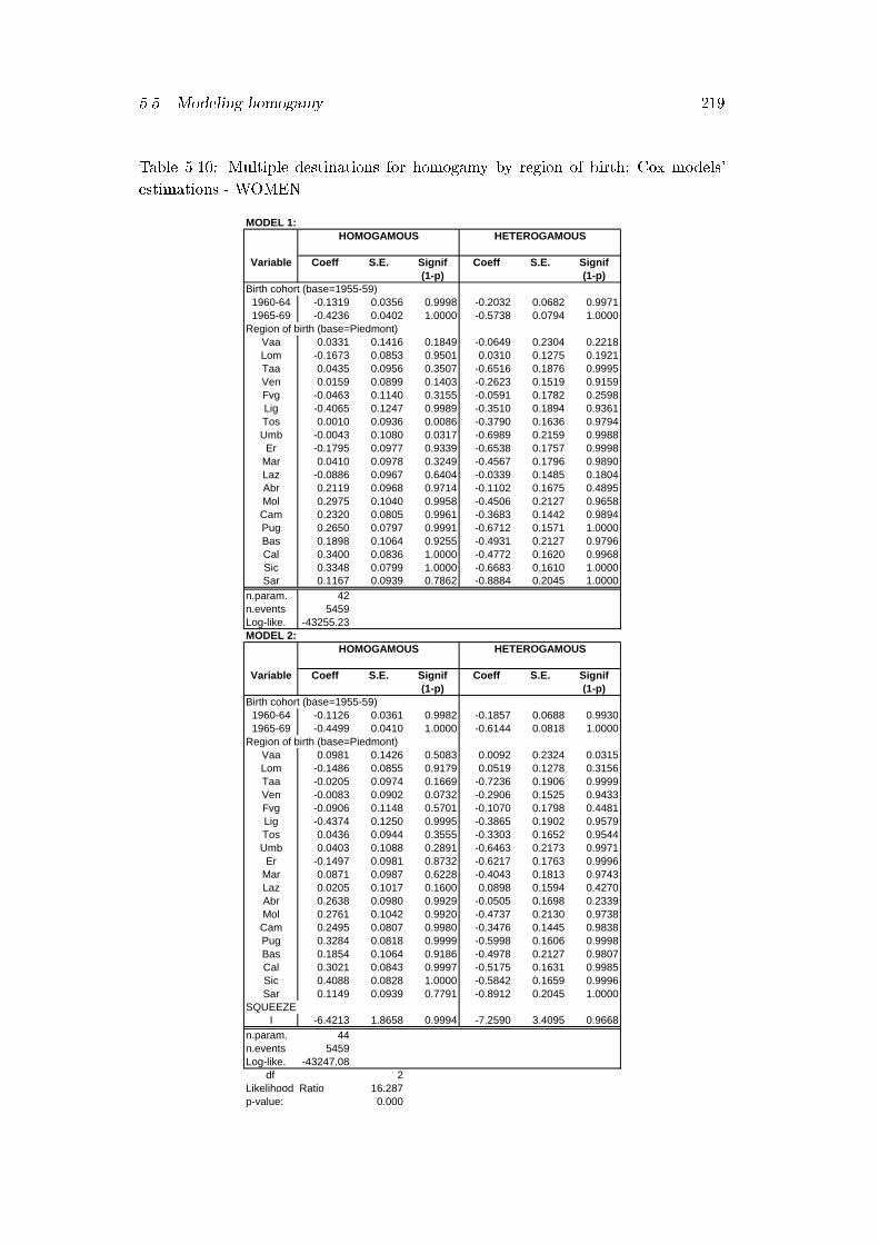
5.5. Modeling homogamy 219
Table 5.10: Multiple destinations for homogamy by region of birth; Cox models'
estimations - WOMEN
MODEL 1:
Variable Coeff S.E. Signif Coeff S.E. Signif(1-p) (1-p)
Birth cohort (base=1955-59)1960-64 -0.1319 0.0356 0.9998 -0.2032 0.0682 0.99711965-69 -0.4236 0.0402 1.0000 -0.5738 0.0794 1.0000
Region of birth (base=Piedmont)Vaa 0.0331 0.1416 0.1849 -0.0649 0.2304 0.2218Lom -0.1673 0.0853 0.9501 0.0310 0.1275 0.1921Taa 0.0435 0.0956 0.3507 -0.6516 0.1876 0.9995Ven 0.0159 0.0899 0.1403 -0.2623 0.1519 0.9159Fvg -0.0463 0.1140 0.3155 -0.0591 0.1782 0.2598Lig -0.4065 0.1247 0.9989 -0.3510 0.1894 0.9361Tos 0.0010 0.0936 0.0086 -0.3790 0.1636 0.9794Umb -0.0043 0.1080 0.0317 -0.6989 0.2159 0.9988
Er -0.1795 0.0977 0.9339 -0.6538 0.1757 0.9998Mar 0.0410 0.0978 0.3249 -0.4567 0.1796 0.9890Laz -0.0886 0.0967 0.6404 -0.0339 0.1485 0.1804Abr 0.2119 0.0968 0.9714 -0.1102 0.1675 0.4895Mol 0.2975 0.1040 0.9958 -0.4506 0.2127 0.9658Cam 0.2320 0.0805 0.9961 -0.3683 0.1442 0.9894Pug 0.2650 0.0797 0.9991 -0.6712 0.1571 1.0000Bas 0.1898 0.1064 0.9255 -0.4931 0.2127 0.9796Cal 0.3400 0.0836 1.0000 -0.4772 0.1620 0.9968Sic 0.3348 0.0799 1.0000 -0.6683 0.1610 1.0000Sar 0.1167 0.0939 0.7862 -0.8884 0.2045 1.0000
n.param. 42n.events 5459Log-like. -43255.23MODEL 2:
Variable Coeff S.E. Signif Coeff S.E. Signif(1-p) (1-p)
Birth cohort (base=1955-59)1960-64 -0.1126 0.0361 0.9982 -0.1857 0.0688 0.99301965-69 -0.4499 0.0410 1.0000 -0.6144 0.0818 1.0000
Region of birth (base=Piedmont)Vaa 0.0981 0.1426 0.5083 0.0092 0.2324 0.0315Lom -0.1486 0.0855 0.9179 0.0519 0.1278 0.3156Taa -0.0205 0.0974 0.1669 -0.7236 0.1906 0.9999Ven -0.0083 0.0902 0.0732 -0.2906 0.1525 0.9433Fvg -0.0906 0.1148 0.5701 -0.1070 0.1798 0.4481Lig -0.4374 0.1250 0.9995 -0.3865 0.1902 0.9579Tos 0.0436 0.0944 0.3555 -0.3303 0.1652 0.9544Umb 0.0403 0.1088 0.2891 -0.6463 0.2173 0.9971
Er -0.1497 0.0981 0.8732 -0.6217 0.1763 0.9996Mar 0.0871 0.0987 0.6228 -0.4043 0.1813 0.9743Laz 0.0205 0.1017 0.1600 0.0898 0.1594 0.4270Abr 0.2638 0.0980 0.9929 -0.0505 0.1698 0.2339Mol 0.2761 0.1042 0.9920 -0.4737 0.2130 0.9738Cam 0.2495 0.0807 0.9980 -0.3476 0.1445 0.9838Pug 0.3284 0.0818 0.9999 -0.5998 0.1606 0.9998Bas 0.1854 0.1064 0.9186 -0.4978 0.2127 0.9807Cal 0.3021 0.0843 0.9997 -0.5175 0.1631 0.9985Sic 0.4088 0.0828 1.0000 -0.5842 0.1659 0.9996Sar 0.1149 0.0939 0.7791 -0.8912 0.2045 1.0000
SQUEEZEI -6.4213 1.8658 0.9994 -7.2590 3.4095 0.9668
n.param. 44n.events 5459Log-like. -43247.08
df 2Likelihood Ratio 16.287p-value: 0.000
HOMOGAMOUS HETEROGAMOUS
HOMOGAMOUS HETEROGAMOUS
220 Chapter 5. Trends in homogamy
it is worth noting that overall, being born in one of the northern regions reduces,
the competing risk of marrying a woman of the same place of origin in comparison
to that of out-marrying, while being born in the South increases the chances to
marry homogamously. It is also interesting to see that two big and very attractive
(especially as concerns the labour market) regions, such as Lombardy and Lazio
show to have a slower than Piedmont transition to same-region marriages and a
shorter waiting time for di�erent-region marriage. This is to say that men born
in one of these two regions experience a rise in their chances to marry a woman
born somewhere else, and a decline in the chances to marry one of the same region.
This also con�rms the hypothesis concerning the geographical isolation of some
southern regions. Introducing the e�ect of the squeeze, S for men, determines an
increase in the transition rate of both destinations, but heterogamous marriages
are fairly higher than homogamous marriages (table 5.9 Model 2). If men have an
advantage on the marriage market, then their chances to marry rise quickly, above
all heterogamously. This could be attributed to their higher mobility which enhances
their marriage market conditions, improving their chances to out-marrying.
As concerns women, each successive cohort shows to have a rate which indicates
the slow down of the transition to �rst marriages in both directions (tables 5.10,
Model 1): cohorts younger than the 1955-59 one, wait longer before marrying, espe-
cially if the partner was born in a di�erent region (heterogamous). Women con�rm
also the tendency to marry a man from the same place of origin in the South more
than in the North: being born in the South increases the transition to marriages
with same-region partners, and decreases the competing risk to marry a man coming
from a di�erent region. This is equivalent to say that southern women accelerate
their rate of marriage with a mate born in the same region, while heterogamous mar-
riages are postponed, especially in the islands (when compared to Piedmont, Sicily
has a coe�cient for heterogamous marriages equal -0.6683 and Sardinia equals to -
0.8884). Moreover, homogamous marriages are postponed by women only when born
in Lombardy, Lazio, Emilia Romagna, Liguria, Friuli Venezia Giulia and Umbria:
these represent attractive labour markets on one side and small regions on the other
side. It is worth noting that women born both in Lazio and in Lombardy further
reduce their transition to homogamous marriages. The disadvantage in the marriage
5.5. Modeling homogamy 221
market induces a further postponement of �rst marriages in both directions: either
the hazard of homogamous (-6.4213) and that of heterogamous marriages (-7.2590)
address a slow down of marriage occurrence, a bit larger for marriages to men born
in a di�erent region (table 5.10 Model 2).
In sum, the place of origin is loosing part of its relevant role as marriage market
especially for men, which experience a comparatively higher decline in the transition
to endogamous marriages than to exogamous. A major explanation for men could be
attributed to their higher mobility (especially if born in some central and northern
regions) which eases the meeting with women born in di�erent regions enlarging the
pool of availability. Women show to have a di�erent dynamics: the marriage market
in which they play a major role is represented by their region of birth: for women
heterogamous marriages decline more than endogamous ones. Their lower mobility,
narrowing their marriage market to that of their region of birth, also worsen their
chances to out-marriage. The traditional model based on a stronger homogamy in
the southern regions still holds. Some regions have also a peculiar attractive role
which eases out-marriages, some other su�er for their isolation and the consequent
di�culties.
5.5.3 Homogamy by education
Education is probably one of the most important trait for its potential capacity
in attributing partners' future traits. Our attention is here particularly oriented
towards the analysis of di�erences among cohorts and among regions: we are inter-
ested in studying trends in male and female homogamy by education and regional
di�erences. In fact, a measure of the characteristics of the marriage market express-
ing the imbalance between the sexes in terms of achieved education is not available:
the measures of the squeeze which we built are not education-speci�c and they could
result not adequate to our purposes. However, one of our attempt is to see whether
the imbalance in the marriage market, as expressed up to now could be meaningful
to our educational homogamy analysis.
For low educated women (2628) increase the percentage of lateral marriages, for
high educated women (2821) increases the percentage of downward marriages (table
5.11); men with low education (2331) have a slight decrease in lateral marriages and
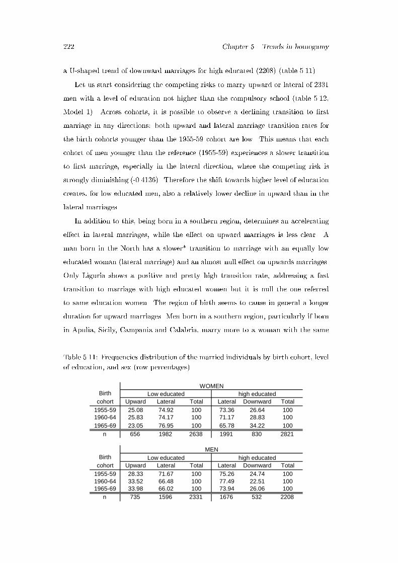
222 Chapter 5. Trends in homogamy
a U-shaped trend of downward marriages for high educated (2208) (table 5.11).
Let us start considering the competing risks to marry upward or lateral of 2331
men with a level of education not higher than the compulsory school (table 5.12,
Model 1). Across cohorts, it is possible to observe a declining transition to �rst
marriage in any directions: both upward and lateral marriage transition rates for
the birth cohorts younger than the 1955-59 cohort are low. This means that each
cohort of men younger than the reference (1955-59) experiences a slower transition
to �rst marriage, especially in the lateral direction, where the competing risk is
strongly diminishing (-0.4136). Therefore the shift towards higher level of education
creates, for low educated men, also a relatively lower decline in upward than in the
lateral marriages.
In addition to this, being born in a southern region, determines an accelerating
e�ect in lateral marriages, while the e�ect on upward marriages is less clear. A
man born in the North has a slower* transition to marriage with an equally low
educated woman (lateral marriage) and an almost null e�ect on upwards marriages.
Only Liguria shows a positive and pretty high transition rate, addressing a fast
transition to marriage with high educated women but it is null the one referred
to same education women. The region of birth seems to cause in general a longer
duration for upward marriages. Men born in a southern region, particularly if born
in Apulia, Sicily, Campania and Calabria, marry more to a woman with the same
Table 5.11: Frequencies distribution of the married individuals by birth cohort, level
of education, and sex (row percentages)
Birthcohort Upward Lateral Total Lateral Downward Total
1955-59 25.08 74.92 100 73.36 26.64 1001960-64 25.83 74.17 100 71.17 28.83 1001965-69 23.05 76.95 100 65.78 34.22 100
n 656 1982 2638 1991 830 2821
Birthcohort Upward Lateral Total Lateral Downward Total
1955-59 28.33 71.67 100 75.26 24.74 1001960-64 33.52 66.48 100 77.49 22.51 1001965-69 33.98 66.02 100 73.94 26.06 100
n 735 1596 2331 1676 532 2208
WOMEN
high educatedLow educated
Low educated high educated
MEN
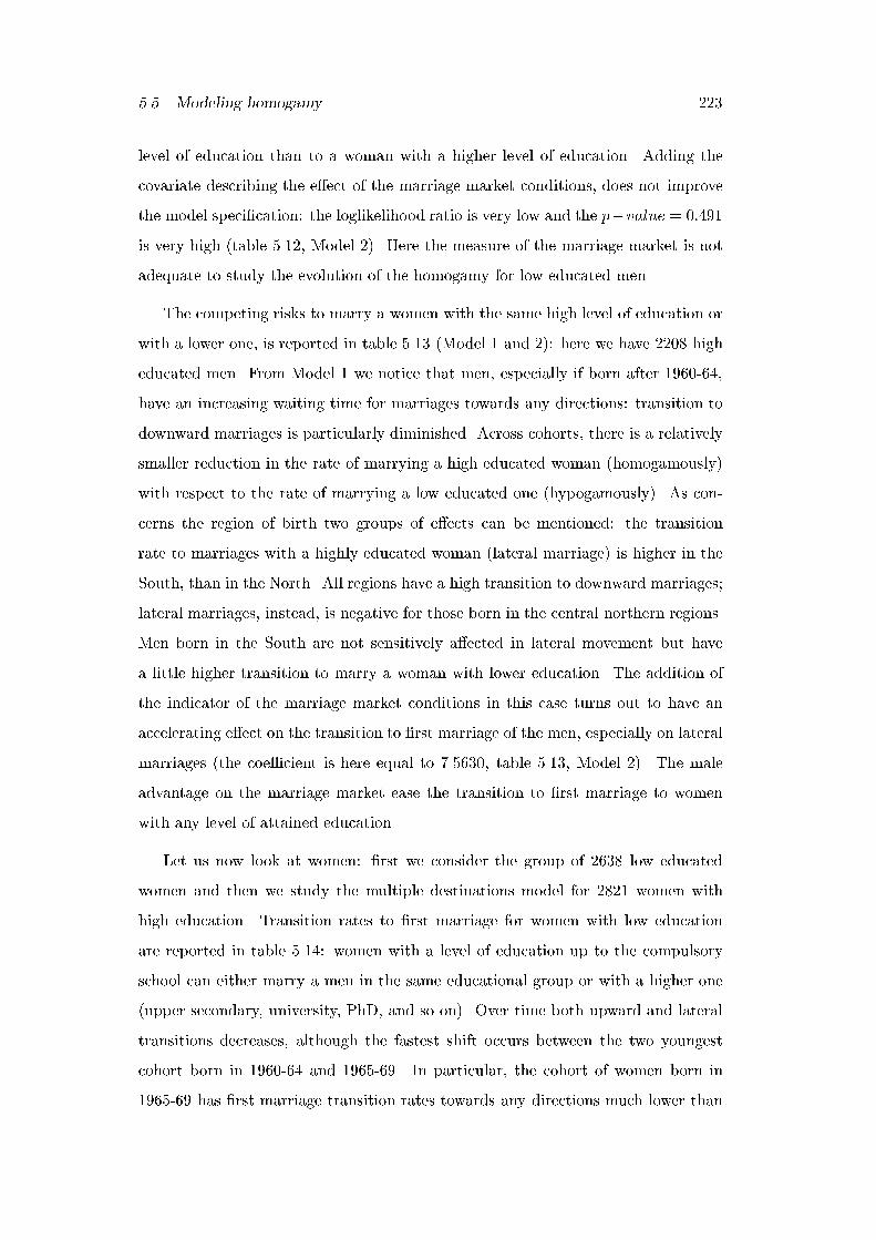
5.5. Modeling homogamy 223
level of education than to a woman with a higher level of education. Adding the
covariate describing the e�ect of the marriage market conditions, does not improve
the model speci�cation: the loglikelihood ratio is very low and the p�value = 0:491
is very high (table 5.12, Model 2). Here the measure of the marriage market is not
adequate to study the evolution of the homogamy for low educated men.
The competing risks to marry a women with the same high level of education or
with a lower one, is reported in table 5.13 (Model 1 and 2): here we have 2208 high
educated men. From Model 1 we notice that men, especially if born after 1960-64,
have an increasing waiting time for marriages towards any directions: transition to
downward marriages is particularly diminished. Across cohorts, there is a relatively
smaller reduction in the rate of marrying a high educated woman (homogamously)
with respect to the rate of marrying a low educated one (hypogamously). As con-
cerns the region of birth two groups of e�ects can be mentioned: the transition
rate to marriages with a highly educated woman (lateral marriage) is higher in the
South, than in the North. All regions have a high transition to downward marriages;
lateral marriages, instead, is negative for those born in the central northern regions.
Men born in the South are not sensitively a�ected in lateral movement but have
a little higher transition to marry a woman with lower education. The addition of
the indicator of the marriage market conditions in this case turns out to have an
accelerating e�ect on the transition to �rst marriage of the men, especially on lateral
marriages (the coe�cient is here equal to 7.5630, table 5.13, Model 2). The male
advantage on the marriage market ease the transition to �rst marriage to women
with any level of attained education.
Let us now look at women: �rst we consider the group of 2638 low educated
women and then we study the multiple destinations model for 2821 women with
high education. Transition rates to �rst marriage for women with low education
are reported in table 5.14: women with a level of education up to the compulsory
school can either marry a men in the same educational group or with a higher one
(upper secondary, university, PhD, and so on). Over time both upward and lateral
transitions decreases, although the fastest shift occurs between the two youngest
cohort born in 1960-64 and 1965-69. In particular, the cohort of women born in
1965-69 has �rst marriage transition rates towards any directions much lower than
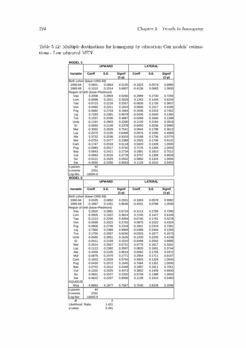
224 Chapter 5. Trends in homogamy
Table 5.12: Multiple destinations for homogamy by education; Cox models' estima-
tions - Low educated MEN
MODEL 1:
Variable Coeff S.E. Signif Coeff S.E. Signif(1-p) (1-p)
Birth cohort (base=1955-59)1960-64 0.0601 0.0864 0.5135 -0.1823 0.0574 0.99851965-69 -0.1010 0.1014 0.6807 -0.4136 0.0683 1.0000
Region of birth (base=Piedmont)Vaa 0.2008 0.2804 0.5260 -0.2989 0.2730 0.7265Lom -0.0988 0.1921 0.3929 0.1263 0.1426 0.6244Taa -0.0723 0.2216 0.2557 -0.0826 0.1735 0.3657Ven -0.0460 0.2011 0.1810 0.0836 0.1517 0.4185Fvg -0.0682 0.2743 0.1964 -0.2636 0.2315 0.7452Lig 0.7293 0.2381 0.9978 -0.0426 0.2440 0.1385Tos 0.1337 0.2036 0.4887 -0.0269 0.1660 0.1288Umb -0.1191 0.2803 0.3290 -0.1120 0.2184 0.3918Er -0.0650 0.2149 0.2378 -0.6455 0.2036 0.9985
Mar -0.3062 0.2639 0.7541 0.0844 0.1798 0.3613Laz -0.2075 0.2235 0.6468 0.0975 0.1595 0.4589Abr 0.3732 0.2036 0.9333 0.0168 0.1736 0.0770Mol -0.0753 0.2477 0.2388 0.2925 0.1708 0.9132Cam -0.1747 0.2024 0.6118 0.5920 0.1328 1.0000Pug -0.0983 0.2017 0.3740 0.7176 0.1306 1.0000Bas 0.0843 0.2411 0.2734 0.1881 0.1810 0.7012Cal -0.0993 0.2016 0.3778 0.3757 0.1399 0.9928Sic -0.0121 0.1929 0.0502 0.5850 0.1324 1.0000Sar -0.4550 0.2256 0.9563 0.1129 0.1510 0.5453
n.param. 42n.events 2331Log-like. -16694.6MODEL 2:
Variable Coeff S.E. Signif Coeff S.E. Signif(1-p) (1-p)
Birth cohort (base=1955-59)1960-64 0.0335 0.0892 0.2931 -0.1803 0.0578 0.99821965-69 -0.1867 0.1251 0.8646 -0.4031 0.0788 1.0000
Region of birth (base=Piedmont)Vaa 0.2820 0.2881 0.6724 -0.3113 0.2769 0.7390Lom -0.0905 0.1922 0.3624 0.1245 0.1427 0.6169Taa -0.1213 0.2256 0.4094 -0.0745 0.1761 0.3278Ven -0.0699 0.2022 0.2703 0.0870 0.1522 0.4324Fvg -0.0809 0.2745 0.2318 -0.2601 0.2319 0.7381Lig 0.7066 0.2389 0.9969 -0.0388 0.2444 0.1260Tos 0.1750 0.2067 0.6030 -0.0333 0.1677 0.1573Umb -0.0585 0.2851 0.1626 -0.1200 0.2205 0.4138Er -0.0411 0.2159 0.1510 -0.6498 0.2042 0.9985
Mar -0.2614 0.2667 0.6731 0.0775 0.1817 0.3301Laz -0.1113 0.2382 0.3597 0.0825 0.1691 0.3744Abr 0.4359 0.2105 0.9616 0.0082 0.1765 0.0372Mol -0.0879 0.2479 0.2771 0.2954 0.1711 0.9157Cam -0.1602 0.2029 0.5704 0.5903 0.1329 1.0000Pug -0.0430 0.2072 0.1645 0.7084 0.1351 1.0000Bas 0.0752 0.2412 0.2448 0.1897 0.1811 0.7051Cal -0.1202 0.2025 0.4473 0.3802 0.1409 0.9930Sic 0.0601 0.2027 0.2332 0.5739 0.1388 1.0000Sar -0.4622 0.2257 0.9595 0.1139 0.1510 0.5493
SQUEEZEIfreq -4.8863 4.1877 0.7567 0.7540 2.8328 0.2099
n.param. 44n.events 2331Log-like. -16693.9
df 2Likelihood Ratio 1.421p-value: 0.491
UPWARD LATERAL
UPWARD LATERAL

5.5. Modeling homogamy 225
Table 5.13: Multiple destinations for homogamy by education; Cox models' estima-
tions - High educated MEN
MODEL 1:
Variable Coeff S.E. Signif Coeff S.E. Signif(1-p) (1-p)
Birth cohort (base=1955-59)1960-64 -0.0301 0.0546 0.4183 -0.2150 0.0974 0.97281965-69 -0.3418 0.0766 1.0000 -0.5091 0.1282 0.9999
Region of birth (base=Piedmont)Vaa -0.6470 0.2748 0.9814 -0.2545 0.4847 0.4005Lom -0.1659 0.1298 0.7988 0.0977 0.2443 0.3109Taa -0.2008 0.1585 0.7950 0.4324 0.2627 0.9002Ven -0.3199 0.1436 0.9741 0.3173 0.2467 0.8016Fvg -0.1457 0.1672 0.6165 0.3489 0.2866 0.7766Lig -0.2120 0.1673 0.7951 -0.4274 0.3669 0.7560Tos 0.0219 0.1399 0.1244 0.3966 0.2529 0.8832Umb -0.0417 0.1538 0.2139 0.0826 0.2953 0.2201Er -0.3373 0.1497 0.9757 -0.0487 0.2793 0.1384
Mar -0.1751 0.1484 0.7619 0.1978 0.2675 0.5405Laz 0.0347 0.1344 0.2038 -0.1655 0.2828 0.4417Abr 0.1831 0.1446 0.7947 0.1068 0.2907 0.2865Mol -0.1776 0.1641 0.7209 -0.2097 0.3339 0.4699Cam 0.0191 0.1261 0.1204 0.2857 0.2372 0.7717Pug -0.0451 0.1269 0.2776 0.1494 0.2427 0.4618Bas -0.1156 0.1612 0.5266 -0.1105 0.3255 0.2658Cal -0.0423 0.1347 0.2468 0.2908 0.2481 0.7589Sic 0.0759 0.1277 0.4475 0.2601 0.2441 0.7134Sar -0.0792 0.1672 0.3644 0.5034 0.2760 0.9318
n.param. 42n.events 2208Log-like. -15846.3MODEL 2:
Variable Coeff S.E. Signif Coeff S.E. Signif(1-p) (1-p)
Birth cohort (base=1955-59)1960-64 0.0359 0.0612 0.4429 -0.1988 0.1011 0.95081965-69 -0.1813 0.1014 0.9261 -0.4546 0.1569 0.9962
Region of birth (base=Piedmont)Vaa -0.7698 0.2802 0.9940 -0.3002 0.4910 0.4591Lom -0.1862 0.1300 0.8478 0.0886 0.2448 0.2826Taa -0.1253 0.1615 0.5622 0.4653 0.2683 0.9171Ven -0.2915 0.1441 0.9570 0.3283 0.2473 0.8156Fvg -0.1374 0.1672 0.5886 0.3584 0.2870 0.7883Lig -0.1775 0.1679 0.7095 -0.4117 0.3678 0.7370Tos -0.0510 0.1432 0.2783 0.3689 0.2571 0.8487Umb -0.1378 0.1589 0.6142 0.0512 0.3000 0.1354Er -0.3728 0.1505 0.9868 -0.0655 0.2807 0.1844
Mar -0.2447 0.1512 0.8944 0.1698 0.2715 0.4684Laz -0.1236 0.1494 0.5918 -0.2289 0.3018 0.5518Abr 0.0777 0.1510 0.3931 0.0698 0.2972 0.1858Mol -0.1724 0.1641 0.7065 -0.2013 0.3342 0.4530Cam -0.0106 0.1267 0.0665 0.2763 0.2377 0.7549Pug -0.1231 0.1310 0.6527 0.1154 0.2492 0.3566Bas -0.1062 0.1612 0.4900 -0.1046 0.3257 0.2520Cal -0.0183 0.1350 0.1075 0.3078 0.2496 0.7824Sic -0.0403 0.1363 0.2323 0.2145 0.2555 0.5987Sar -0.0690 0.1672 0.3202 0.5070 0.2761 0.9337
SQUEEZEIfreq 7.5630 3.1227 0.9846 3.0656 5.0941 0.4527
n.param. 44n.events 2208Log-like. -15843.2
df 2Likelihood Ratio 6.291p-value: 0.043
LATERAL DOWNWARD
LATERAL DOWNWARD

226 Chapter 5. Trends in homogamy
the reference cohort (women born in 1955-59). While for the birth cohort 1960-
64 the reduction in the rate a�ects almost equally both destinations and it is not
particularly relevant, for the women born in 1965-69 especially upward marriages
are postponed. Compared to those born in 1955-59, the transition rate for the 1965-
69 women is -0.5463 for marrying a higher educated partner and it is -0.4507 for a
same-schooling mate (table 5.14). Therefore, low educated women, experience over
time a comparatively higher decline in upward marriages (to more educated men)
than in lateral marriages (to a man with same education).
Being born in one of the southern regions seems to determine a slightly higher
transition rate to marry an equally low educated men (lateral) and lower rate of
marriage to a highly educated men. Low educated women born in the northern-
central regions have in general low transition rates both to marry a men with the
same level of education (lateral) or a more educated one (upward), but the former
rate is always lower than the latter one.
Including the measure of the marriage squeeze determines a small improvement
of the log-likelihood but it does not have a clear e�ect. Lateral movements are
strongly postponed in the case of a female disadvantage on the marriage market
(the coe�cient is equal to -11.5104 and it is signi�cant), while upward marriage
seems to be enhanced by the squeeze's increase. Caution should be used in this
case, given that the coe�cient of the squeeze to marry up is not signi�cant and that
we are talking about an amount of only 656 women (those marrying up). In sum,
younger cohort of low educated women reduce their transition to �rst marriage, in
particular upwardly; lateral movements are higher in the southern regions while in
the North they are comparatively lower than the upward ones. The male advantage
on the marriage market strongly reduced the chances to marry a man with the same
low education, while it is not clear the e�ect on upward movements.
Let us now look at the women with a high education (including more than 8 years
schooling): here we have 2821 women, 1991 of which married a man with longer than
8 years schooling as well, and 830 married a man who studied shorter (table 5.15).
In comparison to the older birth cohort, younger women have a longer duration of
the waiting time for the �rst marriage. Moreover, in each younger cohort compared
to the 1955-59 one, the competing risk of marrying a high educated man (lateral
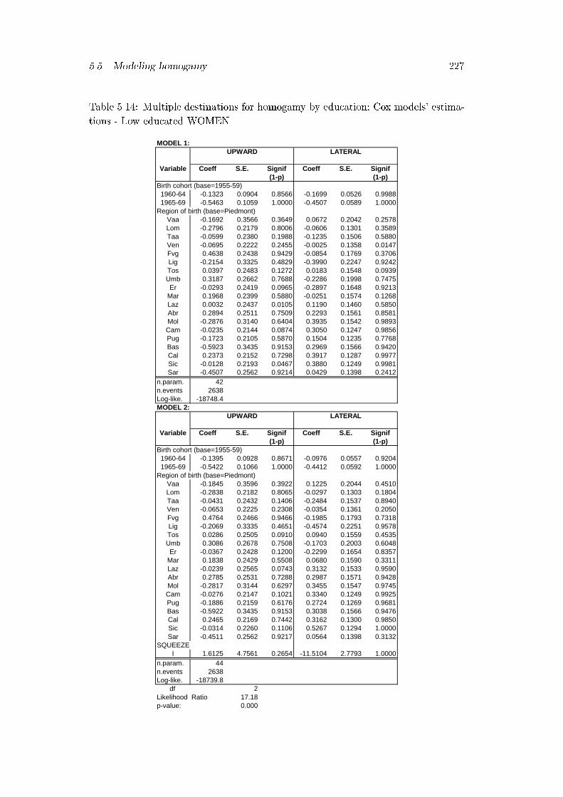
5.5. Modeling homogamy 227
Table 5.14: Multiple destinations for homogamy by education; Cox models' estima-
tions - Low educated WOMEN
MODEL 1:
Variable Coeff S.E. Signif Coeff S.E. Signif(1-p) (1-p)
Birth cohort (base=1955-59)1960-64 -0.1323 0.0904 0.8566 -0.1699 0.0526 0.99881965-69 -0.5463 0.1059 1.0000 -0.4507 0.0589 1.0000
Region of birth (base=Piedmont)Vaa -0.1692 0.3566 0.3649 0.0672 0.2042 0.2578Lom -0.2796 0.2179 0.8006 -0.0606 0.1301 0.3589Taa -0.0599 0.2380 0.1988 -0.1235 0.1506 0.5880Ven -0.0695 0.2222 0.2455 -0.0025 0.1358 0.0147Fvg 0.4638 0.2438 0.9429 -0.0854 0.1769 0.3706Lig -0.2154 0.3325 0.4829 -0.3990 0.2247 0.9242Tos 0.0397 0.2483 0.1272 0.0183 0.1548 0.0939Umb 0.3187 0.2662 0.7688 -0.2286 0.1998 0.7475Er -0.0293 0.2419 0.0965 -0.2897 0.1648 0.9213
Mar 0.1968 0.2399 0.5880 -0.0251 0.1574 0.1268Laz 0.0032 0.2437 0.0105 0.1190 0.1460 0.5850Abr 0.2894 0.2511 0.7509 0.2293 0.1561 0.8581Mol -0.2876 0.3140 0.6404 0.3935 0.1542 0.9893Cam -0.0235 0.2144 0.0874 0.3050 0.1247 0.9856Pug -0.1723 0.2105 0.5870 0.1504 0.1235 0.7768Bas -0.5923 0.3435 0.9153 0.2969 0.1566 0.9420Cal 0.2373 0.2152 0.7298 0.3917 0.1287 0.9977Sic -0.0128 0.2193 0.0467 0.3880 0.1249 0.9981Sar -0.4507 0.2562 0.9214 0.0429 0.1398 0.2412
n.param. 42n.events 2638Log-like. -18748.4MODEL 2:
Variable Coeff S.E. Signif Coeff S.E. Signif(1-p) (1-p)
Birth cohort (base=1955-59)1960-64 -0.1395 0.0928 0.8671 -0.0976 0.0557 0.92041965-69 -0.5422 0.1066 1.0000 -0.4412 0.0592 1.0000
Region of birth (base=Piedmont)Vaa -0.1845 0.3596 0.3922 0.1225 0.2044 0.4510Lom -0.2838 0.2182 0.8065 -0.0297 0.1303 0.1804Taa -0.0431 0.2432 0.1406 -0.2484 0.1537 0.8940Ven -0.0653 0.2225 0.2308 -0.0354 0.1361 0.2050Fvg 0.4764 0.2466 0.9466 -0.1985 0.1793 0.7318Lig -0.2069 0.3335 0.4651 -0.4574 0.2251 0.9578Tos 0.0286 0.2505 0.0910 0.0940 0.1559 0.4535Umb 0.3086 0.2678 0.7508 -0.1703 0.2003 0.6048Er -0.0367 0.2428 0.1200 -0.2299 0.1654 0.8357
Mar 0.1838 0.2429 0.5508 0.0680 0.1590 0.3311Laz -0.0239 0.2565 0.0743 0.3132 0.1533 0.9590Abr 0.2785 0.2531 0.7288 0.2987 0.1571 0.9428Mol -0.2817 0.3144 0.6297 0.3455 0.1547 0.9745Cam -0.0276 0.2147 0.1021 0.3340 0.1249 0.9925Pug -0.1886 0.2159 0.6176 0.2724 0.1269 0.9681Bas -0.5922 0.3435 0.9153 0.3038 0.1566 0.9476Cal 0.2465 0.2169 0.7442 0.3162 0.1300 0.9850Sic -0.0314 0.2260 0.1106 0.5267 0.1294 1.0000Sar -0.4511 0.2562 0.9217 0.0564 0.1398 0.3132
SQUEEZEI 1.6125 4.7561 0.2654 -11.5104 2.7793 1.0000
n.param. 44n.events 2638Log-like. -18739.8
df 2Likelihood Ratio 17.18p-value: 0.000
UPWARD LATERAL
UPWARD LATERAL
228 Chapter 5. Trends in homogamy
marriage) is much lower than that of marrying a lower educated man (downward
marriage). So high educated women have a longer waiting time for marrying a man
with the same educational attainment: we do not not whether this will bring about
postponing or giving up to marriages of a certain `quality' (a given destination).
The growth in the female educational attainment can increase the di�culties for
women in �nding a partner with the same (high) level of education among the pool
of eligibles. Most of the regions of birth have a lower rate for downward marriages
than for lateral. So women have a lower risk to marry down than educationally
homogamous. Moreover central regions represent a group with very low rate to
downward marriage. Besides that, some of the southern regions (namely Campania,
Apulia, Abruzzo and Molise) have a positive e�ect to marry laterally and high and
negative to marry downwardly. It is worth noting that highly educated women born
in these regions, have a very high reduction in the risk of marrying downwardly
(the coe�cient being signi�cant and equal to -0.6228 and -0.6297 for Campania and
Apulia) and a small, although not signi�cant, increase in the risk of marrying lateral
than in Piedmont. Also other regions (Umbria, Liguria Marches, Lazio) experience
a strong postponement of downward marriage, but the same reduction occurs also
for lateral marriages. The introduction of the time-varying covariate squeeze (S)
improves the log-likelihood and addresses the existence of a disadvantage in marrying
a lower educated mate (lateral). The chances of a woman to marry a men of the
same level of education do not seem to be a�ected by the squeeze against women
(the coe�cient is virtually null). Conversely, it is clear that the male advantage in
the marriage market further postpones downward marriages for women with high
education.
5.6 Summary and discussion
In this chapter we presented an analysis of marriage in Italy, under a di�erent
perspective: we looked at characteristics of the partners at their �rst marriage and
studied the trends in homogamy by age, place of origin and education of the spouses.
Coherently to what accomplished in preceding chapters, the approach we pursed is
that of an event history analysis.
Overall, the prevailing patterns of marriage are the more traditional ones: the

5.6. Summary and discussion 229
Table 5.15: Multiple destinations for homogamy by education; Cox models' estima-
tions - High educated WOMEN
MODEL 1:
Variable Coeff S.E. Signif Coeff S.E. Signif(1-p) (1-p)
Birth cohort (base=1955-59)1960-64 -0.1566 0.0521 0.9974 -0.0742 0.0840 0.62301965-69 -0.5059 0.0610 1.0000 -0.2512 0.0909 0.9943
Region of birth (base=Piedmont)Vaa -0.4785 0.2436 0.9505 0.4312 0.2341 0.9345Lom -0.1515 0.1130 0.8200 -0.1684 0.1597 0.7082Taa -0.2111 0.1402 0.8680 -0.2609 0.2003 0.8073Ven -0.2194 0.1314 0.9051 -0.2196 0.1833 0.7691Fvg -0.2254 0.1588 0.8443 -0.3790 0.2421 0.8825Lig -0.4288 0.1547 0.9944 -0.3632 0.2181 0.9041Tos -0.1784 0.1261 0.8428 -0.1837 0.1786 0.6964Umb -0.0577 0.1384 0.3231 -0.7524 0.2563 0.9967Er -0.4560 0.1363 0.9992 -0.2364 0.1830 0.8036
Mar -0.0785 0.1324 0.4468 -0.6456 0.2270 0.9955Laz -0.1618 0.1282 0.7931 -0.4090 0.1966 0.9625Abr 0.0784 0.1306 0.4516 -0.1001 0.1934 0.3953Mol 0.0227 0.1518 0.1186 -0.2520 0.2380 0.7104Cam 0.0658 0.1098 0.4510 -0.6228 0.1878 0.9991Pug 0.1442 0.1117 0.8033 -0.6297 0.1950 0.9988Bas -0.0887 0.1565 0.4291 -0.2052 0.2303 0.6272Cal -0.0645 0.1223 0.4021 -0.2099 0.1820 0.7512Sic -0.0103 0.1130 0.0727 -0.3239 0.1739 0.9374Sar -0.4658 0.1577 0.9969 0.0519 0.1893 0.2160
n.param. 42n.events 2821Log-like. -20689.1MODEL 2:
Variable Coeff S.E. Signif Coeff S.E. Signif(1-p) (1-p)
Birth cohort (base=1955-59)1960-64 -0.1565 0.0521 0.9973 -0.0309 0.0853 0.28281965-69 -0.5051 0.0680 1.0000 -0.3358 0.0939 0.9996
Region of birth (base=Piedmont)Vaa -0.4796 0.2473 0.9475 0.6092 0.2373 0.9897Lom -0.1518 0.1135 0.8188 -0.1205 0.1602 0.5480Taa -0.2105 0.1424 0.8605 -0.4001 0.2037 0.9505Ven -0.2190 0.1320 0.9030 -0.2818 0.1841 0.8741Fvg -0.2251 0.1592 0.8428 -0.4685 0.2435 0.9456Lig -0.4285 0.1553 0.9942 -0.4319 0.2189 0.9516Tos -0.1789 0.1278 0.8384 -0.0819 0.1806 0.3496Umb -0.0584 0.1409 0.3213 -0.6388 0.2581 0.9867Er -0.4564 0.1368 0.9991 -0.1651 0.1839 0.6305
Mar -0.0790 0.1340 0.4447 -0.5392 0.2288 0.9816Laz -0.1631 0.1378 0.7635 -0.1493 0.2085 0.5260Abr 0.0776 0.1339 0.4380 0.0379 0.1968 0.1527Mol 0.0228 0.1519 0.1193 -0.2970 0.2384 0.7873Cam 0.0656 0.1102 0.4482 -0.5778 0.1883 0.9978Pug 0.1435 0.1150 0.7880 -0.4848 0.1988 0.9852Bas -0.0886 0.1566 0.4286 -0.2195 0.2303 0.6594Cal -0.0641 0.1231 0.3978 -0.2983 0.1836 0.8958Sic -0.0112 0.1180 0.0754 -0.1465 0.1806 0.5828Sar -0.4657 0.1577 0.9968 0.0401 0.1894 0.1675
SQUEEZES 0.0373 1.4696 0.0203 -7.6235 2.0506 0.9998
n.param. 44n.events 2821Log-like. -20682.3
df 2Likelihood Ratio 13.65p-value: 0.001
LATERAL DOWNWARD
LATERAL DOWNWARD
230 Chapter 5. Trends in homogamy
prevailing propensity is towards a marriage where the husband is older than the wife,
where they both are born in the same region of birth and where they have attained,
broadly speaking, the same level of education. Despite of the persistency of the
traditional patterns of homogamy, some new features in the process of assortative
mating are rising in Italy. In particular, the modernisation theory provides us with
some useful tools of interpretation of the recent developments in homogamy patterns.
For instance, more age-balanced couples are the natural outcome of a reduced gender
division and a higher equalisation of the roles in the couple. As concerns Italy,
men experience a relative decrease of the transition rate for the traditional age-gap
between partners, and a slight increase of the atypical matches characterised by
higher age of the woman. Conversely, for women the traditional pattern is the only
one, although the youngest cohorts show a slowing down of the process which could
determine next years a change in the sign, thereby an emerging of more age-balanced
union. Men and women born in the North are more oriented to this new typology
of age-balance between couple, re ecting also a higher gender equalisation, while
southern men hold a higher attachment to large age di�erences between partners.
The diminishing role of the place of origin in assortative mating is found as
expected. There is a stronger decline of marriages between partners coming from the
same regions, especially for men whose mobility enlarges their pool and enhances
their chances to marry heterogamously. Women on the other hand, have bigger
di�culties in out-marrying, especially if they are born in the South, where the
general level of mobility is small in comparison to the central and northern regions.
Furthermore it emerges the role of some regions at the borders of the country with
decreasing heterogamy, as well as that of more attractive regions characterised also
by greater heterogamous marriages.
It is puzzling to understand whether in the future the e�ects of the globalisation,
of the easiness of the communication and of the speedy of mobility will increasingly
enlarge the opportunities to out-marry, involving both sexes: it could be expected
a growing `loss of meaning' of the region of birth as determinant of the marriage
opportunities.
Homogamy by level of education is a bit less clear. For men, a slight growth
in the propensity to marry to women with education higher than theirs can be

5.6. Summary and discussion 231
noticed: this emerges from the fact that men with high education reduce less the
rate of homogamous marriages, while men with low education reduce less the rate
of upward rate. This is the outcome of a grown attractiveness of women with longer
schooling. However low educated men born in the southern regions are more prone to
marry laterally: therefore they face more di�culties in marry a women with higher
education. This could potentially increases the disadvantage and the inequalities of
women. Men born in the North are a�ected positively in downward marriages and
negatively in lateral marriages. Men born in the South are not sensitively a�ected
in lateral movement but are a little bit more prone to marry a woman with lower
education.
Low educated women, over time, reduce comparatively more their transition to
upward marriages (to more educated men) than to lateral marriages (to a man with
some education). Lateral movements are higher in the southern regions (as for men)
while in the North they are comparatively lower than the upward ones. Lateral
movements are strongly postponed in the case of a male advantage on the marriage
market, while upward marriages seem to take advantage of the squeeze.
For the women who studied more than 8 years, the falling risk of marrying a men
with same level of education is higher than that to marry a partner who studied less.
The region of birth in some cases may bring women to postpone marriage to low
educated men. The squeeze against women provokes a postponement for this highly
educated women, as if they are less prone to accept an educationally downward
marriage.
It is interesting to observe that for men, a high educational attainment brings
about more reduction in the downward movements, than in the lateral one, while
high educated women reduce more their chances to marry homogamously than down-
wardly. This means that when women study longer they face more di�culties in
marry a men with the same level of education and they more often marry a men
with lower level of education. In the next years, the increase in prolonged studies of
both men and women could bring to growing couples formation inside the highest
level of the educational system: it could be interesting to see whether women will
follow men as concerns their greater attachment to high educated partner, there-
fore increasing educational homogamy at the highest steps of the ladder. However
232 Chapter 5. Trends in homogamy
more in depth studies on this point are required: it could be interesting to see what
happens when we look at a �ner speci�cation of the educational level.
The marriage market is introduced to evaluate the shifts on the pattern of ho-
mogamy. It results to add some explanations in the trends. For instance, when
men are in an advantageous position in the marriage market they also accelerates
their transition, especially marrying a younger women, instead of an older one and
heterogamously more than homogamously by region of birth. Women facing disad-
vantageous conditions are squeezed comparatively more in marrying an older men,
than a same age or a younger partner and are also more disadvantaged in marrying
down if they are more educated and in marrying lateral if they are low educated.
The e�ect of the squeeze is that of an enhancement of the male opportunities in ev-
ery directions and for any level of education, with the only exception of low educated
men in their upward movements.
In general, the addition of the squeeze in the male models does not improve the
model itself, as it happens when we consider women. The measures of the marriage
market introduced result to be more e�cient in the evaluation of the homogamy by
age and place of origin than by education. This is probably due to the fact that
S; I; Ifreq are built taking into account age and region of birth. So they are adequate
in measuring the homogamy pheonomenon with respect to these aspects. Education
has peculiar features that need further speci�cation of the conditions of the marriage
market. However, as we said in the review of the literature, there are contrasting
results when one looks at the aggregate level instead of the individual level. In the
�rst case, there is some evidence of the e�ect of the marriage probabilities, but, as
in the second case, no in uence in educational sorting. This suggests to investigate
more deeply the functioning of the education-speci�c marriage market.
Chapter 6
Conclusions
To conclude, we �rst summarise the main �ndings of this study and then discuss
some opportunities for future research.
6.1 Summary
Among other western countries, Italy represents an interesting case study in the
study of recent family transformation processes. Marriage still represents, also for
young generations, an important step in their life course.
In this project, we studied �rst marriage, its trend over the year 1969-1995 by
sex, its link to the marriage market conditions and the dynamics of homogamy by
age, place of origin and education.
After an introductory review of the relevant theoretical literature (chapter one),
in chapter two we analysed occurrence and timing of �rst marriage in a cross-
sectional and longitudinal perspective, jointly with an analysis based on Lexis' maps.
We thus provided an overview of the nuptiality trends in Italy for the years 1969-
1995. Contour maps resulted to be particularly informative on the broad features
of �rst marriage for the overall period. After having adjusted age speci�c �rst mar-
riage rates for the years 1976-78, the analysis of occurrence and intensity of marriage
has been described mainly at the macroregional level. The period under study has
been characterised by a continuous reduction of the quantum of nuptiality: over 30
years, the Total First Marriage Rate has halved. The mean age at marriage has �rst
declined for both sexes (from 1969 up to the �rst half of the 1970s), from then on-
wards (from the �rst half of the 1980s) women and men have experienced a constant
233
234 Chapter 6. Conclusions
increase in the age at �rst marriage.
Chapter three addresses the ways of measuring and analysing the state of a
marriage market. A theoretical approach based on the `two-sex problem' is here
adopted to study the marriage market in Italy. Besides Schoen's index of the mar-
riage squeeze, we propose two other simple new measures: they constitute an alter-
native tool of analysis of the marriage squeeze. The application of such measures,
one of which is based on reduced events only, showed their substantial e�ectiveness.
Our main �nding is that there is an imbalance on the Italian marriage market
that stems from signi�cant variations in the number of births. Some cohorts of
women �nd themselves in a marriage squeeze (basically during the 1980s) while
other cohorts of men, especially those born after the post-war rise in births or
after the baby-boom, face this same unfavourable situation. The squeeze has been
particularly strong for women in the Centre and the South of Italy in the early 1970s
and the 1980s, while the same has been true for men, especially in the North, during
the 1970s and since the beginning of the 1990s.
In addition, we showed that interregional migration, especially di�erential em-
igration by sex, has had a crucial role in determining the extent of the marriage
squeeze at a regional level. Some evidence was also found for an in uence of the
institutional setting, namely legal norms determining the minimum age at marriage.
Our results are particularly important in light of current `roller-coaster' course
of the number of births in Italy (and in other European countries, as well). We
showed that, if there is no in uence of migration, a tight marriage squeeze for men
can be expected for the coming decades. Immigration may change this, of course,
depending on the sex composition of the migrants. In any case, it seems that a
marriage squeeze resulting from a decline in births might itself be the cause of a
subsequent decline in births, especially in those countries where marriage is still
crucial for reproduction.
In chapter four, we evaluated the impact of macro variables regarding the avail-
ability of eligible partners in shaping the process of transition to �rst marriage, in
an integrated micro-macro perspective. The process of transition to �rst marriage
in Italy, was studied using individual level data of the 1998 Multipurpose Household
Survey and event-history models. The e�ect of the marriage squeeze was introduced
6.1. Summary 235
as a time-dependent covariate both for the region of birth and for that of residence
at the interview.
Our �ndings show that structural constraints in the marriage market a�ect the
timing of the transition to �rst marriage, and this holds di�erently for men and
women. In particular, we �nd an U-shaped e�ect over ages for men when the
marriage market is at their advantage. However, the current situation for Italy
is that of a male disadvantage on the marriage market. This a�ects particularly
relatively young men (before their 23rd birthday) and relatively old men (after age
25). At the same time, the e�ect of the current marriage market conditions for
women is relatively constant up to age 28 years. After that age, a J-reversed e�ect
by age for women emerges, addressing the slow down of their transition to �rst
marriage. These results are stable when we introduce birth cohort, regions of birth,
entry into �rst job and educational attainment as additional covariates.
Another crucial question, in studying marriage, regards the characteristics of
the partners: who marries whom. In chapter �ve, we shifted the perspective from
the analysis of the quantitative features of marriages to the assessment of their
qualitative aspects.
Overall, traditional marriages are the prevailing ones in our sample. In such
marriages, men are often older than their women, both partners are born in the
same region of birth and they have attained, broadly speaking, the same level of
education. Despite of the persistency of the traditional patterns of homogamy, some
new features in the process of assortative mating are rising in Italy. More age-
balanced couples are the natural outcome of a reduced gender division and a higher
equalisation of roles in the couple. Men experience a relatively high decrease of
the transition rate to marriages with a traditional age-gap between partners, and
a slight increase of the atypical matches characterised by higher age of the woman.
Conversely, for women the traditional pattern is the only one, although the youngest
cohorts show a slowing down of the process, which in the next years could bring
more age-balanced unions. Men and women born in the North are more oriented
to this new typology of age-balance between couple, re ecting also a higher gender
equalisation, while southern people hold a higher attachment to large age di�erences
between partners.

236 Chapter 6. Conclusions
The diminishing role of the place of origin in assortative mating was found as
expected. There is a stronger decline of marriages between partners coming from the
same regions, especially for men whose mobility enlarges their pool and enhances
their chances to marry heterogamously. Women on the other hand, have bigger
di�culties in out-marrying, especially if they are born in the South, where the
general level of mobility is small in comparison to the central and northern regions.
As concerns the level of education, it is interesting to observe that for men, a
high educational attainment brings about more reduction in downward movements,
than in the lateral one, while high educated women reduce more their chances to
marry homogamously than downwardly. This means that when women study longer
they face more di�culties in marry a man with the same level of education and they
more often marry a man with lower level of education.
6.2 Prospects for future research
Many streams of research may arise from this study. Although we adopted a broad
approach, many issues were not covered. Prospects for future research can be broadly
divided into two groups: one refers to methodological enhancements and the other
aims at the enlargement of the contents.
The improvement of the methodology might move towards three directions. First
of all, it should concern the speci�cation of measures of the marriage market accord-
ing to other relevant dimensions of populations. The measures used here did not
consider, for instance, the speci�city by age and by social category in the marriage
market. In particular, the imbalance in the marriage market characterising at some
stages in the life-courses might be particularly decisive even for future `catch-up' be-
haviour. Therefore, there is a need for more in-depth analysis aiming at evaluating
age and sex-speci�c impact of the structural constraints arising from an unsteady
growth of the population. A basis for this is in the availability of good statistics
on the distribution of the population by age and marital status. Moreover, as for
the case of educational homogamy, better measures of the marriage squeeze accord-
ing to other social features are required. The best approach would be to develop a
multidimensional measure of the marriage market which could well describe several
characteristics at the same time. It is, however, sensible to deal with the complex-

6.2. Prospects for future research 237
ity of this problem of research in various steps, starting from the speci�cation of
the availability of potential partners with speci�ed traits (for instance the level of
education). These measures could then be close together to the features of local
marriage markets.
A second methodological aspect regards the possible use of other statistical mod-
els. Our models studied the impact of the marriage squeeze on the transition to �rst
marriage at the regional level. However, there could be additional unobserved het-
erogeneity at the regional level, and it might therefore be necessary to adopt a
multilevel approach. In the experiments we conducted so far with such models, the
residual variance at the regional level was not statistically signi�cant. This aspect
deserves to be better ascertained in the future. In particular it should be devoted
more attention to the estimation of multilevel e�ect of the marriage squeeze on the
transition to �rst marriage. However, as concerns the impact of the squeezes on the
marriage market, it should be stressed that multilevel models will not change the
signs of the coe�cients, although it will a�ect the estimated standard errors.
Moreover, a third methodological improvement might rise from a better speci-
�cation of the information obtained by longitudinal, prospective and retrospective,
survey data. Here, an e�ort should be devoted to the collection of information on
educational, working, migratory and marital careers. In an ideal situation, in order
to evaluate the impact of the marriage market on the individual marriage oppor-
tunities, we would need to follow territorial movements between regions, or more
detailed geographical divisions. Moreover there is a need for greater homogeneity
regarding the variables (in the survey under study there was a slight inconsistence
among the possible answers regarding the educational status and the educational
attainment). It would also be useful to collect information regarding histories of
the unions independently from the marital status of the individuals. If the aim
is to distinguish between di�erent paths followed by the individuals belonging to
a population, it should be sensible to go in depth in their `biography' as concern
the history of their unions. In general, the process of assortative mating is strictly
linked to other aspects of one own's life-path, and therefore greater e�ort should be
devoted to the enrichment of the collection of information about the timing of the
events experienced. Nevertheless it might be that panel surveys represents a better
238 Chapter 6. Conclusions
instrument for this purpose.
The second line of research is directed to the enlargement of our knowledge
regarding the concepts an the contents of the analysis.
First of all, our research on homogamy focused here on age di�erences, place of
origin and education of the partners. However, other dimensions need to be inves-
tigated in deeper detail if we want to understand whether and to what extent Italy
is characterised by marriage mobility, with respect to occupational status (horizon-
tally) and social class of the families (vertical). The �rst dimension needs to link
the employment careers of both partners, the second the statuses of the individuals
and that of their families.
The increase in prolonged studies of both men and women could bring to growing
couples formation inside the highest level of the educational system: it could be
interesting to see whether, and to what extent, high educated women will develop
their preference for the education traits of the partner. However, more in depth
studies on this point are required to see what happens when we look at a �ner
speci�cation of the educational level, especially at the highest steps of the ladder
(high cultural homogamy).
Of course, international comparative studies would enrich our knowledge of the
mechanisms underlying the dynamics of marital behaviour. A �rst attempt has been
here pursued in the case of two Italian regions. The comparative perspective could
be enlarged either at the level of di�erent territorial levels, and to other countries, to
highlight the peculiarity of Italy as concerns the attachment to marriage as well as
the interrelations between the pattern of fertility as well as of migration experienced
abroad. Overall, we noticed the lack of studies in Europe for this �eld of research.
Also the development of the link between the individual level and the macro
level represents another crucial aspect. Here the marriage market represents a �rst
innovative attempt, but more can be done. Other macro variables relevant to the
analysis of the marriage market could be introduced, such as those referred to the
labour market as well as the housing market or the proportion and the features
of education within a given population. The information about the divorced pop-
ulation should also help in clarifying the concept and the measure of the pool of
eligibles. It should be observed that, although still of little relevance in Italy, the
6.2. Prospects for future research 239
increase in the divorce is interrelated to the marriage market. It may either be the
outcome of the attractiveness played by the high proportion of unmarried still in
surplus, and it could also be the cause of the enlarging pool of available partners
(this is the case of divorced men which often reenter the marriage market). An-
other component that would be worthy to control for, are macro variable expressing
the economic conditions at the country level. Since marriage decisions are strictly
linked to expectations about future plans and situations, made by each individual,
this would allow us to control for period e�ects of the economic cycle.
Lastly, the consequences of the shift in the minimum age at marriage introduced
by law in 1975 represent an interesting aspect to develop. At a �rst glance, sensitive
shifts emerged in the timing of marriage for women in the South, namely Calabria
and Sicily. First it would be necessary to ascertain if this new law a�ected the mar-
ital behaviour of other regions, as well. It would also be interesting to understand
whether, and to what extent, this could a�ect gender roles in the sense of a greater
age balance between partners, or of a strengthening of the existing traditional be-
haviour (for instance, the increase in the premarital cohabitations in the South, if
they have been forced to marry slightly later).

240 Chapter 6. Conclusions

Chapter 7
Abstract in italiano
Questo lavoro �e stato svolto nell'ambito del Dottorato di ricerca in Demogra�a presso
il Dipartimento di Scienze Demogra�che dell'Universit�a di Roma `La Sapienza',
con sedi consorziate l'Universit�a degli studi di Firenze e l'Universit�a degli studi
di Padova. Sono supervisori della tesi la Professoressa Viviana Egidi e il Dottor
Francesco C. Billari. Buona parte della tesi �e stata sviluppata durante un perido
di soggiorno presso il Max Planck Institute for Demographic Research di Rostock.
La scelta della redazione in lingua inglese, che ha comportato un notevole impegno
personale, ha per�o reso possibile una maggiore interazione con ricercatori stranieri.
Riportiamo qui di seguito i risultati principali del lavoro condotto.
Come �e ben noto, le peculiarit�a del nostro paese in termini di trasformazione dei
processi di formazione della famiglia fa si che esso rappresenti un interessante caso
di studio. In Italia, anche per i pi�u giovani, il matrimonio rappresenta ancora un
passo decisivo della propria vita.
Questo lavoro prende in esame il primo matrimonio in Italia e le sue caratteris-
tiche nell'arco degli ultimi decenni (1969-1995), il suo andamento per sesso, i suoi
legami con le condizioni del mercato matrimoniale e le dinamiche dell'omogamia per
et�a, luogo di origine e istruzione.
Dopo un'introduzione riguardante i contributi pi�u salienti della letteratura teori-
ca su questo argomento (capitolo uno), passiamo ad analizzare intensit�a e cadenza del
primo matrimonio in Italia, congiuntamente ad un'analisi basata su mappe di Lexis.
Queste ultime, essendo particolarmente informative delle caratteristiche generali di
241

242 Chapter 7. Abstract in italiano
un fenomeno demogra�co, permettono di avere una visione d'insieme del primo
matrimonio in Italia nel periodo 1969-1995 e per entrambi i sessi. La base dati a
disposizione �e rappresentata dai tassi di primo nuzialit�a per et�a, sesso, regione di
residenza degli sposi, anni 1969-1995 (ISTAT).
Una volta e�ettuata la correzione dei tassi speci�ci di primo nuzialit�a per gli anni
1976-78, presentiamo un'analisi delle modi�cazioni dell'intensit�a e della cadenza del
matrimonio, prevalentemente a livello di ripartizione territoriale. Il periodo in esame
appare caratterizzato da una continua riduzione del quantum della nuzialit�a italiana:
nell'arco di 30 anni infatti il Tasso di Primo Nuzialit�a Totale si dimezza. L'et�a media
al matrimonio declina in una prima fase sia per gli uomini che per le donne (dal 1969
�no alla �ne del 1970), da allora in poi (dalla prima met�a degli anni '80) entrambi
i sessi sperimentano un incremento costante nell'et�a media al primo matrimonio.
Il terzo capitolo a�ronta il problema della misura e dell'analisi del mercato
matrimoniale. In particolare in questo lavoro ci mettiamo nell'ottica metodologi-
ca dell'approccio al problema dei due sessi e all'interno di tale ottica adottiamo la
soluzione proposta da Schoen. Accanto a tale indice del mercato matrimoniale, pro-
poniamo anche due nuove misure che si rivelano di maggiore semplicit�a ed altrettanta
e�cacia. Il principale risultato cui perveniamo �e che lo squilibrio sul mercato matri-
moniale sorge dalla variazione nel numero di nati. Alcune coorti di donne si trovano
in una situazione di squeeze, di pressione matrimoniale (soprattutto negli anni '80)
mentre altre coorti di uomini (quelle nate dopo la ripresa del secondo dopoguerra
e dopo il baby boom) a�rontano analogamente una situazione di svantaggio. Tale
squilibrio �e stato particolarmente accentuato per le donne al Centro e al Sud d'Italia
all'inizio degli anni' 70 e negli anni '80, mentre ha riguardato di pi�u gli uomini nel
Nord, durante gli anni '70 e l'inizio degli anni '90.
Inoltre, il ruolo delle migrazioni interregionali per sesso �e stato cruciale nel modi-
�care l'assetto dei mercati matrimoniali a livello regionale. anche emersa l'in uenza
che l'innalzamento dell'et�a minima al primo matrimonio, introdotto con la legge di
riforma del diritto di famiglia, ha avuto per le donne nel Mezzogiorno.
Le variazioni a cui �e soggetto il mercato matrimoniale risulta essere partico-
larmente importante se si considera che l'Italia, come pure altri paesi europei, ha
sperimentato un andamento tutt'altro che lineare delle nascite. In e�etti, risulta
243
che anche se non ci sar�a alcuna in uenza della migratoriet�a, la pressione sul mer-
cato matrimoniale dei prossimi decenni sar�a particolarmente acuta nei confronti degli
uomini. Ovviamente l'immigrazione, a seconda della composizione per sesso ed et�a
dei suoi ussi, pu�o modi�care questo scenario. Ad ogni modo, possiamo a�ermare
che lo squeeze del mercato matrimoniale risultante dal declino delle nascite possa
essere esso stesso causa di una ulteriore riduzione delle nascite, soprattutto in quei
paesi dove il matrimonio �e ancora cruciale per la riproduzione.
Nel capitolo quarto abbiamo valutato l'impatto delle macrovariabili riguardanti
la disponibilit�a di partner nel modi�care il processo di transizione al primo matri-
monio, in una prospettiva micro-macro integrata. Il processo di transizione al primo
matrimonio in Italia �e stato studiato con i dati desunti dall'Indagine Multiscopo sulle
Famiglie del 1998 (ISTAT) e per mezzo di modelli di analisi delle biogra�e. La pres-
sione sul mercato matrimoniale viene introdotta come covariata tempo-dipendente
e il suo e�etto viene studiato sia per la regione di nascita che per quella di residenza
al momento dell'intervista. Emerge un e�etto dei vincoli strutturali del mercato
matrimoniale sulla cadenza della transizione al primo matrimonio e ci�o si presenta
in modo diverso sui due sessi. In particolare, l'e�etto dello squilibrio sul mercato
matrimoniale che avvantaggia gli uomini, si presenta con un andamento per et�a ad
U. Data la situazione attuale del mercato italiano, che attribuisce uno svantaggio
agli uomini, saranno soprattutto gli uomini relativamente giovani (prima del loro
23-mo compleanno) e quelli relativamente adulti (dopo i 25 anni) a risultare pi�u
svantaggiati. Allo stesso modo anche l'e�etto del mercato matrimoniale attuale per
le donne �e relativamente costante �no all'et�a 28 anni. In seguito infatti, emmerge
un e�etto per et�a a J-rovesciata indicando un rallentamento del processo di tran-
sizione al primo matrimonio. Tali risultati rimangono confermati anche quando si
introducono altre covariate, relative alla coorte di nascita, alla regione di nascita, al
primo lavoro e al livello di istruzione.
Un altro aspetto cruciale nella ricerca sul matrimonio riguarda lo studio delle
caratteristiche dei partner. Lo studio si chi sposa chi, o dell'omogamia, presen-
tata nel capitolo cinque, richiede un cambiamento di prospettiva dall'analisi delle
caratteristiche quantitative dei matrimoni ai loro aspetti qualitativi.
In generale i matrimoni tradizionali sono i prevalenti nel nostro campione: lui pi�u
244 Chapter 7. Abstract in italiano
adulto di lei, entrambi nati nella stessa regione ed entrambi con, all'incirca, lo stesso
titolo di studio. Nonostante il persistere di tale modello tradizionale di omogamia,
alcune nuove caratteristiche nel processo di scelta del partner stanno emergendo in
Italia. Le coppie in cui la di�erenza d'et�a tra i due coniugi �e minore rappresentano
un segnale della riduzione della divisione di genere dei ruoli nella coppia. Gli uomini
sperimentano una riduzione relativamente alta del tasso di transizione a matrimoni
caratterizzati da una elevata di�erenza d'et�a tra coniugi e un leggero incremento
delle combinazioni d'et�a pi�u atipiche (intendendo con questo coppie in cui lei risulta
pi�u grande di lui). Al contrario, per le donne il modello tradizionale �e ancora l'unico
a prevalere, sebbene le coorti pi�u giovani mostrano un rallentamento del processo
di transizione in questa direzione, che potrebbe portare nei prossimi anni ad un
aumento delle unioni con maggiore equilibro per et�a. Gli uomini e le donne del
Nord sembrano pi�u orientati a questa nuova tipologia di coppia con et�a simili tra
partner, e ci�o va attribuito ad una maggiore equalizzazione di genere, mentre al Sud
le di�erenze per et�a tra i coniugi si mantengono pi�u alte.
Il luogo di origine degli sposi perde via via di importanza nel processo di scelta
del partner. Calano i matrimoni tra conterranei, soprattutto per gli uomini la cui
mobilti�a sul territorio permette loro di allargare il bacino matrimoniale cui attingere
e di aumentare le chances di sposarsi eterogami rispetto alla propria regione di
nascita. Le donne, sopprattutto se nate al Sud, risentono di pi�u della loro scarsa
mobilit�a ed hanno percio' maggiori di�colt�a a sposare un partner nato in altra
regione.
Per quanto concerne il livello di istruzione, va osservato che gli uomini pi�u istruiti
hanno una maggiore riduzione dei movimenti verso il basso (cio�e nel matrimonio con
una partner meno istruita) che non lateralmente (con una partner con lo stesso livello
di istruzione); le donne pi�u istruite riducono di pi�u le loro possibilit�a di sposarsi
omogame che verso il basso. Ci�o signi�ca che le donne che studiano di pi�u hanno
maggiori di�colt�a a sposare un uomo con lo stesso titolo di studio e che pi�u spesso
sposano un uomo meno istruito.
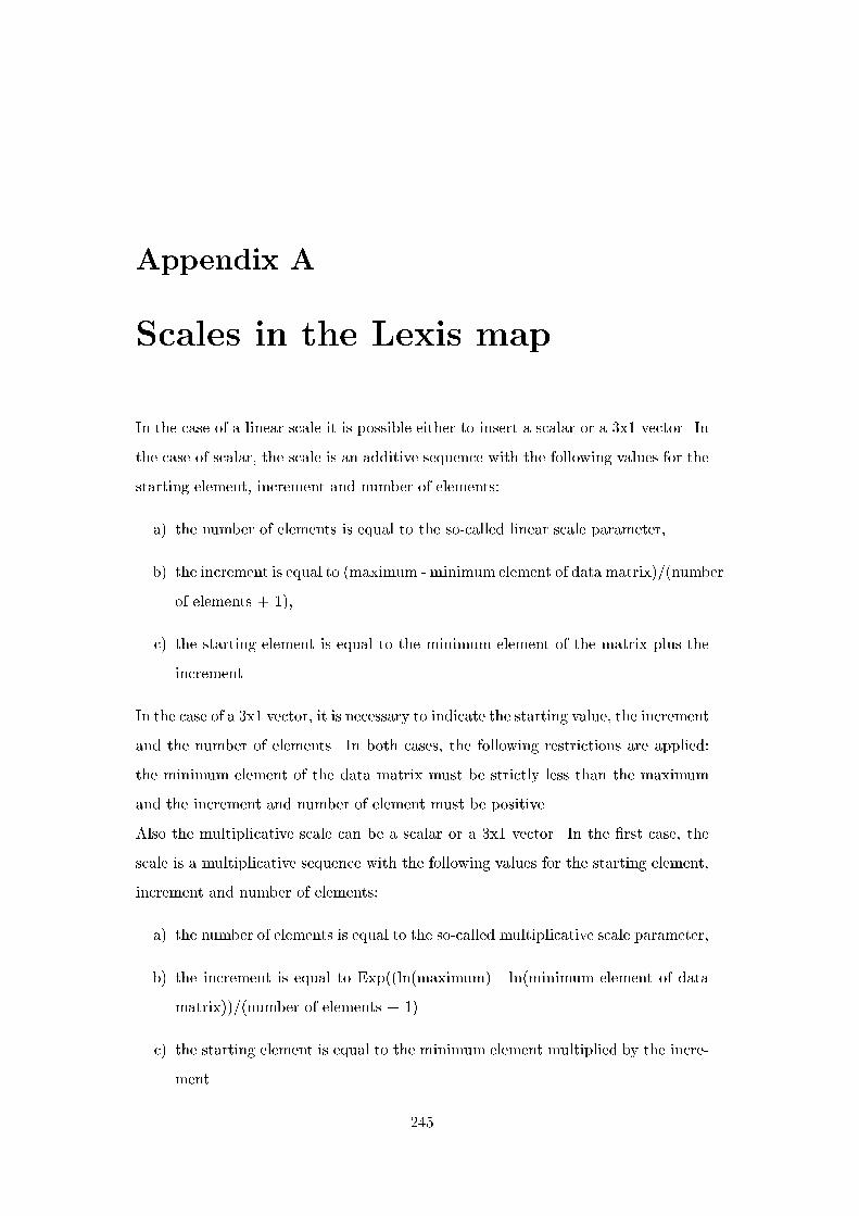
Appendix A
Scales in the Lexis map
In the case of a linear scale it is possible either to insert a scalar or a 3x1 vector. In
the case of scalar, the scale is an additive sequence with the following values for the
starting element, increment and number of elements:
a) the number of elements is equal to the so-called linear scale parameter,
b) the increment is equal to (maximum - minimum element of data matrix)/(number
of elements + 1),
c) the starting element is equal to the minimum element of the matrix plus the
increment.
In the case of a 3x1 vector, it is necessary to indicate the starting value, the increment
and the number of elements. In both cases, the following restrictions are applied:
the minimum element of the data matrix must be strictly less than the maximum
and the increment and number of element must be positive.
Also the multiplicative scale can be a scalar or a 3x1 vector. In the �rst case, the
scale is a multiplicative sequence with the following values for the starting element,
increment and number of elements:
a) the number of elements is equal to the so-called multiplicative scale parameter,
b) the increment is equal to Exp((ln(maximum) - ln(minimum element of data
matrix))/(number of elements + 1)
c) the starting element is equal to the minimum element multiplied by the incre-
ment.
245
246 Appendix A. Scales in the Lexis map
In the case of a 3x1 vector, it is necessary to indicate the starting value, the factor
and the number of elements. In both cases, the following restrictions are applied:
the minimum element of the data matrix must be strictly less than the maximum
element; the matrix value must be strictly positive, no zeros allowed; the factor must
be greater than one; and number of elements must be greater than zero.
Appendix B
Nuptiality tables
B.1 The nuptiality table
As described in the previous chapter, the Italian data-base for the years 1969-1995
contains the unconditional �rst marriage rates while, Schoen's indexes of marriage
market are based on occurrence-exposure rates of �rst marriage. Therefore, it is �rst
necessary to transform the unconditional rates into the probability of �rst marriage
for those still single at each age: to this aim we need to calculate the conditional rates
by dividing the number of marriages for each age and sex by the person-years lived
by the population at risk. To this aim one would need the population distribution
by marital status, which is available at the time of a census. A reconstruction
of the population distribution by marital status, age and sex is available for the
inter-censual period and at the national level for the years 1952-1981 (Castiglioni,
1989[43]). Yet, this reconstruction can not be used for building of the denominator
of the conditional rates of �rst marriage at regional level, which represents what we
need.
It is then necessary to pursue a di�erent strategy. In fact, in that case it is
possible to compute the person-years lived from age x and x+1 by those who are still
single at the beginning of the age group: this quantity represents the denominator
we are looking for.
For the sake of simplicity let us rename km(x; t) = mx, that represents the �rst
marriage rate for region of residence k, for spouses of each sex aged (x; x+1) during
year t. Starting from an initial birth cohort whose radix is l0 = 1000 people, all of
247
248 Appendix B. Nuptiality tables
them singles at age 15:
S0 = l0m0 (B.1)
represents, for the �rst age, the number of marriages of males (or females) aged 15.
At the beginning of the following year, those who are at risk of marrying will be
given by the di�erence:
l1 = l0 � S0 (B.2)
Then, for subsequent ages we should apply the rate of �rst marriage to those still
single at the beginning of age x:
Sx = lxmx (B.3)
is the number of marriages contracted from exact age x and exact age x+1 by those
still single at the beginning of that age, and therefore the number of survivors to
marriage at age x+ 1 is given by:
lx+1 = lx � Sx (B.4)
Now, one should also note that our starting unconditional �rst marriage rate, is a
rate comparable to that of a rectangular population:
mx =Mx
l0(B.5)
where Mx is the number of marriages at age x and l0 is the radix of the table, as
usual, but in this particular case is the same for every age. Therefore, to build
the new probability of marrying at age x one should need to divide the number of
marriages in the age group (x; x+1) of a nuptiality table by those who survive single
at the beginning of age x:
nx =Mx
lx=Mx
l0
l0
lx(B.6)
Therefore, once computed the survivors to marriage at age x, it is easy to adjust
the unconditional �rst marriage rates (B.5) by substituting the coe�cient:
cx =l0
lx(B.7)
in equation (B.6):
nx = mxcx (B.8)
B.1. The nuptiality table 249
Then, nx represents the conditional probability of marriage from age x to age x+1
and its complementary value 1 � nx represents the probability of remaining single
from age x to age x+ 1. Starting from a cohort radix equal to l0
0 = 1000 at age 15,
the survivors to the next age are given by:
l0
x+1 = l0
x(1� nx) (B.9)
which shows that to build a nuptiality table, it is necessary to apply the comple-
mentary values of (B.6) to unity, to the survivors in the status of single at each
age.
Therefore, basic elements of the nuptiality tables are: the survivors at marriage
l0
x (B.9), the conditional probability between exact ages, nx (B.6), the number of
marriages at each age given by multiplying l0
x by nx:
S0
x = l0
xnx (B.10)
It is now possible to compute the rate of �rst marriage in two di�erent way: on one
hand, assuming that marriages are linearly or uniformly distributed over the age
group x to x+ 1, by using the following formula:
�x =S
0
x
l0
x �12S
0
x
On the other hand, under the assumption that the rate are constant in the age
group, one can calculate the rate in continuous time, as the following relation holds:
nx = 1� e��x (B.11)
thus, by rearranging,
�x = �log(1� nx) (B.12)
where nx is the occurrence/exposure rate1.
B.1.1 Building the nuptiality tables for Italy, 1969-1995
The procedure described up to now has been applied to our data so that nuptiality
tables for every region and year and for both sexes, have been computed. In this
1One should also note that the sum over the ages of the conditional probabilities is not directly
interpretable, while reduced events are additive (Leridon and Toulemon, 1992, p.92[121]).
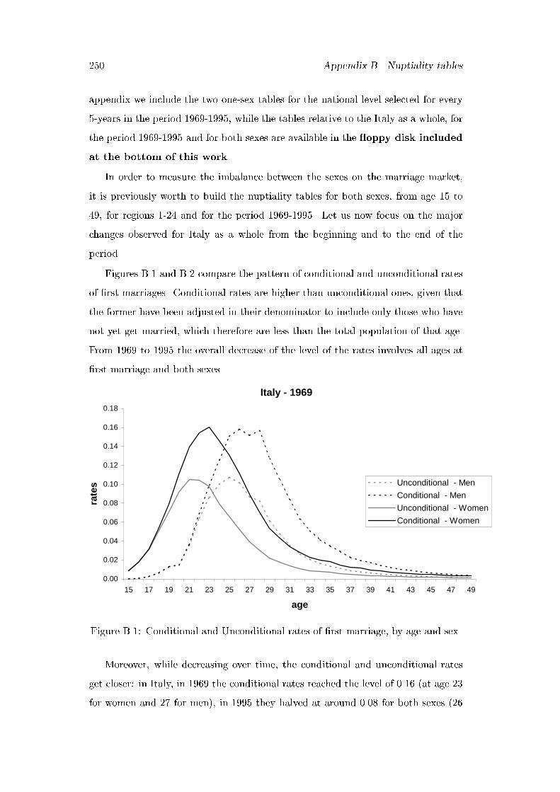
250 Appendix B. Nuptiality tables
appendix we include the two one-sex tables for the national level selected for every
5-years in the period 1969-1995, while the tables relative to the Italy as a whole, for
the period 1969-1995 and for both sexes are available in the oppy disk included
at the bottom of this work.
In order to measure the imbalance between the sexes on the marriage market,
it is previously worth to build the nuptiality tables for both sexes, from age 15 to
49, for regions 1-24 and for the period 1969-1995. Let us now focus on the major
changes observed for Italy as a whole from the beginning and to the end of the
period.
Figures B.1 and B.2 compare the pattern of conditional and unconditional rates
of �rst marriages. Conditional rates are higher than unconditional ones, given that
the former have been adjusted in their denominator to include only those who have
not yet get married, which therefore are less than the total population of that age.
From 1969 to 1995 the overall decrease of the level of the rates involves all ages at
�rst marriage and both sexes.
Italy - 1969
0.00
0.02
0.04
0.06
0.08
0.10
0.12
0.14
0.16
0.18
15 17 19 21 23 25 27 29 31 33 35 37 39 41 43 45 47 49
age
rate
s Unconditional - Men
Conditional - Men
Unconditional - Women
Conditional - Women
Figure B.1: Conditional and Unconditional rates of �rst marriage, by age and sex.
Moreover, while decreasing over time, the conditional and unconditional rates
get closer: in Italy, in 1969 the conditional rates reached the level of 0.16 (at age 23
for women and 27 for men), in 1995 they halved at around 0.08 for both sexes (26

B.1. The nuptiality table 251
for women and 28 for men), while, during the same period, the unconditional rates
declined from a maximum of 0.10 in 1969 (at age 21 for women and 25 for men)
to a maximum of about 0.06 (at age 25 for women, and 28 for men). Of course,
one should also note the postponement of the timing of �rst marriage pattern in 25
years of observation.
Italy - 1995
0.00
0.02
0.04
0.06
0.08
0.10
0.12
0.14
0.16
0.18
15 17 19 21 23 25 27 29 31 33 35 37 39 41 43 45 47 49
age
rate
s Unconditional - Men
Conditional - Men
Unconditional Women
Conditional -Women
Figure B.2: Conditional and Unconditional rates of �rst marriage, by age and sex.
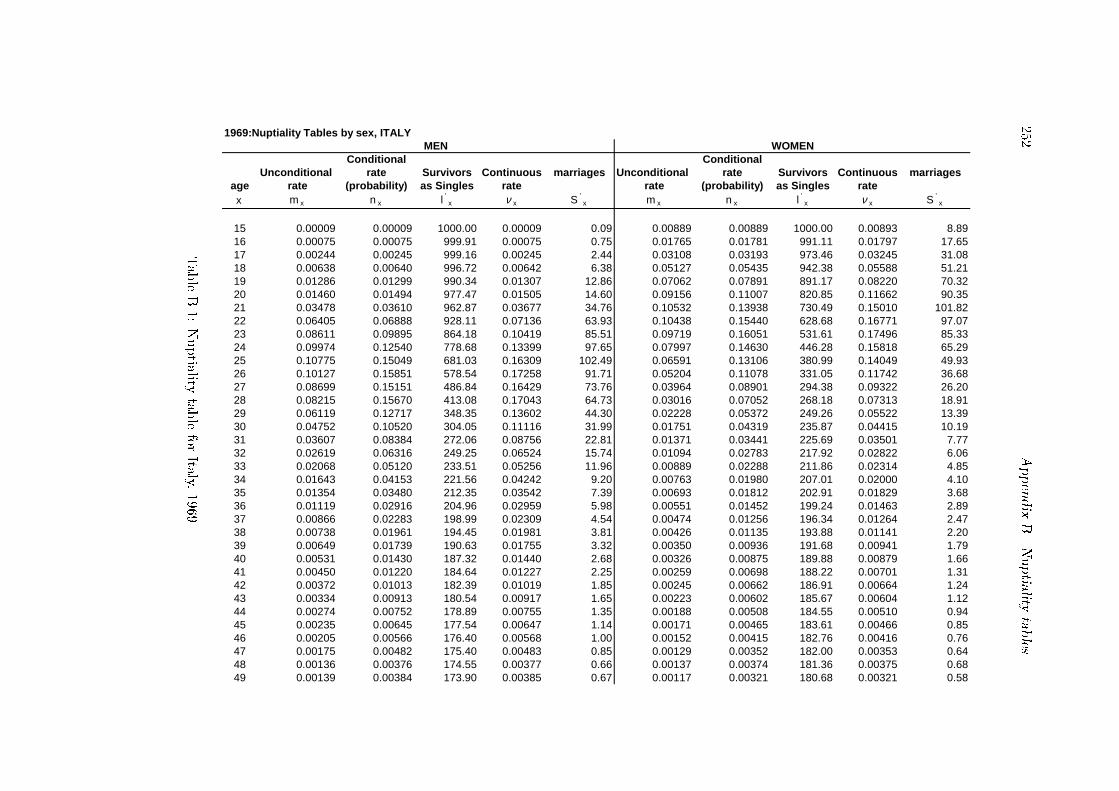
252
Appendix
B.Nuptia
litytables
1969:Nuptiality Tables by sex, ITALY
Conditional ConditionalUnconditional rate Survivors Continuous marriages Unconditional rate Survivors Continuous marriages
age rate (probability) as Singles rate rate (probability) as Singles ratex m x n x l '
x ν x S 'x m x n x l '
x ν x S 'x
15 0.00009 0.00009 1000.00 0.00009 0.09 0.00889 0.00889 1000.00 0.00893 8.8916 0.00075 0.00075 999.91 0.00075 0.75 0.01765 0.01781 991.11 0.01797 17.6517 0.00244 0.00245 999.16 0.00245 2.44 0.03108 0.03193 973.46 0.03245 31.0818 0.00638 0.00640 996.72 0.00642 6.38 0.05127 0.05435 942.38 0.05588 51.2119 0.01286 0.01299 990.34 0.01307 12.86 0.07062 0.07891 891.17 0.08220 70.3220 0.01460 0.01494 977.47 0.01505 14.60 0.09156 0.11007 820.85 0.11662 90.3521 0.03478 0.03610 962.87 0.03677 34.76 0.10532 0.13938 730.49 0.15010 101.8222 0.06405 0.06888 928.11 0.07136 63.93 0.10438 0.15440 628.68 0.16771 97.0723 0.08611 0.09895 864.18 0.10419 85.51 0.09719 0.16051 531.61 0.17496 85.3324 0.09974 0.12540 778.68 0.13399 97.65 0.07997 0.14630 446.28 0.15818 65.2925 0.10775 0.15049 681.03 0.16309 102.49 0.06591 0.13106 380.99 0.14049 49.9326 0.10127 0.15851 578.54 0.17258 91.71 0.05204 0.11078 331.05 0.11742 36.6827 0.08699 0.15151 486.84 0.16429 73.76 0.03964 0.08901 294.38 0.09322 26.2028 0.08215 0.15670 413.08 0.17043 64.73 0.03016 0.07052 268.18 0.07313 18.9129 0.06119 0.12717 348.35 0.13602 44.30 0.02228 0.05372 249.26 0.05522 13.3930 0.04752 0.10520 304.05 0.11116 31.99 0.01751 0.04319 235.87 0.04415 10.1931 0.03607 0.08384 272.06 0.08756 22.81 0.01371 0.03441 225.69 0.03501 7.7732 0.02619 0.06316 249.25 0.06524 15.74 0.01094 0.02783 217.92 0.02822 6.0633 0.02068 0.05120 233.51 0.05256 11.96 0.00889 0.02288 211.86 0.02314 4.8534 0.01643 0.04153 221.56 0.04242 9.20 0.00763 0.01980 207.01 0.02000 4.1035 0.01354 0.03480 212.35 0.03542 7.39 0.00693 0.01812 202.91 0.01829 3.6836 0.01119 0.02916 204.96 0.02959 5.98 0.00551 0.01452 199.24 0.01463 2.8937 0.00866 0.02283 198.99 0.02309 4.54 0.00474 0.01256 196.34 0.01264 2.4738 0.00738 0.01961 194.45 0.01981 3.81 0.00426 0.01135 193.88 0.01141 2.2039 0.00649 0.01739 190.63 0.01755 3.32 0.00350 0.00936 191.68 0.00941 1.7940 0.00531 0.01430 187.32 0.01440 2.68 0.00326 0.00875 189.88 0.00879 1.6641 0.00450 0.01220 184.64 0.01227 2.25 0.00259 0.00698 188.22 0.00701 1.3142 0.00372 0.01013 182.39 0.01019 1.85 0.00245 0.00662 186.91 0.00664 1.2443 0.00334 0.00913 180.54 0.00917 1.65 0.00223 0.00602 185.67 0.00604 1.1244 0.00274 0.00752 178.89 0.00755 1.35 0.00188 0.00508 184.55 0.00510 0.9445 0.00235 0.00645 177.54 0.00647 1.14 0.00171 0.00465 183.61 0.00466 0.8546 0.00205 0.00566 176.40 0.00568 1.00 0.00152 0.00415 182.76 0.00416 0.7647 0.00175 0.00482 175.40 0.00483 0.85 0.00129 0.00352 182.00 0.00353 0.6448 0.00136 0.00376 174.55 0.00377 0.66 0.00137 0.00374 181.36 0.00375 0.6849 0.00139 0.00384 173.90 0.00385 0.67 0.00117 0.00321 180.68 0.00321 0.58
MEN WOMEN
TableB.1:Nuptia
litytableforIta
ly,1969
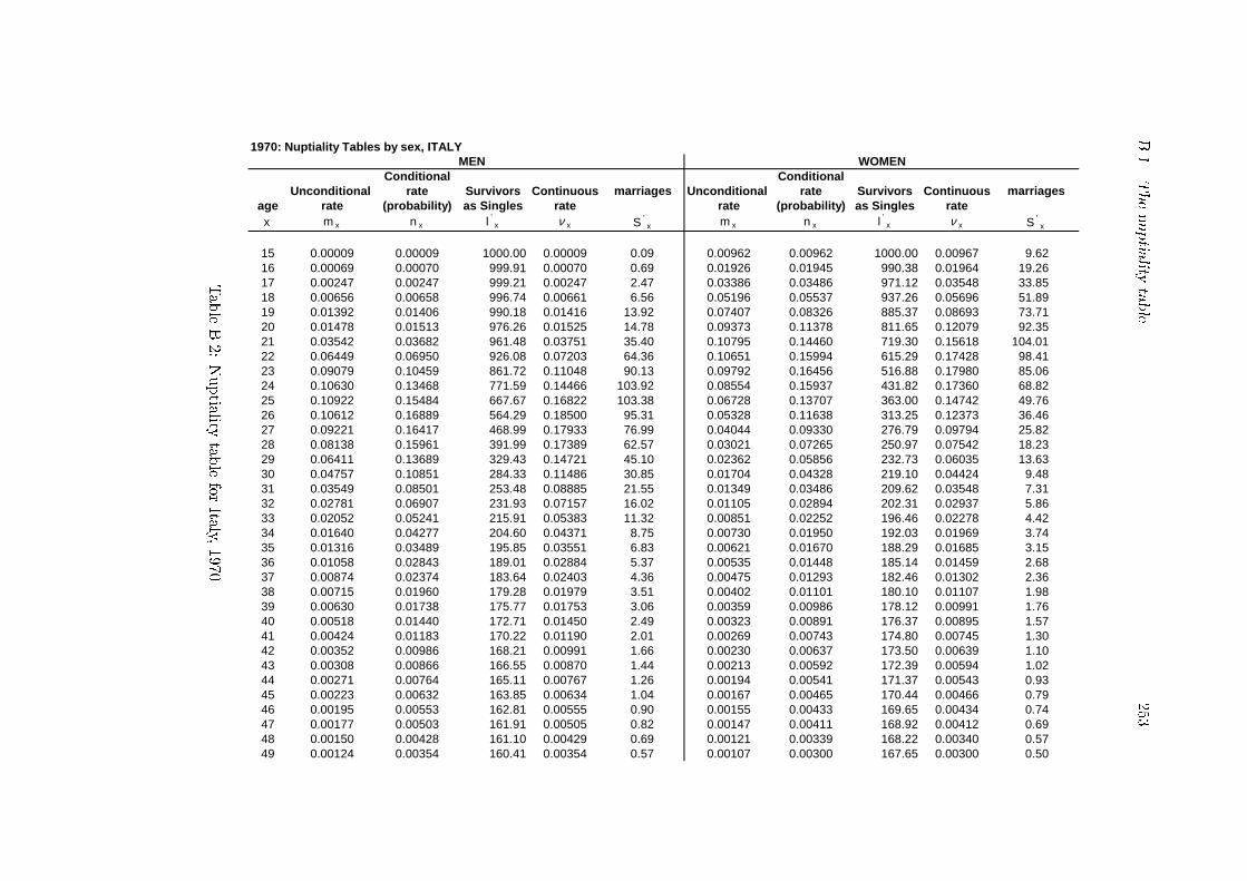
B.1.Thenuptia
litytable
253
1970: Nuptiality Tables by sex, ITALY
Conditional ConditionalUnconditional rate Survivors Continuous Unconditional rate Survivors Continuous
age rate (probability) as Singles rate rate (probability) as Singles ratex m x n x l '
x ν x m x n x l 'x ν x
15 0.00009 0.00009 1000.00 0.00009 0.09 0.00962 0.00962 1000.00 0.00967 9.6216 0.00069 0.00070 999.91 0.00070 0.69 0.01926 0.01945 990.38 0.01964 19.2617 0.00247 0.00247 999.21 0.00247 2.47 0.03386 0.03486 971.12 0.03548 33.8518 0.00656 0.00658 996.74 0.00661 6.56 0.05196 0.05537 937.26 0.05696 51.8919 0.01392 0.01406 990.18 0.01416 13.92 0.07407 0.08326 885.37 0.08693 73.7120 0.01478 0.01513 976.26 0.01525 14.78 0.09373 0.11378 811.65 0.12079 92.3521 0.03542 0.03682 961.48 0.03751 35.40 0.10795 0.14460 719.30 0.15618 104.0122 0.06449 0.06950 926.08 0.07203 64.36 0.10651 0.15994 615.29 0.17428 98.4123 0.09079 0.10459 861.72 0.11048 90.13 0.09792 0.16456 516.88 0.17980 85.0624 0.10630 0.13468 771.59 0.14466 103.92 0.08554 0.15937 431.82 0.17360 68.8225 0.10922 0.15484 667.67 0.16822 103.38 0.06728 0.13707 363.00 0.14742 49.7626 0.10612 0.16889 564.29 0.18500 95.31 0.05328 0.11638 313.25 0.12373 36.4627 0.09221 0.16417 468.99 0.17933 76.99 0.04044 0.09330 276.79 0.09794 25.8228 0.08138 0.15961 391.99 0.17389 62.57 0.03021 0.07265 250.97 0.07542 18.2329 0.06411 0.13689 329.43 0.14721 45.10 0.02362 0.05856 232.73 0.06035 13.6330 0.04757 0.10851 284.33 0.11486 30.85 0.01704 0.04328 219.10 0.04424 9.4831 0.03549 0.08501 253.48 0.08885 21.55 0.01349 0.03486 209.62 0.03548 7.3132 0.02781 0.06907 231.93 0.07157 16.02 0.01105 0.02894 202.31 0.02937 5.8633 0.02052 0.05241 215.91 0.05383 11.32 0.00851 0.02252 196.46 0.02278 4.4234 0.01640 0.04277 204.60 0.04371 8.75 0.00730 0.01950 192.03 0.01969 3.7435 0.01316 0.03489 195.85 0.03551 6.83 0.00621 0.01670 188.29 0.01685 3.1536 0.01058 0.02843 189.01 0.02884 5.37 0.00535 0.01448 185.14 0.01459 2.6837 0.00874 0.02374 183.64 0.02403 4.36 0.00475 0.01293 182.46 0.01302 2.3638 0.00715 0.01960 179.28 0.01979 3.51 0.00402 0.01101 180.10 0.01107 1.9839 0.00630 0.01738 175.77 0.01753 3.06 0.00359 0.00986 178.12 0.00991 1.7640 0.00518 0.01440 172.71 0.01450 2.49 0.00323 0.00891 176.37 0.00895 1.5741 0.00424 0.01183 170.22 0.01190 2.01 0.00269 0.00743 174.80 0.00745 1.3042 0.00352 0.00986 168.21 0.00991 1.66 0.00230 0.00637 173.50 0.00639 1.1043 0.00308 0.00866 166.55 0.00870 1.44 0.00213 0.00592 172.39 0.00594 1.0244 0.00271 0.00764 165.11 0.00767 1.26 0.00194 0.00541 171.37 0.00543 0.9345 0.00223 0.00632 163.85 0.00634 1.04 0.00167 0.00465 170.44 0.00466 0.7946 0.00195 0.00553 162.81 0.00555 0.90 0.00155 0.00433 169.65 0.00434 0.7447 0.00177 0.00503 161.91 0.00505 0.82 0.00147 0.00411 168.92 0.00412 0.6948 0.00150 0.00428 161.10 0.00429 0.69 0.00121 0.00339 168.22 0.00340 0.5749 0.00124 0.00354 160.41 0.00354 0.57 0.00107 0.00300 167.65 0.00300 0.50
MEN WOMEN
marriages marriages
S 'x S '
x
TableB.2:Nuptia
litytableforIta
ly,1970
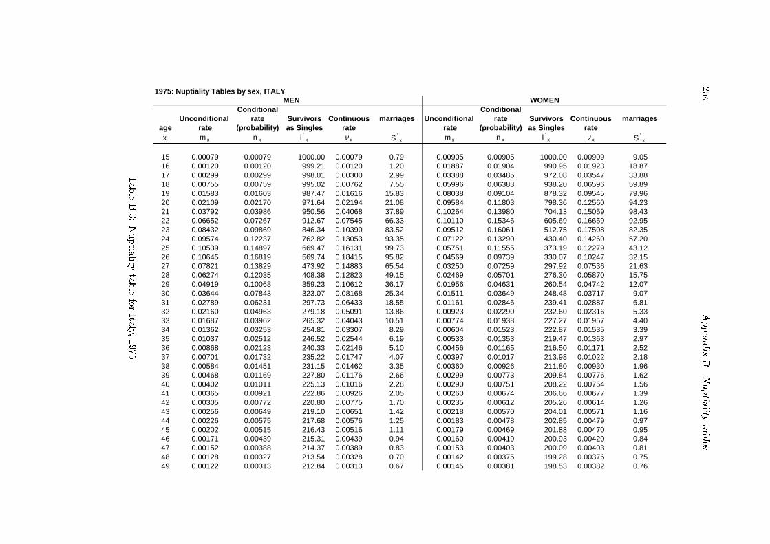
254
Appendix
B.Nuptia
litytables
1975: Nuptiality Tables by sex, ITALY
Conditional ConditionalUnconditional rate Survivors Continuous Unconditional rate Survivors Continuous
age rate (probability) as Singles rate rate (probability) as Singles ratex m x n x l '
x ν x m x n x l 'x ν x
15 0.00079 0.00079 1000.00 0.00079 0.79 0.00905 0.00905 1000.00 0.00909 9.0516 0.00120 0.00120 999.21 0.00120 1.20 0.01887 0.01904 990.95 0.01923 18.8717 0.00299 0.00299 998.01 0.00300 2.99 0.03388 0.03485 972.08 0.03547 33.8818 0.00755 0.00759 995.02 0.00762 7.55 0.05996 0.06383 938.20 0.06596 59.8919 0.01583 0.01603 987.47 0.01616 15.83 0.08038 0.09104 878.32 0.09545 79.9620 0.02109 0.02170 971.64 0.02194 21.08 0.09584 0.11803 798.36 0.12560 94.2321 0.03792 0.03986 950.56 0.04068 37.89 0.10264 0.13980 704.13 0.15059 98.4322 0.06652 0.07267 912.67 0.07545 66.33 0.10110 0.15346 605.69 0.16659 92.9523 0.08432 0.09869 846.34 0.10390 83.52 0.09512 0.16061 512.75 0.17508 82.3524 0.09574 0.12237 762.82 0.13053 93.35 0.07122 0.13290 430.40 0.14260 57.2025 0.10539 0.14897 669.47 0.16131 99.73 0.05751 0.11555 373.19 0.12279 43.1226 0.10645 0.16819 569.74 0.18415 95.82 0.04569 0.09739 330.07 0.10247 32.1527 0.07821 0.13829 473.92 0.14883 65.54 0.03250 0.07259 297.92 0.07536 21.6328 0.06274 0.12035 408.38 0.12823 49.15 0.02469 0.05701 276.30 0.05870 15.7529 0.04919 0.10068 359.23 0.10612 36.17 0.01956 0.04631 260.54 0.04742 12.0730 0.03644 0.07843 323.07 0.08168 25.34 0.01511 0.03649 248.48 0.03717 9.0731 0.02789 0.06231 297.73 0.06433 18.55 0.01161 0.02846 239.41 0.02887 6.8132 0.02160 0.04963 279.18 0.05091 13.86 0.00923 0.02290 232.60 0.02316 5.3333 0.01687 0.03962 265.32 0.04043 10.51 0.00774 0.01938 227.27 0.01957 4.4034 0.01362 0.03253 254.81 0.03307 8.29 0.00604 0.01523 222.87 0.01535 3.3935 0.01037 0.02512 246.52 0.02544 6.19 0.00533 0.01353 219.47 0.01363 2.9736 0.00868 0.02123 240.33 0.02146 5.10 0.00456 0.01165 216.50 0.01171 2.5237 0.00701 0.01732 235.22 0.01747 4.07 0.00397 0.01017 213.98 0.01022 2.1838 0.00584 0.01451 231.15 0.01462 3.35 0.00360 0.00926 211.80 0.00930 1.9639 0.00468 0.01169 227.80 0.01176 2.66 0.00299 0.00773 209.84 0.00776 1.6240 0.00402 0.01011 225.13 0.01016 2.28 0.00290 0.00751 208.22 0.00754 1.5641 0.00365 0.00921 222.86 0.00926 2.05 0.00260 0.00674 206.66 0.00677 1.3942 0.00305 0.00772 220.80 0.00775 1.70 0.00235 0.00612 205.26 0.00614 1.2643 0.00256 0.00649 219.10 0.00651 1.42 0.00218 0.00570 204.01 0.00571 1.1644 0.00226 0.00575 217.68 0.00576 1.25 0.00183 0.00478 202.85 0.00479 0.9745 0.00202 0.00515 216.43 0.00516 1.11 0.00179 0.00469 201.88 0.00470 0.9546 0.00171 0.00439 215.31 0.00439 0.94 0.00160 0.00419 200.93 0.00420 0.8447 0.00152 0.00388 214.37 0.00389 0.83 0.00153 0.00403 200.09 0.00403 0.8148 0.00128 0.00327 213.54 0.00328 0.70 0.00142 0.00375 199.28 0.00376 0.7549 0.00122 0.00313 212.84 0.00313 0.67 0.00145 0.00381 198.53 0.00382 0.76
marriages marriages
S 'x S '
x
MEN WOMEN
TableB.3:Nuptia
litytableforIta
ly,1975
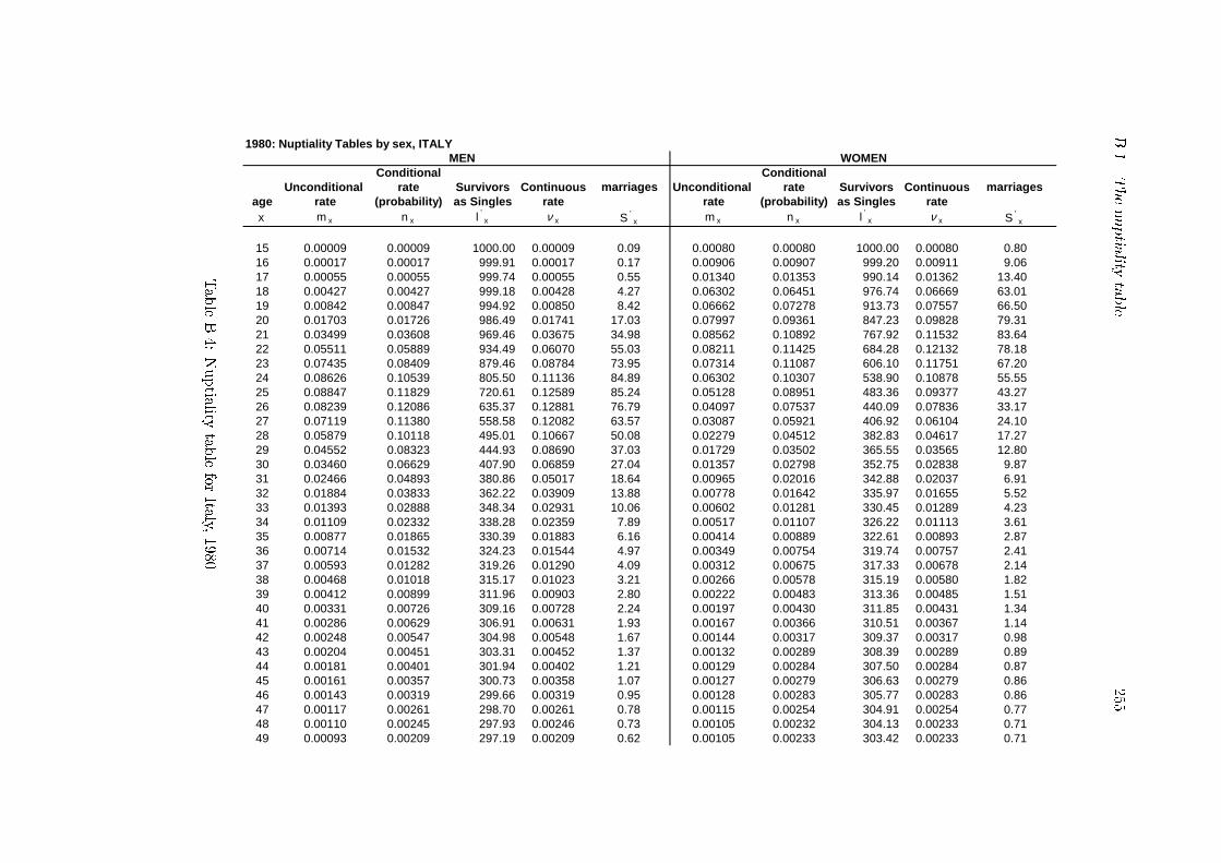
B.1.Thenuptia
litytable
255
1980: Nuptiality Tables by sex, ITALY
Conditional ConditionalUnconditional rate Survivors Continuous Unconditional rate Survivors Continuous
age rate (probability) as Singles rate rate (probability) as Singles ratex m x n x l '
x ν x m x n x l 'x ν x
15 0.00009 0.00009 1000.00 0.00009 0.09 0.00080 0.00080 1000.00 0.00080 0.8016 0.00017 0.00017 999.91 0.00017 0.17 0.00906 0.00907 999.20 0.00911 9.0617 0.00055 0.00055 999.74 0.00055 0.55 0.01340 0.01353 990.14 0.01362 13.4018 0.00427 0.00427 999.18 0.00428 4.27 0.06302 0.06451 976.74 0.06669 63.0119 0.00842 0.00847 994.92 0.00850 8.42 0.06662 0.07278 913.73 0.07557 66.5020 0.01703 0.01726 986.49 0.01741 17.03 0.07997 0.09361 847.23 0.09828 79.3121 0.03499 0.03608 969.46 0.03675 34.98 0.08562 0.10892 767.92 0.11532 83.6422 0.05511 0.05889 934.49 0.06070 55.03 0.08211 0.11425 684.28 0.12132 78.1823 0.07435 0.08409 879.46 0.08784 73.95 0.07314 0.11087 606.10 0.11751 67.2024 0.08626 0.10539 805.50 0.11136 84.89 0.06302 0.10307 538.90 0.10878 55.5525 0.08847 0.11829 720.61 0.12589 85.24 0.05128 0.08951 483.36 0.09377 43.2726 0.08239 0.12086 635.37 0.12881 76.79 0.04097 0.07537 440.09 0.07836 33.1727 0.07119 0.11380 558.58 0.12082 63.57 0.03087 0.05921 406.92 0.06104 24.1028 0.05879 0.10118 495.01 0.10667 50.08 0.02279 0.04512 382.83 0.04617 17.2729 0.04552 0.08323 444.93 0.08690 37.03 0.01729 0.03502 365.55 0.03565 12.8030 0.03460 0.06629 407.90 0.06859 27.04 0.01357 0.02798 352.75 0.02838 9.8731 0.02466 0.04893 380.86 0.05017 18.64 0.00965 0.02016 342.88 0.02037 6.9132 0.01884 0.03833 362.22 0.03909 13.88 0.00778 0.01642 335.97 0.01655 5.5233 0.01393 0.02888 348.34 0.02931 10.06 0.00602 0.01281 330.45 0.01289 4.2334 0.01109 0.02332 338.28 0.02359 7.89 0.00517 0.01107 326.22 0.01113 3.6135 0.00877 0.01865 330.39 0.01883 6.16 0.00414 0.00889 322.61 0.00893 2.8736 0.00714 0.01532 324.23 0.01544 4.97 0.00349 0.00754 319.74 0.00757 2.4137 0.00593 0.01282 319.26 0.01290 4.09 0.00312 0.00675 317.33 0.00678 2.1438 0.00468 0.01018 315.17 0.01023 3.21 0.00266 0.00578 315.19 0.00580 1.8239 0.00412 0.00899 311.96 0.00903 2.80 0.00222 0.00483 313.36 0.00485 1.5140 0.00331 0.00726 309.16 0.00728 2.24 0.00197 0.00430 311.85 0.00431 1.3441 0.00286 0.00629 306.91 0.00631 1.93 0.00167 0.00366 310.51 0.00367 1.1442 0.00248 0.00547 304.98 0.00548 1.67 0.00144 0.00317 309.37 0.00317 0.9843 0.00204 0.00451 303.31 0.00452 1.37 0.00132 0.00289 308.39 0.00289 0.8944 0.00181 0.00401 301.94 0.00402 1.21 0.00129 0.00284 307.50 0.00284 0.8745 0.00161 0.00357 300.73 0.00358 1.07 0.00127 0.00279 306.63 0.00279 0.8646 0.00143 0.00319 299.66 0.00319 0.95 0.00128 0.00283 305.77 0.00283 0.8647 0.00117 0.00261 298.70 0.00261 0.78 0.00115 0.00254 304.91 0.00254 0.7748 0.00110 0.00245 297.93 0.00246 0.73 0.00105 0.00232 304.13 0.00233 0.7149 0.00093 0.00209 297.19 0.00209 0.62 0.00105 0.00233 303.42 0.00233 0.71
MEN WOMEN
marriages marriages
S 'x S '
x
TableB.4:Nuptia
litytableforIta
ly,1980
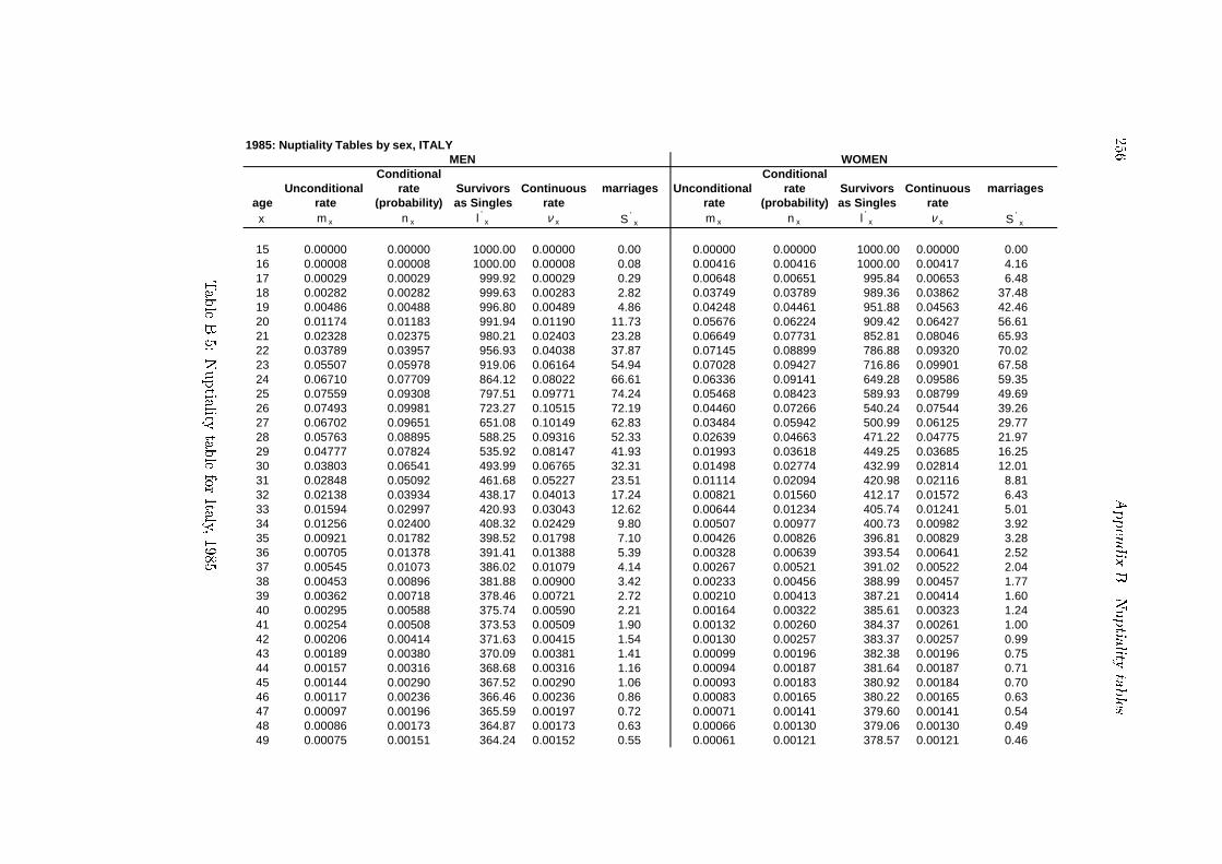
256
Appendix
B.Nuptia
litytables
1985: Nuptiality Tables by sex, ITALY
Conditional ConditionalUnconditional rate Survivors Continuous Unconditional rate Survivors Continuous
age rate (probability) as Singles rate rate (probability) as Singles ratex m x n x l '
x ν x m x n x l 'x ν x
15 0.00000 0.00000 1000.00 0.00000 0.00 0.00000 0.00000 1000.00 0.00000 0.0016 0.00008 0.00008 1000.00 0.00008 0.08 0.00416 0.00416 1000.00 0.00417 4.1617 0.00029 0.00029 999.92 0.00029 0.29 0.00648 0.00651 995.84 0.00653 6.4818 0.00282 0.00282 999.63 0.00283 2.82 0.03749 0.03789 989.36 0.03862 37.4819 0.00486 0.00488 996.80 0.00489 4.86 0.04248 0.04461 951.88 0.04563 42.4620 0.01174 0.01183 991.94 0.01190 11.73 0.05676 0.06224 909.42 0.06427 56.6121 0.02328 0.02375 980.21 0.02403 23.28 0.06649 0.07731 852.81 0.08046 65.9322 0.03789 0.03957 956.93 0.04038 37.87 0.07145 0.08899 786.88 0.09320 70.0223 0.05507 0.05978 919.06 0.06164 54.94 0.07028 0.09427 716.86 0.09901 67.5824 0.06710 0.07709 864.12 0.08022 66.61 0.06336 0.09141 649.28 0.09586 59.3525 0.07559 0.09308 797.51 0.09771 74.24 0.05468 0.08423 589.93 0.08799 49.6926 0.07493 0.09981 723.27 0.10515 72.19 0.04460 0.07266 540.24 0.07544 39.2627 0.06702 0.09651 651.08 0.10149 62.83 0.03484 0.05942 500.99 0.06125 29.7728 0.05763 0.08895 588.25 0.09316 52.33 0.02639 0.04663 471.22 0.04775 21.9729 0.04777 0.07824 535.92 0.08147 41.93 0.01993 0.03618 449.25 0.03685 16.2530 0.03803 0.06541 493.99 0.06765 32.31 0.01498 0.02774 432.99 0.02814 12.0131 0.02848 0.05092 461.68 0.05227 23.51 0.01114 0.02094 420.98 0.02116 8.8132 0.02138 0.03934 438.17 0.04013 17.24 0.00821 0.01560 412.17 0.01572 6.4333 0.01594 0.02997 420.93 0.03043 12.62 0.00644 0.01234 405.74 0.01241 5.0134 0.01256 0.02400 408.32 0.02429 9.80 0.00507 0.00977 400.73 0.00982 3.9235 0.00921 0.01782 398.52 0.01798 7.10 0.00426 0.00826 396.81 0.00829 3.2836 0.00705 0.01378 391.41 0.01388 5.39 0.00328 0.00639 393.54 0.00641 2.5237 0.00545 0.01073 386.02 0.01079 4.14 0.00267 0.00521 391.02 0.00522 2.0438 0.00453 0.00896 381.88 0.00900 3.42 0.00233 0.00456 388.99 0.00457 1.7739 0.00362 0.00718 378.46 0.00721 2.72 0.00210 0.00413 387.21 0.00414 1.6040 0.00295 0.00588 375.74 0.00590 2.21 0.00164 0.00322 385.61 0.00323 1.2441 0.00254 0.00508 373.53 0.00509 1.90 0.00132 0.00260 384.37 0.00261 1.0042 0.00206 0.00414 371.63 0.00415 1.54 0.00130 0.00257 383.37 0.00257 0.9943 0.00189 0.00380 370.09 0.00381 1.41 0.00099 0.00196 382.38 0.00196 0.7544 0.00157 0.00316 368.68 0.00316 1.16 0.00094 0.00187 381.64 0.00187 0.7145 0.00144 0.00290 367.52 0.00290 1.06 0.00093 0.00183 380.92 0.00184 0.7046 0.00117 0.00236 366.46 0.00236 0.86 0.00083 0.00165 380.22 0.00165 0.6347 0.00097 0.00196 365.59 0.00197 0.72 0.00071 0.00141 379.60 0.00141 0.5448 0.00086 0.00173 364.87 0.00173 0.63 0.00066 0.00130 379.06 0.00130 0.4949 0.00075 0.00151 364.24 0.00152 0.55 0.00061 0.00121 378.57 0.00121 0.46
marriages marriages
S 'x S '
x
MEN WOMEN
TableB.5:Nuptia
litytableforIta
ly,1985
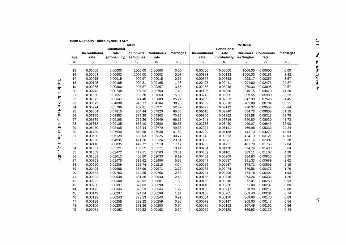
B.1.Thenuptia
litytable
257
1990: Nuptiality Tables by sex, ITALY
Conditional ConditionalUnconditional rate Survivors Continuous Unconditional rate Survivors Continuous
age rate (probability) as Singles rate rate (probability) as Singles ratex m x n x l '
x ν x m x n x l 'x ν x
15 0.00000 0.00000 1000.00 0.00000 0.00 0.00000 0.00000 1000.00 0.00000 0.0016 0.00003 0.00003 1000.00 0.00003 0.03 0.00183 0.00183 1000.00 0.00183 1.8317 0.00015 0.00015 999.97 0.00015 0.15 0.00357 0.00358 998.17 0.00359 3.5718 0.00195 0.00195 999.81 0.00195 1.95 0.02427 0.02441 994.60 0.02471 24.2719 0.00365 0.00366 997.87 0.00367 3.65 0.02958 0.03048 970.33 0.03095 29.5720 0.00743 0.00748 994.22 0.00750 7.43 0.04125 0.04380 940.75 0.04479 41.2021 0.01530 0.01551 986.78 0.01563 15.30 0.05242 0.05805 899.55 0.05980 52.2222 0.02572 0.02647 971.48 0.02683 25.71 0.06205 0.07253 847.33 0.07529 61.4523 0.03879 0.04098 945.77 0.04184 38.75 0.06689 0.08336 785.88 0.08704 65.5124 0.05274 0.05796 907.01 0.05971 52.57 0.06823 0.09112 720.37 0.09554 65.6425 0.06564 0.07615 854.44 0.07920 65.06 0.06516 0.09340 654.73 0.09805 61.1526 0.07155 0.08883 789.38 0.09303 70.12 0.05800 0.08892 593.58 0.09313 52.7827 0.06879 0.09198 719.26 0.09649 66.16 0.04741 0.07716 540.80 0.08030 41.7328 0.06362 0.09135 653.10 0.09580 59.66 0.03763 0.06430 499.07 0.06646 32.0929 0.05480 0.08405 593.44 0.08779 49.88 0.02924 0.05191 466.98 0.05331 24.2430 0.04709 0.07640 543.56 0.07948 41.53 0.02290 0.04188 442.73 0.04279 18.5431 0.03600 0.06129 502.03 0.06325 30.77 0.01642 0.03073 424.19 0.03121 13.0332 0.02828 0.04995 471.26 0.05124 23.54 0.01198 0.02281 411.16 0.02307 9.3833 0.02110 0.03835 447.72 0.03910 17.17 0.00909 0.01751 401.78 0.01766 7.0434 0.01681 0.03121 430.55 0.03171 13.44 0.00734 0.01428 394.74 0.01438 5.6435 0.01309 0.02472 417.11 0.02503 10.31 0.00562 0.01101 389.11 0.01107 4.2836 0.01052 0.02012 406.80 0.02033 8.19 0.00461 0.00909 384.83 0.00913 3.5037 0.00763 0.01475 398.62 0.01486 5.88 0.00347 0.00687 381.33 0.00689 2.6238 0.00620 0.01208 392.74 0.01215 4.74 0.00285 0.00567 378.71 0.00568 2.1539 0.00493 0.00966 387.99 0.00971 3.75 0.00238 0.00474 376.56 0.00475 1.7940 0.00382 0.00753 384.25 0.00755 2.89 0.00204 0.00406 374.78 0.00407 1.5241 0.00323 0.00638 381.35 0.00640 2.43 0.00168 0.00335 373.26 0.00336 1.2542 0.00252 0.00500 378.92 0.00501 1.89 0.00125 0.00249 372.01 0.00250 0.9343 0.00200 0.00397 377.03 0.00398 1.50 0.00118 0.00236 371.08 0.00237 0.8844 0.00172 0.00344 375.53 0.00344 1.29 0.00108 0.00217 370.20 0.00217 0.8045 0.00149 0.00297 374.24 0.00298 1.11 0.00100 0.00201 369.40 0.00201 0.7446 0.00122 0.00243 373.13 0.00243 0.91 0.00084 0.00170 368.66 0.00170 0.6347 0.00129 0.00258 372.22 0.00259 0.96 0.00073 0.00147 368.03 0.00147 0.5448 0.00100 0.00200 371.26 0.00200 0.74 0.00075 0.00152 367.49 0.00152 0.5649 0.00081 0.00163 370.52 0.00163 0.60 0.00059 0.00120 366.93 0.00120 0.44
MEN WOMEN
marriages marriages
S 'x S '
x
TableB.6:Nuptia
litytableforIta
ly,1990

258
Appendix
B.Nuptia
litytables
1995: Nuptiality Tables by sex, ITALY
Conditional ConditionalUnconditional rate Survivors Continuous Unconditional rate Survivors Continuous
age rate (probability) as Singles rate rate (probability) as Singles ratex m x n x l '
x ν x m x n x l 'x ν x
15 0.00000 0.00000 1000.00 0.00000 0.00 0.00000 0.00000 1000.00 0.00000 0.0016 0.00001 0.00001 1000.00 0.00001 0.01 0.00089 0.00089 1000.00 0.00089 0.8917 0.00011 0.00011 999.99 0.00011 0.11 0.00203 0.00203 999.11 0.00203 2.0318 0.00134 0.00134 999.88 0.00134 1.34 0.01510 0.01514 997.08 0.01526 15.1019 0.00252 0.00252 998.54 0.00252 2.52 0.01862 0.01896 981.99 0.01914 18.6220 0.00486 0.00487 996.03 0.00489 4.86 0.02587 0.02684 963.37 0.02721 25.8621 0.00864 0.00872 991.17 0.00876 8.64 0.03332 0.03549 937.51 0.03614 33.2822 0.01440 0.01466 982.53 0.01476 14.40 0.04181 0.04607 904.23 0.04716 41.6523 0.02174 0.02245 968.13 0.02271 21.74 0.05005 0.05755 862.58 0.05928 49.6424 0.03169 0.03345 946.39 0.03402 31.65 0.05694 0.06893 812.94 0.07142 56.0425 0.04371 0.04765 914.74 0.04882 43.58 0.05963 0.07655 756.90 0.07964 57.9426 0.05250 0.05984 871.16 0.06170 52.13 0.05790 0.07903 698.96 0.08233 55.2427 0.05756 0.06924 819.03 0.07176 56.71 0.05240 0.07593 643.72 0.07897 48.8828 0.05789 0.07390 762.32 0.07677 56.34 0.04436 0.06783 594.84 0.07024 40.3529 0.05443 0.07375 705.98 0.07661 52.07 0.03670 0.05873 554.49 0.06052 32.5630 0.04793 0.06869 653.91 0.07116 44.92 0.02888 0.04797 521.93 0.04916 25.0431 0.04023 0.06055 609.00 0.06246 36.87 0.02234 0.03820 496.89 0.03895 18.9832 0.03229 0.05064 572.13 0.05197 28.97 0.01658 0.02901 477.91 0.02943 13.8633 0.02501 0.04054 543.15 0.04138 22.02 0.01278 0.02273 464.05 0.02299 10.5534 0.02072 0.03445 521.14 0.03505 17.95 0.00956 0.01723 453.50 0.01738 7.8135 0.01610 0.02733 503.19 0.02771 13.75 0.00746 0.01356 445.69 0.01366 6.0536 0.01237 0.02134 489.43 0.02157 10.44 0.00578 0.01060 439.64 0.01065 4.6637 0.00966 0.01688 478.99 0.01702 8.08 0.00451 0.00832 434.98 0.00835 3.6238 0.00743 0.01311 470.91 0.01319 6.17 0.00352 0.00652 431.37 0.00654 2.8139 0.00598 0.01063 464.74 0.01069 4.94 0.00281 0.00523 428.55 0.00524 2.2440 0.00480 0.00859 459.79 0.00863 3.95 0.00221 0.00412 426.31 0.00413 1.7641 0.00396 0.00712 455.85 0.00714 3.24 0.00201 0.00375 424.56 0.00376 1.5942 0.00315 0.00568 452.60 0.00570 2.57 0.00145 0.00272 422.96 0.00272 1.1543 0.00253 0.00457 450.03 0.00458 2.06 0.00144 0.00270 421.81 0.00271 1.1444 0.00218 0.00395 447.97 0.00396 1.77 0.00107 0.00201 420.68 0.00201 0.8445 0.00174 0.00316 446.20 0.00317 1.41 0.00091 0.00171 419.83 0.00172 0.7246 0.00131 0.00238 444.79 0.00238 1.06 0.00085 0.00159 419.11 0.00159 0.6747 0.00113 0.00207 443.73 0.00207 0.92 0.00071 0.00133 418.44 0.00133 0.5648 0.00088 0.00160 442.82 0.00161 0.71 0.00062 0.00117 417.89 0.00117 0.4949 0.00092 0.00167 442.11 0.00167 0.74 0.00061 0.00115 417.40 0.00115 0.48
marriages marriages
S 'x S '
x
MEN WOMEN
TableB.7:Nuptia
litytableforIta
ly,1995
Appendix C
Event history analysis
techniques
C.1 Introduction
In this appendix we recall some elements of Event History Analysis in continuous time. In
particular, we discuss nonparametric methods (the Kaplan-Meier method) for single tran-
sition. Parametric and semi-parametric methods are dealt in the case used in our analyses.
Finally we include also a brief description of the estimation methods especially focusing on
one type of transition: single state destination. Multiple destinations methods are dealt with
in the next chapter. Plenty of manuals and reference books can be easily found in literature.
See for instance: Collett (1997[55]), Blossfeld and Rohwer (1995[24]), Rohwer and P�otter
(1998[150]), Yamaguchi (1991[191]), Allison (1984[2]), Tuma and Hannan (1984[179]).
C.2 Continuous time
Formally, let T be a random variable for duration of the risk period for an event and let T
be de�ned only for positive values t:
T : ! [0;+1)
When t equals 0 then T express the entry into the risk period, while when t is greater than
0 then T measures the distance between the entry into the risk period and the occurrence of
the event under study. A de�nition of T : ! (0;+1) is sometimes used. Therefore, the
random variable T assumes also the following meanings: waiting time before experiencing
an event, duration for non observing an event, length of an episode. The survivor function
S(t) is given as
S(t) = P (T � t) (C.1)
and it represents the probability of not having the event prior to time t, which is also the
probability of observing an event after that time t or the probability that the episode's
duration is at least t. Equivalently, its complementary value to unity of equation (C.1) is
the cumulative distribution function or simply distribution function:
F (t) = P (T < t) = 1� P (T � t) = 1� S(t) (C.2)
and it represents the probability that the episode's duration is less than t, or, put other-
wise, the probability that the events happens in the time interval between 0 and t (Collett,
259

260 Appendix C. Event history analysis techniques
1997[55]). The unconditional instantaneous probability of having the event at time t, f(t),
which is also called the probability density function (p.d.f.) of T , is given as:
f(t) = lim�t!0
P (t � T < t+�t)
�t= lim
�t!0
F (t+�t)� F (t)
�t
= lim�t!0
1� S(t+�t)� 1 + S(t)
�t= �
dS(t)
dt(C.3)
where S(t) =R t0f(�)d� and
R +10
f(t)dt = 1. Now, let us consider the probability that the
random variable associated with an individual's survival time T lies between t and t +�t,
conditional on T being greater than or equal to t, the hazard function r(t) is then the
limiting value of this probability divided by the time interval �t, as �t tends to zero. This
represents the most used function in the event history analysis and it is also known as the
transition rate or hazard rate, intensity rate, failure rate, transition intensity, risk function
rate, mortality rate. It is formally given as:
r(t) = lim�t!0
P (t � T < t+�tjT � t)
�t= lim
�t!0
P (t � T < t+�t)
�t
1
P (T � t)=
f(t)
S(t)(C.4)
Equation (C.4) represents the probability that the event occurs during the time (t; t +�t)
given that the event did not occur prior to time t. It therefore represents a conditional
density function, i.e. the density function f(t) divided through the survivor function S(t).
The transition rate gives a local description of the development of the process: one needs
information about the local probability density for events at t, given by f(t), and about the
development of the process up to time t, given by S(t). Every transition rate gives us a
description of the evolution of the process in that relative time interval, therefore if we know
the transition rate for all possible points in time we have a description of the entire process,
which is equivalent to having a complete description of the distribution of T (Blossfeld and
Rohwer, 1995).
In most cases event history analysis models the transition rate r(t) instead of S(t) or f(t)
(Yamaguchi[191], 1991). This is due to several reasons. First, it is important to consider
the risk attached to a person of experiencing an event at a given time, given that the
individual has not had the event by that time; second, when this risk depends on certain
time-dependents covariates, it is easy to model the e�ects of the `current' values of the
covariates on hazard rates; and third, the class of the proportional hazard models can be
applied without specifying the a functional form for the e�ect of time (or duration) in hazard
rates. The following relationships are true:
r(t) =f(t)
S(t)=�dS(t)dt
S(t)= �
S0(t)
S(t)= �
d logS(T )
dt(C.5)
therefore the transition rate is equivalent to the opposite of the logarithmic derivative of the
survivor function. By integrating both sides of equation (C.5)
S(t) = exp
��
Z t
o
r(�)d�
�: (C.6)
From equation (C.3) we also have:
�S0(t) = f(t) (C.7)
and when it is substituted inside equation (C.4), gives us the following relation:
r(t) = �S0(t)
S(t)(C.8)
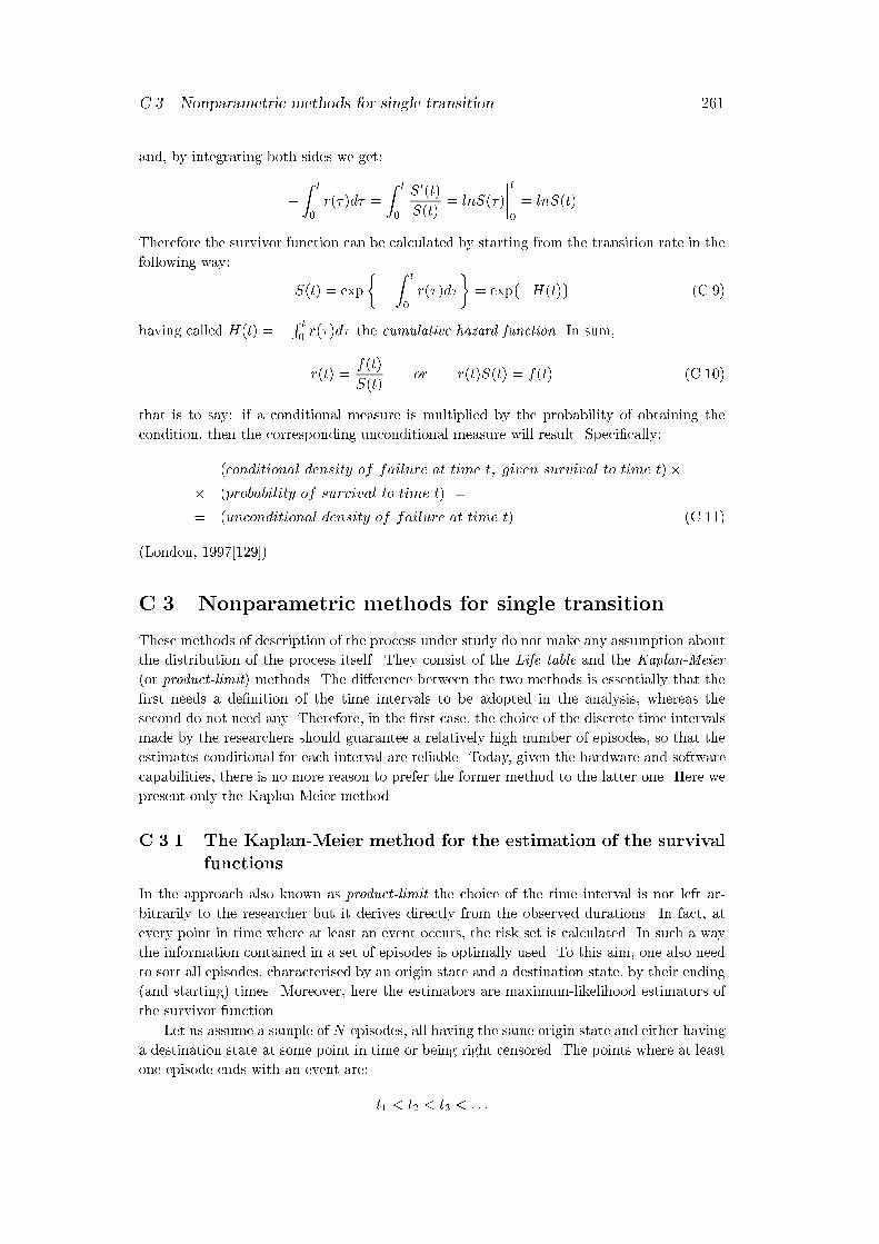
C.3. Nonparametric methods for single transition 261
and, by integrating both sides we get:
�
Z t
0
r(�)d� =
Z t
0
S0(t)
S(t)= lnS(�)
����t
0
= lnS(t)
Therefore the survivor function can be calculated by starting from the transition rate in the
following way:
S(t) = exp
��
Z t
0
r(�)d�
�= expf�H(t)g (C.9)
having called H(t) = �R t0r(�)d� the cumulative hazard function. In sum,
r(t) =f(t)
S(t)or r(t)S(t) = f(t) (C.10)
that is to say: if a conditional measure is multiplied by the probability of obtaining the
condition, then the corresponding unconditional measure will result. Speci�cally:
(conditional density of failure at time t; given survival to time t)�
� (probability of survival to time t) =
= (unconditional density of failure at time t) (C.11)
(London, 1997[129]).
C.3 Nonparametric methods for single transition
These methods of description of the process under study do not make any assumption about
the distribution of the process itself. They consist of the Life table and the Kaplan-Meier
(or product-limit) methods. The di�erence between the two methods is essentially that the
�rst needs a de�nition of the time intervals to be adopted in the analysis, whereas the
second do not need any. Therefore, in the �rst case, the choice of the discrete time intervals
made by the researchers should guarantee a relatively high number of episodes, so that the
estimates conditional for each interval are reliable. Today, given the hardware and software
capabilities, there is no more reason to prefer the former method to the latter one. Here we
present only the Kaplan-Meier method.
C.3.1 The Kaplan-Meier method for the estimation of the survival
functions
In the approach also known as product-limit the choice of the time interval is not left ar-
bitrarily to the researcher but it derives directly from the observed durations. In fact, at
every point in time where at least an event occurs, the risk set is calculated. In such a way
the information contained in a set of episodes is optimally used. To this aim, one also need
to sort all episodes, characterised by an origin state and a destination state, by their ending
(and starting) times. Moreover, here the estimators are maximum-likelihood estimators of
the survivor function.
Let us assume a sample of N episodes, all having the same origin state and either having
a destination state at some point in time or being right censored. The points where at least
one episode ends with an event are:
t1 < t2 < t3 < : : :
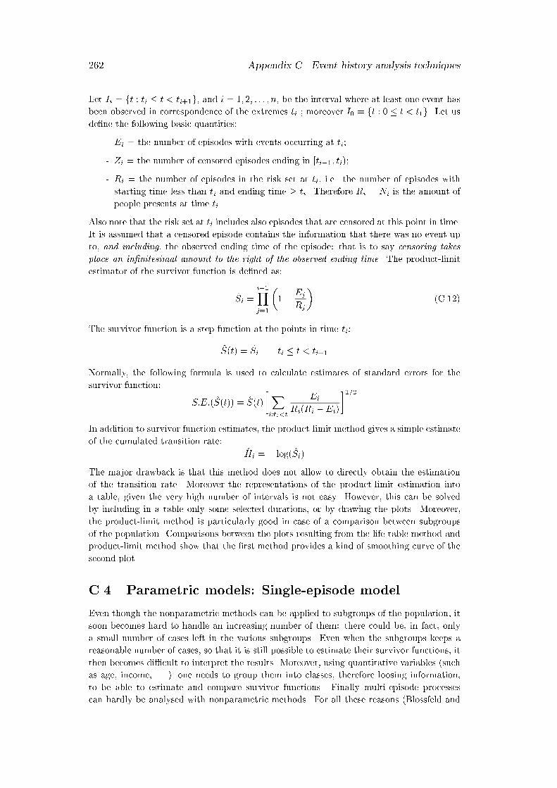
262 Appendix C. Event history analysis techniques
Let Ii = ft : ti � t < ti+1g, and i = 1; 2; : : : ; n, be the interval where at least one event has
been observed in correspondence of the extremes ti ; moreover I0 = ft : 0 � t < t1g. Let us
de�ne the following basic quantities:
- Ei = the number of episodes with events occurring at ti;
- Zi = the number of censored episodes ending in [ti�1; ti);
- Ri = the number of episodes in the risk set at ti, i.e. the number of episodes with
starting time less than ti and ending time � ti. Therefore Ri = Ni is the amount of
people presents at time ti.
Also note that the risk set at ti includes also episodes that are censored at this point in time.
It is assumed that a censored episode contains the information that there was no event up
to, and including, the observed ending time of the episode: that is to say censoring takes
place an in�nitesimal amount to the right of the observed ending time. The product-limit
estimator of the survivor function is de�ned as:
Si =
i�1Yj=1
�1�
Ej
Rj
�(C.12)
The survivor function is a step function at the points in time ti:
S(t) = Si ti � t < ti+1
Normally, the following formula is used to calculate estimates of standard errors for the
survivor function:
S:E:(S(t)) = S(t)
� Xi:ti<t
Ei
Ri(Ri �Ei)
�1=2
In addition to survivor function estimates, the product-limit method gives a simple estimate
of the cumulated transition rate:
Hi = � log(Si)
The major drawback is that this method does not allow to directly obtain the estimation
of the transition rate. Moreover the representations of the product-limit estimation into
a table, given the very high number of intervals is not easy. However, this can be solved
by including in a table only some selected durations, or by drawing the plots. Moreover,
the product-limit method is particularly good in case of a comparison between subgroups
of the population. Comparisons between the plots resulting from the life table method and
product-limit method show that the �rst method provides a kind of smoothing curve of the
second plot.
C.4 Parametric models: Single-episode model
Even though the nonparametric methods can be applied to subgroups of the population, it
soon becomes hard to handle an increasing number of them: there could be, in fact, only
a small number of cases left in the various subgroups. Even when the subgroups keeps a
reasonable number of cases, so that it is still possible to estimate their survivor functions, it
then becomes di�cult to interpret the results. Moreover, using quantitative variables (such
as age, income, . . . ) one needs to group them into classes, therefore loosing information,
to be able to estimate and compare survivor functions. Finally multi-episode processes
can hardly be analysed with nonparametric methods. For all these reasons (Blossfeld and
C.4. Parametric models: Single-episode model 263
Rohwer, 1995[24]) over the last 20 years, event history analysis has been mainly based
on parametric transition rate models, using nonparametric methods as descriptive tools.
Transition rate models o�er also the possibility to include in the model the dependence on
a set of covariates.
C.4.1 Maximum Likelihood Estimates
The general feature of the models will be explained in two steps: �rst we look at the case of
single transition where there is a single random variable T and then we look at the case of
multiple destinations with a two-dimensional random variables (this case will be exploited in
the next chapter, but it is useful to introduce the concept right now) (Blossfeld and Rohwer,
1995[24], Rohwer and P�otter, 1998[150]).
Let us start with the simplest case. To derive the model, one has to assume a known
parametric distribution for the duration variable T , whose parameters are a; b; c; : : : The
cumulative distribution function is:
F (t; a; b; c; : : :) =
Z t
0
f(� ; a; b; c; : : :)d�
the survivor function is:
S(t; a; b; c; : : :) = 1� F (t; a; b; c; : : :)
and the transition rate is given by:
r(t; a; b; c; : : :) =f(t; a; b; c; : : :)
S(t; a; b; c; : : :)
In the case of single transition we want to study the transition rate from origin state j 2 O
to destination state in ,Dj , which represents the set of all possible destination states for
episodes having an origin state j. Let
- Nj the set of all episodes with origin state j,
- Zj the set of all censored episodes having an origin state j,
- Ejk the set of all episodes with origin state j and destination state k that have an
event (j 6= k).
To simplify notation let us omit the dependence on the set of parameters. In the case of a
single transition (j; k) the likelihood can be written as:
Ljk =Yi2Ejk
f(ti)Yi2Zj
S(ti) =Yi2Ejk
r(ti)Yi2Nj
S(ti) (C.13)
As the usual notation: f(t) is the density function and S(t) is the survivor function for the
single transition (j; k). Therefore if the episode has one event at ti, its contribution to the
likelihood is given by the density function, calculated at the ending time ti; if the episode
is censored, its contribution to the likelihood is given by the survivor function evaluated
at the ending time ti, but possibly depends on covariates changing their values during the
episode. Thus the likelihood function can be expressed by using only the transition rate and
the survivor function. Also covariates, that may change their values during the episode can
be included in the model.
In case of transitions to multiple destinations, transition rates describe the movements
from an origin state j 2 O to two or more destination states k 2 Dj , which represent the set

264 Appendix C. Event history analysis techniques
of all possible destination states for episodes having an origin state j. In this case there is a
two-dimensional random variable (Tj ; Dj), with Tj the duration in the origin state and Dj
the destination state after leaving the origin state. Generalising the concept of transition
rate to this case we de�ne the transition-speci�c rates by:
rjk(t) = lim�t!0
P (t � T < t+�t;Dj = kjT � t)
�t= lim
�t!0
P (t � T < t+�t;Dj = k)
�t
1
P (T � t)(C.14)
Thus, assuming that all the transition rates rjk have the same mathematical form, there is
only the need to generalise the single-transition case to a situation with alternative desti-
nation states. In particular, we can de�ne the transition speci�c rate as a single-transition
case and provide the possibility for transition-speci�c parameters:
rjk(t; ajk ; bjk; cjk ; : : :) = r(t; ajk ; bjk; cjk ; : : :)
where the parameters are transition-speci�c and r(t; : : :) is taken from the single-transition
case. The survivor functions Sj(t) for the duration in the given origin state j 2 O can be
derived from the pseudo-survivor functions speci�c for each transition
~Sjk(t) = exp
��
Z t
0
rjk(�)d�
�:
Given that the transition rate has the same mathematical form for each kind of transition
as the corresponding single-transition case, we have
~Sj(t) =Yk2Dj
~Sjk(t) (C.15)
Model estimations generally assumes that the individuals episodes are statistically inde-
pendent and this might not be true especially in the case of multiple episodes, when each
individual can contribute to more than one episode. But this requirement is conditional on
covariates, and can be often met by using covariates to capture information about the past
history of the individual episodes. The likelihood can be written as:
Lj =Yk2Dj
Yi2Ejk
~fjk(ti)Yi2Zj
Sj(ti) =Yk2Dj
Yi2Ejk
rjk(ti)Yi2Nj
Sj(ti) (C.16)
Lj =Yk2Dj
Yi2Ejk
rjk(ti)Yk2Dj
Yi2Nj
~Sjk(ti) (C.17)
where, in the second passage, Sj(ti) has been substituted according to equation (C.15). By
rearranging we obtain the likelihood function in the case of multiple destinations from the
origin state j.
Lj =Yk2Dj
� Yi2Ejk
rjk(ti)Yi2Nj
~Sjk(ti)
�(C.18)
Lastly, the third step is to account for more than a single origin state. In this case, it is
necessary to multiply the (C.18) by the product over all the possible origin states j:
L =Yj2O
Lj =Yj2O
Yk2Dj
Yi2Ejk
rjk(ti)Yi2Nj
~Sjk(ti) (C.19)
The last equation (C.19) represents the most general form of the likelihood: in the case of
a single origin state and a single destination state it becomes (C.13) and in the multiple
destinations case it becomes (C.18). The total log-likelihood function is :
` =Xj2O
Xk2Dj
Xi2Ejk
logfrjk(ti)g+Xi2Nj
logf ~Sjk(ti)g (C.20)
C.4. Parametric models: Single-episode model 265
The fact that the total likelihood (C.19) can result from the product of transition-speci�c
factors implies that, in the case of several transitions, a model for each transition can be
estimated separately1. To estimate the single transition (j; k), the episode with starting state
j will be taken into account; then those ending in the destination state k are considered as
having an event, and all other events are regarded as censored. Moreover, the factorisation
of the total likelihood allows also for the choice of di�erent speci�cation of the rates for
di�erent transitions.
C.4.2 The piecewise constant exponential model
This model represents a generalisation of the exponential model (which we do not describe
here), and provide a very useful tool of description of the transition rate. The basic idea
is to split the time axis into periods and assume that transition rates are constant in each
period but may vary across them
In particular, if we specify a set of covariates we have two di�erent options. On one
hand we can assume that only a baseline rate, given by period-speci�c constants can vary
across time-periods but the covariates have the same (proportional) e�ects in each period.
On the other hand, we could allow for period-speci�c e�ects of covariates also.
In the �rst case, when the e�ects of the covariates do not change across time periods,
let us imagine dividing the time-axis into m time periods, then the distribution of durations
has m parameters2:
0 = �1 < �2 < �3 < : : : < �m =1
according to which we also have:
Il = ftj�l � t < �l+1g l = 1; 2; : : : ;m:
Therefore, the transition rate from origin state j to destination state k is given by:
rjk(t) = expf��(jk)l +A(jk)�(jk)g if t 2 Il:
For each transition (j; k), ��(jk)l is a constant coe�cient associated with the lth time period,
therefore it represents the time varying components of the rate. A(jk) is a row vector of
covariates and �(jk) is an associated vector of coe�cients assumed not to vary across time
periods. The model must not contain a separate constant (it can be included in constant
part of the component). If we do not specify any covariate (that is we do not include any
A(jk) component), then the model estimate only the parameters for the baseline rate (given
by exp ��(jk)).
In the second case, we allow the e�ect of the covariates to change across time. Now,
case the transition rate relative to transition (jk) becomes:
rjk(t) = expf��(jk)l +A(jk)�
(jk)l g if t 2 Il:
1Of course, this is only possible if there are no constraints on parameters across di�erent transi-
tions. To provide for this possibility is the main reason for using the likelihood (Rohwer and P�otter,
1998[150]).2The choice of an appropriate number of intervals is subject to speci�c considerations. Evidently,
the more the intervals, the best the approximation of the unknown baseline rate, but this implies a
large number of coe�cients to be estimated. On the other hand, a small number of intervals is less
problematic as concern the estimations, but provides a rough approximation of the baseline rate.
Therefore, it is wise to search for a compromise between the two alternatives. Another obvious
requirements is building intervals with ending times for some episodes: that is to say, intervals
should contain events.
266 Appendix C. Event history analysis techniques
In fact, we now have �(jk)l which depends on time as ��
(jk)l and is speci�c for the lth interval.
As can be noted this case represents a generalisation of the previous which can in fact be
obtained by constraining to be equal the parameters �(jk)l values across time periods.
C.5 Semi-Parametric transition rate models: Propor-
tional Hazards Model
Up to now our aim was to describe the duration of an episode (using a nonparametric
analysis) or to model the transition rate of an episode by allowing for its dependence on
time (and on a set of covariates as well). One of the problem in social sciences is that theories
only rarely o�er the possibility to introduce a speci�c parametric model for the phenomenon
under study. We shall therefore very carefully choose and apply a speci�c model as it need
to know `how' the hazard rate depends on time (its shape). From this point of view, also
the checks on the goodness-of-�t which may provide some hints on discerning which class of
model might be preferable, do not give us the certainty of supporting a speci�c parametric
model. The adequacy of parametric models could be evaluated by heuristic models (graphical
comparisons, or comparison with nonparametric functions)(Blossfeld and Rohwer, 1995[24]).
An alternative procedure could be to specify only the functional form for the in uence of
covariates but to leave the shape of the transition rate as unspeci�ed as possible.
This model is characterised by a robustness given that it can estimate the coe�cients
even though the baseline hazard is unspeci�ed. Moreover, the exponential factor, in the
second right hand of the equation, ensures that the �tted model will give non-negative
hazards.
The proportional hazards model, also known asCox regression model, has been introduced
in the medical research to evaluate the e�ect of covariates (age, blood pressure, life styles,
etc.) on the duration of an episode (particularly on the risk of death). Its aim is therefore to
evaluate which combination of potential explanatory variables a�ect the form of the hazard
function (Collett, 1997[55]). It may be written as
r(t) = r0(t) exp(�1X1 + �2X2(t) + : : :) (C.21)
so that the transition rate r(t) can be written as the product of an unspeci�ed baseline
rate r0(t) and a second term specifying the possible in uence of a set of covariates (they
might also depend on time). The � coe�cients express the e�ect of the covariates as in the
parametric models. We talk about proportional hazard model because the increase of a unit
of the generic covariate Xi produces a proportional shift in the transition rate but cannot
change its shape: the rate will be equal to the product between the baseline rate and the
factor exp(�i).
It should be stressed that the Cox model is sensible only when a set of covariates are
introduced: in fact it does not even produce the value of an intercept (all constant e�ects
are included in the baseline). The use of the Cox model is particularly appropriate in the
following situations: for instance when the researcher has no clear idea about the shape of
time dependence, or when the theory does not support any speci�c model, or when the trend
of the process is known but it is not known the distribution of the uctuations, or, lastly,
when the interest is on the evaluation of the magnitude and the direction of the e�ects of
the covariates, controlling for time-dependence (Blossefeld and Rohwer, 1995[24]).
Two basic assumptions are involved in proportional hazards models (Namboodiri and
Suchindran, 1987[140]):

C.5. Semi-Parametric transition rate models: Proportional Hazards Model 267
1) all individuals with a given con�guration of values for the covariates x1; x2; : : : have
identical hazards functions,
2) the hazards functions of any two individuals di�ering in the con�guration of values of
the covariates have parallel age (time) patterns (proportionality assumption).
C.5.1 Partial Likelihood Estimation
Let us imagine that among n individuals we observe a total number of events equals to r
and a total number of censoring equals to n � r. The basis of the argument used in the
construction of a likelihood function for the proportional hazards model is that intervals
between successive events times convey no information about the e�ect of explanatory vari-
ables on the transition rate (in particular we refer here to Collett, 1997[55]). The reason is
that, as the hazard has an arbitrary form, it could also be r0(t) = 0 and hence r(t) = 0 in
those time intervals in which there are no events. As a results, these intervals do not give
any information about the values of the � parameters. Now, we indicate as follows the times
where one event is observed:
t(1); t(2); : : : ; t(r)
and the vector of the covariate for the individual experiencing one event at t(j) is X(j) =
[X1(j) X2(j) : : :Xc(j)]. Therefore:
P [individual with variables X(j) has an event at t(j)jthere is anevent in t(j)] =
=P [individual with variablesX(j) has an event at t(j)]
P [there is an event in t(j)](C.22)
The numerator of the above expression is simply the hazard of the transition in t(j) for those
who have the speci�ed vector of covariates. The denominator is the sum of the hazards of
the event at time t(j) over all individuals who are at risk of events at this time. This is the
sum of the values rl(t(j)) over those indexes by l in the risk set at time t(j), R(t(j)):
Xi2R(t(j))
rl(t(j)) =X
i2R(t(j))
r0(t(j)) exp(�1X1(i) + �2X2(i) + : : :)
Therefore the previous expression becomes:
exp(�1X1(i) + �2X2(i) + : : :)Pi2R(t(j))
exp(�1X1(i) + �2X2(i) + : : :)
This is the contribution to the partial likelihood of the ith individual. Finally, taking the
product of these conditional probabilities over the r times where an event occurs gives the
partial likelihood function:
Lp(�1; �2; : : :) =
rYj=1
exp(�1X1(i) + �2X2(i) + : : :)Pi2R(t(j))
exp(�1X1(i) + �2X2(i) + : : :)(C.23)
The likelihood obtained is not a true likelihood, since it does not make direct use of the actual
censored and uncensored survival times, and for this reason it is called partial likelihood
function.
The major problem of the proportional hazards model for survival data is that it as-
sumes that tied survival times (events occurring at the same time) are not possible. In
fact it assumes that in each time point only an event occurs. In order to accommodate
tied observations, the likelihood function in equation C.23 has to be modi�ed in some way.
268 Appendix C. Event history analysis techniques
Kalb eisch and Prentice (1980[110]) provides a likelihood function which takes into account
the problem of the tied observations, but its computation is very time consuming, especially
when there are a lot of tied observations. We can then recur to one of the approximation to
the likelihood function, as, for instance, the one suggested by Breslow (1974) according to
which, if in time t(j) we have dj events belonging to the set Dj , the partial likelihood can
be approximated by:
Pj2Dj
exp(�1X1(i) + �2X2(i) + : : :)Pj2R(t(i))
exp(�1X1(i) + �2X2(i) + : : :)=
rYj=1
exp(�1X1(i) + �2X2(i) + : : :)Pj2R(t(i))
exp(�1X1(i) + �2X2(i) + : : :)
(C.24)
This approximation is an adequate approximation when the number of tied observations at
any one event time is not too large.
C.5.2 Interpretation of the parameters
The coe�cient of the explanatory variables in the model can be interpreted as logarithms
of the ratio of the hazard of the event to the baseline hazard. The interpretation of the
parameters corresponds to di�erent types of term in the proportional hazard model. For
instance, if we have a model with variate, a single continuous variable X which assumes the
value xi on the ith individual, the hazard function will be given by:
ri(t) = exp(�xi)r0(t)
where the coe�cient of xi can be interpreted as the logarithm of a hazard ratio. Now consider
two individuals for which the value x and x + 1 of the X variable have been recorded, the
ratio of their hazards is given by:
exp(�(x + 1))
exp(�x)= exp(�)
so that � in the �tted proportional hazards model is the estimated change in the logarithm
of the hazard ratio when the value of X is increased by one unit.
In the same way, when the value of the variable X is increased by c units, the estimated
change in the log-hazard ratio is c�, and the corresponding estimate of the hazard ratio is
exp(c�). The standard error of the estimated log-hazard ratio will be cs:e:(�) form which
con�dence intervals for the true hazard ratio can be derived. As Collett highlights, the above
argument shows that when a continuous variable X is included in a proportional hazards
model, the hazard ratio when the value of X is changed by c does not depend on the actual
value of X. For example, if X refers to the age of an individual, the hazard ratio for an
individual aged 70, relative to one aged 65, would be the same as that for an individual aged
20, relative to one aged 15. This feature is a direct result of �tting X as a linear term in the
proportional hazards model. If there is doubt about the assumption of linearity, a factor
whose levels correspond to di�erent sets of values of X can be �tted. Moreover the linearity
assumption can be checked.
When we have individuals divided into m groups according to the categories of a cate-
gorical variable, the groups can be indexed by the levels of a factor. The hazard function
for an individual in the jth group, j = 1; 2; : : : ;m is given by:
rj(t) = exp( j)r0(t);
where j is the e�ect due to the jth level of the factor and r0(t) is the baseline hazard
function. This model is overparametrized and so we take 1 = 0. The baseline hazard
C.6. Comparing parametric models 269
function then corresponds to the hazard of death at time t for an individual in the �rst
group. The ratio of the hazards at time t for an individual in the jth groups, relative to an
individual in the �rst group is then exp( j). Consequently, the parameter j is the logarithm
of this relative hazard that is :
j = log rj(t)=r0(t):
A model which contains the terms j , j = 1; 2; : : : ;m with the 1 = 0 can be �tted by
de�ning m� 1 indicator variables X2;X3; : : : ;Xm as shown in....
C.5.3 The proportionality assumption
A basic feature of the Cox model is that transition rates for di�erent values of covariates are
proportional. If, for instance, we have two groups whose transition rates are r(t) and r0(t)
and whose values of the ith covariate are xi and x0i respectively then
r(t) = expf(xi � x0i)�igr0(t)
which expresses the proportionality assumption. To check the proportionality assumption
one could adopt the graphical method.
S(t) = exp(�
Z t
0
r(�)d�) = expf(xi � x0i)�igr0(t)
If, for some covariates, the proportionality assumption is not acceptable it is sometimes
sensible to estimate a strati�ed model. This is only possible for categorical covariates where
every groups constitutes a strata. In this way we can obtain a baseline function for each
di�erent group.
C.6 Comparing parametric models
To select the best model among a set of alternative nested ones (characterised by an in-
cremental number of parameters) one uses the likelihood ratio test (Yamaguchi, 1991[191]).
Let us imagine to have a model with k parameters and loglikelihood lk to be compared to
another more general one with k+h parameters and whose loglikelihood is denoted by lk+h.
Two models ar nested if and only if one model is obtained by adding some parameter(s)
to the other model. The likelihood-ratio test for comparing nested models, test the null
hypothesis that expected values from the models are identical except for di�erences due to
random variation.
�2 logLk
Lk+h= �2(`k � `k+h) � �2h (C.25)
It follows that, if the di�erence in chi-square between two nested models is signi�cant for a
given di�erence in the degrees of freedom, we should reject the null hypothesis and conclude
that the model that has more parameters improves the �t of the model with fewer parame-
ters. On the other hand, if the di�erence in chi-square is insigni�cant, we cannot reject the
null hypothesis. Then we should accept the model with fewer parameters as having a more
parsimonious �t with the data than the model with more parameters.
In case of nonnested models, a di�erent selection procedure has to be followed. Therefore
models with di�erent sets of covariates can be compared, for instance, by the Akaike's
Information Criterion (AIC) or by the Bayesian Information Criterion (BIC), also known
as the Schwartz's method. The �rst procedure gives:
AIC = �2`+ 3pk (C.26)
270 Appendix C. Event history analysis techniques
where pk is the number of unknown parameters and the criterion is based on the choice
of the lowest AIC. The BIC procedure, which approximates the Bayes factor (Kass and
Raftery, 1995[116]) is de�ned as:
BIC = ��2k0 + pk logn (C.27)
where �2k0 is the well-known likelihood ratio of the used model compared to the model
without independent variables, pk is the number of unknown parameters and n is the number
of events. The choice will fall on the model with lowest BIC.

Appendix D
Notes on chapter 4
271
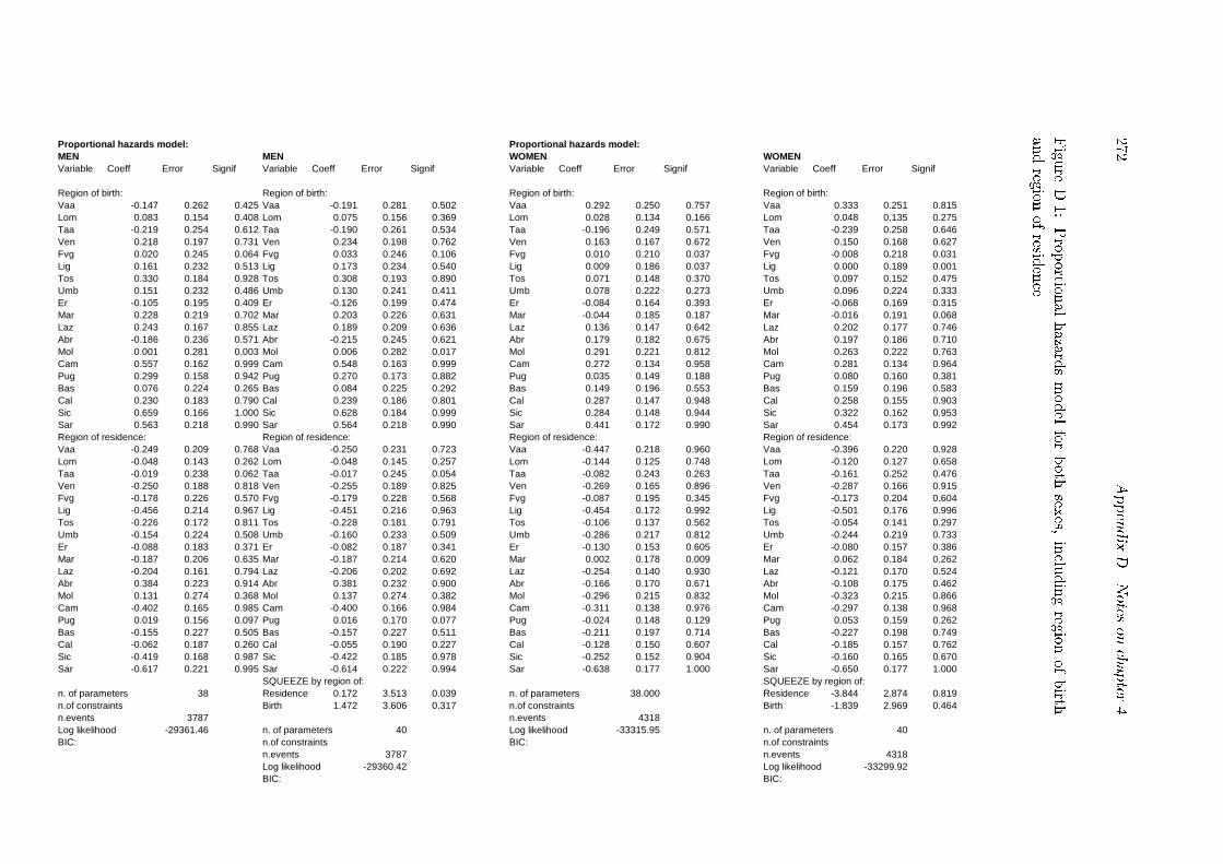
272
Appendix
D.Notes
onchapter
4
Figure
D.1:Proportio
nalhazardsmodel
forboth
sexes,
inclu
dingreg
ionofbirth
andreg
ionofresid
ence
Proportional hazards model: Proportional hazards model:MEN MEN WOMEN WOMENVariable Coeff Error Signif Variable Coeff Error Signif Variable Coeff Error Signif Variable Coeff Error Signif
Region of birth: Region of birth: Region of birth: Region of birth:Vaa -0.147 0.262 0.425 Vaa -0.191 0.281 0.502 Vaa 0.292 0.250 0.757 Vaa 0.333 0.251 0.815Lom 0.083 0.154 0.408 Lom 0.075 0.156 0.369 Lom 0.028 0.134 0.166 Lom 0.048 0.135 0.275Taa -0.219 0.254 0.612 Taa -0.190 0.261 0.534 Taa -0.196 0.249 0.571 Taa -0.239 0.258 0.646Ven 0.218 0.197 0.731 Ven 0.234 0.198 0.762 Ven 0.163 0.167 0.672 Ven 0.150 0.168 0.627Fvg 0.020 0.245 0.064 Fvg 0.033 0.246 0.106 Fvg 0.010 0.210 0.037 Fvg -0.008 0.218 0.031Lig 0.161 0.232 0.513 Lig 0.173 0.234 0.540 Lig 0.009 0.186 0.037 Lig 0.000 0.189 0.001Tos 0.330 0.184 0.928 Tos 0.308 0.193 0.890 Tos 0.071 0.148 0.370 Tos 0.097 0.152 0.475Umb 0.151 0.232 0.486 Umb 0.130 0.241 0.411 Umb 0.078 0.222 0.273 Umb 0.096 0.224 0.333Er -0.105 0.195 0.409 Er -0.126 0.199 0.474 Er -0.084 0.164 0.393 Er -0.068 0.169 0.315Mar 0.228 0.219 0.702 Mar 0.203 0.226 0.631 Mar -0.044 0.185 0.187 Mar -0.016 0.191 0.068Laz 0.243 0.167 0.855 Laz 0.189 0.209 0.636 Laz 0.136 0.147 0.642 Laz 0.202 0.177 0.746Abr -0.186 0.236 0.571 Abr -0.215 0.245 0.621 Abr 0.179 0.182 0.675 Abr 0.197 0.186 0.710Mol 0.001 0.281 0.003 Mol 0.006 0.282 0.017 Mol 0.291 0.221 0.812 Mol 0.263 0.222 0.763Cam 0.557 0.162 0.999 Cam 0.548 0.163 0.999 Cam 0.272 0.134 0.958 Cam 0.281 0.134 0.964Pug 0.299 0.158 0.942 Pug 0.270 0.173 0.882 Pug 0.035 0.149 0.188 Pug 0.080 0.160 0.381Bas 0.076 0.224 0.265 Bas 0.084 0.225 0.292 Bas 0.149 0.196 0.553 Bas 0.159 0.196 0.583Cal 0.230 0.183 0.790 Cal 0.239 0.186 0.801 Cal 0.287 0.147 0.948 Cal 0.258 0.155 0.903Sic 0.659 0.166 1.000 Sic 0.628 0.184 0.999 Sic 0.284 0.148 0.944 Sic 0.322 0.162 0.953Sar 0.563 0.218 0.990 Sar 0.564 0.218 0.990 Sar 0.441 0.172 0.990 Sar 0.454 0.173 0.992Region of residence: Region of residence: Region of residence: Region of residence:Vaa -0.249 0.209 0.768 Vaa -0.250 0.231 0.723 Vaa -0.447 0.218 0.960 Vaa -0.396 0.220 0.928Lom -0.048 0.143 0.262 Lom -0.048 0.145 0.257 Lom -0.144 0.125 0.748 Lom -0.120 0.127 0.658Taa -0.019 0.238 0.062 Taa -0.017 0.245 0.054 Taa -0.082 0.243 0.263 Taa -0.161 0.252 0.476Ven -0.250 0.188 0.818 Ven -0.255 0.189 0.825 Ven -0.269 0.165 0.896 Ven -0.287 0.166 0.915Fvg -0.178 0.226 0.570 Fvg -0.179 0.228 0.568 Fvg -0.087 0.195 0.345 Fvg -0.173 0.204 0.604Lig -0.456 0.214 0.967 Lig -0.451 0.216 0.963 Lig -0.454 0.172 0.992 Lig -0.501 0.176 0.996Tos -0.226 0.172 0.811 Tos -0.228 0.181 0.791 Tos -0.106 0.137 0.562 Tos -0.054 0.141 0.297Umb -0.154 0.224 0.508 Umb -0.160 0.233 0.509 Umb -0.286 0.217 0.812 Umb -0.244 0.219 0.733Er -0.088 0.183 0.371 Er -0.082 0.187 0.341 Er -0.130 0.153 0.605 Er -0.080 0.157 0.386Mar -0.187 0.206 0.635 Mar -0.187 0.214 0.620 Mar 0.002 0.178 0.009 Mar 0.062 0.184 0.262Laz -0.204 0.161 0.794 Laz -0.206 0.202 0.692 Laz -0.254 0.140 0.930 Laz -0.121 0.170 0.524Abr 0.384 0.223 0.914 Abr 0.381 0.232 0.900 Abr -0.166 0.170 0.671 Abr -0.108 0.175 0.462Mol 0.131 0.274 0.368 Mol 0.137 0.274 0.382 Mol -0.296 0.215 0.832 Mol -0.323 0.215 0.866Cam -0.402 0.165 0.985 Cam -0.400 0.166 0.984 Cam -0.311 0.138 0.976 Cam -0.297 0.138 0.968Pug 0.019 0.156 0.097 Pug 0.016 0.170 0.077 Pug -0.024 0.148 0.129 Pug 0.053 0.159 0.262Bas -0.155 0.227 0.505 Bas -0.157 0.227 0.511 Bas -0.211 0.197 0.714 Bas -0.227 0.198 0.749Cal -0.062 0.187 0.260 Cal -0.055 0.190 0.227 Cal -0.128 0.150 0.607 Cal -0.185 0.157 0.762Sic -0.419 0.168 0.987 Sic -0.422 0.185 0.978 Sic -0.252 0.152 0.904 Sic -0.160 0.165 0.670Sar -0.617 0.221 0.995 Sar -0.614 0.222 0.994 Sar -0.638 0.177 1.000 Sar -0.650 0.177 1.000
SQUEEZE by region of: SQUEEZE by region of:n. of parameters 38 Residence 0.172 3.513 0.039 n. of parameters 38.000 Residence -3.844 2.874 0.819n.of constraints Birth 1.472 3.606 0.317 n.of constraints Birth -1.839 2.969 0.464n.events 3787 n.events 4318Log likelihood -29361.46 n. of parameters 40 Log likelihood -33315.95 n. of parameters 40BIC: n.of constraints BIC: n.of constraints
n.events 3787 n.events 4318Log likelihood -29360.42 Log likelihood -33299.92BIC: BIC:
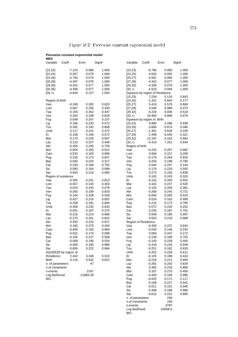
273
Figure D.2: Piecewise constant exponential model
Piecewise constant exponential model:MENVariable Coeff Error Signif Variable Coeff Error Signif
[15,22) -7.124 0.086 1.000 [15,23) -6.786 0.080 1.000[22,24) -5.357 0.079 1.000 [23,25) -4.932 0.083 1.000[24,26) -4.750 0.075 1.000 [25,27) -4.561 0.080 1.000[26,28) -4.497 0.075 1.000 [27,29) -4.342 0.077 1.000[28,30) -4.331 0.077 1.000 [29,32) -4.338 0.076 1.000[30,35) -4.398 0.077 1.000 [32,+) -4.510 0.094 1.000[35,+) -4.844 0.127 1.000 Squeeze by region of Residence
[15,23) 7.234 5.116 0.843Region of birth [23,25) -1.251 5.604 0.177Vaa -0.249 0.282 0.623 [25,27) 5.419 5.579 0.669Lom 0.067 0.156 0.330 [27,29) 0.546 5.988 0.073Taa -0.155 0.262 0.447 [29,32) -4.226 6.006 0.518Ven 0.264 0.198 0.818 [32,+) 15.955 6.889 0.979Fvg 0.049 0.247 0.157 Squeeze by region of BirthLig 0.186 0.233 0.573 [15,23) 9.880 5.286 0.938Tos 0.282 0.192 0.858 [23,25) 0.685 5.674 0.096Umb 0.117 0.241 0.372 [25,27) -1.391 5.628 0.195Er -0.158 0.199 0.572 [27,29) 2.499 6.045 0.321Mar 0.174 0.226 0.557 [29,32) 12.197 6.103 0.954Laz 0.123 0.207 0.448 [32,+) -5.414 7.261 0.544Abr -0.256 0.245 0.705 Region of birthMol 0.004 0.283 0.012 Vaa -0.232 0.287 0.582Cam 0.533 0.163 0.999 Lom 0.060 0.157 0.299Pug 0.235 0.173 0.827 Taa -0.179 0.264 0.503Bas 0.092 0.224 0.317 Ven 0.254 0.198 0.799Cal 0.234 0.186 0.792 Fvg 0.045 0.247 0.144Sic 0.590 0.184 0.999 Lig 0.176 0.233 0.550Sar 0.563 0.218 0.990 Tos 0.270 0.193 0.838Region of residence Umb 0.102 0.243 0.325Vaa -0.305 0.231 0.813 Er -0.152 0.200 0.553Lom -0.057 0.145 0.303 Mar 0.162 0.227 0.525Taa 0.024 0.245 0.078 Laz 0.104 0.209 0.381Ven -0.260 0.189 0.833 Abr -0.266 0.245 0.721Fvg -0.164 0.228 0.528 Mol -0.004 0.283 0.010Lig -0.427 0.216 0.952 Cam 0.524 0.163 0.999Tos -0.258 0.181 0.846 Pug 0.215 0.173 0.785Umb -0.209 0.232 0.633 Bas 0.072 0.225 0.252Er -0.091 0.187 0.375 Cal 0.235 0.187 0.791Mar -0.216 0.214 0.688 Sic 0.549 0.185 0.997Laz -0.270 0.201 0.822 Sar 0.553 0.218 0.989Abr 0.352 0.232 0.871 Region of ResidenceMol 0.165 0.275 0.450 Vaa -0.335 0.237 0.843Cam -0.400 0.165 0.984 Lom -0.043 0.146 0.232Pug -0.021 0.170 0.099 Taa 0.054 0.247 0.172Bas -0.156 0.227 0.508 Ven -0.238 0.189 0.792Cal -0.008 0.190 0.034 Fvg -0.140 0.228 0.460Sic -0.465 0.185 0.988 Lig -0.418 0.216 0.948Sar -0.605 0.222 0.994 Tos -0.251 0.182 0.833SQUEEZE by region of: Umb -0.202 0.234 0.611Residence 2.442 3.438 0.523 Er -0.105 0.188 0.424Birth 3.116 3.532 0.622 Mar -0.218 0.214 0.690n. of parameters 47 Laz -0.281 0.203 0.834n.of constraints Abr 0.362 0.233 0.880n.events 3787 Mol 0.167 0.275 0.456Log likelihood -21883.28 Cam -0.405 0.166 0.985BIC: Pug -0.025 0.171 0.117
Bas -0.168 0.227 0.541Cal -0.011 0.191 0.045Sic -0.458 0.186 0.986Sar -0.615 0.222 0.995n. of parameters 246n.of constraints 190n.events 3787Log likelihood -22008.6BIC:
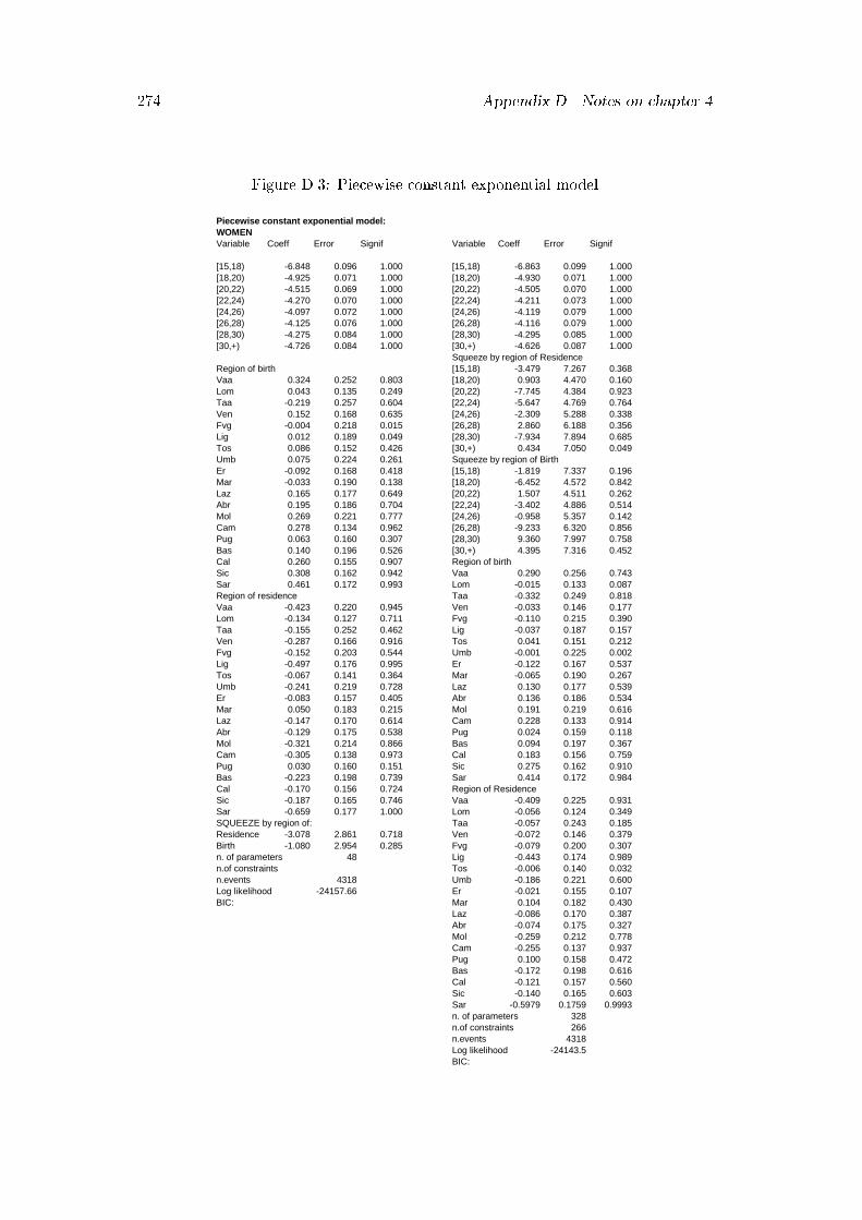
274 Appendix D. Notes on chapter 4
Figure D.3: Piecewise constant exponential model
Piecewise constant exponential model:WOMENVariable Coeff Error Signif Variable Coeff Error Signif
[15,18) -6.848 0.096 1.000 [15,18) -6.863 0.099 1.000[18,20) -4.925 0.071 1.000 [18,20) -4.930 0.071 1.000[20,22) -4.515 0.069 1.000 [20,22) -4.505 0.070 1.000[22,24) -4.270 0.070 1.000 [22,24) -4.211 0.073 1.000[24,26) -4.097 0.072 1.000 [24,26) -4.119 0.079 1.000[26,28) -4.125 0.076 1.000 [26,28) -4.116 0.079 1.000[28,30) -4.275 0.084 1.000 [28,30) -4.295 0.085 1.000[30,+) -4.726 0.084 1.000 [30,+) -4.626 0.087 1.000
Squeeze by region of ResidenceRegion of birth [15,18) -3.479 7.267 0.368Vaa 0.324 0.252 0.803 [18,20) 0.903 4.470 0.160Lom 0.043 0.135 0.249 [20,22) -7.745 4.384 0.923Taa -0.219 0.257 0.604 [22,24) -5.647 4.769 0.764Ven 0.152 0.168 0.635 [24,26) -2.309 5.288 0.338Fvg -0.004 0.218 0.015 [26,28) 2.860 6.188 0.356Lig 0.012 0.189 0.049 [28,30) -7.934 7.894 0.685Tos 0.086 0.152 0.426 [30,+) 0.434 7.050 0.049Umb 0.075 0.224 0.261 Squeeze by region of BirthEr -0.092 0.168 0.418 [15,18) -1.819 7.337 0.196Mar -0.033 0.190 0.138 [18,20) -6.452 4.572 0.842Laz 0.165 0.177 0.649 [20,22) 1.507 4.511 0.262Abr 0.195 0.186 0.704 [22,24) -3.402 4.886 0.514Mol 0.269 0.221 0.777 [24,26) -0.958 5.357 0.142Cam 0.278 0.134 0.962 [26,28) -9.233 6.320 0.856Pug 0.063 0.160 0.307 [28,30) 9.360 7.997 0.758Bas 0.140 0.196 0.526 [30,+) 4.395 7.316 0.452Cal 0.260 0.155 0.907 Region of birthSic 0.308 0.162 0.942 Vaa 0.290 0.256 0.743Sar 0.461 0.172 0.993 Lom -0.015 0.133 0.087Region of residence Taa -0.332 0.249 0.818Vaa -0.423 0.220 0.945 Ven -0.033 0.146 0.177Lom -0.134 0.127 0.711 Fvg -0.110 0.215 0.390Taa -0.155 0.252 0.462 Lig -0.037 0.187 0.157Ven -0.287 0.166 0.916 Tos 0.041 0.151 0.212Fvg -0.152 0.203 0.544 Umb -0.001 0.225 0.002Lig -0.497 0.176 0.995 Er -0.122 0.167 0.537Tos -0.067 0.141 0.364 Mar -0.065 0.190 0.267Umb -0.241 0.219 0.728 Laz 0.130 0.177 0.539Er -0.083 0.157 0.405 Abr 0.136 0.186 0.534Mar 0.050 0.183 0.215 Mol 0.191 0.219 0.616Laz -0.147 0.170 0.614 Cam 0.228 0.133 0.914Abr -0.129 0.175 0.538 Pug 0.024 0.159 0.118Mol -0.321 0.214 0.866 Bas 0.094 0.197 0.367Cam -0.305 0.138 0.973 Cal 0.183 0.156 0.759Pug 0.030 0.160 0.151 Sic 0.275 0.162 0.910Bas -0.223 0.198 0.739 Sar 0.414 0.172 0.984Cal -0.170 0.156 0.724 Region of ResidenceSic -0.187 0.165 0.746 Vaa -0.409 0.225 0.931Sar -0.659 0.177 1.000 Lom -0.056 0.124 0.349SQUEEZE by region of: Taa -0.057 0.243 0.185Residence -3.078 2.861 0.718 Ven -0.072 0.146 0.379Birth -1.080 2.954 0.285 Fvg -0.079 0.200 0.307n. of parameters 48 Lig -0.443 0.174 0.989n.of constraints Tos -0.006 0.140 0.032n.events 4318 Umb -0.186 0.221 0.600Log likelihood -24157.66 Er -0.021 0.155 0.107BIC: Mar 0.104 0.182 0.430
Laz -0.086 0.170 0.387Abr -0.074 0.175 0.327Mol -0.259 0.212 0.778Cam -0.255 0.137 0.937Pug 0.100 0.158 0.472Bas -0.172 0.198 0.616Cal -0.121 0.157 0.560Sic -0.140 0.165 0.603Sar -0.5979 0.1759 0.9993n. of parameters 328n.of constraints 266n.events 4318Log likelihood -24143.5BIC:
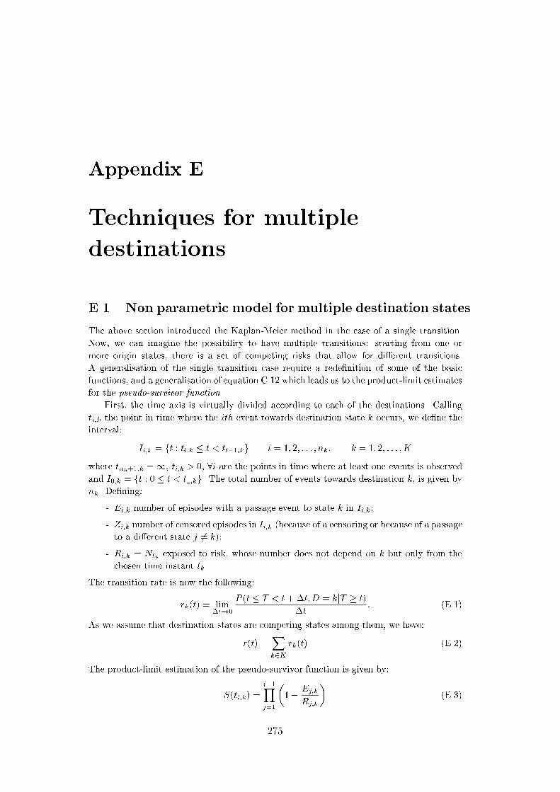
Appendix E
Techniques for multiple
destinations
E.1 Non parametric model for multiple destination states
The above section introduced the Kaplan-Meier method in the case of a single transition.
Now, we can imagine the possibility to have multiple transitions: starting from one or
more origin states, there is a set of competing risks that allow for di�erent transitions.
A generalisation of the single transition case require a rede�nition of some of the basic
functions, and a generalisation of equation C.12 which leads us to the product-limit estimates
for the pseudo-survivor function.
First, the time axis is virtually divided according to each of the destinations. Calling
ti;k the point in time where the ith event towards destination state k occurs, we de�ne the
interval:
Ii;k = ft : ti;k � t < ti+1;kg i = 1; 2; : : : ; nk; k = 1; 2; : : : ;K
where tnk+1;k =1, ti;k > 0, 8i are the points in time where at least one events is observed
and I0;k = ft : 0 � t < t1;kg. The total number of events towards destination k, is given by
nk. De�ning:
- Ei;k number of episodes with a passage event to state k in Ii;k ;
- Zi;k number of censored episodes in Ii;k (because of a censoring or because of a passage
to a di�erent state j 6= k);
- Ri;k = Ntk exposed to risk, whose number does not depend on k but only from the
chosen time instant tk.
The transition rate is now the following:
rk(t) = lim�t!0
P (t � T < t+�t;D = kjT � t)
�t: (E.1)
As we assume that destination states are competing states among them, we have:
r(t) =Xk2K
rk(t) (E.2)
The product-limit estimation of the pseudo-survivor function is given by:
S(ti;k) =
i�1Yj=1
�1�
Ej;k
Rj;k
�(E.3)
275

276 Appendix E. Techniques for multiple destinations
The reasoning is the same as the one presented for the single destination model.
E.1.1 Multiple origin and multiple destination states
To extend the concept just introduced to account for multiple origin and multiple destination
state, we need to consider duration of the events conditional on given origin states. To this
aim we need to de�ne the risk set which has to be speci�ed conditionally on the origin
state. Rj(t) is the risk set de�ned for all episode with origin state j provided that their
starting time is less than t and their ending time is equal or greater than t. The partial
likelihood function in the case of possibly more origin states and more destination states,
then becomes:
Lp =
Yj2O
Yk2Dj
Yi2Ejk
exp(�1X1(i) + �2X2(i) + : : :)Pi2R(t(i))
exp(�1X1(i) + �2X2(i) + : : :)(E.4)
If the time-dependent covariates change their values only at some discrete points in time,
the method of episode splitting can be used instead. The original episodes are split at every
point in time where one of the time-dependent covariates changes its value. Each of the
original episodes is replaced by a contiguous set of subepisodes (splits) with the appropriate
values of the covariates. the last of these splits has the same exit status as the original
episode: all other splits are regarded as right censored.

Bibliography
[1] Donald S. Akers. On measuring the marriage squeeze. Demography, 4(2):907{924,
1967.
[2] Paul D. Allison. Event history analysis. Quantitative Applications in the social sci-
ences. Sage, USA, 1991.
[3] Kiril F. Andreev. Demographic surfaces: Estimation, Assessment and Presentation,
with application to Danish Mortality, 18351995. Phd thesis, University of Southern
Denmark, 1999.
[4] Ruth Anshen. The Family: its function and destiny. Harper, New York, 1949.
[5] Maxine P. Atkinson and Becky L. Glass. Marital age heterogamy and homogamy.
Journal of marriage and the family, pages 685{691, August 1985.
[6] Marzio Barbagli. Provando e Riprovando. Contemporanea/35. Il Mulino, Bologna,
1990.
[7] Marzio Barbagli and Chiara Saraceno (eds.). Lo stato delle famiglie in Italia. Il
Mulino, Bologna, 1997.
[8] Fran�coise Bartiaux. D�enatalit�e et march�e matrimonial: le cas de l'Italie en 1930-1950.
Population, (1):91{118, 1994.
[9] Gary S. Becker. A theory of marriage, pages 299{344. In [167], 1974.
[10] Gary S. Becker. A treatise on the Family. Harvard University Press, Cambridge, 1981.
[11] Erik Beekink, Aart C. Liefbroer, and Frans van Poppel. Changes in choice of spouse
as an indicator of a society in a state of transition: Woerden, 1830-1930. Historical
Social Research, 23(1/2):231{253, 1998.
[12] Rodolfo Benini. Principi di Demogra�a. Barbera, Firenze, 1901.
[13] T.C. Bergstrom and M. Bagnoli. Courtship as a waiting game. Journal of Political
Economy, 101(1):185{202, 1993.
[14] Fabrizio Bernardi. Does the husband matter? married women and employment in
Italy. European Sociological Review, 15(3):285{300, 1999.
[15] Fabrizio Bernardi. Who marries whom in Italy: changes in educational homogamy
across cohorts and over the life-course. In [23], October 1999. forthcoming.
[16] Willem Bernasco. Coupled careers: the e�ects of spouse's resources on success at work.
PhD thesis, Universiteit te Utrecht, Amsterdam, 1994.
[17] Mari Bhat and Shiva S. Halli. Demography of the bridprice and dowry: causes and
consequences of the Indian marriage squeeze. Population Studies, (53):129{148, 1999.
277
278 BIBLIOGRAPHY
[18] Francesco C. Billari. L'analisi delle biogra�e e la transizione allo stato adulto. Aspetti
metodologici e applicazioni ai dati della Seconda Indagine sulla Fecondit�a in Italia.
Number 7 in Ricerche - Tesi di dottorato. CLEUP, Padova, 2000.
[19] Francesco C. Billari and Giuseppe A. Micheli. Social norms and demo-
graphic events in contemporary Western societies: can we learn from the
Southern Europe? October 1999. paper presented at the workshop on
Social Interactions and Demographic Behaviour, Rostock.
[20] Francesco C. Billari and G�otz Rohwer. Some developments in methods for life course
analysis and their applications, chapter 6, pages 323{334. Volume I of [168], 1998.
[21] Debra L. Blackwell. Marital homogamy in the united states: the in uence of individual
and paternal education. Social Science Research, (27):159{188, 1998.
[22] Hans-Peter Blossfeld and Alessandra De Rose. Educational expansion and changes
in entry into marriage and motherhood. the experience of Italian women. Genus,
(47):73{89, 1992.
[23] Hans-Peter Blossfeld and Andreas Timm (eds.). Who marries whom? Educational
systems as marriage markets in modern societies. Oxford University Press, Oxford,
1999. forthcoming.
[24] Hans-Peter Blossfeld and G�otz Rohwer. Techniques of events history modeling. New
approaches to causal analysis. Lawrence Erlbaum Associates, Mahwah, New Jersey,
1995.
[25] Hans-Peter Blossfeld and Johannes Huinink. Human capital investments or norms
of role transition? how women's schooling and career a�ect the process of family
formation. American Journal of Sociology, 97(1):143{168, July 1991.
[26] Alberto Bonaguidi (ed.). Migrazioni e demogra�a regionale in Italia. Franco Angeli,
Milano, 1985.
[27] Alberto Bonaguidi (ed.). Prospettive metodologiche nello studio della mobilit�a della
popolazione. Incontro di studio, Pisa, 13-14 ottobre 1988, Dipartimento di Statistica
e Matematica Applicata all'Economia, Universit�a. Pacini, Pisa, 1990.
[28] Corrado Bonifazi, Angela Chieppa, and Frank Heins. Le migrazioni interne merid-
ionali: un'analisi a livello provinciale, chapter 11, pages 53{95. Volume 10/99 of
Monogra�e [29], 1999.
[29] Corrado Bonifazi (ed). Mezzogiorno e migrazioni interne, volume 10/99 ofMonogra�e.
IRP-CNR, Roma, 1999.
[30] Michel Bozon. Les femmes et l'�ecart d'age entre conjoints: une domination consentie.
I: Types d'union et attentes en mati�ere d'�ecart d'age. Population, (2):327{360, 1990.
[31] Michel Bozon. Les femmes et l'�ecart d'age entre conjoints: une domination consen-
tie. II: Modes d'entr�ee dans la vie adulte et repr�esentations du conjoint. Population,
(3):565{602, 1990.
[32] Michel Bozon. Apparence physique et choix du conjoint, pages 91{110. Volume n.7 of
Congr�es et Colloques [101], 1991.
[33] Michel Bozon and Fran�coise H�eran. La d�ecouverte du conjoint. I: �evolution et mor-
phologie des sc�enes de rencontre. Population, (6):943{986, 1987.

BIBLIOGRAPHY 279
[34] Michel Bozon and Fran�coise H�eran. L'aire de recrutement du conjoint. Donn�ees
sociales, 1987.
[35] Michel Bozon and Fran�coise H�eran. La d�ecouverte du conjoint. II: les sc�enes de
rencontre dans l'espace social. Population, (1):121{150, 1988.
[36] L.J. Bumpass. What's happening to the family? interactions between demographic
and institutional change. Demography, (27):483{498, 1990.
[37] David M. Buss. The evolution of Desire: strategies of human mating. BasicBooks,
New York, 1994.
[38] J.C. Caldwell, P.H. Reddy, and Pat Caldwell. The causes of marriage change in
South India. Population Studies, (37):343{361, 1983.
[39] G. Cantisani and Gianpiero Dalla Zuanna. Nuzialit�a e famiglie complessse in Italia.
analisi territoriale di lungo periodo (1881-1981). Statistica, anno LVI(2):217{242, 1996.
[40] Graziella Caselli, Jacques Vallin, JamesW. Vaupel, and Anatoli I. Yashin. Age-speci�c
mortality trends in France and Italy since 1900: period and cohort e�ects. European
Journal of Population, 3:36{60, 1987.
[41] Graziella Caselli, James W. Vaupel, and Anatoli I. Yashin. Mortality in Italy: contours
of a century of evolution. Genus, 41(1-2):39{55, 1985.
[42] John B. Casterline, Lindy Williams, and Peter McDonald. The age di�erence between
spouses: variations among developing countries. Population Studies, (40):353{374,
1986.
[43] Maria Castiglioni. Una ricostruzione della popolazione residente in Italia per sesso,
et�a e stato civile, 1952-1981. Istituto di Ricerche sulla Popolazione - IRP, Roma, 1989.
[44] Maria Castiglioni. Analisi della nuzialit�a di�erenziale nelle generazioni di donne ital-
iane nate fra 1919 e 1968 utilizzando dati individuali retrospettivi. Number 1 in Tesi
di dottorato. Dipartimento Statistico, Universit�a degli studi di Firenze, Firenze, 1993.
[45] Maria Castiglioni. Analisi di�erenziale della nuzialit�a, chapter 22, pages 347{363. In
[65], 1999.
[46] Maria Castiglioni and Gianpiero Dalla Zuanna. Il matrimonio tardivo senza con-
vivenza. La formazione delle unioni in Italia negli anni 80, chapter 1, pages 13{41. In
Secondo Convegno dei Giovani Studiosi dei problemi di Popolazione [79], 1996.
[47] Alessandro Cavalli and Oliver Galland (eds.). L'allongement de la jeunesse. Actes
Sud, Paris, 1993.
[48] Alberto Cazzola. L'ingresso nella sessualit�a adulta, chapter 20, pages 311{326. In
[65], 1999.
[49] H.T. Christiansen. Timing of the �rst pregnancy as a factor in divorce: a cross-cultural
analysis. Eugenics Quarterly, September 1963.
[50] Luciano Ciucci and Filomena Racioppi (eds.). Studi di popolazione. Nuovi approcci per
la descrizione e l'interpretazione. Convegno dei Giovani Studiosi dei Problemi di Popo-
lazione. Dipartimento di Scienze Demogra�che, Universit�a degli studi di Roma\La
Sapienza", Roma, 1994, Roma, 2-4 giugno 1993.
[51] Ansley Coale and D.R. McNeil. The distribution by age of the frequency of �rst
marriage in a female cohort. Journal of the American Statistical Association, (67):743{
749, 1972.
280 BIBLIOGRAPHY
[52] Antonio Cobalti and Antonio Schizzerotto. La mobilit�a sociale in Italia. Il Mulino,
Bologna, 1994.
[53] James Coleman. Metatheory: explanation in Social Science, chapter 1, pages 1{23. In
[54], 1990.
[54] James S. Coleman. Foundations of social theory. MA: Harvard University Press,
Cambridge, 1990.
[55] Dave Collett. Modelling survival data in medical research. Text in Statistical Science.
Chapman and Hall, London, �rst edition, 1997.
[56] Randall Collins and Scott Coltrane. Sociology of marriage and the family: gender, love
and property. The Nelson-Hall series in Sociology. Nelson-Hall publishers, Chicago,
third edition, 1991.
[57] Bernardo Colombo. La conferenza di Bucarest sulla popolazione e il piano mondiale
d'azione. Le Scienze, (79), 1975.
[58] John Dagsvik. Aggregation in matching markets. Discussion paper, Statistics Norway,
Oslo, 1998.
[59] Leif Danziger and Shoshana Neuman. On the age at marriage: theory and evidence
from Jews and Moslems in Israel. Journal of Economic Behavior - Organization,
40:179{193, 1999.
[60] Kingsley Davis. The future of marriage, chapter 1, pages 25{52. In [61], 1985.
[61] Kingsley Davis (ed.). Contemporary Marriage: comparative perspective on a changing
institution. Russel Sage Foundation, New York, 1985.
[62] Alessandra De Rose and Cesidia Rufo. Il mercato matrimoiale in Italia. Evoluzione
della popolazione coniugabile e dei fattori di selezione della coppia, pages 41{71. In
Convegno dei Giovani Studiosi dei Problemi di Popolazione [50], 1994.
[63] Paolo De Sandre. Patterns of fertility in italy and factors of its decline. Genus,
LVI(1-2):19{54, 2000.
[64] Paolo De Sandre, Fausta Ongaro, Rosella Rettaroli, and Silvana Salvini. Matrimonio
e �gli: tra rinvio e rinuncia. Studi e Ricerche. Il Mulino, Bologna, 1997.
[65] Paolo De Sandre, Antonella Pinnelli, and Antonio Santini (eds.). Nuzialit�a e Fecondit�a
in trasformazione: percorsi e fattori del cambiamento. Il Mulino, Bologna, 1999.
[66] Fran�coise de Singly. Th�eorie critique de l'homogamie. L'Ann�ee sociologique, (37):181{
205, 1987.
[67] Andreas Diekmann. Di�usion and survival models for the process of entry into mar-
riage, chapter 9, pages 170{183. In [132], 1990.
[68] P. DiMaggio and J. Mohr. Cultural capital, educational attainment, and marital
selection. American Journal of Sociology, (90):1231{61, 1985.
[69] Hans-Peter Blossfeld (ed.). The new role of women. Family formation in modern
societies. Westview Press, 1995.
[70] T.J. Espenshade. Marriage trends in america: estimates, implications and underlying
causes. Population and Development Review, 11(2):193{245, June 1985.
[71] EUROSTAT. Yearbook '97. Eurostat, 1997.

BIBLIOGRAPHY 281
[72] Patrick Festy. Evolution de la nuptialit�e en Europe occidentale, depuis la guerre.
Population, (2):331{379, 1971.
[73] Oliver Galland. L'entr�ee dans la vie familiale, pages 11{18. In [47], 1993.
[74] Bradley A. Gambill, James W. Vaupel, and Anatoli I. Yashin. The lexis computer
program for creating shaded contour maps of the demographic surfaces. International
Insitute for Applied Systems Analysis, Working Paper(WP-86-37), August 1986.
[75] Janet Z. Giele and Glen H. Elder Jr. (eds.). Methods of life course research: qualitative
and quantitative approaches. Sage, London, 1998.
[76] Corrado Gini. Indici di omo�lia e di rassomoglianza. Atti del Regio Istituto Veneto,
pages 597{604, 1915.
[77] Paul Ginsborg. Il `miracolo economico', chapter 7, pages 283{343. In Gli Struzzi [78],
1989.
[78] Paul Ginsborg. Storia d'Italia dal dopoguerra ad oggi. Gli Struzzi. Einaudi, Torino,
1989.
[79] Piero Giorgi and Salvatore Strozza (eds.). Studi di popolazione. Temi di Ricerca Nuova.
Secondo Convegno dei Giovani Studiosi dei problemi di Popolazione. Dipartimento
di Scienze Demogra�che - Universita' di Roma \La Sapienza", Roma, Roma, 25-27
giugno 1996.
[80] Alain Girard. Le choix du conjoint: une enquete psycho-sociologique en France, volume
Cahier n.70 of Travaux et Documents. INED-PUF, Paris, third edition, 1981.
[81] D.V. Glass. Population in History: Essay in Historical Demography. Eversley D.E.C.,
London, 1965.
[82] Paul C. Glick. Fifty years of family demography: a record of social change. Journal
of Marriage and the Family, (50):861{873, November 1988.
[83] Paul C. Glick, David M. Herr, and John C. Bersford. Family formation and family
composition: trends and prospects, pages 30{40. In [178], second edition, 1963.
[84] Noreen Goldman, Charles F. Westo�, and Charles Hammerslough. Demography of
the marriage market in the United States. Population Index, (50):5{25, 1984.
[85] Frances Kobrin Goldscheider and Linda Waite. Sex di�erences in the entry into mar-
riage. American Journal of Sociology, 92(1):91{109, July 1986.
[86] Antonio Golini. Omogamia secondo il luogo d'origine in Italia. Atti della Riunione
Scienti�ca di Statistica, pages 219{247, 1961.
[87] Antonio Golini. Distribuzione della popolazione, migrazioni interne e urbanizzazione
in Italia. Istituto di Demogra�a, Rome, 1974.
[88] William J. Goode. The family. Foundations of Modern Sociology. Prentice-Hall, New
Jersey, 1964.
[89] E. Grebenik, C. H�ohn, and R. Mackensen (eds.). Later Phases of the Family Cycle.
IUSSP. Clarendon Press, Oxford, reprinted in 1996 edition, 1989.
[90] Margaret E. Greene and Vijayendra Rao. The marriage squeeze and the rise in informal
marriage in Brazil. Social Biology, 42(1-2):65{82, 1995.
282 BIBLIOGRAPHY
[91] Amyra Grossbard-Shechtman. Marriage Squeezes and the Marriage Market, chap-
ter 14, pages 375{395. In [61], 1985.
[92] M. Guttentag and P.F. Secord. Too many women? The Sex Ratio question. Sage,
Beverly Hills, 1983.
[93] J. Hajnal. European marriage patterns in perspective, chapter 6, pages 101{143. In
[81], 1965.
[94] Max Haller. Marriage, women and social strati�cation: a theoretical critique. Ameri-
can Journal of Sociology, 86(4):766{795, 1981.
[95] Ulrich P�otter and G�otz Rohwer. Introduction. March 1999.
[96] Louis Henry. Nuptiality. Theoretical population biology, (3):135{152, 1972.
[97] Louis Henry. Naissance d'une population de couples mari�es, pages 81{96. Volume 1-2
of [109], 1973.
[98] Louis Henry. Sch�ema d'�evolution des marriages apr�es de grandes variations des nais-
sances. Population, (4-5):759{780, 1975.
[99] Gudmund Hernes. The process of entry into �rst marriage. American Sociological
Review, 37:173{182, April 1972.
[100] David M. Herr and Amyra Grossbard-Shechtman. The impact of the female marriage
squeeze and the contraceptive revolution on the sex roles and the women's liberation
movement in the United States, 1960 to 1975. Journal of Marriage and the Family,
February 1981.
[101] Th�er�ese Hibert and Louis Roussel (eds.). La nuptialit�e: �evolution r�ecente en France at
dans les pays d�evelopp�es, volume n.7 of Congr�es et Colloques. INED-Puf, Paris, 1991.
[102] Jan M. Hoem. Concepts of a bisexual theory of marriage formation. Statistisk Tidskrift,
(4):295{300, 1969.
[103] Y. Hu and N. Goldman. Mortality di�erentials by marital status: an international
comparison. Demography, 27(2), 1990.
[104] ISTAT. La fecondit�a delle regioni italiane. Analisi per coorti. Anni 19952-1993. Num-
ber 35 in Informazioni. Istat, Roma, 1997.
[105] ISTAT. La fecondit�a nelle regioni italiane. analisi per coorti. anni 1952-1993. Infor-
mazioni, (35), 1997.
[106] ISTAT. Tavole di fecondit�a regionale. In Informazioni [104], 1997.
[107] ISTAT. Internal migration and regional population dynamics in Italy. Essays, n.3,
1998.
[108] ISTAT. Rapporto annuale 1999. Istat, Roma, 2000.
[109] IUSSP. International Population conference, volume 1-2. Liege, 1973.
[110] J.D. Kalb eisch and R.L. Prentice. A statistical analysis of failure time data. Wiley,
New York, 1980.
[111] Matthijs Kalmijn. Spouse selection among children of European immigrants: a com-
parison of marriage cohorts in the 1960 census. International Migration Review,
xxvii(1):5178, 1993.
BIBLIOGRAPHY 283
[112] Matthijs Kalmijn. Assortative mating by cultural and economic occupational status.
American Journal of Sociology, (100):422{452, 1994.
[113] Matthijs Kalmijn. Intermarriage and homogamy: causes, patterns, trends. Annual
Review of Sociology, 24:395{421, 1998.
[114] Matthijs Kalmijn and Paul M. de Graaf. Remarriage and cohabitation after divorce
in the Netherlands. paper presented at the conference `Population Studies in Britain
and the Netherlands' Utrecht, August 2000.
[115] E.L. Kaplan and P. Meier. Nonparametric estimation from incomplete observations.
Journal of American Statistical Association, (53):457, 1958.
[116] R.E. Kass and A.E. Raftery. Bayes factors. journal of American Statistical Association,
(90):773{795, 1995.
[117] M.C. Keeley. The economics of family formation. Economic Inquiry, XV:238{250,
April 1977.
[118] Nico Keilman. Demographic and discrete-choice two-sex marriage models. paper
presented at the workshop on Non-Linear Demography, Rostock, Germany, May 1998,
April 1998.
[119] K.C. Land and A. Rogers (eds.). Multidimensional Mathematical Demography. Aca-
demic Press, USA, 1982.
[120] Henri Leridon. Pourquoi le d�emographe s'int�eresse-t-il �a la nuptialit�e?, pages 7{18.
Volume n.7 of Congr�es et Colloques [101], 1991.
[121] Henri Leridon and Laurent Toulemon. Analyse des interf�erences, chapter 7, pages
91{104. In Collection �Economie et Statistiques Avanc�ees [122], 1997.
[122] Henri Leridon and Laurent Toulemon. D�emographie. Collection �Economie et Statis-
tiques Avanc�ees. Economica, Paris, 1997.
[123] Henry Leridon and Catherine Villeneuve-Gokalp (eds.). Constances and inconstances
de la famille. Travaux et Documents, Cahier n.134. Puf-INED, Paris, 1994.
[124] Ron Lesthaeghe and Johan Surkyn. Cultural dynamics and economic theories of
fertility change. Population and Development Review, 14(1):1{46, March 1988.
[125] Susan K. Lewis and Valerie K. Oppenheimer. Educational assortative mating across
marriage markets: non-Hispanic whites in the United States. Demography, 37(1):29{
40, February 2000.
[126] Daniel T. Lichter. Delayed marriage, marital homogamy, and the mate selection
process among white women. Social Science Quarterly, 71(4):802{811, December 1990.
[127] Daniel T. Lichter, Robert N. Anderson, and Mark D. Hayward. Marriage markets and
marital choice. Journal of Family Issues, 16(4):412{431, July 1995.
[128] Daniel T. Lichter, Diane K. McLaughlin, George Kephart, and David J. Landry. Race
and the retreat from marriage: a shortage of marriageable men? American Sociological
Review, (57):781{799, December 1992.
[129] Dick London. Survival models and their estimation. ACTEX Pubilactions, Winsted,
Connecticut, third edition edition, 1997.
[130] Robert D. Mare. Five decades of educational assortative mating. American Sociological
Review, 56:15{32, February 1991.
284 BIBLIOGRAPHY
[131] Ettore Marubini and Maria Grazia Valsecchi. Analysing survival data from clinical tri-
als and observational studies. Statistics in practice. John Wiley and Sons, Chichester,
England, 1995.
[132] Karl Ulrich Mayer and Nancy Brandon Tuma (eds.). Event history analysis in life
course research. The University of Wisconsin Press, Wisconsin, 1990.
[133] Peter McDonald. L'�equilibre num�erique entre hommes et femmes et le march�e matri-
monial. Population, pages 1579{1590, 1995.
[134] D.D. McFarland. Models of marrigae formation and fertility. Social Forces, (54):66{83,
1975.
[135] Giuseppe A. Micheli. Citt�a, circolazione, permanenza: ancora sulle implicazioni
teoriche e operative del concetto di mobilit�a, chapter I, pages 17{37. In Incontro di
studio, Pisa, 13-14 ottobre 1988, Dipartimento di Statistica e Matematica Applicata
all'Economia, Universit�a [27], 1990.
[136] Giuseppe A. Micheli. Pi�u transizioni in una, chapter 3, pages 73{89. In [137], 1995.
[137] Giuseppe A. Micheli (ed.). La societ�a del �glio assente. Franco Angeli, 1995.
[138] Alain Monnier. The demographic sistuation in Europe and the developed countries
overseas: an annual report. Population: An English Selection, 10(2):447{473, 1998.
[139] H.V. Muhsam. The marriage squeeze. Demography, 11(2):291{299, May 1974.
[140] Krishnan Namboodiri and C.M. Suchindran. Life table techniques and their applica-
tions. Studies in Population. Academic Press, Orlando, 1987.
[141] Valerie Kincade Oppenheimer. A theory of marriage timing. American Journal of
Sociology, 94(3):563{591, November 1988.
[142] Emma Otta, Renato da Silva Querioz, Lucila de Sousa Campos, Monika
Weronika Dowbor da Silva, and Mariana Telles Silveira. Age di�erences between
spouses in a Brazilian marriage sample. Evolution and Human Behavior, (20):99{103,
1999.
[143] Rossella Palomba (ed.). Vita di coppia e �gli. La Nuova Italia, Firenze, 1987.
[144] Talcott Parsons. The social structure of the family, pages 173{201. In [4], 1949.
[145] Antonella Pinnelli and Alessandra De Rose. Italy, chapter 8, pages 175{190. In [69],
1995.
[146] John Pollard. Modelling human populations for projections purposes- some of the
problems and challenges. Australian Journal of Statistics, (2):63{76, 1975.
[147] Zhenchao Qian and Samuel Preston. Changes in American marriage, 1972 to 1987:
availability and forces of attraction by age and education. American Sociological
Review, 58:482{495, August 1993.
[148] Kelly R. Ralley. A sthortage of marriageable men? a note on the role of cohabitation in
Black-White di�erences in marriage rates. American Sociological Review, 61:973{983,
December 1996.
[149] Alessandra Righi. La nuzialit�a, chapter III, pages 53{64. In [7], 1997.
[150] G�otz Rohwer and Ulrich P�otter. Tda user's manual. Technical Report Version 1,
Ruhr-Universit�a Bochum, Bochum, Germany, 1998.
BIBLIOGRAPHY 285
[151] G. Rosoli (ed.). Cent'anni di emigrazione italiana (1876-1976), chapter I, pages 9{63.
In [152], 1978.
[152] G. Rosoli (ed.). Un secolo di emigrazione italiana 1876-1976. Centro Studi Emi-
grazione, Roma, 1978.
[153] Louis Roussel. Types of marriage and frequency of divorce, chapter 2, pages 19{36. In
IUSSP [89], reprinted in 1996 edition, 1989.
[154] Louis Roussel. La famille en Europe Occidentale: divergences et convergences. Popu-
lation, (1):??, 1992.
[155] Linda Laura Sabbadini. Famiglia unipersonale, unione libera o matrimonio. In [143],
1987.
[156] Linda Laura Sabbadini. Le convivenze\more uxorio", chapter VI, pages 86{94. In [7],
1997.
[157] Linda Laura Sabbadini. Modelli di formazione e organizzazione della famiglia. paper
presented to the \Convegno Le famiglie interrogano le politiche sociali", organized by
Dipartimento per gli A�ari Sociali, Presidenza del Consiglio dei Ministri, Bologna,
Italy, March 1999.
[158] Antonio Santini, Sabrina Prati, Alessandra Righi, A. Brancatello, Romina Fraboni,
Alessandra Masi, R. Rodol�, and Marina Venturi. La primo nuzialit�a nelle regioni
italiane: tavole per coorte e per contemporanei. Paper presented to the `Giornate di
Studio della Popolazione', Firenze, Gennaio 1999.
[159] Jean-Paul Sardon. La primo-nuptialit�e f�eminine en Europe: �el�ements pour une ty-
pologie. Population, (4):855{892, 1992.
[160] Hans M.A. Schadee and Luisa Saviori. Il matrimonio e le frequentazioni delle classi
superiori. Polis, VII(1):45{68, Aprile 1993.
[161] Hans M.A. Schadee and Antonio Schizzerotto. Processi di mobilit�a maschili e femminili
nell'Italia contemporanea. Polis, IV(1):97{139, Aprile 1990.
[162] Robert Schoen. The armonic mean as the basis of a realistic two-sex marriage model.
Demography, 18(2):201{216, May 1981.
[163] Robert Schoen. Generalizing the Life Table Model to incorporate interactions between
the sexes, chapter 7, pages 385{443. In [119], 1982.
[164] Robert Schoen. Measuring the tightness of a marriage squeeze. Demography, 20(1):61{
78, February 1983.
[165] Robert Schoen. The Marriage Squeeze, chapter 8, pages 167{185. In The Plenum
Series on Demographic Methods and Population Analysis [166], 1988.
[166] Robert Schoen. Modeling Multigroup Populations. The Plenum Series on Demographic
Methods and Population Analysis. Plenum Press, New York, 1988.
[167] Theodore P. Schultz (ed.). Economics of the family: marriage, children and human
capital; a conference report of the National Bureau of Economic Research. University
of Chicago Press, Chicago, 1974.
[168] SIS. Atti della XXXIX riunione scienti�ca, volume I. SIS, Sorrento, 14-17 Aprile,
1998.
286 BIBLIOGRAPHY
[169] Wilma Smeenk. Opportunity and marriage: the impact of individual resources
and marriage market structure on �rst marriage timing and partner choice in
The Netherlands. PhD Thesis. Thela Thesis, 1998.
[170] Jeroen Smits, Wout Ultee, and Jan Lammers. Educational homogamyin 65 countries:
an explanation of di�erences in openess using country-level explanatory variables.
American Sociological Review, (63):264{285, 1998.
[171] Jeroen Smits, Wout Ultee, and Jan Lammers. More or less educational homogamy?
a test of di�eretn versions of modernization theory using cross-temporal evidence for
60 countries. American Sociological Review, pages 781{788, October 2000.
[172] E. Sori. L'emigrazione italiana dall'Unit�a alla seconda guerra mondiale, chapter II-III,
pages 19{118. In [173], 1979.
[173] E. Sori. L'emigrazione italiana dall'Unit�a alla seconda guerra mondiale. Il Mulino,
Bologna, 1979.
[174] Scott J. South and Kim M. Lloyd. Marriage markets and nonmarital fertility in the
United States. Demography, 29(2):247{264, May 1992.
[175] Scott J. South and Kim M. Lloyd. Marriage oportunities and family formation: further
implications of imbalanced sex ratios. Journal of marriage and the family, (54):440{
451, 1992.
[176] Scott J. South and Kim M. Lloyd. Spousal alternatives and marital dissolution. Amer-
ican Sociological Review, 60:21{35, February 1995.
[177] Haya Stier and Yossi Shavit. Age at marriage, sex ratios, and ethnic heterogamy.
European Sociological Review, 10(1):79{87, May 1994.
[178] Marvin B. Sussman (ed.). Sourcebook in marriage and the family. Houghton Mi�in,
Boston, second edition, 1963.
[179] Nancy Brandon Tuma and Michael T. Hannan. Social Dynamics: models and methods.
Quantitative studies in social relations. Academic Press, Orlando, 1984.
[180] Peter Uhlenberg and Teresa M. Cooney. Male and female physicians: family and
career comparisons. Social Science and Medicine, (30):373{78, 1990.
[181] U.N. Patterns of �rst marriage: Timing and prevalence. Department of international
economic and social a�airs, United Nations, New York, 1990.
[182] Wilfred Uunk. Who marries whom? the role of social origin, education and high
culture in mate selection of industrial societies during the twentieth century. PhD
thesis, Katholieke Universiteit Nijmegen, february 1996.
[183] Jacques Vallin and A. Nizard. La mortalit�e per �etat matrimonial. mariage s�election
ou mariage protection. Population, (32, Num�ero sp�ecial), 1977.
[184] Dirk J. Van De Kaa. Europe' Second Demographic Transiton, volume 42 of Population
Bulletin. Population Reference Bureau, Washington, 1987.
[185] Frans van Poppel, Aart C. Liefbroer, and Wendy J. Post. Vers un plus grande
homogamie d'age entre conjoints: di��erences entre les classes sociales et di��erences
r�egionales aux Pays-Bas, 1812-1912. Annales de D�emographie Historique, Le mariage,
r�egles et pratiques:73{110, 1998.
BIBLIOGRAPHY 287
[186] Hernan Vera, Donna H. Berardo, and Felix M. Berardo. Age heterogamy in marriage.
Journal of marriage and the family, pages 553{566, August 1985.
[187] Catherine Villeneuve-Gokalp. Du mariages aux unions sans papiers: histoire r�ecente
des transformations conjugales, page ? In Travaux et Documents, Cahier n.134 [123],
1994.
[188] Diana Vincenzi Amato. Il diritto di famiglia, chapter II, pages 37{52. In [7], 1997.
[189] Linda J. Waite. Does marriage matter? Demography, 32(4):483{507, November 1995.
[190] Guillame J. Wunsch and Marc G. Termote. Introduction to Demographic Analysis.
Principles and Methods. Plenum Press, New York, London, 1978.
[191] Kazuo Yamaguchi. Event History Analysis, volume 28 of Applied Social Research
Methods Series. Sage, New York, 1991.
[192] Zeng Yi, James W. Vaupel, and Anatoli I. Yashin. Marriage and fertility in China: a
Lexis-Surface analysis. International Insitute for Applied Systems Analysis, Working
Paper(WP-85-70), October 1985.


