ECEN 4652/5002 Communications Lab Spring 2017 1-16-17 P. Mathys Lab 1: Python Intro, Flat-Top PAM, PCM 1 Introduction 1.1 Baseband Signaling A simple communication scenario is the transmission of a text string over a waveform channel such as a pair of twisted wires or a wireless radio frequency (RF) link. Starting from simple baseband signaling over an ideal noiseless channel and later proceeding to more complicated situations, many important aspects of the theory and practice of communication engineering can be studied in this context. One goal of this lab is to introduce Python as a high-level tool for signal processing and, in particular, for the generation and reception of communication signals. Another goal is to be able to transmit and receive ASCII text strings in Python using flat-top PAM (pulse amplitude modulation) which is a simple baseband signaling technique. An extension of this is to use pulse code modulation (PCM) to also transmit analog message signals. Communication signals can be broadly divided into baseband signals and into bandpass signals (or passband signals). One way to define baseband and bandpass signals is as follows. Definition: A communication signal is called a baseband signal if the filter of smallest bandwidth (BW) that passes the signal essentially undistorted is a LPF (lowpass filter) with passband 0 ≤ f<f L . Conversely, if this filter of smallest BW is a BPF (bandpass filter) with passband 0 <f 1 <f<f 2 , then the corresponding signal is called a bandpass signal. 1.2 ASCII Code The ASCII (American Standard Code for Information Interchange) code is a 7-bit code for encoding upper/lower case characters from the English alphabet, as well as numbers, punctuation marks, and control characters. The following table shows all the possible 128 code sequences of the original ASCII code. 1
Transcript
ECEN 4652/5002 Communications Lab Spring 20171-16-17 P. Mathys
Lab 1: Python Intro, Flat-Top PAM, PCM
1 Introduction
1.1 Baseband Signaling
A simple communication scenario is the transmission of a text string over a waveform channelsuch as a pair of twisted wires or a wireless radio frequency (RF) link. Starting from simplebaseband signaling over an ideal noiseless channel and later proceeding to more complicatedsituations, many important aspects of the theory and practice of communication engineeringcan be studied in this context. One goal of this lab is to introduce Python as a high-level toolfor signal processing and, in particular, for the generation and reception of communicationsignals. Another goal is to be able to transmit and receive ASCII text strings in Python usingflat-top PAM (pulse amplitude modulation) which is a simple baseband signaling technique.An extension of this is to use pulse code modulation (PCM) to also transmit analog messagesignals.
Communication signals can be broadly divided into baseband signals and into bandpasssignals (or passband signals). One way to define baseband and bandpass signals is as follows.
Definition: A communication signal is called a baseband signal if the filter of smallestbandwidth (BW) that passes the signal essentially undistorted is a LPF (lowpass filter) withpassband 0 ≤ f < fL. Conversely, if this filter of smallest BW is a BPF (bandpass filter)with passband 0 < f1 < f < f2, then the corresponding signal is called a bandpass signal.
1.2 ASCII Code
The ASCII (American Standard Code for Information Interchange) code is a 7-bit codefor encoding upper/lower case characters from the English alphabet, as well as numbers,punctuation marks, and control characters. The following table shows all the possible 128code sequences of the original ASCII code.
1
7-Bit ASCII (American Standard Code for Information Interchange)
The first two columns consist of non-printable control characters, e.g., CR stands for carriagereturn and LF stands for line feed. The space character (ASCII code 0100000) is shown as SPin the table. In the teletype days transmissions typically started with a few synchronizationcharacters (SYN), followed by a start of text character (STX). After that the actual messagewould be sent and at the end terminated with an end of text character (ETX). The mainpurpose of characters like SYN, STX, and ETX was to synchronize the transmitting and thereceiving teletype machines.
The binary codes in the ASCII table above are shown with the MSB (most significant bit)on the left and the LSB (least significant bit) on the right. Because the wordlengths used incomputers are typically powers of 2, it is quite common to extend the ASCII code by addinga zero to the left of the MSB to make 8-bit codewords as shown in the following example.
2
“Test” in Extended (8-bit) ASCII
Character Extended ASCII Code
T 01010100
e 01100101
s 01110011
t 01110100
1.3 Parallel to Serial Conversion
Using the extended 8-bit ASCII code, the letter “T”, for instance, is encoded in binary as01010100. To transmit this 8-bit quantity in binary over a communication channel, each bitmust be read out and transmitted indivdually, according to a specific scheme that is knownto both the transmitter and receiver. The two most common schemes are to either read thebits out from left to right and therefore transmit MSB-first, or to read from right to leftand in this case transmit LSB-first. In either case the codeword for the first character issent first, followed by the codeword of the second character, etc.
The following two tables show the serial data sequence dn, n ≥ 0, for the string “Test” usingMSB-first and LSB-first parallel (8-bit) to serial conversion.
MSB-first Bit Sequence for “Test” (Extended 8-bit ASCII)
dn = 01010100 01100101 01110011 01110100
→ Index n increases from left to right →d0=0, d1=1, d2=0, d3=1, d4=0, d5=1, d6=0, d7=0, d8=0, d9=1, d10=1, . . .
LSB-first Bit Sequence for “Test” (Extended 8-bit ASCII)
dn = 00101010 10100110 11001110 00101110
→ Index n increases from left to right →d0=0, d1=0, d2=1, d3=0, d4=1, d5=0, d6=1, d7=0, d8=1, d9=0, d10=1, . . .
The spaces after every 8 bits are shown only for ease of reading. In an actual data transmis-sion all 32 bits would be sent consecutively, without any spaces or pauses.
In practice the LSB-first scheme is the one that is most commonly used for the transmissionof ASCII text.
1.4 Flat-Top PAM
Most physical communication channels, like twisted-pair wire, coaxial cable, free-space ra-dio frequency (RF) transmission, etc, are analog in nature. This implies in particular that
3
they require a continuous-time (CT) signal or waveform at the input. A discrete-time (DT)sequence, like dn in the ASCII examples of the previous section, therefore needs to be con-verted to a CT signal s(t) before it can be transmitted over a waveform channel. A simpleand straightforward rule, informally called “flat-top” PAM (pulse amplitude modulation),to obtain a waveform s(t) from dn with bit rate Fb = 1/Tb is to set
s(t) = dn , (n− 1/2)Tb ≤ t < (n+ 1/2)Tb .
In blockdiagram form, the function of a flat-top PAM transmitter is represented as shownin the following figure.
Flat-TopPAMDT sequence CT waveform
dn s(t)
The graph below shows the letter “C” (ASCII code 01000011) converted (LSB-first) to abinary flat-top PAM signal s(t).
Unipolar Binary Flat−Top PAM for String "C", Fb=1/T
b=100 bits/sec
A DT sequence dn, n ≥ 0, can also be expressed as
{dn} = {d0 δn + d1 δn−1 + d2 δn−2 + . . .} ,
where δk = 1 if k = 0 and δk = 0 otherwise. Each dm δn−m gets converted to a piece, from(m− 1/2)Tb to (m+ 1/2)Tb, of the signal s(t). Thus, another way to describe flat-top PAMmathematically is
s(t) =∞∑
n=0
dn p(t− nTb) ,
where dn is a binary sequence with bitrate Fb = 1/Tb, and p(t) is the rectangular pulse shownin the following figure.
4
p(t) =
{1 , −Tb/2 ≤ t < Tb/2 ,0 , otherwise .
p(t)
t
1
−Tb
2 0 Tb
2
1.5 Flat-Top PAM Receiver
In any communication system the task of the receiver is to reproduce the transmitted infor-mation as faithfully as possible. For flat-top PAM, the receiver initially simply consists of asampler that samples the received signal r(t) at times t = nTb, so that rn = r(nTb) as shownin the following blockdiagram.
• •↓t = nTb
r(t) rn
In the absence of noise and other channel degradations, r(t) ≈ s(t) and thus rn = d̂n, theestimate of the received sequence dn. In fact, setting r(t) = s(t),
d̂n = rn = s(t)∣∣t=nTb
=[ ∞∑
m=0
dmp(t−mTb)]∣∣∣t=nTb
=∞∑
m=0
dmp(nTb −mTb) .
Defining the sampled version of p(t) as
pn = p(nTb) =⇒ d̂n =∞∑
m=0
dm pn−m = dn ∗ pn .
Thus, the DT equivalent of PAM followed by sampling at the receiver is convolution betweenthe input sequence dn and the pulse samples pn, as shown in the next blockdiagram.
DT Equiv.hn = pn
dn d̂n
The rectangular pulse p(t) that is used for flat-top PAM satisfies pn = p(nTb) = δn andthus the DT convolution is trivial. But, as you will see later, the same DT equivalentblockdiagram can be used for PAM with more general p(t) and thus more general pn.
But suppose now that noise gets added to s(t) during the transmission and the receivedsignal becomes r(t) = s(t) + n(t), where n(t) is noise. An example of how r(t) might lookfor the letter “C” (8-bit ASCII, LSB-first) is shown in the graph below.
Unipolar Binary Flat−Top PAM with Noise for String "C", Fb=1/T
b=100 bits/sec
Now just sampling the received signal at the right time and converting it back to ASCII textwill not work because rn is a real number and not just 0 or 1. Thus, a decision device needsto be introduced after the sampler as shown in the blockdiagram below.
PAMp(t)
+
Noise n(t)
• • DecisionDevice↓
t = nTb
r(t)dn s(t) rn d̂n
The characteristic of the decision device is shown below. Assuming that the statistics ofpositive and negative noise levels are similar and that the noise is independent of the trans-mitted data, the threshold of the decision device is chosen halfway between the “legal” valuesof 0 and 1.
d̂n =
{0 , rn < 1/2 ,1 , rn ≥ 1/2 .
d̂n
rn
1
0 0.5 1
Note that, no matter how the threshold is chosen, errors will occur as the noise gets strongerand the signal-to-noise ratio (SNR) decreases. The structure of an optimum receiver thatmaximizes the SNR before using the decision device will be derived later on.
1.6 Pulse Code Modulation
Pulse code modulation (PCM) was invented by Alec Reeves in 1937 to obtain a digitalrepresentation of analog message signals m(t). In essence, m(t) is sampled at rate Fs samplesper second and then each sample is quantized to b bits which are in turn transmitted serially,e.g., using flat-top PAM. In telephony Fs = 8000 samples per second and b = 8 are the mostcommonly used parameters for individual subscriber lines, resulting in a binary signal with
6
bit rate Fb = 64 kbit/sec. One advantage of using PCM is that several signals can easily bemultiplexed in time so that they can share a single communication channel. A T1 carrier,for example, is used in telephony to transmit 24 multiplexed PCM signals with a total rateof 1.544 Mbit/sec (this includes some overhead for synchronization). A second advantageis that repeaters that need to be used to compensate for losses over large distances can(within some limits) restore the signal perfectly because only two signal levels need to bedistinguished.
Example: 3-Bit PCM for a Sinewave. The figure below shows a normalized sinewave(blue line) and its sampled and quantized version (red stem plot). A 3-bit quantizer withsign-magnitude output was used. The sign-magnitude format (rather than 2’s complement)reduces the sensitivity for small amplitude values to sign errors that may occur duringtransmission.
0 10 20 30 40 50 60−1
−0.8
−0.6
−0.4
−0.2
0
0.2
0.4
0.6
0.8
1
t/Ts
Code
000
001
010
011
100
101
110
111
Normalized Sine Sampled and Quantized to 3 Bits (Sign−Magnitude PCM)
The 6 graphs below show how the quantized samples of the sine signal are transmitted seriallyusing binary flat-top PAM. In this case the parallel to serial conversion is MSB first, i.e.,the sign bit is transmitted first and the LSB of the magnitude representation is transmittedlast.
7
0 1 2 3 4 5 6 7 8 9 100
0.5
1
3−Bit (Sign−Magnitude) PCM Signal Corresponding to Sine Signal
10 11 12 13 14 15 16 17 18 19 200
0.5
1
20 21 22 23 24 25 26 27 28 29 300
0.5
1
30 31 32 33 34 35 36 37 38 39 400
0.5
1
40 41 42 43 44 45 46 47 48 49 500
0.5
1
50 51 52 53 54 55 56 57 58 59 600
0.5
1
t/Ts
An interesting question is how to synchronize the receiver to the bit rate used at the trans-mitter when long strings of zeros or ones occur in the data. Several variations of the basicPCM scheme exist to deal with this problem, but their treatment is beyond the scope of thislab description.
Example: 3-Bit PCM for a Message Signal. The graph below shows a small segmentof a typical (normalized) speech message signal m(t) (blue line) and its digitized version (redstem plot) using 3-bit sign-magnitude format. It is quite visible that the 3-bit quantizationis too crude. In fact, since low amplitudes are much more common in speech signals thanhigh amplitudes, practical PCM schemes often use a non-linear quantization scheme.
8
0 10 20 30 40 50 60−1
−0.8
−0.6
−0.4
−0.2
0
0.2
0.4
0.6
0.8
1
t/Ts
Code
000
001
010
011
100
101
110
111
Normalized Message Signal m(t) Sampled and Quantized to 3 Bits (Sign−Magnitude PCM)
The conversion of the digitized message signal to a binary PCM signal is shown below.Again, the MSB-first rule was used for the parallel to serial conversion.
0 1 2 3 4 5 6 7 8 9 100
0.5
1
3−Bit (Sign−Magnitude) PCM Signal Corresponding to m(t)
10 11 12 13 14 15 16 17 18 19 200
0.5
1
20 21 22 23 24 25 26 27 28 29 300
0.5
1
30 31 32 33 34 35 36 37 38 39 400
0.5
1
40 41 42 43 44 45 46 47 48 49 500
0.5
1
50 51 52 53 54 55 56 57 58 59 600
0.5
1
t/Ts
The name “pulse code modulation” may seem a bit confusing, since PCM is really mostlya technique for digitizing analog signals and making them into binary data streams. It hasto be understood in the context of other techniques that were developed at about the sametime, for example pulse width modulation (PWM) and pulse position modulation (PPM).
9
1.7 Python and Jupyter Installation
The easiest way to get started with Python and Jupyter is to download and install Ana-conda from https://www.continuum.io/downloads. Anaconda installs Python, the JupyterNotebook, and commonly used packages for scientific computing, such as numpy, scipy, andmatplotlib. There are two different versions of Anaconda, one for Python 2.x and one forPython 3.x. For this course Python 3.x will work fine, but it is also possible to install both,the Python 2.x and the Python 3.x versions, on the same computer.
If you prefer to install Python and Jupyter separately, you can go tohttps://www.python.org/downloads/ for Python and afterwards tohttp://jupyter.readthedocs.io/en/latest/install.html (scroll down to “Installing Jupyter withpip”). If you already have Python installed you can directly go to the step of installingJupyter. To be able to use vectors and matrices efficiently, use signal processing functionssuch as filtering and fft, and make plots, you will also need numpy, scipy, and matplotlib,see https://www.scipy.org/install.html for instructions to install the SciPy stack.
1.8 Python Crash Course
Let’s use IPython (interactive Python) to generate 1 second of a sinusoidal waveform withsampling frequency Fs. We start by importing additional modules and setting parameters:
In [1]: from pylab import *
In [2]: Fs = 8000
In [3]: fm = 1000
In [4]: tlen = 1.0
In [5]: tt = arange(0,round(tlen*Fs))/float(Fs) # Time axis
Now suppose you want to change one of the parameters of the sinusoidal waveform, e.g., theduration tlen. In interactive mode you would have to change tlen and then run all of thesubsequent commands again (e.g., using the history command and copying and pasting.A better way is put the Python code for generating a sinusoidal waveform in a separatescript file (with extension .py) and then run the script in IPython. Here is the script filesine_1000.py for producing a sinusoidal waveform:
# File: sine_1000.py
# Generates 1.5 sec of 1000 Hz sinusoidal waveform
from pylab import *
# Parameters
Fs = 8000
fm = 1000
tlen = 1.5
# Generate time axis
tt = arange(0,round(tlen*Fs))/float(Fs)
# Generate sinewave
xt = sin(2*pi*fm*tt)
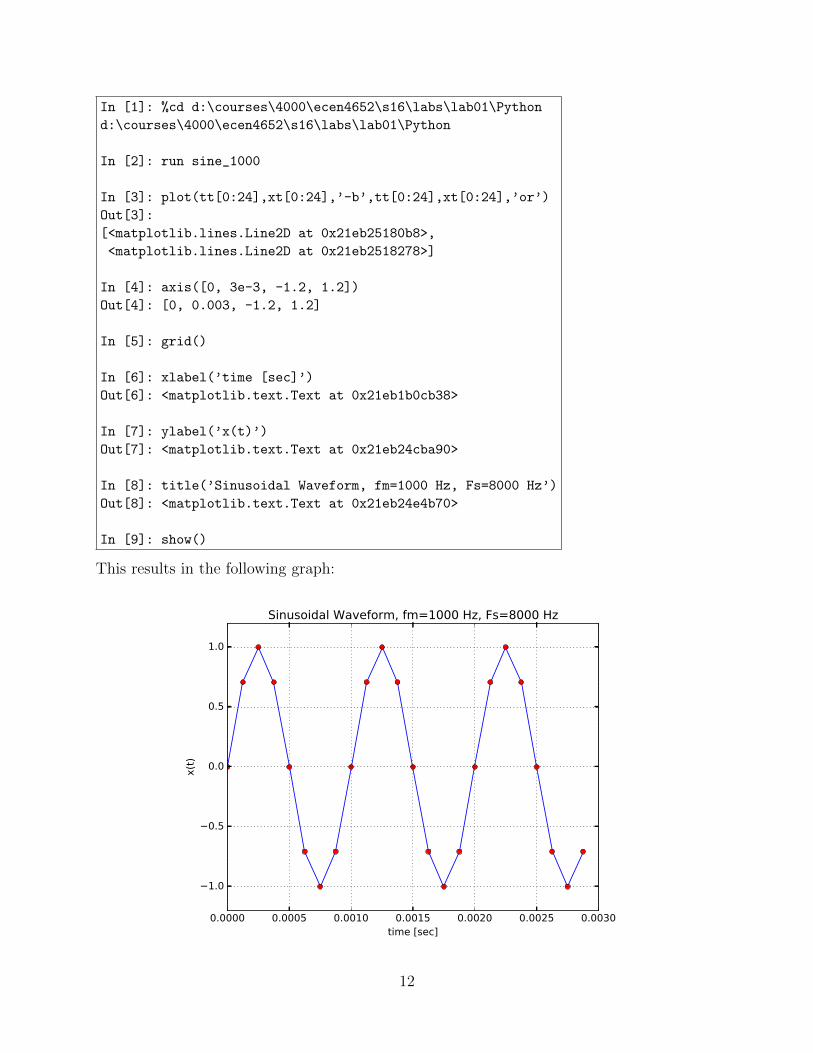
To obtain a graph in IPython we can run the following sequence of commands
11
In [1]: %cd d:\courses\4000\ecen4652\s16\labs\lab01\Python
d:\courses\4000\ecen4652\s16\labs\lab01\Python
In [2]: run sine_1000
In [3]: plot(tt[0:24],xt[0:24],’-b’,tt[0:24],xt[0:24],’or’)
Out[3]:
[<matplotlib.lines.Line2D at 0x21eb25180b8>,
<matplotlib.lines.Line2D at 0x21eb2518278>]
In [4]: axis([0, 3e-3, -1.2, 1.2])
Out[4]: [0, 0.003, -1.2, 1.2]
In [5]: grid()
In [6]: xlabel(’time [sec]’)
Out[6]: <matplotlib.text.Text at 0x21eb1b0cb38>
In [7]: ylabel(’x(t)’)
Out[7]: <matplotlib.text.Text at 0x21eb24cba90>
In [8]: title(’Sinusoidal Waveform, fm=1000 Hz, Fs=8000 Hz’)
Real and Imaginary Parts of Complex Exponential x(t)
xt.realxt.imag
You may have noticed that the 1000 Hz sinusoidal waveform we generated earlier doesn’tlook like a “nice” sinusoid because there are only 8 samples per period. A problem thatoften occurs in digital signal processing is that the sampling rate of a signal needs to beeither increased or decreased. To see how this can be done in Python we will use the 1000Hz sinusoidal signal and increase its sampling frequency from Fs = 8000 Hz to 3Fs = Fs3 =24000 Hz. The first step is to insert two zeros in-between any of the existing samples.
In [1]: %cd d:\courses\4000\ecen4652\s16\Labs\lab01\Python
d:\courses\4000\ecen4652\s16\Labs\lab01\Python
In [2]: run sine_1000
In [3]: stem(tt[0:24],xt[0:24]),grid()
Out[3]: (<Container object of 3 artists>, None)
In [4]: xlabel(’time [sec]’),ylabel(’xt’)
Out[4]:
(<matplotlib.text.Text at 0x276c12296d8>,
<matplotlib.text.Text at 0x276c1233e80>)
In [5]: title(’1000 Hz Sinusoid, Fs=8000 Hz’)
Out[5]: <matplotlib.text.Text at 0x276c12b2d68>
In [6]: show()
This produces a stem plot of the original sinewave.
To expand the signal xt 3-fold, insert two zeros after each sample by first constructing a2-dimensional array whose first row is xt and whose remaining two rows are all zeros. Thenreshape this array into a 1-dimensional vector, reading it out columns first (order=’F’ whereF stands for Fortran).
15
In [7]: x3at = vstack([xt, zeros(len(xt)), zeros(len(xt))]) # Expand 3x
In [8]: x3t = reshape(x3at,x3at.size,order=’F’) # Reshape into vector
The next step is to interpolate between the nonzero samples in accordance with the as-sumption that the original signal is bandlimited to frequencies less than Fs/2. We will usea truncated sinc pulse for the interpolation, corresponding to a lowpass filter with cutofffrequency fL. We will use the following function in the file sinc_ipol.py to generate theimpulse response of the interpolation filter.
# File: sinc_ipol.py
# Sinc pulse for Interpolation
from pylab import *
def sinc(Fs, fL, k):
# Time axis
ixk = int(round(Fs*k/float(2*fL)))
tth = arange(-ixk,ixk+1)/float(Fs)
# Sinc pulse
ht = 2.0*fL*ones(len(tth))
ixh = where(tth != 0.0)[0]
ht[ixh] = sin(2*pi*fL*tth[ixh])/(pi*tth[ixh])
return tth,ht
if __name__ == ’__main__’:
sinc()
The commands below show how the interpolation filter is generated.
17
In [16]: import sinc_ipol
In [17]: fL = 3000 # Cutoff frequency
In [18]: k = 10 # sinc pulse truncation
In [19]: tth,ht = sinc_ipol.sinc(Fs3, fL, k)
In [20]: plot(tth,ht,’m’),grid()
Out[20]: ([<matplotlib.lines.Line2D at 0x276c15935f8>], None)
In [21]: xlabel(’time [sec]’),ylabel(’h(t)’)
Out[21]:
(<matplotlib.text.Text at 0x276c1550400>,
<matplotlib.text.Text at 0x276c155aa90>)
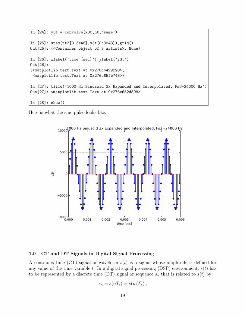
In [22]: title(’sinc Pulse for Interpolation, Fs3=24000 Hz, fL=3000 Hz, k=10’)
1000 Hz Sinusoid 3x Expanded and Interpolated, Fs3=24000 Hz
1.9 CT and DT Signals in Digital Signal Processing
A continous time (CT) signal or waveform s(t) is a signal whose amplitude is defined forany value of the time variable t. In a digital signal processing (DSP) environment, s(t) hasto be represented by a discrete time (DT) signal or sequence sn that is related to s(t) by
sn = s(nTs) = s(n/Fs) ,
19
where Fs = 1/Ts is the sampling rate in Hz. As an example, consider the sinusoid
s(t) = sin 2πf0t .
Setting f0 = 100 Hz and Fs = 700 Hz and plotting sn versus t = nTs yields the followinggraph.
Even though the sampling theorem is not violated (Fs > 2f0), the plot (with straight linesbetween samples) is clearly not a very good approximation to s(t). In such a case it isactually better to just simply plot the DT signal sn versus n in the form of a stem plot asshown in the next figure.
0 5 10 15 20 25 30 35−1
−0.5
0
0.5
1
n
s n
100 Hz DT Sinewave, Fs = 700 Hz
However, if Fs is chosen much larger than 2f0, then a plot of sn versus t = nTs is a veryclose approximation to plotting s(t) versus t, as can be easily seen in the graph below (whichuses Fs = 5000 Hz and does not explicitly show the sampling points).
In general, a signal vector s in a DSP environment with bandlimitation to fB Hz will beconsidered a DT signal sn if the sampling rate Fs (in Hz) is not much higher than the Nyquistrate 2fB, and it will be considered (a good approximation to) a CT signal s(t) if Fs � 2fB.
2 Lab Experiments
E1. Signals in Python. Assume that s(t) is a bandlimited CT signal that is to berepresented in Python by a DT sequence sn with sampling rate Fs = 1/Ts. According tothe sampling theorem, Fs must be at least twice the highest frequency in s(t), but howshould Fs be chosen so that a plot of sn looks like s(t)? The goal of this experiment is togain some intuitive experience for this question and at the same time practice some Pythonprogramming.
(a) Make a script file called sine100.py, using the following (numpy) Python commands:
# File: sine100.py
# Asks for sampling frequency Fs and then generates
# and plots 5 periods of a 100 Hz sinewave
from pylab import *
from ast import literal_eval
Fs = literal_eval(input(’Enter sampling rate Fs in Hz: ’))
f0 = 100 # Frequency of sine
tlen = 5e-2 # Signal duration in sec
tt = arange(0,round(tlen*Fs))/float(Fs) # Time axis
st = sin(2*pi*f0*tt) # Sinewave, frequency f0
This creates a discrete time axis tt of duration tlen with time instants spaced 1/Fs secondsapart. The last statement generates the signal st which is a 100 Hz sine, sampled with rateFs. Plot st versus tt for Fs equal to 200, 400, 800, 1600, 3200, etc. What is the smallest Fsthat yields a “nice” and representative graph of a 100 Hz CT sinusoid? Look at the samplegraphs shown in the introduction.
(b) After generating the sine in st, use the command
21
rt = sign(st) # Sine -> rectangular
to generate a rectangular signal rt with frequency 100 Hz and sampling rate Fs. Note thatsign stands for the signum function which is defined as
sgn(x) =
+1 , x > 0 ,0 , x = 0 ,−1 , x < 0 .
Plot rt versus tt for Fs equal to 200, 400, 800, 1600, 3200, etc. What is the smallest Fs
that yields a “nice” and representative graph of a 100 Hz rectangular CT signal?
(c) DT approximations to CT signals in Python can be differentiated and integrated, whichis often useful for the generation and anlysis of communication signals. Again, the goodnessof the approximation of a CT signal by its sampled counterpart depends on the choice of thesampling frequency Fs. The following table shows the (numpy) Python commands for theDT approximations to differentiation and integration of a CT signal x(t).
Derivative and Integral of Signals
CT Signal x(t) DT Signal x
Derivativedx(t)
dtdiff(hstack((0,x)))*Fs
Integral∫dx(t) dt cumsum(x)/float(Fs)
Note that since the sampling rate is Fs, “dt” is equal to Ts=1/Fs. Generate a rectangular100 Hz signal in rt as in part (b) and then use the following commands to generate the“derivative” rdt of rt and the “integral” rdit of rdt which should be rt again.
rdt = diff(hstack((0,rt)))*Fs # Derivative of rt
rdit = cumsum(rdt)/float(Fs) # Integral of rdt
Make plots of rdt and rdit with Fs at the lower end of the useful range first so that youcan see what diff and cumsum are doing. Then increase Fs until you obtain a plot that isa “nice” and representative approximation to differentiation and integration of CT signals.The following graphs show an example when Fs=900 Hz.
22
0.00 0.01 0.02 0.03 0.04 0.052000
1500
1000
500
0
500
1000
1500
2000
dr(
t)/d
t
Derivative of 100 Hz Rectangular Wave, Fs = 900 Hz
0.00 0.01 0.02 0.03 0.04 0.05time [sec]
1.0
0.5
0.0
0.5
1.0
∫ dr(
t)/d
t
Integral of Derivative of 100 Hz Rectangular Wave, Fs = 900 Hz
(d) The graph below shows the samples of a signal called sig01. This signal is available insig01.wav. Use the wavread function in the Appendix to read the .wav file.
0.000 0.005 0.010 0.015 0.020−1.0
−0.5
0.0
0.5
1.0Samples of a Signal
Make a plot of the “CT version” of sig01, assuming that sig01 is a baseband signal. Explainyour approach and specify the parameters that you used.
E2. Flat-Top PAM. (a) The goal of the first part of this experiment is to write a Pythonscript file, e.g., called ftpam01.py, that accepts a text string as input and produces a flat-topPAM signal st as output. Here is an outline of ftpam01.py:
23
# File: ftpam01.py
# Script file that accepts an ASCII text string as input and
# produces a corresponding binary unipolar flat-top PAM signal
# s(t) with bit rate Fb and sampling rate Fs.
# The ASCII text string uses 8-bit encoding and LSB-first
# conversion to a bitstream dn. At every index value
# n=0,1,2,..., dn is either 0 or 1. To convert dn to a
# flat-top PAM CT signal approximation s(t), the formula
# s(t) = dn, (n-1/2)*Tb <= t < (n+1/2)*Tb,
# is used.
from pylab import *
import ascfun as af
Fs = 44100 # Sampling rate for s(t)
Fb = 100 # Bit rate for dn sequence
txt = ’Test’ # Input text string
bits = 8 # Number of bits
dn = # >> Convert txt to bitstream dn here <<
N = len(dn) # Total number of bits
Tb = 1/float(Fb) # Time per bit
ixL = round(-0.5*Fs*Tb) # Left index for time axis
ixR = round((N-0.5)*Fs*Tb) # Right index for time axis
tt = arange(ixL,ixR)/float(Fs) # Time axis for s(t)
st = # >> Generate flat-top PAM signal s(t) here <<
Hints: The following Python module can be used to convert a text string in txt to ASCIIusing bits bits per character and then to a serial bitstream in dn (and vice versa).
24
# File: ascfun.py
# Functions for conversion between ASCII and bits
from pylab import *
def asc2bin(txt, bits=8):
"""
ASCII text to serial binary conversion
>>>>> dn = asc2bin(txt, bits) <<<<<
where txt input text string
abs(bits) bits per char, default=8
bits > 0 LSB first parallel to serial
bits < 0 MSB first parallel to serial
dn binary output sequence
"""
txtnum = array([ord(c) for c in txt]) # int array
if bits > 0: # Neg powers of 2, increasing exp
p2 = np.power(2.0,arange(0,-bits,-1))
else: # Neg powers of 2, decreasing exp
p2 = np.power(2.0,1+arange(bits,0))
B = array(mod(array(floor(outer(txtnum,p2)),int),2),int8)
# Rows of B are bits of chars
dn = reshape(B,B.size)
return dn # Serial binary output
def bin2asc(dn, bits=8, flg=1):
"""
Serial binary to ASCII text conversion
>>>>> txt = bin2asc(dn, bits, flg) <<<<<
where dn binary input sequence
abs(bits) bits per char, default=8
bits > 0 LSB first parallel to serial
bits < 0 MSB first parallel to serial
flg != 0 limit range to [0...127]
txt output text string
"""
# >>Function to be completed in part (b)<<
To generate st from dn you might consider using the differentiation/integration techniquefrom E1(c) by differentiating dn, placing the resulting impulses spaced apart by Tb at t =−Tb/2, Tb/2, 3Tb/2, 5Tb/2, . . . in st and then integrating over st to obtain a rectangularflat-top PAM signal. The graph below shows st for the text string Test.
When you have completed the code in ftpam01 and you have verified that it works correctly,generate a known test signal, e.g., with txt=’MyTest’ and save the resulting signal st in awav file using the commands (see the wavfun module in the Appendix)
so that you can use it in the second part of the experiment. Note that the amplitude A ofsignals in wav-files is restricted toA < 1 and for this reason 0.999*st/float(max(abs(st)))
is written with the wavwrite command rather than just st.
(b) The goal of this part of the experiment is to take a received flat-top PAM signal rt of thekind generated in (a) and to convert it back to a text string. It is assumed that the receivedsignal rt is available in the form of a wav file. Here is the starting point for a flat-top PAMreceiver script file called ftpam_rcvr01:
26
# File: ftpam_rcvr01.py
# Script file that accepts a binary unipolar flat-top PAM
# signal r(t) with bitrate Fb and sampling rate Fs as
# input and decodes it into a received text string.
# The PAM signal r(t) is received from a wav-file with
# sampling rate Fs. First r(t) is sampled at the right
# result is then quantized to binary (0 or 1) to form the
# estimated received sequence dnhat which is subsequently
# converted to 8-bit ASCII text.
from pylab import *
import ascfun as af
import wavfun as wf
rt, Fs = wf.wavread(’MyTest.wav’)
Fb = 100 # Data bit rate
Tb = 1/float(Fb) # Time per bit
bits = 8 # Number of bits/char
N = floor(len(rt)/float(Fs)/Tb) # Number of received bits
dnhat = # >>Sample and quantize the received PAM signal here<<
txthat = # >>Convert bitstream dnhat to received text string<<
print(txthat) # Print result
Note: Because s(t) is obtained from dn with bit rate Fb = 1/Tb by setting
s(t) = dn , (n− 1/2)Tb ≤ t < (n+ 1/2)Tb ,
the first sample of the received signal in the wav file is at time t = −Tb/2 and not at timet = 0. Also, the signal in a 16-bit wav file may be scaled because the amplitude A has tosatisfy A < 1.
Test your receiver with the MyTest.wav file that you generated in (a). When you haveverified that your receiver works properly, use it to receive the signal in ftpam_sig01.wav
and convert it back to a text string. The bit rate that was used for this signal is Fb = 100.
(c) Use your ftpam_rcvr01 receiver to receive the signals in ftpam_sig02.wav and inftpam_sig03.wav and convert them back to text strings. The bit rate of the second signalin ftpam_sig02.wav is unknown and you have to determine it from the signal itself. Howdifficult is it to find the bit rate and how crucial is it to have exactly the right value? Thesignal in ftpam_sig03.wav uses a bit rate of Fb = 100 and noise has been added to it. Torecord it as a wav file it had to be scaled to have a maximum amplitude less than 1 (includingnoise), so it is crucial that you use the right threshold at the receiver.
E3. Pulse Code Modulation. (Experiment for ECEN 5002, optional for ECEN 4652) (a)Complete the following Python module with the mt2pcm and pcm2mt functions as describedbelow:
27
# File: pcmfun.py
# Functions for conversion between m(t) and PCM representation
from pylab import *
def mt2pcm(mt, bits=8):
"""
Message signal m(t) to binary PCM conversion
>>>>> dn = mt2pcm(mt, bits) <<<<<
where mt normalized (A=1) "analog" message signal
bits number of bits used per sample
dn binary output sequence in sign-magnitude
form, MSB (sign) first
"""
# >>Your code goes here<<
def pcm2mt(dn, bits=8):
"""
Binary PCM to message signal m(t) conversion
>>>>> mt = pcm2mt(dn, bits) <<<<<
where dn binary output sequence in sign-magnitude
form, MSB (sign) first
bits number of bits used per sample
mt normalized (A=1) "analog" message signal
"""
# >>Your code goes here <<
The function mt2pcm is used to convert the (unquantized) samples of a message signal mt toa PCM bit string dn with bits bit quantization per sample. The function pcm2mt is usedto convert the bit string dn back to “analog” samples. Test the two functions by using asine signal for m(t) in mt2pcm, then feeding the resulting dn into pcm2mt and finally plottingthis result together with the original m(t) in the same graph. Use a frequency of ≈ 100 Hzand a sampling rate in the range 4000 . . . 8000 Hz for the sine signal. Try 3-bit and 8-bitquantization.
(b) The signals in the files pcm_sig01.wav and pcm_sig02.wav are PCM signals with abitrate of 64 kbit/sec, using 8-bit quantization, sign-magnitude format and MSB-first trans-mission. Flat-top PAM was used to convert the bit squences dn to a CT signal with amplitudezero for dn=0 and positive amplitude for dn=1. The first signal is noiseless and the secondsignal has noise added to it. Note that the noisy signal had to be scaled to have an ampli-tude less than 1. Demodulate the two signals and convert them back to “analog” messagesignals. Write the m(t) signals to a wav-file, listen to them in a sound player and describetheir content. Use the PCM test signals in pcm_test01.wav and pcm_test02.wav to testyour PCM receiver. The first test signal is a 3-bit (sign-magnitude, MSB first) PCM signalwith bit rate Fb = 24000 and the second test signal is a 8-bit (sign-magnitude, MSB first)PCM signal. The message signal m(t) is in both cases a sine with frequency f = 233.3 Hz.
28
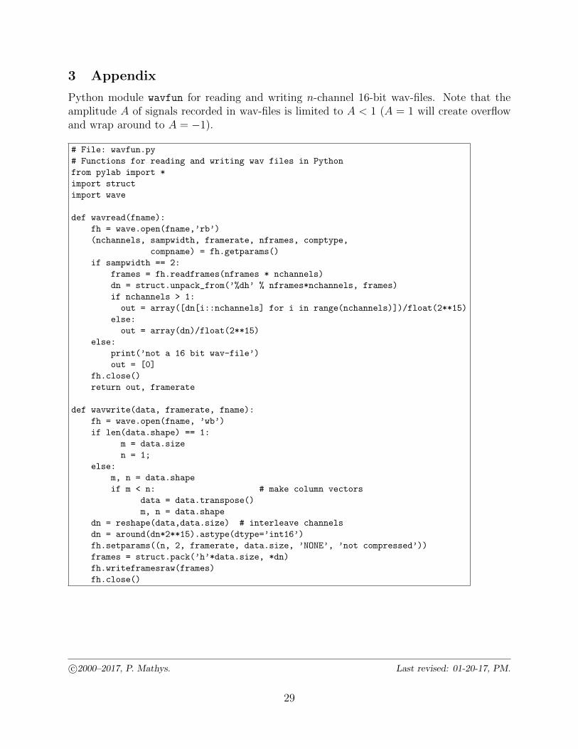
3 Appendix
Python module wavfun for reading and writing n-channel 16-bit wav-files. Note that theamplitude A of signals recorded in wav-files is limited to A < 1 (A = 1 will create overflowand wrap around to A = −1).
# File: wavfun.py
# Functions for reading and writing wav files in Python