CPE 311 UNIT OPERATIONS LABORATORY I March 22 Lab 3: Flocculation and Filtration Flocculation and filtration represent important unit operations for the separations of solids suspended in liquids. Location: EGB 67C – Unit Operations Laboratory References: TAPPI Standard Method T-261 . Samples: A sample suspension will be provided for you. It contains organic fibers and a fine particulate mineral. The approximate solid content is more than 0.5%. It must be diluted to complete the lab. Objectives: After this laboratory exercise students will be able to: • Plan, set up, execute and analyze the data from a 2 3 factorial experiment. • Set up and use a dynamic drainage (Britt) jar to determine fine particle retention. • Set up and use a dynamic drainage (Britt) jar to perform fines fractionation of a suspension. Synopsis: In this lab exercise, your group will use a factorial experimental design to investigate the relationship between fine particle flocculation (retention) and three important variables: mixing intensity, polymer concentration and mixing time. The advantages of experimental design for reducing testing effort while maximizing insight into simple trends, interactions between parameters and experimental error will be explored. Test will be conducted using standard methods based on the dynamic drainage (Britt) jar. Background: Flocculation of fine particles is an important unit operation used for the efficient separation of suspended solids from solutions. It is especially useful for isolating particles whose size falls into the colloidal range with diameters, D<5 µm. If sedimentation is to be used for separation, density difference between the particle and the liquid, = (p -L ), and particle diameter, D, contribute positively to the separation rate, V g , by Stokes law, cf. eq 1. This has important implications for the efficiency of a process.
Transcript
CPE 311 UNIT OPERATIONS LABORATORY I April 23
Lab 3: Flocculation and FiltrationFlocculation and filtration represent important unit operations for the separations of solids suspended in liquids.
Location: EGB 67C – Unit Operations Laboratory
References: TAPPI Standard Method T-261.
Samples: A sample suspension will be provided for you. It contains organic fibers and a fine par-ticulate mineral. The approximate solid content is more than 0.5%. It must be diluted to complete the lab.
Objectives: After this laboratory exercise students will be able to:• Plan, set up, execute and analyze the data from a 23 factorial experiment.• Set up and use a dynamic drainage (Britt) jar to determine fine particle retention.• Set up and use a dynamic drainage (Britt) jar to perform fines fractionation of a sus-
pension.
Synopsis: In this lab exercise, your group will use a factorial experimental design to investigate the relationship between fine particle flocculation (retention) and three important variables: mixing intensity, polymer concentration and mixing time. The advantages of experimental design for reducing testing effort while maximizing insight into simple trends, interactions between parameters and experimental error will be explored. Test will be conducted using standard methods based on the dynamic drainage (Britt) jar.
Background: Flocculation of fine particles is an important unit operation used for the efficient separation of suspended solids from solutions. It is especially useful for isolating particles whose size falls into the colloidal range with diameters, D<5 µm. If sedimentation is to be used for separation, density difference between the particle and the liquid, = (p -L), and particle diameter, D, contribute positively to the separation rate, Vg, by Stokes law, cf. eq 1. This has important implications for the efficiency of a process.
Vg = D2 (p - 1) G / 18µ eq1.
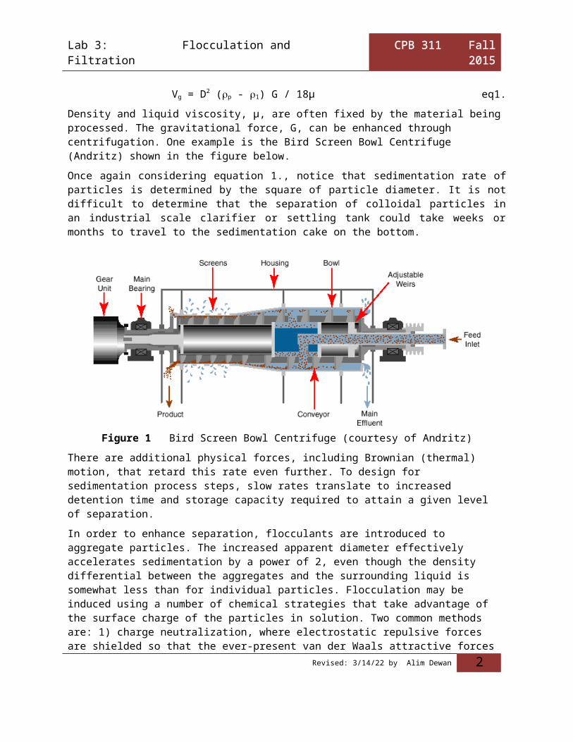
Density and liquid viscosity, µ, are often fixed by the material being processed. The gravitational force, G, can be enhanced through centrifugation. One example is the Bird Screen Bowl Centrifuge (Andritz) shown in the figure below.
Once again considering equation 1., notice that sedimentation rate of particles is determined by the square of particle diameter. It is not difficult to determine that the separation of colloidal particles in an industrial scale clarifier or settling tank could take weeks or months to travel to the sedimentation cake on the bot -tom.
Lab 3: Flocculation and Filtration CPB 311 Fall 2015
Figure 1 Bird Screen Bowl Centrifuge (courtesy of Andritz)
There are additional physical forces, including Brownian (thermal) motion, that retard this rate even fur-ther. To design for sedimentation process steps, slow rates translate to increased detention time and stor-age capacity required to attain a given level of separation.
In order to enhance separation, flocculants are introduced to aggregate particles. The increased apparent diameter effectively accelerates sedimentation by a power of 2, even though the density differential be-tween the aggregates and the surrounding liquid is somewhat less than for individual particles. Floccula-tion may be induced using a number of chemical strategies that take advantage of the surface charge of the particles in solution. Two common methods are: 1) charge neutralization, where electrostatic repulsive forces are shielded so that the ever-present van der Waals attractive forces cause particles to coagulate, and 2) the addition of charged polymers at electrostatically bind particles to form semi-rigid flocs. The latter method offers the advantages of better control and effectiveness. This laboratory exercise will pro-vide you the opportunity to characterize how process variables (mixing time and turbulence) and polymer concentration affect the performance of a commercial flocculant (also known as a retention aid in paper-making).
The specific flocculant that you will use in this lab takes utilizes the anionic (negative) charge on the sur-face of suspended particles by reacting with cationic (positive) charges that are distributed along a long chain, high molecular weight polymer. When the chain attaches to two or more particles, these particles are bridged together to form a cohesive floc that has some resistance to turbulent flow. If an excessive amount of the polymer is added, then the polymer coats all of the particle surfaces and no bridging be-tween particles occurs. Therefore, depending on the surface chemistry of the particles, the specific surface area exposed to the liquid, the solids concentration, and the solution chemistry, there is an optimal con-centration of flocculant additive that will maximize the flocculation of discrete particles. It is essential that the chemical be uniformly blended into the system so that all particles are collected. However, exces-sive mixing can also cause the flocs to break down. Thus, a balance between mixing time and intensity needs to be found in order to optimize performance of a flocculant additive.
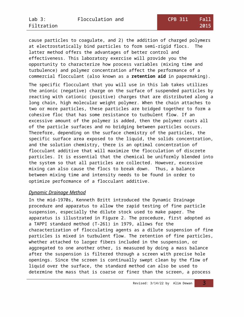
Dynamic Drainage MethodIn the mid-1970s, Kenneth Britt introduced the Dynamic Drainage procedure and apparatus to allow the rapid testing of fine particle suspension, especially the dilute stock used to make paper. The apparatus is illustrated in Figure 2. The procedure, first adopted as a TAPPI standard method (T-261) in 1979, allows for the characterization of flocculating agents as a dilute suspension of fine particles is mixed in turbulent flow. The retention of fine particles, whether attached to larger fibers included in the suspension, or ag-
Revised: 4/18/23 by Alim Dewan 2
Lab 3: Flocculation and Filtration CPB 311 Fall 2015
gregated to one another other, is measured by doing a mass balance after the suspension is filtered through a screen with precise hole openings. Since the screen is continually swept clean by the flow of liquid over the surface, the standard method can also be used to determine the mass that is coarse or finer than the screen, a process referred to as fractionation. The apparatus, known as a Dynamic Drainage Jar, (DDJ or Britt Jar), is custom made and specifically designed for testing drainage and retention. It is most commonly used in industry to test the performance of flocculating agents known as retention aids, as briefly describe above. In this lab session, you will use the DDJ to test the synergistic interactions be-tween flocculant concentration, mixing speed (turbulent intensity), and mixing time. Performance will be based on balance between those fines that are captured during filtration and those that remain dispersed and pass through the filtration screen.
In dealing with multi-variable systems, experimental design is used to apply logical patterns in order to draw valid conclusions from test array that varies each parameter. One goal is to maximize insight into the relationships between factors and the occurrence of any trends or interdependencies that might exist, while minimizing the required number of tests in the experiment. You should recognize the value of ex-perimental design as it allows you to vary several factors at a time and obtain valid results using a
Figure 2 Dynamic Drainage Jar, also known as the Britt Jar (courtesy of Paper Research Materials Inc.)
minimal amount of time and effort to perform the experiments. In this laboratory exercise, you will use the Factorial Design method to characterize the three variables important to drainage and retention.
Factorial DesignFactorial design is one of the more common forms of experimental design that is used to study processes with two or more variables (factors). Two important questions to ask when setting up a factorial design experiment are:
1) How many variables significantly influence the process? and 2) How many step differences or levels will each variable need testing?
If the answer to the second question is “more than two levels” than one use a general full factorial design, which can be a bit complex. If only two levels, say low and high, are tested for each variable, then a two level factorial design (2k design) is used. You will use this efficient design to examine the three variables in the drainage and retention experiment in what is referred to as a two-level, three-factor factorial design or simply “23 design”.
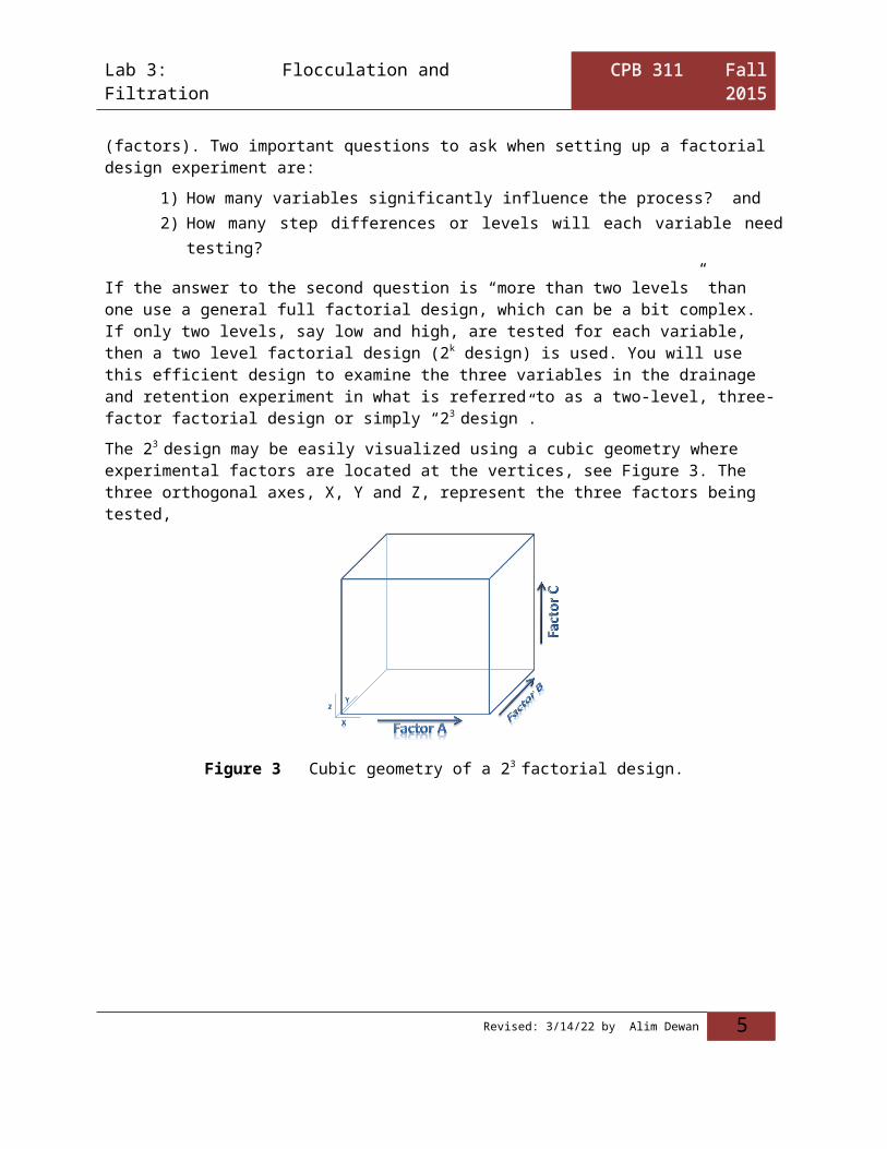
The 23 design may be easily visualized using a cubic geometry where experimental factors are located at the vertices, see Figure 3. The three orthogonal axes, X, Y and Z, represent the three factors being tested,
Revised: 4/18/23 by Alim Dewan 3
Lab 3: Flocculation and Filtration CPB 311 Fall 2015
Figure 3 Cubic geometry of a 23 factorial design.
AH
AL AH
AH
AH
AL
AL
AL
BH
BL
BH
BH
BL
BL
BL
BH
CL
CH
CL
CH
CH CH
CL CL
A B C
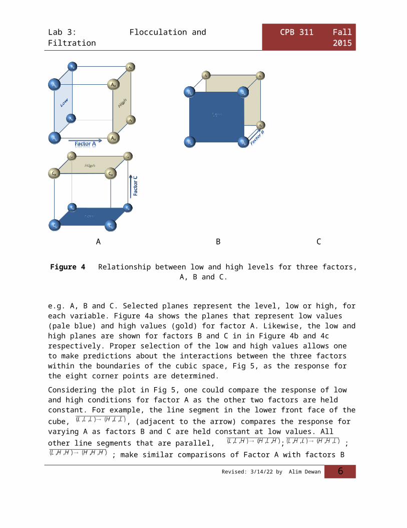
Figure 4 Relationship between low and high levels for three factors, A, B and C.
e.g. A, B and C. Selected planes represent the level, low or high, for each variable. Figure 4a shows the planes that represent low values (pale blue) and high values (gold) for factor A. Likewise, the low and high planes are shown for factors B and C in in Figure 4b and 4c respectively. Proper selection of the low and high values allows one to make predictions about the interactions between the three factors within the boundaries of the cubic space, Fig 5, as the response for the eight corner points are determined.
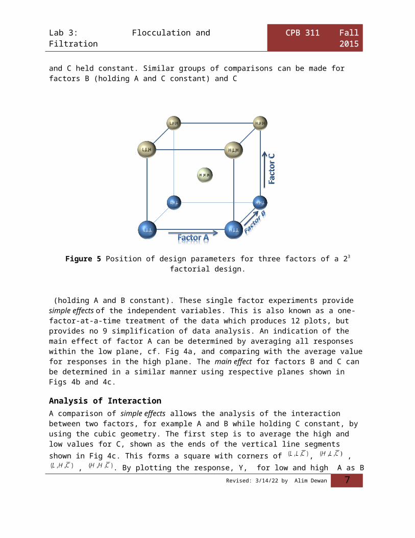
Considering the plot in Fig 5, one could compare the response of low and high conditions for factor A as the other two factors are held constant. For example, the line segment in the lower front face of the cube,
, (adjacent to the arrow) compares the response for varying A as factors B and C are
held constant at low values. All other line segments that are parallel, ;
; ; make similar comparisons of Factor A with factors B and C held constant. Similar groups of comparisons can be made for factors B (holding A and C constant) and C
Revised: 4/18/23 by Alim Dewan 4
Lab 3: Flocculation and Filtration CPB 311 Fall 2015
H,L,L
L,H,H
L,L,H
H,H,LL,H,L
L,L,L
H,H,H
M,M,M
H,L,H
Figure 5 Position of design parameters for three factors of a 23 factorial design.
(holding A and B constant). These single factor experiments provide simple effects of the independent variables. This is also known as a one-factor-at-a-time treatment of the data which produces 12 plots, but provides no 9 simplification of data analysis. An indication of the main effect of factor A can be deter-mined by averaging all responses within the low plane, cf. Fig 4a, and comparing with the average value for responses in the high plane. The main effect for factors B and C can be determined in a similar manner using respective planes shown in Figs 4b and 4c.
Analysis of InteractionA comparison of simple effects allows the analysis of the interaction between two factors, for example A and B while holding C constant, by using the cubic geometry. The first step is to average the high and low values for C, shown as the ends of the vertical line segments shown in Fig 4c. This forms a square with
corners of , , , . By plotting the response, Y, for low and high A as B is held low, and comparing this with the trend formed when B is high, one can determine the interaction be-tween A and B. There can be mild, strong or no interaction between variables. Figure 6 shows the rela-tionship between the trends for the three possible interactions that can occur. It should be obvious that the interaction is simply characterized by the change in slope, and one can use this to quantify the intensity of interaction, I, using the results from the equation:
One can see in Fig 6 that by forming a cross between the highest and lowest values of the two lines, and comparing the midpoints of the line segments, i.e. the average values, then the distance between the two indicates the intensity of interaction. By holding A or B constant and comparing the remaining factors, the interaction of other factors may be calculated similarly. Note that if no interaction exists between two variables, than it is best to compare the main effects, i.e. the average of two sets of four values, as dis-cussed in the preceding paragraph.
Revised: 4/18/23 by Alim Dewan 5
Lab 3: Flocculation and Filtration CPB 311 Fall 2015
Experimental Error
In experimentation, the replication of tests can be used to determine systematic and random error. The 23 design used in this experiment has eight corner points. An unbiased approach to determine the error would be to repeat each corner multiple times, which would greatly increase the testing effort. If only a selected number of points were chosen, then the results are biased by any underlying trends and interac-tions between factors that might exist. An unbiased solution to this is to conduct repetitive test on the cen-ter point of the cube. The center-point is defined as the average of the low and high values for each factor,
, as shown in Fig 3. By repeating the center point multiple times (usually more than 5 times for this experiment) a close approximation of the expected scatter of the response values for each point can be determined. Furthermore, if the center-point reps are distributed at intervals throughout the experi-ment, an increasing or decreasing trend is an indication of an underlying systematic error.
Low High
( , , )L L C
( , , )H L C
( , , )L H C
( , , )H H C
Factor B Low
Factor B High
No Interaction
Low High
( , , )L L C
( , , )H L C
( , , )L H C
( , , )H H C
Factor B Low
Factor B High
{Mild Interaction
Low High
( , , )L L C
( , , )H L C
( , , )L H C
( , , )H H C
Factor B Low
Factor B High }Strong Interaction
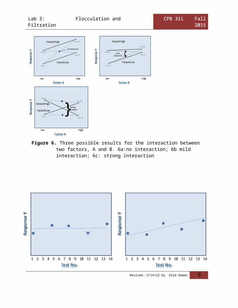
Figure 6. Three possible results for the interaction between two factors, A and B. 6a:no in-teraction; 6b mild interaction; 6c: strong interaction
Lab 3: Flocculation and Filtration CPB 311 Fall 2015
Figure 7. Plot of the repetition of center-point response measured at equal intervals during the experiment,
demonstrating 7a: random error only and; 7b: both random and systematic error.
Figure 7a shows the pattern of center point values plotted as a function of run order (time) which has ex-perimental scatter, or indeterminate error, but no systematic trend. Figure 7b illustrates both random error and a systematic increasing trend which has an adverse effect on the results. If a systematic error exists, one could easily apply a correction by using the equation of the line to calculate the fractional increase or decrease from the first point and use this multiplier to adjust each measured point during the experiment. Residual analysis of the data with respect to the systematic trend provides the random error for the experi-ment. Finally, in order prevent data from the effects of a systematic trend, experimental designs may also include randomization.
H,L,L
L,H,H
L,L,H
H,H,LL,H,L
L,L,L
H,H,H
H,L,H
M,M,M
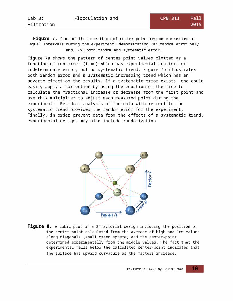
Figure 8. A cubic plot of a 23 factorial design including the position of the center point calculated from the av-erage of high and low values along diagonals (small green sphere) and the center-point determined experimentally from the middle values. The fact that the experimental falls below the calculated cen-ter-point indicates that the surface has upward curvature as the factors increase.
CurvatureWhen testing lower and upper bounding values (low and high) for factors, no information about the lin-earity of a trend can be inferred without intermediate points. If middle points were included on the design cube, an additional 12 tests would need to be performed, one at each midway point of each line segment. By measuring the center-point, the nature of each trend can be revealed. Departure from linearity, or cur-vature, can be detected by calculating the difference between the calculated middle point based on the av-erage of low and high boundary values with the measured response value, . If this value is posi-tive, then the measured point falls below the diagonal line and the relationship show an upward curvature, for example cf. Fig 8. This additional information can be quite useful for characterizing natural systems and for more improving predictive accuracy.
For additional reading on Factorial Design and the design of experiments please refer to the appendix.
Revised: 4/18/23 by Alim Dewan 7
Lab 3: Flocculation and Filtration CPB 311 Fall 2015
Preparation for Laboratory: In this laboratory exercise you will compare the three factors
Stirring Time after Polymer Addition low: 5 sec high: 1.5 min
You need to design an experimental plan that includes at least 5 middle points and randomizes the se-quence of tests according to the procedure outlined in the appendix. You should be able to present this ex-perimental plan before attempting to perform the lab on the day you are scheduled to.
You MUST read over the TAPPI standard method T-261, and be able to describe how to set up the DDJ for fractionation testing. You should also be able to describe the method you will use to test fines reten-tion and the testing of the flocculating agent.
You will need to indicate how much of the 0.01% polymer solution will be added to the DDJ assuming you have the proper volumes and solid contents of dilute suspension in the DDJ. READ T-261 very care-fully.
Safety: Always think SAFETY FIRST and take care of your fellow group members. Review the MSDS sheets for the polymer that may be found in the laboratory. You are required to use eye protection when performing this laboratory. At the dilute concentrations of the polymer solution, and the inert nature of the suspen-sion, latex gloves are optional. Wipe up all spills. Waste water from these experiments may be disposed of down the sink drain.
Be sure to clean up the apparatus, all glassware and the lab bench when you have completed the experi-ment.
Experimental:
MaterialsA dilute suspension of fibers and fine particles will be available. You need to determine the solid content of the suspension to the nearest 0.001% three replicates). The stock should be diluted to 0.5 wt% accord-ing to TAPPI method T-261. A dilute solution of polymeric retention aid will be provided at a known concentration.
Procedure
Please read the fractionation procedure of T-261 to know details of how to determine the fines content (D<75 µm) and read the Retention Procedure in T261 to understand how to characterize the three vari-ables, rpm, polymer concentration and mixing time. You will conduct the experiments following the pro-cedure adapted from the T-261 based on our laboratory need:
A. Determining total fibers and fines content: (duplicate the experiment)
Revised: 4/18/23 by Alim Dewan 8
Lab 3: Flocculation and Filtration CPB 311 Fall 2015
1. Take a known amount of sample in an aluminum pan. Make sure you know the initial
weight of the pan. Mark the pan with a sample number. Numbering should be done in way that you do not get confused with other group’s sample.
2. Dry the pan & sample overnight in an oven at 105oC. 3. (next day) Weight the pan & sample until you get a constant weight. You have to
weigh several times to make sure you have a constant weight, indicating no remaining moisture in the sample.
B. Determining the of fibers: (run in triplicate)1. Take about 500 ml sample in beaker. Weigh the beaker & sample. Make sure you
know the weight of the dry beaker.2. Prepare the Brit Jar with filter. Make sure to use the gasket. 3. Clamp the outlet tube of the jar. 4. Transfer the sample into the jar. 5. Stir the sample at 500 rpm for approximately 30 seconds. 6. Open the outlet tube after placing a beaker underneath; keep the stirrer running at the
same speed as step 5. Collect the filtrate in the beaker. You should see that the filtrate is cloudy. The clouds are formed due the fines (small size fibers and filler materials. Filler materials are CaCO3).
7. Clamp the outlet tube again.8. Add about 500 ml DI water into the jar, to wash the fines in the fiber. 9. Follow step 5 &6. You should see that the filtrate is less cloudy. 10. Repeat step 7-8-5-6 until you get clear filtrate, to make sure no fines remain in with
the fiber.4. Transfer the fibers from the Jar into an aluminum pan (Mark the pan with a sample
number. Numbering should be done in way that you do not get confused with samples from other groups. They will use same oven.) Make sure no remaining fibers in the jar and the filter. You may use small amount of DI water to wash out remaining fibers in the filter and wall of the jar, if necessary. Dry the pan & sample overnight in an oven at 105oC.
11. (next day) Weight the pan & sample until you get a constant weight. You have to weigh several times to make sure you have a constant weight, indicating no remaining moisture in the sample.
C. Determining the retention of the fines at different rpm, concentration of the reten-tion aid, and mixing time: (You have to run 8+5 = 13 set of experiments, ask one of our TAs to confirm your plan and the value of the factors)1. Take about 500 ml sample in beaker. Weigh the beaker & sample. You already know
the weight of the dry beaker.2. Prepare the Brit Jar with filter. Make sure to use the gasket. 3. Clamp the outlet tube of the jar. 4. Transfer the sample into the jar. 5. Stir the sample at a specific rpm (as you have planned for one of your 13 experi-
ments).
Revised: 4/18/23 by Alim Dewan 9
Lab 3: Flocculation and Filtration CPB 311 Fall 2015
6. Add specific amount of polymer while stirring. Start the timer.7. After adding polymer, stir for a specific period (mixing time). 8. Open the outlet tube after placing a beaker underneath; keep the stirrer running at the
same speed as step 7. Collect the filtrate in the beaker. 9. Transfer the fibers from the Jar into an aluminum pan. Make sure no remaining fibers
in the jar and the filter. You may use small amount of DI water to wash out remaining fibers in the filter and wall of the jar, if necessary.
10. Dry the pan & sample overnight in an oven at 105oC. 11. (next day) Weight the pan & sample until you get a constant weight. You have to
weigh several times to make sure you have a constant weight, indicating no remaining moisture in the sample.
Reporting: Each group should write a laboratory report for this lab exercise. It should contain all of the standard elements of a technical report. You should not replicate the experimental procedure from the TAPPI standard. Rather, give a brief description of what was done and cite the TAPPI standard for more de-tails. Your report should describe all aspects of your experiment that were unique, especially your ex-perimental plan and those aspects that deviated from the standards.
In the results section, report any anomalies, important observations, and of course the data that you collected. Conduct a thorough analysis of interactions, curvature and experimental error based on a 23
factorial design. Use plots and table where appropriate to explain results and defend your conclusion. A considerable amount of the lab grade is based on your ability to demonstrate the logical interpreta-tion of the data to show the relationship between the three parameters under examination.
Specifically, the report should include:
Analysis of systematic errors in the data (Run order plots, center point plots). Apply correc-tion if necessary.
A complete graphical analysis including cube plot, interaction plots and other plots as needed. Computation of factor effects and interactions Explanation of how factors were determined to be statistically significant or not Development of a mathematical model from these effects (an equation relating the three pa-
rameters) Computation of the predicted retention under a set of conditions different from those used in
your experiment. (Within the constraints of your experimental cube) Discussion should contain:
o A discussion of the internal consistency of the data, i.e. does it make any sense?
What points did not fall within expectations? How did you deal with these?o A mechanistic explanation of the main factor effects and also the interaction effects.