24
IFM – The Department of Physics, Chemistry and Biology Lab 71 in TFFM08 Fiber Optics NAME PERS. -NUMBER DATE APPROVED Rev Aug 10 Beyer
IFM – The Department of Physics, Chemistry and Biology
Lab 71 in TFFM08
Fiber Optics
NAME
PERS. -NUMBER
DATE
APPROVED
Rev Aug 10
Beyer

2
1 Introduction Optical fibers are a kind of waveguides, which are usually made of some kind of glass, can potentially be very long (hundreds of kilometers), and are – in contrast to other waveguides – fairly flexible. The most commonly used glass is silica (quartz glass, amorphous silicon diox-ide = SiO2), either in pure form or with some dopants. Silica is so widely used because of its outstanding properties, in particular its potential for extremely low propagation losses (real-ized with ultrapure material) and its amazingly high mechanical strength against pulling and even bending (provided that the surfaces are well prepared).
Most fibers used in laser optics have a core with a refractive index which is somewhat higher than that of the surrounding medium. The simplest case is that of a step-index fiber, where the refractive index is constant within the core and within the cladding.
Figure 1: Simple setup for launching light into a glass fiber (not to scale). A colli-mated laser beam is focused into the fiber core. The light propagates along the core and leaves the other fiber end as a diver-gent beam.
Figure 2: The fiber core and cladding are made of glass. A polymer jacket protects the fiber.
The index contrast between core and cladding determines the numerical aperture of the fiber (see below), and is typically small, so that fibers are weakly guiding. Light launched into the core is guided along the core, i.e., it propagates mainly in the core region, although the inten-sity distribution may extend somewhat beyond the core. Due to the guidance and the low propagation losses, the optical intensity can be maintained over long lengths of fiber.
Figure 1 shows a simple setup for launching light into a glass fiber (not to scale). A collimated laser beam is focused into the fiber core. The light propagates along the core and leaves the other fiber-end as a divergent beam. The fiber core and cladding are made of glass. A polymer jacket protects the fiber, see construction in Figure 2.1
1.1 Geometrical optics and fiber optics To understand what is occurring in these projects in fiber optics, it is necessary to under-stand some basic concepts of optics and physics. This section is intended to introduce these ideas for those who may not have studied the field and to review these ideas for those who have.
Light as an electromagnetic field The light waves, a combination of electric and magnetic fields, which can propagate through a vacuum, have as their most distinguishing features their wavelength and frequency of oscil-lation. The range of wavelengths for visible light is from about 400 nanometers (nm) to
1 http://www.rp-photonics.com/fibers.html

3
about 700 nm. In most of the work done in the field of fiber optics, the most useful sources of electromagnetic radiation emit just outside the visible in the near infrared with wavelengths in the vicinity of 800 to 1500 nm.
It can be difficult to follow what happens in an optical fiber system if the progress of light through the system is depicted in terms of the wave motion of the light. For the simplest cases it is easier to think of light traveling as a series of rays propagating through space. In a vac-uum, light travels at approximately 3 !108 m / s . In material media, such as air or water of glass, the speed is reduced. For air, the reduction is very small; for water, the reduction is about 25%; in glass, the reduction can vary from 30% to nearly 50%.
Light in materials In most cases, the results of the interaction of an electromagnetic wave with a material me-dium can be expressed in terms of a single number, the index of refraction of the medium. The refractive index is the ratio of the speed of light in a vacuum, c, to the speed of light in the medium, v,
n = c / v (1)
Since the speed of light in a medium is always less than it is in a vacuum, the refractive index is always greater than one. In air, the value is very close to one; in water, it is about 4/3 ( n = 1.33 ); in glasses, it varies from about 1.44 to about 1.9.
There are some qualifications to the simple picture presented here. First, the refractive index varies with the wavelength of the light. This is called wavelength dispersion. Second, not only can the medium slow down the light, but it can also absorb some of the light as it passes through.
In a homogeneous medium, that is, one in which the refractive index is constant in space, light travels in a straight line. Only when the light meets a variation or a discontinuity in the refractive index will the light rays be bent from their initial direction.
In the case of a variation in the refractive index within a material, the behavior of the light is governed by the way in which the index changes in space. For example, the air just above a road heated by the sun will be less dense than the air further from the road. Since the refrac-tive index increases with density, the refractive index of the air increases with height. This is called a refractive index gradient.
Figure 3: Geometry of reflection and refraction.
If the change in refractive index is not gradual, as in the case of the refractive index gradient, but is, instead, an abrupt change like that between glass and air, the direction of light is gov-erned by the Laws of Geometrical Optics. If the angle of incidence, !
i, of a ray is the angle be-
tween an incident ray and a line perpendicular to the interface at the point where the light ray strikes the interface (Figure 3), then:
4
1. Law of Reflection: The angle of reflection, !r, also measured with respect to the same
perpendicular, is equal to the angle of incidence:
!r= !
i (2)
2. Law of Refraction or Snell’s Law: The angle of the transmitted light is given by the relation:
ntsin!
t= n
isin!
i (3)
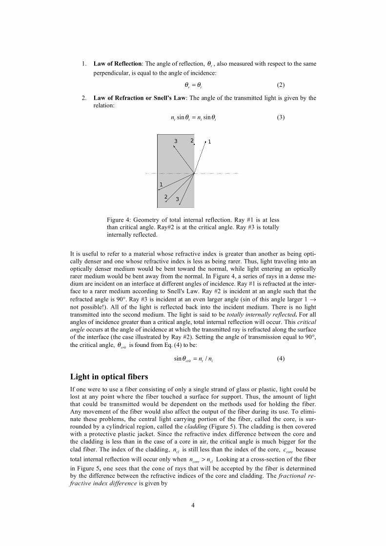
Figure 4: Geometry of total internal reflection. Ray #1 is at less than critical angle. Ray#2 is at the critical angle. Ray #3 is totally internally reflected.
It is useful to refer to a material whose refractive index is greater than another as being opti-cally denser and one whose refractive index is less as being rarer. Thus, light traveling into an optically denser medium would be bent toward the normal, while light entering an optically rarer medium would be bent away from the normal. In Figure 4, a series of rays in a dense me-dium are incident on an interface at different angles of incidence. Ray #1 is refracted at the inter-face to a rarer medium according to Snell's Law. Ray #2 is incident at an angle such that the refracted angle is 90°. Ray #3 is incident at an even larger angle (sin of this angle larger 1 → not possible!). All of the light is reflected back into the incident medium. There is no light transmitted into the second medium. The light is said to be totally internally reflected. For all angles of incidence greater than a critical angle, total internal reflection will occur. This critical angle occurs at the angle of incidence at which the transmitted ray is refracted along the surface of the interface (the case illustrated by Ray #2). Setting the angle of transmission equal to 90°, the critical angle, !
crit is found from Eq. (4) to be:
sin!crit
= nt/ n
i (4)
Light in optical fibers If one were to use a fiber consisting of only a single strand of glass or plastic, light could be lost at any point where the fiber touched a surface for support. Thus, the amount of light that could be transmitted would be dependent on the methods used for holding the fiber. Any movement of the fiber would also affect the output of the fiber during its use. To elimi-nate these problems, the central light carrying portion of the fiber, called the core, is sur-rounded by a cylindrical region, called the cladding (Figure 5). The cladding is then covered with a protective plastic jacket. Since the refractive index difference between the core and the cladding is less than in the case of a core in air, the critical angle is much bigger for the clad fiber. The index of the cladding, n
cl is still less than the index of the core, c
core because
total internal reflection will occur only when ncore
> ncl
Looking at a cross-section of the fiber in Figure 5, one sees that the cone of rays that will be accepted by the fiber is determined by the difference between the refractive indices of the core and cladding. The fractional re-fractive index difference is given by

5
! = (ncore
" ncl) / n
core (5)
Because the refractive index of the core is a constant and the index changes abruptly at the core-cladding interface, the type of fiber in Figure 5 is called a step-index fiber.
Figure 5: Step-index fiber. The refractive index profile is shown at the right. The geometry for derivation of the numerical aperture is given.
The definition of the critical angle can be used to find the size of the cone of light that will be accepted by an optical fiber with a fractional index difference, ! . In Figure 5 a ray is drawn that is incident on the core-cladding interface at the critical angle. If the cone angle is !
c, then by Snell's Law,
ntsin!
c= n
coresin!
t= n
coresin(90
!
"!crit)
= ncorecos!
crit
= ncore
1" sin2!crit
From Eq. (4):
ntsin!
c= n
core
2" n
cl
2 (6)
The numerical aperture, NA , is a measure of how much light can be collected by an optical system, whether it is an optical fiber or a microscope objective lens or a photo-graphic lens. It is the product of the refractive index of the incident medium and the sine of the maximum ray angle.
NA = nisin!
max (7)
In most cases, the light is incident from air and ni= 1 . In this case, the numerical aperture
of a step-index fiber is, from Eqs. (6) and (7),
NA = ncore
2! n
cl
2 (8)
When ! !1 , Eq. (7) can be approximated by
NA = (n
core+ n
cl)(n
core! n
cl)
= (2ncore)(n
core") = n
core2"
(9)
The condition in which ! !1 is referred to as the weakly-guiding approximation. The NA of a fiber will be measured in Project #1.
6
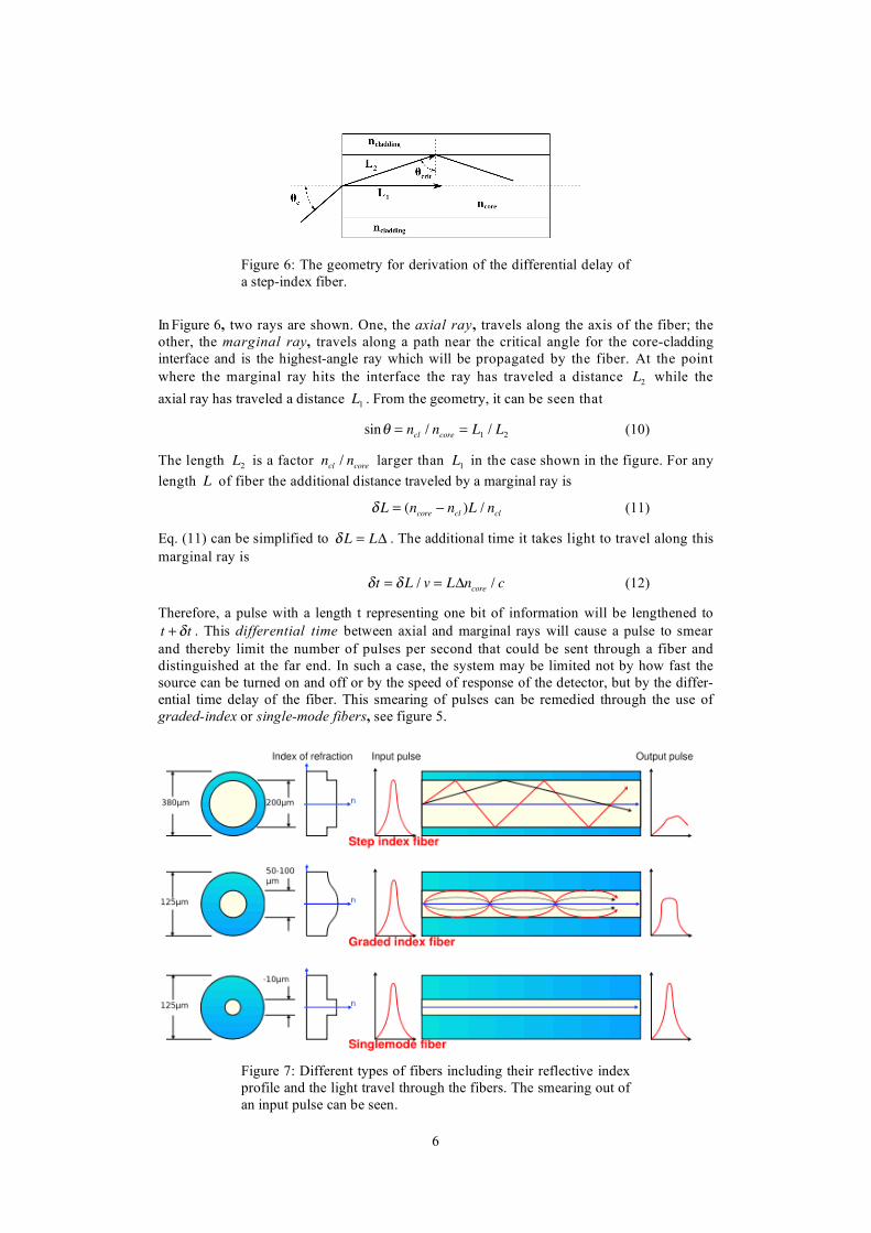
Figure 6: The geometry for derivation of the differential delay of a step-index fiber.
In Figure 6, two rays are shown. One, the axial ray, travels along the axis of the fiber; the other, the marginal ray, travels along a path near the critical angle for the core-cladding interface and is the highest-angle ray which will be propagated by the fiber. At the point where the marginal ray hits the interface the ray has traveled a distance L
2 while the
axial ray has traveled a distance L1. From the geometry, it can be seen that
sin! = ncl/ n
core= L
1/ L
2 (10)
The length L2
is a factor ncl/ n
core larger than L
1 in the case shown in the figure. For any
length L of fiber the additional distance traveled by a marginal ray is
!L = (ncore
" ncl)L / n
cl (11)
Eq. (11) can be simplified to !L = L" . The additional time it takes light to travel along this marginal ray is
!t = !L / v = L"ncore/ c (12)
Therefore, a pulse with a length t representing one bit of information will be lengthened to t + !t . This differential time between axial and marginal rays will cause a pulse to smear and thereby limit the number of pulses per second that could be sent through a fiber and distinguished at the far end. In such a case, the system may be limited not by how fast the source can be turned on and off or by the speed of response of the detector, but by the differ-ential time delay of the fiber. This smearing of pulses can be remedied through the use of graded-index or single-mode fibers, see figure 5.
Figure 7: Different types of fibers including their reflective index profile and the light travel through the fibers. The smearing out of an input pulse can be seen.
7
1.2 Wave optics and modes in optical fibers A fiber can support one or several (sometimes even many) guided modes, the intensity distri-butions of which are located at or immediately around the fiber core, although some of the intensity may propagate within the fiber cladding. In addition, there is a multitude of cladding modes, which are not restricted to the core region. The optical power in cladding modes is usually lost after some moderate distance of propagation, but can in some cases propagate over longer distances. Outside the cladding, there is typically a protective polymer coating, which gives the fiber improved mechanical strength and protection against moisture, and also determines the losses for cladding modes.1
Wave fields in a fiber The laws governing the propagation of light in optical fibers are Maxwell's equations. When information about the material constants, such as the refractive indices, and the boundary conditions for the cylindrical geometry of core and cladding is incorporated into the equa-tions, they may be combined to produce a wave equation that can be solved for those elec-tromagnetic field distributions that will propagate through the fiber. These allowed distributions of the electromagnetic field across the fiber are referred to as the modes. When the number of allowed modes becomes large, as is the case with large-diameter-core fibers, the ray picture we have used gives an adequate description of light propagation in fibers.
An important quantity in determining which modes of an electromagnetic field will be sup-ported by a fiber is a parameter called the characteristic waveguide parameter or the normalized wavenumber, or, simply, the V-number of the fiber. It is written as
V = k f !a !NA (13)
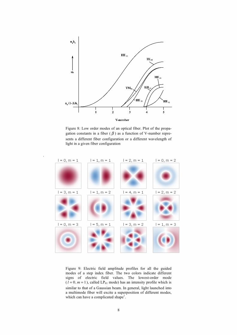
where k f is the free space wavenumber, 2! / " , a is the radius of the core, and NA . When the propagation constants ( ! ’s) of the fiber modes are plotted as a function of the V-number it is easy to determine the number of modes that can propagate in a particular fiber. In Error! Reference source not found., such a plot is given for some of the lowest order modes. The number of propagating modes is determined by the number of curves that cross a vertical line drawn at the V-number of the fiber. Note that for fibers with V < 2.405 , only a single modeHE
11 will propagate in the fiber. This is the single-mode
region. The wavelength at which V < 2.405 is called the cut-off wavelength, !c( all
higher-order modes are cut).
8
Figure 8: Low order modes of an optical fiber. Plot of the propa-gation constants in a fiber ( ! ) as a function of V-number repre-sents a different fiber configuration or a different wavelength of light in a given fiber configuration
.
Figure 9: Electric field amplitude profiles for all the guided modes of a step index fiber. The two colors indicate different signs of electric field values. The lowest-order mode ( l = 0, m = 1 ), called LP01 mode) has an intensity profile which is similar to that of a Gaussian beam. In general, light launched into a multimode fiber will excite a superposition of different modes, which can have a complicated shape1.

9
The LP modes are linearly polarized modes found from the exact theory of waveguides. The two subscripts describe the azimuthally or angular nodes, l and the radial nodes, m that occur in the electric field distribution of the mode.
Modes in multimode fibers The multimode fibers used for telecommunications may have a = 25 µm and NA = 0.2 or a = 50 µm and NA = 0.3 , so that for 633 nm light, the V-number will be about 50 or 150, respectively. This means that a large number of modes will be supported by the fiber. The amount of light carried by each mode will be determined by the input, or launch, conditions. For example, if the angular spread of the rays from the source is greater than the angular spread that can be accepted by the fiber (the NA of the input radiation is greater than the NA of the fiber) and the radius of the input beam is greater than the core radius of the fiber, then the fiber is said to be overfilled (Figure 10 (a)). That is, some of the light which the source will be putting into the fiber cannot be propagated by the fiber. Conversely, when the input beam NA is less than the fiber NA and the input beam radius is less than that of the fiber, the fiber is underfilled (Figure 10 (b)) and only low-order modes (low-angle rays in the ray picture) will be excited in the fiber. These two distributions will yield different measured attenuations, with the overfilled case having a higher loss than the underfilled case. In the ray picture, the higher-order rays will spend more of the time near the core-cladding interface and will have more of their evanescent field extending into the fiber clad-ding, resulting in higher attenuation. Also, if the fiber undergoes bending, the rays at high an-gles to the fiber axis may no longer satisfy the critical angle condition and not be totally internally reflected. Since power from these modes will radiate into the cladding and increase the attenuation, they are referred to as radiation modes. There is another class of modes called leaky modes. These modes have part of their electromagnetic energy distribution inside the core and part of their energy distribution in the cladding, but none of their en-ergy distribution is actually at the core-cladding interface. The energy in the core "leaks" into the cladding by a process known, from quantum mechanics, as tunneling. Leaky modes are not true guided modes, but may not be fully attenuated until the light has traveled long distances.
Figure 10: Launching conditions in a multimode optical fiber. (a) Overfilled. (b) Underfilled.
10
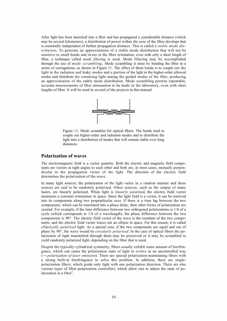
After light has been launched into a fiber and has propagated a considerable distance (which may be several kilometers), a distribution of power within the core of the fiber develops that is essentially independent of further propagation distance. This is called a stable mode dis-tribution. To generate an approximation of a stable mode distribution that will not be sensitive to small bends and twists in the fiber orientation, even with only a short length of fiber, a technique called mode filtering is used. Mode filtering may be accomplished through the use of mode scrambling . Mode scrambling is done by bending the fiber in a series of corrugations, as shown in Figure 11. The effect of these bends is to couple out the light in the radiation and leaky modes and a portion of the light in the higher-order allowed modes and distribute the remaining light among the guided modes of the fiber, producing an approximation of the stable mode distribution. Mode scrambling permits repeatable, accurate measurements of fiber attenuation to be made in the laboratory, even with short lengths of fiber. It will be used in several of the projects in this manual.
Figure 11: Mode scrambler for optical fibers. The bends tend to couple out higher-order and radiation modes and to distribute the light into a distribution of modes that will remain stable over long distances.
Polarization of waves The electromagnetic field is a vector quantity. Both the electric and magnetic field compo-nents are vectors at right angles to each other and both are, in most cases, mutually perpen-dicular to the propagation vector of the light. The direction of the electric field determines the polarization of the wave.
In many light sources, the polarization of the light varies in a random manner and these sources are said to be randomly polarized. Other sources, such as the output of many lasers, are linearly polarized. When light is linearly polarized, the electric field vector maintains a constant orientation in space. Since the light field is a vector, it can be resolved into its components along two perpendicular axes. If there is a time lag between the two components, which can be translated into a phase delay, then other forms of polarization are created. For example, if the time difference between two orthogonal polarizations is 1/4 of a cycle (which corresponds to 1/4 of a wavelength), the phase difference between the two components is 90°. The electric field vector of the wave is the resultant of the two compo-nents, and the electric field vector traces out an ellipse in space. For this reason, it is called elliptically polarized light. As a special case, if the two components are equal and out of phase by 90°, the wave would be circularly polarized. In the case of optical fibers the po-larization of light transmitted through them may be preserved or it may be scrambled to yield randomly polarized light, depending on the fiber that is used.
Despite the typically cylindrical symmetry, fibers usually exhibit some amount of birefrin-gence, which can cause the polarization state of light to evolve in an uncontrolled way (→ polarization of laser emission). There are special polarization-maintaining fibers with a strong built-in birefringence to solve this problem. In addition, there are single-polarization fibers, which guide only light with one polarization direction. There are also various types of fiber polarization controllers, which allow one to adjust the state of po-larization in a fiber1.
11
1.3 Transmitting power through optical fibers
Losses in fibers In all of the above discussion, it has been assumed that the light travels down the fiber with-out any losses beyond those from radiation and leaky modes and some higher-order modes that are coupled out into the cladding.
When light is transmitted through an absorbing medium, the irradiance falls exponentially with the distance of transmission. This relation, called Beer's Law, can be expressed as
I(z) = I(0)e!"z (14)
where I(z) is the irradiance at a distance z from a point z = 0 , and ! is the attenuation coefficient, expressed in units reciprocal to the units of z . In some fields of physics and chemistry, where absorption by a material has been carefully measured, the amount of absorption at a particular wavelength for a specific path length, such as 1 cm, can be used to measure the concentration of the absorbing material in a solution.
Although the absorption coefficient can be expressed in units of reciprocal length for expo-nential decay, in the field of fiber optics, as well as in most of the communications field, the absorption is expressed in units of dB/km (dB stand for decibels, tenths of a logarithmic unit). In this case, exponential decay is expressed using the base 10 instead of the base e ( = 2.7182818…) as
I(z) = I(0)10!"z/10 (15)
where z is in kilometers and ! is now expressed in decibels per kilometer kdB/km). Thus, a fiber of one kilometer length with an absorption coefficient of 10 dB/km permits I(z) / I(0) = 10
!(10"1/10)= 0.10 or 10% of the input power to be transmitted through the fiber.
Project #2 involves the measurement of the attenuation in an optical fiber.
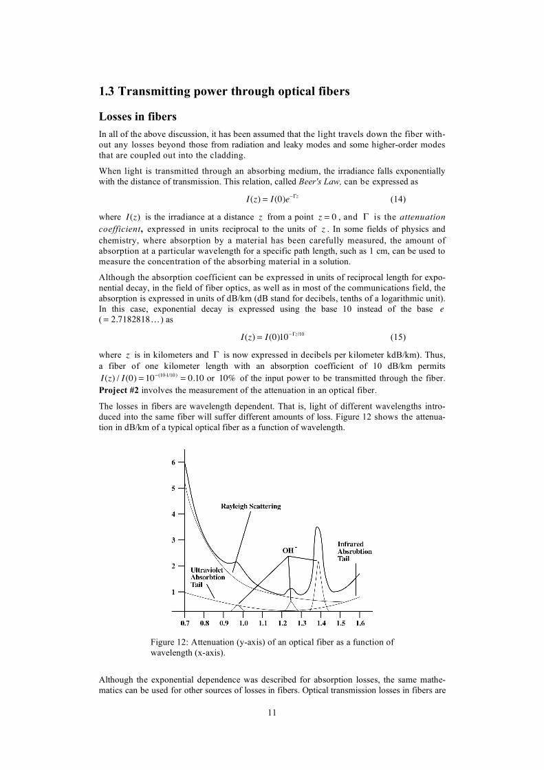
The losses in fibers are wavelength dependent. That is, light of different wavelengths intro-duced into the same fiber will suffer different amounts of loss. Figure 12 shows the attenua-tion in dB/km of a typical optical fiber as a function of wavelength.
Figure 12: Attenuation (y-axis) of an optical fiber as a function of wavelength (x-axis).
Although the exponential dependence was described for absorption losses, the same mathe-matics can be used for other sources of losses in fibers. Optical transmission losses in fibers are

12
due to several mechanisms. First, optical fibers are limited in the short wavelength region (to-ward the visible and ultraviolet) by absorption bands of the material and by scattering from inhomogeneities in the refractive index of the fiber. These inhomogeneities are due to ther-mal fluctuations when the fiber is in the molten state. As the fiber solidifies, these fluctuations cause refractive index variations on a scale smaller than the parabolic variation that is imposed upon graded-index fibers. Scattering off of the inhomogeneities is known as Rayleigh scat-tering and is proportional to !"4 , where ! is the wavelength of the light. (This same phe-nomenon is responsible for the color of the sky. The stronger scattering of light at shorter wavelengths gives the sky its blue color.)
In the long wavelength region, infrared absorption bands of the material limit the long wave-length end of the radiation spectrum to about 1600 nm. These two mechanisms are the ulti-mate limit for fiber losses. The highest quality fibers are sometimes characterized by how closely they approach the Rayleigh scattering limit, which is about 0.17 dB/km at 1550 nm.
At one time metal ions were the major source of absorption by impurities in optical fibers. It was the elimination of these ions that produced low-loss optical fibers. Today, the only impu-rity of consequence in optical fibers is water in the form of the hydroxyl ion (OH-), whose absorption bands at 950, 1250, and 1380 nm dominate the excess loss in today's fibers. They are evident in the absorption spectrum shown in Figure 12.
13
The following sections are as information to closer look on fiber fabrication, cleav-ing, and applications as well as the comparison to classical electric cables.
1.4 Fiber Fabrication Most optical fibers are fabricated by pulling from a so-called preform, which is a glass rod with a diameter of a few centimeters and roughly 1 m length. Along its axis, the preform con-tains a region with increased refractive index, which will form the core. When the preform is heated close to the melting point in a furnace (oven), a thin fiber with a diameter of typically 125 µm and a length of many kilometers can be pulled from the bottom of the preform. Before the fiber is wound up, it usually obtains a polymer coating for mechanical and chemical pro-tection.
The core of a fiber can be doped with laser-active ions, normally rare earth ions of erbium, neodymium, ytterbium, or thulium. When these ions are excited with suitable pump light, op-tical amplification occurs, which can be used in fiber lasers or amplifiers.
1.5 Polishing, Cleaving, and Splicing Clean and smoothly shaped fiber ends can be produced with polishing techniques. These can also be used to produce end faces that are not perpendicular to the fiber axis. With a tilt angle of the order of 10° (angle polishing), reflections from fiber ends can be effectively eliminated from the beam path, so that e.g. reflection-sensitive lasers are well protected. A much faster technique for preparing fiber ends is cleaving. Here, one typically pulls the fiber while scratching it from a side, e.g. with a vibrating diamond blade. This makes the fiber break with normally fairly smooth end faces – at least around the core region. By twisting the fiber during this process, angle cleaves can be fabricated, but the results are less reproducible than for pol-ishing techniques.
Fibers (particularly those made of silica) can also be spliced together. One may use the tech-nique of fusion splicing for making permanent fiber joints. A simpler technique is mechanical splicing, where the fiber ends are firmly held together by some mechanical means, but not fused. Here, however, the splice losses are typically higher, even when reduced with an index-matching gel between the surfaces.
In general, the handling of fiber ends is fairly delicate, compared with the handling of electri-cal connections. Apart from problems with dust, grease and the like, fiber ends are relatively sensitive and are easily scratched. Their handling often requires very expensive equipment (e.g. high-quality fusion splicers), particularly when reliable results are required under field conditions, i.e., in a comparatively dirty environment. On the other hand, a fair comparison with electrical cables has to take into account the much higher transmission capacity of a fi-ber.
1.6 Applications of Optical Fibers
There are many important applications of fiber optics. Some of the most important ones are: • Optical fiber communications utilize optical fibers mostly for long-range data trans-
mission, but sometimes also for short distances. Huge amounts of data can be quickly sent through a single fiber.
• Active fiber-optic devices contain some rare-earth-doped fiber. Fiber lasers can gen-erate laser light at various wavelengths, and fiber amplifiers can be used e.g. for boosting the optical power or amplifying some weak signals.
• Fiber-optic sensors can be used e.g. for distributed temperature and strain measure-ments in buildings, oil pipelines, and wings of airplanes.
14
• Passive fibers are useful for transporting light from some source to another point, e.g. for purposes like illumination, diode pumping of lasers and power over fiber. Also, they are used for connecting components in fiber-optic devices, such as interferome-ters and fiber lasers. They then play a similar role as electrical wires do in electronic devices.
Therefore, fiber optics has become a particularly important area within the technology of pho-tonics.
1.7 Comparison of Optical Fibers with Electric Cables In some technical areas, such as optical data transmission over long distances or between computer chips, optical fibers (or other waveguides) compete with electric cables. Compared with the latter, they have a number of pronounced advantages:
• Fiber cables are much less heavy than electric cables.
• The capacity of a fiber for optical data transmission is orders of magnitude higher than for any electric cable.
• The transmission losses of a fiber can be very low: well below 1 dB/km for the opti-mum wavelengths, which are around 1.5 µm.
• A large number of channels can be reamplified in a single fiber amplifier, if required for very large transmission distances.
• Optical data connections via fibers are comparatively hard to intercept and manipu-late, which gives additional security even without using encryption techniques. For very high security, quantum cryptography can be used.
• Fiber connections are immune to electromagnetic interference, problems with ground loops, and the like.
• Fibers do not introduce fire hazards or the risk of triggering explosive substances (unless a fiber carrying a high optical power breaks).
On the other hand, fibers also have their disadvantages: • Fiber connections are comparatively sensitive and difficult to handle, particularly
when single-mode fibers are used. Precise alignment and high cleanliness are re-quired. For such reasons, fiber connections are often only competitive if a high transmission bandwidth can be utilized.
• Fibers may not be bent very tightly, because this can cause high bend losses or even breakage. This can be a problem e.g. in the context of fiber-to-the-home technolo-gies.
• At least unprotected glass fibers are mechanically less robust than metallic wires.

15
2 Project #1: Handling fibers, numerical aper-ture
In this first project, you will learn how to prepare fiber ends for use in the laboratory. You will be able to observe the geometry of a fiber and you will measure the numerical aperture ( NA ) of a telecommunications-grade fiber and determine whether you work with a multimode or single mode fiber. Which modes can be observed?
The method which is presented for determining the NA of a fiber is especially illustrative of what is to be learned.
2.1 Fiber geometry An optical fiber is illustrated in Figure 13. It consists of a core, with refractive index n
core, of
circularly-symmetric cross section of radius a , and diameter 2a , and a cladding, with refractive index n
cl, which surrounds the core and has an outer diameter of d . Typical core diameters
range from 4-8 µm for single-mode fibers to 50-100 µm for multimode fibers used for com-munications to 200-1000 µm for large-core fibers used in power transmission applications. Communications-grade fibers will have d in the range of 125-150 µm , with some single-mode fibers as small as 80 µm . In high-quality communications fibers, both the core and the clad-ding are made of silica glass, with small amounts of impurities added to the core to slightly raise the index of refraction. There are also lower-quality fibers available which have a glass core surrounded by a plastic cladding, as well as some all-plastic fibers. The latter have very high attenuation coefficients and are used only in applications requiring short lengths of fiber.
Figure 13: Geometry of an optical fiber, showing core, cladding, and jacket.
Surrounding the fiber will generally be a protective jacket. This jacket may be made from a plastic and have an outside diameter of 500-1000 µm . However, the jacket may also be a very thin layer of varnish or acrylate material.
2.2 Fiber mechanical properties Before measuring the NA of a fiber, it will be necessary to prepare the ends of the fiber so, that light can be efficiently coupled in and out of the fiber. This is done by using a scribe-and-break technique to cleave the fiber. A carbide or diamond is used to start a small crack in the fiber, as illustrated in Figure 14. Evenly applied stress, applied by pulling the fiber, causes the

16
crack to propagate through the fiber and cleave it across a flat cross section of the fiber per-pendicular to the fiber axis.
Figure 14: Scribe-and-break technique of fiber cleaving. A car-bide blade makes a small scribe, or nick, in the fiber. The fiber is pulled to propagate the scribe through the fiber.
In theory, the breaking strength of glass fibers can be very large, up to about 5 GPa . However, because of inhomogeneities and flaws, fibers do not exhibit strengths anywhere near that value. Before being wound on a spool, a fiber is stretched over a pair of pulleys, which apply a fixed amount of strain (stretching per unit length). This process is called proof-testing. Typical commercial fibers may be proof-tested to about 345 MPa, which is equivalent to about a one pound load on a 125-µm OD fiber. When a crack is introduced, the strength is reduced even further in the neighborhood of the crack. Fracture occurs when the stress at the tip of the crack equals the theoretical breaking strength, even while the average stress in the body of the fiber is still very low1. The crack causes sequential fracturing of the atomic bonds only at the tip of the crack. This is the reason that a straight crack will yield a flat, cleaved, fiber face.
Optical fibers are required to have high strength while maintaining flexibility. Fiber fracture usually occurs at points of high strain when the fiber is bent. For a fiber of radius d / 2 , bent to a radius of curvature R , as shown in Figure 15, the surface strain on the fiber is the elongation of the fiber surface, (R + d / 2)! " R! , divided by the length of the arc, R! . The strain is, then, d / 2R . Although silica fibers have been prepared which can withstand strains of several per-cent, an upper strain limit of a fraction of 1% has been found to be necessary to guarantee fiber survival in a cable installed in the field2. If a strain limit of 0.5% is used as a reasonably conser-vative value, a 125-µm diameter fiber will be able to survive a bend radius of 1.25 cm.

17
Figure 15: Plot of the data taken in the measurement of the NA of the Newport F-MLD fiber.
2.3 Measuring numerical aperture A detailed derivation of the expression for the NA of a fiber was given in Section 1.1. Recall-ing Eq. (9), the NA of a fiber, in the weakly-guiding approximation, was found to be
NA = ncore
2! (16)
where ncore
is the refractive index of the core of a step-index fiber or the refractive index at the center of the core of a graded index fiber and ! is the fractional index difference,
! = (ncore
" ncl) / n
core (17)
As an example, a typical multimode communications fiber may have D = 0.01 , in which case the weakly-guiding approximation, which assumes ! !1 , is certainly justified. For silica-based fibers, n
core will be approximately 1.46. Using Eq. (16), these values of ! and n
core
give NA = 0.2 . This gives a value of 11.5° for the maximum incident angle in Figure 5 and a total cone angle of 23°. Values of NA range from about 0.1 for single-mode fibers to 0.2-0.3 for multimode communications fibers up to about 0.5 for large-core fibers.
The way in which light is launched into the fiber in the method used here to measure the fiber NA is shown in Figure 16.The light from the laser represents a wave front propagating in the z-direction. The width of the laser beam, ~1 mm, is much larger than the diameter of the fiber core, 100 µm in this case. In the neighborhood of the fiber core, the wave front of the laser light takes on the same value at all points having the same z, so we say that we have a plane wave prop agating parallel to the z-axis. When a plane wave is incident on the end face of a fiber, then we can be sure that all of the light launched into the fiber has the same incident angle, !c
, in Figure 16.
Figure 16: Geometry of a plane-wave launched of a laser beam into an optical fiber.

18
If the fiber end face is then rotated about the point O in Figure 16, we can then measure the amount of light accepted by the fiber as a function of the incident angle, !
c.
Figure 17 shows the light accepted by a Newport F-MLD fiber as a function of acceptance angle using the method just described. The point where the accepted radiation has fallen to a specified value is then used to define the maximum incident angle for the acceptance cone. The Electronic Industries Association uses the angle at which the accepted power has fallen to 5% of the peak accepted power as the definition of the experimentally determined NA 3. The 5% intensity points are chosen as a compromise to reduce requirements on the power level which has to be distinguished from background noise.4
Figure 17: Plot of the data taken in the measurement of the NA of the Newport F-MLD fiber.
Note that in Figure 17, the radiation levels were measured for both positive and negative rotations of the fiber and the NA was determined using one half of the full angle between the two 5%-intensity points. This eliminates any small errors resulting from not perfectly aligning !c= 0 to the plane wave laser beam. The NA obtained in this test case was 0.29, which
compares well with the manufacturer's specification of NA = 0.30 .
2.4 References 1. D. Kalish, et al., "Fiber Characterization-Mechanical", in Optical Fiber Communications, S. E. Miller and A. G. Chynoweth, eds., Academic Press (New York) 1979, p. 406
2. D. Gloge and W. B. Gardner, "Fiber Design Considerations", in Optical Fiber Communi-cations, S. E. Miller and A. G. Chynoweth, eds., Academic Press (New York) 1979, p. 152
3. EIA Standard RS_455-47, Section 4.3.2, EIA, Engineering Dept. (Washington D.C.) 1983
4. D. L. Franzen and E. M. Kim, "Interlaboratory measurement comparison to determine the radiation angle (NA) of graded-index optical fibers", Applied Optics 20, p. 1220 (1981)
19
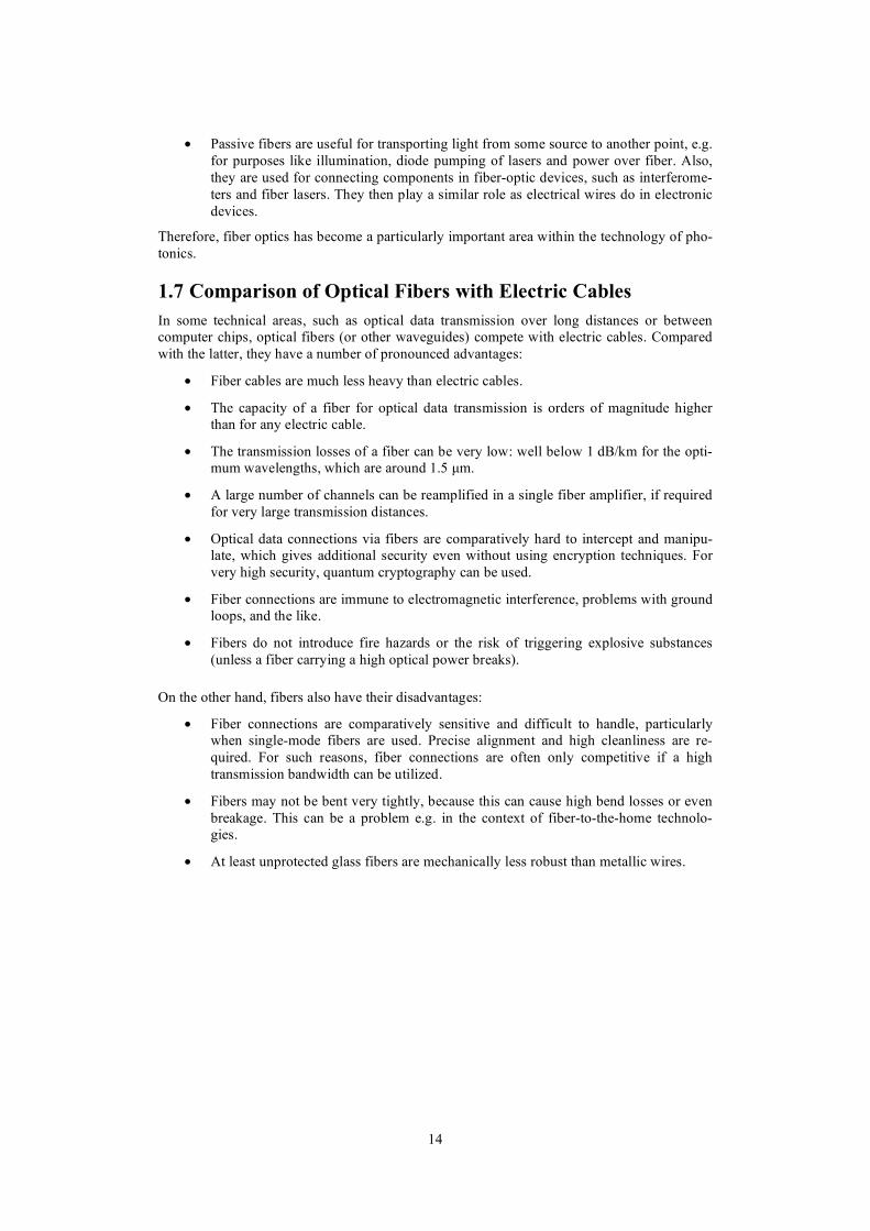
Figure 18: Cleaved fiber ends. (a) good cleave. (b) cracked fiber. (c) side view of a lip on the end of a fiber.
2.5 Instruction set
Preparing fiber ends 1. Use the Fiber Cleaver to cleave the stripped end of the fiber. The cleaver should be
placed on the top of the table with the blade pointing up. Draw the fiber over the blade with a light motion. Be sure that the fiber is normal to the blade. You should not attempt to cut the fiber with the cleaver. You are only starting a small nick which will propagate through the fiber when you pull it. Gently, but firmly, pull the fiber to cleave it.
2. Check the quality of the cleave by examining it under a high-power microscope. Carefully examine the end face of the fiber. The end face should appear flat and should be free of defects, as in Figure 18(a). However, chips or cracks which appear near the periphery of the fiber are acceptable if they do not extend into the central region of the fiber. Some poorly cleaved fiber ends are illustrated in Figure 18(b) and (c). The problems associated with the poor cleaves are discussed in Step 4.
3. If the inspection of the fiber end face in Step 3 does not show that the end face has been properly cleaved, you should consider the following common sources of error: There are two principal reasons for obtaining a bad cleave, 1) a poor scribe and 2) a non-uniform pull of the fiber. A scribe which is too deep may cause an irregular cleave and may cause multiple cracks to propagate through the fiber (Figure 18(b)). A scribe which is too shallow will be the same as no scribe at all and the fiber will break randomly. If the pull which propagates the crack through the fiber is not uni-form, and especially if it includes twisting of the fiber, irregularities may show up on the fiber end face or a lip may be formed on the end of the fiber, as in Figure 18(c). If the fiber end is cleaved at an angle, the fiber was probably scribed at an angle other than 900 across the fiber axis, although this, too, can be caused by a non-uniform pull of the fiber.

20
Measuring numerical aperture 1. Extend the tip of the fiber and orient the Positioner so that the fiber tip is at the cen-
ter of rotation of the stage. This is a critical step if an accurate value for the fiber NA is to be obtained.
2. Check the alignment of your light-launching system by making sure that the tip of the fiber remains at the center of the laser beam as the stage is rotated. This set up achieves plane-wave launching into the end of your fiber.
3. Mount the far end of the fiber in a Fiber Holder (taken from the Fiber Positioner) and the Fiber Positioner. You can get a quick approximate measure of the fiber's NA with a 3! 5 card placed a distance, L , away from the laser in a darkened room, as shown in Figure 19. Measure the width, w , on the card of the spot out of the fiber and the distance, L , from the fiber to the card. The NA of the fiber is approximately sin
!1(w / (2L)) . This is a quick method which is used when only an approximate
measurement of a fiber's NA is needed. 4. Mount the detector head of the Power Meter so that the output beam from the fiber is
incident on the detector head. You will find this to be necessary, because the power lev-els obtained in plane-wave launching are low. Block the laser beam and note the power measured by the power meter. This determines the stray light seen by the meter. You will need to subtract this amount from all of your data.
5. Measure the power accepted by the fiber as a function of the incident angle of the plane-wave laser beam. Use both positive and negative rotation directions to com-pensate for any remaining error in laser-fiber alignment.
6. Plot the power received by the detector as a function of the sine of the acceptance an-gle. Semi-log paper is recommended. Measure the full width of the curve at the points where the received power is at 5% of the maximum intensity. The half-width at this intensity is the experimentally determined numerical aperture of the fiber. Com-pare your results with the results of Step 6 and Figure 17.
7. Determine the modes of the fiber (Figure 7) and compare the light pattern of a single and a multimode fiber using the HeNe-laser as light source (HINT: take care about the wavelength when judging!)
Figure 19: Approximate measure of the NA of a fiber.

21
3 Project #2: Fiber attenuation In this exercise, you will measure one of the most important fiber parameters, the attenuation per unit length, of a multimode communications-grade optical fiber. The technique demon-strated here is called the “cutback method” and is generally used for this measure-ment.
You will also be introduced to the way that the conditions under which light is launched into the fiber can affect this measurement. You learn about mode scrambling and how to generate a desirable distribution of light in the fiber.
3.1 Measurement of optical fiber attenuation Section 1.3 contained a detailed description of the loss mechanisms in optical fibers. An expression for the amount of optical power which still remains in a fiber after it has propa-gated a distance, z , was given in Eq. (15) as
I(z) = I(0)10!"z/10 (18)
The length of the fiber, z , is given in kilometers, and the attenuation coefficient, ! , is given in decibels per kilometer (dB/km).
Because the designers of fiber optic systems need to know how much light will remain in a fiber after propagating a given distance, one of the most important specifications of an op-tical fiber is the fiber's attenuation. In principle, the fiber attenuation is the easiest of all fiber measurements to make. The method which is generally used is called the “cut-back method:” All that is required is to launch power from a source into a long length of fiber, measure the power at the far end of the fiber using a detector with a linear response, and then, after cutting off a length of the fiber, measure the power transmitted by the shorter length. The reason for leaving a short length of fiber at the input end of the system is to make sure that the loss that is measured is due solely to the loss of the fiber and not to loss which occurs when the light source is coupled to the fiber. Figure 20 shows a schematic illustration of the measurement system.
Figure 20: Schematic of laboratory set-up for cutback method of determining fiber attenuation.
The transmission through the fiber is written as
T = Pf / Pi (19)
where we have substituted Pi (initial power) and Pf , (final power) for I(0) and I(z) , respec-
tively. A logarithmic result for the loss in decibels (dB), is given by
L dB[ ] = !10 log(Pf / Pi ) (20)
The minus sign causes the loss to be expressed as a positive number. This allows losses to be summed and then subtracted from an initial power when it is also expressed logarithmi-cally. (In working with fiber optics, you will often find powers expressed in dBm, which
22
means “dB with respect to 1 mW of optical power.” Thus, e.g., 0 dBm = 1 mW, 3 dBm = 2 mW, and -10 dBm = 100 µW. Note that when losses in dB are subtracted from powers in dBm, the result is in dBm. For example, an initial power of t 3 dBm minus a loss of 3 dB re-sults in a final power of 0 dBm. This is a shorthand way of saying “An initial power of 2 mW with a 50% loss results in a final power of 1 mW”)
The attenuation coefficient, r , in dB/km is found by dividing the loss, L , by the length of the fiber, z . The attenuation coefficient is then given by
! dB/km[ ] = (1 / z)("10 log(Pf / Pi )) (21)
The total attenuation can then be found by multiplying plying the attenuation coefficient by the fiber length, giving a logarithmic result, in decibels (dB), for the fiber loss.
3.2 Practical problems The cutback method works well for high-loss fibers, with ! on the order of 10 to 100 dB/km. However, meaningful measurements on low-loss fibers are more difficult. The highest-quality fibers will have losses which are on the order of I dB/km or less, so that cutting a full 1 km from the fiber will result in a transmitted power decrease of less than 20%, put-ting greater demands on the measurement system's resolution and accuracy.
There is also an uncertainty due to the fact that the measured loss will depend on the characteristics of the way in which light is launched into the fiber. When a fiber is over-filled, many high-order and radiation modes are launched. These modes are more highly attenuated than are low-order modes. When a fiber is underfilled, mostly low-order modes are launched and lower losses occur.
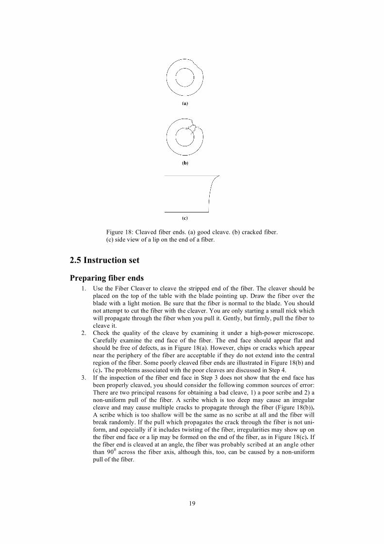
The solution to this problem is to attempt to generate what is known as the stable mode distribution as quickly as possible after launching. Figure 21 compares the transmission characteristics of the stable distribution with those of the overfilled and underfilled launch conditions. The stable mode distribution may be achieved, even in a short length of fiber, by using mode scrambling to induce coupling between the modes shortly after the light is launched.
Figure 21: Comparison of attenuation characteristics of various launch conditions.
23
Mode scrambling generates an approximation of a stable distribution immediately after launch and allows repeatable measurements, which approximate those that would be found in the field, to be made in the laboratory. Figure 21 compares the optical power in a fiber as a function of propagation distance for the three types of launch conditions: overfilled, under-filled, and stable distribution. The slope of the curve at large distances is equal to the attenuation coefficient. It is the fact that the mode scrambling generates a stable distribu-tion immediately after the source that allows a short cutback length to be used in the cutback method of measuring attenuation.
3.3 Reference 1. D. Marcuse, Principles of Optical Fiber Measurements, Academic Press (New York) 1981, p. 226-236
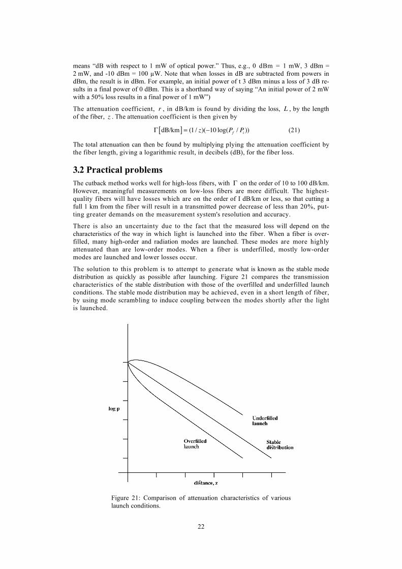
Figure 22: Coupling of HeNe laser light into a fiber using the Fiber Coupler.
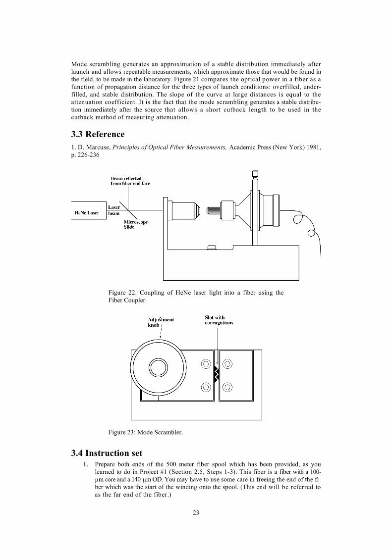
Figure 23: Mode Scrambler.
3.4 Instruction set 1. Prepare both ends of the 500 meter fiber spool which has been provided, as you
learned to do in Project #1 (Section 2.5, Steps 1-3). This fiber is a fiber with a 100-µm core and a 140-µm OD. You may have to use some care in freeing the end of the fi-ber which was the start of the winding onto the spool. (This end will be referred to as the far end of the fiber.)
24
2. Place the cleaved far end of the fiber in an holder which has been removed from Posi-tioner and insert this into the post-mounted . Also, post mount the detector head of the power meter. Align the detector head with the fiber end so that you will be able to measure the output power.
3. The use of the Fiber Coupler to couple light from a HeNe laser into a fiber is illus-trated in Figure 22. Align the coupler and the HeNe laser so that the laser beam shines along the axis of the Fiber Coupler. Place the cleaved front end of the fiber into the fiber chuck and insert this into the coupler. Carefully align the fiber to maximize the light launched into the fiber, using the power meter to monitor the launched power.
4. Position the Mode Scrambler at a convenient place near the launch end of the fiber. 5. Rotate the knob of the Mode Scrambler counter-clockwise to fully separate the two
corrugated surfaces. The Mode Scrambler is illustrated in Figure 23. Place the fiber between the two corrugated surfaces of the Mode Scrambler. Leave the fiber jacket on to protect the fragile glass fiber. Rotate the knob clockwise until the corrugated surfaces just contact the fiber. Examine the far-field distribution of the output of the fiber. Rotate the knob further clockwise and notice the changes in the distribution as the amount of bending of the fiber is changed. Since a narrow, collimated HeNe beam is being used to launch light into the fiber, the original launched dis-tribution will be underfilled. When the distribution of the output just fills the NA of the fiber, an approximation of the stable distribution has been achieved. Do not add any more bending than is necessary to accomplish this, since that will re-sult in excess loss. This launching and mode scrambling set-up should not be changed again during the remainder of the exercise.
6. Measure the power out of the far end of the fiber. Note the exact length of the fiber. It will be part of the information on the label of the spool.
7. Break off the fiber ~2 meters after the mode scrambler (see Figure 20) from the launching set-up. (Be sure to note on the spool how much fiber you have removed, so that other people using the same spool in the future will be able to obtain accurate results.) Cleave the broken end of the fiber and measure the output from the cutback segment.
8. Calculate the fiber attenuation, using Eq. (21), and compare this with the attenuation written in the fiber specification on the spool. Your value is probably somewhat higher than the specification. Why? (HINT: Go back and look at Figure 12. Remember, the HeNe laser operates at a wavelength of 633 nm.)


