QMP 7.1 D/F
Channabasaveshwara Institute of Technology (An ISO 9001:2008 Certified Institution)
NH 206 (B.H. Road), Gubbi, Tumkur – 572 216. Karnataka.
Department of Mechanical Engineering
LAB MANUAL
(2015-2016)
COMPUTER AIDED MODELING AND ANALYSIS LAB
(CAMA LAB-10MEL68)
VI SEMESTER
NAME: __________________________________________
USN : __________________________________________
BATCH: _______________SECTION:_________________
CONTENTS
SL.
NO Title
PPAGE
NO.
1. Performing a Typical ANSYS Analysis 1
2. General Steps 4
3. Bars of Constant Cross-section Area 5
4. Bars of Tapered Cross section Area 7
5. Stepped Bar 10
6. Trusses 12
7. Simply Supported Beam 18
8. Simply Supported Beam with Uniformly
varying load 21
9. Simply Supported Beam with Uniformly
distributed load 24
10. Beam with moment and overhung 27
11. Cantilever Beam 30
12. Beam with angular loads, one end hinged and
at other end roller support 32
13. Stress analysis of a rectangular plate with a
circular hole 35
14. Corner angle bracket 37
15. Thermal analysis 39
16. Modal Analysis of Cantilever beam for
natural frequency determination 52
17. Fixed- fixed beam subjected to forcing
function 54
18. Bar subjected to forcing function 56
19. Additional problems
20. Viva questions
ii
INDEX PAGE
Note:
• If the student fails to attend the regular lab, the experiment
has to be completed in the same week. Then the
manual/observation and record will be evaluated for 50% of
maximum marks.
Date Sl.No
Name of the Experiment
Conduction Repetition Submission of
Record Manual Marks
(Max . 25)
Record Marks
(Max. 10)
Signature
(Student)
Signature
(Faculty)
Average
QMP 7.1 D/D
Channabasaveshwara Institute of Technology (An ISO 9001:2008 Certified Institution)
NH 206 (B.H. Road), Gubbi, Tumkur – 572 216. Karnataka.
DEPARTMENT OF MECHANICAL ENGINEERING
SYLLABUS
COMPUTER AIDED MODELING AND ANALYSIS LAB
Sub Code: 10MEL68 IA Marks : 25
Hrs/ Week: 03 Exam Hours: 03
Total Hrs. 42 Exam Marks: 50
PART - A
Study of a FEA package and modeling stress analysis of
a. Bars of constant cross section area, tapered cross section area and stepped bar 6 Hours
b. Trusses – (Minimum 2 exercises) 3 Hours
c. Beams – Simply supported, cantilever, beams with UDL, beams with varying load etc
(Minimum 6 exercises) 12 Hours
PART - B
a) Stress analysis of a rectangular plate with a circular hole. 3 Hours
b) Thermal Analysis – 1D & 2D problem with conduction and convection boundary
conditions. (Minimum 4 exercises) 9 Hours
c) Dynamic Analysis
1) Fixed – fixed beam for natural frequency determination
2) Bar subjected to forcing function
3) Fixed – fixed beam subjected to forcing function 9 Hours
REFERENCE BOOKS:
1. A first course in the Finite element method, Daryl L Logan, Thomason, Third Edition
2. Fundaments of FEM, Hutton – McGraw Hill, 2004
3. Finite Element Analysis, George R. Buchanan, Schaum Series
Scheme for Examination:
One Question from Part A - 20 Marks (05 Write up +15)
One Question from Part B - 20 Marks (05 Write up +15)
Viva-Voce - 10 Marks
COMPUTER AIDED ANALYSIS AND MODELING LAB [10 MEL68]
DEPARTMENT OF MECHANICAL ENGINEERING, C.I.T, GUBBI 1
Performing a Typical ANSYS Analysis
The ANSYS program has many finite element analysis capabilities, ranging from a simple,
linear, static analysis to a complex, nonlinear, transient dynamic analysis. The analysis guide
manuals in the ANSYS documentation set describe specific procedures for performing
analyses for different engineering disciplines.
A typical ANSYS analysis has three distinct steps:
� Build the model.
� Apply loads and obtain the solution.
� Review the results.
Building a Model
Building a finite element model requires more of an ANSYS user's time than any other part
of the analysis. First, you specify a job name and analysis title. Then, you use the PREP7
preprocessor to define the element types, element real constants, material properties, and the
model geometry.
Specifying a Job name and Analysis Title
This task is not required for an analysis, but is recommended.
Defining the Job name
The job name is a name that identifies the ANSYS job. When you define a job name for an
analysis, the job name becomes the first part of the name of all files the analysis creates. (The
extension or suffix for these files' names is a file identifier such as .DB.) By using a job name
for each analysis, you insure that no files are overwritten. If you do not specify a job name,
all files receive the name FILE or file, depending on the operating system.
Command(s): /FILNAME
GUI: Utility Menu>File>Change Job name
Defining Element Types
The ANSYS element library contains more than 100 different element types. Each element
type has a unique number and a prefix that identifies the element category: BEAM4,
PLANE77, SOLID96, etc. The following element categories are available
COMPUTER AIDED ANALYSIS AND MODELING LAB [10 MEL68]
DEPARTMENT OF MECHANICAL ENGINEERING, C.I.T, GUBBI 2
The element type determines, among other things:
� The degree-of-freedom set (which in turn implies the discipline-structural, thermal,
magnetic, electric, quadrilateral, brick, etc.)
� Whether the element lies in two-dimensional or three-dimensional space.
For example, BEAM4, has six structural degrees of freedom (UX, UY, UZ, ROTX, ROTY,
ROTZ), is a line element, and can be modeled in 3-D space. PLANE77 has a thermal degree
of freedom (TEMP), is an eight-node quadrilateral element, and can be modeled only in 2-D
space.
Defining Element Real Constants
Element real constants are properties that depend on the element type, such as cross-sectional
properties of a beam element. For example, real constants for BEAM3, the 2-D beam
element, are area (AREA), moment of inertia (IZZ), height (HEIGHT), shear deflection
constant (SHEARZ), initial strain (ISTRN), and added mass per unit length (ADDMAS). Not
all element types require real constants, and different elements of the same type may have
different real constant values.
As with element types, each set of real constants has a reference number, and the table of
reference number versus real constant set is called the real constant table. While defining the
elements, you point to the appropriate real constant reference number using the REAL
command
(Main Menu> Preprocessor>Create>Elements>Elem Attributes).
Defining Material Properties
Most element types require material properties. Depending on the application, material
properties may be:
� Linear or nonlinear
� Isotropic, orthotropic, or anisotropic
� Constant temperature or temperature-dependent.
As with element types and real constants, each set of material properties has a material
reference number. The table of material reference numbers versus material property sets is
called the material table. Within one analysis, you may have multiple material property sets
(to correspond with multiple materials used in the model). ANSYS identifies each set with a
unique reference number.
COMPUTER AIDED ANALYSIS AND MODELING LAB [10 MEL68]
DEPARTMENT OF MECHANICAL ENGINEERING, C.I.T, GUBBI 3
Main Menu > Preprocessor> Material Props > Material Models.
Creating the Model Geometry
Once you have defined material properties, the next step in an analysis is generating a finite
element model-nodes and elements-that adequately describes the model geometry.
There are two methods to create the finite element model: solid modeling and direct
generation.
With solid modeling, you describe the geometric shape of your model, and then instruct the
ANSYS program to automatically mesh the geometry with nodes and elements. You can
control the size and shape of the elements that the program creates. With direct generation,
you "manually" define the location of each node and the connectivity of each element.
Several convenience operations, such as copying patterns of existing nodes and elements,
symmetry reflection, etc. are available.
Apply Loads and Obtain the Solution
In this step, you use the SOLUTION processor to define the analysis type and analysis
options, apply loads, specify load step options, and initiate the finite element solution. You
also can apply loads using the PREP7 preprocessor.
Applying Loads
The word loads as used in this manual includes boundary conditions (constraints, supports, or
boundary field specifications) as well as other externally and internally applied loads. Loads
in the ANSYS program are divided into six categories:
� DOF Constraints
� Forces
� Surface Loads
� Body Loads
� Inertia Loads
� Coupled-field Loads
You can apply most of these loads either on the solid model (keypoints, lines, and areas) or
the finite element model (nodes and elements).
Two important load-related terms you need to know are load step and substep. A load step is
simply a configuration of loads for which you obtain a solution. In a structural analysis, for
example, you may apply wind loads in one load step and gravity in a second load step. Load
steps are also useful in dividing a transient load history curve into several segments.
COMPUTER AIDED ANALYSIS AND MODELING LAB [10 MEL68]
DEPARTMENT OF MECHANICAL ENGINEERING, C.I.T, GUBBI 4
PART-A
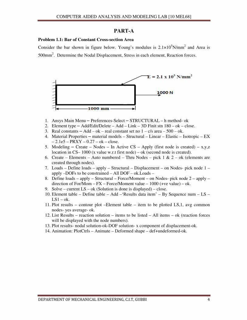
Problem 1.1: Bar of Constant Cross-section Area
Consider the bar shown in figure below. Young’s modulus is 2.1×10⁵N/mm
2 and Area is
500mm2. Determine the Nodal Displacement, Stress in each element, Reaction forces.
1. Ansys Main Menu – Preferences-Select – STRUCTURAL – h method- ok
2. Element type – Add/Edit/Delete – Add – Link – 3D Finit stn 180 – ok – close.
3. Real constants – Add – ok – real constant set no 1 – c/s area – 500 – ok.
4. Material Properties – material models – Structural – Linear – Elastic – Isotropic – EX
– 2.1e5 – PRXY – 0.27 – ok – close.
5. Modeling – Create – Nodes – In Active CS – Apply (first node is created) – x,y,z
location in CS– 1000 (x value w.r.t first node) – ok (second node is created).
6. Create – Elements – Auto numbered – Thru Nodes – pick 1 & 2 – ok (elements are
created through nodes).
7. Loads – Define loads – apply – Structural – Displacement – on Nodes- pick node 1 –
apply –DOFs to be constrained – All DOF – ok.Loads –
8. Define loads – apply – Structural – Force/Moment – on Nodes- pick node 2 – apply –
direction of For/Mom – FX – Force/Moment value – 1000 (+ve value) – ok.
9. Solve – current LS – ok (Solution is done is displayed) – close.
10. Element table – Define table – Add –‘Results data item’ – By Sequence num – LS –
LS1 – ok.
11. Plot results – contour plot –Element table – item to be plotted LS,1, avg common
nodes- yes average- ok.
12. List Results – reaction solution – items to be listed – All items – ok (reaction forces
will be displayed with the node numbers).
13. Plot results- nodal solution-ok-DOF solution- x component of displacement-ok.
14. Animation: PlotCtrls – Animate – Deformed shape – def+undeformed-ok.
COMPUTER AIDED ANALYSIS AND MODELING LAB [10 MEL68]
DEPARTMENT OF MECHANICAL ENGINEERING, C.I.T, GUBBI 5
RESULT:
Analytical approach:
Calculation:
Displacement: ______________________
Stress: ____________________________
Reaction force: _____________________
Ansys results:
Ansys Theoretical
Deformation
Stress
Reaction
COMPUTER AIDED ANALYSIS AND MODELING LAB [10 MEL68]
DEPARTMENT OF MECHANICAL ENGINEERING, C.I.T, GUBBI 6
Problem 1.2: Bars of Tapered Cross section Area
Consider the Tapered bar shown in figure below. Determine the Nodal Displacement,
Stress in each element, Reaction forces
E = 2 x 10⁵ N/mm
2, Area at root, A1 = 1000 mm
2, Area at the end, A2 = 500 mm
2.
Solution: The tapered bar is modified into 2 elements as shown below with modified area of
cross section.
(A1 + A2)/2= (1000+500)/2=750 mm2
A1 = (1000+750)/2= 875 mm2
A2= (500+750)/2=625 mm2
L1 = 187.5 mm & L2 = 187.5 mm
1. Ansys Main Menu – Preferences-Select – STRUCTURAL- h method– ok
2. Element type – Add/Edit/Delete – Add – link, 3D Finit stn 180 – ok- close.
3. Real constants – Add – ok – real constant set no – 1 – cross-sectional AREA1 – 875 –
apply-ok
4. Add – ok – real constant set no – 2 – cross-sectional AREA 2 – 625-ok
5. Material Properties – material models – Structural – Linear – Elastic – Isotropic – EX
– 2e5 –PRXY – 0.3 – ok – close.
6. Modeling – Create – keypoints– In Active CS, =0, Y=0 – Apply (first key point is
created) – location in active CS, X= 187.5, Y=0, apply (second key point is created) -
location in active CS X=375, Y=0(third key point is created) -ok.
7. Modeling-Create – lines-straight lines-pick key points 1 & 2-ok- pick key points 2 &
3-ok
8. Meshing-mesh attributes-picked lines (pick the lines)-ok-material no= 1, real
constants set no = 1, element type no =1, link 1, element section= none defined-pick
the other line-ok-material number 2-define material id 2- real constants set no = 2,
element type no =2-element section= none defined-ok.
COMPUTER AIDED ANALYSIS AND MODELING LAB [10 MEL68]
DEPARTMENT OF MECHANICAL ENGINEERING, C.I.T, GUBBI 7
9. Meshing-size controls-manual size-lines-all lines- no of element divisions=10(yes)-ok
10. Meshing-mesh tool-mesh-pick the lines-ok (the color changes to light blue)
11. Loads – Define loads – apply – Structural – Displacement – on key points- pick key
point 1 – apply –DOFs to be constrained – ALL DOF, displacement value=0 – ok.
12. Loads – Define loads – apply – Structural – Force/Moment – on key points- pick last
key point – apply – direction of For/Mom – FX – Force/Moment value – 1000 (+ve
value) – ok.
13. Solve – current LS – ok (Solution is done is displayed) – close.
14. Element table – Define table – Add –‘Results data item’ – By Sequence num – LS –
LS1 – ok.
15. Plot results – contour plot –Element table – item to be plotted LS,1, avg common
nodes- yes average- ok.
16. List Results – reaction solution – items to be listed – All items – ok (reaction forces
will be displayed with the node numbers).
17. Plot results- nodal solution-ok-DOF solution- x component of displacement-ok.
18. Animation: PlotCtrls – Animate – Deformed shape – def+undeformed-ok.
RESULT:
Analytical approach:
Calculation:
COMPUTER AIDED ANALYSIS AND MODELING LAB [10 MEL68]
DEPARTMENT OF MECHANICAL ENGINEERING, C.I.T, GUBBI 8
Displacement: ______________________
Stress: ____________________________
Reaction force: _____________________
Ansys results:
Ansys Theoretical
Deformation
Stress
Reaction
COMPUTER AIDED ANALYSIS AND MODELING LAB [10 MEL68]
DEPARTMENT OF MECHANICAL ENGINEERING, C.I.T, GUBBI 9
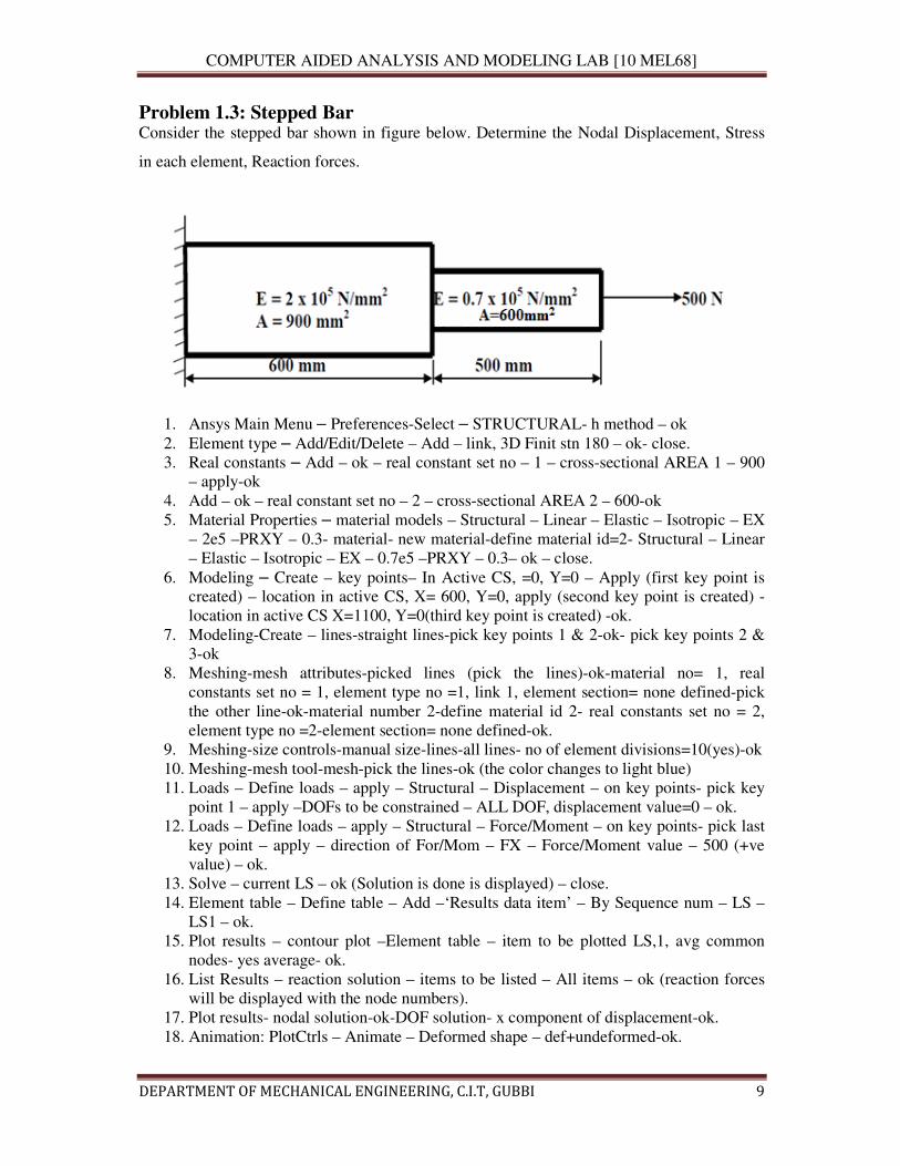
Problem 1.3: Stepped Bar Consider the stepped bar shown in figure below. Determine the Nodal Displacement, Stress
in each element, Reaction forces.
1. Ansys Main Menu – Preferences-Select – STRUCTURAL- h method – ok
2. Element type – Add/Edit/Delete – Add – link, 3D Finit stn 180 – ok- close.
3. Real constants – Add – ok – real constant set no – 1 – cross-sectional AREA 1 – 900
– apply-ok
4. Add – ok – real constant set no – 2 – cross-sectional AREA 2 – 600-ok
5. Material Properties – material models – Structural – Linear – Elastic – Isotropic – EX
– 2e5 –PRXY – 0.3- material- new material-define material id=2- Structural – Linear
– Elastic – Isotropic – EX – 0.7e5 –PRXY – 0.3– ok – close.
6. Modeling – Create – key points– In Active CS, =0, Y=0 – Apply (first key point is
created) – location in active CS, X= 600, Y=0, apply (second key point is created) -
location in active CS X=1100, Y=0(third key point is created) -ok.
7. Modeling-Create – lines-straight lines-pick key points 1 & 2-ok- pick key points 2 &
3-ok
8. Meshing-mesh attributes-picked lines (pick the lines)-ok-material no= 1, real
constants set no = 1, element type no =1, link 1, element section= none defined-pick
the other line-ok-material number 2-define material id 2- real constants set no = 2,
element type no =2-element section= none defined-ok.
9. Meshing-size controls-manual size-lines-all lines- no of element divisions=10(yes)-ok
10. Meshing-mesh tool-mesh-pick the lines-ok (the color changes to light blue)
11. Loads – Define loads – apply – Structural – Displacement – on key points- pick key
point 1 – apply –DOFs to be constrained – ALL DOF, displacement value=0 – ok.
12. Loads – Define loads – apply – Structural – Force/Moment – on key points- pick last
key point – apply – direction of For/Mom – FX – Force/Moment value – 500 (+ve
value) – ok.
13. Solve – current LS – ok (Solution is done is displayed) – close.
14. Element table – Define table – Add –‘Results data item’ – By Sequence num – LS –
LS1 – ok.
15. Plot results – contour plot –Element table – item to be plotted LS,1, avg common
nodes- yes average- ok.
16. List Results – reaction solution – items to be listed – All items – ok (reaction forces
will be displayed with the node numbers).
17. Plot results- nodal solution-ok-DOF solution- x component of displacement-ok.
18. Animation: PlotCtrls – Animate – Deformed shape – def+undeformed-ok.
COMPUTER AIDED ANALYSIS AND MODELING LAB [10 MEL68]
DEPARTMENT OF MECHANICAL ENGINEERING, C.I.T, GUBBI 10
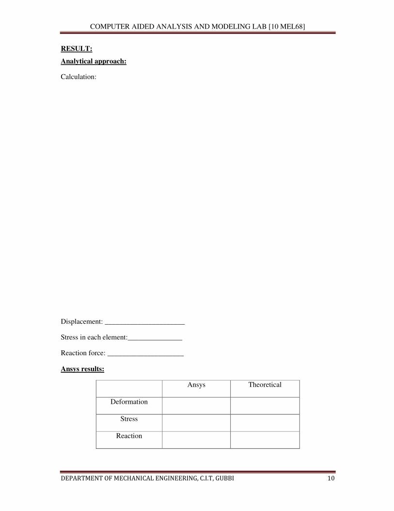
RESULT:
Analytical approach:
Calculation:
Displacement: ______________________
Stress in each element:_______________
Reaction force: _____________________
Ansys results:
Ansys Theoretical
Deformation
Stress
Reaction
COMPUTER AIDED ANALYSIS AND MODELING LAB [10 MEL68]
DEPARTMENT OF MECHANICAL ENGINEERING, C.I.T, GUBBI 11
2. TRUSSES
Problem 2.1: Consider the four bar truss shown in figure. For the given data, find Stress
in each element, Reaction forces, Nodal displacement. E = 210 GPa, A = 0.1 m2.
1. Ansys Main Menu – Preferences-select – STRUCTURAL- h method – ok
2. Element type – Add/Edit/Delete – Add – Link – 3D Finit stn 180 – ok – close.
3. Real constants – Add – ok – real constant set no – 1 – c/s area – 0.1 – ok – close.
4. Material Properties – material models – Structural – Linear – Elastic – Isotropic – EX
– 210e9– Ok – close.
5. Modeling – Create – Nodes – In Active CS – Apply (first node is created) – x,y,z
location in CS– 4 (x value w.r.t first node) – apply (second node is created) – x,y,z
location in CS – 4, 3 (x, y value w.r.t first node) – apply (third node is created) – 0, 3
(x, y value w.r.t first node) – ok (forth node is created).
6. Create–Elements–Elem Attributes – Material number – 1 – Real constant set number
– 1 – ok
7. Auto numbered – Thru Nodes – pick 1 & 2 – apply – pick 2 & 3 – apply – pick 3 & 1
– apply pick 3 & 4 – ok (elements are created through nodes).
8. Loads – Define loads – apply – Structural – Displacement – on Nodes – pick node 1
& 4 – apply – DOFs to be constrained – All DOF – ok – on Nodes – pick node 2 –
apply – DOFs to be constrained – UY – ok.
9. Loads – Define loads – apply – Structural – Force/Moment – on Nodes- pick node 2 –
apply – direction of For/Mom – FX – Force/Moment value – 2000 (+ve value) – ok –
Structural –
10. Force/Moment – on Nodes- pick node 3 – apply – direction of For/Mom – FY –
Force/Moment value – -2500 (-ve value) – ok.
11. Solve – current LS – ok (Solution is done is displayed) – close.
12. Element table – Define table – Add –‘Results data item’ – By Sequence num – LS –
LS1 – ok.
13. Plot results – contour plot –Element table – item to be plotted LS,1, avg common
nodes- yes average- ok.
14. Reaction forces: List Results – reaction solution – items to be listed – All items – ok
(reaction forces will be displayed with the node numbers).
15. Plot results- nodal solution-ok-DOF solution- Y component of displacement-ok.
16. Animation: PlotCtrls – Animate – Deformed shape – def+undeformed-ok.
COMPUTER AIDED ANALYSIS AND MODELING LAB [10 MEL68]
DEPARTMENT OF MECHANICAL ENGINEERING, C.I.T, GUBBI 12
RESULT:
Analytical approach:
Calculation:
COMPUTER AIDED ANALYSIS AND MODELING LAB [10 MEL68]
DEPARTMENT OF MECHANICAL ENGINEERING, C.I.T, GUBBI 13
Displacement: ______________________
Stress: ____________________________
Reaction force: _____________________
Ansys results:
Ansys Theoretical
Deformation
Stress
Reaction
COMPUTER AIDED ANALYSIS AND MODELING LAB [10 MEL68]
DEPARTMENT OF MECHANICAL ENGINEERING, C.I.T, GUBBI 14
Problem 2.2: Consider the two bar truss shown in figure. For the given data, find Stress
in each element, Reaction forces, Nodal displacement. E = 210 GPa, A = 0.1 m2.
1. Ansys Main Menu – Preferences-select – STRUCTURAL- h method – ok
2. Element type – Add/Edit/Delete – Add – Link – 3D Finit stn 180 – ok – close.
3. Real constants – Add – ok – real constant set no – 1 – c/s area – 0.1 – ok – close.
4. Material Properties – material models – Structural – Linear – Elastic – Isotropic – EX
– 210e9– Ok – close.
5. Modeling – Create – Nodes – In Active CS – Apply (first node is created) – x,y,z
location in CS– 0.75 (x value w.r.t first node) – apply (second node is created) – x,y,z
location in CS –(0, -0.5),(x, y value w.r.t first node) – ok (third node is created
6. Create–Elements–Elem Attributes – Material number – 1 – Real constant set number
– 1 – ok
7. Auto numbered – Thru Nodes – pick 1 & 2 – apply – pick 2 & 3–– ok (elements are
created through nodes).
8. Loads – Define loads – apply – Structural – Displacement – on Nodes – pick node 1
&3 – apply – DOFs to be constrained – All DOF – ok
9. Loads – Define loads – apply – Structural – Force/Moment – on Nodes- pick node 2 –
apply – direction of For/Mom – FY – Force/Moment value – 5000 (-ve value)
10. Solve – current LS – ok (Solution is done is displayed) – close.
11. Element table – Define table – Add –‘Results data item’ – By Sequence num – LS –
LS1 – ok.
12. Plot results – contour plot –Element table – item to be plotted LS,1, avg common
nodes- yes average- ok.
13. List Results – reaction solution – items to be listed – All items – ok (reaction forces
will be displayed with the node numbers).
14. Plot results- nodal solution-ok-DOF solution- Y component of displacement-ok.
15. Animation: PlotCtrls – Animate – Deformed shape – def+undeformed-ok.
COMPUTER AIDED ANALYSIS AND MODELING LAB [10 MEL68]
DEPARTMENT OF MECHANICAL ENGINEERING, C.I.T, GUBBI 15
RESULT:
Analytical approach:
Calculation:
COMPUTER AIDED ANALYSIS AND MODELING LAB [10 MEL68]
DEPARTMENT OF MECHANICAL ENGINEERING, C.I.T, GUBBI 16
Displacement: ______________________
Stress: ____________________________
Reaction force: _____________________
Ansys results:
Ansys Theoretical
Deformation
Stress
Reaction
COMPUTER AIDED ANALYSIS AND MODELING LAB [10 MEL68]
DEPARTMENT OF MECHANICAL ENGINEERING, C.I.T, GUBBI 17
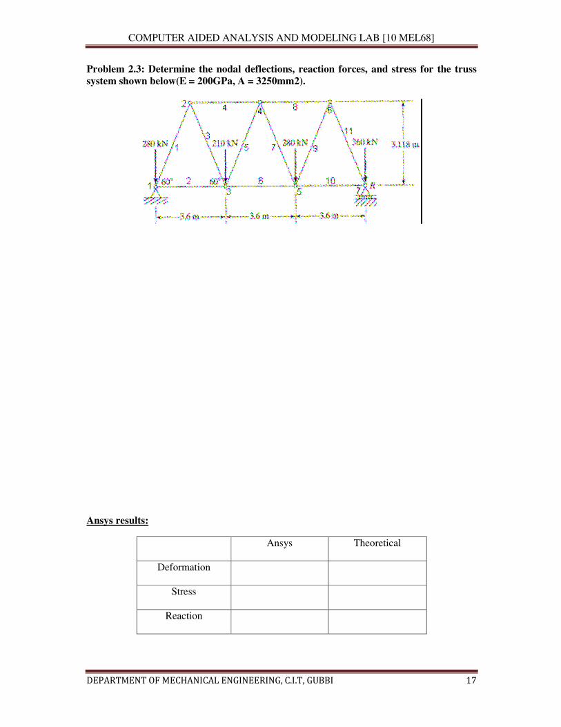
Problem 2.3: Determine the nodal deflections, reaction forces, and stress for the truss
system shown below(E = 200GPa, A = 3250mm2).
Ansys results:
Ansys Theoretical
Deformation
Stress
Reaction
COMPUTER AIDED ANALYSIS AND MODELING LAB [10 MEL68]
DEPARTMENT OF MECHANICAL ENGINEERING, C.I.T, GUBBI 18
3. BEAMS
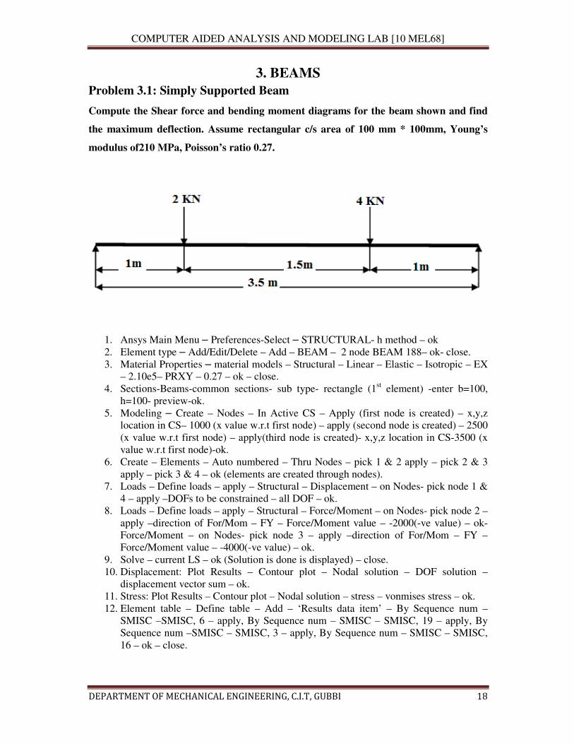
Problem 3.1: Simply Supported Beam
Compute the Shear force and bending moment diagrams for the beam shown and find
the maximum deflection. Assume rectangular c/s area of 100 mm * 100mm, Young’s
modulus of210 MPa, Poisson’s ratio 0.27.
1. Ansys Main Menu – Preferences-Select – STRUCTURAL- h method – ok
2. Element type – Add/Edit/Delete – Add – BEAM – 2 node BEAM 188– ok- close.
3. Material Properties – material models – Structural – Linear – Elastic – Isotropic – EX
– 2.10e5– PRXY – 0.27 – ok – close.
4. Sections-Beams-common sections- sub type- rectangle (1st element) -enter b=100,
h=100- preview-ok.
5. Modeling – Create – Nodes – In Active CS – Apply (first node is created) – x,y,z
location in CS– 1000 (x value w.r.t first node) – apply (second node is created) – 2500
(x value w.r.t first node) – apply(third node is created)- x,y,z location in CS-3500 (x
value w.r.t first node)-ok.
6. Create – Elements – Auto numbered – Thru Nodes – pick 1 & 2 apply – pick 2 & 3
apply – pick 3 & 4 – ok (elements are created through nodes).
7. Loads – Define loads – apply – Structural – Displacement – on Nodes- pick node 1 &
4 – apply –DOFs to be constrained – all DOF – ok.
8. Loads – Define loads – apply – Structural – Force/Moment – on Nodes- pick node 2 –
apply –direction of For/Mom – FY – Force/Moment value – -2000(-ve value) – ok-
Force/Moment – on Nodes- pick node 3 – apply –direction of For/Mom – FY –
Force/Moment value – -4000(-ve value) – ok.
9. Solve – current LS – ok (Solution is done is displayed) – close.
10. Displacement: Plot Results – Contour plot – Nodal solution – DOF solution –
displacement vector sum – ok.
11. Stress: Plot Results – Contour plot – Nodal solution – stress – vonmises stress – ok.
12. Element table – Define table – Add – ‘Results data item’ – By Sequence num –
SMISC –SMISC, 6 – apply, By Sequence num – SMISC – SMISC, 19 – apply, By
Sequence num –SMISC – SMISC, 3 – apply, By Sequence num – SMISC – SMISC,
16 – ok – close.
COMPUTER AIDED ANALYSIS AND MODELING LAB [10 MEL68]
DEPARTMENT OF MECHANICAL ENGINEERING, C.I.T, GUBBI 19
13. Plot results – contour plot – Line Element Results – Elem table item at node I –
SMIS6 – Elem table item at node J – SMIS19 – ok (Shear force diagram will be
displayed).
14. Plot results – contour plot – Line Element Results – Elem table item at node I –
SMIS3 – Elem table item at node J – SMIS16 – ok (bending moment diagram will be
displayed).
15. Reaction forces: List Results – reaction solution – items to be listed – All items – ok
(reaction forces will be displayed with the node numbers).
� NOTE: For Shear Force Diagram use the combination SMISC 6 & SMISC 19, for
Bending Moment Diagram use the combination SMISC 3 & SMISC 16.
16. Animation: PlotCtrls – Animate – Deformed results – DOF solution – USUM – ok.
RESULT:
Analytical approach:
Calculation:
COMPUTER AIDED ANALYSIS AND MODELING LAB [10 MEL68]
DEPARTMENT OF MECHANICAL ENGINEERING, C.I.T, GUBBI 20
Displacement: ______________________
Shear force: _________________________
Bending moment: ___________________
Stress:_____________________
Ansys results:
Ansys Theoretical
Deflection
Shear force
Bending moment
Stress
COMPUTER AIDED ANALYSIS AND MODELING LAB [10 MEL68]
DEPARTMENT OF MECHANICAL ENGINEERING, C.I.T, GUBBI 21
Problem 3.2: Simply Supported Beam with uniformly varying load.
Compute the Shear force and bending moment diagrams for the beam shown and find
the maximum deflection. Assume rectangular c/s area of 100mm * 100m m, Young’s
modulus of 2.1×10⁵
N/mm2, Poisson’s ratio= 0.27.
1. Ansys Main Menu – Preferences-Select – STRUCTURAL- h method- ok
2. Element type – Add/Edit/Delete – Add – BEAM – 2 nodes Beam 188 – ok – close.
3. Material Properties – material models – Structural – Linear – Elastic – Isotropic – EX
– 2.1e5– PRXY – 0.27 –ok – close.
4. Sections-Beams-common sections- sub type- rectangle (1st element) - enter b=100,
h=100- preview-ok.
5. Modeling – Create – Nodes – In Active CS – Apply (first node is created) – x,y,z
location in CS– 3000 (x value w.r.t first node) – apply (second node is created) – 4500
(x value w.r.t first node) –apply (third node is created) – 6000 (x value w.r.t first
node) – ok (forth node is created).
6. Create – Elements – Auto numbered – Thru Nodes – pick 1 & 2 – apply – pick 2 & 3
– apply –pick 3 & 4 – ok (elements are created through nodes).
7. Loads – Define loads – apply – Structural – Displacement – on Nodes- pick node 1 &
4 – apply –DOFs to be constrained – all DOF – ok.
8. Loads – Define loads – apply – Structural – Pressure – on Beams – pick element
between nodes 1 & 2–apply–pressure value at node I– 0 (value)– pressure value at
node J – 40000–ok.
9. Loads – Define loads – apply – Structural – Force/Moment – on Nodes- pick node 3 –
apply – direction of For/Mom – FY – Force/Moment value – (-80000) (-ve value) –
ok.
10. Solve – current LS – ok (Solution is done is displayed) – close.
11. Displacement: Plot Results – Contour plot – Nodal solution – DOF solution –
displacement vector sum – ok.
12. Stress: Plot Results – Contour plot – Nodal solution – stress – von mises stress – ok.
13. Element table – Define table – Add – ‘Results data item’ – By Sequence num –
SMISC –SMISC, 6 – apply, By Sequence num – SMISC – SMISC, 19 – apply, By
Sequence num –SMISC – SMISC, 3 – apply, By Sequence num – SMISC – SMISC,
16 – ok – close.
14. Plot results – contour plot – Line Element Results – Elem table item at node I –
SMIS6 – Elem table item at node J – SMIS19 – ok (Shear force diagram will be
displayed).
COMPUTER AIDED ANALYSIS AND MODELING LAB [10 MEL68]
DEPARTMENT OF MECHANICAL ENGINEERING, C.I.T, GUBBI 22
15. Plot results – contour plot – Line Element Results – Elem table item at node I –
SMIS3 – Elem table item at node J – SMIS16 – ok (bending moment diagram will be
displayed).
16. Reaction forces: List Results – reaction solution – items to be listed – All items – ok
(reaction forces will be displayed with the node numbers).
17. Animation: PlotCtrls – Animate – Deformed results – DOF solution – deformed +
undeformed – ok.
RESULT:
Analytical approach:
Calculation:
Deflection:______________________
Shear force: ________________________
Bending moment:___________________
Stress:_____________________________
Ansys results:
Ansys Theoretical
Deflection
Shear force
Bending moment
Stress
COMPUTER AIDED ANALYSIS AND MODELING LAB [10 MEL68]
DEPARTMENT OF MECHANICAL ENGINEERING, C.I.T, GUBBI 23
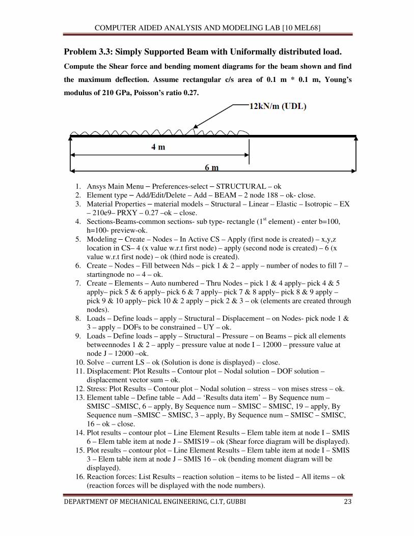
Problem 3.3: Simply Supported Beam with Uniformally distributed load.
Compute the Shear force and bending moment diagrams for the beam shown and find
the maximum deflection. Assume rectangular c/s area of 0.1 m * 0.1 m, Young’s
modulus of 210 GPa, Poisson’s ratio 0.27.
1. Ansys Main Menu – Preferences-select – STRUCTURAL – ok
2. Element type – Add/Edit/Delete – Add – BEAM – 2 node 188 – ok- close.
3. Material Properties – material models – Structural – Linear – Elastic – Isotropic – EX
– 210e9– PRXY – 0.27 –ok – close.
4. Sections-Beams-common sections- sub type- rectangle (1st element) - enter b=100,
h=100- preview-ok.
5. Modeling – Create – Nodes – In Active CS – Apply (first node is created) – x,y,z
location in CS– 4 (x value w.r.t first node) – apply (second node is created) – 6 (x
value w.r.t first node) – ok (third node is created).
6. Create – Nodes – Fill between Nds – pick 1 & 2 – apply – number of nodes to fill 7 –
startingnode no – 4 – ok.
7. Create – Elements – Auto numbered – Thru Nodes – pick 1 & 4 apply– pick 4 & 5
apply– pick 5 & 6 apply– pick 6 & 7 apply– pick 7 & 8 apply– pick 8 & 9 apply –
pick 9 & 10 apply– pick 10 & 2 apply – pick 2 & 3 – ok (elements are created through
nodes).
8. Loads – Define loads – apply – Structural – Displacement – on Nodes- pick node 1 &
3 – apply – DOFs to be constrained – UY – ok.
9. Loads – Define loads – apply – Structural – Pressure – on Beams – pick all elements
betweennodes 1 & 2 – apply – pressure value at node I – 12000 – pressure value at
node J – 12000 –ok.
10. Solve – current LS – ok (Solution is done is displayed) – close.
11. Displacement: Plot Results – Contour plot – Nodal solution – DOF solution –
displacement vector sum – ok.
12. Stress: Plot Results – Contour plot – Nodal solution – stress – von mises stress – ok.
13. Element table – Define table – Add – ‘Results data item’ – By Sequence num –
SMISC –SMISC, 6 – apply, By Sequence num – SMISC – SMISC, 19 – apply, By
Sequence num –SMISC – SMISC, 3 – apply, By Sequence num – SMISC – SMISC,
16 – ok – close.
14. Plot results – contour plot – Line Element Results – Elem table item at node I – SMIS
6 – Elem table item at node J – SMIS19 – ok (Shear force diagram will be displayed).
15. Plot results – contour plot – Line Element Results – Elem table item at node I – SMIS
3 – Elem table item at node J – SMIS 16 – ok (bending moment diagram will be
displayed).
16. Reaction forces: List Results – reaction solution – items to be listed – All items – ok
(reaction forces will be displayed with the node numbers).
COMPUTER AIDED ANALYSIS AND MODELING LAB [10 MEL68]
DEPARTMENT OF MECHANICAL ENGINEERING, C.I.T, GUBBI 24
17. PlotCtrls – Animate – Deformed results – DOF solution – USUM – ok.
RESULT:
Analytical approach:
Calculation:
Deflection:______________________
Shear force: ________________________
Bending moment: ___________________
Stress:_____________________________
Ansys results:
Ansys Theoretical
Deflection
Shear force
Bending moment
Stress
COMPUTER AIDED ANALYSIS AND MODELING LAB [10 MEL68]
DEPARTMENT OF MECHANICAL ENGINEERING, C.I.T, GUBBI 25
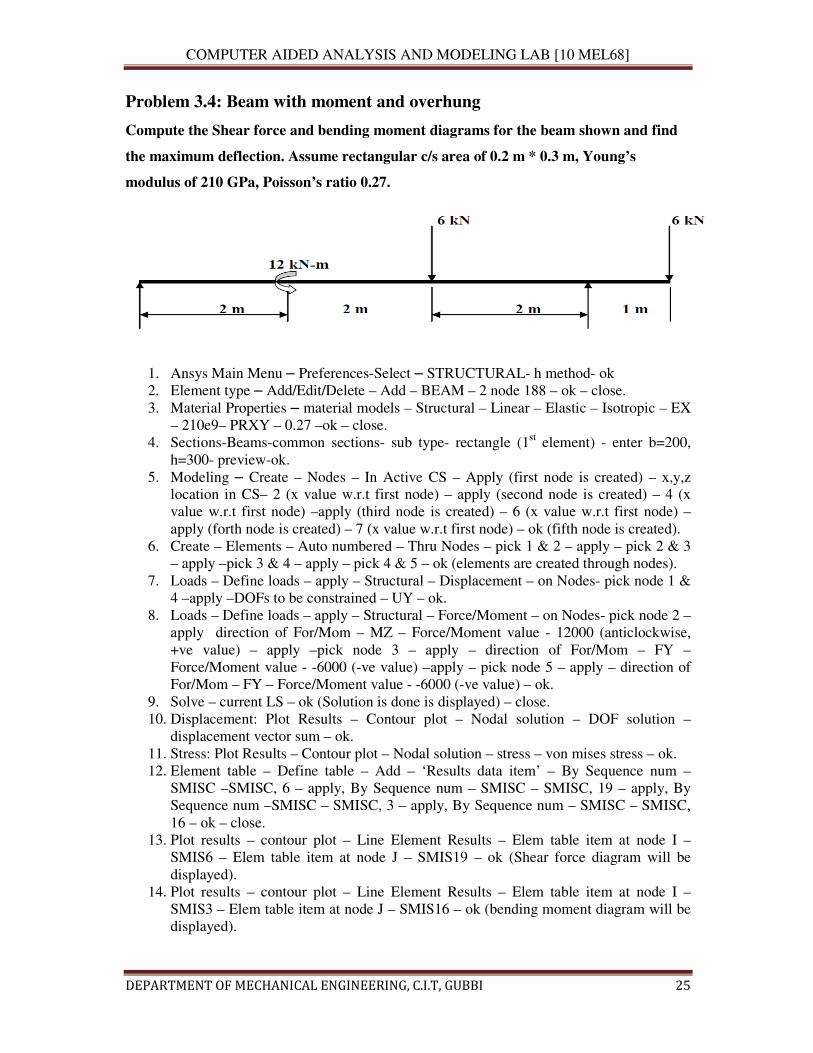
Problem 3.4: Beam with moment and overhung
Compute the Shear force and bending moment diagrams for the beam shown and find
the maximum deflection. Assume rectangular c/s area of 0.2 m * 0.3 m, Young’s
modulus of 210 GPa, Poisson’s ratio 0.27.
1. Ansys Main Menu – Preferences-Select – STRUCTURAL- h method- ok
2. Element type – Add/Edit/Delete – Add – BEAM – 2 node 188 – ok – close.
3. Material Properties – material models – Structural – Linear – Elastic – Isotropic – EX
– 210e9– PRXY – 0.27 –ok – close.
4. Sections-Beams-common sections- sub type- rectangle (1st element) - enter b=200,
h=300- preview-ok.
5. Modeling – Create – Nodes – In Active CS – Apply (first node is created) – x,y,z
location in CS– 2 (x value w.r.t first node) – apply (second node is created) – 4 (x
value w.r.t first node) –apply (third node is created) – 6 (x value w.r.t first node) –
apply (forth node is created) – 7 (x value w.r.t first node) – ok (fifth node is created).
6. Create – Elements – Auto numbered – Thru Nodes – pick 1 & 2 – apply – pick 2 & 3
– apply –pick 3 & 4 – apply – pick 4 & 5 – ok (elements are created through nodes).
7. Loads – Define loads – apply – Structural – Displacement – on Nodes- pick node 1 &
4 –apply –DOFs to be constrained – UY – ok.
8. Loads – Define loads – apply – Structural – Force/Moment – on Nodes- pick node 2 –
apply direction of For/Mom – MZ – Force/Moment value - 12000 (anticlockwise,
+ve value) – apply –pick node 3 – apply – direction of For/Mom – FY –
Force/Moment value - -6000 (-ve value) –apply – pick node 5 – apply – direction of
For/Mom – FY – Force/Moment value - -6000 (-ve value) – ok.
9. Solve – current LS – ok (Solution is done is displayed) – close.
10. Displacement: Plot Results – Contour plot – Nodal solution – DOF solution –
displacement vector sum – ok.
11. Stress: Plot Results – Contour plot – Nodal solution – stress – von mises stress – ok.
12. Element table – Define table – Add – ‘Results data item’ – By Sequence num –
SMISC –SMISC, 6 – apply, By Sequence num – SMISC – SMISC, 19 – apply, By
Sequence num –SMISC – SMISC, 3 – apply, By Sequence num – SMISC – SMISC,
16 – ok – close.
13. Plot results – contour plot – Line Element Results – Elem table item at node I –
SMIS6 – Elem table item at node J – SMIS19 – ok (Shear force diagram will be
displayed).
14. Plot results – contour plot – Line Element Results – Elem table item at node I –
SMIS3 – Elem table item at node J – SMIS16 – ok (bending moment diagram will be
displayed).
COMPUTER AIDED ANALYSIS AND MODELING LAB [10 MEL68]
DEPARTMENT OF MECHANICAL ENGINEERING, C.I.T, GUBBI 26
15. Reaction forces: List Results – reaction solution – items to be listed – All items – ok
(reaction forces will be displayed with the node numbers).
16. Animation: PlotCtrls – Animate – Deformed results – DOF solution – deformed +
undeformed – ok.
RESULT:
Analytical approach:
Calculation:
Deflection: ______________________
Shear force: ________________________
Bending moment:____________________
Stress: ____________________
Ansys results:
Ansys Theoretical
Deflection
SFD
BMD
Stress
COMPUTER AIDED ANALYSIS AND MODELING LAB [10 MEL68]
DEPARTMENT OF MECHANICAL ENGINEERING, C.I.T, GUBBI 27
Problem 3.5: Cantilever Beam
Compute the Shear force and bending moment diagrams for the beam shown and find
the maximum deflection. Assume rectangular c/s area of 0.2 m * 0.3 m, Young’s
modulus of 210 GPa, Poisson’s ratio 0.27.
1. Ansys Main Menu – Preferences-Select – STRUCTURAL- h method – ok
2. Element type – Add/Edit/Delete – Add – BEAM – 2 node Beam 188 – ok- close.
3. Material Properties – material models – Structural – Linear – Elastic – Isotropic – EX
– 210e9– PRXY – 0.27 –ok – close.
4. Sections-Beams-common sections- sub type- rectangle (1st element) - enter b=200,
h=300- preview-ok.
5. Modeling – Create – Nodes – In Active CS – Apply (first node is created) – x,y,z
location in CS– 2 (x value w.r.t first node) – ok (second node is created).
6. Create – Elements – Auto numbered – Thru Nodes – pick 1 & 2 – ok (elements are
created through nodes).
7. Loads – Define loads – apply – Structural – Displacement – on Nodes- pick node 1 –
apply –
8. DOFs to be constrained – ALL DOF – ok.
9. Loads – Define loads – apply – Structural – Force/Moment – on Nodes- pick node 2 –
apply – direction of For/Mom – FY – Force/Moment value –( -40000) (-ve value) –
ok.
10. Solve – current LS – ok (Solution is done is displayed) – close.
11. Displacement: Plot Results – Contour plot – Nodal solution – DOF solution –
displacement vector sum – ok.
12. Stress: Plot Results – Contour plot – Nodal solution – stress – von mises stress – ok.
13. Element table – Define table – Add – ‘Results data item’ – By Sequence num –
SMISC –SMISC, 6 – apply, By Sequence num – SMISC – SMISC, 19 – apply, By
Sequence num –SMISC – SMISC, 3 – apply, By Sequence num – SMISC – SMISC,
16 – ok – close.
14. Plot results – contour plot – Line Element Results – Elem table item at node I –
SMIS6 – Elem table item at node J – SMIS19 – ok (Shear force diagram will be
displayed).
15. Plot results – contour plot – Line Element Results – Elem table item at node I –
SMIS3 – Elem table item at node J – SMIS16 – ok (bending moment diagram will be
displayed).
16. Reaction forces: List Results – reaction solution – items to be listed – All items – ok
(reaction forces will be displayed with the node numbers).
COMPUTER AIDED ANALYSIS AND MODELING LAB [10 MEL68]
DEPARTMENT OF MECHANICAL ENGINEERING, C.I.T, GUBBI 28
RESULT:
Analytical approach:
Calculation:
Deflection: ______________________
Shear force: ________________________
Bending moment: ____________________
Stress: _____________________
Ansys results:
Ansys Theoretical
Deflection
SFD
BMD
Stress
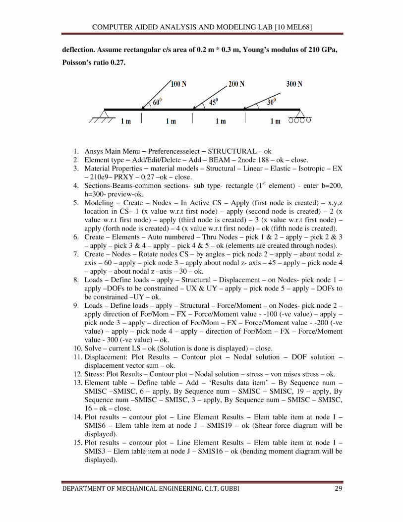
Problem 3.6: Beam with angular loads
Compute the Shear force and bending moment diagrams for the beam shown in fig such
thatone end hinged and at the other end is having roller support and find the maximum
COMPUTER AIDED ANALYSIS AND MODELING LAB [10 MEL68]
DEPARTMENT OF MECHANICAL ENGINEERING, C.I.T, GUBBI 29
deflection. Assume rectangular c/s area of 0.2 m * 0.3 m, Young’s modulus of 210 GPa,
Poisson’s ratio 0.27.
1. Ansys Main Menu – Preferencesselect – STRUCTURAL – ok
2. Element type – Add/Edit/Delete – Add – BEAM – 2node 188 – ok – close.
3. Material Properties – material models – Structural – Linear – Elastic – Isotropic – EX
– 210e9– PRXY – 0.27 –ok – close.
4. Sections-Beams-common sections- sub type- rectangle (1st element) - enter b=200,
h=300- preview-ok.
5. Modeling – Create – Nodes – In Active CS – Apply (first node is created) – x,y,z
location in CS– 1 (x value w.r.t first node) – apply (second node is created) – 2 (x
value w.r.t first node) – apply (third node is created) – 3 (x value w.r.t first node) –
apply (forth node is created) – 4 (x value w.r.t first node) – ok (fifth node is created).
6. Create – Elements – Auto numbered – Thru Nodes – pick 1 & 2 – apply – pick 2 & 3
– apply – pick 3 & 4 – apply – pick 4 & 5 – ok (elements are created through nodes).
7. Create – Nodes – Rotate nodes CS – by angles – pick node 2 – apply – about nodal z-
axis – 60 – apply – pick node 3 – apply about nodal z- axis – 45 – apply – pick node 4
– apply – about nodal z –axis – 30 – ok.
8. Loads – Define loads – apply – Structural – Displacement – on Nodes- pick node 1 –
apply –DOFs to be constrained – UX & UY – apply – pick node 5 – apply – DOFs to
be constrained –UY – ok.
9. Loads – Define loads – apply – Structural – Force/Moment – on Nodes- pick node 2 –
apply direction of For/Mom – FX – Force/Moment value - -100 (-ve value) – apply –
pick node 3 – apply – direction of For/Mom – FX – Force/Moment value - -200 (-ve
value) – apply – pick node 4 – apply – direction of For/Mom – FX – Force/Moment
value - 300 (-ve value) – ok.
10. Solve – current LS – ok (Solution is done is displayed) – close.
11. Displacement: Plot Results – Contour plot – Nodal solution – DOF solution –
displacement vector sum – ok.
12. Stress: Plot Results – Contour plot – Nodal solution – stress – von mises stress – ok.
13. Element table – Define table – Add – ‘Results data item’ – By Sequence num –
SMISC –SMISC, 6 – apply, By Sequence num – SMISC – SMISC, 19 – apply, By
Sequence num –SMISC – SMISC, 3 – apply, By Sequence num – SMISC – SMISC,
16 – ok – close.
14. Plot results – contour plot – Line Element Results – Elem table item at node I –
SMIS6 – Elem table item at node J – SMIS19 – ok (Shear force diagram will be
displayed).
15. Plot results – contour plot – Line Element Results – Elem table item at node I –
SMIS3 – Elem table item at node J – SMIS16 – ok (bending moment diagram will be
displayed).
COMPUTER AIDED ANALYSIS AND MODELING LAB [10 MEL68]
DEPARTMENT OF MECHANICAL ENGINEERING, C.I.T, GUBBI 30
RESULT:
Analytical approach:
Calculation:
COMPUTER AIDED ANALYSIS AND MODELING LAB [10 MEL68]
DEPARTMENT OF MECHANICAL ENGINEERING, C.I.T, GUBBI 31
Deflection:______________________
Shear force: ________________________
Bending moment: ___________________
Stress:_____________________________
Ansys results:
Ansys Theoretical
Deflection
Shear force
Bending moment
Stress
PART B
Stress analysis of a rectangular plate with circular hole
Problem 4.1: In the plate with a hole under plane stress, find deformed shape of the hole
and determine the maximum stress distribution along A-B (you may use t = 1 mm). E =
210GPa, t = 1 mm, Poisson’s ratio = 0.3, Dia of the circle = 10 mm, Analysis assumption
– plane stress with thickness is used.
COMPUTER AIDED ANALYSIS AND MODELING LAB [10 MEL68]
DEPARTMENT OF MECHANICAL ENGINEERING, C.I.T, GUBBI 32
1. Ansys Main Menu – Preferences-Select – STRUCTURAL-h method – ok
2. Element type – Add/Edit/Delete – Add – Solid – Quad 4 node – 42 – ok – option –
element behavior K3 – Plane stress with thickness – ok – close.
3. Real constants – Add – ok – real constant set no – 1 – Thickness – 1 – ok.
4. Material Properties – material models – Structural – Linear – Elastic – Isotropic – EX
– 2.1e5 –PRXY – 0.3 – ok – close.
5. Modeling –Create – Area – Rectangle – by dimensions – X1, X2, Y1, Y2 – 0, 60, 0,
40 – ok.
6. Create – Area – Circle – solid circle – X, Y, radius – 30, 20, 5 – ok.
7. Operate – Booleans – Subtract – Areas – pick area which is not to be deleted
(rectangle) – apply – pick area which is to be deleted (circle) – ok.
8. Meshing – Mesh Tool – Mesh Areas – Quad – Free – Mesh – pick all – ok. Mesh
Tool – Refine – pick all – Level of refinement – 3 – ok.
9. Loads – Define loads – apply – Structural – Displacement – on Nodes – select box –
drag the left side of the area – apply – DOFs to be constrained – ALL DOF – ok.
10. Loads – Define loads – apply – Structural – Force/Moment – on Nodes – select box –
drag the right side of the area – apply – direction of For/Mom – FX – Force/Moment
value – 2000 (+ve value) – ok.
11. Solve – current LS – ok (Solution is done is displayed) – close.
12. Deformed shape-Plot Results – Deformed Shape – def+undeformed – ok.
13. Plot results – contour plot – Element solu – Stress – Von Mises Stress – ok (the stress
distribution diagram will be displayed).
RESULT:
Analytical approach:
Calculation:
COMPUTER AIDED ANALYSIS AND MODELING LAB [10 MEL68]
DEPARTMENT OF MECHANICAL ENGINEERING, C.I.T, GUBBI 33
Ansys results:
Ansys Theoretical
Deformation
Stress
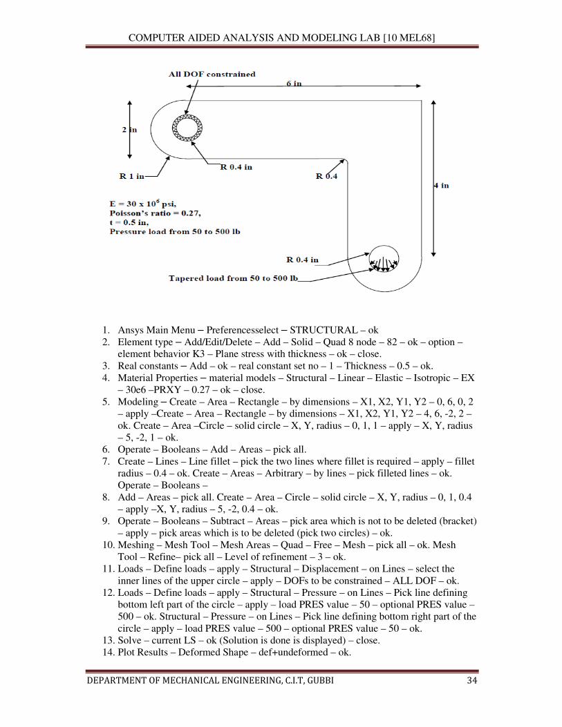
Problem 4.2: The corner angle bracket is shown below. The upper left hand pin-hole is
constrained around its entire circumference and a tapered pressure load is applied to
the bottom of lower right hand pin-hole. Compute Maximum displacement, Von-Mises
stress.
COMPUTER AIDED ANALYSIS AND MODELING LAB [10 MEL68]
DEPARTMENT OF MECHANICAL ENGINEERING, C.I.T, GUBBI 34
1. Ansys Main Menu – Preferencesselect – STRUCTURAL – ok
2. Element type – Add/Edit/Delete – Add – Solid – Quad 8 node – 82 – ok – option –
element behavior K3 – Plane stress with thickness – ok – close.
3. Real constants – Add – ok – real constant set no – 1 – Thickness – 0.5 – ok.
4. Material Properties – material models – Structural – Linear – Elastic – Isotropic – EX
– 30e6 –PRXY – 0.27 – ok – close.
5. Modeling – Create – Area – Rectangle – by dimensions – X1, X2, Y1, Y2 – 0, 6, 0, 2
– apply –Create – Area – Rectangle – by dimensions – X1, X2, Y1, Y2 – 4, 6, -2, 2 –
ok. Create – Area –Circle – solid circle – X, Y, radius – 0, 1, 1 – apply – X, Y, radius
– 5, -2, 1 – ok.
6. Operate – Booleans – Add – Areas – pick all.
7. Create – Lines – Line fillet – pick the two lines where fillet is required – apply – fillet
radius – 0.4 – ok. Create – Areas – Arbitrary – by lines – pick filleted lines – ok.
Operate – Booleans –
8. Add – Areas – pick all. Create – Area – Circle – solid circle – X, Y, radius – 0, 1, 0.4
– apply –X, Y, radius – 5, -2, 0.4 – ok.
9. Operate – Booleans – Subtract – Areas – pick area which is not to be deleted (bracket)
– apply – pick areas which is to be deleted (pick two circles) – ok.
10. Meshing – Mesh Tool – Mesh Areas – Quad – Free – Mesh – pick all – ok. Mesh
Tool – Refine– pick all – Level of refinement – 3 – ok.
11. Loads – Define loads – apply – Structural – Displacement – on Lines – select the
inner lines of the upper circle – apply – DOFs to be constrained – ALL DOF – ok.
12. Loads – Define loads – apply – Structural – Pressure – on Lines – Pick line defining
bottom left part of the circle – apply – load PRES value – 50 – optional PRES value –
500 – ok. Structural – Pressure – on Lines – Pick line defining bottom right part of the
circle – apply – load PRES value – 500 – optional PRES value – 50 – ok.
13. Solve – current LS – ok (Solution is done is displayed) – close.
14. Plot Results – Deformed Shape – def+undeformed – ok.
COMPUTER AIDED ANALYSIS AND MODELING LAB [10 MEL68]
DEPARTMENT OF MECHANICAL ENGINEERING, C.I.T, GUBBI 35
15. Plot results – contour plot – Element solu – Stress – Von Mises Stress – ok (the stress
distribution diagram will be displayed).
16. PlotCtrls – Animate – Deformed shape – def+undeformed-ok.
RESULT:
COMPUTER AIDED ANALYSIS AND MODELING LAB [10 MEL68]
DEPARTMENT OF MECHANICAL ENGINEERING, C.I.T, GUBBI 36
THERMAL ANALYSIS
Problem 5.1: Solve the 2-D heat conduction problem for the temperature distribution
within the rectangular plate. Thermal conductivity of the plate, KXX=401 W/(m-K).
1. Ansys Main Menu – Preferences-select – THERMAL- h method– ok
2. Element type – Add/Edit/Delete – Add – Solid – Quad 4 node – 55 – ok – option –
elementbehavior K3 – Plane stress with thickness – ok – close.
3. Material Properties – material models – Thermal – Conductivity – Isotropic – KXX –
401.
4. Modeling – Create – Area – Rectangle – by dimensions – X1, X2, Y1, Y2 – 0, 10, 0,
20 – ok.
5. Meshing – Mesh Tool – Mesh Areas – Quad – Free – Mesh – pick all – ok. Mesh
Tool – Refine – pick all – Level of refinement – 3 – ok.
6. Loads – Define loads – apply – Thermal – Temperature – on Lines – select 1000 C
lines – apply – DOFs to be constrained – TEMP – Temp value – 1000 C – ok.
7. Loads – Define loads – apply – Thermal – Temperature – on Lines – select 1000 C
lines –
8. Solve – current LS – ok (Solution is done is displayed) – close.
9. Read results-last set-ok
10. List results-nodal solution-select temperature-ok
11. Observe the nodal solution per node.
12. From the menu bar-plot ctrls-style-size and shape-display of the element-click on real
constant multiplier=0.2, don’t change other values-ok.
13. Plot results-contour plot-nodal solution-temperature-deformed shape only-ok
14. Element table-define table-add-enter user label item=HTRANS, select by sequence no
SMISC, 1-ok-close.
15. Element table-list table-select HTRANS-ok
COMPUTER AIDED ANALYSIS AND MODELING LAB [10 MEL68]
DEPARTMENT OF MECHANICAL ENGINEERING, C.I.T, GUBBI 37
RESULT:
COMPUTER AIDED ANALYSIS AND MODELING LAB [10 MEL68]
DEPARTMENT OF MECHANICAL ENGINEERING, C.I.T, GUBBI 38
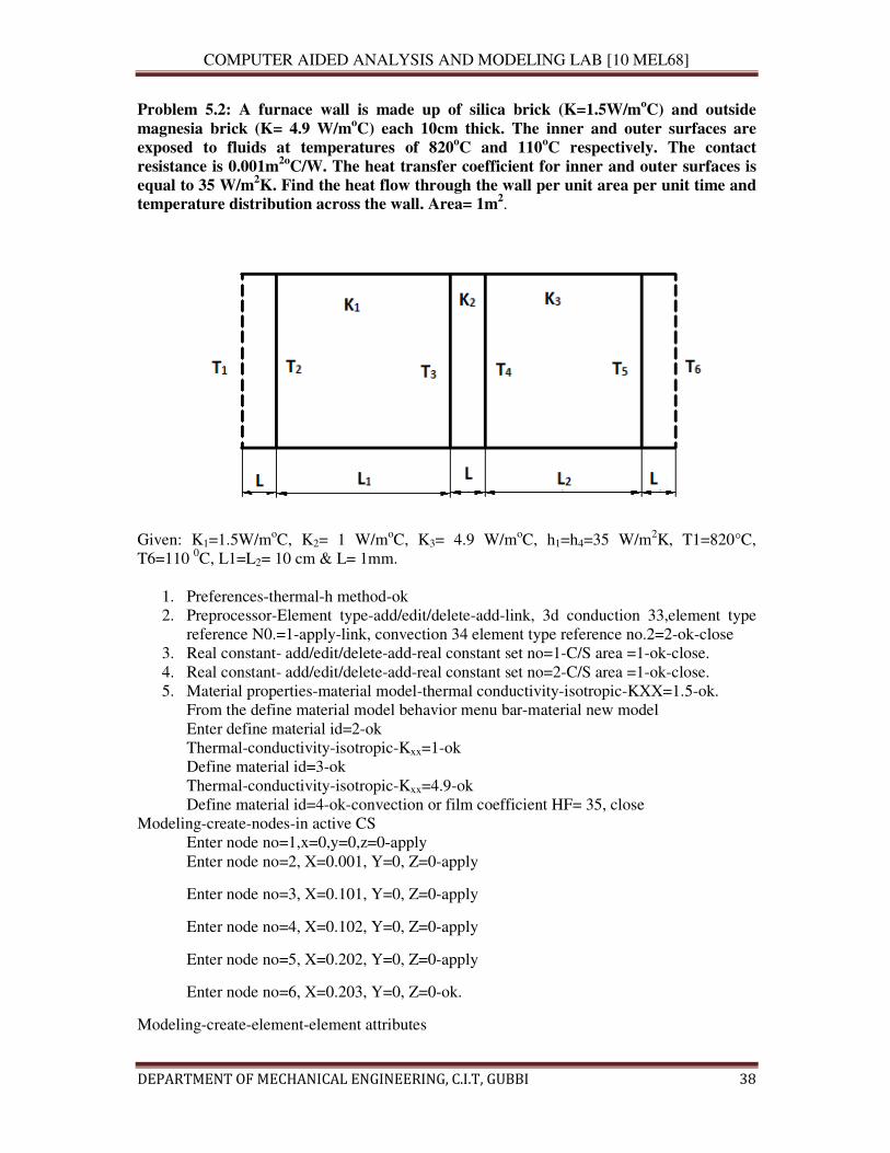
Problem 5.2: A furnace wall is made up of silica brick (K=1.5W/moC) and outside
magnesia brick (K= 4.9 W/moC) each 10cm thick. The inner and outer surfaces are
exposed to fluids at temperatures of 820oC and 110
oC respectively. The contact
resistance is 0.001m2o
C/W. The heat transfer coefficient for inner and outer surfaces is
equal to 35 W/m2K. Find the heat flow through the wall per unit area per unit time and
temperature distribution across the wall. Area= 1m2.
Given: K1=1.5W/moC, K2= 1 W/m
oC, K3= 4.9 W/m
oC, h1=h4=35 W/m
2K, T1=820°C,
T6=110 0C, L1=L2= 10 cm & L= 1mm.
1. Preferences-thermal-h method-ok
2. Preprocessor-Element type-add/edit/delete-add-link, 3d conduction 33,element type
reference N0.=1-apply-link, convection 34 element type reference no.2=2-ok-close
3. Real constant- add/edit/delete-add-real constant set no=1-C/S area =1-ok-close.
4. Real constant- add/edit/delete-add-real constant set no=2-C/S area =1-ok-close.
5. Material properties-material model-thermal conductivity-isotropic-KXX=1.5-ok.
From the define material model behavior menu bar-material new model
Enter define material id=2-ok
Thermal-conductivity-isotropic-Kxx=1-ok
Define material id=3-ok
Thermal-conductivity-isotropic-Kxx=4.9-ok
Define material id=4-ok-convection or film coefficient HF= 35, close
Modeling-create-nodes-in active CS
Enter node no=1,x=0,y=0,z=0-apply
Enter node no=2, X=0.001, Y=0, Z=0-apply
Enter node no=3, X=0.101, Y=0, Z=0-apply
Enter node no=4, X=0.102, Y=0, Z=0-apply
Enter node no=5, X=0.202, Y=0, Z=0-apply
Enter node no=6, X=0.203, Y=0, Z=0-ok.
Modeling-create-element-element attributes
COMPUTER AIDED ANALYSIS AND MODELING LAB [10 MEL68]
DEPARTMENT OF MECHANICAL ENGINEERING, C.I.T, GUBBI 39
Enter element type no=2 LINK 34 (convection)
Material no=4 (convection or film coefficient)
Real constant set no=2 (convection)-ok
Modeling-create-element-auto numbered-through node-pick the nodes 1 & 2-ok
Modeling-create-element-element attributes
Enter element type no=1 LINK 33 (Conduction)
Material no=1 (conduction)
Real constant set no=1 (conduction)-ok
Modeling-create-element-auto numbered-through node-pick the nodes 2 & 3-ok
Modeling-create-element-element attributes
Enter element type no=1 LINK 33 (Conduction)
Material no=2 (conduction)
Real constant set no=1 (conduction)-ok
Modeling-create-element-auto numbered-through node-pick the nodes 3 & 4-ok
Modeling-create-element-element attributes
Enter element type no=1 LINK 33 (Conduction)
Material no=3 (conduction)
Real constant set no=1 (conduction)-ok
Modeling-create-element-auto numbered-through node-pick the nodes 4 & 5-ok.
Modeling-create-element-element attributes
Enter element type no=2 LINK 34 (Convection)
Material no=4 (convection or film coefficient)
Real constant set no=2 (convection)-ok
Modeling-create-element-auto numbered-through node-pick the nodes 5 & 6-ok.
Observe the straight line.
From the menu bar select plot controls-Numbering-Plot numbering control and select
element/attributes numbering=element no and don’t change other attributes-ok
6. Solution- Analysis type-new analysis-steady state-ok.
• Solution-define loads-apply-thermal-temperature-on nodes-pick the first nodes-ok-
temperature-load-temperature value=8200 C-apply.
COMPUTER AIDED ANALYSIS AND MODELING LAB [10 MEL68]
DEPARTMENT OF MECHANICAL ENGINEERING, C.I.T, GUBBI 40
• Define load-apply-thermal-temperature-on nodes-pick the last node-ok, select
temperature-load temperature value=1100 C-ok.
• Solution- solve-current LS-ok.
Solution is done-close.
7. Read results-last set-ok
8. List results-nodal solution-select temperature-ok
9. Observe the nodal solution per node.
10. From the menu bar-plot ctrls-style-size and shape-display of the element-click on real
constant multiplier=0.2, don’t change other values-ok.
11. Plot results-contour plot-nodal solution-temperature-deformed shape only-ok
12. Element table-define table-add-enter user label item=HTRANS, select by sequence no
SMISC, 1-ok-close.
13. Element table-list table-select HTRANS-ok
RESULT:
Analytical approach:
Calculation:
Ansys results:
COMPUTER AIDED ANALYSIS AND MODELING LAB [10 MEL68]
DEPARTMENT OF MECHANICAL ENGINEERING, C.I.T, GUBBI 41
Ansys Theoretical
Nodal temperature
T1
T2
T3
T4
T5
T6
Heat flux
Problem 5.3: The exterior wall of a building is constructed of four materials, 12mm
thick gypsum board, 75mm thick fibre glass insulation, 20mm thick plywood and 20mm
thick hardboard. The inside and outside air temperatures are 20oC and -10
oC
respectively. The convective heat transfer coefficients on the inner and outer surfaces of
the wall are 6W/m2 o
C and 10 W/m2 o
C respectively. Determine the heat flux and the
temperature distribution. Take K for gypsum=0.176W/moC, K for fibre
glass=0.036W/moC, K for plywood=0.115 W/m
oC and K for hardboard=0.215 W/m
oC.
Area= 1m2.
1. Preferences-thermal-h method-ok
2. Element type-add/edit/delete-add-link, 3d conduction 33,element type reference
N0.=1-apply-link, convection 34 element type reference no.2=2-ok-close
3. Real constant- add/edit/delete-add-real constant set no=1-C/S area =1-ok-close.
4. Real constant- add/edit/delete-add-real constant set no=2-C/S area =1-ok-close.
COMPUTER AIDED ANALYSIS AND MODELING LAB [10 MEL68]
DEPARTMENT OF MECHANICAL ENGINEERING, C.I.T, GUBBI 42
5. Material properties-material model-convection film coefficient-enter HF=6-ok
From the define material model behaviour menu bar-material new model
Enter define material id=2-ok
Thermal-conductivity-isotropic-Kxx=0.176-ok
Define material id=3-ok
Thermal-conductivity-isotropic-Kxx=0.036-ok
Define material id=4-ok
Thermal-conductivity-isotropic-Kxx=0.115-ok
Define material id=5-ok
Thermal-conductivity-isotropic-Kxx=0.215-ok
Define material id=6-convection or film coefficient HF= 10, close
Modeling-create-nodes-in active CS
Enter node no=1,x=0,y=0,z=0-apply
Enter node no=2, X=0.001, Y=0, Z=0-apply
Enter node no=3, X=0.013, Y=0, Z=0-apply
Enter node no=4, X=0.088, Y=0, Z=0-apply
Enter node no=5, X=0.108, Y=0, Z=0-apply
Enter node no=6, X=0.128, Y=0, Z=0-apply
Enter node no=7, X=0.129, Y=0, Z=0-ok
Modeling-create-element-element attributes
Enter element type no=2 LINK 34 (convection)
Material no=1 (convection or film coefficient)
Real constant set no=2 (convection)-ok
Modeling-create-element-auto numbered-through node-pick the nodes 1 & 2-ok
Modeling-create-element-element attributes
Enter element type no=1 LINK 33 (Conduction)
Material no=2 (conduction)
Real constant set no=1 (conduction)-ok
Modeling-create-element-auto numbered-through node-pick the nodes 2 & 3-ok
Modeling-create-element-element attributes
Enter element type no=1 LINK 33(Conduction)
Material no=3 (conduction)
Real constant set no=1 (conduction)-ok
Modeling-create-element-auto numbered-through node-pick the nodes 3 & 4-ok
COMPUTER AIDED ANALYSIS AND MODELING LAB [10 MEL68]
DEPARTMENT OF MECHANICAL ENGINEERING, C.I.T, GUBBI 43
Modeling-create-element-element attributes
Enter element type no=1 LINK 33 (Conduction)
Material no=4 (conduction)
Real constant set no=1 (conduction)-ok
Modeling-create-element-auto numbered-through node-pick the nodes 4 & 5-ok.
Modeling-create-element-element attributes
Enter element type no=1 LINK 33 (Conduction)
Material no=5 (convection or film coefficient)
Real constant set no=1 (conduction)-ok
Modeling-create-element-auto numbered-through node-pick the nodes 5 & 6-ok.
Modeling-create-element-element attributes
Enter element type no=2 LINK 34 (convection)
Material no=6 (convection or film coefficient)
Real constant set no=2 (convection)-ok
Modeling-create-element-auto numbered-through node-pick the nodes 6 & 7-ok
Observe the straight line.
From the menu bar select plot controls-Numbering-Plot numbering control and select
element/attributes numbering=element no and don’t change other attributes-ok
6. Solution- Analysis type-new analysis-steady state-ok.
• Solution-define loads-apply-thermal-temperature-on nodes-pick the first nodes-ok-
temperature-load-temperature value=200 C-apply.
• Define load-apply-thermal-temperature-on nodes-pick the last node-ok, select
temperature-load temperature value=-100 C-ok.
• Solution- solve-current LS-ok.
Solution is done-close.
7. Read results-last set-ok
8. List results-nodal solution-select temperature-ok
9. Observe the nodal solution per node.
10. From the menu bar-plot ctrls-style-size and shape-display of the element-click on real
constant multiplier=0.2, don’t change other values-ok.
11. Plot results-contour plot-nodal solution-temperature-deformed shape only-ok
12. Element table-define table-add-enter user label item=HTRANS, select by sequence no
SMISC, 1-ok-close.
13. Element table-list table-select HTRANS-ok
COMPUTER AIDED ANALYSIS AND MODELING LAB [10 MEL68]
DEPARTMENT OF MECHANICAL ENGINEERING, C.I.T, GUBBI 44
RESULT:
Analytical approach:
Calculation:
Ansys results:
Ansys Theoretical
Nodal temperature
T1
T2
T3
T4
T5
T6
T7
Heat flux
COMPUTER AIDED ANALYSIS AND MODELING LAB [10 MEL68]
DEPARTMENT OF MECHANICAL ENGINEERING, C.I.T, GUBBI 45
Problem 5.4: A plane wall ‘X’ (K=75W/mK) is 60 mm thick and has volumetric heat
generation of 1.5×10⁶W/m
3. It is insulated on one side while the other side is in contact
with the surface of another wall ‘Y’ (K=150W/mK) which is 30mm thick and has no
heat generation. The free surface of wall ‘Y’ is exposed to a cooling fluid at 200C with a
convection coefficient of 950 W/m2K. Find steady state temperatures at salient points
across the composite wall. Area= 1m2.
1. Preferences-Thermal-h method-ok
2. Element type-add/edit/delete- add-solid, quad 4node 55-enter reference number=1-
select options-element behaviour,K3= plane thickness-ok
3. Real constants- add/edit/delete-add- enter real constant set no. 1, thickness=2-ok-close
4. Material properties-Material models-material number 1-thermal-conductivity-
isotropic-KXX=75-ok.
5. From the menu bar select material-new model-enter material no. ID 2=2-select
6. Material model no.2- thermal-conductivity-isotropic-KXX=150-ok.
7. Modeling-create-areas-rectangles-by dimensions-X1=0, X2=0.06, Y1=0,Y2=0.03-
apply- X1=0.06, X2=0.09, Y1=0,Y2=0.03-OK
Modeling-operate-Boolean-glue-areas-pick the material-ok
8. Meshing-size controls-manual size-picked lines-pick the first vertical line, middle line
and the last vertical line-ok-number of element divisions-2-apply
Meshing-size controls-manual size-picked lines-pick the first rectangle top and
bottom lines-number of element divisions=60-apply
Meshing-size controls-manual size-picked lines-pick the top and bottom lines of
second rectangle-number of element divisions=30-ok.
Meshing-mesh areas- free-pick all-ok.
9. Solution-Analysis type-new analysis-steady state-ok
� define loads-apply-thermal-heat generated on areas-pick the first rectangle-ok
� define loads-apply-thermal-heat generated on areas-apply Hgen on areas as constant
value- load Hgen value=1.5e6
� define loads-apply-thermal-convection-on lines-pick the back corner line-ok-enter
film coefficient=950-bulk temperature=200C (Don’t change other attributes)-ok
COMPUTER AIDED ANALYSIS AND MODELING LAB [10 MEL68]
DEPARTMENT OF MECHANICAL ENGINEERING, C.I.T, GUBBI 46
� define loads-apply-thermal-heat flux-on lines-pick the front corner line-ok-enter heat
flux=0-ok
10. Solution-solve-current LS-ok-close
11. Read results-last set-ok
12. List results-nodal solution-select temperature-ok
13. Observe the nodal solution per node.
14. From the menu bar-plot ctrls-style-size and shape-display of the element-click on real
constant multiplier=0.2, don’t change other values-ok.
15. Plot results-contour plot-nodal solution-temperature-deformed shape only-ok
RESULT:
Analytical approach:
Calculation:
Ansys results:
Ansys Theoretical
Nodal temperature
T1
T2
T3
COMPUTER AIDED ANALYSIS AND MODELING LAB [10 MEL68]
DEPARTMENT OF MECHANICAL ENGINEERING, C.I.T, GUBBI 47
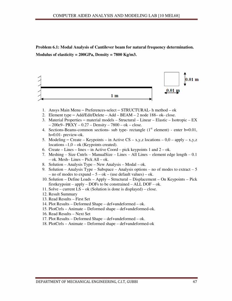
Problem 6.1: Modal Analysis of Cantilever beam for natural frequency determination.
Modulus of elasticity = 200GPa, Density = 7800 Kg/m3.
1. Ansys Main Menu – Preferences-select – STRUCTURAL- h method – ok
2. Element type – Add/Edit/Delete – Add – BEAM – 2 node 188– ok- close.
3. Material Properties – material models – Structural – Linear – Elastic – Isotropic – EX
– 200e9– PRXY – 0.27 – Density – 7800 – ok – close.
4. Sections-Beams-common sections- sub type- rectangle (1st element) - enter b=0.01,
h=0.01- preview-ok.
5. Modeling – Create – Keypoints – in Active CS – x,y,z locations – 0,0 – apply – x,y,z
locations –1,0 – ok (Keypoints created).
6. Create – Lines – lines – in Active Coord – pick keypoints 1 and 2 – ok.
7. Meshing – Size Cntrls – ManualSize – Lines – All Lines – element edge length – 0.1
– ok. Mesh– Lines – Pick All – ok.
8. Solution – Analysis Type – New Analysis – Modal – ok.
9. Solution – Analysis Type – Subspace – Analysis options – no of modes to extract – 5
– no of modes to expand – 5 – ok – (use default values) – ok.
10. Solution – Define Loads – Apply – Structural – Displacement – On Keypoints – Pick
firstkeypoint – apply – DOFs to be constrained – ALL DOF – ok.
11. Solve – current LS – ok (Solution is done is displayed) – close.
12. Result Summary
13. Read Results – First Set
14. Plot Results – Deformed Shape – def+undeformed – ok.
15. PlotCtrls – Animate – Deformed shape – def+undeformed-ok.
16. Read Results – Next Set
17. Plot Results – Deformed Shape – def+undeformed – ok.
18. PlotCtrls – Animate – Deformed shape – def+undeformed-ok
COMPUTER AIDED ANALYSIS AND MODELING LAB [10 MEL68]
DEPARTMENT OF MECHANICAL ENGINEERING, C.I.T, GUBBI 48
RESULT:
Analytical solution:
Ansys results:
COMPUTER AIDED ANALYSIS AND MODELING LAB [10 MEL68]
DEPARTMENT OF MECHANICAL ENGINEERING, C.I.T, GUBBI 49
Problem 6.2: Fixed- fixed beam subjected to forcing function
Conduct a harmonic forced response test by applying a cyclic load (harmonic) at the
end of the beam. The frequency of the load will be varied from 1 - 100 Hz. Modulus of
elasticity = 200GPa, Poisson’s ratio = 0.3, Density = 7800 Kg/m3.
1. Ansys Main Menu – Preferences-select – STRUCTURAL- h method – ok
2. Element type – Add/Edit/Delete – Add – BEAM – 2 node BEAM 188 – ok – close.
3. Material Properties – material models – Structural – Linear – Elastic – Isotropic – EX
– 200e9– PRXY – 0.3 – Density – 7800 – ok.
4. Sections-Beams-common sections- sub type- rectangle (1st element) - enter b=100,
h=100- preview-ok.
5. Modeling – Create – Keypoints – in Active CS – x,y,z locations – 0,0 – apply – x,y,z
locations –1,0 – ok (Keypoints created).
6. Create – Lines – lines – in Active Coord – pick keypoints 1 and 2 – ok.
7. Meshing – Size Cntrls – ManualSize – Lines – All Lines – element edge length – 0.1
– ok. Mesh– Lines – Pick All – ok.
8. Solution – Analysis Type – New Analysis – Harmonic – ok.
9. Solution – Analysis Type – Subspace – Analysis options – Solution method – FULL –
DOF printout format – Real + imaginary – ok – (use default values) – ok.
10. Solution – Define Loads – Apply – Structural – Displacement – On Keypoints – Pick
firstkeypoint – apply – DOFs to be constrained – ALL DOF – ok.
11. Solution – Define Loads – Apply – Structural – Force/Moment – On Keypoints – Pick
secondnode – apply – direction of force/mom – FY – Real part of force/mom – 100 –
imaginary part of force/mom – 0 – ok.
12. Solution – Load Step Opts – Time/Frequency – Freq and Substps... – Harmonic
frequency range– 0 – 100 – number of substeps – 100 – B.C – stepped – ok.
13. Solve – current LS – ok (Solution is done is displayed) – close.
14. TimeHistPostpro
Select ‘Add’ (the green '+' sign in the upper left corner) from this window – Nodal
solution -DOF solution – Y component of Displacement – ok. Graphically select node
2 – ok.
Select ‘List Data’ (3 buttons to the left of 'Add') from the window.
' Time History Variables' window click the 'Plot' button, (2 buttons to the left of 'Add')
Utility Menu – PlotCtrls – Style – Graphs – Modify Axis – Y axis scale – Logarithmic
–ok. Utility Menu – Plot – Replot.
This is the response at node 2 for the cyclic load applied at this node from 0 - 100 Hz.
COMPUTER AIDED ANALYSIS AND MODELING LAB [10 MEL68]
DEPARTMENT OF MECHANICAL ENGINEERING, C.I.T, GUBBI 50
RESULT:
COMPUTER AIDED ANALYSIS AND MODELING LAB [10 MEL68]
DEPARTMENT OF MECHANICAL ENGINEERING, C.I.T, GUBBI 51
ADDITIONAL PROBLEMS
1. Calculate the stresses and displacement for the plate shown below. Let the load
be P = 100N applied at equal distance from both ends and E = 3e7 N/mm2.
2. Current passes through a stainless steel wire of 2.5 mm diameter (k=200
W/mK) causing volumetric heat generation of 26.14X10⁸ W/m3 .the wire is
submerged in a fluid maintained at 500 C and convective heat transfer
coefficient at the wire surface is 4000W/m2 K . Find the steady state
temperature at the centre and at the surface of the wire.
3. Calculate the maximum value of Von-misses stresses in the stepped beam with
a rounded plate as shown in the figure. Where Young’s modulus, E=210Gpa,
Poisson’s ratio is 0.3 and the beam thickness is 10mm, the element size is 2mm
COMPUTER AIDED ANALYSIS AND MODELING LAB [10 MEL68]
DEPARTMENT OF MECHANICAL ENGINEERING, C.I.T, GUBBI 52
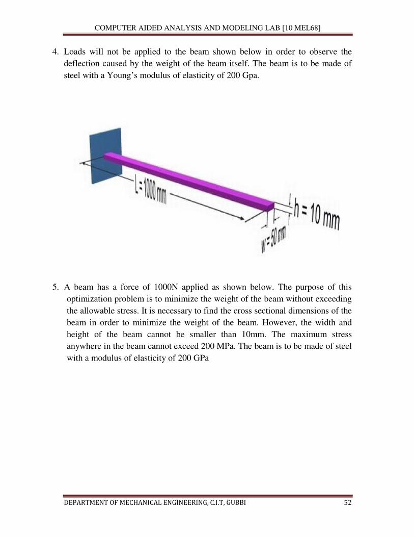
4. Loads will not be applied to the beam shown below in order to observe the
deflection caused by the weight of the beam itself. The beam is to be made of
steel with a Young’s modulus of elasticity of 200 Gpa.
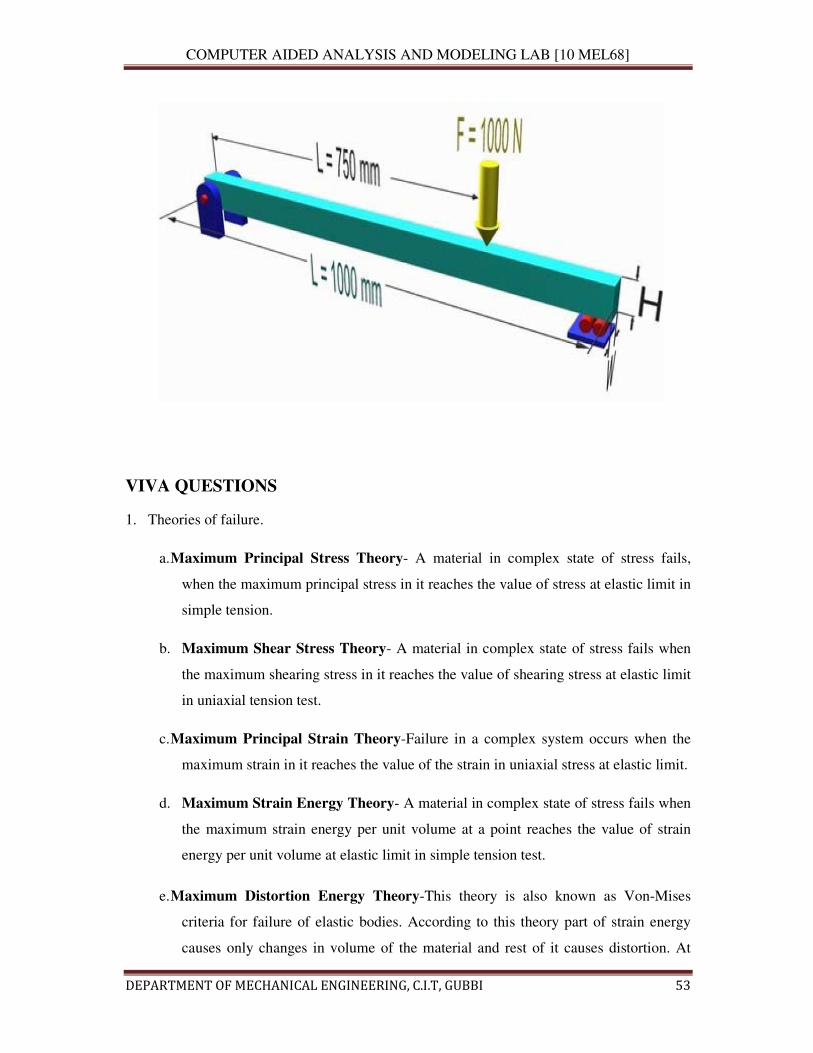
5. A beam has a force of 1000N applied as shown below. The purpose of this
optimization problem is to minimize the weight of the beam without exceeding
the allowable stress. It is necessary to find the cross sectional dimensions of the
beam in order to minimize the weight of the beam. However, the width and
height of the beam cannot be smaller than 10mm. The maximum stress
anywhere in the beam cannot exceed 200 MPa. The beam is to be made of steel
with a modulus of elasticity of 200 GPa
COMPUTER AIDED ANALYSIS AND MODELING LAB [10 MEL68]
DEPARTMENT OF MECHANICAL ENGINEERING, C.I.T, GUBBI 53
VIVA QUESTIONS
1. Theories of failure.
a. Maximum Principal Stress Theory- A material in complex state of stress fails,
when the maximum principal stress in it reaches the value of stress at elastic limit in
simple tension.
b. Maximum Shear Stress Theory- A material in complex state of stress fails when
the maximum shearing stress in it reaches the value of shearing stress at elastic limit
in uniaxial tension test.
c. Maximum Principal Strain Theory-Failure in a complex system occurs when the
maximum strain in it reaches the value of the strain in uniaxial stress at elastic limit.
d. Maximum Strain Energy Theory- A material in complex state of stress fails when
the maximum strain energy per unit volume at a point reaches the value of strain
energy per unit volume at elastic limit in simple tension test.
e. Maximum Distortion Energy Theory-This theory is also known as Von-Mises
criteria for failure of elastic bodies. According to this theory part of strain energy
causes only changes in volume of the material and rest of it causes distortion. At
COMPUTER AIDED ANALYSIS AND MODELING LAB [10 MEL68]
DEPARTMENT OF MECHANICAL ENGINEERING, C.I.T, GUBBI 54
failure the energy causing distortion per unit volume is equal to the distortion
energy per unit volume in uniaxial state of stress at elastic limit.
2. What is factor of safety?
The maximum stress to which any member is designed is much less than the ultimate
stress and this stress is called working stress. The ratio of ultimate stress to working stress
is called factor of safety.
3. What is Endurance limit?
The max stress at which even a billion reversal of stress cannot cause failure of the
material is called endurance limit.
4. Define: Modulus of rigidity, Bulk modulus
Modulus of rigidity: It is defined as the ratio of shearing stress to shearing strain within
elastic limit.
Bulk modulus:It is defined as the ratio of identical pressure ‘p’ acting in three mutually
perpendicular directions to corresponding volumetric strain.
5. What is proof resilience?
The maximum strain energy which can be stored by a body without undergoing
permanent deformation is called proof resilience.
6. What is shear force diagram?
A diagram in which ordinate represent shear force and abscissa represents the position of
the section is called SFD.
7. What is bending moment diagram?
A diagram in which ordinate represents bending moment and abscissa represents the
position of the section is called BMD.
8. Assumptions in simple theory of bending.
a. The beam is initially straight and every layer of it is free to expand or contract.
b. The material is homogeneous and isotropic.
COMPUTER AIDED ANALYSIS AND MODELING LAB [10 MEL68]
DEPARTMENT OF MECHANICAL ENGINEERING, C.I.T, GUBBI 55
c. Young’s modulus is same in tension and compression.
d. Stresses are within elastic limit.
e. Plane section remains plane even after bending.
f. The radius of curvature is large compared to depth of beam.
9. State the three phases of finite element method.
Preprocessing, Analysis & Post processing
10. What are the h and p versions of finite element method?
Both are used to improve the accuracy of the finite element method. In h version, the
order of polynomial approximation for all elements is kept constant and the numbers of
elements are increased. In p version, the numbers of elements are maintained constant and
the order of polynomial approximation of element is increased.
11. What is the difference between static analysis and dynamic analysis?
Static analysis: The solution of the problem does not vary with time is known as static
analysis.E.g.: stress analysis on a beam.
Dynamic analysis: The solution of the problem varies with time is known as dynamic
analysis.E.g.: vibration analysis problem.
12. What are Global coordinates?
The points in the entire structure are defined using coordinates system is known as global
coordinate system.
13. What are natural coordinates?A natural coordinate system is used to define any point
inside the element by a set of dimensionless number whose magnitude never exceeds
unity. This system is very useful in assembling of stiffness matrices.
14. What is a CST element?
Three node triangular elements are known as constant strain triangular element. It has 6
unknown degrees of freedom called u1, v1, u2, v2, u3, v3. The element is called CST
because it has constant strain throughout it.
15. Define shape function.
COMPUTER AIDED ANALYSIS AND MODELING LAB [10 MEL68]
DEPARTMENT OF MECHANICAL ENGINEERING, C.I.T, GUBBI 56
In finite element method, field variables within an element are generally expressed by the
following approximate relation:
Φ (x,y) = N1(x,y) Φ1+ N2(x,y) Φ2+N3(x,y) Φ3+N4(x,y) Φ4 where Φ1, Φ2, Φ3 and Φ4 are
the values of the field variables at the nodes and N1, N2, N3 and N4 are interpolation
function. N1, N2, N3, N4 are called shape functions because they are used to express the
geometry or shape of the element.
16. What are the characteristics of shape function?
The characteristics of the shape functions are as follows:
• The shape function has unit value at one nodal point and zero value at the other
nodes.
• The sum of shape functions is equal to one.
17. Why polynomials are generally used as shape function?
• Differentiation and integration of polynomials are quite easy.
• The accuracy of the results can be improved by increasing the order of the
polynomial.
• It is easy to formulate and computerize the finite element equations.
18. State the properties of a stiffness matrix.
The properties of the stiffness matrix [K] are:
• It is a symmetric matrix.
• The sum of the elements in any column must be equal to zero.
• It is an unstable element, so the determinant is equal to zero.
19. What are the difference between boundary value problem and initial value problem?
The solution of differential equation obtained for physical problems which satisfies some
specified conditions known as boundary conditions. If the solution of differential
equation is obtained together with initial conditions then it is known as initial value
COMPUTER AIDED ANALYSIS AND MODELING LAB [10 MEL68]
DEPARTMENT OF MECHANICAL ENGINEERING, C.I.T, GUBBI 57
problem. If the solution of differential equation is obtained together with boundary
conditions then it is known as boundary value problem.
20. What is meant by plane stress?
Plane stress is defined as a state of stress in which the normal stress (α) and the shear
stress directed perpendicular to plane are zero.
21. Define plane strain.
Plane strain is defined to be a state of strain in which the strain normal to the xy plane
and the shear strains are assumed to be zero.
22. Define Quasi-static response.
When the excitations are varying slowly with time then it is called quasi-static response.
23. What is a sub parametric element?
If the number of nodes used for defining the geometry is less than the number of nodes
used for defining the displacements is known as sub parametric element.
24. What is a super parametric element?
If the number of nodes used for defining the geometry is more than the number of nodes
used for defining the displacements is known as sub parametric element.
25. What is meant by isoparametric element?
If the number of nodes used for defining the geometry is same as number of nodes used
for defining the displacements then it is called parametric element.
26. What is the purpose of isoparametric element?
It is difficult to represent the curved boundaries by straight edges finite elements. A large
number of finite elements may be used to obtain reasonable resemblance between
original body and assemblage. In order to overcome this drawback, iso parametric
elements are used i.e for problems involving curved boundaries, a family of elements
‘isoparametric elements’ are used.
COMPUTER AIDED ANALYSIS AND MODELING LAB [10 MEL68]
DEPARTMENT OF MECHANICAL ENGINEERING, C.I.T, GUBBI 58
27. What are isotropic and orthotropic materials?
A material is isotropic if its mechanical and thermal properties are the same in all
directions. Isotropic materials can have homogeneous or non-homogeneous microscopic
structures.
Orthotropic materials:A material is orthotropic if its mechanical or thermal properties are
unique and independent in three mutually perpendicular directions.
28. What is discretization?
Discretization is the process of dividing given problem into several small
elements, connected with nodes.
29. Steps in FEM
• Discretization
• Selection of the displacement models
• Deriving element stiffness matrices
• Assembly of overall equations/ matrices
• Solution for unknown displacements
• Computations for the strains/stresses