Labor Immobility and Exchange Rate Regimes: An alternative Explanation for the Fall of the Interwar Gold Exchange Standard David Khoudour-Castéras [email protected]Universidad Externado de Colombia May 2006 Abstract Beyond the respective functioning of the classical gold standard and the interwar gold exchange standard, one of the main differences between both periods lay on the degree of labor mobility. While the pre-1914 world was characterized by massive migration flows, the interwar years were marked by a dramatic fall in labor movements, owing to the adoption of restrictive immigration policies in the main receiving countries and the implementation of social safety nets in several western and northern European countries. As a result, labor mobility could not play anymore the role of adjustment mechanism that it had during the classical gold standard. Indeed, the existence of a number of adjustment constraints, including wage rigidities and factor immobility, led the countries with fixed exchange rates to adopt counterproductive adjustment mechanisms, such as trade protectionism, that resulted in both internal and external imbalances. Against this background, the return to flexible exchange rates was the only credible option. JEL Classification: F22, F33, N10 Keywords: Gold Exchange Standard, International Adjustment, Labor Mobility
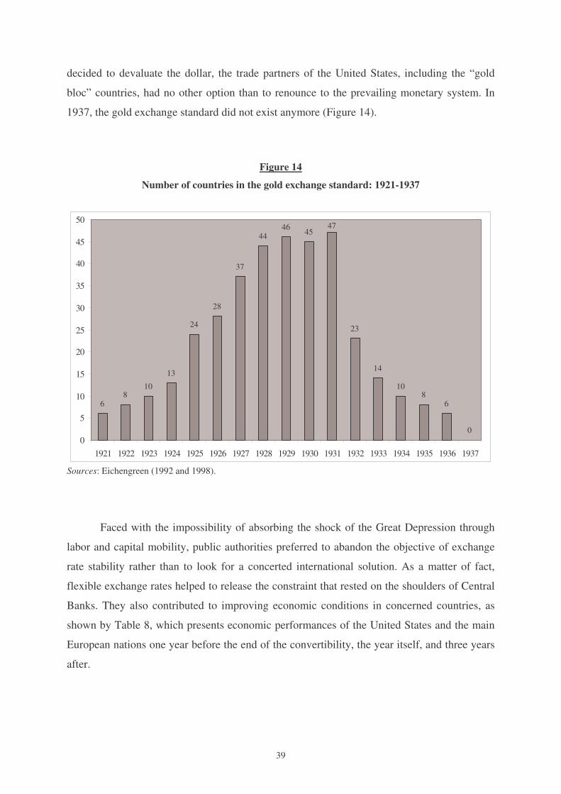
Transcript
Labor Immobility and Exchange Rate Regimes:
An alternative Explanation for the Fall of the Interwar Gold
Beyond the respective functioning of the classical gold standard and the interwar gold exchange standard, one of the main differences between both periods lay on the degree of labor mobility. While the pre-1914 world was characterized by massive migration flows, the interwar years were marked by a dramatic fall in labor movements, owing to the adoption of restrictive immigration policies in the main receiving countries and the implementation of social safety nets in several western and northern European countries. As a result, labor mobility could not play anymore the role of adjustment mechanism that it had during the classical gold standard. Indeed, the existence of a number of adjustment constraints, including wage rigidities and factor immobility, led the countries with fixed exchange rates to adopt counterproductive adjustment mechanisms, such as trade protectionism, that resulted in both internal and external imbalances. Against this background, the return to flexible exchange rates was the only credible option. JEL Classification: F22, F33, N10 Keywords: Gold Exchange Standard, International Adjustment, Labor Mobility
1
Labor Immobility and Exchange Rate Regimes: An alternative Explanation
for the Fall of the Interwar Gold Exchange Standard
“It is easy to sum up the conventional wisdom that quickly emerged in response to the problems of the global economy. Everything that was moving across national boundaries – whether capital, goods, or people – really had no business to be doing that and should be stopped. If it could not be stopped, it should be controlled, in accordance with a definition of national interest.”
Harold James (2001: 187)
Introduction
The two decades that separated the First from the Second World War are also known
as the period of the “end of the globalization” (James, 2001): trade flows significantly slowed
down in comparison with the pre-war years, capital mobility was strongly constrained,
barriers to international labor mobility increased, and all the attempts to stabilize currencies
failed. Even though the 1929 crash and the Great Depression that followed it sparked off the
globalization backlash, they are not the only responsible. The adoption, during the 1920s, of
several protectionist measures probably induced – and sped up – the crisis of the 1930s, while
the widespread renunciation of fixed exchange rates after 1931 was in keeping with the non-
cooperative policies at that time. In that sense, the international trade and monetary
cooperation that marked the classical gold standard period was replaced by a logic of strong
economic nationalism
In fact, the protectionist temptation, which went well beyond trade measures, appeared
with the first significant restrictions on immigration put into place in the United States at the
beginning of the 1920s. Such border controls marked a turning point compared to the pre-war
years, characterized by massive population movements between the European countries and
the New World. It is also likely that they contributed, at least indirectly, to the fall of the gold
standard, or more precisely of the gold exchange standard adopted during the 1922 Genoa
conference. Indeed, maintaining fixed exchange rate regimes implies the existence of a
number of adjustment mechanisms – more or less automatic – that enables to offset, in the
event of disequilibria, exchange rate rigidity. Labor mobility, as shown by Mundell (1961),
plays an important role in this adjustment process.
2
In that regard, the classical gold standard period represents a perfect illustration of the
importance of migration flows in the success of fixed exchange rate regimes. At that time,
international migration was free and the countries that chose to peg their currency to gold
could transfer the adjustment burden on labor mobility (Khoudour-Castéras, 2005a). To the
contrary, the gold exchange standard had to face a number of constraints that seriously limited
adjustment possibilities. In addition to the hindrances to workers’ mobility, the interwar
period was also different from the gold standard years on account of an environment of higher
wage rigidities and lower capital mobility. Therefore, the costs of maintaining the exchange
rate stability were high, which explains that, confronted with the Great Depression of the
1930s, most of the nations that joined the Genoa International Monetary System opted for the
abandon of fixed exchange rates and the return to monetary policy autonomy.
In order to show how the end of labor mobility could have been at the origin of the fall
of the gold exchange standard, the remainder of the paper is organized as follows. First,
Section I presents the evolution of international migration policies. The goal is notably to
understand the mechanisms that led the United States as well as most of the countries that
were traditionally open to immigration to implement restrictive measures. Then, Section II
underscores the fact that the contraction of migration flows after World War I was not only
due to the barriers that immigration countries put into place, but also to specific changes in the
European nations that entailed a reduction in labor exports. This section emphasizes in
particular the impact of social policies on the slowdown in European emigration. Next,
Section III shows that the decrease in international migration brought about a disconnection
between business cycles and migration movements, that is, that labor mobility could not play
anymore its role of adjustment mechanism. Lastly, Section IV tries to establish how the lack
of labor mobility could have been harmful to the gold exchange standard: the existence of a
number of adjustment constraints, including wage rigidities and factor immobility, led the
countries with fixed exchange rates to adopt counterproductive adjustment mechanisms, such
as trade protectionism, that resulted in both internal and external imbalances. Against this
background, retiring from the gold exchange standard was the only credible option.
I – The Implementation of Restrictive Immigration Policies
The pass-through from a world with free labor mobility to a closed world did not
occur suddenly: “Contrary to the conventional wisdom, there was not one big regime switch
around World War I from free (and often subsidized) immigration to quotas, but rather an
3
evolution toward more restrictive immigration policy in the New World. Attitudes changed
slowly and over a number of decades rather than all at once.” (O’Rourke and Williamson,
1999: 186). Yet, the most drastic measures were adopted during the interwar years, putting an
end to the mass migration phenomenon that characterized the pre-1914 era. Under the double
pressure of trade unions and political movements, most of the receiving countries closed their
door to migrants. What is remarkable in this process is that it chiefly cropped up before the
Great Depression, that is, in a context of relatively good economic health.
Protectionist temptation and nativist influence in the United States
American trade union organizations played a driving role in the process that led to the
adoption of restrictive measures against foreign workers: "The nationalisation of labour
unions, that is their growth and institutionalisation in a national, and even international
(many of them included Canadian branches) dimension, provided a new scale of intervention.
[...] They came to define what was the American standard of wages, and by the same token
also imposed a national vision of the American workers' life style. They also established
centralised decision-making and bureaucratic structures that placed them in a position to
create a broad movement and publicise their demands." (Collomp, 2003: 240). It was in this
context that first waves of protest against foreign labor appeared. Initially confined to the
West Coast, they targeted Chinese workers. These arrived at the time of the Gold Rush and
were used for laborious work in the fields or the mines, and rail laying operations. When the
building of the transcontinental railways ended, a large number of them moved to San
Francisco, where they were considered as rivals by local active population. Discriminatory
measures and riots against Chinese increased, all the more because some of them were used as
strike breakers by the manufacturers.
Then, it was the turn of the Japanese to face the fire of criticism and to suffer riots.
Like the Chinese, they were employed to do the badly paid jobs. Hence the creation in 1905,
by American trade unions, of the Japanese and Korean Exclusion League, whose goal was to
stop the immigration of persons who accepted to work for wages that were considered as too
low. Afterwards, the “new migrants” from central and southern Europe were accused of
putting downward pressure on American wages. Unskilled workers were especially targeted:
“The pressure to stop immigration had little to do with the war. It was a result of the surge of
immigration in 1900-1910, which had a discernible impact on the wages of less skilled
workers.” (James, 2001: 173). This affirmation is partly confirmed by Williamson (1996),
4
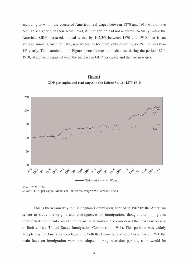
according to whom the course of American real wages between 1870 and 1910 would have
been 15% higher than their actual level, if immigration had not occurred. Actually, while the
American GDP increased, in real terms, by 102.3% between 1870 and 1910, that is, an
average annual growth of 1.8%, real wages, as for them, only raised by 47.3%, i.e. less than
1% yearly. The examination of Figure 1 corroborates the existence, during the period 1870-
1910, of a growing gap between the increase in GDP per capita and the rise in wages.
Figure 1
GDP per capita and real wages in the United States: 1870-1910
147,3
202.3
0
50
100
150
200
250
1870
1872
1874
1876
1878
1880
1882
1884
1886
1888
1890
1892
1894
1896
1898
1900
1902
1904
1906
1908
1910
GDP/capita Wages
Note: 1870 = 100. Sources: GDP per capita: Maddison (2003); real wages: Williamson (1995).
This is the reason why the Dillingham Commission, formed in 1907 by the American
senate to study the origins and consequences of immigration, thought that immigrants
represented significant competition for national workers and considered that it was necessary
to limit entries (United States Immigration Commission, 1911). This position was widely
accepted by the American society, and by both the Democrat and Republican parties. Yet, the
main laws on immigration were not adopted during recession periods, as it would be
5
expected, but rather during the growing years that followed World War I, which indicates that
the protection of American workers was not the sole motive for refusing admission to
immigrants.
Thus, nativism was a political movement that advocated for a racial view of America
and, therefore, opposed immigration, in particular migration proceeding from “non-Nordic”
countries. This opposition to the American melting pot began to develop about the middle of
the nineteenth century, with the creation of several political parties (Native American Party,
Know Nothing, Order of the Sprangled Banner…) engaged in a desperate struggle against the
Irish “papists”, who arrived in large numbers after the famine that ravaged their country.
Then, the xenophobic agitation, especially on the West Coast, focused on the Chinese and
Japanese, whose customs appeared to represent a social threat, and who seemed unable to
integrate into the American society. In parallel with this opposition to Asian immigration,
“new migrants”, from western and southern Europe, were stigmatized by the “old migrants”
who came, as for them, from western and northern Europe.
American employers and politicians especially dreaded the spread of extreme left
ideas. In that sense, the 1886 Haymarket affair1 in Chicago marked the starting point of an
important wave of repression against “anarchists”, which were associated with the Jews
proceeding from eastern Europe. Restrictions against Jews were hence enacted in some
professions as well as in universities. After the October Revolution in Russia, the “Red Scare”
quickly expanded, and the arrests and deportations of foreigners increased. World War I also
contributed to strengthen the feeling of external threat, in particular from Americans of
German extraction, and gave rise to a strong Americanization movement that brought about,
for instance, the spread of English classes for immigrants.
It was in this context that the Immigration Restriction League, established in 1894 to
provide a political platform for theories on the superiority of the Nordic races, undertook,
along with the Ku Klux Klan, an active campaign against mass immigration. Most of the
American legislation on border controls actually followed from this activism, and all means
were good to exclude undesirable people: literacy tests, entry quotas, laws against the
anarchists or the poor… The twentieth century definitely meant the end of mass migration to
the United States.
1 While Chicago workers had been demonstrating since may 1st in favor of the eight-hour day, and had been violently opposed to the police, a bomb exploded in the middle of the policemen in Haymarket Square, on May 4, 1886. The police answered by shooting at the crowd, killing seven or eight demonstrators and wounding about a hundred of persons. Seven anarchists, most of them of German extraction, were sentenced to death, even though there was no proof of their implication in the attack.
6
American laws on immigration
The first restrictive law on immigration was enacted in 1882. The Chinese community
was specifically concerned since the Chinese Exclusion Act, initially enacted for a ten-year
period and then renewed in 1892, made the immigration of Chinese workers illegal. They
were also denied American citizenship, which did not allow them to have access to a number
of reserved jobs. Then, the Japanese were targeted: “So long as the Japanese remained
willing to perform agricultural labor at low wages, they remained popular with California
ranchers. But… many Japanese began to lease and buy agricultural land for farming on their
own account. This enterprise has the two-fold result of creating Japanese competition in the
produce field and decreasing the number of Japanese farmhands available.” (Light, 1972: 9).
American and Japanese governments adopted in 1907 a gentlemen’s agreement aiming at the
limitation of Japanese immigration in the United States. Moreover, several western States,
including California, restricted Japanese land acquisition.
Besides these racial measures, several individual categories were denied access to the
American territory. From 1882, lunatics and the mentally handicapped were concerned by
these restrictions. Next, an 1891 act excluded carriers of contagious or pestilential diseases,
polygamists and the destitute, while a 1903 act tackled beggars, prostitutes, epileptics, and
above all anarchists, especially feared since the assassination, two years earlier, of President
Mc Kinley by Leon Czolgoz. Another act of 1907 referred to criminals and tubercular
patients. The same year, children below sixteen years old not accompanied by one of their
parents were also denied access to the United States in order to try to put an end to child
labor.
But it was really after World War I that the fight against immigration took on new
dimensions. In 1917, after many fruitless attempts and despite President Wilson’s veto, the
literacy test was finally adopted: all the foreigners who wished for settling in the United States
had to demonstrate that they were able to read between thirty and eighty words, in the
language of their choice. Furthermore, new migrants had to pay an eight-dollar tax. The 1917
legislation mainly targeted citizens from eastern and southern Europe, where literacy rates
were low and poverty was high. Then, in 1921, the first act on quotas was enacted and
immigration became a function of the previous settlement of national communities on the
American soil: only 3% of the number of nationals already established in the United States
during the 1910 census could enter. Moreover, from 1922, the candidates to immigration had
7
to pay nine dollars to obtain a visa (which had to be added to the 1917 tax). But these
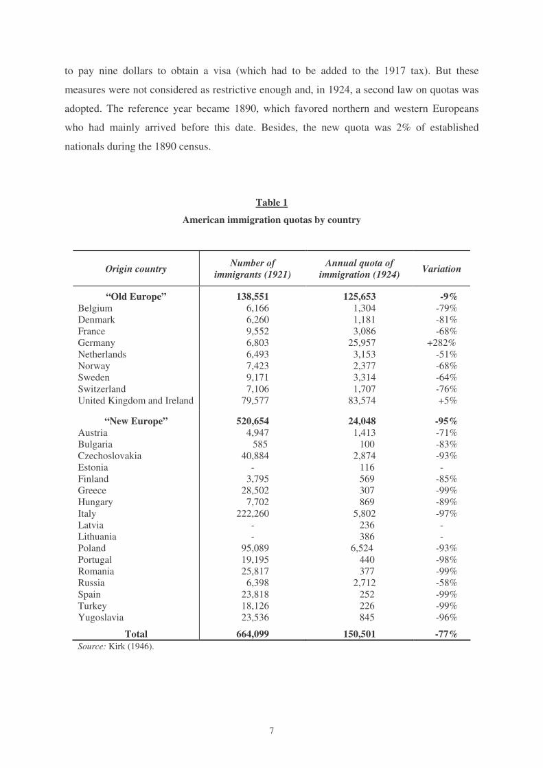
measures were not considered as restrictive enough and, in 1924, a second law on quotas was
adopted. The reference year became 1890, which favored northern and western Europeans
who had mainly arrived before this date. Besides, the new quota was 2% of established
nationals during the 1890 census.
Table 1
American immigration quotas by country
Origin country Number of immigrants (1921)
Annual quota of immigration (1924) Variation
“Old Europe” Belgium Denmark France Germany Netherlands Norway Sweden Switzerland United Kingdom and Ireland
“New Europe” Austria Bulgaria Czechoslovakia Estonia Finland Greece Hungary Italy Latvia Lithuania Poland Portugal Romania Russia Spain Turkey Yugoslavia
With the notable exception of Germany, the United Kingdom and Ireland, which
benefited from the quota legislation, most of the European countries were affected by the
1924 quotas (Table 1). Logically, countries with recent emigration to the United States, that
is, eastern and southern European countries, were particularly hard hit by the implementation
of these quantitative restrictions. On the contrary, the changes did not affect Latin-American
workers who, like their Canadian counterpart, were not subject to the quota laws. Indeed,
landowners of southwestern American States, who started to use Mexican labor force during
the first world conflict, opposed them. Furthermore, such a preferential treatment was in
keeping with the political logic of pan-Americanism: The restrictive immigration laws […]
were essentially an expression of American revulsion from the Old World; and since, as a
consequence of its isolationism, the United States tended to draw closer to other American
countries, it was natural to place immigration from them upon a special footing.” (Jones,
1992: 248). Yet, the so-called “good neighborhood” policy did not prevent the United States
from implementing, in 1924, a border police along the Rio Grande in order to stop illegal
immigration from Mexico (Mariage-Strauss, 2002).
With the beginning of the Great Depression, controls became stricter. The financial
standing of immigrants was deeply analyzed and American consulates were in charge of
medical visits in sending countries. Besides, close relations had to commit themselves, if
necessary, to financially help the immigrant. Finally, with the crisis, a great number of
workers were denied the right to practice their profession in the US, inter alia lawyers,
doctors and teachers (Jones, 1992).
The worldwide extension of border controls
As in the United States, the first restrictive measures adopted by Canada and Australia
in terms of immigration targeted Asian populations. Thus, in 1885, the Canadian Parliament
introduced a lump sum tax of fifty dollars for all Chinese immigrants. In 1900, the amount of
the tax came to one hundred dollars, then five hundred dollars in 1905 (Daniels, 1995). In
other respects, Canadian authorities promulgated a decree, in 1908, forbidding the entry on its
territory of every immigrant who had put into port during her arrival journey. Without saying
it, this decision was directed at Indian immigrants who, due to the lack of a direct shipping
line between India and Canada, was forced to transfer through Japan or Hong Kong to go to
Canada (Buchignani and al., 1985). Australia, as for it, enacted in 1901 a law aiming at
limiting the entry of Asian immigrants through a literacy test: when immigration agents
9
required it, candidates for migration had to take a dictation test of fifty words, but only in a
European language (Markus, 1979).
In a general way, measures adopted before 1914 did not affect European immigration,
even though British colonies tended to privilege immigrants proceeding from Great Britain.
On the contrary, the nationalism that followed World War I, combined with the economic
problems of the interwar period, brought about the strengthening of border controls in most of
the immigration countries. Thus, in 1923, Canada enacted a law that formally banned Chinese
immigration. Then, in 1933, Canadian authorities decided to limit the entry of southern and
eastern Europeans, who only could have access to farm and domestic work (James, 2001). On
the other hand, natives from Belgium, Denmark, France, Germany, Netherlands, Sweden and
Switzerland belonged to the “preferred countries” list and had the same advantages than
British subjects. In the same way, Australia promulgated in 1925 a law that restricted the
entry of non-British migrants into its territory, through the adoption of citizenship and
occupation criteria. The Queensland Province went farer, by forbidding foreigners to buy
lands or to work in certain industries (de Lepervanche, 1975). Such policies reflect the
atmosphere at the time against immigrants, in particular these coming from southern Europe:
“Southern Europeans who came to Australia in the 1920s were treated with suspicion.
Immigrant ships were refused permission to land and there were ‘anti-Dago’ riots in the
1930s.” (Castles and Miller, 1998: 62).
Faced with the upsurge of border controls in Anglo-Saxon countries, candidates for
migration headed for Latin America. Thus, although not reaching the pre-war levels, the
immigration volume remained high in Argentina: 140,000 immigrants on annual average
during the decade 1921-1930 as against 177,000 between 1901 and 1910 (239,000 during the
decade 1904-1913). Brazil, as for it, received more immigrants after World War I (84,000
entries on annual average during the decade 1921-1930) than during the decade 1901-1910
(70,000 entries). Mexico and Uruguay also drew a larger number of immigrants during the
1920s (46,000 and 17,000 average entries, respectively, for Mexico and Uruguay during the
decade 1921-1930) than at the beginning of the century (respectively, 40,000 and 11,000
entries for the period 1904-1913).
Similarly, the few European nations open to immigration became more attractive as
the rest of the world closed its doors. Eastern and southern Europeans, in particular, for whom
it had become difficult to move overseas, opted for Belgium or France. The latter recorded a
migratory net balance of about two millions of persons during the 1920s, whereas it was only
250,000 during the decade 1900-1910 (Bairoch, 1997). At the end of the decade, France
10
hence succeeded the United States as the main receiving countries in terms of European
migration. A private institution, the Société Générale d’Immigration (SGI), was in charge of
recruiting abroad, mainly for the farming and mining sectors, and of establishing contracts
between foreign workers and domestic firms (Castles et Miller, 1998). Belgium, as for it,
received about 140,000 foreigners during the 1920s. Italians and Polish, followed by
Spaniards and, in a lesser extent, by Portuguese, Czechoslovaks and Yugoslavs represented
most of the migrants within the European continent (Kirk, 1946).
But, the 1930s crisis gave rise to a new series of border control policies that put a
definitive end to the free movement of persons on a worldwide scale. Thus, in 1930, South
Africa decided to ban the entry on its territory to the citizens coming from the “non-preferred”
countries, that is, the non-Anglo-Saxon ones. Latin America countries, particularly affected
by the shock wave of the Great Depression, also decided to restrict immigration, while
European nations began to strengthen their own migration policy. Switzerland, for instance,
began to require, after 1932, that the candidates for immigration fulfill several financial
conditions. The same year, France implemented a quota system with the goal of reducing the
number of foreign workers in French firms. Afterwards, French government authorized the
layoffs of immigrants in sectors affected by the crisis and chose to deport part of them (Weil,
1991). Hitler’s Germany, as for it, adopted a strict border control policy by limiting
recruitment possibilities of foreign workers, by opting for the “national preference” in terms
of employment, by punishing the firms that resorted to clandestine work, and finally, by
deporting the undesirable foreigners (Dohse, 1981).
Finally, it is noteworthy that after World War I, several countries put into place exit
control measures. Former Soviet Union, for instance, expressly prohibited, with some
exceptions, emigration of its nationals. In the same way, Mussolini’s Italy tried to control
migration outflows by giving permission to expatriate only to labor contract holders or to the
persons who could be hosted by a close relative.
II –The Impact of Social Policies on European emigration
Although the increase in worldwide border controls was largely accountable for the
decrease in European emigration, it was not the only responsible for it. As a matter of fact, the
quota system adopted by the United States in the 1920s played a great part in the reduction of
inflows from Europe. Yet, during the 1930s, not one of the European nations, not even the
southern and eastern ones, fulfilled its quota: “In the decade of the 1930s, the quotas became
11
non-binding. From 1930 to 1931, quota immigration dropped by 62 percent. In 1933 only
8,220 quota immigrants out of a permissible total of 153,879 were admitted. No immigrant
category fulfilled its quota for any year in the decade. Southern and eastern European nations
did reach nearly 90 percent of their quota, but only in one year, 1939, as refugee emigrants
fled Europe. No other sources reached more than 41 percent of their quotas.” (Gemery, 1994:
180). It seems therefore necessary to look for the internal determinants of the European
emigration decline. It that sense, the introduction of an embryonic Welfare State in several
European nations might have contributed to the decrease in emigration.
The internal determinants of the European emigration slowdown
First and foremost, international migration flows were interrupted by World War I.
European armies had overwhelming needs of “cannon fodder” and about 8.6 million soldiers
and 6 million civilians were killed during the war (Bairoch, 1997). Besides, 1918 and 1919
were marked by an epidemic of “Spanish flu”, which is estimated to have taken more than 20
million lives all over the world (ibid). The potential number of migrants was thereby affected
for many years. But, beyond this double demographic catastrophe, there was a long-term
trend of decrease in the population growth, related to the demographic transition in most of
the European countries. As a matter of fact, despite an upturn in the post-war birth rate, the
1920s and 1930s were characterized by a natural growth rate of the European population
below its pre-1914 level and above all its nineteenth century level (Kirk, 1946). In northern
and western European countries, notably, demographic growth rates fell rapidly, while the
impulse continued to be high in southern and eastern nations. This difference in demographic
behavior partly explains why migration candidates during the interwar years were more
numerous in the latter countries. In addition to these demographic changes, the economic
progress in European countries played a significant role. Employment opportunities increased
as towns developed and trade and industry grew, while European labor markets contracted
under the influence of the war and the slowdown in demographic growth. As a result, the
wage convergence process initiated before World War I should have increased after the
conflict. However, wage differentials remained high during the interwar years, at least
between Europe and the United States.
12
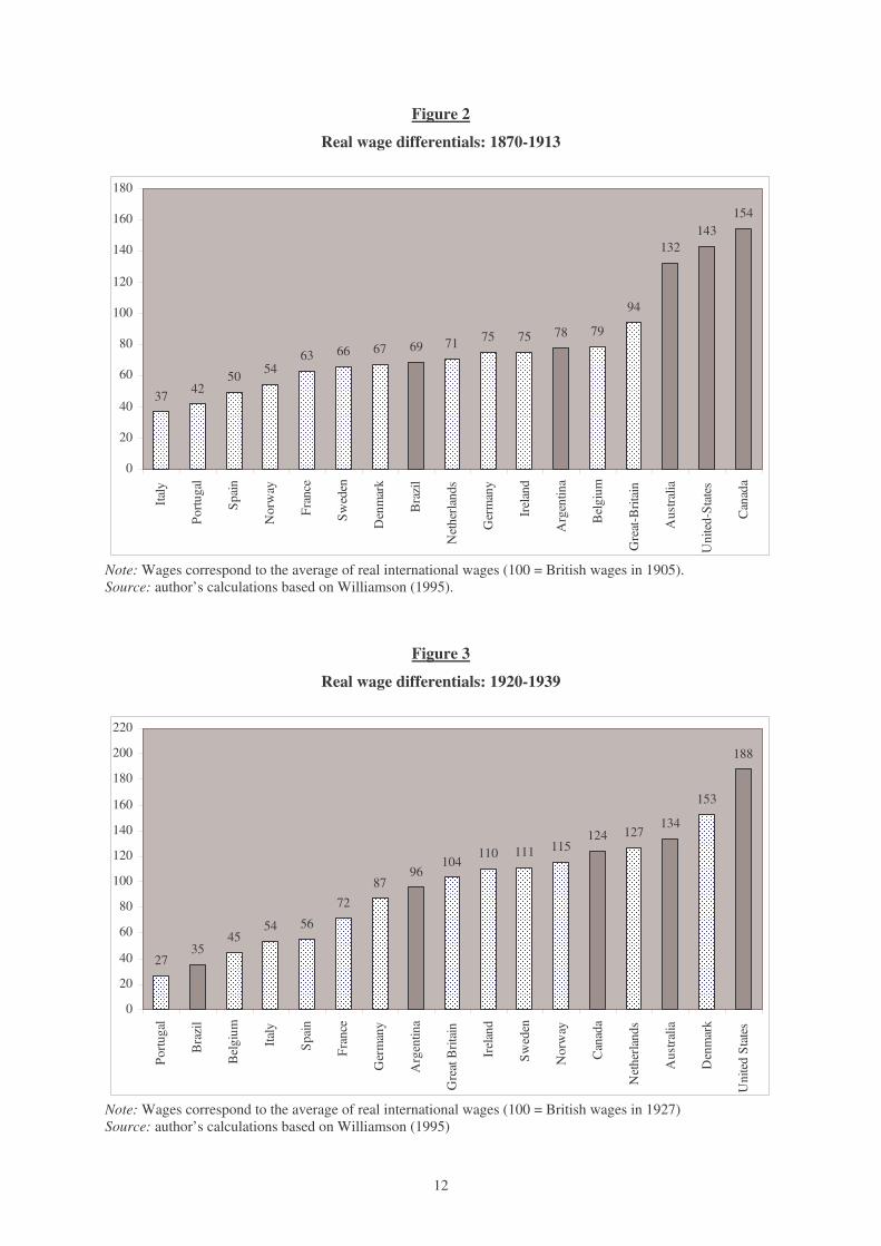
Figure 2
Real wage differentials: 1870-1913
37
6371
78
143154
132
94
797575696766
545042
0
20
40
60
80
100
120
140
160
180
Italy
Portu
gal
Spai
n
Nor
way
Fran
ce
Swed
en
Den
mar
k
Bra
zil
Net
herla
nds
Ger
man
y
Irel
and
Arg
entin
a
Bel
gium
Gre
at-B
ritai
n
Aus
tralia
Uni
ted-
Stat
es
Can
ada
Note: Wages correspond to the average of real international wages (100 = British wages in 1905). Source: author’s calculations based on Williamson (1995).
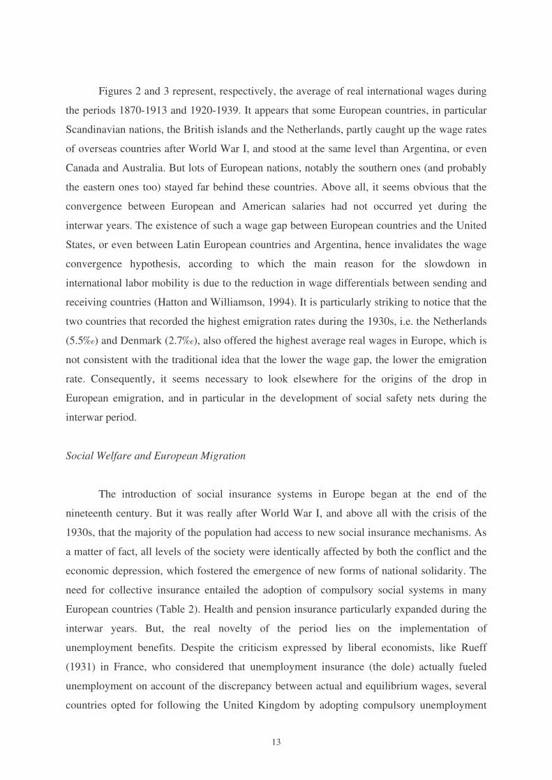
Figure 3
Real wage differentials: 1920-1939
2735
4554 56
7287
96104
110 111 115124 127
134
153
188
0
20
40
60
80
100
120
140
160
180
200
220
Portu
gal
Bra
zil
Bel
gium
Italy
Spai
n
Fran
ce
Ger
man
y
Arg
entin
a
Gre
at B
ritai
n
Irel
and
Swed
en
Nor
way
Can
ada
Net
herla
nds
Aus
tralia
Den
mar
k
Uni
ted
Stat
es
Note: Wages correspond to the average of real international wages (100 = British wages in 1927) Source: author’s calculations based on Williamson (1995)
13
Figures 2 and 3 represent, respectively, the average of real international wages during
the periods 1870-1913 and 1920-1939. It appears that some European countries, in particular
Scandinavian nations, the British islands and the Netherlands, partly caught up the wage rates
of overseas countries after World War I, and stood at the same level than Argentina, or even
Canada and Australia. But lots of European nations, notably the southern ones (and probably
the eastern ones too) stayed far behind these countries. Above all, it seems obvious that the
convergence between European and American salaries had not occurred yet during the
interwar years. The existence of such a wage gap between European countries and the United
States, or even between Latin European countries and Argentina, hence invalidates the wage
convergence hypothesis, according to which the main reason for the slowdown in
international labor mobility is due to the reduction in wage differentials between sending and
receiving countries (Hatton and Williamson, 1994). It is particularly striking to notice that the
two countries that recorded the highest emigration rates during the 1930s, i.e. the Netherlands
(5.5‰) and Denmark (2.7‰), also offered the highest average real wages in Europe, which is
not consistent with the traditional idea that the lower the wage gap, the lower the emigration
rate. Consequently, it seems necessary to look elsewhere for the origins of the drop in
European emigration, and in particular in the development of social safety nets during the
interwar period.
Social Welfare and European Migration
The introduction of social insurance systems in Europe began at the end of the
nineteenth century. But it was really after World War I, and above all with the crisis of the
1930s, that the majority of the population had access to new social insurance mechanisms. As
a matter of fact, all levels of the society were identically affected by both the conflict and the
economic depression, which fostered the emergence of new forms of national solidarity. The
need for collective insurance entailed the adoption of compulsory social systems in many
European countries (Table 2). Health and pension insurance particularly expanded during the
interwar years. But, the real novelty of the period lies on the implementation of
unemployment benefits. Despite the criticism expressed by liberal economists, like Rueff
(1931) in France, who considered that unemployment insurance (the dole) actually fueled
unemployment on account of the discrepancy between actual and equilibrium wages, several
countries opted for following the United Kingdom by adopting compulsory unemployment
14
insurance. The result was that at the dawn of World War II, around half the European
employees benefited from old age and unemployment insurance (Flora and Alber, 1981).
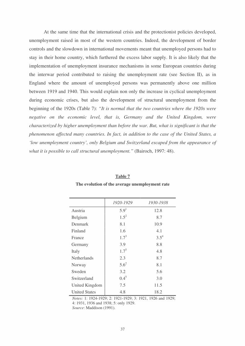
Table 2
The implementation of social insurance mechanisms in Europe before World War II
Industrial accident insurance
Health insurance
Pension insurance
Unemployment insurance
Austria 1887 1888 1927 1920
Belgium (1903) (1894) 1924 (1900) (1920)
Denmark 1916 (1898)
1933 (1892)
1921/1922 (1891) (1907)
Finland 1895 / 1937 (1917)
France (1898) 1930 (1898)
1910 (1895) (1905)
Germany 1884 (1871) 1833 1889 1927
Italy 1898 1928 (1886)
1919 (1898) 1919
Netherlands 1901 1929 1913 (1916)
Norway 1894 1909 1936 1938 (1906)
Sweden 1916 (1901) (1891) 1913 (1934)
Switzerland 1911 (1881) (1891) / (1924)
United Kingdom (1897) 1911 1925 (1908) 1911
Note: The numbers in parentheses refer to subsidized voluntary insurance; the other numbers correspond to compulsory insurance. The interwar years are in bold. Source: Flora (1983).
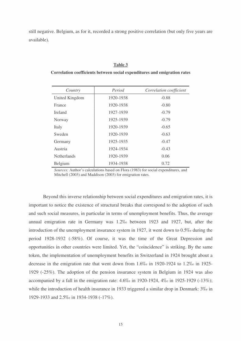
The question now is to know to what extent the development of social policies had an
influence on the course of European emigration after World War I. Thus, Table 3 shows that
there was a strong negative correlation between social expenditures as a percentage of GDP
and emigration rates in at least six countries (the United Kingdom, France, Ireland, Norway,
Italy and Sweden); the correlation was less significant for Germany and Austria, but it was
15
still negative. Belgium, as for it, recorded a strong positive correlation (but only five years are
available).
Table 3
Correlation coefficients between social expenditures and emigration rates
Country Period Correlation coefficient
United Kingdom 1920-1938 -0.88
France 1920-1938 -0.80
Ireland 1927-1939 -0.79
Norway 1925-1939 -0.79
Italy 1920-1939 -0.65
Sweden 1920-1939 -0.63
Germany 1925-1935 -0.47
Austria 1924-1934 -0.43
Netherlands 1920-1939 0.06
Belgium 1934-1938 0.72 Sources: Author’s calculations based on Flora (1983) for social expenditures, and Mitchell (2003) and Maddison (2003) for emigration rates.
Beyond this inverse relationship between social expenditures and emigration rates, it is
important to notice the existence of structural breaks that correspond to the adoption of such
and such social measures, in particular in terms of unemployment benefits. Thus, the average
annual emigration rate in Germany was 1.2‰ between 1923 and 1927, but, after the
introduction of the unemployment insurance system in 1927, it went down to 0.5‰ during the
period 1928-1932 (-58%). Of course, it was the time of the Great Depression and
opportunities in other countries were limited. Yet, the “coincidence” is striking. By the same
token, the implementation of unemployment benefits in Switzerland in 1924 brought about a
decrease in the emigration rate that went down from 1.6‰ in 1920-1924 to 1.2‰ in 1925-
1929 (-25%). The adoption of the pension insurance system in Belgium in 1924 was also
accompanied by a fall in the emigration rate: 4.6‰ in 1920-1924, 4‰ in 1925-1929 (-13%);
while the introduction of health insurance in 1933 triggered a similar drop in Denmark: 3‰ in
1929-1933 and 2.5‰ in 1934-1938 (-17%).
16
Figure 4
Social expenditures and emigration rates in Europe: 1920-1939
Belgium
AustriaGermany
Sweden
United Kingdom
Norway
Italy
Netherlands
Denmark
SwitzerlandFrance
-1
0
1
2
3
4
5
6
7
0 2 4 6 8 10 12 14
Social expenditures/GDP (%)
Em
igra
tion
rat
e (‰
)
Notes: Horizontal axis represents the average of social expenditures as a percentage of GDP; vertical axis corresponds to the average of emigration rates. Periods for each country are the same than in Table 3. There are only data for two years in Denmark (1929 and 1938) and one year in Switzerland (1938). The correlation coefficient is -0.54. Sources: Author’s calculations based on Flora (1983) for social expenditures, and Mitchell (2003) and Maddison (2003) for emigration rates.
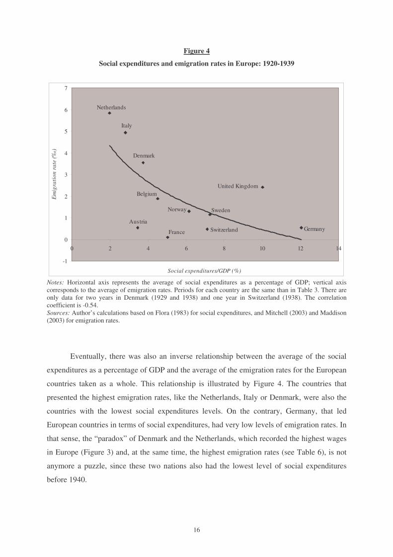
Eventually, there was also an inverse relationship between the average of the social
expenditures as a percentage of GDP and the average of the emigration rates for the European
countries taken as a whole. This relationship is illustrated by Figure 4. The countries that
presented the highest emigration rates, like the Netherlands, Italy or Denmark, were also the
countries with the lowest social expenditures levels. On the contrary, Germany, that led
European countries in terms of social expenditures, had very low levels of emigration rates. In
that sense, the “paradox” of Denmark and the Netherlands, which recorded the highest wages
in Europe (Figure 3) and, at the same time, the highest emigration rates (see Table 6), is not
anymore a puzzle, since these two nations also had the lowest level of social expenditures
before 1940.
17
In total, it appears that the implementation of social insurance mechanisms in most of
the European countries after World War I fostered the decrease in labor mobility that occurred
during the interwar period. As shown in a previous work (Khoudour-Castéras, 2005b), this is
due to the fact that candidates for migration look not only into the wage gap between sending
and receiving countries, but also into the differential in “indirect wages”, that is, the
differences in terms of social benefits. Indeed, these benefits represent a form of social
remuneration that mitigates the impact of low wage earnings in sending countries.
III – The End of Labor Mobility as an Adjustment Mechanism
As seen previously, the slump in international migration after World War I was the
joint result of the adoption of restrictive migration policies in the main receiving countries, the
demographic decline in Europe, and the implementation of social insurance mechanisms in
several western European nations. The interwar period hence became a world of “labor
immobility” or, at least, of very imperfect mobility. The upshot was a disconnection between
business cycles and migration flows.
A new world of labor immobility
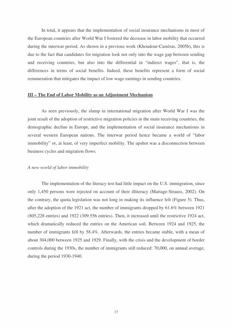
The implementation of the literacy test had little impact on the U.S. immigration, since
only 1,450 persons were rejected on account of their illiteracy (Mariage-Strauss, 2002). On
the contrary, the quota legislation was not long in making its influence felt (Figure 5). Thus,
after the adoption of the 1921 act, the number of immigrants dropped by 61.6% between 1921
(805,228 entries) and 1922 (309.556 entries). Then, it increased until the restrictive 1924 act,
which dramatically reduced the entries on the American soil. Between 1924 and 1925, the
number of immigrants fell by 58.4%. Afterwards, the entries became stable, with a mean of
about 304,000 between 1925 and 1929. Finally, with the crisis and the development of border
controls during the 1930s, the number of immigrants still reduced: 70,000, on annual average,
during the period 1930-1940.
18
Figure 5
Immigration to the United States: 1918-1940
111141
430
805
310
523
707
294 304335
307280
242
97
36 23 29 35 36 50 68 83 71
0
100
200
300
400
500
600
700
800
90019
18
1919
1920
1921
1922
1923
1924
1925
1926
1927
1928
1929
1930
1931
1932
1933
1934
1935
1936
1937
1938
1939
1940
Thou
sand
s of
imm
igra
nts
Source: Mitchell (2003).
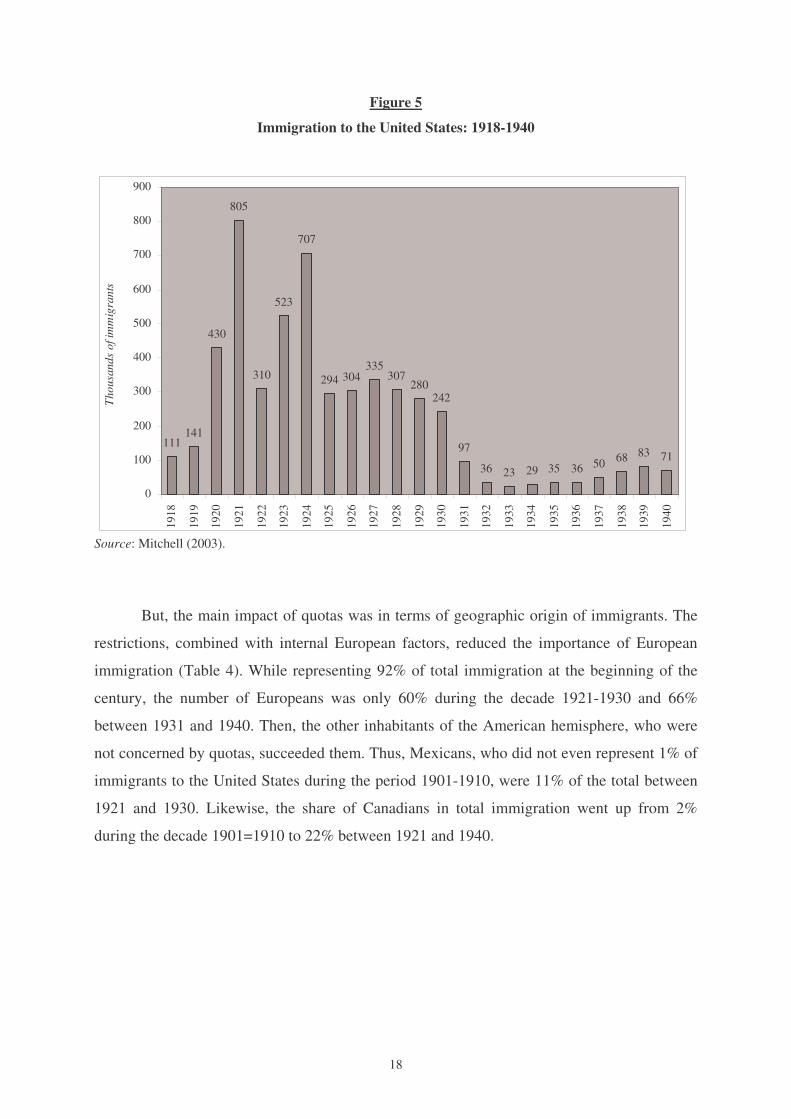
But, the main impact of quotas was in terms of geographic origin of immigrants. The
restrictions, combined with internal European factors, reduced the importance of European
immigration (Table 4). While representing 92% of total immigration at the beginning of the
century, the number of Europeans was only 60% during the decade 1921-1930 and 66%
between 1931 and 1940. Then, the other inhabitants of the American hemisphere, who were
not concerned by quotas, succeeded them. Thus, Mexicans, who did not even represent 1% of
immigrants to the United States during the period 1901-1910, were 11% of the total between
1921 and 1930. Likewise, the share of Canadians in total immigration went up from 2%
during the decade 1901=1910 to 22% between 1921 and 1940.
19
Table 4
Number of immigrants to the United States by decade
Origin region “Old Europe” “New Europe” Total Europe All countries
1901-1910 1.910.035
22% 24%
6.146.005 70% 76%
8.056.040 92%
100%
8.795.386 100%
1911-1920 997.438
15% 23%
3.324.449 60% 77%
4.321.887 75%
100%
5.735.811 100%
1921-1930 1.283.296
31% 52%
1.179.898 29% 48%
2.463.194 60%
100%
4.107.209 100%
1931-1940 197.964
38% 57%
149.602 28% 43%
347.566 66%
100%
528.431 100%
Note: “Old Europe” refers to traditional immigration countries, that is, western and northern European countries: Belgium, Denmark, France, Germany, Ireland, the Netherlands, Norway, Sweden, Switzerland and the United Kingdom. “New Europe” includes recent immigration countries, i.e. eastern and southern Europe: Austria, Czechoslovakia, Greece, Hungary, Italy, Poland, Portugal, Romania, Russia, Spain, Yugoslavia, etc. Source: U.S. Immigration and Naturalization Service (2003).
In other respects, quota laws resulted in a reallocation of migration in favor of “old
Europe” citizens. These, who represented less than a quarter of European immigration during
the first two decades of the twentieth century, became the majority again in the 1920s and
1930s. Not really because of a significant increase in the number of immigrants originating
from western and northern Europe, but rather due to the fall in immigration from eastern and
southern Europeans. Thus, whereas the number of immigrants proceeding from the “old
Europe” increased by 29% between the decades 1911-1920 and 1921-1930, the number of
“new Europeans” dropped by 65%; meanwhile, total immigration fall by 28%. By the same
token, the 1930s were marked by a drastic reduction of the immigration to the United States,
but eastern and southern Europeans were especially affected, with a drop by 87% between the
decade 1921-1930 and the following one. They then represented 43% of immigrant cohorts
coming from Europe and only 28% of total immigration.
In total, border control measures implemented by American authorities achieved their
twofold purpose: first of all, to reduce total immigration; second of all, to specifically affect
southern and eastern European countries. “Discrimination exerts its effects. Countries such as
20
Great Britain, Ireland, Germany, which benefit from a significant quota, do not fulfill it. In
Greece, in Italy, in eastern Europe, lines grow longer in front of American consulates in
order to obtain the precious visa. When the Nazi persecution pounces on the Jews, the State
Department declares itself bound by the quota legislation and sparingly allowed those
threatened by the worst extermination to enter.” (Kaspi, 1986: 19).
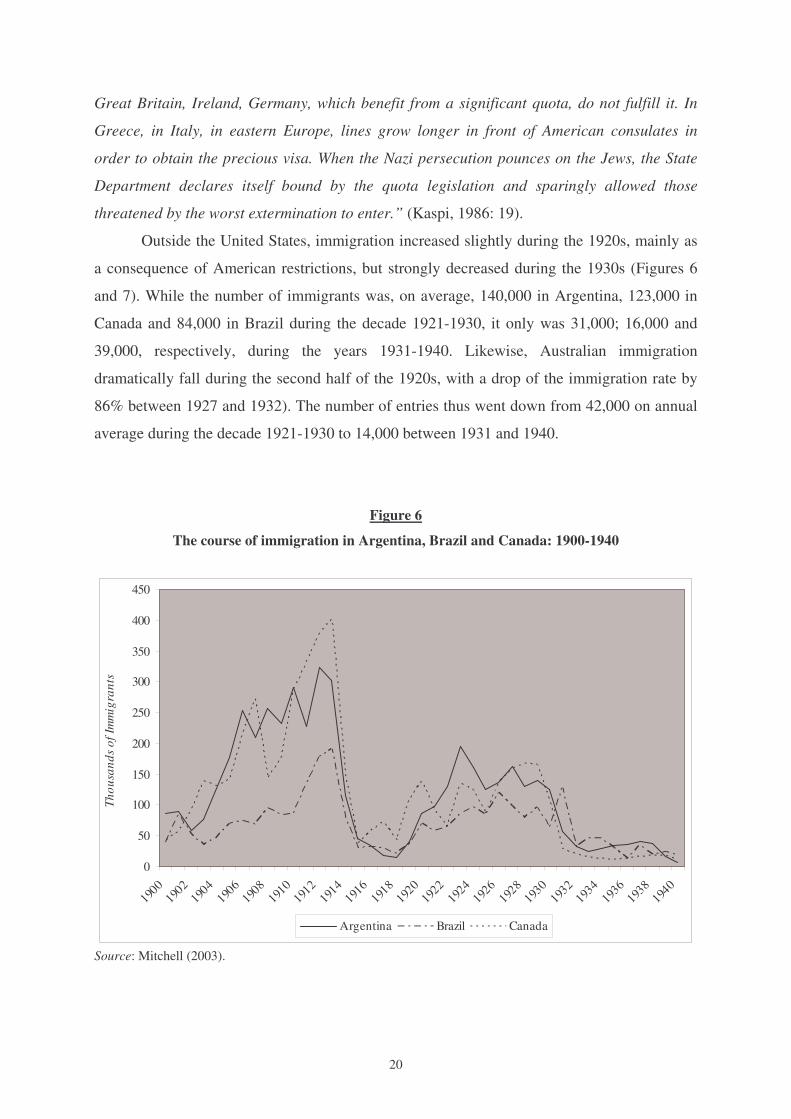
Outside the United States, immigration increased slightly during the 1920s, mainly as
a consequence of American restrictions, but strongly decreased during the 1930s (Figures 6
and 7). While the number of immigrants was, on average, 140,000 in Argentina, 123,000 in
Canada and 84,000 in Brazil during the decade 1921-1930, it only was 31,000; 16,000 and
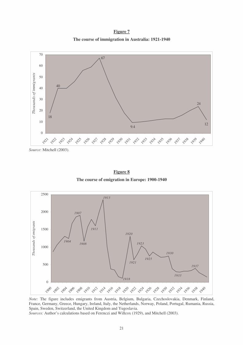
39,000, respectively, during the years 1931-1940. Likewise, Australian immigration
dramatically fall during the second half of the 1920s, with a drop of the immigration rate by
86% between 1927 and 1932). The number of entries thus went down from 42,000 on annual
average during the decade 1921-1930 to 14,000 between 1931 and 1940.
Figure 6
The course of immigration in Argentina, Brazil and Canada: 1900-1940
0
50
100
150
200
250
300
350
400
450
1900
1902
1904
1906
1908
1910
1912
1914
1916
1918
1920
1922
1924
1926
1928
1930
1932
1934
1936
1938
1940
Thou
sand
s of
Imm
igra
nts
Argentina Brazil Canada
Source: Mitchell (2003).
21
Figure 7
The course of immigration in Australia: 1921-1940
24
12
18
40
67
9.4
0
10
20
30
40
50
60
70
1921
1922
1923
1924
1925
1926
1927
1928
1929
1930
1931
1932
1933
1934
1935
1936
1937
1938
1939
1940
Thou
sand
s of
imm
igra
nts
Source: Mitchell (2003).
Figure 8
The course of emigration in Europe: 1900-1940
1937
1930
1925
1923
1921
1920
1918
1913
1911
1908
1907
1904
1933
0
500
1000
1500
2000
2500
1900
1902
1904
1906
1908
1910
1912
1914
1916
1918
1920
1922
1924
1926
1928
1930
1932
1934
1936
1938
1940
Thou
sand
s of
em
igra
nts
Note: The figure includes emigrants from Austria, Belgium, Bulgaria, Czechoslovakia, Denmark, Finland, France, Germany, Greece, Hungary, Ireland, Italy, the Netherlands, Norway, Poland, Portugal, Rumania, Russia, Spain, Sweden, Switzerland, the United Kingdom and Yugoslavia. Sources: Author’s calculations based on Ferenczi and Willcox (1929), and Mitchell (2003).
22
The change in migration patterns was also remarkable on the emigration countries
side. While the average annual number of European emigrants was around 1.6 millions
between 1901 and 1913, there were 857,000 average annual departures in the 1920s, and
hardly 356,000 in the 1930s (see figure 8). At the national level, the decline was very
impressive too. Indeed, with the notable exception of Denmark, which recorded a slight
increase in emigration rate during the 1930s, emigration dropped in all European countries
after World War I. Thus, Table 5 shows that between the periods 1900-1913 and 1930-1939
the emigration rate decreased by more than 40% in most of the European countries.
Scandinavian and Central European countries were the first affected by this phenomenon
since the emigration rate in these regions was below 0.5‰ after 1930. In that sense, the
implementation of quotas in the United States particularly hit countries like Austria and
Hungary.
Table 5
The course of emigration rates in Europe: 1900-1939
(a)
1900-1913
(b)
1920-1929
(c)
1930-1939
(d) % change
(b)/(a)
(e) % change
(c)/(b)
(f) % change
(c)/(a) Austria 17.61 0.97 0.37 -94.5 -61.6 -97.9
Hungary 6.47 0.65 0.20 -90.0 -69.4 -96.9
Norway 7.17 3.23 0.31 -54.9 -90.5 -95.7
Finland 5.33 1.83 0.34 -65.6 -81.4 -93.6
Sweden 4.52 2.21 0.46 -51.0 -79.3 -89.9
United Kingdom 7.16 3.85 0.80 -46.2 -79.3 -88.8
Ireland 7.82 7.39 0.91 -5.5 -87.7 -88.4
Spain 7.71 4.05 0.95 -47.5 -76.4 -87.6
Italy 17.05 7.58 2.13 -55.5 -71.9 -87.5
France 0.18 0.14 0.03 -22.2 -78.6 -83.3
Portugal 7.09 5.88 1.66 -17.0 -71.8 -76.6
Switzerland 1.40 1.49 0.47 +6.0 -68.6 -66.7
Belgium 4.21 4.34 2.18 +2.9 -49.6 -48.2
Germany 0.44 0.84 0.26 +88.6 -68.3 -40.3
Netherlands 5.64 6.19 5.50 +9.8 -11.1 -2.4
Denmark 2.64 2.31 2.68 -12.5 +15.7 +1.2 Note: Columns a, b and c represent the average annual emigration rate. Columns d, e and f show the total change in percent, respectively, between the periods 1920-1929 and 1900-1913, between the periods 1930-1939 and 1920-1929, and between the periods 1930-1939 and 1900-1913. Source: Author’s calculations based on Ferenczi and Willcox (1929), and Mitchell (2003).
23
The end of the relationship between labor mobility and business cycles
The combined action of restrictive migration policies in the New World and social
reforms in Europe had the effect of reducing international migration flows. As a result, labor
mobility stopped playing the role of adjustment mechanism that it had before World War I.
Thus, in the United States, while the correlation coefficient between the GDP growth rate and
the immigration growth rate was 0.7 for the period 1891-1913 (the growth of the GDP
entailed a rise in immigration), it was only -0.3 for 1920-1940. The correlation coefficient
between unemployment and immigration growth rates, as for it, was -0.6 for the first period
(an increase in the unemployment rate brought about a fall in the immigration rate), and 0.2
for the second one.
The consequences of migration barriers were also felt by European countries,
especially by those that tried to maintain both the stability and the convertibility of their
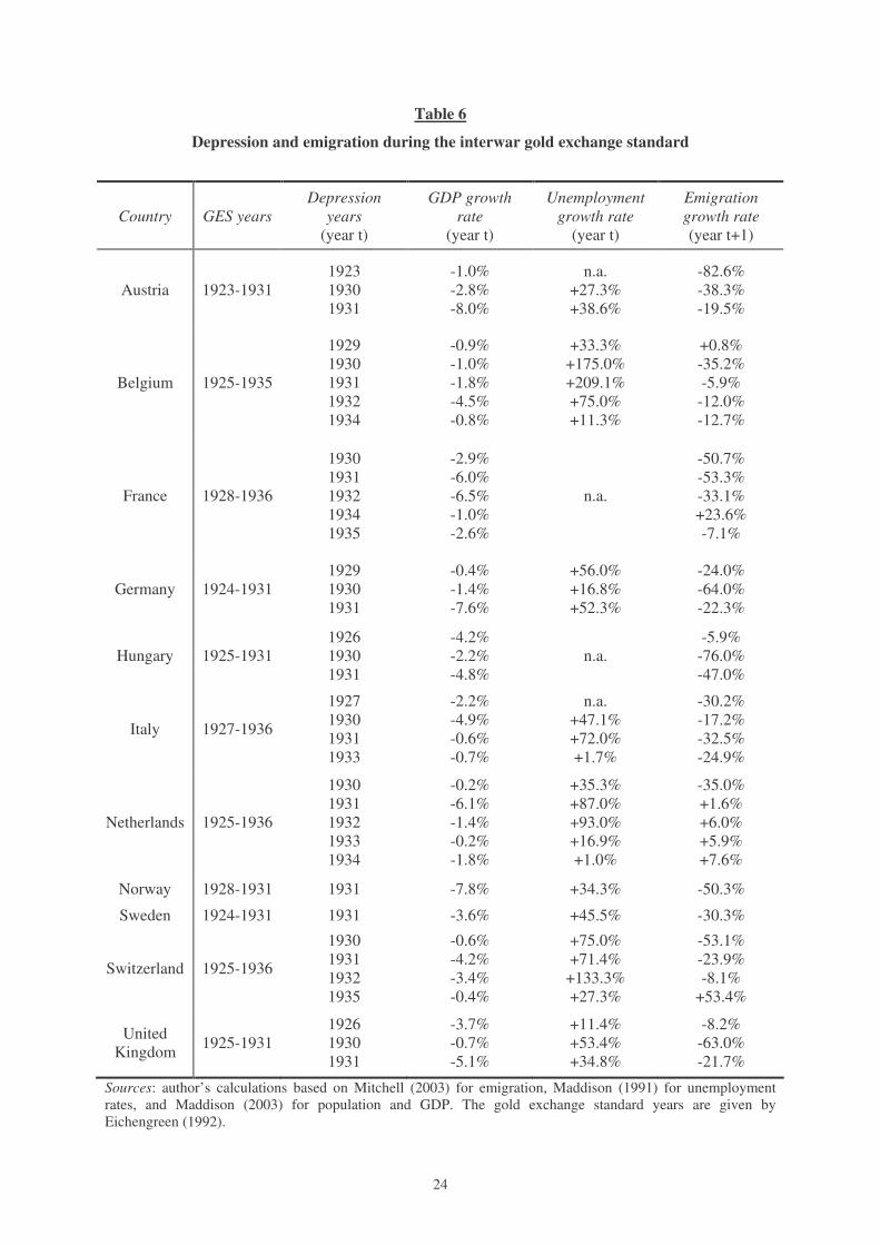
currency, especially the “gold bloc” countries. Table 6 shows that when the members of the
interwar gold exchange standard were affected by an economic crisis, the emigration rate did
not follow the expected pattern. Indeed, instead of increasing, as it did during the gold
standard period, emigration in Europe tended to fall after a depression. Thus, a drop in the
GDP was followed by a decrease in the emigration rate in 30 out of 37 cases (81% of the
cases), while an increase in the unemployment rate was accompanied by a fall in the
emigration rate in 21 out of 27 cases (78% of the cases).
24
Table 6
Depression and emigration during the interwar gold exchange standard
Country GES years Depression
years (year t)
GDP growth rate
(year t)
Unemployment growth rate
(year t)
Emigration growth rate (year t+1)
Austria 1923-1931 1923 1930 1931
-1.0% -2.8% -8.0%
n.a. +27.3% +38.6%
-82.6% -38.3% -19.5%
Belgium 1925-1935
1929 1930 1931 1932 1934
-0.9% -1.0% -1.8% -4.5% -0.8%
+33.3% +175.0% +209.1% +75.0% +11.3%
+0.8% -35.2% -5.9%
-12.0% -12.7%
France 1928-1936
1930 1931 1932 1934 1935
-2.9% -6.0% -6.5% -1.0% -2.6%
n.a.
-50.7% -53.3% -33.1% +23.6% -7.1%
Germany 1924-1931 1929 1930 1931
-0.4% -1.4% -7.6%
+56.0% +16.8% +52.3%
-24.0% -64.0% -22.3%
Hungary 1925-1931 1926 1930 1931
-4.2% -2.2% -4.8%
n.a. -5.9%
-76.0% -47.0%
Italy 1927-1936
1927 1930 1931 1933
-2.2% -4.9% -0.6% -0.7%
n.a. +47.1% +72.0% +1.7%
-30.2% -17.2% -32.5% -24.9%
Netherlands 1925-1936
1930 1931 1932 1933 1934
-0.2% -6.1% -1.4% -0.2% -1.8%
+35.3% +87.0% +93.0% +16.9% +1.0%
-35.0% +1.6% +6.0% +5.9% +7.6%
Norway 1928-1931 1931 -7.8% +34.3% -50.3%
Sweden 1924-1931 1931 -3.6% +45.5% -30.3%
Switzerland 1925-1936
1930 1931 1932 1935
-0.6% -4.2% -3.4% -0.4%
+75.0% +71.4%
+133.3% +27.3%
-53.1% -23.9% -8.1%
+53.4%
United Kingdom 1925-1931
1926 1930 1931
-3.7% -0.7% -5.1%
+11.4% +53.4% +34.8%
-8.2% -63.0% -21.7%
Sources: author’s calculations based on Mitchell (2003) for emigration, Maddison (1991) for unemployment rates, and Maddison (2003) for population and GDP. The gold exchange standard years are given by Eichengreen (1992).
25
Eventually, this is a confirmation of the fact that labor mobility can play a role of
safety valve in fixed exchange rate regimes only if there are enough employment
opportunities in at least one country. It is because the New World in general and the United
States in particular were able – and eager – to absorb a large amount of labor before World
War I that European workers could settle abroad when domestic conditions worsened. But, it
was not until 1938 that the American GDP attained again its 1929 level; and the
unemployment rate was 18.3%, on annual average, between 1930 and 1939, which clearly
meant that foreign workers were not welcome in the United States, as confirmed by a
discourse made by Franklin Roosevelt during the 1932 presidential campaign: “Our last
frontier has long since been reached, and there is practically no more free land. More than
half of our people do not live on the farms or on lands and cannot derive a living by
cultivating their own property. There is no safety valve in the form of a Western prairie to
which those thrown out of work by the Eastern economic machines can go for a new start. We
are not able to invite the immigration from Europe to share our endless plenty. We are now
providing a drab living for our own people.” (Roosevelt, 1932).
IV - On the Impact of Labor Immobility on the Fall of the Interwar Gold Exchange
Standard
It is likely that the success of the classical gold standard before World War I was
indirectly the result of the labor shortage in New World countries. Their development
potential was constrained by the lack of labor force and they generally had very active
immigration policies in order to fill the fields and the factories with foreign manpower. To the
contrary, the nineteenth century population explosion in Europe brought about a huge labor
surplus that could only be solved thanks to the departure of a large number of workers for the
far shores of the Americas or Oceania. This migration process was made easier by the
existence of significant wage differentials between sending and receiving countries. Besides,
labor movements were strongly sensitive to business cycles and changes in employment
conditions: a rise in the foreign economic activity and/or a decrease in the domestic economy
entailed a surge in migration, whereas a recession in the receiving countries and/or an
expansion at home resulted in fewer movements. Then, the countries that belonged to the gold
standard could rest on labor mobility to mitigate the effects of exchange rate stability
(Khoudour-Castéras, 2005a). But, after World War I, when labor turned out to be surplus in
26
the main host countries, potential migrants had to stay at home, with the consequence that the
adjustment became more difficult. The gold exchange standard could not withstand this new
situation.
Labor mobility and the adjustment problem of the gold exchange standard
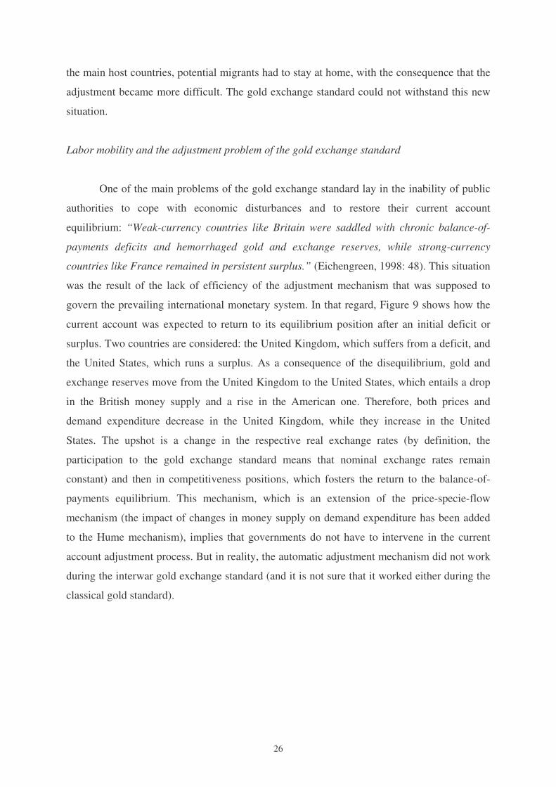
One of the main problems of the gold exchange standard lay in the inability of public
authorities to cope with economic disturbances and to restore their current account
equilibrium: “Weak-currency countries like Britain were saddled with chronic balance-of-
payments deficits and hemorrhaged gold and exchange reserves, while strong-currency
countries like France remained in persistent surplus.” (Eichengreen, 1998: 48). This situation
was the result of the lack of efficiency of the adjustment mechanism that was supposed to
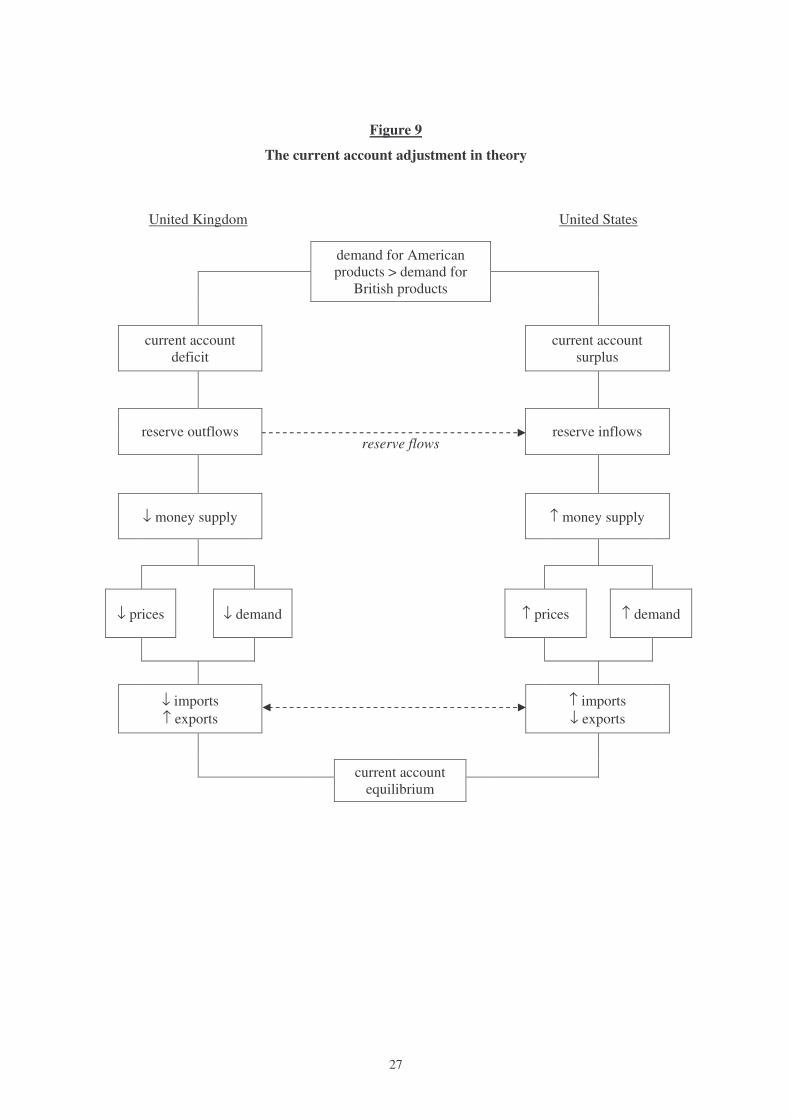
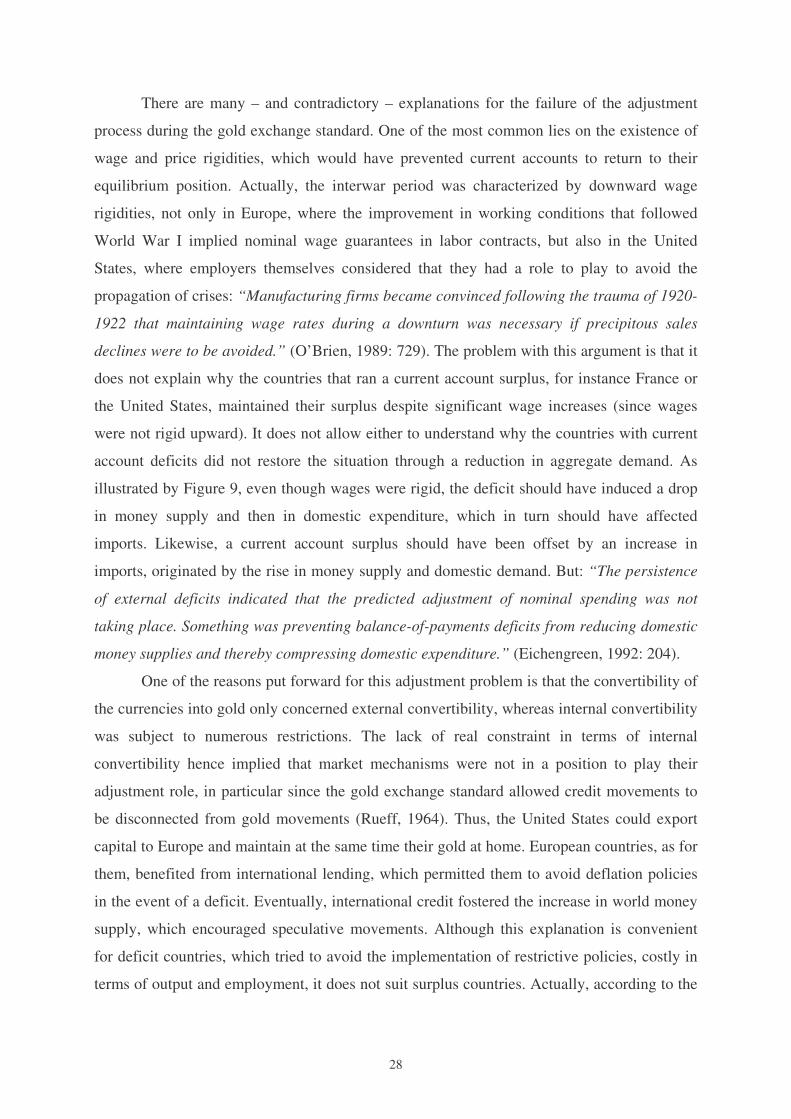
govern the prevailing international monetary system. In that regard, Figure 9 shows how the
current account was expected to return to its equilibrium position after an initial deficit or
surplus. Two countries are considered: the United Kingdom, which suffers from a deficit, and
the United States, which runs a surplus. As a consequence of the disequilibrium, gold and
exchange reserves move from the United Kingdom to the United States, which entails a drop
in the British money supply and a rise in the American one. Therefore, both prices and
demand expenditure decrease in the United Kingdom, while they increase in the United
States. The upshot is a change in the respective real exchange rates (by definition, the
participation to the gold exchange standard means that nominal exchange rates remain
constant) and then in competitiveness positions, which fosters the return to the balance-of-
payments equilibrium. This mechanism, which is an extension of the price-specie-flow
mechanism (the impact of changes in money supply on demand expenditure has been added
to the Hume mechanism), implies that governments do not have to intervene in the current
account adjustment process. But in reality, the automatic adjustment mechanism did not work
during the interwar gold exchange standard (and it is not sure that it worked either during the
classical gold standard).
27
Figure 9
The current account adjustment in theory
United Kingdom United States
demand for American products > demand for
British products
current account deficit current account
surplus
reserve outflows
reserve flows reserve inflows
↓ money supply ↑ money supply
↓ prices ↓ demand ↑ prices ↑ demand
↓ imports ↑ exports
↑ imports
↓ exports
current account
equilibrium
28
There are many – and contradictory – explanations for the failure of the adjustment
process during the gold exchange standard. One of the most common lies on the existence of
wage and price rigidities, which would have prevented current accounts to return to their
equilibrium position. Actually, the interwar period was characterized by downward wage
rigidities, not only in Europe, where the improvement in working conditions that followed
World War I implied nominal wage guarantees in labor contracts, but also in the United
States, where employers themselves considered that they had a role to play to avoid the
propagation of crises: “Manufacturing firms became convinced following the trauma of 1920-
1922 that maintaining wage rates during a downturn was necessary if precipitous sales
declines were to be avoided.” (O’Brien, 1989: 729). The problem with this argument is that it
does not explain why the countries that ran a current account surplus, for instance France or
the United States, maintained their surplus despite significant wage increases (since wages
were not rigid upward). It does not allow either to understand why the countries with current
account deficits did not restore the situation through a reduction in aggregate demand. As
illustrated by Figure 9, even though wages were rigid, the deficit should have induced a drop
in money supply and then in domestic expenditure, which in turn should have affected
imports. Likewise, a current account surplus should have been offset by an increase in
imports, originated by the rise in money supply and domestic demand. But: “The persistence
of external deficits indicated that the predicted adjustment of nominal spending was not
taking place. Something was preventing balance-of-payments deficits from reducing domestic
money supplies and thereby compressing domestic expenditure.” (Eichengreen, 1992: 204).
One of the reasons put forward for this adjustment problem is that the convertibility of
the currencies into gold only concerned external convertibility, whereas internal convertibility
was subject to numerous restrictions. The lack of real constraint in terms of internal
convertibility hence implied that market mechanisms were not in a position to play their
adjustment role, in particular since the gold exchange standard allowed credit movements to
be disconnected from gold movements (Rueff, 1964). Thus, the United States could export
capital to Europe and maintain at the same time their gold at home. European countries, as for
them, benefited from international lending, which permitted them to avoid deflation policies
in the event of a deficit. Eventually, international credit fostered the increase in world money
supply, which encouraged speculative movements. Although this explanation is convenient
for deficit countries, which tried to avoid the implementation of restrictive policies, costly in
terms of output and employment, it does not suit surplus countries. Actually, according to the
29
lack-of-constraint logic, the U.S. money supply should have increased since capital outflows
were not accompanied by gold outflows.
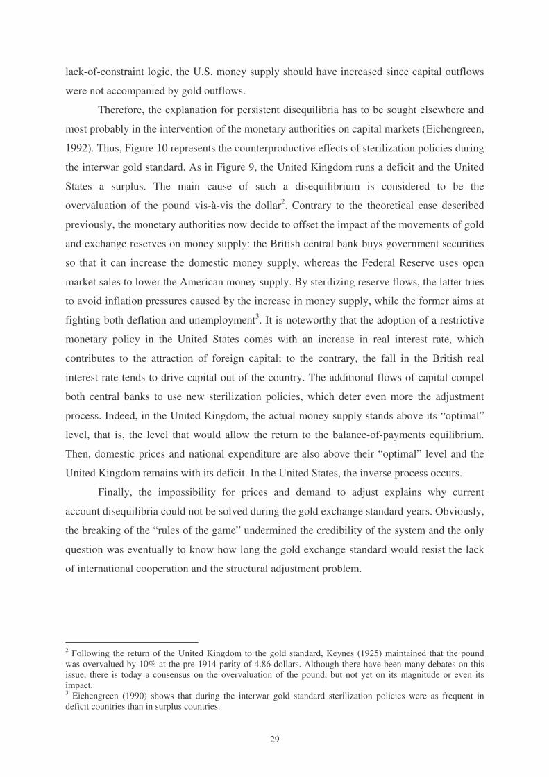
Therefore, the explanation for persistent disequilibria has to be sought elsewhere and
most probably in the intervention of the monetary authorities on capital markets (Eichengreen,
1992). Thus, Figure 10 represents the counterproductive effects of sterilization policies during
the interwar gold standard. As in Figure 9, the United Kingdom runs a deficit and the United
States a surplus. The main cause of such a disequilibrium is considered to be the
overvaluation of the pound vis-à-vis the dollar2. Contrary to the theoretical case described
previously, the monetary authorities now decide to offset the impact of the movements of gold
and exchange reserves on money supply: the British central bank buys government securities
so that it can increase the domestic money supply, whereas the Federal Reserve uses open
market sales to lower the American money supply. By sterilizing reserve flows, the latter tries
to avoid inflation pressures caused by the increase in money supply, while the former aims at
fighting both deflation and unemployment3. It is noteworthy that the adoption of a restrictive
monetary policy in the United States comes with an increase in real interest rate, which
contributes to the attraction of foreign capital; to the contrary, the fall in the British real
interest rate tends to drive capital out of the country. The additional flows of capital compel
both central banks to use new sterilization policies, which deter even more the adjustment
process. Indeed, in the United Kingdom, the actual money supply stands above its “optimal”
level, that is, the level that would allow the return to the balance-of-payments equilibrium.
Then, domestic prices and national expenditure are also above their “optimal” level and the
United Kingdom remains with its deficit. In the United States, the inverse process occurs.
Finally, the impossibility for prices and demand to adjust explains why current
account disequilibria could not be solved during the gold exchange standard years. Obviously,
the breaking of the “rules of the game” undermined the credibility of the system and the only
question was eventually to know how long the gold exchange standard would resist the lack
of international cooperation and the structural adjustment problem.
2 Following the return of the United Kingdom to the gold standard, Keynes (1925) maintained that the pound was overvalued by 10% at the pre-1914 parity of 4.86 dollars. Although there have been many debates on this issue, there is today a consensus on the overvaluation of the pound, but not yet on its magnitude or even its impact. 3 Eichengreen (1990) shows that during the interwar gold standard sterilization policies were as frequent in deficit countries than in surplus countries.
30
Figure 10
The gold exchange standard in practice
United Kingdom United States
overvaluation of the pound/dollar
demand for American products > demand for
British products
current account deficit current account surplus
reserve outflows
reserve flows reserve inflows
capital flows
capital
outflows
capital inflows
expansive monetary
policy sterilization
policies
restrictive monetary
policy
↓ real interest
rate ↑ real interest
rate
actual money supply > “optimal” money supply actual money supply <
“optimal” money supply
actual prices >
equilibrium prices
actual demand >
equilibrium demand
actual prices <
equilibrium prices
actual demand <
equilibrium demand
deficit
persistent
disequilibria surplus
31
In total, among the many explanations for the adjustment problem of the gold
exchange standard, the most pertinent seems to be the frequent use of sterilization policies by
the interwar monetary authorities. Yet, it is also conceivable that the lack of labor mobility
during that period added to the balance-of-payments problem. As a matter of fact, the reason
why deficit countries chose to implement sterilization policies, that is, expansive monetary
policies, was the recessive impact of the automatic adjustment mechanism. The return to the
equilibrium position indeed lay on the fall in domestic prices. But the fact that wages were
rigid downwards slowed down the adjustment process and brought about an increase in
unemployment, worsened by the fall in national spending that followed the current account
deficit. The countries that enjoyed surpluses, as for them, aimed at reducing inflation
pressures that came with the increase in money supply caused by the current account surplus.
If migration movements would have been free, as they were before World War I, it is likely
that the increase in emigration would have reduced the need to use sterilization policies.
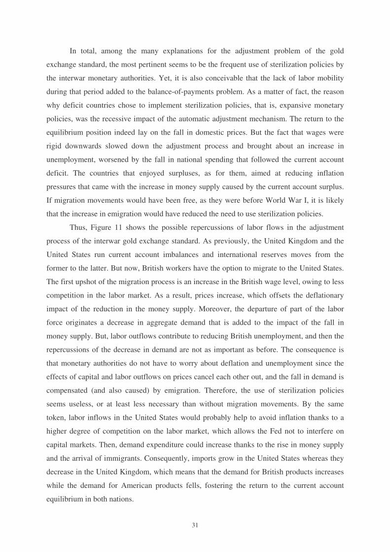
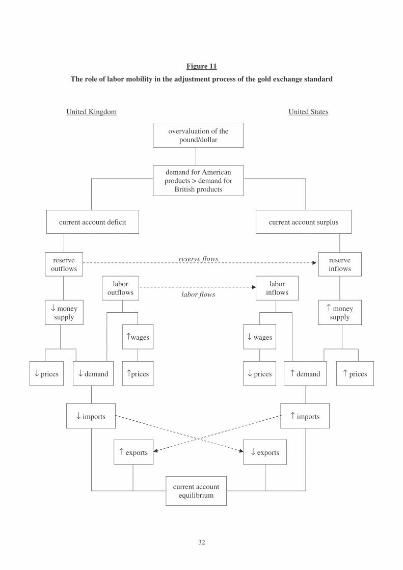
Thus, Figure 11 shows the possible repercussions of labor flows in the adjustment
process of the interwar gold exchange standard. As previously, the United Kingdom and the
United States run current account imbalances and international reserves moves from the
former to the latter. But now, British workers have the option to migrate to the United States.
The first upshot of the migration process is an increase in the British wage level, owing to less
competition in the labor market. As a result, prices increase, which offsets the deflationary
impact of the reduction in the money supply. Moreover, the departure of part of the labor
force originates a decrease in aggregate demand that is added to the impact of the fall in
money supply. But, labor outflows contribute to reducing British unemployment, and then the
repercussions of the decrease in demand are not as important as before. The consequence is
that monetary authorities do not have to worry about deflation and unemployment since the
effects of capital and labor outflows on prices cancel each other out, and the fall in demand is
compensated (and also caused) by emigration. Therefore, the use of sterilization policies
seems useless, or at least less necessary than without migration movements. By the same
token, labor inflows in the United States would probably help to avoid inflation thanks to a
higher degree of competition on the labor market, which allows the Fed not to interfere on
capital markets. Then, demand expenditure could increase thanks to the rise in money supply
and the arrival of immigrants. Consequently, imports grow in the United States whereas they
decrease in the United Kingdom, which means that the demand for British products increases
while the demand for American products fells, fostering the return to the current account
equilibrium in both nations.
32
Figure 11
The role of labor mobility in the adjustment process of the gold exchange standard
The limits of capital as an alternative adjustment mechanism
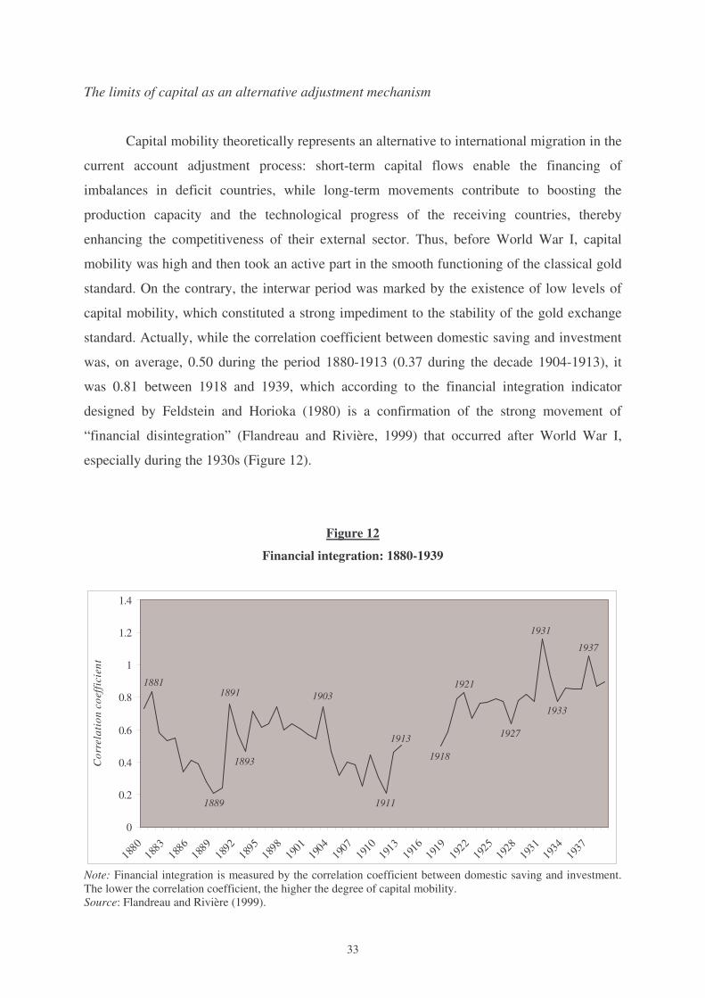
Capital mobility theoretically represents an alternative to international migration in the
current account adjustment process: short-term capital flows enable the financing of
imbalances in deficit countries, while long-term movements contribute to boosting the
production capacity and the technological progress of the receiving countries, thereby
enhancing the competitiveness of their external sector. Thus, before World War I, capital
mobility was high and then took an active part in the smooth functioning of the classical gold
standard. On the contrary, the interwar period was marked by the existence of low levels of
capital mobility, which constituted a strong impediment to the stability of the gold exchange
standard. Actually, while the correlation coefficient between domestic saving and investment
was, on average, 0.50 during the period 1880-1913 (0.37 during the decade 1904-1913), it
was 0.81 between 1918 and 1939, which according to the financial integration indicator
designed by Feldstein and Horioka (1980) is a confirmation of the strong movement of
“financial disintegration” (Flandreau and Rivière, 1999) that occurred after World War I,
especially during the 1930s (Figure 12).
Figure 12
Financial integration: 1880-1939
1933
1937
1931
1927
1921
1918
1913
1911
1903
1893
18911881
1889
0
0.2
0.4
0.6
0.8
1
1.2
1.4
1880
1883
1886
1889
1892
1895
1898
1901
1904
1907
1910
1913
1916
1919
1922
1925
1928
1931
1934
1937
Cor
rela
tion
coe
ffic
ient
Note: Financial integration is measured by the correlation coefficient between domestic saving and investment. The lower the correlation coefficient, the higher the degree of capital mobility. Source: Flandreau and Rivière (1999).
34
This breakdown in the financial integration process was fundamentally due to the
implementation of capital control policies after 1914. France and Germany, in particular,
tried, from the beginning of the conflict, to prevent gold withdrawals from their territory. This
is the reason why public authorities of both belligerent countries not only suspended the
convertibility of their currency into gold, but also, in the image of Great Britain, forbade gold
outflows. With the spread of the conflict and notably with the entry of the United States into
the war, capital controls (and not only on gold exports) increased: European countries aimed
to avoid the worsening of their currency depreciation, while the American government saw a
way to prevent that international lending finance the enemy’ war effort. At the end of the war,
heavily indebted countries were subject to the temptation of using seignoriage, which
produced speculative movements that the European governments tried to stop by
strengthening the controls.
The stabilization of most of the European economies a few years after the end of the
war and the return of the main currencies in the gold standard system in the middle of the
1920s furthered the progressive elimination of capital controls and then the recovery of
financial flows on an international scale (Obstfeld et Taylor, 1998). But, the American stock
exchange crash in 1929 had international repercussions that entailed the implementation of
new barriers to capital mobility: “The world economy went from globalized to almost autarkic
in the space of a few decades. Capital flows were minimal, international investment was
regarded with suspicion, and international prices and interest rates fell completely out of
synchronization. Global capital (along with finance in general) was demonized, and seen as a
principal cause of the world depression of the 1930s.” (Obstfeld and Taylor, 2003: 125).
Actually, the liberalization of capital flows itself originated the rapid transmission of the crisis
worldwide: American authorities reacted to the perturbations that affected Wall Street by
increasing their interest rates, which forced other countries, concerned about maintaining the
stability of their currency, to rise their own interest rates in order to avoid massive capital
outflows.
But, faced with the extent of speculative movements on both sides of the Atlantic and
after the international exchange crisis that followed the collapse of the Austrian Credit-Anstalt
in 1931, capital controls were established in most of the occidental countries and first of all in
Germany. The international conference held in London in July 1931 in order to prevent a new
depreciation of the mark had indeed formed the “Standstill Committee”, whose mission
consisted in studying the feasibility of a project aiming at immobilizing capitals in Germany:
“The decision to set up the Standstill Committee was to have unforeseen, far-reaching
35
consequences. It was to represent a definite turning point in the development of Western
civilization, which so far had been based on respect for contracts and monetary freedom; and
it would be possible to follow an internal inflationary policy without depreciating the
currency. In fine, it was the first step toward the institution of exchange control.”(Rueff,
1964: 11-12).
These measures then spread because the governments at the time did not consider
other riposte to capital flight than financial movement controls: “As in the past, applied
controls consist in defending or stabilizing exchange rate quotation, in having an influence on
foreign loans, etc. But, control policies also aim to isolate the domestic economy in order to
be able to implement recovery measures. […] National policies aiming at steering investment
flows by sectors therefore come with controls that permit to keep significant interest
differentials. Thus, governments can apply autonomous objectives. This is the ‘Big
Transformation’.” (Flandreau and Rivière, 1999: 25).
Resurgence of protectionism and rise in unemployment
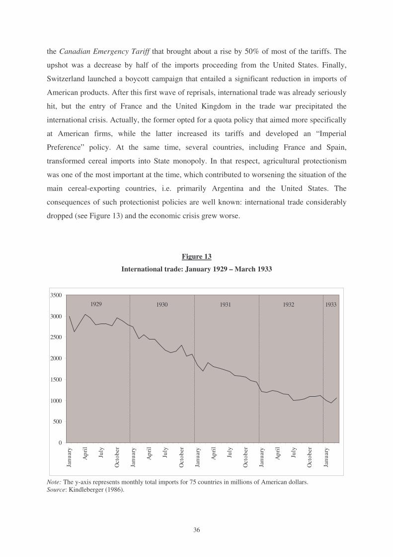
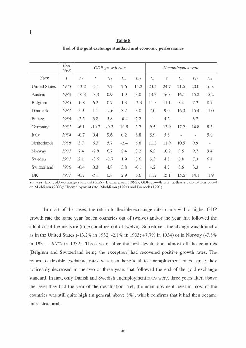
In view of the impossibility for public authorities to cope with economic disturbances
and current account imbalances, most of the countries decided to compensate the lack of labor
and capital mobility by resorting to trade protectionism. Against this backdrop, the signature
of the Smoot-Hawley Act by President Hoover, on the 17th of June of 1930 constituted the
starting point of the resurgence of protectionism on a world scale. Actually, whereas
American tariffs represented, on average, 31.3% of total imports during the period 1920-1925
and 40.3% in 1926-1930, they came to 55.3% during the years 1931-1933 (59.1% in 1932).
Such a rise ran counter to the conclusions of the international conference held in Geneva on
May 1927, in the course of which participating countries committed themselves to a “tariff
peace” (Bairoch, 1997). American trade partners felt betrayed and decided, as a reprisal, to
increase their own tariffs and/or to implement quotas on some American products (Jones,
1934).
Spain represents one of the most significant examples of the international reaction to
the Smoot-Hawley tariff, since it adopted the Wais tariff on July 22, that is, barely one month
after the American tariff. Car imports were primarily targeted: 473 American cars were
imported in 1932, as against 7,415 in 1920, which corresponds to a drop by 94%. In the same
way, Italy intended to protect the Fiat company by adopting a tariff on American cars, whose
price hence increased by about 135%. Canada, as for it, implemented on September 17, 1930
36
the Canadian Emergency Tariff that brought about a rise by 50% of most of the tariffs. The
upshot was a decrease by half of the imports proceeding from the United States. Finally,
Switzerland launched a boycott campaign that entailed a significant reduction in imports of
American products. After this first wave of reprisals, international trade was already seriously
hit, but the entry of France and the United Kingdom in the trade war precipitated the
international crisis. Actually, the former opted for a quota policy that aimed more specifically
at American firms, while the latter increased its tariffs and developed an “Imperial
Preference” policy. At the same time, several countries, including France and Spain,
transformed cereal imports into State monopoly. In that respect, agricultural protectionism
was one of the most important at the time, which contributed to worsening the situation of the
main cereal-exporting countries, i.e. primarily Argentina and the United States. The
consequences of such protectionist policies are well known: international trade considerably
dropped (see Figure 13) and the economic crisis grew worse.
Figure 13
International trade: January 1929 – March 1933
1932 1933193119301929
0
500
1000
1500
2000
2500
3000
3500
Janu
ary
Apr
il
July
Oct
ober
Janu
ary
Apr
il
July
Oct
ober
Janu
ary
Apr
il
July
Oct
ober
Janu
ary
Apr
il
July
Oct
ober
Janu
ary
Note: The y-axis represents monthly total imports for 75 countries in millions of American dollars. Source: Kindleberger (1986).
37
At the same time that the international crisis and the protectionist policies developed,
unemployment raised in most of the western countries. Indeed, the development of border
controls and the slowdown in international movements meant that unemployed persons had to
stay in their home country, which furthered the excess labor supply. It is also likely that the
implementation of unemployment insurance mechanisms in some European countries during
the interwar period contributed to raising the unemployment rate (see Section II), as in
England where the amount of unemployed persons was permanently above one million
between 1919 and 1940. This would explain non only the increase in cyclical unemployment
during economic crises, but also the development of structural unemployment from the
beginning of the 1920s (Table 7): “It is normal that the two countries where the 1920s were
negative on the economic level, that is, Germany and the United Kingdom, were
characterized by higher unemployment than before the war. But, what is significant is that the
phenomenon affected many countries. In fact, in addition to the case of the United States, a
‘low unemployment country’, only Belgium and Switzerland escaped from the appearance of
what it is possible to call structural unemployment.” (Bairoch, 1997: 48).
Table 7
The evolution of the average unemployment rate
1920-1929 1930-1938
Austria 5.91 12.8 Belgium 1.52 8.7 Denmark 8.1 10.9 Finland 1.6 4.1 France 1.73 3.54 Germany 3.9 8.8 Italy 1.75 4.8 Netherlands 2.3 8.7 Norway 5.62 8.1 Sweden 3.2 5.6 Switzerland 0.45 3.0 United Kingdom 7.5 11.5 United States 4.8 18.2 Notes: 1: 1924-1929; 2: 1921-1929; 3: 1921, 1926 and 1929; 4: 1931, 1936 and 1938; 5: only 1929. Source: Maddison (1991).
38
Of course, the 1929 crisis and the use of non-cooperative policies that came with it
contributed to strongly increase unemployment in affected countries. Thus, the American
unemployment rate was 8.7% in 1930, as against 3.6%, on average, during the period 1923-
1929. After the collapse of the economy at the beginning of the 1930s (-8.9% in 1930, -7.7%
in 1931, and -13.2% in 1932), it reached 23.6% in 1932 and 24.7% in 1933 (its historic
record). In the same way, many European countries registered unemployment rates above
10% during the years 1931-1933: 10.2% in Norway (1931), 11.9% in Belgium (1932), 15.3%
in the United Kingdom (1932), 16% in Denmark (1932), 16.3% in Austria (1933), 17.2% in
Germany (1932)… Australia (19.1% in 1932) and Canada (19.3% in 1933) were also affected
by the increase in world unemployment. As a result, contrary to the three or four decades that
preceded World War I, when mass migration permitted to absorb surplus labor, the Great
Depression did not offer many alternatives to job searchers, who came up against the anti-
migration legislations implemented all over the planet after 1918.
The fall of the gold exchange standard
Since the moment when the absorption capacity of the American labor market
vanished, labor mobility lost its regulation function and the stability of exchange rates became
a more difficult objective to reach. At the same time, wage flexibility and capital mobility,
which represents traditional substitutes to labor mobility in the adjustment process of fixed
exchange rate regimes, were strongly limited. To deal with the Great Depression, many
countries that tried to maintain the stability of their currency opted for protectionist policies,
but the only result was the worsening of the international crisis. Consequently, unemployment
rates dramatically increased and the defense of the gold exchange standard was economically,
socially and politically untenable. Obviously, the triggering of the crack of 1929 sped up the
decay process of the interwar international monetary system.
Thus, after the first attacks against Wall Street in October 1929 and the bursting of the
speculative bubble on American markets, European markets became affected and 1931,
notably, was a year of bank runs and massive capital withdrawals. Faced with speculation
movements, several Central Banks were induced to suspend the international convertibility of
their currency. The Bank of England, in particular, had to abandon the convertibility of the
pound on September 21, 1931, which caused ipso facto the depreciation of the British
currency. Afterwards, some twenty other countries opted for giving up the stability of the
exchange rate. When, in 1933, the new elected American President, Franklin Roosevelt,
39
decided to devaluate the dollar, the trade partners of the United States, including the “gold
bloc” countries, had no other option than to renounce to the prevailing monetary system. In
1937, the gold exchange standard did not exist anymore (Figure 14).
Figure 14
Number of countries in the gold exchange standard: 1921-1937
Sources: End gold exchange standard (GES): Eichengreen (1992); GDP growth rate: author’s calculations based on Maddison (2003); Unemployment rate: Maddison (1991) and Bairoch (1997).
In most of the cases, the return to flexible exchange rates came with a higher GDP
growth rate the same year (seven countries out of twelve) and/or the year that followed the
adoption of the measure (nine countries out of twelve). Sometimes, the change was dramatic
as in the United States (-13.2% in 1932, -2.1% in 1933; +7.7% in 1934) or in Norway (-7.8%
in 1931, +6.7% in 1932). Three years after the first devaluation, almost all the countries
(Belgium and Switzerland being the exception) had recovered positive growth rates. The
return to flexible exchange rates was also beneficial to unemployment rates, since they
noticeably decreased in the two or three years that followed the end of the gold exchange
standard. In fact, only Danish and Swedish unemployment rates were, three years after, above
the level they had the year of the devaluation. Yet, the unemployment level in most of the
countries was still quite high (in general, above 8%), which confirms that it had then became
more structural.
41
Even though, this improvement in economic performances is partly related to the
adoption of internal recovery policies, in particular the New Deal in the United States, the
return to exchange rate flexibility probably played a key role, since it fostered the return to the
equilibrium: “The problem was not that devaluation took place; it was that the practice was
not more widespread and that it did not prompt the adoption of even more expansionary
policies. Abandoning the gold standard allowed countries to regain their policy
independence. And by devoting some of that independence to policies of leaning against the
wind in currency markets, they were able to do so without allowing the foreign exchanges to
descend into chaos.” (Eichengreen, 1998: 90).
Conclusion
The brief experience of the gold exchange standard during the interwar period seems
to confirm the existence of a trade-off between labor mobility and exchange rate fluctuations
in the balance-of-payments adjustment process. The countries that opt for fixed exchange
rates need adjustment mechanisms to offset the loss of the exchange rate instrument. In the
absence of wage flexibility and capital mobility, international migration constitutes an
appropriate mechanism for solving both internal and external imbalances. In sending
countries, labor outflows contribute to reducing unemployment and also further the reduction
of current account deficits, since they imply a decrease in aggregate demand and then in
imports. In receiving countries, immigration enables to curb inflationary pressures at the same
time that it stimulates demand and thereby imports. The countries with flexible exchange
rates, as for them, can rely on the exchange rate flexibility to make the adjustment process
easier.
In that sense, the development of border controls after World War I, joint with the
adoption of social policies in many European nations, did not allow labor flows to play their
role of adjustment mechanism in the countries that chose to defend the stability of their
currency. Since during this period wage flexibility and capital mobility were also limited, the
economies that suffered the effects of the Great Depression had no other option, in a context
of economic war and increasing unemployment, than to abandon their fixed exchange rate
policy. In fact, trade protectionism was first used as an alternative to factor mobility, but the
outcome of such a strategy was counterproductive since it eventually resulted in a severe
contraction of the world trade and a dramatic rise in unemployment rates. On the contrary, the
42
return to the exchange rate flexibility fostered the return to growth and contributed to
lowering unemployment levels.
Does it mean that if labor had been freer to move the gold exchange standard would
have survived longer? It is rather difficult to answer this question since the crash of 1929
represents a chock that it is not easy to put aside in a counterfactual analysis. Yet it is possible
to provide some elements of response. First and foremost, it has been underscored in this
paper that many restrictive immigration policies were not adopted in a context of economic
recession, but rather of expansion. As a result, border controls produced a misallocation of
factors that probably slowed down the world economic development. Besides, the
underconsumption problem that partly led to the Great Depression of the 1930s could
probably have been mitigated by the increase in demand that traditionally comes with more
immigration. Moreover, labor flows, as seen in Section IV, would have saved the monetary
authorities from having to resort to counterproductive sterilization policies. Indeed, by
intervening on capital markets, central banks try to avoid inflation when there is a current
account surplus, and deflation in case of a deficit. Well, labor movements have precisely this
effect: emigration from deficit countries prevent wages and then prices from falling, since
there is less competition on the domestic labor market; conversely, labor inflows in surplus
countries contributes to reducing wage pressures, that is, inflation pressures. In addition, labor
mobility causes changes in aggregate demand that induce variations in imports and exports,
hence in current account positions. Finally, all the money that migrants send home also takes
part in the adjustment process, since remittances help to finance the current account deficit. In
that respect too, higher levels of international migration would have certainly made the
balance-of-payments adjustment easier and would have improved the functioning of the
interwar gold exchange standard.
43
References
Akerman, Sune (1976). “Theories and Methods of Migration Research.” From Sweden to America: A History of the Migration. Eds. Runblom, Harald and Hans Norman. Minneapolis: University of Minnesota Press. Bairoch, Paul (1997). Victoires et déboires: Histoire économique et sociale du monde du XVIe siècle à nos jours. Tome 3. Paris: Gallimard. Buchinagni, Norman and al. (1985). Continuous journey: A Social History of South Asians in Canada. Toronto: McClelland & Stewart. Castles, Stephen and Mark Miller (1998). The Age of Migration: International Population Movements in the Modern World. London: Macmillan Press. Collomp, Catherine (2003). “Labour Unions and the Nationalisation of Immigration Restriction in the United States, 1880-1924”. Migration Control in the North Atlantic World: The Evolution of State Practices in Europe and the United States from the French Revolution to the Inter-War Period. Eds. Fahrmeir, Andreas; Olivier Faron and Patrick Veil. New York, Oxford: Berghahn Books: 237-252. Daniels, Roger (1995). “The Growth of Restrictive Immigration Policies in the Colonies of Settlement”. The Cambridge Survey of World Migration. Ed. Cohen, Robin. Cambridge: University Press: 39-43. Dohse, Knuth (1981). Ausländische Arbeitnehmer und bürgerlicher Staat. Königstein: Hain. Eichengreen, Barry (1998). Globalizing Capital: A History of the International Monetary System. Princeton: Princeton University Press. Eichengreen, Barry (1992). Golden Fetters: The Gold Standard and the Great Depression, 1919-1939. New York, Oxford: Oxford University Press. Eichengreen, Barry (1990). “International Monetary Instability Between the Wars: Structural Flaws or Misguised Policies?” The Evolution of the International Monetary System: How Can Efficiency and Stability Be Attained? Eds. Suzuki, Yoshio; Junichi Miyake and Mitsuaki Okabe. Tokyo: University of Tokyo Press: 71-116. Feldstein, Martin and Charles Horioka (1980). “Domestic Saving and International Capital Flows”. The Economic Journal 90.358: 314-329. Flandreau, Marc and Chantal Rivière (1999). “La Grande ‘Retransformation’ ? Contrôles de capitaux et intégration financière internationale, 1880-1996.” Economie internationale 78: 11-58. Flora, Peter (1983). State, Economy, and Society in Western Europe, 1815-1975. Vol I: The Growth of Mass Democracies and Welfare States. Frankfurt: Campus Verlag.
44
Gemery, Henry (1994). “Immigrants and Emigrants: International migration and the US labor market in the Great Depression”. Migration and the International Labor Market : 1850-1939. Eds. Hatton, Timothy and Jeffrey Williamson. Londres, New York: Routledge: 175-199. Hanes, Christopher (1993). “The Development of Nominal Wage Rigidity in the Late 19th Century.” American Economic Review 83.4: 732-756. Hatton, Timothy and Jeffrey Williamson (1994). “What Drove the Mass Migrations from Europe in the Late Nineteenth Century?” Population and Development Review 20.4: 533-559. James, Harold (2001). The End of Globalization: Lessons from the Great Depression. Cambridge: Harvard University Press. Jones, Joseph (1934). Tariff Retaliation : Repercussions of the Smooth-Hawley Bill. Philadelphia: University of Pennsylvania Press. Jones, Maldwyn Allen (1992). American Immigration. Chicago: The University of Chicago Press. Kaspi, André (1986). “Qu’est-ce qu’un Américain?” L’Histoire 91: 10-25. Keynes, John Maynard (1925). The Economic Consequences of Mr. Churchill. London: Hogarth Press. Khoudour-Castéras, David (2005a). “International Adjustment under the Classical Gold Standard: The Migration Nexus.” Mimeo, University of California, Berkeley. Khoudour-Castéras, David (2005b). “The Impact of the Bismarck’s Social Legislation on German Emigration before World War I.” Mimeo, University of California, Berkeley. Khoudour-Castéras, David (2002). “Taux de change fixes et migrations internationales : L’étalon-or à l’aune de la théorie des zones monétaires optimales.” Revue de l’OFCE 82: 82-116. Kindleberger, Charles (1986). The World in Depression, 1929-1939. Berkeley, Los Angeles: University of California Press. Kirk, Dudley (1946). Europe’s Population in the Interwar Years. New York: Gordon and Breach. de Lepervanche, Marie (1975). “Australian immigrants, 1788-1940: Desired and Unwanted.” Eds. Wheelwright, Edward and Ken Buckley. Essays in the Political Economy of Australian Capitalism. Volume I. Sydney: Australia and New Zealand Book Company. Light, Ivan (1972). Ethnic Enterprise in America: Business and Welfare Among Chinese, Japanese, and Blacks. Berkeley: University of California Press. Maddison, Angus (1991). Dynamic Forces in Capitalist Development: A Long-Run Comparative View. Oxford, New York: Oxford University Press.
45
Maddison Angus (1995). L'économie mondiale 1820-1992 : analyse et statistiques. Paris: Center for development studies, OECD. Mariage-Strauss, Annie (2002). Les Etats-Unis face à l’immigration. Paris: Ellipses. Markus, Andrew (1979). Fear and Hatred: Purifying Australia and California, 1850-1901. Sydney: Hale & Iremonger. Mitchell, Brian (2003a). International Historical Statistics: Europe, 1750-2000. London: Macmillan Reference Ltd, 5th ed. Mitchell, Brian (2003b). International Historical Statistics: The Americas, 1750-2000. London: Macmillan Reference Ltd, 5th ed. Mitchell, Daniel (1985). “Wage Flexibility: Then and Now.” Industrial Relations 24.2: 266-79. Mundell, Robert (1961). “A Theory of Optimum Currency Areas.” American Economic Review 51.4: 657-665. Nurkse, Ragnar (1944). International Currency Experience. Geneva: League of Nations. O’Brien, Anthony Patrick (1989). “A Behavioral Explanation for Nominal Wage Rigidity during the Great Depression.” Quarterly Journal of Economics 104.4: 719-35. Obstfeld, Maurice and Alan Taylor (2003). “Globalization and Capital Markets.” Eds. Bordo, Michael; Alan Taylor and Jeffrey Williamson. Globalization in Historical Perspective. Chicago, London: The University of Chicago Press: 121-187. Obstfeld, Maurice and Alan Taylor (1998). “The Great Depression as a Watershed: International Capital Mobility over the Long Run.” Eds. Bordo, Michael; Claudia Goldin and Eugene White. The Defining Moment: The Great Depression and the American Economy in the Twentieth Century. Chicago, London: The University of Chicago Press: 353-402. O’Rourke, Kevin and Jeffrey Williamson (1999). Globalization and History. Cambridge, Massachussets and London, England: The MIT Press. Palyi, Melchior (1972). The Twilight of Gold, 1914-1936. Chicago: Henry Regnery Company. Roosevelt, Franklin (1932). Commonwealth Club Address. San Francisco, September 23: http://www.americanrhetoric.com/speeches/fdrcommonwealth.htm. Rueff, Jacques (1964). The Age of Inflation. Chicago: Gateway Editions. Henry Regnery Company. Timmer, Ashley and Jeffrey Williamson (1998). “Immigration Policy Prior to the Thirties: Labor Markets, Policy Interactions and Globalization Backlash.”
46
United States Department of Commerce (1925-1941). Statistical Abstract of the United States. Washington, D.C.: U.S. Government Printing Office. United States Immigration Commission (1911). Reports. 61st Congress, 3rd Session, Washington, D.C.: U.S. Government Printing Office. United States Immigration and Naturalization Service (2003). Statistical Yearbook of the Immigration and Naturalization Service, 2002. Washington, D.C.: U.S. Government Printing Office. Weil, Patrick (1991). La France et ses étrangers: l'aventure d'une politique de l'immigration de 1938 à nos jours. Paris: Calmann-Lévy. Williamson, Jeffrey (1996). “Globalization, Convergence and History”. Journal of Economic History 56.2: 277-306.