DISCUSSION PAPER SERIES Forschungsinstitut zur Zukunft der Arbeit Institute for the Study of Labor Labor Supply Elasticities in Europe and the US IZA DP No. 5820 June 2011 Olivier Bargain Kristian Orsini Andreas Peichl
Transcript
DI
SC
US
SI
ON
P
AP
ER
S
ER
IE
S
Forschungsinstitut zur Zukunft der ArbeitInstitute for the Study of Labor
Any opinions expressed here are those of the author(s) and not those of IZA. Research published in this series may include views on policy, but the institute itself takes no institutional policy positions. The Institute for the Study of Labor (IZA) in Bonn is a local and virtual international research center and a place of communication between science, politics and business. IZA is an independent nonprofit organization supported by Deutsche Post Foundation. The center is associated with the University of Bonn and offers a stimulating research environment through its international network, workshops and conferences, data service, project support, research visits and doctoral program. IZA engages in (i) original and internationally competitive research in all fields of labor economics, (ii) development of policy concepts, and (iii) dissemination of research results and concepts to the interested public. IZA Discussion Papers often represent preliminary work and are circulated to encourage discussion. Citation of such a paper should account for its provisional character. A revised version may be available directly from the author.
IZA Discussion Paper No. 5820 June 2011
ABSTRACT
Labor Supply Elasticities in Europe and the US* Despite numerous studies on labor supply, the size of elasticities is rarely comparable across countries. In this paper, we suggest the first large-scale international comparison of elasticities, while netting out possible differences due to methods, data selection and the period of investigation. We rely on comparable data for 17 European countries and the US, a common empirical approach and a complete simulation of tax-benefit policies affecting household budgets. We find that wage-elasticities are small and vary less across countries than previously thought, e.g., between .2 and .6 for married women. Results are robust to several modeling assumptions. We show that differences in tax-benefit systems or demographic compositions explain little of the cross-country variation, leaving room for other interpretations, notably in terms of heterogeneous work preferences. We derive important implications for research on optimal taxation. JEL Classification: C25, C52, H31, J22 Keywords: household labor supply, elasticity, taxation, Europe, US Corresponding author: Olivier Bargain UCD Newman Building Dublin 4 Ireland E-mail: [email protected]
* The authors are grateful to R. Blundell, M. Dolls, D. Hamermesh, D. Neumann, S. Siegloch, A. van Soest and participants to seminars/workshops at UCD, IZA, ISER, Leuven, ZEW. Research was partly conducted during Peichl’s visit to the ECASS and ISER and supported by the Access to Research Infrastructures action (EU IHP Program) and the Deutsche Forschungsgemeinschaft (PE1675). We are indebted to the EUROMOD consortium and to Daniel Feenberg and the NBER for granting us access to TAXSIM and for help with the simulations. The ECHP was made available by Eurostat; the Austrian version by Statistik Austria; the PSBH by the Universities of Liège and Antwerp; the Estonian HBS by Statistics Estonia; the IDS by Statistics Finland; the EBF by INSEE; the GSOEP by DIW Berlin; the Greek HBS by the National Statistical Service; the Living in Ireland Survey by the ESRI; the SHIW by the Bank of Italy; the SEP by Statistics Netherlands; the Polish HBS by the University of Warsaw; the IDS by Statistics Sweden; and the FES by the UK ONS through the Data Archive. Material from the FES is Crown Copyright and is used by permission. The usual disclaimer applies.
1 Introduction
The study of labor supply behavior continues to play an important role in policy analysisand economic research. In particular, the size of labor supply elasticities is a key com-ponent when evaluating tax-bene�t policy reforms and their e¤ect on tax revenue andemployment. It may also crucially a¤ect the conclusions of optimal tax applications (e.g.,Saez, 2001), the speci�cation of empirical real business cycle models (e.g., Kimmel andKniesner, 1998, or Kydland, 1995) or the results of computable general equilibrium mod-els (e.g., Bovenberg et al., 2000, or Ballard et al., 1985). Yet there is a great variation inthe magnitude of elasticities found in the literature, and little agreement among econo-mists on the size of elasticity that should be used in economic policy analyses (Fuchs etal., 1998). Di¤erences across countries may be crucial on many accounts. For instance,whether an incentive policy like the US Earned Income Tax Credit (EITC) could workin continental Europe depends fundamentally on local labor supply behavior. More gen-erally, di¤erences across countries may play a key role when comparing the optimality ofwelfare regimes (see Immervoll et al., 2007) or when questioning the implications of anEU-wide tax system or the di¤erence in mean work hours between Europe and the US(Prescott, 2004).Several excellent surveys exist that report evidence on elasticities for di¤erent coun-
tries and di¤erent periods. Those written in the 1980s mainly focus on estimations usingthe continuous labor supply model of Hausman (1981) and provide evidence essentially forindividuals in couples (Hausman, 1985, Pencavel, 1986, for married men, Killingsworthand Heckman, 1986, for married women). More recent surveys incorporate other methodsand point to a relative consensus on some key �ndings (see Blundell and MaCurdy, 1999,and Meghir and Phillips, 2008).1 Yet evidence is scattered and a lot of heterogeneityin estimated elasticities is observed. For instance, Blundell and MaCurdy (1999) reportuncompensated wage elasticities ranging from �0:01 to 2:03 for married women. Admit-tedly, much of the variation in labor supply estimates across studies is due to di¤erentchoices made by the analysts, including the type of data used (e.g., tax register dataversus interview-based surveys), the data selection (e.g., focusing on households with orwithout children), the empirical approach (e.g., natural experiments; continuous or dis-crete structural models; models accounting or not for taxes, transfers and work costs, etc.,
1In brief, this consensus establishes that income elasticities are generally small and negative; own wageelasticities are usually large for married women, smaller and sometimes negative for men; wage elasticitiesare mostly driven by changes at the participation margin (Heckman, 1993). Note that elasticities found inthe macroeconomic literature, often obtained by calibration of general equilibrium models (e.g., Prescott,2004), are generally much larger than in microeconomic studies. Several reasons have been suggested,including di¤erent timing of adjustments (Chetty et al., 2009).
1
see the discussions in Evers et al., 2008). The period of observation is also important,since elasticities within a country can change dramatically over time (see Heim, 2007,for the US). Beyond these di¤erences in the way we measure elasticities, the question iswhether genuine di¤erences exist between countries, which could be explained by di¤er-ent demographic compositions, tax-bene�t systems, labor market conditions and culturalbackgrounds.
The present paper aims to shed some light on this question. We �rst review existingevidence for Europe and the US, then undertake the task of reassessing wage and in-come elasticities of labor supply in a comparable way for a large number of countries. Inmethodological terms, the ideal situation would be to use a generally agreed-upon stan-dard estimation approach that also allows comparable measures across countries. Recentpractice has focused on natural experiments, and notably changes in tax-bene�t regula-tions, that can be used to assess labor supply responsiveness. Obviously, no reform canbe found that would allow labor supply responses across countries to be compared. Evenif, say, a European-wide tax reform existed, we could not tell whether di¤erent responsesacross EU states were due to di¤erent behavior or, for instance, to the interaction of thepolicy change with di¤erent tax-bene�t systems. In this situation, the only way to com-pare countries consistently is to rely on a common structural model that allows predictingelasticities in a uniform fashion. We opt for a �exible discrete-choice model, as used inwell-known contributions for Europe (van Soest, 1995, Blundell et al., 2000) or the US(Hoynes, 1996, Eissa and Hoynes, 2004). Importantly, this model can account for thecomprehensive e¤ect of tax-bene�t policies on household budgets. First, this might allowexplaining some of the international di¤erences in labor supply elasticities. Second, andmore importantly, nonlinearities and discontinuities from tax-bene�t rules improve theidenti�cation of the model (together with demographic heterogeneity and some spatialand time variation in net wages). Our estimations are conducted on 25 representativemicro-datasets covering 17 European countries and the US, with two years of data forsome countries. Datasets cover a relatively narrow period, which facilitates cross-countrycomparison. We provide detailed estimates for di¤erent demographic and income groups,both at the intensive margin (worked hours) and extensive margin (participation).The paper is easily positioned in the literature. To our knowledge, only Evers et
al. (2008) gather evidence for a large set of countries, including several EU member states.While their meta-analysis controls for di¤erences in countries, methods and other aspects,there may not be enough variations across studies �and not enough studies per country �to isolate genuine international di¤erences from other factors. More speci�c studies havealso been suggested where a common labor supply estimation strategy is used to study thee¤ect of a uniform reform in di¤erent European countries, e.g., a basic-income �at-tax
2
reform for Italy, Norway and Sweden in Aaberge et al. (2000) or di¤erent income-taxprinciples for Denmark, Germany, Ireland and the UK in Smith et al. (2003). The specialissue of the Journal of Human Resources published in 1990 has also provided evidencefrom di¤erent countries using the Hausman approach (see the introduction of Mo¢ tt,1990). We are not aware, however, of a systematic attempt to estimate and comparelabor supply responsiveness over a large number of countries using a relatively harmonizedapproach that nets out possible di¤erences due to data, periods and methods. In fact,such a comprehensive characterization was not possible in the past. Indeed, the presentstudy bene�ts from a unique set of comparable data and from tax-bene�t calculators nowmade available for numerous European countries (EUROMOD) and the US (TAXSIM).To this we add a considerable computational e¤ort to estimate labor supply models for allcountries and for various speci�cations. In particular, we check whether elasticities varywith the functional form (the �exibility of the utility function) and with the hour choice set(from a basic 4-choice model to a much narrower discretization bringing the model closeto a continuous one). The complete analysis is based on nine di¤erent speci�cations, threedemographic groups (couples, single women and men) and 25 di¤erent countries�periods,hence a total of 625 maximum likelihood (ML) estimations. We show that estimates arerelatively stable across model speci�cations, giving con�dence in the results and conveyingthat the size of elasticities is not driven by methodological choices.
Results are presented as follows. In Section 2, we review the existing methods and theavailable evidence regarding elasticities in Europe and the US. In Section 3, we describethe empirical approach while the main results are reported and discussed in Section 4.We show that cross-country di¤erences in labor supply elasticities exist but are relativelysmall. When accounting for nonlinear taxation, �xed costs of work and joint labor supplyin couples, we also �nd that wage elasticities of hour and participation are overall fairlymodest. In particular, estimates for married women stand in a narrow range between :2and :6, with signi�cantly larger elasticities obtained for countries where female participa-tion is lower (Greece, Spain, Ireland). Estimates for married men are closer to zero andshow little variation. A larger variance is found for single women, with estimates between:1 and :6, which is due to the prevalence of single mothers in some countries. More vari-ation exist when considering di¤erent income groups, with particularly large elasticities(sometimes larger than 1) among low-wage single individuals in some countries. Thisresult, i.e., higher responsiveness in the low part of the income distribution, has crucialimplication for welfare analysis (see Eissa et al., 2008). In Section 5, we focus on marriedwomen to analyze international di¤erences. We investigate the role of tax-bene�t systems,country-speci�c demographic composition (age, education and childbearing patterns) andselection into marriage as possible explanatory factors of international variation in the
3
size of elasticities. These factors explain in fact very little, suggesting that cross-countryvariation may be due to heterogeneity in individual preferences towards work and, addi-tionally, in social preferences which lead to contrasted childcare institutions. Interestingly,this result is similar to the time change in elasticities for the US (Heim, 2007 interpretsthe decline in elasticities over time as re�ecting cross-cohort changes in preferences towardwork). Section 6 concludes and derives implications for optimal taxation. Importantly,(i) the levels of elasticities, on average and across income groups, (ii) the correlation withparticipation rates and (iii) the gender di¤erences in elasticities reported in the presentstudy can signi�cantly enrich the applications of the optimal tax literature along severaldimensions, including the traditional equity-e¢ ciency trade-o¤, the issue of whether �-nancial support should be directed to workless poor or to working poor (Immervoll et al.,2007, Blundell et al., 2008) and the issue of joint versus individual taxation in couples(Immervoll et al., 2011).
2 Methods and Existing Evidence
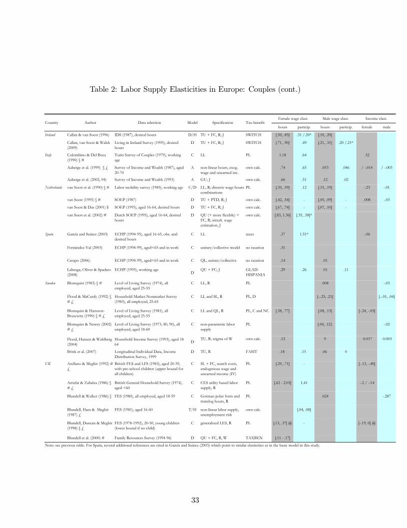
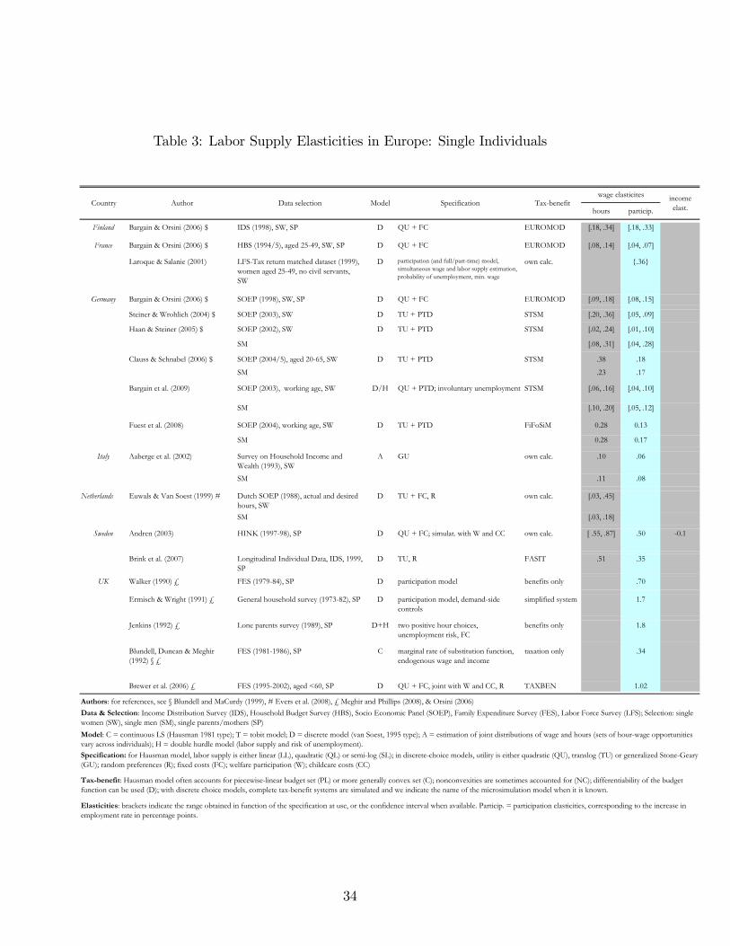
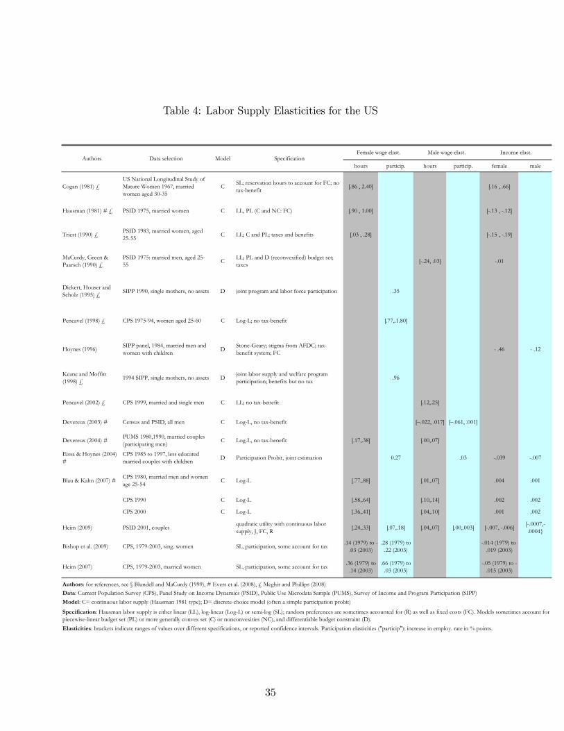
The principal object of examination in this study is the size of wage and income elastic-ities, which are standard representations of labor supply responsiveness and particularlyconvenient when conducting international comparisons. To start with, we present a briefaccount of the available techniques to estimate labor supply, then discuss some of theevidence, reported for European couples in Tables 1 and 2, for European single individu-als in Table 3 and for the US in Table 4.2 This survey essentially distinguishes betweenestimates based on the Hausman approach, discrete-choice models and other methods.We put a certain emphasis on the studies based on discrete models with taxation, as thisis the method we use and because of the skyrocketing number of such studies to analyzepolicies in the recent years. Yet we do not pretend to be exhaustive, simply to give asense of the range of elasticities obtained in the literature for Europe and the US.3 Notice,however, that this survey substantially completes previous reviews, notably Blundell andMaCurdy (1999) and Meghir and Phillips (2008), who concentrate mainly on evidencefrom the Hausman model, for the 1980s and 1990s and for Anglo-Saxon countries.
Arguably, the Hausman approach was most often restricted to the case of piecewiselinear and convex budget sets, hence a partial representation of the e¤ect of tax-bene�tpolicies on household budget constraints. MaCurdy et al. (1990) have also emphasized
2To keep our reference list reasonably short, Tables 1-3 refer, for most of the cited studies, to foursurveys which gather all the exact references.
3Note also that we do not cover dynamic models or other margins than hour/participation (migration,tax evasion, work e¤ort, etc.). Evidence on the elasticities of taxable income, as obtained from naturalexperiments, is surveyed in Meghir and Phillips (2008).
4
that the combination of restrictive functional forms (linear labor supply) and estimationmethods that impose theoretical consistency of the labor supply model everywhere in thesample (global satisfaction of Slutsky conditions) leads to biased estimates and possiblyan overstatement of work incentives (see Heim and Meyer, 2003). In contrast, the discrete-choice approach requires the explicit parameterization of consumption-leisure preferencesas it assumes that labor supply decisions can be reduced to choosing among a discrete setof possibilities (e.g., inactivity, part-time and full-time). Thus, there is no need to restrictpreferences and, in particular, to impose their convexity. In practice, speci�c utilityfunctions are used, and we shall check whether the degree of �exibility makes a di¤erence.The discrete approach also solves several other problems encountered with the Hausmanmethod, which explains its relative success over the years. Firstly, discrete models directlyaccount for both participation and working-time decisions (non-participation is just one ofthe discrete options). This is important, as most of labor supply adjustments occur alongthis margin (Heckman, 1993, Eissa and Hoynes, 1996). Secondly, consumption (disposableincome) needs to be assessed only at certain points of the budget curve so that complextax-bene�t systems, that generate nonlinear budget constraints and nonconvex budgetsets, can easily be dealt with. However, in order to maintain computational feasibility,the number of choices is typically limited to commonly agreed durations of work. Weshall check whether moving closer to the continuous case a¤ects the estimated elasticities(see also Heim, 2009, for a model combining continuous and discrete dimensions). Anarrower discretization may also help to capture peaks which are not necessarily identicalacross countries (i.e., the overtime option in the US) in a cross-country analysis like ours.Thirdly, work costs, which also create nonconvexities, and joint decisions in couples aredealt with in a relatively straightforward way in the discrete approach.4
A crucial aspect is the identi�cation of behavioral parameters. Estimates obtainedwith the Hausman approach are often contaminated by measurement errors (the divisionbias) and by assuming wage exogeneity. That is, unobserved characteristics (e.g., beinga hard-working person) in�uence both wages and work preferences so that estimatesobtained from cross-sectional wage variation across individuals are potentially biased.Arguably, natural experiments based on tax reforms do a better job as they directly
4Discrete models do not solve all the problems, however. One of the remaining issues is the factthat some of the choices may not be available to some people because of institutional constraints orindividual/job characteristics. Due to a lack of information, and the large number of countries in ourstudy, we do not deal with this constraint in an elaborated way �which may limit the comparability of ourresults �but simply account for it through speci�c parameters as explained below. Several studies suggestinteresting ways to circumvent the problem, either by allowing the choice set to vary with individualcharacteristics (Aaberge et al., 1995) or by modeling the degree of captivity, possibly due to institutionalconstraints, to each observed hours alternative (Duncan and Harris, 2002). Several authors also usedesired hours rather than observed hours (e.g., van Soest and Das, 2001).
5
identify responses to exogenous variations in net wages, provided that control groups arewell de�ned or that discontinuities in RD estimations are not due to other factors than thepolicy under study. The recent literature has exploited tax-bene�t reforms of the 1980sand 1990s in the US, and to some extent in the UK, to assess labor supply responsiveness(e.g., US income tax reforms, AFDC/TANF reforms, extension of the EITC or the UKtax credit). Many of these important studies report the e¤ects of reforms � see thesurvey of Holz and Scholz (2003) for the US �but not comparable elasticity measures,so they were not included in our survey (e.g., Bingley and Walker, 1997, Hoynes, 1996,Eissa and Liebman, 1996). Also, most of these reforms concerned families with childrenso that very few estimates are available for childless single individuals, as we can seein Table 4 for the US. Moreover, the lack of important reforms or policy discontinuityin Europe, or the under-use of them by European researcher, is re�ected in Tables 1-3 where most studies are based on the estimation of structural models with taxation(a notable exception is the UK). A few studies use grouped data estimations of thecorrelation between hours/participation and wages over a long period to address theproblem of measurement error in hourly wages (e.g., Devereux, 2004). Discrete modelshold an intermediary position between natural experiments and the Hausman approach.Wage endogeneity problem may exist, yet these models account for nonlinear taxationin household budgets, which may create exogenous variation in net wages across regions,periods of time and demographic groups, and hence improve model identi�cation. Wediscuss this point in detail in the next section.
From Tables 1 and 2, a �rst observation is that early evidence using the Hausmantechnique points to relatively large own-wage elasticities for married women, sometimesclose to 1, or even larger, for instance in early studies for France, Germany, Italy orthe UK. In contrast, recent evidence based on discrete-choice models shows more modestelasticities for this group, in a range between :1 and :5, with some exceptions. Severalexplanations provided in the literature pertain to the arguments made above, including theMaCurdy critique, the fact that �xed costs are ignored or simply that these elasticitieswere collected mainly in the 80s, when female participation was still relatively low inmany countries.5 In Table 4, we observe a similar pattern for the US, with very largeestimates in early studies, including Hausman (1981), and more reasonable elasticities inthe recent studies (hour elasticities ranging between :2 and :4). It should be noted thatestimates are very similar whether they stem from reduced-form estimations (Devereux,2004), natural experiments (Eissa and Hoynes, 2004) or structural models (Heim, 2009).As expected, estimates for married men are much smaller and often not signi�cant or even
5More recent evidence coincides with rising participation rates and a mechanical decline in femaleelasticity, as established for the US in Blau and Kahn (2005) and Heim (2007).
6
negative. There are few exceptions, with more substantial male elasticities in Ireland andfor some of the German studies. Evidence for childless single individuals is very limitedand point to very small elasticities. It is possible that participation responses might bemore signi�cant for low-skilled workers (see suggestive evidence in Eissa and Liebman,1996, and the discussion in section 4). More numerous studies are available concerningsingle mothers. This group has received much attention because of higher risk of povertyand the fact that these women are usually more responsive to �nancial incentives. This iscon�rmed in Table 3, where relatively large elasticities are shown, especially for Sweden,the UK and the US.It is noticeable that studies for a given country sometimes report very di¤erent mag-
nitudes, even when the same method is used. For instance for the US, married women�swage elasticity obtained with the Hausman approach vary from :28 (Triest) to :97 (Haus-man), depending on the constraints put on the model (see the discussion in Heim andMeyer, 2003). For France, estimates for married women are also very high with the basicHausman model, but almost zero when introducing �xed costs (in this case, the modelaccount only for variations in hours, cf., Bourguignon and Magnac, 1990). Estimatesobtained with discrete-choice models are somewhat more comparable from one study tothe next. Yet there are still di¤erences, which are more likely driven by selection criteria(for France, high elasticities are found for families with children in Choné et al., 2003) andthe type of data (administrative data in Laroque and Salanié, 2002, household surveysin Bargain and Orsini, 2006). Speci�cations and modeling choices may however play arole in the discrete approach as well, for instance regarding the treatment of couples (e.g.,male-chauvinistic model in Bargain and Orsini, 2006, joint decisions in Bargain et al.,2009). It is rare to �nd several studies focusing on the same country and using a sim-ilar empirical approach, which would o¤er an interesting con�dence interval (this existsfor Germany, with fairly consistent results for married women, yet relatively contrastedestimates for single women across studies).What can be learned from international comparisons at this stage? Focusing on mar-
ried women, for whom we have the largest number of studies, we can observe that largerelasticities prevail in countries where women�s participation is low. This is particularlytrue for Ireland (see Callan et al., 2009) and Italy (see Aaberge et al., 2002). In contrast,women�s participation is high in Nordic countries and elasticities tend to be fairly small(an exception is Blomquist and Hansson-Brusewitz, 1990, for Sweden, but the authorsexamine data from the 1980s, while more recent evidence by Flood et al., 2004, con�rmsmall hour elasticities for this country). Comparing Italy and Norway/Sweden, Aaberge etal. (2000) show that lower participation rates among married women in Southern Europeleads to a larger potential for reforms that increase �nancial incentives to work. Apartfrom these extreme cases, di¤erences across countries may not be very large, as suggested
7
by Evers et al. (2008). However, comparisons are muddled by all the methodological dif-ferences highlighted above and are incomplete (estimates are missing for several countriesand demographic groups). The remainder of this study aims to �ll some of this gap byestimating labor supply elasticities in a comparable fashion in 17 European countries andthe US and for all demographic groups.
3 A Common Empirical Approach
3.1 Model and Identi�cation
Model and Speci�cation. We essentially follow van Soest (1995), Hoynes (1996) andBlundell et al. (2000) and refer to these studies for more technical details. In our baseline,we specify consumption-leisure preferences using a quadratic utility function, that is, thedeterministic utility of a couple i at each discrete choice j = 1; :::; J can be written as:
Uij = �ciCij + �ccC2ij + �hf iH
fij + �hmiH
mij + �hff (H
fij)2 + �hmm(H
mij )
2 (1)
+�chfCijHfij + �chmCijH
mij + �hmhfH
fijH
mij � Fij
with household consumption Cij and spouses�worked hours Hfij and H
mij . The J choices
of a couple correspond to all combinations of the spouses�discrete hours. Coe¢ cientson consumption and work hours, namely �ci, �hf i and �hmi, are household-speci�c andvary linearly with several taste-shifters (polynomial form of age, presence of children ordependent elders and region). The term �ci also incorporates unobserved heterogeneity forthe model to allow random taste variation and unrestricted substitution patterns betweenalternatives. The �t is improved by the introduction of �xed costs of work as in Callanet al. (2009) or Blundell et al. (2000). Fixed costs explain the fact that there are veryfew observations with a small positive number of worked hours. These costs, denoted Fijand non-zero for positive hour choices, also depend on observed characteristics and areexpressed here in utility metric since they may correspond to actual costs (childcare) orpsychological costs (leaving the children with strangers). They may also capture demand-side constraints and the availability of jobs (see Aaberge et al., 1995). Note that �xed costsare only parametrically identi�ed, i.e., a very �exible utility function could pick up thegap in the distribution at few hours (see van Soest et al., 2002). This militates in favorof relaxing usual regularity conditions on leisure/labor supply (see the methodologicaldiscussion in section 2 and Heim and Meyer, 2003). More generally, as we specify utilitydirectly and not a labor supply function, tangency conditions are not required, and hencewe simply check quasi-concavity of the utility function a posteriori. The only restrictionto our model is the imposition of increasing monotonicity in consumption, which seemsa minimum requirement for meaningful interpretation and policy analysis. Hence, the
8
"structural" aspect of the model is not very constraining, and the restrictions due to thefunctional form can also be relaxed (in the next section, we check the robustness of ourresults to alternative speci�cations). For each labor supply choice j, disposable income(equivalent to consumption in the present static framework) is calculated as a function
Cij = d(wfiH
fij; w
mi H
mij ; yi) (2)
of female earnings, male earnings and non-labor income yi. The tax-bene�t functiond is simulated using calculators that we present in the next section. Male and femalewage rates wfi and w
mi for each household i are predicted using calculated wage rates
from data information on workers and Heckman-corrected wage estimations. Because themodel is nonlinear, the wage-rate prediction errors can be taken explicitly into accountfor a consistent estimation. The deterministic utility is completed by i.i.d. error terms�ij for each choice assumed to represent possible observational errors, optimization errorsor transitory situations. Under the assumption that error terms follow an extreme valuetype I (EV-I) distribution, the (conditional) probability for each household of choosing agiven alternative has an explicit analytical solution (a logistic function of deterministicutilities at all choices). The unconditional probability is obtained by integrating out thedisturbance terms (unobserved heterogeneity and the wage error term) in the likelihood.In practice, this is done by averaging the conditional probability over a large number ofdraws, and the simulated likelihood function can be maximized to obtain all estimatedparameters (Train, 2003).6 The model for single individuals (with or without children) isthe same as above with only one hour term (J is simply the number of discrete optionsfor this person).
Identi�cation. First of all, we predict wages for all observations, as explained above, inorder to reduce some of the bias due to measurement errors on wages stemming from thedivision bias. In addition, accounting fully for tax-bene�t policies helps to create somevariation in net wage between people with the same gross wage. That is, individuals facedi¤erent e¤ective tax schedules, i.e., di¤erent actual marginal tax rates or bene�t with-drawal rates, because of their di¤erent circumstances (di¤erent marital status, age, familycompositions, home-ownership status, disability status) or di¤erent levels of nonlabor in-come. Using nonlinearities and discontinuities generated by the tax-bene�t system in this
6We also insist on the fact that the two-stage approach used here is common practice (see Creedyand Kalb, 2005). Simultaneous estimations of wages and labor supply seem the ideal approach, yetthis approach is rarely adopted (among exceptions, see Laroque and Salanié, 2001). The reason is thattax-bene�t simulations must be run at each iteration of the ML estimation, which requires that they areavailable in the same computer language (this is not the case with EUROMOD) and which also takesmore time (which would not be feasible given the large number of countries we are dealing with).
9
way is a frequent identi�cation strategy in the empirical literature based on static discretemodels and cross-sectional data (see van Soest, 2005, Blundell et al. 2000). Furthermore,we bene�t here from some time and spatial variation that can produce additional exoge-nous variations in net wages. For seven countries, we dispose of two years of data. Thethree-year interval between the two corresponding tax-bene�t systems, 1998 and 2001,gives us some guarantee that enough exogenous changes in tax-bene�t policies occurredover time. Several important reforms indeed took place (e.g., the Working Family TaxCredit reform in the UK, reductions in social security contributions in Belgium and Ger-many, new tax credit and tax reforms, tax reforms in France, Germany, Ireland, etc.,see Orsini, 2006). Notice that consecutive years would provide less exogenous variationbut would also make the assumption of constant preferences over time less restrictive.This trade-o¤ is interesting and rarely discussed in the literature. In the next section,we examine the implications of conducting estimations either on pooled years or on eachyear of data separately.For most countries, we also have regional variation in tax-bene�t rules and, hence, in
net wages. This source of identi�cation has been extensively used in the US (variationsacross states in the income tax code, in bene�ts rules and the EITC are used in laborsupply studies, e.g., Eissa and Hoynes, 2004, Hoynes, 1996, or Meyer and Rosenbaum,2001). For EU member states, housing bene�ts vary in almost all countries at the munici-pality or county level, taking into account local di¤erences in housing costs (exceptions areBelgium, Italy, Portugal and Spain). In Estonia, Hungary and Poland, local governmentsprovide di¤erent supplements to almost all bene�ts, including child bene�ts/allowancesand social assistance. Regional variation in the latter also exists in Denmark, Germany,Italy and Spain. Finally, taxation often varies locally.7 The tax-bene�t simulators at useand demographic information in our datasets allow us to account for all these di¤erencesacross households in our sample. Ideally, of course, one would like to gather many years ofdata for each country to allow for more exogenous variations in net wages (as in Blundellet al., 1998). This is certainly an enormous task when trying to compare many countriesand when accounting for complete tax-bene�t systems, as we do here. Also, we mustacknowledge that the sources of identi�cation are partly di¤erent across countries, which
7County and municipality �at taxes in Nordic countries can vary substantially (ex: 22:8 � 27:8% inDenmark; 16:5 � 21% in Finland; 29 � 36% in Sweden). Regional variations in church tax rates aresigni�cant in Finland and Germany. Note that the mere choice of paying church tax is also a relativelyexogenous variation across individuals in all countries where it exists. Social insurance contributions canvary by region (e.g., in Germany). Other regional variation exists and concerns tax rates (the Nether-lands, Portugal and Spain via imputed rents), tax credits (Belgium), tax deductions (Italy) and counciltaxes (the UK). Note that for the EU, information on tax-bene�t rules for each country is available at:www.iser.essex.ac.uk/research/euromod (together with modeling choices and validation of EUROMOD).For the US, tax-bene�t rules (and TAXSIM) are presented in detail at www.nber.org/~taxsim/.
10
limits the comparability of our results. This issue is obviously not speci�c to our study.In fact, the degree to which we can compare elasticities across studies, most often basedon di¤erent identifying assumptions, could be questioned all the same. We believe thatthe present approach constitutes a reasonable trade-o¤ between comparability attemptand a reasonable identi�cation strategy on cross-sectional data.
Elasticities. In the present nonlinear model, labor supply elasticities cannot be derivedanalytically but can be calculated by numerical simulations using the estimated model.For wage (income) elasticities, we simply predict the change in average work hours andin participation rates following a marginal uniform increase in wage rates (non-laborincome). We have checked that results are similar when wage elasticities are calculatedby simulating either a 1% or a 10% increase in gross wages (unearned incomes). Forcouples, cross-wage elasticities are obtained by simulating changes in female hours whenmale wage rates are increased, and vice versa. For predictions of labor supply e¤ects,baseline estimates rely on the frequency approach, which consists simply of averagingthe probability of each discrete choice over all households before and after a change inwage rates or unearned income. In the robustness section, we also report results usingthe calibration method (Creedy and Kalb, 2005). This approach, consistent with theprobabilistic nature of the model at the individual level, consists of repeatedly drawing aset of J + 1 random terms for each household from an EV-I distribution (together withterms for unobserved heterogeneity), which generate a perfect match between predictedand observed choices. The same draws are kept when predicting labor supply responsesto an increase in wages or non-labor income. Averaging individual responses over a largenumber of draws provides robust transition matrices.
3.2 Data, Selection and Tax-Bene�t Simulations
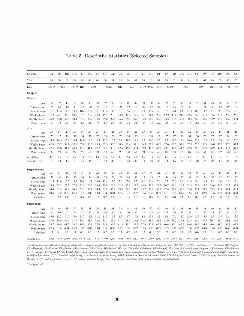
Data and Selection. We focus on the US, 14 members of the EU prior to May 1, 2004(the so-called EU-15 except Luxembourg) and three new member states (NMS), namelyEstonia, Hungary and Poland. For each country, we draw from standard household sur-veys the information about incomes and demographics that can be used for detailedtax-bene�t simulations and labor supply estimations (see data source in the third rowof Table 5). For the EU-15, the datasets at use have been assembled within the frame-work of the EUROMOD project (see Sutherland, 2007) and combined with tax-bene�tsimulations for years 1998, 2001 or both. For the NMS, data were collected for the year2005, and policies simulated for that year, in a more recent development of the EURO-MOD project. For the US, we use the 2006 (Integrated Public Use Microdata Series,IPUMS) Current Population Survey (CPS), which contains information for the year 2005
11
as well. Datasets have been harmonized in the sense that similar income concepts areused together with comparable variable de�nitions. For each country, we extract threesamples (couples, single men and women) for the purpose of labor supply estimations.We only keep households where adults are aged between 18 and 59, available for the labormarket (not disabled, retired or in education) and we exclude self-employed, farmers and"extreme" situations, including very large families and those who report implausibly highlevels of working hours.
Simulations. For each discrete choice j and each household i, disposable income Cij isobtained by adding bene�ts and withdrawing taxes and social contributions to householdgross income. These tax-bene�t calculations, represented by function d() in expression(2), are performed using information on income and socio-demographics together withtax-bene�t simulators. For Europe we use EUROMOD, a calculator designed to simulatethe redistributive systems of the EU-15 countries and of some of the NMS. An introductionto EUROMOD, a descriptive analysis of taxes and transfers in the EU and robustnesschecks are provided by Sutherland (2007). EUROMOD has been used in several empiricalstudies, notably in the comparison of European welfare regimes by Immervoll et al. (2007,2011). For the US, tax-bene�t calculations are conducted using TAXSIM (version v9),the NBER calculator presented in Feenberg and Coutts (1993), augmented by simulationsof social transfers. This calculator is used in combination with CPS data in severalapplications (e.g, Eissa et al., 2008).8 We assume full bene�t take-up and tax compliance.More re�ned estimations accounting for the stigma of welfare program participation wouldrequire precise data information on actual receipt of bene�ts, which is not always availableor reliable in interview-based surveys (see Blundell et al., 2000).
Statistics. Descriptive statistics of the selected samples are presented in Table 5. Formarried women, mean worked hours show considerable variation across countries. Thisis essentially due to lower labor market participation in Southern countries (with thenoticeable exception of Portugal), Ireland and, to a lesser extent, Austria and Poland.The correlation between mean hours and participation rates is :92. There is nonethelesssome variation in work hours among participants, with shorter work duration in Austria,Germany, Ireland, the Netherlands and the UK. The participation of single women is lowerin Ireland and the UK due to the larger frequency of single mothers (we can see that theaverage number of children among single women is the highest in these two countries
8Note that we make use of those policy years available in EUROMOD at the time of writing (1998,2001 or 2005, as indicated above). For comparison, we use TAXSIM simulations for the year 2005.Hopefully, future developments of the EUROMOD project will allow extending our results to more recentdata (and more countries).
12
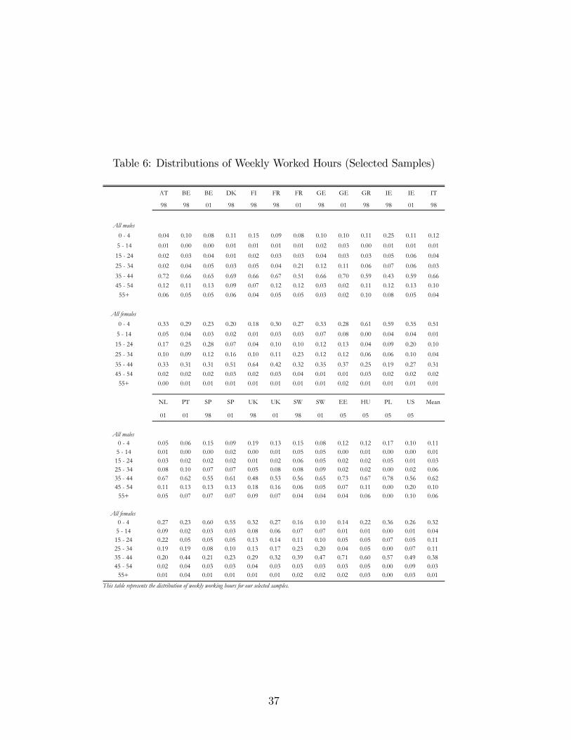
and Poland). There is much less variation for men, the main notable fact being lowerparticipation rate for single compared to married men. The variation in wage rates anddemographic composition across countries is also noteworthy. In particular for marriedwomen, participation rates are correlated with wage rates (corr = :36) and the number ofchildren (�:61). Attached to these patterns, there may be interesting di¤erences acrosscountries in the responsiveness of labor supply to wages and income. We turn to thiscentral issue in the next sections. In Table 6, we take a closer look at the distribution ofactual worked hours. For men, this shows the strong concentration of work hours aroundfull time (35 � 44 hours per week) and non-participation. There is more variations forwomen, in particular with the availability of part-time work in some countries (anotherpeak at 15-24 hours can be seen in Belgium and the Netherlands, or at 25-34 hours inFrance where some �rms o¤er a 3/4 of a full-time contract). The US is characterized by arelatively concentrated distribution (around full-time and inactivity) and a relatively highrate of overtime. To accommodate with the particular hour distribution of each country,while maintaining a comparable framework, we suggest a baseline estimation using a 7-point discretization, i.e., J = 7 for singles and J = 7 � 7 for couples, with choices from0 to 60 hours/week (step of 10 hours). We check below the sensitivity of our results toalternative choice sets.
4 Results
4.1 Labor Supply Estimations
Main Results. Estimated parameters are broadly in line with usual �ndings and wecomment them very brie�y.9 As expected, the presence of children signi�cantly decreasesthe propensity to work for women (both women in couples and single mothers) in mostcountries. Taste shifters related to age are often signi�cant for women in couples but notsystematically for other demographic groups. The constant of the cost of work is alwayssigni�cantly positive for all groups. The presence of young children impact most oftenpositively and signi�cantly on the work cost of women. For single men and women, highereducation leads to lower costs which can be interpreted as demand-side constraints in theform of lower search costs (see van Soest and Das, 2001).
Fit. Pseudo-R2 convey that the �t is reasonably good: :31 on average for couples (:28for singles), from :23 for the UK to :45 for Poland (from :16 in Sweden to :40 in Greecefor single females and :14 in Sweden to :40 in Belgium for single men). Since pseudo-R2
9Due to a lack of space, we do not report estimates. Detailed tables with estimates, log-likelihood andpseudo R2 are available from the authors, separately for couples, single women and single men.
13
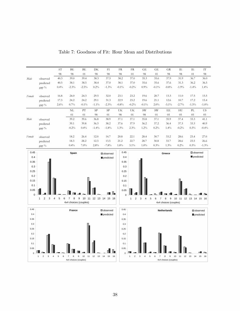
cannot be interpreted as standard R2, a more useful measure of the �t consists of thecomparison between observed and predicted hours. In Table 7, we �rst notice that meanhours compare well, as the discrepancy of mean predicted hours is less than 1% in mostof the cases. There are some exceptions, with larger di¤erences especially for women inPortugal, Greece and Spain. For the two latter countries, we report the distribution ofobserved and predicted frequencies for each choice (here we use 4x4 choices rather than the7x7 baseline, to make it more readable). We can see that the option 11 (both spouses work40 hours/week) is slightly underestimated while the choice 3 (she does not not work, heworks full-time) is overpredicted. Yet, even for these countries, the overall distributionsof observed and predicted hours compare well. We have checked for all countries thatsatisfying comparisons at the mean do not hide wrong hour distributions. We reportonly two additional graphs for an illustration of the case where mean hours are correctlypredicted (France and the Netherlands), con�rming that this corresponds to a situationwhere distributions also compare very well. Finally, we have estimated the baseline modelon a random half of the sample for each country and used it to predict hours for the otherhalf. Fit measures on the holdout sample show good results and convey that the �exiblemodel at use does not over�t the data in a way that would reduce external validity.
4.2 Elasticities
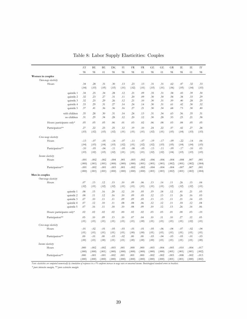
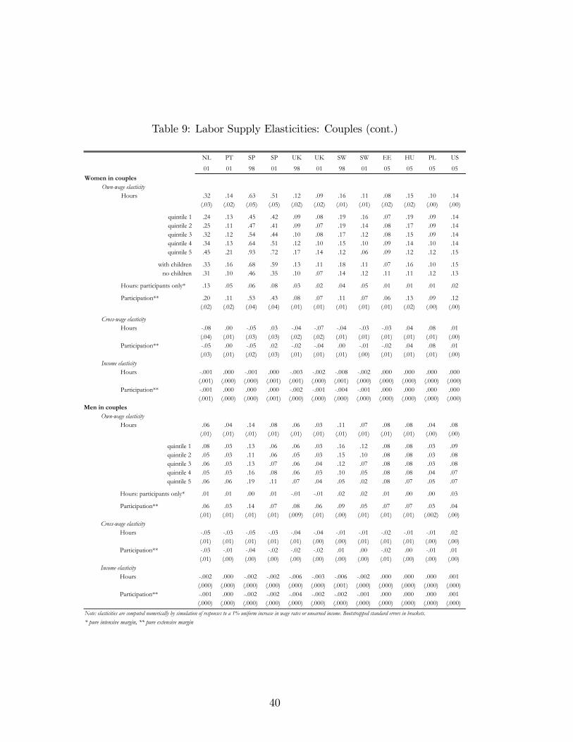
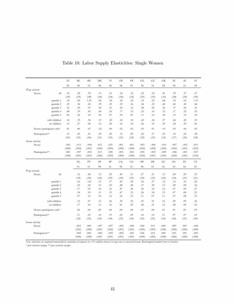
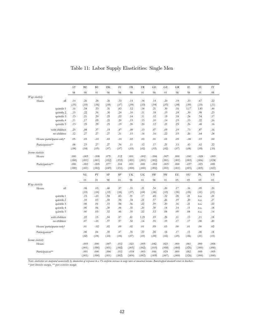
General Comments. Baseline labor supply elasticities are summarized in Tables 8and 9 for couples and Tables 10 and 11 for single women and single men respectively.We report own-wage hour elasticities, overall and for quintiles of disposable income, thehour elasticity for the sub-group of participants (the pure intensive margin) and theparticipation elasticity (the extensive margin), followed by cross-wage hour elasticities andincome elasticities. Bootstrapped standard errors are obtained by repeated random drawsof the model parameters from their estimated distributions and by recalculating elasticitiesfor each draw. This is computationally demanding and we perform these bootstraps onlyfor the main elasticity results. It transpires that estimates are relatively precise, slightlymore for couples than for single individuals.10 Results are broadly in line with stylizedfacts in this literature. Firstly, most of the response to wage changes is due to changes inparticipation (the extensive margin). The pure intensive elasticities are extremely smallfor all countries and all demographic groups, for example, lower than :08 for marriedwomen in all countries (except the Netherlands). They are sometimes negative for men in
10This may be due to the fact that there is less variation in labor market behavior among singles (withthe exception of lone parents when compared to childless single individuals). Also, the model for couplesgenerally �ts the data better because the relatively high level of voluntary inactivity among marriedwomen conforms well with the supply-side behavioral assumptions.
14
couples (Italy and the UK) and for singles (for instance, single men in Belgium, Irelandand Portugal). Reassuringly, the total (own-wage) hour elasticity is close to the sum ofthe pure intensive elasticity and the participation elasticity in most of the cases. Secondly,own-wage elasticities are the largest for married women and the smallest for married men,as expected. For couples, cross-wage elasticities are negative and smaller than own-wageelasticities, yet nonetheless sizeable for some countries (Austria, Denmark, Germany andIreland), which is not an usual result (see, e.g., Callan et al., 2009, or Aaberge et al., 2000).As often in the literature, income elasticities are negative and very small in absolute value.Blundell and MaCurdy (1999) report that variation between studies regarding the incomeelasticity appears to be greater than the corresponding variation with respect to thewage elasticity. We do not con�rm much variation as far as "controlled" cross-countrycomparisons are concerned. In the following, we focus speci�cally on own-wage elasticitiesto link our results to the existing literature.
Reconciliation with Past Results. The survey in section 2 conveyed the idea thatelasticities are relatively modest when estimated using unconstrained, discrete-choicemodels (as compared to �rst generation Hausman models). Our results con�rm thistrend in a more de�nitive manner, given the large number of countries under investiga-tion and the common framework at use. Concerning married women, our estimates arevery close to, or not statistically di¤erent from, past �ndings for Austria, Belgium, Fin-land, Germany, Sweden and the UK.11 Our estimates are however smaller or close to thelower bound of past con�dence intervals for Ireland, Italy and the Netherlands, which ispartly explained by the use of older data in the cited studies based on discrete models(e.g., papers by van Soest and coauthors cited in Table 2) or by a di¤erent, more generalapproach where the choice set is extended to hour-wage bundles (see papers by Aaberge,Colombino and coauthors in Table 2). For France, elasticities for married women aresmaller than in other studies, which can be attributed to di¤erent methods, data andselection as explained above. For Spain, our estimates are relatively large compared toprevious evidence, yet the rare studies based on discrete models do not report con�denceintervals. Our estimates for the US are very small and compare well to the most recentresults (Heim, 2009). US studies which report larger elasticities rely on older data, whileit has been shown that elasticities have dramatically decreased over time (Heim, 2007).For other countries, evidence based on discrete models is not directly comparable to ourresults or simply absent. For other demographic groups, the comparison is even more lim-ited. Our estimates for married men compare well to previous results in countries where
11For instance for Germany, most studies report median own-wage elasticities of around :3 for marriedwomen (with relatively broad con�dence intervals), which is similar to our result for the years 1998 and2001.
15
signi�cant evidence exist (Belgium, Germany, Ireland, Italy, the Netherlands, Sweden andthe US), but comparison points for other countries are generally missing. The situationis similar in the case of single individuals. There is a substantial number of estimates forGermany, with which our results conform well. In the case of single mothers, numerousstudies on single mothers are available on the UK and the US. Our results point to moremoderate elasticities than in most of these studies, mainly for the data year and method-ology reasons discussed above, with the exception of Blundell et al. (1992) for the UK andDickert et al. (1995) for the US, which report comparable estimates to ours. Our resultsnicely complete the scattered evidence in the literature by providing a comprehensive andmore comparable assessment of EU-US elasticities. We discuss them in detail, beforeturning back to our initial questions: how do elasticities compare across countries?
New Results and International Comparisons We �rst focus on married women,the group mostly studied in the literature. For them, hour and participation elasticitiesare to be found in a very narrow range :2 � :3 for several countries (Austria, Belgium,Denmark, Germany, Italy and the Netherlands). They are slightly smaller, around :1� :2,but signi�cantly di¤erent from zero in France (for 2001), Finland, Portugal, Sweden, theNMS, the UK and the US. They are signi�cantly larger, between :4 and :6, in Ireland,Greece and Spain. Total hour elasticities follow the same pattern. Thus, our resultsshow that elasticities are relatively modest and hold in a narrow interval once comparabledatasets, selection and empirical strategies are used. This is an interesting result given thesubstantial di¤erences that exist across countries in terms of labor market conditions, in-stitutions and preferences/culture. Notice that estimates are su¢ ciently precise, however,so that di¤erences between the three groups of countries mentioned above are statisticallysigni�cant. The nature of the remaining di¤erences between countries is investigated inthe next section. Note that the simple intuition that elasticities are larger when femaleparticipation is lower is broadly con�rmed by the data, i.e., the cross-country correlationbetween mean wage hour (participation) elasticities and mean worked hours (participationrates) is around �0:81 (�0:84). For married men, results are even more compressed, withown-wage elasticities usually ranging between around :05 and :15. Estimates are usuallysigni�cantly larger than zero and precise enough to �nd statistical di¤erences across somecountries, yet less pronounced than for women. The correlation between elasticities andworked hours (participation) is only around �0:41 (�0:64). Elasticities for single menshow a little more variation, usually in a range between 0 and :3 with a few exceptions(estimates are signi�cantly higher in Ireland and Spain). They are signi�cantly di¤erentfrom zero in most cases with some exceptions including Italy and Portugal. Estimates areslightly larger than for married men overall, which is in line with lower participation ratesamong singles. We also observe some variation among single women, usually between :1
16
and :4 with larger elasticities for some countries (around :6 in Belgium and Italy). Thecorrelation between elasticities and worked hours (participation) among single individualsis usually smaller than for couples: :50 (:50) for women and :32 for men (:46).
Other Dimensions. In Tables 8-11, we provide additional results beyond simple meanelasticities. For single individuals and married men, the distribution of elasticities acrossincome groups (quintiles) shows a clear decreasing pattern, with largest elasticities forlow-income groups. In fact, heterogeneous elasticity across di¤erent earnings groups iscrucial for welfare analysis. Eissa et al. (2008) show that normative conclusions of pol-icy evaluations change completely when recognizing that participation elasticities can besigni�cantly larger at the bottom of the distribution. Very few studies report this kindof information however (see evidence based on structural models in Meghir and Phillips,2008, for the UK and Aaberge et al., 2002, for Italy). Interestingly, our results general-ize their �ndings for single individuals and, to some extent, for married men. Results formarried women do not show such a pattern, which has to do with joint decision in couples�Eissa (1995) also �nds that elasticities for married women may still be substantial atthe top.For couples and single women, we also report estimates for those with and without
children. In Table 10, we notice that single mothers tend to have larger elasticities thanchildless women, yet di¤erences are usually not signi�cant. The notable exceptions, withvery large elasticities for single mothers, concern Greece and Ireland. The same resultis observed for married couples: elasticities are usually larger for women with children,but not markedly. The main exceptions are Greece, Ireland and Spain, i.e., the high-elasticity group for married women.12 Finally, when two years of data are available, wehave reported elasticities based on separate estimations for each year. Time variationis small but seems to coincide with smaller elasticities when participation increases overtime. We also �nd that estimates of the utility function are relatively similar across years,which is reassuring about the fact that preferences do not change substantially over thethree-year interval. Yet they may change enough to explain time change in elasticities.As discussed above, identi�cation is improved when two years of data are pooled. Inthat case, i.e., when assuming identical preferences for the two years, we �nd almostidentical elasticities for the two years, which broadly correspond to the average of thetwo elasticities reported in Tables 8-11. For instance, we �nd own-wage elasticities ofaround :18 for married women in France for both 1998 and 2001. This con�rms that time12Table 5 shows that the number of couples with children is large in Ireland but close to average in
Greece and Spain. Hence, higher elasticities among married women in these countries do not seem to bedriven by a higher proportion of families with children but by the higher responsiveness of mothers. Thisis con�rmed by the decomposition analysis in the next section.
17
di¤erences observed in Tables 8-11 are due to (small) changes in preferences over timerather than other factors like changes in demographic characteristics. This is line withthe results of Heim (2007), for the US, over a much longer time period.
4.3 Robustness Checks
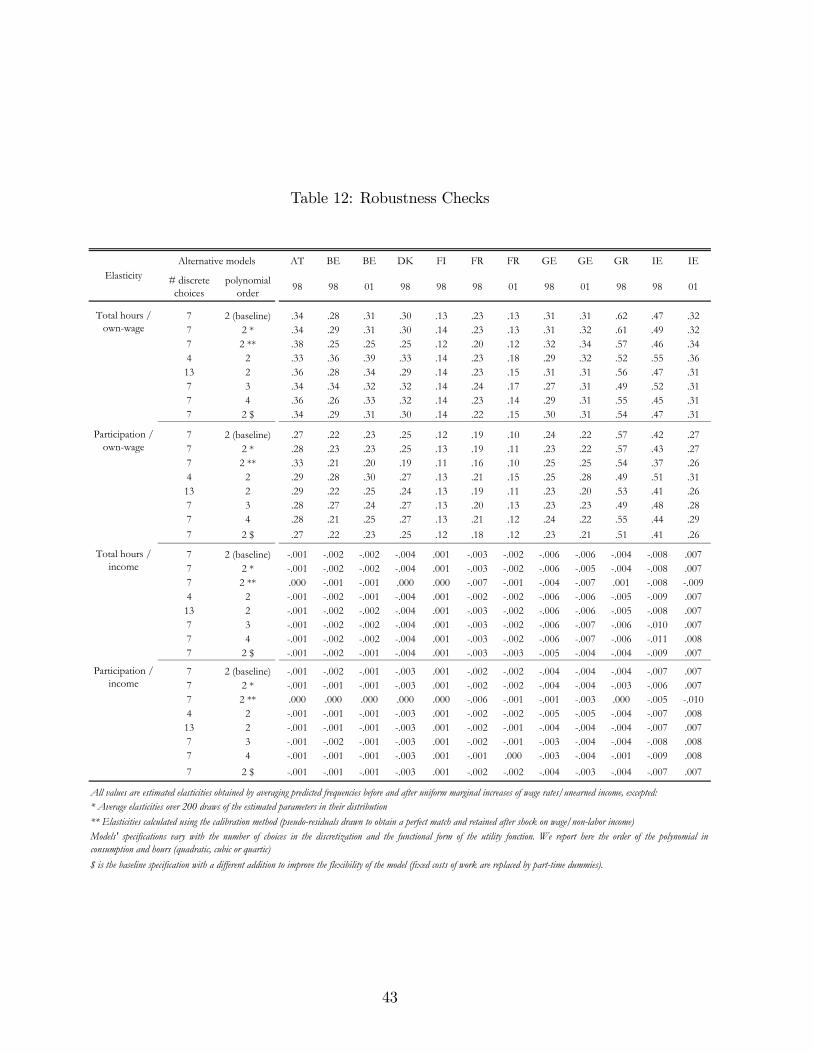
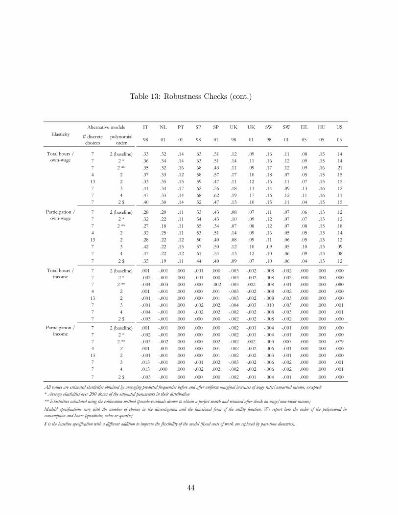
We have argued that models with discrete choices are very general as they do not requireimposing much constraint on preferences and allow accounting for complete tax-bene�tpolicies a¤ecting household budgets. As discussed in Section 2, we may nonetheless checkwhether our estimates are sensitive to several crucial aspects of the model speci�cation.Results of this extensive robustness check are provided in Tables 12 and 13 where wefocus on the own-wage and income elasticities of total hours and participation for marriedwomen. Firstly, we simply check the sensitivity to the method used to calculate elas-ticities. The �rst row of results corresponds to the baseline, that is, a 7-choice modelwith quadratic utility and �xed costs, whereby elasticities are obtained by the frequencymethod. The second row reports the average elasticity over the 250 draws used to boot-strap standard errors in the baseline model. The third row shows elasticities obtainedwith the calibration method, as previously de�ned. Reassuringly, we see very little di¤er-ences in the three sets of results. Secondly, and more importantly, we check whether themain restriction of the model, i.e., the fact that the choice set is discretized, plays somerole. The next rows in each panel report elasticities when alternative choice sets are used,namely a discretization with 4� and 13�hour choices. The model with J = 4 choices forsingles (4 � 4 = 16 for couples) essentially captures the commonly agreed durations ofwork: non-participation (0), part-time (20), full-time (40) and overtime (50 hours/week).Such a model does not adapt particularly well to the hour distribution of each country.The narrower discretization with 13 choices, from 0 to 60 hours/week with a step of 5hours, and 13� 13 = 169 combinations for couples, is more computationally demanding.However, it may capture more country-speci�c hour distributions and, in fact, get closerto a continuous speci�cation. Interestingly, Tables 12 and 13 show that results are verysimilar in all three cases (J = 4; 7 and 13). Only slightly larger elasticities are observed inthe 4-point case for some countries (e.g., Belgium and Ireland). Finally, we check whetherelasticities are sensitive to the functional form at use. Similar to van Soest et al. (2001)for the Netherlands, we experiment alternative speci�cations by increasing the order ofthe polynomial in the utility function: quadratic (baseline) then cubic and quartic. Wealso change the way �exibility is gained in the model by replacing �xed costs of work,as used in Blundell et al. (2000), by part-time dummies, precisely at the 10, 20 and30 hour choices, as used in van Soest (1995). These parameters may be interpreted asjob search costs for less common working hours (van Soest and Das, 2001), and hence
18
include some of the labor market restriction on the choice set. Results for these di¤erentspeci�cations are shown in the last rows of each panel in Tables 12 and 13. The size ofelasticities hardly changes across the di¤erent modeling choices.13 This result reinforcesour main conclusions regarding international comparison. Given the large number ofcountries involved, this extensive sensitivity check also adds signi�cantly to the literatureby increasing con�dence in the use of discrete models.
5 Assessing the Cross-Country Di¤erences
The evidence presented above suggests that some cross-country di¤erence in labor supplyelasticities remains after controlling for di¤erences in the empirical approach, the sampleselection and when focusing on a relatively narrow time period. Fully explaining cross-country di¤erences in labor supply and labor supply responsiveness is of course beyondthe scope of this paper.14 In this section, however, we attempt to isolate several importantfactors. We still focus on married women, primarily because this group shows the mostsigni�cant variation in elasticities across countries.
5.1 Wage and Labor Supply Levels
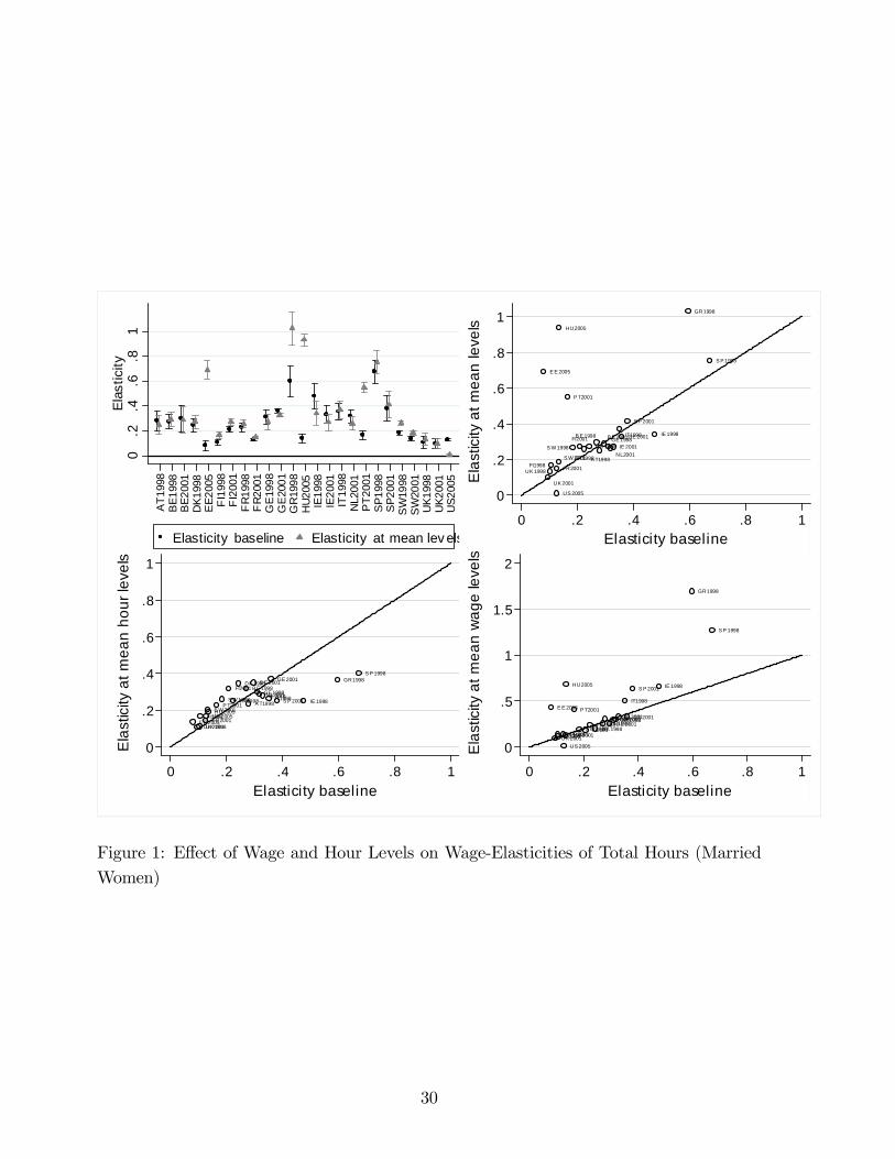
We have seen that hour and participation elasticities are strongly correlated with meanhour and participation levels across countries. It is possible, then, that larger elasticitiesin countries like Greece, Ireland and Spain are not due to behavioral parameters butinstead to the hour and wage levels that enter the formal de�nition of elasticities, i.e.,�c =
@Hc@wc
wcHcfor country c. To probe the e¤ect of these variables and their di¤erence across
countries, we compute elasticities as �Mc = @Hc@wc
wH, using country-speci�c responsiveness
@Hc@wc
and holding hour and wage levels at their mean values over all countries (accountingfor PPP di¤erences for wages). We focus on own-wage elasticities of total hours and reportthe results in Figure 1. The upper left panel compares elasticities in the baseline (circles)and in the "mean levels" scenario (triangular) together with 95% bootstrapped con�dence
13The only exception seems to be Italy where higher order polynomial utility leads to larger elasticities.The di¤erence with the baseline is statistically signi�cant only in the case of participation elasticities, andpartly disappears when we restrict the condition of participation to people working at least �ve hours aweek when calculating elasticities (indeed, there are a number of initial non-working women for whomthe predicted number of weekly hours is very small after the wage increase used to calculate elasticities�the additional restriction is reasonable if we consider that it is unusual to observe such small values).14A long list of of studies have addressed this issue, sometimes in a more comprehensive manner than
in the present framework, for instance by accounting simultaneously for labor supply and fertility choices(e.g., the recent study by Michaud and Tatsiramos, 2011). Yet no de�nitive answer has been brought tothis di¢ cult question of country di¤erences in working time and participation.
19
intervals. The two scenarios are plotted one against the other in the upper right panel.Lower panels decompose the "mean levels" scenario into two sub-scenarios, one whereonly hours are hold at the international mean value H (lower left) and one where onlythe mean wage level w (lower right) is used. Results show that high-elasticity countrieslike Greece and Spain are not only characterized by lower female participation but alsoby lower wage rates, so that these countries remain in the high-elasticity group even inour "mean levels" scenario. This mechanical exercise also pushes Estonia, Hungary andPortugal in the high-elasticity group while it reduce US elasticities to the lowest level.This is clearly due to the fact that the NMS and Portugal (the US) have signi�cant lower(higher) wage rates while their female participation rates are close to the internationalaverage. Despite these notable exceptions, the upper right panel of Figure 1 shows thatcross-country di¤erences are preserved when elasticities are evaluated at mean values andmust therefore be explained by other factors.
5.2 Tax bene�t Systems
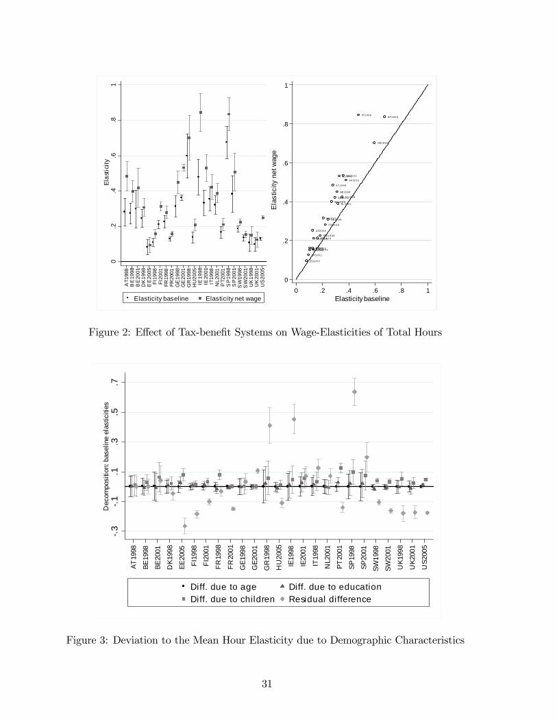
There are many reasons why accounting for tax-bene�t policies is important in our study:(i) labor supply estimates are often used to simulate policy reforms; (ii) nonlinearity ine¤ective marginal tax rates and how they vary with individual characteristics (familycomposition and unearned incomes) aids in identifying the model; (iii) a model ignoringtaxes may be misspeci�ed. In addition, the size of hour elasticities may be in�uenced bydi¤erences in tax-bene�t systems across countries. Precisely, the responsiveness capturedby the derivative @Hc=@wc is calculated in our base estimates by incrementing gross wagesby 1%. In this way, the fact that high tax countries, like in the North of Europe, arecharacterized by smaller net wage increments could explain smaller elasticities. To checkthis point, we simulate a 1% increase in the net wage, in order to cancel out di¤erencesin e¤ective marginal tax rates (EMTR) across countries due to di¤erent tax schedulesor bene�t withdrawal rates.15 Figure 2 reports total hour elasticities in the baselineand in this "net-wage increment" scenario. The right panel plots the two situations whilethe left panel additionally indicate the 95% bootstrapped con�dence intervals. In general,elasticities after a 1% increase in net wage are larger �indeed a 1% changes in gross wagescorrespond to smaller increments due to taxation. However, and most importantly, cross-country variation is barely a¤ected when accounting for di¤erences in implicit taxation
15This is done by retrieving the EMTR on earnings of each individual in the household (tf ; tm) as well asEMTR on unearned income (ty) using the tax-bene�t calculators. In other words, we numerically linearize(2) to express disposable income, for each choice j, as Cj = wf (1� tf )Hf
j +wm(1� tm)Hm
j + (1� ty)y.With a truly linear tax system, a 1% increase in gross and net wage is equivalent. With nonlinear taxsystems, we account for the change in tf occurring when gross wage rates are increased, in order tosimulate exactly a 1% increase in the net female wage wf (1� tf ).
20
of labor income. Since tax-bene�t systems can also a¤ect hours and participation, and,in this way, the size of elasticities, we have also simulated a scenario where existing tax-bene�t systems are withdrawn completely (or, alternatively, replaced by a uniform �attax system, which yields similar conclusions). With this counterfactual, the three groupsof countries still emerge as the main trend and con�rm that "natural" di¤erences exist atleast across these broad groups which are not due to tax-bene�t institutions.
5.3 Demographic Characteristics
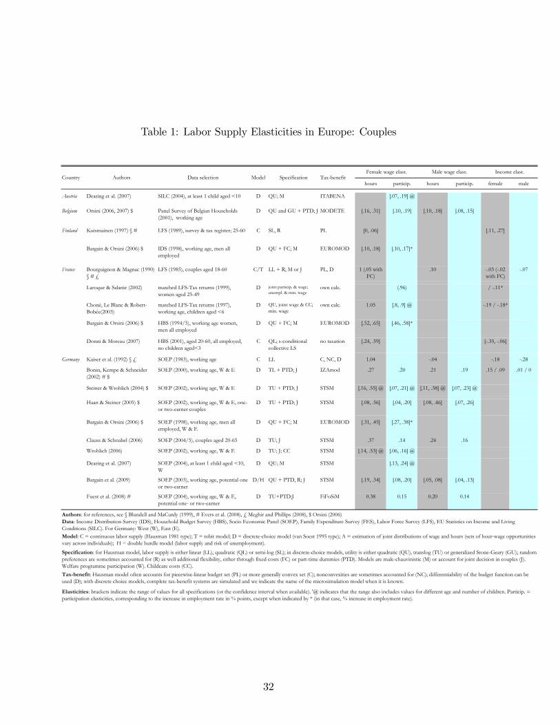
We �nally turn to the role of demographic composition. As indicated in Section 3.2,important di¤erences exist across countries in this respect, notably the number of childrenbut also the age and education structure. It is plausible that these demographic di¤erenceshave an e¤ect on the size of elasticities. To investigate this point, we decompose di¤erencesin elasticities across countries using an approach similar to that in Heim (2007). Let idenote a woman�s age cohort, j her education group and k the number of her children.16
Let �ijk;c denote the wage elasticity of total hours for a woman of type ijk in country c. Themean elasticity in this country, �c, can be written as a weighted average
Pi
Pj
Pk
Pijk;c�ijk;c;
where Pijk;c denotes the proportion of women of type ijk in this country. This proportioncan be re-written as Pijk;c = Pi;cPjji;cPkjij;c where Pi;c denotes the proportion of womenin age cohort i in country c, Pjji;c the proportion of women in education group j givenmembership in age cohort i, and Pkjij;c denotes the proportion of women with k childrengiven membership in age cohort i and education group j. Letting P denote the meanproportion of a certain type over all countries, the proportion Pijk;c can be expressed as:
Pijk;c = P iP jjiP kjij +�Pi;c � P i
�P jjiP kjij (3)
+Pi;c�Pjji;c � P jji
�P kjij + Pi;cPjji;c
�Pkjij;c � P kjij
�:
This expression can be used to decompose the mean elasticity where �ijk denotes the meanelasticity for type ijk over all countries:
�c =
Xi
Xj
Xk
P iP jjiP kjij�ijk
!+
Xi
Xj
Xk
�Pi;c � P i
�P jjiP kjij�ijk
!(4)
+
Xi
Xj
Xk
Pi;c�Pjji;c � P jji
�P kjij�ijk
!+
Xi
Xj
Xk
Pi;cPjji;c�Pkjij;c � P kjij
��ijk
!
+
Xi
Xj
Xk
Pi;cPjji;cPkjij;c (�ijk;c � �ijk)!:
16In our application, we retain three age groups (aged 18-35, 36-45, and 45-59), two education groupsand three family sizes (no children, 1-2 children, 3 children or more). Re�ning with three educationgroups leads to too many empty cells.
21
The decomposition starts with the overall mean weighted elasticity, a term common to allcountries. The next term denotes how elasticities vary due to the di¤erent composition ofage cohorts, keeping the distributions of education and family size constant within an agegroup. The variation in elasticities due to di¤erent education levels, keeping the distrib-ution of the number of children within education levels constant, is captured in the thirdcomponent. The fourth term indicates the di¤erence in elasticities due to di¤erent distri-butions of family size. The last component denotes the di¤erence in elasticities left to beexplained by di¤erent elasticities within an age-education-children cell, which can be inter-preted as a residual di¤erence due to other factors than composition e¤ects (for instance,di¤erences in preferences). The results of this decomposition are presented in Figure 3.We show the deviation of the country-speci�c elasticities from the mean elasticity thatcan be attributed to di¤erences pertaining to each of the three demographic factors aswell as the residual, unexplained di¤erence. It turns out that di¤erences in demographiccomposition regarding age and education are never statistically signi�cant. Variation infamily size contributes very slightly to larger elasticities in some countries, including Es-tonia, France, Ireland, Portugal and Spain. Yet these di¤erences are signi�cant only in afew cases, and certainly do not explain the bulk of country di¤erences. Once controllingfor these composition e¤ects, the residual term corresponding to "overall" di¤erences inlabor supply responsiveness shows a signi�cantly positive e¤ect for Greece, Ireland andSpain (the high-elasticity group) and a signi�cantly negative e¤ect for Finland, France,Sweden, the UK and the US (the low-elasticity group). Therefore, we must concludethat di¤erences in demographic compositions between countries are not responsible forvariations in labor supply elasticities.17
5.4 Alternative Explanations
This leaves room for other explanations. Firstly, there may be genuine di¤erences inwork preferences, possibly due to long-lasting di¤erences in culture and the norms vis-a-vis female labor market participation. Secondly, and in a related way, social preferencesmay vary across countries and lead to di¤erent institutions, notably regarding childcarearrangements. It may be the case that di¤erences in some of the estimated parame-ters, and in particular the �xed costs of work, re�ect country heterogeneity vis-a-visnon-simulated policies like childcare support. Di¤erence in industrial or occupationalcomposition may also play a role, as employment in France and the Nordic countries isoften reported to be more stable due to better work-family reconciliation policies. Thedata at hand do not allow probing such di¤erences across countries and we leave this for
17We have checked that alternative decomposition paths �given the path dependency of the method �give similar results. Similar conclusions are also obtained when using the "net wage" elasticities.
22
future research. Finally, an explanation in terms of selection can be put forward. We �ndthat marriage rates are signi�cantly higher in high-elasticity countries (the proportionof married women over single women is 6:3 in Ireland or 5:6 in Spain, compared to anaverage of 3:9 over all countries under study). Hence, it could be that married women inthese countries cover a large range of the distribution of elasticities while the relativelysmaller fraction of women who marry in France, the Nordic countries, the UK and theUS are in the low range of this distribution. If this was the case, one would expect to �ndlarger elasticities among single women in the latter group of countries. Our main resultsshow that it is not the case �the cross-country correlation between elasticities of marriedand single women is positive (:25) �so this possible explanation can be ruled out.
6 Conclusions
The present paper presents new evidence on labor supply elasticities for 17 Europeancountries and the US. Estimates are more comparable than usual results in the literaturegiven the e¤ort of adopting a common empirical approach. The main lesson from theresults is that elasticities are more modest than usually thought, and international di¤er-ences are relatively small. We also show that the remaining variation across countries haslittle to do with selection into marriage, di¤erences in tax-bene�t systems or heterogene-ity in demographic composition. It may rather re�ect di¤erences in individual and socialpreferences across countries, and primarily di¤erences in work preferences and childcarepolicies, as captured by variation in labor supply parameters. As far as married womenare concerned, these di¤erences contribute to more intermittent labor force participationpatterns in Greece, Ireland and Spain as opposed to more consistent participation andmore constant hours in other countries and notably France, the Nordic countries, the UKand the US. This result corroborates the �ndings of Heim (2007) regarding time variationof elasticities in the US.18
Future work should consider both time and country variation. The present study wasbased on data years for which policy simulations were available within EUROMOD, yetfuture research should attempt to span a longer period for many countries. Also, a bettermodeling of demand-side constraints could improve the results, which was not possiblewith the data at hand. The bias concerns primarily single individuals, for whom the shareof involuntarily unemployment is the highest, but not so much married women and singlemothers, two groups who frequently choose non-participation on a voluntary basis due to
18Considering time rather than cross-country variation, Heim (2007) also �nds that higher participationrates coincide with much smaller elasticities, and that this trend is not due to demographic changes butmore likely to shifts in work preferences.
23
�xed costs of work and preferences (see Bingley andWalker, 1997, and Bargain et al., 2006,for an extensive analysis of biases a¤ecting elasticities in that case). A more comprehensivemeasure of elasticities would also account for the interaction between demand and supply(see Peichl and Siegloch, 2010) or for general equilibrium e¤ects.Despite these restrictions, we believe that the estimates provided in this paper can be
useful for researchers who want to implement optimal tax or CGE models in a compara-tive framework and need to refer to "reasonable" values from the literature (e.g., Jacobs,2009, on reassessing Prescott�s argument). In particular, our results can be exploited forapplications in the �eld of taxation (see also Blundell et al., 2008). Two recent studies,Immervoll et al. (2007 and 2011), have conducted international comparisons of redistrib-utive systems in Europe and their results could be reassessed in the light of the estimatesprovided in the present study. Firstly, Immervoll et al. (2007) measure the implicitcost of redistribution using plausible elasticities and sensitivity analyses �but withoutinformation on actual cross-country di¤erences. Secondly, they assume that participationelasticity decreases with income levels. The implications of this assumption are crucial forwelfare analysis (Eissa et al., 2008). Notably, the optimality of policies that support theworking poor, compared to traditional "demogrant" policies, depends fundamentally onit. While very limited evidence exists, the present study broadly supports this assumptionfor single individuals and married men, providing a precise range of estimates for eachcountry. Thirdly, international comparisons of the tax treatment of couples by Immervollet al. (2011) �essentially the long-studied issue of joint versus individual taxation �couldbe reevaluated using our new evidence on couples�labor supply elasticities. Related tothis point, Heckman (1993) noted "whether labor supply behavior by sex will convergeto equality as female labor-force participation continues to increase is an open question".This question has remained open up to now, and the present study contributes to answer-ing it. In fact, we can draw from our results that male-female di¤erentials in participationrates are strongly negatively correlated with male-female di¤erentials in participation elas-ticities (corr = �:89).19 Hence, the Ramsey argument against high implicit taxation ofsecondary earners and the subsequent deadweight loss from joint "e¤ective" taxation �which is more frequent than mere joint taxation since many bene�ts and tax credits aremeans-tested on household income � can now be assessed on the basis of comparableestimates for many countries.
19In Nordic countries, the gender participation gap is below 10 points and coincides with insigni�cantdi¤erences in labor supply elasticities. In Spain or Greece, men�s participation is still above women�s bya large margin (around 50 points) and the gender di¤erence in elasticities is signi�cant and larger than:45. Most EU countries and the US are somewhere between these two extreme cases.
24
References
[1] Aaberge, R., J. Dagsvik and S. Strom (1995): �Labor supply responses and welfaree¤ects of tax reforms�, Scandinavian Journal of Economics, 97(4), 635-59.
[2] Aaberge, R., U. Colombino and S. Strøm (2000): �Labor supply responses and welfaree¤ects from replacing current tax rules by a �at tax: empirical evidence from Italy,Norway and Sweden�, Journal of Population Economics, 13, 4, 595-621.
[3] Aaberge R., Colombino U. and T. Wennemo (2002): "Heterogeneity in the elasticityof labour supply in Italy and some policy implications", WP CHILD #21/2002.
[4] Andrén, T. (2003): "A Structural Model of Childcare, Welfare, and the Labor Supplyof Single Mothers", Labour Economics, 10(2), 133-147.
[5] Ballard, C., J. Shoven and J. Whalley (1985): "General Equilibrium Computations ofthe Marginal Welfare Costs of Taxes in the United States", American EconomicReview, 75(1), pp. 128�137.
[6] Bargain, O. and K. Orsini (2006): "In-work policies in Europe: Killing two birdswith one stone?", Labour Economics 13, 667�697
[7] Bargain, O., Caliendo, M., Haan, P., Orsini, K. (2009): "�Making Work Pay� in aRationed Labour Market", Journal of Population Economics, 23(1), 323-351
[8] Bingley, P. and I. Walker (1997): �The Labour Supply, Unemployment and Partic-ipation of Lone Mothers in In-Work Transfer Programmes�, Economic Journal,107, 1375-1390
[9] Blau, F. and L. Kahn (2007): "Changes in the Labor Supply Behavior of MarriedWomen: 1980�2000". Journal of Labor Economics, 25, pp. 393�438.
[10] Blomquist, S., and U. Hansson-Brusewitz (1990): "The E¤ect of Taxes on Male andFemale Labor Supply in Sweden", Journal of Human Resources, 25, 317-357.
[11] Blundell, R., Duncan, A. and Meghir, C. (1998): "Estimating Labour Supply Re-sponses Using Tax Reforms", Econometrica 66(4)(4): 827�861.
[12] Blundell, R. and T. MaCurdy (1999): �Labor Supply: A Review of AlternativeApproaches�, in Ashenfelter and Card (eds), Handbook of Labor Economics ,vol.3A, ch.27, Elsevier North-Holland.
[13] Blundell, R., A. Duncan, J. McCrae and C. Meghir (2000): �The Labour MarketImpact of the Working Families�Tax Credit�, Fiscal Studies, 21, 1, 75-103.
[14] Blundell, R., M. Brewer, P. Haan and A. Shephard (2008): "Optimal income taxationof lone mothers: an empirical comparison for Germany and the UK", EconomicJournal, 119, 535, 101-121
25
[15] Bourguignon, F. and T. Magnac (1990): �Labour supply and taxation in France�,Journal of Human Resources, 25, 358-389.
[16] Bovenberg, A. L., J.J. Graa�and and R.A. de Mooij (2000): "Tax reform and theDutch labor market : an applied general equilibrium approach", Journal of PublicEconomics, 78, 193-214.
[17] Bishop, K., B. Heim, K. Mihaly(2009): "Single Women�s Labor Supply Elasticities:Trends and Policy Implications," Industrial and Labor Relations Review, 63(1),146-168
[18] Brink, A., K. Nordblom and R.Wahlberg (2007) �Maximum Fee versus Child Bene�t:A Welfare Analysis of Swedish Child-Care Fee Reform�, International Tax andPublic Finance, Vol.14 (4), 457-480.
[19] Callan, T., A. van Soest, J. Walsh (2009): "Tax Structure and Female Labour Supply:Evidence from Ireland", Labour, 23(1), 1-35
[20] Chetty, R., J. Friedman, T. Olsen and L. Pistaferri (2009): "The e¤ect of adjustmentcosts and institutional constraints on labor supply elasticities: evidence fromDenmark", Working Paper.
[21] Choné, P., D. Le Blanc and I. Robert-Bobée (2003): �Female labor supply and childcare in France�, CREST working paper.
[22] Clauss, M. and R. Schnabel (2006): "Distributional and Behavioural E¤ects of theGerman Labour Market Reform", ZEW working paper.
[23] Creedy, J. and G. Kalb (2005): "Discrete hours labour supply modelling: speci�ca-tion, estimation and simulation", Journal of Economic Surveys, 19(5), 697-733
[24] Crespo, L. (2006): "Estimation and Testing of Household Labour Supply Models:Evidence from Spain", mimeo
[25] Dearing, H., H. Hofer, C. Lietz, R. Winter-Ebmer, K. Wrohlich (2007): "Why AreMothers Working Longer Hours in Austria than in Germany? A ComparativeMicrosimulation Analysis", Fiscal Studies, 28 (4), 463�495
[26] Devereux, P. (2004): "Changes in RelativeWages and Family Labor Supply", Journalof Human Resources, 39, 696�722.
[27] Dickert, S., S. Houser and J.K. Scholz (1995): �The Earned Income Tax Credit andTransfer Programs: A Study of Labor Market and Program Participation.�in J.Poterba (ed.), Tax Policy and the Economy 9th ed., 1-50.
[28] Duncan, A. and M. N. Harris (2002): "Intransigencies in the Labour Supply Choice",Melbourne Institute Working Paper No 17/02,
26
[29] Eissa, N. (1995). Taxation and Labour Supply of Married Women: The Tax ReformAct of 1986 as a Natural Experiment. NBER Working Paper No. 5023
[30] Eissa, N. and H. W. Hoynes (2004): "Taxes and the labor market participation ofmarried couples: the earned income tax credit," Journal of Public Economics,vol. 88 (9-10), pages 1931-1958.
[31] Eissa, N. and Liebman, J. (1996): "Labor supply response to the earned income taxcredit", Quarterly Journal of Economics 111(2): 605�637.
[32] Eissa, N., H. J. Kleven, C.T. Kreiner (2008): "Evaluation of Four Tax Reforms in theUnited States: Labor Supply and Welfare E¤ects for Single Mothers", Journal ofPublic Economics 92, 795�816
[33] Evers, M., R. de Mooij, D. van Vuuren (2008): "The wage elasticity of labour supply:a synthesis of empirical estimates", De Economist, 156:25�43
[34] Feenberg, D. and E. Coutts (1993): "An Introduction to the TAXSIM Model", Jour-nal of Policy Analysis and Management, 12(1)
[35] Fernández-Val, I. (2003): "Household Labor Supply: Evidence for Spain", Investiga-ciones Económicas, 27(2), 239-275.
[36] Flood, L., J. Hansen & R. Wahlberg (2004): �Household Labour Supply and WelfareParticipation in Sweden�, Journal of Human Ressources, 39 (4), 1008-1032.
[37] Fuchs, V.R., A. B. Krueger and J. M. Poterba (1998): "Economists�Views about Pa-rameters, Values, and Policies: Survey Results in Labor and Public Economics",Journal of Economic Literature, 36(3), 1387-1425
[38] García, I. and M.J. Suárez (2003): "Female labour supply and income taxation inSpain: The importance of behavioural assumptions and unobserved heterogeneityspeci�cation", Revista de Economía Pública, 164(1): 9-27
[39] Hausman, J. (1981): �Labor Supply�, in How Taxes A¤ect Economic Behavior, ed.H.Aaron and J.Pechman, The Brookings Institution, Washington D.C., 27-72.
[40] Hausman, J. (1985): �Taxes and labour Supply�in Handbook of Public Economics,ed. Auerbach and Feldstein, Amsterdam, North-Holland.
[41] Heckman, J. (1993): "What has be learned about the labor supply in the past twentyyears", American Economic Review, Papers and Proceedings, 83, 116-121.
[42] Heim, B. and B. Meyer (2003): "Work costs and nonconvex preferences in the esti-mation of labor supply models", Journal of Public Economics, 88(11)2323-38
[43] Heim, B. (2007): �The Incredible Shrinking Elasticities: Married Female Labor Sup-ply, 1978�2002.�Journal of Human Resources 42(4): 881�918.
27
[44] Heim, B. (2009): �Structural Estimation of Family Labor Supply with Taxes: Esti-mating a Continuous Hours Model Using a Direct Utility Speci�cation.�Journalof Human Resources 44(2): 350�385.
[45] Hoynes, H. W. (1996): �Welfare transfers in two-parent families: Labor supply andwelfare participation under AFDC-UP�, Econometrica, 64(29), 295-332.
[46] Immervoll, H., H. J. Kleven, C. T. Kreiner and E. Saez (2007): �Welfare reform inEuropean countries: a microsimulation analysis�, Economic Journal, 117, 1 - 44.
[47] Immervoll, H., H. J. Kleven, C. T. Kreiner and N. Verdelin (2011): "An Evalua-tion of the Tax-Transfer Treatment of Married Couples in European Countries",forthcoming, Journal of Public Economics.
[48] Jacobs, B. (2009): "Is Prescott right? Welfare state policies and the incentives towork, learn, and retire", International Tax Public Finance, 16: 253�280
[49] Killingsworth, M., and J. Heckman (1986): "Female labor supply: a survey". In: O.Ashenfelter and R. Layard, eds., Handbook of Labor Economics, vol. I, North-Holland, Amsterdam, pp.103-204.
[50] Kimmel, J. and T. J, Kniesner (1998): "New Evidence on Labor Supply: Employ-ment Versus Hours Elasticities by Sex and Marital Status." Joumal of MonetaryEconomics 42(2), 289-30L
[51] Kydland, F. E. (1995): "Business Cycles and Aggregate Labor Market Fluctuations,"In Frontiers of Business Cycle Research, ed. Thomas F, Cooley, 126-56. Princeton.N. J.: Princeton University Press.
[52] Labeaga, J.M., X. Oliver and A. Spadaro (2008): �Discrete choice models of laboursupply, behavioural microsimulation and the Spanish tax reform�, Journal ofEconomic Inequality, 6(3), 247-273.
[53] Laroque, G. and B. Salanié (2001): �Labor market, institutions and employment inFrance�, Journal of Applied Econometrics, 17, 25-48.
[54] MaCurdy, T., P. Green, and H. Paarsch (1990): "Assessing Empirical Approaches forAnalyzing Taxes and Labor Supply", Journal of Human Resources, 25, 415-490.
[55] Meghir, C. and D. Phillips (2008): "Labour Supply and Taxes", Institute for FiscalStudies, WP 08/04.
[56] Meyer, B. and Rosenbaum, D. (2001): "Welfare, the earned income tax credit, andthe labor supply of single mothers", Quarterly Journal of Economics 116(3):1063�1114.
28
[57] Mo¢ tt, R. (1990), Introduction to the Special Issue on Taxation and Labor Supplyin Industrial Countries, Journal of Human Resources, 25(3), 313-316
[58] Orsini, K. (2006): �Tax bene�t reforms and the labor market: Evidence from Belgiumand other EU countries�, Leuven University, working paper.
[59] Peichl, A. and Siegloch, S. (2010): "Accounting for Labor Demand E¤ects in Struc-tural Labor Supply Models", IZA Discussion Paper 5350.
[60] Pencavel, J.H. (1986): �Labor supply of men: a survey�, in O. Ashenfelter and R.Layard (eds), Handbook of Labor Economics, vol.1, Amsterdam, North-Holland.
[61] Prescott, E.C. (2004): "Why do Americans work so much more than Europeans?,"Quarterly Review, Federal Reserve Bank of Minneapolis, issue Jul, 2-13.
[62] Saez, E. (2001): �Using elasticities to derive optimal income taxe rates�, Review ofEconomic Studies, 68, 205-229.
[63] Smith, N., S. Dex, J.D. Vlasblom and T. Callan (2003): �The e¤ects of taxation onmarried women�s labour supply across four countries�, Oxford Economic Papers,55, 3, 417-439
[64] Sutherland, H. (2007): "Euromod: the tax-bene�t microsimulation model for theEuropean Union", in A. Gupta and A. Harding (eds), Modelling Our Future:Population Ageing, Health and Aged Care, Vol. 16 of International Symposia inEconomic Theory and Econometrics, Elsevier, pp. 483�488.
[65] Michaud, P.-C. and K. Tatsiramos (2011): "Fertility and Female Employment Dy-namics in Europe: The E¤ect of Using Alternative Econometric Modeling As-sumptions", forthcoming in Journal of Applied Econometrics
[66] Train, K. (2003). Discrete Choice Models using Simulation. Cambridge, UK: Cam-bridge University Press.
[67] van Soest, A. (1995): �Structural Models of Family Labor Supply: a Discrete ChoiceApproach�, Journal of Human Resources, 30, 63-88.
[68] van Soest, A. and M. Das (2001): �Family labor supply and proposed tax reforms inthe Netherlands�, De Economist, 149(2), 191-218.
[69] van Soest, A., M. Das and X.Gong (2001): �A structural labor supply model withnon-parametric preferences�, Journal of Econometrics (Annals), 107, 345-374.
29
0.2
.4.6
.81
Elas
ticity
AT1
998
BE1
998
BE2
001
DK1
998
EE2
005
FI1
998
FI2
001
FR1
998
FR2
001
GE
1998
GE
2001
GR
1998
HU2
005
IE19
98IE
2001
IT19
98N
L200
1P
T200
1S
P199
8S
P200
1S
W19
98S
W20
01U
K199
8U
K200
1U
S200
5
Elasticity baseline Elasticity at mean lev els
A T1998
B E 1998 B E 2001
DK 1998
E E 2005
FI1998
FI2001
FR1998
FR2001
GE 1998GE 2001
GR1998
HU2005
IE 1998
IE 2001
IT1998
NL2001
P T2001
S P 1998
S P 2001
S W 1998
S W 2001
UK 1998
UK 2001
US 20050
.2
.4
.6
.8
1
Ela
stic
ity a
t mea
n le
vels
0 .2 .4 .6 .8 1Elasticity baseline
A T1998
B E 1998B E 2001DK 1998
E E 2005FI1998
FI2001
FR1998
FR2001
GE 1998
GE 2001 GR1998
HU2005
IE 1998IE 2001IT1998
NL2001
P T2001
S P 1998
S P 2001S W 1998
S W 2001
UK 1998UK 2001
US 2005
0
.2
.4
.6
.8
1
Ela
stic
ity a
t mea
n ho
ur le
vels
0 .2 .4 .6 .8 1Elasticity baseline
A T1998B E 1998B E 2001
DK 1998
E E 2005
FI1998FI2001
FR1998
FR2001
GE 1998GE 2001
GR1998
HU2005 IE 1998
IE 2001
IT1998
NL2001
P T2001
S P 1998
S P 2001
S W 1998S W 2001UK 1998
UK 2001US 20050
.5
1
1.5
2
Ela
stic
ity a
t mea
n w
age
leve
ls
0 .2 .4 .6 .8 1Elasticity baseline
Figure 1: E¤ect of Wage and Hour Levels on Wage-Elasticities of Total Hours (MarriedWomen)
30
0.2
.4.6
.81
Elas
ticity
AT1
998
BE
1998
BE
2001
DK
1998
EE
2005
FI19
98FI
2001
FR19
98FR
2001
GE
1998
GE
2001
GR
1998
HU
2005
IE19
98IE
2001
IT19
98N
L200
1P
T200
1S
P19
98S
P20
01S
W19
98S
W20
01U
K19
98U
K20
01U
S20
05
Elasticity baseline Elasticity net wage
AT 19 9 8
BE19 9 8
BE20 0 1
DK19 9 8
EE20 0 5
F I1 9 9 8
F I2 0 0 1
F R19 9 8
F R20 0 1
GE19 9 8
GE20 0 1
GR19 9 8
HU20 0 5
IE1 9 9 8
IE2 0 0 1
IT 1 9 9 8
NL 20 0 1
PT 20 0 1
SP19 9 8
SP20 0 1
SW 1 9 9 8
SW 2 0 0 1UK19 9 8
UK20 0 1
US20 0 5
0
.2
.4
.6
.8
1
Ela
stic
ity n
et w
age
0 .2 .4 .6 .8 1Elasticity baseline
Figure 2: E¤ect of Tax-bene�t Systems on Wage-Elasticities of Total Hours
.3.1
.1.3
.5.7
Dec
ompo
sitio
n: b
asel
ine
elas
ticiti
es
AT19
98
BE19
98
BE20
01
DK1
998
EE20
05
FI19
98
FI20
01
FR19
98
FR20
01
GE1
998
GE2
001
GR
1998
HU
2005
IE19
98
IE20
01
IT19
98
NL2
001
PT20
01
SP19
98
SP20
01
SW19
98
SW20
01
UK1
998
UK2
001
US2
005
Diff. due to age Diff. due to educationDiff. due to children Residual difference
Figure 3: Deviation to the Mean Hour Elasticity due to Demographic Characteristics
31
Table 1: Labor Supply Elasticities in Europe: Couples
hours particip. hours particip. female male
Austria Dearing et al. (2007) SILC (2004), at least 1 child aged <10 D QU; M ITABENA [.07, .19] @
Belgium Orsini (2006, 2007) $ Panel Survey of Belgian Households(2001), working age
D QU and GU + PTD; J MODETE [.16, .31] [.10, .19] [.10, .18] [.08, .15]
Finland Kuismainen (1997) § # LFS (1989), survey & tax register; 2560 C SL, R PL [0, .06] [.11, .27]
Bargain & Orsini (2006) $ IDS (1998), working age, men allemployed
D QU + FC; M EUROMOD [.10, .18] [.10, .17]*
France Bourguignon & Magnac (1990)§ # £
LFS (1985), couples aged 1860 C/T LL + R; M or J PL, D 1 (.05 withFC)
Fuest et al. (2008) # SOEP (2004), working age, W & E,potential one or twoearner
D TU+PTD;J FiFoSiM 0.38 0.15 0.20 0.14
Authors: for references, see § Blundell and MaCurdy (1999), # Evers et al. (2008), £ Meghir and Phillips (2008), $ Orsini (2006)
TaxbenefitIncome elast.Female wage elast. Male wage elast.
Model SpecificationCountry Authors Data selection
Elasticities: brackets indicate the range of values for all specifications (or the confidence interval when available). '@ indicates that the range also includes values for different age and number of children. Particip. =participation elasticities, corresponding to the increase in employment rate in % points, except when indicated by * (in that case, % increase in employment rate).
Data: Income Distribution Survey (IDS), Household Budget Survey (HBS), Socio Economic Panel (SOEP), Family Expenditure Survey (FES), Labor Force Survey (LFS), EU Statistics on Income and LivingConditions (SILC). For Germany: West (W), East (E).Model: C = continuous labor supply (Hausman 1981 type); T = tobit model; D = discretechoice model (van Soest 1995 type); A = estimation of joint distributions of wage and hours (sets of hourwage opportunitiesvary across individuals); H = double hurdle model (labor supply and risk of unemployment).
Specification: for Hausman model, labor supply is either linear (LL), quadratic (QL) or semilog (SL); in discretechoice models, utility is either quadratic (QU), translog (TU) or generalized StoneGeary (GU); randompreferences are sometimes accounted for (R) as well additional flexibility, either through fixed costs (FC) or parttime dummies (PTD). Models are malechauvinistic (M) or account for joint decision in couples (J).Welfare programme participation (W). Childcare costs (CC).Taxbenefit: Hausman model often accounts for piecewiselinear budget set (PL) or more generally convex set (C); nonconvexities are sometimes accounted for (NC); differentiability of the budget function can beused (D); with discrete choice models, complete taxbenefit systems are simulated and we indicate the name of the microsimulation model when it is known.
32
Table 2: Labor Supply Elasticities in Europe: Couples (cont.)
FES (19781992), 2050, young children(lower bound if no child)
C generalized LES, R PL [.13, .37] @ [.19, 0] @
Blundell et al. (2000) # Family Resources Survey (199496) D QU + FC, R, W TAXBEN [.11 .17]
Note: see previous table. For Spain, several additional references are cited in García and Suárez (2003) which point to similar elasticities as in the basic model in this study.
Model SpecificationCountry Author Data selection TaxbenefitIncome elast.Female wage elast. Male wage elast.
33
Table 3: Labor Supply Elasticities in Europe: Single Individuals
hours particip.
Finland Bargain & Orsini (2006) $ IDS (1998), SW, SP D QU + FC EUROMOD [.18, .34] [.18, .33]
France Bargain & Orsini (2006) $ HBS (1994/5), aged 2549, SW, SP D QU + FC EUROMOD [.08, .14] [.04, .07]
Bargain et al. (2009) SOEP (2003), working age, SW D/H STSM [.06, .16] [.04, .10]
SM [.10, .20] [.05, .12]
Fuest et al. (2008) SOEP (2004), working age, SW D TU + PTD FiFoSiM 0.28 0.13
SM 0.28 0.17
Italy Aaberge et al. (2002) Survey on Household Income andWealth (1993), SW
A own calc. .10 .06
SM .11 .08
Netherlands Euwals & Van Soest (1999) # Dutch SOEP (1988), actual and desiredhours, SW
D own calc. [.03, .45]
SM [.03, .18]
Sweden Andren (2003) HINK (199798), SP D QU + FC; simulat. with W and CC own calc. [ .55, .87] .50 0.1
Brink et al. (2007) Longitudinal Individual Data, IDS, 1999,SP
D TU, R FASIT .51 .35
UK Walker (1990) £ FES (197984), SP D participation model benefits only .70
Ermisch & Wright (1991) £ General household survey (197382), SP D participation model, demandsidecontrols
simplified system 1.7
Jenkins (1992) £ Lone parents survey (1989), SP D+H two positive hour choices,unemployment risk, FC
benefits only 1.8
Blundell, Duncan & Meghir(1992) § £
FES (19811986), SP C marginal rate of substitution function,endogenous wage and income
taxation only .34
Brewer et al. (2006) £ FES (19952002), aged <60, SP D QU + FC, joint with W and CC, R TAXBEN 1.02
Authors: for references, see § Blundell and MaCurdy (1999), # Evers et al. (2008), £ Meghir and Phillips (2008), & Orsini (2006)
incomeelast.
wage elasticitesCountry Author Data selection Model Specification Taxbenefit
TU + FC, R
TU + PTD
QU + PTD; involuntary unemployment
Elasticities: brackets indicate the range obtained in function of the specification at use, or the confidence interval when available. Particip. = participation elasticities, corresponding to the increase inemployment rate in percentage points.
Model: C = continuous LS (Hausman 1981 type); T = tobit model; D = discrete model (van Soest, 1995 type); A = estimation of joint distributions of wage and hours (sets of hourwage opportunitiesvary across individuals); H = double hurdle model (labor supply and risk of unemployment).Specification: for Hausman model, labor supply is either linear (LL), quadratic (QL) or semilog (SL); in discretechoice models, utility is either quadratic (QU), translog (TU) or generalized StoneGeary(GU); random preferences (R); fixed costs (FC); welfare participation (W); childcare costs (CC)
Taxbenefit: Hausman model often accounts for piecewiselinear budget set (PL) or more generally convex set (C); nonconvexities are sometimes accounted for (NC); differentiability of the budgetfunction can be used (D); with discrete choice models, complete taxbenefit systems are simulated and we indicate the name of the microsimulation model when it is known.
Data & Selection: Income Distribution Survey (IDS), Household Budget Survey (HBS), Socio Economic Panel (SOEP), Family Expenditure Survey (FES), Labor Force Survey (LFS); Selection: singlewomen (SW), single men (SM), single parents/mothers (SP)
GU
34
Table 4: Labor Supply Elasticities for the US
hours particip. hours particip. female male
Cogan (1981) £US National Longitudinal Study ofMature Women 1967, marriedwomen aged 3035
C SL; reservation hours to account for FC; notaxbenefit [.86 , 2.40] [.16 , .66]
Hausman (1981) # £ PSID 1975, married women C LL, PL (C and NC: FC) [.90 , 1.00] [.13 , .12]
Triest (1990) £ PSID 1983, married women, aged2555 C LL; C and PL; taxes and benefits [.03 , .28] [.15 , .19]
MaCurdy, Green &Paarsch (1990) £
PSID 1975: married men, aged 2555 C LL; PL and D (reconvexified) budget set;
taxes [.24, .03] .01
Dickert, Houser andScholz (1995) £ SIPP 1990, single mothers, no assets D joint program and labor force participation .35
Pencavel (1998) £ CPS 197594, women aged 2560 C LogL; no taxbenefit [.77,.1.80]
Hoynes (1996) SIPP panel, 1984, married men andwomen with children D StoneGeary; stigma from AFDC; tax
benefit system; FC .46 .12
Keane and Moffitt(1998) £ 1994 SIPP, single mothers, no assets D joint labor supply and welfare program
participation; benefits but no tax .96
Pencavel (2002) £ CPS 1999, married and single men C LL; no taxbenefit [.12,.25]
Devereux (2003) # Census and PSID, all men C LogL, no taxbenefit [–.022, .017] [–.061, .001]
Devereux (2004) # PUMS 1980,1990, married couples(participating men) C LogL, no taxbenefit [.17,.38] [.00,.07]
Eissa & Hoynes (2004)#
CPS 1985 to 1997, less educatedmarried couples with children D Participation Probit, joint estimation 0.27 .03 .039 .007
Blau & Kahn (2007) # CPS 1980, married men and womenage 2554 C LogL [.77,.88] [.01,.07] .004 .001
CPS 1990 C LogL [.58,.64] [.10,.14] .002 .002
CPS 2000 C LogL [.36,.41] [.04,.10] .001 .002
Heim (2009) PSID 2001, couples quadratic utility with continuous laborsupply, J, FC, R [.24,.33] [.07,.18] [.04,.07] [.00,.003] [.007, .006] [.0007,
.0004}
Bishop et al. (2009) CPS, 19792003, sing. women SL, participation, some account for tax .14 (1979) to .03 (2003)
.28 (1979) to.22 (2003)
.014 (1979) to .019 (2003)
Heim (2007) CPS, 19792003, married women SL, participation, some account for tax .36 (1979) to.14 (2003)
.66 (1979) to.03 (2003)
.05 (1979) to .015 (2003)
Authors: for references, see § Blundell and MaCurdy (1999), # Evers et al. (2008), £ Meghir and Phillips (2008)
Elasticities: brackets indicate ranges of values over different specifications, or reported confidence intervals. Participation elasticities ("particip"): increase in employ. rate in % points.
Income elast.
Data: Current Population Survey (CPS), Panel Study on Income Dynamics (PSID), Public Use Microdata Sample (PUMS), Survey of Income and Program Participation (SIPP)Model: C= continuous labor supply (Hausman 1981 type); D= discretechoice model (often a simple participation probit)
Specification: Hausman labor supply is either linear (LL), loglinear (LogL) or semilog (SL); random preferences are sometimes accounted for (R) as well as fixed costs (FC). Models sometimes account forpiecewiselinear budget set (PL) or more generally convex set (C) or nonconvexities (NC), and differentiable budget constraint (D).
Selected sample: household with workingage adults (either employed, unemployed or inactive). For this table and the following ones: Policy years are 1998, 2001 or 2005; Countries are: AT=Austria, BE=Belgium,DK=Denmark, FI=Finland, FR=France, GE=Germany, GR=Greece, IE=Ireland, IT=Italy, NL=the Netherlands, PT=Portugal, SP=Spain, UK=the United Kingdom, SW=Sweden, EE=Estonia,HU=Hungary, PL=Poland, US=the United States. Reported years correspond to the period when income information was collected. Datasets are: ECHP=European Community Household Panel, PSB=Panel Surveyon Belgian Households, HBS=Household Budget Survey, IDS=Income Distribution Survey, SOEP=German or Dutch SocioEconomic Panel, LIS=Living in Ireland Survey, SHIW=Survey of Households Income andWealth, FES=Family Expenditure Survey, CPS=Current Population Survey. Hourly wage rates are converted in 2001 euros (predicted for nonparticipants).
PSB HBS SOEP LIS ECHP IDSFES
36
Table 6: Distributions of Weekly Worked Hours (Selected Samples)
Note: elasticities are computed numerically by simulation of responses to a 1% uniform increase in wage rates or unearned income. Bootstrapped standard errors in brackets.* pure intensive margin, ** pure extensive margin
Note: elasticities are computed numerically by simulation of responses to a 1% uniform increase in wage rates or unearned income. Bootstrapped standard errors in brackets.* pure intensive margin, ** pure extensive margin
Note: elasticities are computed numerically by simulation of responses to a 1% uniform increase in wage rates or unearned income. Bootstrapped standard errors in brackets.* pure intensive margin, ** pure extensive margin
Note: elasticities are computed numerically by simulation of responses to a 1% uniform increase in wage rates or unearned income. Bootstrapped standard errors in brackets.* pure intensive margin, ** pure extensive margin
All values are estimated elasticities obtained by averaging predicted frequencies before and after uniform marginal increases of wage rates/unearned income, excepted:* Average elasticities over 200 draws of the estimated parameters in their distribution** Elasticities calculated using the calibration method (pseudoresiduals drawn to obtain a perfect match and retained after shock on wage/nonlabor income)
$ is the baseline specification with a different addition to improve the flexibility of the model (fixed costs of work are replaced by parttime dummies).
Models' specifications vary with the number of choices in the discretization and the functional form of the utility fonction. We report here the order of the polynomial inconsumption and hours (quadratic, cubic or quartic)