Labor Supply Heterogeneity and Demand for Child Care of Mothers with Young Children Patricia Apps Sydney University Law School and IZA JanKab´atek* Tilburg University and Netspar Ray Rees CES, University of Munich Arthur van Soest Tilburg University and Netspar February 23, 2012 Abstract This paper introduces a static structural model of hours of market labor supply, time spent on child care and other domestic work, and bought in child care for married or cohabiting mothers with pre-school age children. The father’s behavior is taken as given. The main goal is to analyze the sensitivity of hours of market work, parental child care, other household production and formal child care to the wage rate, the price of child care, taxes, benefits and child care subsidies. To account for the non-convex nature of the budget sets and, possibly, the household technology, a discrete choice model is used. The model is estimated using the HILDA dataset, a rich household survey of the Australian population, which contains detailed information on time use, child care demands and the corresponding prices. Simulations based on the estimates show that the time allocations of women with pre-school children are highly sensi- tive to changes in wages and the costs of child care. A policy simulation suggests that labor force participation and hours of paid work would in- crease substantially in a fiscal system based solely on individual rather than joint taxation. JEL classification: J22, J13, H24 Keywords: Time use, income tax, child care subsidies *Corresponding author: Department of Econometrics & OR, Tilburg University, P.O. Box 90153, 5000 LE Tilburg, The Netherlands. Email: [email protected]. Preliminary version 1
Transcript
Labor Supply Heterogeneity and Demand for
Child Care of Mothers with Young Children
Patricia AppsSydney University Law School and IZA
Jan Kabatek*Tilburg University and Netspar
Ray ReesCES, University of Munich
Arthur van SoestTilburg University and Netspar
February 23, 2012
Abstract
This paper introduces a static structural model of hours of marketlabor supply, time spent on child care and other domestic work, andbought in child care for married or cohabiting mothers with pre-schoolage children. The father’s behavior is taken as given. The main goal isto analyze the sensitivity of hours of market work, parental child care,other household production and formal child care to the wage rate, theprice of child care, taxes, benefits and child care subsidies. To accountfor the non-convex nature of the budget sets and, possibly, the householdtechnology, a discrete choice model is used. The model is estimated usingthe HILDA dataset, a rich household survey of the Australian population,which contains detailed information on time use, child care demands andthe corresponding prices. Simulations based on the estimates show thatthe time allocations of women with pre-school children are highly sensi-tive to changes in wages and the costs of child care. A policy simulationsuggests that labor force participation and hours of paid work would in-crease substantially in a fiscal system based solely on individual ratherthan joint taxation.
JEL classification: J22, J13, H24Keywords: Time use, income tax, child care subsidies
*Corresponding author: Department of Econometrics & OR, TilburgUniversity, P.O. Box 90153, 5000 LE Tilburg, The Netherlands. Email:[email protected].
Preliminary version
1
1 Introduction
One of the most striking, and still largely unexplained, facts about female laborsupply in the developed countries is its heterogeneity across households, andindeed across countries. In most OECD countries, on average around one-thirdof women work full time in the labor force, one third do various amounts of parttime work, and one third work solely in household production. Very little of theaggregate heterogeneity across all households in any one country is explained bywage rate differences and by the number of children present in the household.Moreover, the correlation between female labor supply and fertility across thesecountries is strongly positive, even though historically, in any one country, therehas been an inverse relationship between them.
Some insight is gained by organizing the data in terms of life cycle phasesbased on the number and age of children in the household. In the pre-childrenphase, there is very little difference between male and female labor supply distri-butions. This changes dramatically when children enter the household, and thisis when the female labor supply heterogeneity essentially sets in. Though thereis a trend of return to the labor force over subsequent phases of the life cycleas the children reach school age and beyond, the basic pattern of heterogeneitypersists. Such findings suggest that for the theoretical and empirical analysisof the female labor supply heterogeneity it would be fruitful to focus on the lifecycle phase in which the household makes its labor supply decisions in the pres-ence of young children. However, in order to do so, it is important to be awareof idiosyncratic characteristics which are common among these households.
Clearly, the birth of a child represents a fundamental change in the livesof the parents. Childbearing affects the couple’s preferences, consumption pat-terns, and it is particularly demanding in terms of their time. The neccessityto nurture and educate the young child leads parents either to specialize in self-provision of childcare, or to rely on services provided by other caregivers suchas relatives, friends, or formal institutions.
Sufficient provision of childcare is essential for proper development of thechildren, and as such, it is bound to have profound impact on the mother’sdecision making, especially in terms of labor force participation. The importanceof the availability and the cost of childcare services has been confirmed bya host of both theoretical (Apps & Rees 2009) and empirical studies1 of thefemale labor supply. And for that reason, we consider careful treatment of themothers’ childcare-related decisions to be one of the key aspects of female laborsupply modeling.
This paper presents a static structural discrete choice model analyzing thetime allocation choices of married and cohabiting mothers with pre-school aged
1Previous works on labor supply and childcare decisions include Ribar (1995),Duncan et al. (2001), Blau (2003), Connelly & Kimmel (2003), Doiron & Kalb (2005),Kalenkoski et al. (2005), Kornstad & Thoresen (2007), Baker et al. (2008), and Blundell& Shepard (2011).
2
children2. The main advantage of the discrete choice approach is that it canaccount for the non-convex nature of the household budget sets and, possi-bly, also of the household technology. Within the model, we analyze mother’sdecisions about her hours of market work, time spent on childcare and otherdomestic work, and amount of bought-in childcare. The main goal is to assessthe sensitivity of choices at the intensive and extensive margin of the female la-bor supply, and to capture underlying substitution patterns between alternativeuses of mothers’ time.
Unlike previous studies, we allow the household utility to take on more flex-ible functional form (following Van Soest (1995) and Van Soest & Stancanelli(2010)). We also embody both formal and informal childcare directly into thehousehold utility function3. The key innovation of our approach is however theincorporation of unobserved heterogeneity in the flexible form of latent classes4.We choose to extend the treatment of unobserved heterogeneity beyond thetraditional framework of random coefficient models5, as the assumptions im-posed on the stochastic parameter components may well prove unrealistic inthe context of female labor supply.
The reliability of random coefficient models hinges on the assumption thatthe latent heterogeneity is sufficiently well-behaved. That way, the practitionercan infer its approximate distribution and dimensionality, and subsequently al-low the appropriate coefficients to take on more flexible stochastic form. How-ever, this approach often fails to improve the estimation results, with an examplebeing Doiron & Kalb (2005), who conclude that in the context of Australianfemale labor supply it is unnecessary to allow for unobserved heterogeneity6.We aim to explore the effects of unobserved heterogeneity without relying onstrict distributional assumptions of the random coefficient model, and assess itsimportance by comparing relative performance of the model with and withoutlatent class heterogeneity.
The model is estimated using the HILDA dataset, a household survey of theAustralian population which contains detailed information on time use, childcaredemands and the corresponding prices. Simulations based on our estimates show
2Similar modelling framework is also employed by Doiron & Kalb (2005), Kornstad &Thoresen (2007), and Blundell & Shepard (2011)
3In prior works, the utility function is either allowed to accomodate only formal childcare(Ribar 1995), or it restricts the childcare to affect utility indirectly (Doiron & Kalb (2005),Kornstad & Thoresen (2007)). The indirect effect is achieved through the cost channel, asutilization of bought-in care lowers the disposable household income. Our approach insteadasserts that the utility derived from formal childcare goes beyond its monetary costs, andemphasizes its dependence on the availability of other, informally provided childcare.
4As in Train (2008) and Pacifico (2009).5Applications using this approach include Ribar (1995), Doiron & Kalb (2005) or Van
Soest & Stancanelli (2010)6There are two interpretations of such finding: either the model succeeds in capturing most
of the heterogeneity, rendering the stochastic terms redundant, or the model imposes wrongdistributional assumptions on the unobserved heterogeneity and fails to capture its true effect.For that reason, we believe that instead of rejecting the concept of unnobserved heterogeneityper se, one should firstly examine more general modelling approaches, controlling for potentialmisspecification of the original model.
3
that hours of market work and the formal childcare demands of mothers withpre-school children are highly sensitive to changes in net wages and the costs ofbought-in childcare. A policy simulation suggests that labor force participationand hours of market work would increase substantially in a fiscal system basedsolely on individual rather than joint taxation.
The paper is organized as follows. In the next section we set out the under-lying household model. In Section 3 we present the econometric specification ofthe model that we take to the data. Section 4 discusses the data used for theestimations and Section 5 presents and discusses the estimation results. Section6 presents the results of the simulations. Section 7 concludes.
2 The Model
We present the model of household choice in a static framework, ignoring thefact that this is just one phase in the household’s overall life cycle. This seemsa strong limitation, since a priori we expect that decisions made in this phase,especially on female labor supply, could be influenced by intertemporal factors,such as the anticipated loss of human capital resulting from reducing currentmarket labor supply and the effects of this on future wage rates and employmentpossibilities. Thus a woman may continue working in this phase, despite thelow or even negative current wage net of tax, social security payments andchildcare costs, as an investment in her long-term career prospects. Since lack ofdata precludes incorporation of these issues in the econometric work, we cannotcapture them fully in the following model. However, we do attempt to capturethem in a reduced form sense, since the marginal utility of market work vis avis leisure or domestic work will tend to be increased by the existence of suchfactors. We also take the number of children in the household as exogenouslyfixed, and so do not model the fertility decision.
Household h = 1, 2, ...H, chooses:
• its consumptions xih, with i = 1, 2, .., n denoting the individuals withinthe household;
• the mother’s leisure consumption l2h;
• total childcare zh, comprising both formal and informal childcare for allchildren;
• consumptions of a non-childcare household good yih;
• the second earner’s time inputs into childcare and production of the house-hold good tc2h and ty2h respectively;
• purchases of the market childcare good mch.
4
Consumption is a composite market good with price 1, the mother’s grosswage rate is w2h, and the price of the market childcare good is pch. Note that, asthe data suggest, we allow this price to vary across households.7 Throughout, wetake the father’s leisure l1h and time allocations tc1h, ty1h, as exogenously given.Therefore, given the time endowment constraint, his market labor supply L1h =L1h is also taken as exogenously fixed. The sum of the primary and second earn-ers’ gross incomes from market supply,
∑i wihLih is denoted by Ih(w1h, w2h).
The two adults in the household have utility functions uih(xih, yih, lih), i = 1, 2,and the childrens’ utilities are uih(xih, yih, zh), i = 3, .., n. Thus childcare ismodeled as a household public good that determines the utility level of thechildren.
The household is assumed to maximize a household welfare function, concavein utilities,
where eh is a vector of exogenously given ”environmental” or ”distributional”factors which can be interpreted as determining the household’s preferences overthe utility profiles of its members.8 This function is based upon some householdchoice process which need not be further specified, and is intended to capturesuch things as love and caring for each other, as well as more conventionalattributes of social welfare functions such as ethical views of fairness.
The household’s budget constraint can be written as∑i
xih + pchmch ≤ Ih(w1h, w2h)− T (Ih(w1h, w2h), pchm
ch;n, ..) h = 1, 2, ...H (2)
where T (.) is a tax/benefit function which may contain as arguments demo-graphic variables as well as gross incomes and expenditure on bought in child-care.9
The technology of household production is expressed by the production func-tions
zh = fh(tc1h, tc2h,m
ch) h = 1, 2, ...H (3)∑
i
yih = yh = gh(ty1h, ty2h) h = 1, 2, ...H (4)
and there is a time constraint
l2h + tc2h + ty2h + L2h = T (5)
where T is a given time endowment. The main restrictive assumption on theproduction functions is the separability across outputs zh, yh, which rules outjoint production. Because we will be adopting a discrete optimization approach,
7Every variable or function with subscript h can vary across households. Each of these istherefore in principle a contributor to across-household heterogeneity in choices.
8In principle, the distributional factors could also include the wage rates, but this will notbe allowed for in the empirical model.
9For example there may be tax offsets for expenditure on market child care.
5
directly comparing values of the household welfare function at all choice oppor-tunities (see Van Soest, 1995), we do not need to impose conditions of convexityor even differentiability on the various functions in (2), (3), and (4). Thus thehousehold can be thought of as choosing the variables mc
h, l2h, tc2h and ty2h that
determine consumptions, market labor supplies and income via the constraints(2)-(5) in such a way as to yield a global maximum of the function Ψh(.).
3 Econometric Model Specification
We base the econometric specification10 on three choice variables: hours ofmother’s market work, hours of mother’s housework and hours of bought-inchildcare. In order to employ discrete choice methods, we restrict these variablesto take one of five possible numerical values, which we can characterize as ”low”,”low-medium”, ”medium”, ”high-medium” and ”high”. This yields a grid of53 = 125 possible discrete choice points. For the purpose of our model wespecify the vector11 µ = [l2, t
y2,m
c, Y ], with the leisure variable, l2, derived asthe residual of the daily time constraint (24 hours) after subtracting the marketwork and household hours.
The fourth variable, Y, is net household income, calculated as gross incomenet of taxes, family tax benefits and expenditure on childcare. Gross income isthe sum of each partner’s earnings and the family’s non-labor income. The hus-band’s earnings and non-labor income are treated as exogenous. The mother’sgross earnings are calculated as the product of a predicted gross wage rate (usinga Heckman selection model; see Heckman, 1979) and her choice of market hours.Expenditure on childcare is calculated as the product of a predicted childcareprice and the household’s choice of childcare hours. Since household incomedoes not include the value of household production it does not depend on thetime ty2 spent on household production. There are therefore 25 possible valuesof net household income for each household, corresponding to all combinationsof five choices of L2h and five choices of mc
h.
3.1 Basic Model
We first present the model without unobserved heterogeneity. We take a reducedform of the household welfare function introduced in the previous section, spec-ified as a flexible quadratic function
Ψ(µ) = µ′Aµ+ b′µ (6)
where A is a symmetric 4 × 4 coefficient matrix, and b is a 4-component vec-tor. The first three components of b, corresponding to the time use variables
10For detailed discussion and applications of the discrete approach adopted here see, forexample, van Soest (1995), van Soest, Das and Gong (2002) and Pacifico (2009)
11Since this formulation applies to each individual household we drop the household sub-script for convenience.
6
l2, ty2,m
c, are defined as
bj =
K∑k=1
βkjXk j = 1, .., 3 (7)
where the Xk denote respectively a constant term and variables representing ob-served household characteristics such as wife’s age; wife’s age squared; numberof pre-school age children; number of school-age children; and hours of infor-mal childcare provided by relatives, friends or the husband. These representsources of observed heterogeneity. The elements of the matrix A as well as thecomponent b4 are assumed the same for all households12.
This household welfare function is in reduced form since it does not explicitlyincorporate household production, the utility functions of the household mem-bers, or the household process which combines the utilities of the members.This should be kept in mind when interpreting the parameters. For example,the partial derivative of Ψ(.) with respect to l2 is the marginal change in house-hold welfare when the other components of µ - ty2,m
c and Y - are held constant,that is, when an hour of market work is replaced by an hour of domestic workwithout changing income. This captures the (positive) effect of additional homeproduction as well as the potential (positive or negative) effect of a higher orlower preference for domestic rather than market work, not accounting for thevalue of home production or the wage for market work. Differences in b1 acrosshouseholds may therefore either reflect differences in productivity in householdproduction or differences in preferences, or both. Conceptually, these are ofcourse two quite distinct sources of heterogeneity, but they cannot be sepa-rately identified in the available data (since we do not observe the output ofhousehold production).
We introduce randomness in the value of the household welfare function ateach possible choice point (l2, t
y2,m
c, Y ) by specifying:
Ψr = Ψ(.) + εr r = 1, 2, .., 125 (8)
We can rationalize these errors as being due to optimization errors or to un-observed alternative specific characteristics that make each alternative more orless attractive than predicted by the systematic part. They can be due to factorsthat make a specific alternative more (less) attractive because of high (low) pro-ductivity or other, possibly preference-related, factors. The εr are assumed tobe independent of each other and identically distributed and to follow the Type1 Extreme Value Distribution. This implies that the conditional probabilitythat point r∗ is chosen as the optimal point is
12The linear coefficient of b4 is left without any interactions to reduce the computationalcomplexity of the problem. We do not regard this adjustment to be very restrictive, giventhat the utility function is identified up to a monotonic transformation only.
7
Finally, to guarantee that household welfare always increases with householdincome (an assumption which is needed for economic interpretation of the es-timates) we penalize the likelihood when necessary by adding points inside thebudget frontier as additional choices (that are never chosen by the household).
3.2 Unobserved heterogeneity
It is likely that different households within the selected sample of families withyoung children have different unobserved attributes, for example in human andphysical capital. This will lead to differences in productivity in domestic pro-duction, which may influence their labor supply choices. Incorporating thiskind of heterogeneity is crucial for understanding the implications of the model.For example, heterogeneity in domestic productivity can drive the relationshipbetween observed household income (widely used as the tax base) and house-hold utility possibilities. A low domestic productivity household may decide tooutsource home production or childcare and spend more time on market work.This household will have higher income than an otherwise similar householdwith high domestic productivity which does specializes in home production. Ig-noring the difference in domestic productivity and the contribution of homeproduction to household welfare would lead to the incorrect conclusion that thefirst household is necessarily better off.
A common approach in studies of female labor supply is to ignore householdproduction, including childcare, entirely and to attribute heterogeneity to differ-ences in preferences for leisure. This is problematic if the results of the empiricalanalysis are to be used to evaluate the policy consequences for social welfare,since preference heterogeneity constitutes a controversial and rather dubiousrationale for income redistribution. Why should income be redistributed tohouseholds which have lower income levels simply because their second earner,at least, has a higher preference for leisure? Heterogeneity caused by productiv-ity differences is not subject to this problem, because differences in productivitycreate real differences in utility possibilities across households, and thereforeconstitute a justifiable basis for income redistribution.
In any case, incorporating heterogeneity driving labor supply choices, whetherin productivities or in preferences, is central to the analysis of tax reform andtransfer policy, and the argument in the foregoing paragraph provides the ratio-nale for stressing the possibility of variation in productivities, as well as prices.Since we do not have data on domestic productivities, this implies the need todeal with the problem of unobserved heterogeneity in the present study.
It is therefore important that the heterogeneity driven by unobserved vari-ation in household productivities is captured in the specification of the model.The errors εr in the basic model only do this to a very limited extent, sincethey are alternative-specific and imply independence of irrelevant alternatives.A high productivity in domestic work will probably make all choices with highvalue of l2 more attractive, something that cannot be captured by errors thatare independent across alternatives.
Several alternative approaches have been developed to allow for unobserved
8
heterogeneity in the context of discrete choice labor supply models, with themost prominent method being the parametric random coefficients model (seeVan Soest, 1995, or Keane & Moffitt, 1998). However, this model is criticized foroften non-justifiable assumptions imposed on the distribution of stochastic terms(see Burda et al., 2008, Train, 2008, or Pacifico, 2009). The distributions arepredominantly assumed to be multivariate normal or log-normal, which impliesthe corresponding density of parameter values to be unimodal, that is, havingone peak characterizing the most frequent household welfare function.
The unimodal approximation of the parameter distribution can howeverprove invalid in empirical applications. In particular, previous empirical andtheoretical works (Apps & Rees, 2009) suggest that multimodal parameter dis-tributions might well be present in the context of female labor supply.
For these reasons, we model the unobserved heterogeneity in productivitiesand (possibly) preferences by allowing some of the parameters of the house-hold welfare function to be different for households with the same observedcharacteristics. To do so, we adopt the latent classes modeling approach, whichassumes that the population consists of a small number of different homogeneouspopulations or classes Kc, c = 1, ..., C, characterized by welfare functions withparameters Ac,bc (see e.g. Train (2008)). Given the probability P (h ∈ Kc)that a household h = 1, ...,H is in the class Kc, c = 1, ..., C, and writing nowthe probability that point r∗ is chosen by this household, as
the unconditional probability that alternative r∗ is chosen by household h is
C∑c=1
P (h ∈ Kc)× P [Ψr∗ > Ψr,∀r 6= r∗ | µ,Ac,bc,X], c = 1, ..., C (11)
Allowing for multiple latent classes makes the model more difficult to estimate,with the traditional maximum likelihood optimization methods often failing toconverge. Train (2008) and Pacifico (2009) show that in such cases we cantake advantage of the well-known EM algorithm. This estimation procedure isconsiderably faster and more stable than the traditional methods, which makesit feasible to estimate flexible models even with a large number of latent classes.This adds to the advantages of the latent class approach.
4 Data
4.1 Survey data and sample selection criteria
We estimate the models presented in the previous section on data from theHousehold, Income and Labor Dynamics in Australia (HILDA) Survey. Thesurvey provides data on a wide range of socio-economic variables for a represen-tative sample (17,000 respondents) of the Australian population, who have been
9
followed annually since the year 2001. Particularly relevant to this study arethe data on time use and the detailed information on the cost and utilization offormal and informal childcare.
Mothers with pre-school aged children represent only a small fraction of eachHILDA sample. To increase sample size we construct a pooled cross-sectionusing the four consecutive waves of HILDA from 2005 to 2008. From eachwave we select partnered mothers with pre-school children. We exclude couplesin which a partner is disabled, retired, or a full-time student, the husband isunemployed or the family lives in a multi-family household. We also excluderecords which report incomplete or implausible survey responses.13
The final sample contains 1465 records. Descriptive statistics for the depen-dent variables and the socio-demographic characteristics entering as indepen-dent variables in X are reported in Table 1. For the purpose of comparisonsby gender, the table includes descriptive statistics for male wage rates, laborsupplies and time allocations to housework and home childcare.
Table 1 about here
4.2 Demographic characteristics and time use
On average, parents of pre-school children are in their early thirties, with thefather around two years older than the mother. Married couples represent 83per cent of the sample. Only 56 per cent of mothers in the sample are employedand, as we would expect, market hours distributions differ dramatically by gen-der, as shown graphically in Figure 1. The result is a gap of over 30 hoursper week between average female and male labor supplies. The vast majorityof men work full-time (more than 35 hours per week14) while women have adistribution of market hours that is relatively uniform, apart from a large spikeat zero hours. 83 women report working over 18 hours a day for seven days aweek.15 We scale these hours to satisfy a time constraint of 18 hours per day(= 126 hours per week), retaining the relative time allocations in the originaldata.
Figure 1 about here
Figure 2 compares hours of housework by gender. Housework is defined toinclude the allocation of time to childcare as well as to errands and domesticchores. As we would expect, hours of housework are higher for females than for
13These mostly included households with missing data on the relevant time use variables.14”Full-time employment” is defined by the Australian Bureau of Statistics (ABS) as 35
hours or more per week.15The time use data are collected by questionnaire and reported as weekly time uses. Unlike
diary data, questionnaire data are typically subject to larger reporting errors, and as a resultthe sum of individual time allocations to the various activities often fails to satisfy the timeconstraint.
10
males, as shown in Figure 3, and their leisure hours16 are more dispersed, withsubstantially higher frequencies at the lower levels of weekly leisure time.
Figures 2 and 3 about here
It is clear that for this group of households with young children, the totalwork burden is on average larger for mothers than for fathers.
4.3 Childcare
We differentiate between ”formal care” which is provided by recognized institu-tions, such as kindergartens and care centers, , and ”informal care” provided bythe husband, grandparents or other relatives, and friends. There are two rea-sons for this distinction. First, formal childcare differs from informal childcarein that it is recognized as incurring costs by the Australian fiscal authorities,and the family is eligible for reimbursement of a considerable part of these costs.Second, the price data on informal care is rather unreliable. The price of formalchildcare is reported for all children in registered care. In contrast, informalchildcare is often provided with no charge, or at a price that implies an unob-served subsidy from the carer. The lack of more detailed information about thecosts of informal childcare makes any effort to impute corresponding prices in-feasible. Therefore, we consider the choice of formal care only, treating informalcare as exogenously given.17 Informal care enters the utility function throughX in (7), measured in hours, without a specified price.
Formal care is used by 43% of the families, while the use of informal childcareis almost universal (only 9 families report that they used no form of informalchildcare). The distributions of the weekly hours of childcare are presented inFigure 4. The profiles for both types of care are relatively similar, although theformal care distribution does not go far above 60 hours per week. This reflectsthe fact that formal care centers are closed on weekends.
Figure 4 about here
4.4 labor income and non-labor income
Annual labor incomes are derived from reported weekly gross salaries from alljobs. The annual non-labor income of the couple is computed as the sum ofeach partner’s reported business income, investment income, private domesticpensions and overseas pensions. Figure 5 presents distributions of male and fe-male labor incomes and household non-labor income. According to these data,
16Leisure is computed as the remainder of the daily time endowment after subtractingmarket work and housework hours, which may be adjusted to satisfy the total time constraint.The 42-hours threshold is a consequence of this computation.
17An economic rationale for this would be that informal child care is quantity-rationed andhas a lower cost than formal child care, the price of which determines demand for child careat the margin.
11
around 45% of mothers have zero labor income, while 54% of families in thesample have zero non-wage income. The distribution of non-labor income forthe subsample of families with non-negative incomes is skewed towards zero.At the same time several outliers report very large incomes from business andinvestments.
Figure 5 about here
These income data are used to derive the set of 25 family incomes, net ofthe taxes and benefits and cost of childcare, associated with the discrete timeuse choices. All incomes are deflated to 2005, the selected base year, using theAustralian consumer price index.
4.5 Family income taxes and childcare subsidies
We calculate net household income as gross income net of tax liabilities underthe Personal Income Tax (PIT), Low Income Tax Offset (LITO) and MedicareLevy (ML)18 and net of cash transfers under Family Tax Benefit Part A (FTB-A) and Family Tax Benefit Part B (FTB-B). These are the key tax policyinstrument setting the parameters of the Australian family income tax system.The calculation of the net price of formal childcare takes account of the twomain subsidies for childcare, Childcare Benefit (CCB) and the Childcare Rebate(CCR).
The tax base for the PIT and LITO is the individual, and therefore themarginal and average rates on the income of each partner are independent. Incontrast, the tax base of the ML is partly joint income, due to the withdrawalof exemption limits on family income. Tax rates therefore become partly inter-dependent, with higher rates for a second earner over some range of ”primaryincome”.19 Cash transfers under FTB-A are also withdrawn on family income.In the discussion to follow we show how these policy instruments raise tax rateson mothers as second earners by effectively replacing the individual tax base ofthe PIT and LITO with that of joint income, for the vast majority of familieswith dependent children. We also show how the LITO undermines the strictprogressivity of the PIT. For the purpose of illustration, we take the rates ap-plying in the 2007-08 financial year20 and present results for a family with twochildren under 13 years, with the younger child under 5 years.
4.5.1 Personal Income Tax and LITO
The marginal rate scale of the 2007-08 PIT is strictly progressive, beginningwith a zero rated threshold of $6,000, followed by rates of 15%, 30% and 40%
18Despite its title, the ML is entirely an income tax. It is not tied to funding any aspect ofthe health system.
19”Primary income” here refers to the income of the partner with the higher income.20While the rate scale and brackets of the PIT and the LIT0 vary across the four waves of
the HILDA data we are using, the structure is essentially the same in each financial year.
12
up to an income of $150,000, and thereafter a top rate of 45%. However, whenthe LITO is added, strict progressivity is lost. In 2007-08 the LITO provideda tax credit of $750, phased out at 4 cents in the dollar on individual incomesabove $30,000. The net effect is a new, and less transparent, rate scale with azero rated threshold of $11,000 and a higher rate of 34 cents in the dollar onincomes from $30,001 to $48,750, as illustrated in Figure 6. The figure plotsmarginal and average tax rate profiles with respect to individual taxable income.Because the marginal tax rates of partners are independent, both partners facethe same marginal and average rates at any given level of income.
Figure 6 about here
The LITO was first introduced in 1993 and has been increased gradually oversuccessive government budgets, with the effect of rasing the ”middle” marginaltax rate of the PIT scale across an ever widening band of middle incomes. Whileexpanding the LITO, the government simultaneously lowered tax rates at higherincome levels over a period of significant revenue gains resulting from bracketcreep (tax brackets of the PIT scale are not indexed). For example, over theperiod 2004-05 to 2007-08, the top marginal tax rate fell by 2 percentage points,while the income threshold for the top rate rose from $70,000 to $150,000 pa.21
Very few working mothers gain from these tax cuts because few earn incomesat these levels.
4.5.2 Medicare Levy, FTB-A and FTB-B
The ML raises marginal tax rates by 1.5 percentage points for taxpayers withincomes above specified thresholds for exemption categories or reductions.22
For the two-parent family the exemption threshold income is based on familyincome and varies with the number of children. In 2007-08 the family incomelimit for a full reduction for a two-parent family was $29,207, plus $2,682 foreach dependent child or student. The exemption is withdrawn at a rate of 8.5cents in the dollar above this limit, which has the effect of introducing a newmarginal tax rate of 44 cents in the dollar across income bands that are wellbelow average earnings. Thus the ML achieves a further shift away from thestrictly progressive rate scale of the PIT and, at the same time, by defining thethreshold for the exemption on family income, shifts the tax base towards jointincome.
Family tax benefits have a more profound effect of the same kind. FTB-Aprovides a cash transfer for each dependent child, with the size of the transfervarying with the age of the child. The ”Maximum Rate” of FTB-A in 2007-08for a child under 13 years was $4,460.30. This maximum payment is withdrawn
21The combined effect of changes in the PIT scale and rising LITO over the last two anda half decades has been a significant shift in the burden of income taxation toward averageearners (see Allen and Apps, 2012).
22There is also a surcharge for individuals and families on higher incomes who do not haveprivate patient hospital cover – calculated at an additional 1 per cent of taxable income.
13
at 20 cents in the dollar on a family income over $41,318 up to the ”Base Rate” of$1,890.70 pa. The Base Rate is withdrawn at 30 cents in the dollar at a higherfamily income threshold that depends on the number of dependent children,e.g., for a family with two dependent children, the income threshold for theBase Rate is $95,192.
FTB-B provides a payment of $3,584.30 pa for a family with a child under5 years.23 The payment is withdrawn at a rate of 20 cents in the dollar on asecond income above $4,380. It can therefore be classified as a gender basedtax24 with, paradoxically, the higher rate applying to the income of the motheras second earner.25
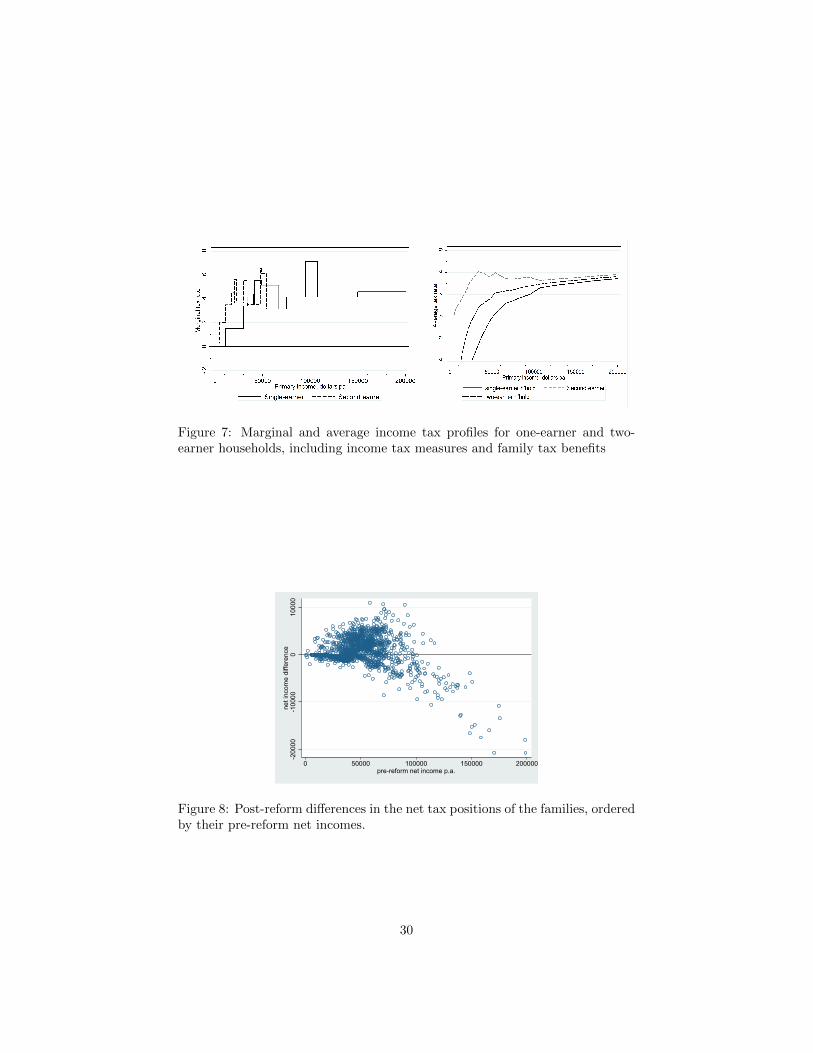
Figure 7 compares graphically the resulting profiles of marginal tax rateswith respect to primary income for a single-income family and for the secondearner in a two-income family in which both partners earn the same incomes.26
FTB payments are for two children under 13, with one under 5 years.
Figure 7 about here
The graph highlights two important effects of the Family Tax Benefit systemand ML. First, they raise marginal rates across bands of second income up to thefamily income threshold at which the payments are fully withdrawn. Secondly,they introduce a marginal rate scale with the highest rates applying acrossrelatively low and average incomes. For example, the marginal tax rate on amother’s earnings in a family with a primary earner on an average income canrise to over 70 cents in the dollar.
If we treat primary income as fixed and calculate the additional tax a familypays when the mother goes out to work, we obtain an average tax rate profilethat includes rates of over 40 per cent, as shown in Figure 7. Consistent withjoint taxation, average tax rates on the two-income family are much higher thanthe rates on the single-income family at any given level of primary income, untilthe payments are fully withdrawn. Under a tax system of this kind, the lowlevel of female hours reported in the preceding section is hardly surprising.
4.5.3 Childcare Benefit and Childcare Rebate
Childcare Benefit depends (among other things) on the ages of children, numberof children, type of childcare and the hours of childcare used. The benefit isphased out with rising family income according to the age of the child and thenumber of children receiving childcare.
23For a family with the youngest child aged 5 to 15 or full time student aged 16 to 18, thepayment is $2,595.15 per year.
24See Alesina, Ichino and Karabarbounis (2007).25Note that with selective taxation of this kind, partners in the two-income family no longer
face the same marginal tax rates.26Note that the marginal tax rate profile for the primary income earner in the two-income
household is the same as that shown for the second earner apart from higher rates at very lowlevels of second income due to FTB-B.
14
The Childcare Rebate reimburses families for their claimed childcare ex-penses. It can cover up to 50% of the net childcare expenses (that is, aftersubtracting CCB). The CCR rate is not income-tested, but it has an upper capon the amount of expenses which can be reimbursed. For the year 2008, thiscap was $4,354 per year.
5 Results
We first present the results for the baseline homogeneous specification presentedin subsection 3.1, and then discuss those for the extended model dealing withunobserved heterogeneity, as detailed in subsection 3.2.
5.1 Baseline Model: No Heterogeneity
The estimated parameters of the baseline model are reported in Table 2. Whilethe model does not control for unobserved heterogeneity, the computation timeis minimal. Moreover, if the homogeneity assumption were found to be valid,the results are consistent and more efficient than the latent class model. Thecoefficients indicate that several of the interaction terms yield intuitively plau-sible results. Increases in the number of pre-school aged children present in thehousehold raise the marginal utility of formal childcare, and therefore strengthenthe demand for it. On the other hand, increases in the (assumed exogenous)availability of informal childcare weaken it. The same is true for the time allo-cation to housework.
Table 2 about here
The estimated marginal utilities of the choice variables, the components ofthe vector µ, are central to our analysis, but their evaluation is more complexthan consideration of the simple regression coefficients in isolation, since theyinvolve the total effects of a change in one of these variables working throughthe entire matrix A and vector b. They are also household-specific, since theutilities Ψ(µ) depend on the household’s socio-demographic characteristics, X,as well as the values of its choice variables. Therefore we present the marginalutilities in two ways: first, by averaging them across the sample of households;and secondly, by presenting the proportion of households that are measured ashaving negative marginal utilities for each given choice variable. It is also usefulto identify separately the average marginal utility of each choice variable for thesubset of households which buy formal childcare. The results are presented inTable 3.
Table 3 about here
As we expect intuitively, marginal utilities of income, domestic childcareand housework/leisure are on average positive, with only very small fractions
15
of households having negative values at their computed optimal choice values.On the other hand, around 90% of households are reported as having negativemarginal utilities of formal childcare at their optimal choice levels. This isof course not a problem for those households which choose to consume zeroamounts of market childcare, but the last column of the table shows that thosehouseholds consuming positive amounts also on average have negative marginalutilities, which is clearly inconsistent with it having a positive price.
This counter-intuitive result can be potentially attributed to unobservedheterogeneity. An important observation in this respect is that our samplecontains a substantial share (57%) of households which do not use any formalchildcare. Such sample composition can prove problematic for the homogenousmodel, provided that the decision about formal childcare utilization is influencedby unobserved differences in mothers’ housework productivity. The model willtry to explain this relation in terms of the variables included in the utilityfunction, assigning strong disutility to formal childcare. Failure to account forunobserved heterogeneity will cause the coefficients of childcare to be biased,making it seemingly unattractive even for the active users. Therefore, it isindeed advisable to extend our analysis further and attempt to control for theunobserved heterogeneity in a flexible form.
5.2 Allowing for unobserved heterogeneity: the latent classmodel
A key step in the EM estimation procedure is the initial selection of the numberof latent classes. This decision involves a trade-off. On the one hand, the higherthe number of heterogeneous groups, the better will be the fit of the model,as we account for unobserved heterogeneity in a more flexible form. On theother hand, given that our sample is finite, more stratified models are bound toprove less efficient, as we estimate a new set of regression coefficients with eachadditional class. The determination of the number of classes is therefore crucialfor identifying the optimal model.
Following Train (2008), we compare the models with varying classificationchoices on the basis of their Schwarz-Bayesian information criteria (BIC)
BIC = −2 log(L) + k log(n) (12)
where L is the likelihood, k is the number of free parameters in the model andn is the number of observations in our sample. The multiple-class models yieldthe following statistics:
Table 4 about here
As we see, the 8-class model attains the lowest BIC, and should thereforebe considered as the most reliable specification for further analysis.
We do not present the regression coefficients for the 8-class model because theclass-level stratification makes their interpretation practically infeasible. The in-dicators of average marginal utilities suffer from the same problem due to the
16
logit normalization of each latent class. However, one statistic which remainsreadily interpretable is the share of the population with negative marginal util-ities.
Table 5 about here
The only share which exhibits a substantial change compared to the baselinespecification (cf. Table 3) is the one corresponding to formal childcare. Theshare of mothers exhibiting disutility from additional childcare drops by 30percentage points, attaining 53% in total, and 31% when we restrict ourselvesto the mothers who are actively using formal childcare.27 This is a considerableimprovement compared to the homogenous specification.
The relative performance of the models with varying numbers of latentclasses is further tested through a series of simulations in the next section. Theaim of these simulations is to predict how people respond to certain changeswithin their economic environment. By predicting (and comparing) the behav-ioral responses for different model specifications, we can draw inferences aboutthe importance of class-level heterogeneity, and assess the validity of the homo-geneity assumption.
6 Micro simulations
We evaluate the following changes: first, we simulate two basic adjustments tothe aggregate price level - a 10% increase in the net wages of mothers, and a10% increase in the net prices of formal childcare (Section 6.1). Second, wecarry out a policy simulation in the spirit of Apps & Rees (2009), building ontheir critique of FTB and other joint-income fiscal measures (as discussed inthe previous section). We propose an alternative system of taxes and benefitswhich aims to be less distortionary in respect of female labor supply than thecurrent one, and we estimate its impact on household choices within the sampleof households.
6.1 Changing net wages of mothers and net childcare prices
Increasing net wages results in higher disposable incomes for working mothers,and increasing net childcare prices has the opposite effect for families who areusing formally provided childcare. The analysis of net prices and wages is advan-tageous over the analysis of gross indicators, as it circumvents secondary incomeeffects caused by changes in the effective fiscal rules28. The resulting change indisposable incomes is hence equi-proportionate across households, which allowsus to isolate the direct effect of the proportional increase of wages and childcareprices.
27The latter is obtained by taking weighted means over all classes, where the weights arethe class probabilities given the observed choice.
28See Section 4.5
17
The impact of the pricing changes is measured in terms of aggregate elastic-ities. We compute the ratios of percentage changes in the relevant time use andcare variables to the percentage changes in the underlying policy instruments(wages and prices) which are 10 percent, by construction. Computation of theaggregate elasticities is carried out in the following way. We first derive thepre-reform time use allocations. This is done by averaging individual choiceprobabilities predicted by our logit model, and multiplying the results by thehours of time use activities corresponding to the given choice. This provides uswith a simulation of average time use hours, based on the estimated model.29
The computation of post-reform average hours is very similar to the pre-reform case. The only difference is that for the initial prediction of householdchoice probabilities we construct a new dataset with family incomes computedto be consistent with the specified reform. By feeding the augmented datasetinto our model, we can derive choice probabilities which would correspond tothe post-reform state of the world. The computation of average hours is thenthe same as above.
Having the pre-reform and post-reform allocations in hand, the last stepin the computation of the elasticities is a matter of straightforward arithmetic.The results for models with varying numbers of classes are provided in Table 6.30
Table 6 about here
When we allow for latent classes, the predicted responses to the wage in-creases in the policy reforms fall substantially, and remain relatively stableamong models with different number of classes. These results demonstrate theimportance of controlling for unobserved heterogeneity in our analysis.
Standard errors are on average rising as we allow for further classes, makingsome of the coefficients less significant for heavily stratified models. This reflectsthe fact that these models are more data-intensive. Nevertheless, in certaincases we observe that the standard errors fall as we move to the more stratifiedmodels. We attribute this effect to increased explanatory power of the latterspecifications.
Given the results of the BIC selection procedure discussed in the previoussection, the following discussion of simulation outcomes will focus on the optimalparameterization, that is, on the 8-class model.
In the case of the net wage increase, we observe time use shifts which corre-
29Ideally these simulated values should be close to their empirically observed counterparts.For the 8-class model, the simulated daily averages are 1.2 hours for formal childcare, 2.5hours for work, and 10 hours for housework. The corresponding observed mean values inthe data (after replacing each observed value by the mean of its category to account for thediscretization) are 1.2, 2.7 and 10.1, respectively.
30Standard errors on the elasticities were computed through 100 Monte Carlo simulations,re-computing the impact of the reforms with simulated sets of preference coefficients A andb. The coefficients were drawn through Cholesky decomposition of an underlying covariancematrix, which was derived using a ML procedure proposed by Ruud (1991), correcting forvariance of the aggregate class shares and covariance structure between different class-levelparameterizations.
18
spond to intuition. With the reform in place, a 10% wage increase results in a3.9% rise in average working hours, associated with a 2.7% increase in hours ofbought-in childcare.
The housework elasticity proves to be negative, at -0.06. The negative signimplies that higher wages lead the mothers to work less in the household. How-ever, the actual change of housework hours is not large enough to equilibratethe increase of working hours, which means that mothers give up both theirhousework and leisure activities in order to work more.
Turning to the impact of the rise in childcare prices, it is not surprisingthat the highest elasticity is that of formal care itself. With a 10% rise inchildcare prices, the demand for formal childcare falls by 6.9%. This in turncauses the mothers to work less in the market (hours drop by 1.4%), as theyhave to substitute their own time for bought-in services. Accordingly, the hoursof housework increase by 0.3%, replacing almost all of the forgone time formerlyspent on market work.
6.2 Policy simulation: alternative system of taxes andbenefits
As discussed earlier, the shift to joint taxation with the means testing of FTB-Aand the ML on family income can be expected to have substantial disincentiveeffects on female labor supply. We analyze this by simulating the effects ofswitching to an individual based income tax with universal payments.31 Weconstruct the reform by eliminating the ML and making the payments underFTB-A universal. A key feature of the reform is the removal of the excessivelyhigh effective marginal rates on the incomes of the majority of mothers underthe existing system.
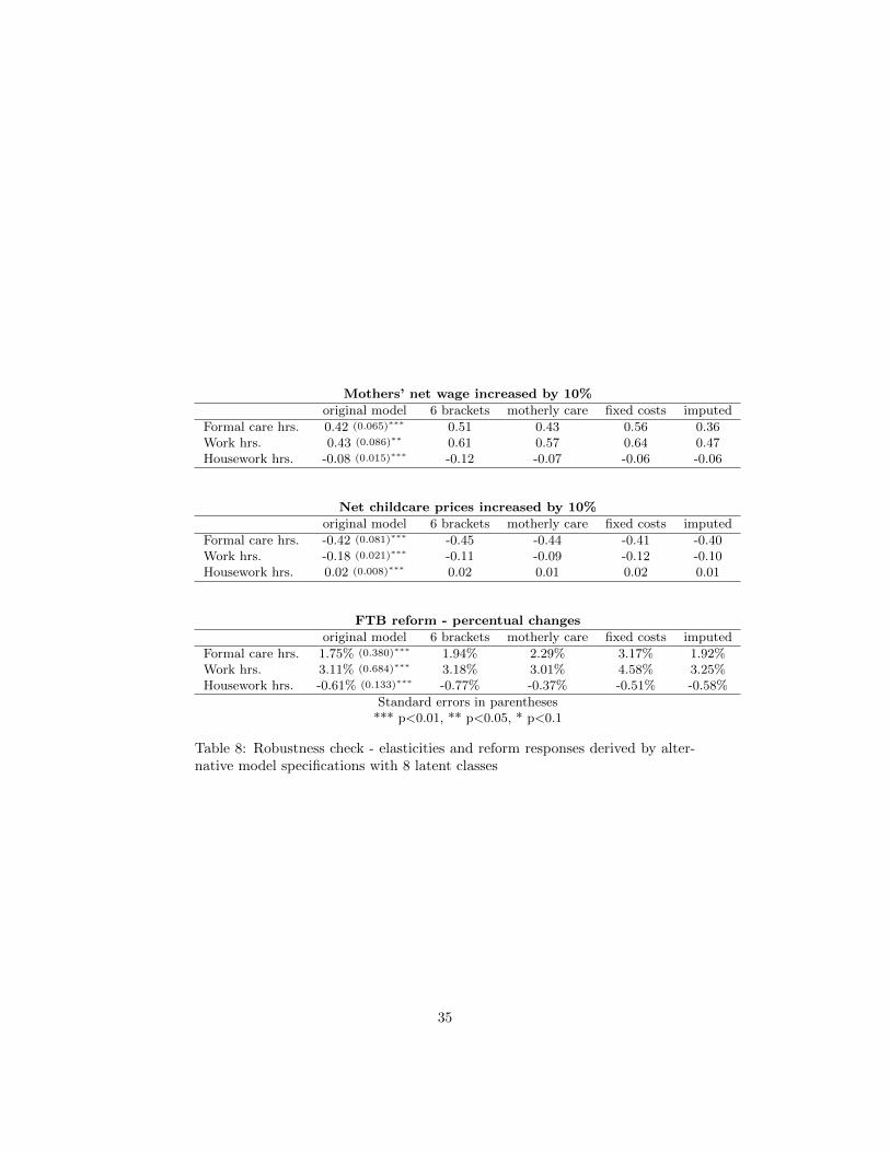
To fund the increase in benefit payments we introduce a proportional increasein the marginal tax rates of the PIT & LITO (see Section 4.5.1). Assuming nobehavioral responses, we calculate that an increase in tax rates of 26.76% wouldbe required for revenue neutrality.32 On the basis of this figure, we multiplyeach rate of the income tax by 1.2676, making the resulting personal income taxmore progressive than the original. Figure 8 presents the differences in the nettax positions of the households in our sample induced by the reform. The dif-ferentials are ordered by the corresponding pre-reform net household incomes,so that we can see how the tax burden shifts over different income groups.33
Figure 8 about here
31As proposed in Apps and Rees (2009).32The maintained assumption of no time allocation changes will inevitably be rejected by
our simulation results, but it serves as a useful reference point. When we predict the reform-induced changes in work and childcare hours, we are able to calculate the gains (or losses) intax revenue relative to the original setting due to these behavioral responses.
33Again, for the sake of presentation, we maintain the assumption that the individual timeallocations remain unchanged.
19
Looking at the scatter plot, we see that the increased progressivity of thepost-reform tax system shifts the tax burden towards the higher incomes, leavingmiddle-income families better off as compared to their original net tax positions.It is also interesting to note that the increased progressivity can be consideredto be a remedy for the forgone phasing-out of the family tax benefit, becausethe universal FTB payments will eventually be subtracted from the incomes ofhigh-earning households through the effect of increased income taxes.
Table 7 about here
As for the behavioral implications of our simulated policy change, Table 7presents changes in the time allocations induced by the reform. Similarly to theprevious simulations, we observe a large discrepancy between the sizes of thechanges predicted by the homogenous and latent-class models, with the results ofthe latent-class models proving relatively stable among different specifications.
Regarding the simulation outcomes, we again restrict ourselves to the 8-classspecification, in which we observe a 3.11% increase in the hours of work, a 1.75%increase of hours of formal care, and a 0.63% decrease in the hours of housework.
An interesting picture emerges when we compare responses to the FTB re-form on extensive and intensive margin of the labor supply. According to ourresults, the observed increase of aggregate working hours can be attributed bothto the newly employed mothers and to the mothers extending their original workallocation. This effect is stronger for mothers who report to work only in thehousehold, with the absolute increase of market work hours being 28% largerthan for those who are already in the labor force.
As for the change of formal childcare hours, the mothers in the householdexhibit rather modest increase in absolute terms (70% lower than the employedmothers), however in relative terms they raise their childcare allocation morethan employed women (the initial level of childcare utilization is substantiallylower for mothers in the household).
Naturally, this behavioral heterogeneity is crucial for successful targetingof the policy reform, as it helps us to identify its actual impacts on differentsubsamples of the population. But it is also interesting from the perspectiveof economic modelling, as we can compare the predicted outcomes of homoge-nous and latent-class models. When we run a similar analysis of behavioralresponses with the homogenous model specification, all the elasticities proveto be almost identical among both subgroups. Clearly, the homogenous modelfails to predict heterogenous responses on the extensive and intensive margin oflabor supply. This fallacy is further accented by the fact that the model cannotreplicate observed differences in reported time use allocations among the twogroups, overestimating work and formal childcare allocations of mothers in thehousehold, and underestimating them for the subsample of employed mothers.For these reasons, it is particularly hard to maintain that homogenous modelwould be able to provide practitioner with unbiased predictions of the responsesto proposed policy changes, as it cannot successfully replicate the behavior of
20
heterogenous groups present in the population sample.
We further analyze the net fiscal effect of the FTB reform, accounting forsubsequent changes in time allocations predicted by our 8-class model. Thesechanges play a major role in the context of reform evaluation, because they canturn the reform either more costly or more profitable than the original fiscalsystem34.
The key result in this context is that government breaks even and actuallyimproves its net fiscal position, although the nominal change is rather marginal.The income taxes of mothers rise by mere 0.5%, compared to the 3.1% increaseof aggregate working hours. Such difference in magnitudes relates to the factthat the FTB reform exerts highly heterogenous behavioral responses acrosshouseholds. Despite the aggregate increase of working hours among mothers, aconsiderable fraction (31%) actually reduce their work intensity, which lowersthe expected income tax proceeds. These mothers are mainly high-earners,who are already working and whose expected income falls after introducing thereform (due to the increase of income tax rates). Because of the progression ofthe income tax system, the fall of revenue from high earners offsets a large partof the new tax proceeds coming from low- and middle-income households, andpulls down the aggreagate revenue effect. More specifically, the expected averageincrement in annual income tax proceeds is 151$ for the mothers who raisetheir working hours (5.6% of their initial proceeds). For the rest of the sample,the tax proceeds decline by 261$ (2.3% of their initial proceeds), lowering theaggregate impact on income taxes to 25$ on average, which translates into theaforementioned 0.5% increase of mothers’ income taxes.
The situation is very similar for the childcare benefits, which also exhibit onlyslight increase of aggregate CCB & CCR payments as high-earning mothers optfor less formal child care35. The increase of annual CCB payments is rathersmall compared to the increase of tax proceeds, attaining on average 2$ (0.1%of the initial proceeds).
Adding the two fiscal effects together, we conclude that the households areexpected to raise their annual government contribution by 23$ on average. Thisrepresents 0.2% increase of their total income tax proceeds after subtractingall the family- and childcare-related benefits. However, despite having onlymarginal revenue effect on the side of government, the FTB reform is successfulin two other ways. It is able to increase employment among the population ofmothers with preschool children, and reduce the fiscal imbalances inherent inAustralian fiscal system. Furthermore, it should be emphasized that the size of
34Changes in time allocations can affect the government revenue through two distinct chan-nels: by raising the work intensity the mothers are also increasing their income tax proceeds,and by choosing longer childcare hours the families become eligible for more childcare benefits.
35This result hinges on the fact that the CCR benefits are calculated as a proportion of thetotal cost of childcare, allowing users of high-priced childcare to receive larger benefits. Witha system of benefits independent on claimed prices, the increase of childcare benefits wouldbe proportional to the elasticity of formal childcare hours, that is, 1.75%.
21
the reform effects is heavily dependent on the degree to which is the national taxsystem dependent on joint taxation. Running a similar policy simulation on datafrom countries with purely joint-income taxation would make the behavioralresponses considerably stronger.
6.3 Robustness checks
In order to assess stability of our results, we run a series of sensitivity checks,altering the econometric specification of our model in following ways:
To achieve more flexible specification, we divide the time use variables into afiner grid (63) of discrete choices, allowing for greater degree of discretion in thehousehold-level decision making. We also experiment with the composition oftime use variables, reducing the mother’s housework decision to a single choiceof motherly childcare36. Another pursued extension augments the model byfixed costs of working, being estimated as an additional parameter of the utilityfunction. Furthermore, to account for potential misreporting in the individualhousehold accounts, we estimate a model with all wages and childcare pricesimputed by our model.
Table 8 about here
The elasticities presented in Table 8 confirm that changes in the econometricspecification are likely to change nominal values of our results. Their relativesizes and signs remain however similar to the original model, with most of thevalues remaining in the 95% confidence interval of the corresponding baselineelasticities.
The stability of the elasticities is interesting in context of the model contain-ing motherly childcare decision, as it suggests that changes in the houseworkallocation are proportionate, irrespective of the distinction between childcare-related and other household activities. An engagement in the labor marketwill hence make the women work less in the household, delegating part of theirchores either to the husband, or buying in the services from the market.
Apart from direct changes of the model, we also evaluate the validity of stan-dard errors corresponding to the measured elasticities, controlling for generalheteroskedasticity and household-specific clustering. In both cases the newlyderived standard errors preserve significance levels attained by the standard ap-proach, suggesting that heteroskedasticity is not likely to distort our estimates.
36That way, we can examine direct substitution effects between informal and formal child-care. However, such adjustment comes at the cost of making the residual time allocation moredifficult to interpret, as it contains both leisure time and housework unrelated to childcare
22
7 Conclusions
In this paper we have analyzed the time allocation decisions of mothers withpre-school children with emphasis on their labor supply choices. We have fo-cused on the identification and analysis of unobserved heterogeneity, which hasits origins in across-household variations in productivity and preferences andwhich has proven to play a dominant role in the decision making of mothersin our data. The heterogeneity in unobserved productivities and tastes amongthe identified latent groups undermines the usefulness of the homogenous modelwith no unobserved heterogeneity. The parameters fail to capture the true ef-fects of factors driving household decision making, and hence simulations basedon the baseline homogeneous model specification can be expected to give mis-leading results.
To control for unobserved heterogeneity, we estimated a series of latent-classmultinomial logit models, taking the 8-class model to be the best parameteriza-tion. This model was found to perform optimally, balancing goodness of fit onthe one hand against parsimony on the other. To assess the responsiveness ofour sample to changes in the tax system and in childcare prices, we conducteda series of policy reform simulations, increasing net wages of mothers and netchildcare prices in the first two reforms, and altering the joint-income structureof the existing system in the third reform.
The first two micro simulations based upon our estimates show that mothersare responsive both to the changes in wages and childcare prices. This resultsuggests that market work and formal childcare tend to be complements, andrespond significantly to wage and price changes. The results also indicate thatsignificant changes in labor supply and childcare demand can remain uniden-tified when the unobserved heterogeneity is left untreated, thus significantlydistorting the size of predicted changes in female labor supply.
In the third simulation, we show that the tax measures that withdraw ben-efits on the basis of joint income are likely to prove adverse to the labor supplydecisions of working mothers, and that the tax system can be made more favor-able for employed mothers by switching to a fully individual based system. Insuch a setting, women are predicted to increase their labor supply and to utilizemore formal childcare. These responses also raise additional tax revenue whichcould be used to lower tax rates and therefore achieve efficiency gains.
A number of improvements and extensions are of course possible. First, ouranalysis would benefit from exploiting the panel structure of the HILDA dataset,controlling for time-stable individual effects. Secondly, although we consider thecurrent method of treating unobserved heterogeneity to perform well, it couldbe worthwhile to assess the stability of our results by using alternative ways ofcontrolling for unobserved heterogeneity, such as the random coefficient mixedlogit model, or the approaches utilizing Bayesian nonparametric methods.
23
References
[1] ALESINA, A., A. ICHINO & L. KARABARBOUNIS (2007): ”Genderbased taxation and the division of family chores”. Harvard University Dis-cussion Paper.
[2] APPS, P. & D. ALLEN (2012): TBA, forthcoming
[3] APPS, P. & R. REES (2009): Public Economics and the Household. Cam-bridge University Press
[4] BAKER, M., J. GRUBER & K. MILLIGAN (2008): Universal child care,maternal labor supply, and family well-being. Journal of Political Economy116(4): pp. 709–745
[5] BERNDT, E., B. HALL & R. HALL (1974): ”Estimation and inferencein nonlinear structural models”. In Annals of Economic and Social Mea-surement, Volume 3, number 4,” NBER, pp. 103-116. National Bureau ofEconomic Research, Inc
[6] BHAT, C. (2000): ”Flexible model structures for discrete choice analy-sis.” In Handbook of Transport Modeling, volume 1, pp. 71-90. Pergamon,Amsterdam, NL
[7] BLAU, D. (2003): Child care subsidy programs. In Means-Tested TransferPrograms in the United States, NBER Chapters, pp. 443–516. NationalBureau of Economic Research, Inc
[8] BLUNDELL, R. & A. SHEPHARD (2011): Employment, hours of workand the optimal taxation of low income families. IZA Discussion Papers5745, Institute for the Study of Labor (IZA)
[9] BURDA, M., M. HARDING & J. HAUSMAN (2008): ”A Bayesian mixedlogit & probit model for multinomial choice.” Journal of Econometrics147(2): pp. 232-246
[10] CAMERON, A. C. & P. K. TRIVEDI (2005): Microeconometrics. Cam-bridge University Press
[11] CONNELLY, R. (1992): ”The Effect of Child Care Costs on MarriedWomen’s Labor Force Participation.” The Review of Economics and Statis-tics 74(1): pp. 83-90
[12] CONNELLY, R. & J. KIMMEL (2003): Marital status and full-time/part-time work status in child care choices. Applied Economics 35(7): pp. 761–777
[13] DEMPSTER, A., N. LAIRD & D. RUBIN (1977): ”Maximum likelihoodfrom incomplete data via the EM algorithm.” Journal of the Royal Statis-tical Society. Series B 39(1): pp. 1-38
24
[14] DOIRON, D. & G. KALB (2005): Demands for child care and householdlabour supply in Australia. The Economic Record 81(254): pp. 215–236
[15] DUNCAN, A., G. PAULL & J. TAYLOR (2001): Mothers’ employmentand the use of childcare in the uk. IFS Working Papers W01/23, Institutefor Fiscal Studies
[16] HECKMAN, J. (1979): ”Sample selection bias as a specification error.”Econometrica 47(1): pp. 153-161
[17] HECKMAN, J. & B. SINGER (1984): ”A method for minimizing theimpact of distributional assumptions in econometric models for durationdata.” Econometrica 52(2): pp. 271-320
[18] KALENKOSKI, C. M., D. C. RIBAR & L. S. STRATTON (2005): Parentalchild care in single-parent, cohabiting, and married-couple families: Time-diary evidence from the united kingdom. American Economic Review 95(2):pp. 194–198
[19] KEANE, M. & R. MOFFITT (1998): ”A structural model of multiplewelfare program participation and labor supply.” International EconomicReview 39(3): pp. 553-589
[20] KIMMEL, J. & R. CONNELLY (2007): Mothers’ time choices: Caregiving,leisure, home production, and paid work. The Journal of Human Resources42(3): pp. pp. 643–681
[21] KORNSTAD, T. & T. THORENSEN (2007): A discrete choice model forlabor supply and childcare. Journal of Population Economics 20(4): pp.781–803
[22] PACIFICO, D. (2009): ”On the role of unobserved preference heterogeneityin discrete choice models of labor supply.” Working Paper Univ. Modena 1
[23] RIBAR, D. C. (1995): A structural model of child care and the labor supplyof married women. Journal of Labor Economics 13(3): pp. 558–97
[24] RUUD, P. (1991): ”Extensions of estimation methods using the EM algo-rithm.” Journal of Econometrics 49(3): pp. 305-341
[25] TRAIN, K. (2008): ”EM algorithms for nonparametric estimation of mix-ing distributions.” Journal of Choice Modelling 1(1): pp. 40-69
[26] TRAIN, K. (2009): Discrete Choice Methods with Simulation. CambridgeUniversity Press
[27] VAN SOEST, A. (1995): ”Structural models of family labor supply: Adiscrete choice approach.” Journal of Human Resources 30(1): pp. 63-88
[28] VAN SOEST, A. & E. STANCANELLI (2010): ”Does Income TaxationAffect Partners Household Chores ?” IZA Working Paper 1(5038)
25
[29] VAN SOEST, A., A., M. DAS & X. GONG (2002): A structural laboursupply model with flexible preferences. Journal of Econometrics 107(1-2):pp. 345–374
26
Figures and Tables
0.0
5.1
.15
.2D
ensity
0 50 100 150Weekly hours worked
menwomen
Figure 1: Distribution of weekly hours of market work in families with preschoolchildren
0.0
1.0
2.0
3D
ensity
0 50 100 150 200Weekly housework hours
menwomen
Figure 2: Distribution of weekly hours spent on housework in families withpreschool children
.
.
.
27
0.0
05
.01
.015
.02
.025
Density
50 100 150Weekly hours spent on leisure
menwomen
Figure 3: Distribution of weekly hours spent on leisure in families with preschoolchildren
0.0
1.0
2.0
3.0
4.0
5D
ensity
0 20 40 60 80 100Childcare hours
formalinformal
Figure 4: Distribution of weekly hours of informal and formal childcare, familieswith preschool children who are using childcare
28
05.0
e-0
61.0
e-0
51.5
e-0
52.0
e-0
52.5
e-0
5D
ensity
0 50000 100000 150000 200000Annual labor income
men women
05.0
e-0
51.0
e-0
41.5
e-0
4D
ensity
0 50000 100000 150000 200000Annual non-labor income
Figure 5: Distributions of labor and non-labor gross annual income, in Aus-tralian dollars, families with preschool children
Figure 6: Marginal and average income tax profiles, and annual income distri-butions for year 2008
29
Figure 7 Tax rates: 2007-08 PIT, LITO, ML and FTBs
Figure 7a Marginal tax rate
Figure 7b Average tax rates
2
Figure 7: Marginal and average income tax profiles for one-earner and two-earner households, including income tax measures and family tax benefits
-20000
-10000
010000
net in
com
e d
iffe
rence
0 50000 100000 150000 200000pre-reform net income p.a.
Figure 8: Post-reform differences in the net tax positions of the families, orderedby their pre-reform net incomes.
30
Table 1: Summary statistics, sample of couples with preschool childrenVariable Mean Std. Dev. Min. Max.
Age - women 32.9 5.6 16 48Age - men 34.9 6.3 18 58Marital status (dummy) 0.82 0.4 0 1Employment status - women (dummy) 0.55 0.5 0 1Employment status - men (dummy) 1 0 1 1
Number of children, aged 0-4 1.39 0.6 1 4Number of children, aged 5-9 0.47 0.7 0 4Number of children, total 2.01 0.96 1 6