Labor Taxation in Search Equilibrium with Home Production ¤ Bertil Holmlund Department of Economics, Uppsala University Box 513, SE-751 20 Uppsala, SWEDEN email: [email protected]This version: January 17, 2000 ¤ I thank Peter Fredriksson, Ann-So…e Kolm, Edmund Phelps and Peter Birch Sorenson for useful comments on an earlier draft. The paper was in part written during a stay at EPRU, University of Copenhagen.
Transcript
Labor Taxation in Search Equilibriumwith Home Production¤
Bertil HolmlundDepartment of Economics, Uppsala University
¤ I thank Peter Fredriksson, Ann-So…e Kolm, Edmund Phelps and Peter Birch
Sorenson for useful comments on an earlier draft. The paper was in part written
during a stay at EPRU, University of Copenhagen.
Abstract
Conventional models of equilibrium unemployment typically imply that pro-portional taxes on labor earnings are neutral with respect to unemploymentas long as the tax does not a¤ect the replacement rate provided by unem-ployment insurance, i.e., unemployment bene…ts relative to after-tax earn-ings. When home production is an option, the conventional results may nolonger hold. This paper uses a search equilibrium model with home pro-duction to examine the employment and welfare implications of labor taxes.The employment e¤ect of a rise in a proportional tax is found to be negativefor su¢ciently low replacement rates, whereas it is ambiguous for moderateand high replacement rates. Numerical calibrations of the model indicatethat employment generally falls when proportional labor taxes are raised.Progressive labor taxes increase labor market tightness but have ambiguouse¤ects on search e¤ort and employment. The numerical calibrations indicatepositive employment e¤ects.
JEL-codes: H24, J22, J64Keywords: Home production, job search, unemployment, taxation
1 Introduction
A popular theme in current policy discussions about labor market reformis that high taxes on labor contribute to high unemployment. Althoughthe claim appears intuitively plausible, it has not received overwhelmingsupport from theoretical and empirical research on unemployment and wagedetermination. In fact, proportional taxes on labor earnings are neutral withrespect to unemployment in many conventional models and the empiricalresearch has shown mixed results.1
Most of the theoretical models identify the ”bene…t regime” as the cru-cial factor that determines how labor taxes a¤ect labor costs and ultimatelyunemployment. Taxes are neutral as long as they do not a¤ect the after-taxreplacement rate, i.e., the relationship between income when unemployedand income when employed. There is in general complete real wage ‡exibil-ity with respect to changes in labor taxes if unemployment compensation isindexed to the real after-tax consumption wage through a …xed replacementrate. Labor taxes are then borne by labor and there is no e¤ect on laborcosts and unemployment.2
The potential for employment gains through lower labor taxes hinges onthe impact on the replacement rate; there will be an increase in employmentonly if the tax cut reduces the replacement rate. A bene…t regime involvingunemployment compensation …xed in real terms has this feature. A taxcut induces an increase in the real wage, which implies a decline in therelative compensation of unemployed workers. The tax cut works because ite¤ectively reduces the replacement rate.3
The existing literature on taxes and unemployment has paid little atten-tion to income sources other than labor earnings and unemployment ben-
1The large empirical literature involves numerous studies of the relationships betweenlabor costs and labor taxes. Tyrväinen (1995), Gruber (1997), Jackman et al (1996)and Nymoen and Rodseth (1999) are examples with somewhat con‡icting results. Otherstudies have investigated whether taxes help explain the evolution of unemployment overtime and di¤erences across countries; see for example Layard et al (1991), Elmeskov et al(1998), Nickell (1998), Madsen (1998), Phelps (1994) and Scarpetta (1996).
2This result holds in models with unions, as in Johnson and Layard (1986) or Layardet al (1991), as well as in models with bargaining between the …rm and the individualworker, as in Pissarides (1990). The result also holds in various e¢ciency wage models.
3Pissarides (1998) presents a number of simulation results that illustrate the quantita-tive importance of the bene…t regime for the e¤ects of changes in labor taxes.
1
e…ts.4 A shortcut is to allow for exogenous income or utility components,such as income from the ”informal sector”, income from home productionor a …xed value of leisure; see, for example, Bovenberg and van der Ploeg(1998) and Mortensen (1994). Tax cuts will bring about a fall in unemploy-ment provided that (i) the additional income sources are unresponsive tochanges in the real wage, and (ii) more prevalent among unemployed thanamong employed workers. The reason for this result is, again, that the taxcut reduces the e¤ective replacement rate by inducing a proportionally biggerincrease in labor income than in total unemployment compensation.
The purpose of this paper is to examine the e¤ects of labor taxes onlabor market outcomes in a model of equilibrium unemployment where theworker’s income from home production is endogenously determined. To thisend a search equilibrium framework along the lines of Pissarides (1990) isextended to allow for home production.5 Time devoted to home productionis taken to be a choice variable for both employed and unemployed individu-als: the employed worker chooses between time in market work and time inhome production, whereas the unemployed worker allocates his time betweenjob search and home production. The e¤ective replacement rate – inclusiveof income from home production – is endogenous in this environment, irre-spective of whether unemployment bene…ts are indexed to labor earnings or…xed in real terms.
For simplicity, we focus on a one-sector economy where the good pro-duced in the household is a perfect substitute to the market produced good.The model is thus not designed to shed light on the e¤ects of sectoral taxdi¤erentiation, where the di¤erentiation may depend on the degree of substi-tutability between market and nonmarket goods. The existing literature ontaxation and household production has been primarily concerned with thecase for tax di¤erentiation. The contributions in this …eld include papers bySandmo (1990), Fredriksen et al (1995), Sorensen (1997), Kolm (1998) andJacobsen Kleven et al (1999). Sandmo and Jacobsen Kleven et al considereconomies with competitive labor markets, whereas the other three papersallow for unemployment due to real wage rigidities.
4A remarkable exception is Edmund Phelps, who in a series of contributions has em-phasized the role of wealth and nonwage income in the theory of unemployment. See,for example, Phelps (1994), Phelps and Zoega (1998), and Hoon and Pelps (1996, 1997).These models imply neutrality of the labor tax in the long run, i.e., once wealth hasadjusted.
5The seminal paper on the microeconomics of home production is Gronau (1977).
2
Kolm’s model is richer than ours in some dimensions and more restrictivein others. Her model features two market sectors, with one of them producinggoods that are perfect substitutes to the goods produced at home. Jobsearch is ignored, however, which implies that the opportunity cost of homeproduction is zero for the unemployed worker. A corner solution is thenobtained where the unemployed worker allocates all available time to homeproduction. Another di¤erence is that Kolm’s analysis is based on a staticmodel with no attention paid to future transitions across labor market states.Such intertemporal aspects are crucial in the present paper and deliver a linkbetween bargained wages and general labor market conditions.
One might ask whether the incorporation of home production in thesearch equilibrium model is equivalent to accounting for (endogenous) leisure,as in Pissarides (1990, ch 6), Hansen (1998) or Marimon and Zilibotti (1999).In some sense, models of home production are observationally equivalent tomodels without, since ”for any model with home production, there is a modelwithout home production, but with di¤erent preferences, that generate thesame outcome for market quantities” (Benhabib et al, (1991), p 1170). Alongthis line of argument, one might argue that any result can be produced bysu¢cient imagination regarding the speci…cation of preferences. Indeed, thetax-neutrality results obtained in many standard models hinge on speci…cassumptions regarding preferences, typically utility functions that are iso-elastic in income.
By introducing home production in the present analysis we can build amodel that encompasses two predictions that appear empirically relevant:(i) hours of work are decreasing in the labor tax rate, and (ii) equilibriumunemployment is independent of the level of productivity. The second ofthose predictions can also be generated by a model with endogenous leisure,provided that the utility function is of the Cobb Douglas variety; see Fredriks-son and Holmlund (1998). The Cobb Douglas representation of preferencesis restrictive for the purposes of this paper, however, as it implies that hoursworked do not respond to after-tax wages.
The next section of the paper presents the basic model, where it is as-sumed that work-hours are determined by the individual employed worker.Section 3 turns to the e¤ects of changes in labor taxes in the basic model.The main analytical result is that a rise in a proportional tax reduces equi-librium employment as long as the replacement rate is zero or close to zero.We also consider progressive taxes and show that an increase in progressivityraises labor market tightness, whereas the e¤ect on employment is generally
3
ambiguous. Numerical simulations of the model indicate positive e¤ects onemployment.
Section 4 anlyzes the e¤ects of tax policies under the assumtion that thereis bargaining over work-hours between the worker and the …rm. The resultsare broadly similar to those obtained when work-hours are at the worker’sdiscretion.
2 The Model
2.1 The Labor MarketThe number of individuals in the economy is …xed and normalized to unity.The individuals are either employed or unemployed, the time horizon is in…-nite and time is continuous. Employed workers are separated from their jobsat the exogenous rate Á. Unemployed workers …nd new jobs at a rate thatdepends on their search e¤ort, s, as well as general labor market conditions.If u denotes the number of unemployed workers we can take su to representthe e¤ective number of job searchers in the economy.
The matching process is given by a standard concave and constant-returns-to-scale function that relates the ‡ow of hires, H, to the number of vacancies,v, and the e¤ective number of job searchers, su, i.e., H(v; su). The rate atwhich the unemployed worker …nds a new job is given by sH(v; su)=su =s®(µ), where µ = v=su is a measure of labor market tightness and ®(µ) =H(v; su)=su = H(µ; 1). The rate at which …rms …ll vacancies is given asq(µ) = H(v; su)=v = H(1; 1=µ). Hence, ®(µ) = µq(µ), where ®0(µ) > 0 andq0(µ) < 0; the tighter the labor market, the easier for workers to …nd jobsand the more di¢cult for …rms to …nd workers. Moreover, note that the elas-ticity of the expected duration of a vacancy with respect to tightness fallsin the unit interval, an implication of constant returns to matching; we have´ ´ ¡µq0(µ)=q(µ), where ´ 2 (0; 1).
The ‡ow equilibrium for the economy can be written as an unemploymentequation of the form:
u =Á
Á+ s®(µ)(1)
4
2.2 Worker Behavior
Individuals are risk neutral, face an exogenous interest rate, r, and deriveutility from consumption of the single good in the economy. The good iseither purchased from the market or produced at home. Assume that thedecision over hours of work is taken by the employed worker, who allocates theavailable time, normalized to unity, to market work, l, and home production,i.e., 1 = l + he. The unemployed worker divides his time between search,s, and home production, i.e., 1 = s + hu. The home production function,zj = z(hj), j = e; u, is increasing and strictly concave.
The employed worker’s instantaneous income is given as Ie = wl+z(he)+R, where w is the real hourly wage and R is a lump sum transfer fromthe government. The unemployed individual’s income derives from homeproduction, the transfer and unemployment bene…ts (Zb), i.e., Iu = z(hu) +R+ Zb.
Let U and E denote the expected present values of being unemployedand employed, respectively. The value functions for worker i can be writtenas follows:
rEi = wili + z(hei ) +R+ Á(U ¡Ei) (2)rUi = z (hui ) +R+ Zb + si®(µ) (E ¡ Ui) (3)
In a symmetric equilibrium, the utility di¤erence between the expectedpresent values is independent of the transfer and given as:
E ¡ U =Ie ¡ Iu
r + Á+ s® (µ)(4)
The employed worker allocates his time so as to maximize rEi, which isequivalent to maximization of the instantaneous utility. Assuming an interiorsolution, this yields the familiar ”pro…t maximization” condition:
z0(hei ) = wi (5)
implying that the marginal productivity of home production equals the realwage. Since the production function is strictly concave, it follows imme-diately that a rise in the wage causes a reduction in time spent in home
5
production and an increase in time spent in market work: @hei=@wi < 0 and@li=@wi > 0. The indirect utility function is given as Ie(wi). Note also thatthe e¤ect of a wage increase on the indirect utility is given as @Iei =@wi = li,by the envelope theorem.
The unemployed worker chooses search intensity, si, to maximize rUi.The …rst-order condition for an interior solution takes the form:
z0(hui ) = ®(µ)(E ¡ Ui) (6)
The left-hand side is the marginal cost of increasing search, which isforegone home production. The right-hand side is the expected marginalreturn from an increase in search e¤ort.
By making use of (4) and (6) we obtain the partial equilibrium results thatan increase in the market wage as well as an increase in labor market tightnessreduces time in home production (and thus increases search): @hui =@w < 0and @hui =@µ < 0. These results are implied by the concavity of the productionfunction and the fact that E ¡ U is increasing in the wage as well as intightness; note that the right-hand side of (6) is independent of search e¤ort(time spent in home production), by the envelope theorem. A rise in thewage increases the utility surplus from employment, which encourages search(discourages home production). A rise in tightness increases the marginalreturn from search, which has similar e¤ects. Also notice that E ¡ U isdecreasing in the bene…t level, which in turn discourages search e¤ort; hence@hui =@Zb > 0.
2.3 Firm Behavior
The model of the …rm follows Pissarides (1990) with explicit allowance madefor hours of work. Let V be the value of an un…lled job and J denote thevalue of a …lled job. The value functions are:
Labor productivity – output per hour – is constant and denoted y. Thecost of holding a vacancy is ky, with k > 0.6 t is a proportional payroll taxrate. Invoking the standard free entry condition for vacancies, V = 0, wecan derive
J =kyq(µ)
=yl ¡ w(1 + t)lr + Á
(9)
which implies a relationship between the hourly wage cost, wc ´ w(1 + t),and labor market tightness, conditional on hours of work:
wc = yµ1 ¡ (r + Á)kq(µ)l(w)
¶(10)
A rise in working time increases the ”feasible” real wage, given tightnessand the tax rate. One can think of this as follows. The …rm has a produc-tion department and a personnel department. A rise in work-hours allowsthe …rm to transfer some workers from recruitment activities to productionwhile keeping its total workforce constant. The higher output per employedworker implies a higher feasible real wage. We refer to this mechanism as theproductivity e¤ect of longer work-hours.
The slope of the labor demand relationship in (10) in the (wc,µ)-space isgiven as
sign@wc@µ
= signf¡1 + "S(ywc
¡ 1)g (11)
where "S ´ wl0(w)=l(w) > 0 is the wage elasticity of labor supply and y=wc >1, as given by (10).
Empirical estimates of the labor supply elasticity typically falls in a rangefrom zero to unity.7 If "S = 1, the ratio y=wc must exceed two in order toobtain a positive sign. This possibility is rather remote, however, as it wouldrequire unrealistically high vacancy costs. We thus assume @wc=@µ < 0.
6The appendix gives a rationalization for this speci…cation of vacancy costs, using amodel of a large …rm that allocates its workforce between production and recruitmentactivities.
7The recent and comprehensive survey by Blundell and MaCurdy (1999) reports esti-mates centered around 0.10 for males and around 0.7 for females.
7
Since w = wc=(1 + t) we can use (10) and express the worker’s real wageas a function of tightness and the tax rate: w = !(µ; t), with !µ < 0 and!t < 0. The higher the tax rate, the lower the feasible wage at a given levelof labor market tightness.
For later use we derive an expression for the ”µ-constant” wage elasticitywith respect to a tax increase:
»wt ´ ¡µ@ lnw@ ln(1 + t)
¶
¹µ=
11 ¡ "S [(y=wc) ¡ 1]
(12)
where »wt > 1. Note that »wt is increasing in the labor supply elasticity. Ahigher tax rate reduces the feasible real wage directly as well as indirectlythrough the induced decline in work-hours and the associated negative pro-ductivity e¤ect. The more sensitive work-hours are with respect to a declinein the wage, the sharper the reduction in hours and the stronger the negativeimpact om the feasible wage.
It is convenient to combine the expression for the worker’s utility surplus,E¡U , as given by (4), with the labor demand relationship in (10). We referto this expression as the ”feasible utility surplus”, denoted by F (¢):
E ¡ U = F (µ; t) ´ Ie(!(µ; t)) ¡ Iu(hu; Zb)r + Á+ s® (µ)
(13)
The right-hand side of (13) is independent of hu (and s), by the envelope the-orem; the unemployed worker’s maximization of the value of unemploymentis equivalent to minimization of the utility di¤erence E ¡ U . Moreover, theworker’s surplus is increasing in the wage and decreasing in tightness. Byinvoking the labor demand relationship we can by straightforward di¤eren-tiation establish that Fµ < 0 holds.
2.4 Wage DeterminationWages are determined in decentralized Nash-bargains between individual…rms and workers, recognizing that working time is optimally determinedby employed workers once the wage is set. The employed worker’s indirectutility function is given as Ie(wi), with the partial derivative @Iei =@wi = li .The Nash bargain thus solves:
8
maxwi
(wi; l(wi)) = [Ei(wi) ¡ U ]¯ [Ji(wi) ¡ V ]1¡¯
The …rst-order condition for this problem can be written as
E ¡ U =µ¯
1 ¡ ¯
¶µ1
1 + t
¶J (14)
where the free entry condition V = 0 is imposed. J = ky=q(µ) is impliedby these assumptions. One can think of (14) as yielding a ”bargained realwage”, conditional on labor market tightness and the tax rate. Alternatively,we can regard (14) as an equation that determines the ”bargained surplus”,B(µ; t), conditional on labor market tightness and the tax rate:
E ¡ U = B(µ; t) ´µ¯
1 ¡ ¯
¶µ1
1 + t
¶kyq(µ)
(15)
It is clear that Bµ > 0 holds since q0(µ) < 0. Note also that Bµµ < 0always holds for a matching function where ´ ´ ¡µq0(µ)=q(µ) is constant.We assume B(µ; t) = 0 for µ = 0. The Nash bargain delivers a worker surplusthat is proportional to the value of a …lled job, which in equilibrium mustequal the expected vacancy cost. A rise in labor market tightness impliesthat the expected duration of a vacancy, 1=q(µ), increases, which in turnmeans that the value of a …lled job rises. The Nash bargain gives workers ashare of the rise in total match surplus; hence the rise in bargained workersurplus.
2.5 EquilibriumIt will be convenient to characterize the equilibrium of the model by makinguse of two relationships, namely the feasible surplus, F (µ; t), and the bar-gained surplus, B(µ; t), as illustrated in Figure 1. Since Fµ < 0 and Bµ > 0,the equilibrium is unique and labor market tightness is given as the solutionto the equation ª ´ F (µ; t) ¡B(µ; t) = 0, i.e.,
ª ´ Ie(!(µ; t)) ¡ Iu(hu; Zb)r + Á+ s® (µ)
¡µ¯
1 ¡ ¯
¶µ1
1 + t
¶kyq(µ)
= 0 (16)
9
BF
θ
E-U
Figure 1: Labor Market Equilibrium
Many of the comparative statics properties of the model are conventional,at least as far as the e¤ects on tightness are concerned. The e¤ect on tightnessfollows by implicit di¤erentiation of (16), noting that ªµ < 0; the sign of thee¤ect of, say, a rise in the interest rate is thus given by the sign of ªr. Itis clear that labor market tightness falls as a response to: (i) a rise in theworker’s bargaining power, ¯; (ii) a rise in the cost of holding a vacancy, k;(iii) a rise in the discount rate, r; (iv) a rise in the separation rate, Á; and(v) a rise in the bene…t level, Zb.
The response to changes in labor productivity is somewhat less obvious.We wish to have a model with the realistic – and therefore attractive –property that labor market tightess and unemployment are independent ofthe level of productivity. Two additional assumptions are introduced toachieve this:
(i) Unemployment bene…ts are indexed to labor earnings through a …xedreplacement rate, i.e., Zb = ½wl .
(ii) The home production functions are given as zj = ayf(hj), where a isa positive constant and j = e; u. In words: productivity in home productionrises along with productivity in market production.
With these assumptions we can state the following result:
10
Lemma 1: A uniform increase in labor productivity, i.e., an increase in y,is neutral with respect to labor market tightness, hours of work in the marketand in the household, search e¤ort, and unemployment: dµ=dy = dhe=dy =dl=dy = dhu=dy = ds=dy = du=dy = 0:
To prove Lemma 1, note that optimal time allocation for the employedworker implies a relationship of the form he = h(w=ay) and thus also l =l(w=ay). The labor demand condition implies a relationship of the formw=y = Ã(µ; l(w=ay)) ¢ (1 + t)¡1, which can be written as w=y = x(µ; t). Sub-stituting into (16) while recognizing that zj = ayf(hj) and Zb = ½w (¢) l (¢)yield an expression from which y can be eliminated. µ is thus independent ofy. Also, using (1), it is clear that unemployment is independent of the levelof productivity.8
3 The E¤ects of Taxes
We proceed to investigate the e¤ects of labor taxes, assuming that tax rev-enues are spent as uniform lump sum grants to each individual in the econ-omy. The utility di¤erence between employed and unemployed workers isthus not a¤ected by the amount of tax revenues raised. The revenue sideof the tax system is hence neutral with respect to the real outcomes in theeconomy and we can examine the e¤ects of varying the tax rates withouthaving to consider how the tax revenues are used. The government’s bud-get restriction, given as t(1 ¡ u)wl = R + u½wl, is always ful…lled throughadjustment of the lump sum grant.
3.1 Proportional Taxes
From inspection of (16), it is clear that the payroll tax rate, t, a¤ects tightnessthrough several routes. First, a tax increase a¤ects the feasible surplus tothe worker by reducing the real wage and thereby the worker’s utility fromemployment: Ie(w) = Ie(!(µ; t)), with !t < 0. The F (¢)-schedule is shiftedto the left. This e¤ect tends to reduce tightness. A second e¤ect operates
8The conditions for ªµ < 0 are more restrictive when the bene…t level depends onearnings. See the Appendix.
11
through the bene…t level when bene…ts are indexed to earnings. The higherthe tax rate, the lower the bene…t level and the higher the feasible surplusto the worker. A third e¤ect works through the bargained surplus, whichis reduced by a higher tax; the B(¢)-schedule is shifted to the right. Thise¤ect is driven by the fact that a higher marginal payroll tax rate increasesthe cost to the …rm of raising the wage, which in turn tends to induce wagemoderation; E ¡ U thus falls, given tightness.
These e¤ects work partly in opposite directions. It is instructive to beginwith a special case where the replacement rate is zero, in which case theinduced e¤ect on bene…ts does not appear.
A Special Case: ½ = 0To obtain the net e¤ect we di¤erentiate (16) implicitly and obtain:
sign ªt = sign fze ¡ zu + (1 ¡ »wt )wlg (17)
where »wt > 1 as stated in (12).9 To sign ªt we need to determine the sign ofthe term ze ¡ zu. In other words, how does time in home production di¤erbetween employed and unemployed workers? We can state the followingresults:
Lemma 2: The allocation of time in equilibrium involves he < hu and hencel > s and ze < zu, provided that the production functions are of the formzj = ayf(hj), j = e; u.
Note that the equality he = hu would require equality between themarginal return to market work and the marginal return to search, i.e.,w = ® (E ¡ U). However, it can be shown that the inequality w > ® (E ¡ U)holds, implying that unemployed workers spend more time in home produc-tion than those who are employed. The proof is given in the Appendix.
Also note that the elasticity »wt is present in (17). The adverse e¤ect ontightness is reinforced by a large value of »wt . From (12) we have that »wt isincreasing in the labor supply elasticity, "S. A reasonable conjecture, then,is that the magnitude of the response of tightness to a tax hike is increasingin the supply elasticity. The reason is that a rise in the tax rate reducesthe worker’s indirect utility from employment as given by @Ie(w)=@t =
9In a model without home production and with exogenous work-hours, the oppositee¤ects on F (¢) and B(¢) would be exactly o¤setting. Note that »w
t = 1 is implied byexogenous work-hours. This fact, together with ze = zu = 0, imply ªt = 0.
12
l (@w=@t). Using (12) we obtain @Ie(w)=@t = ¡wl»wt =(1 + t). The induceddecline in the real wage is stronger, the higher the supply elasticity is. Theexplanation is that the decline in work-hours is stronger, which in turn re-inforces the fall in the feasible real wage (through the adverse productivitye¤ect).
Lemma 2 in conjunction with (17) thus imply dµ=dt < 0; a tax increasereduces labor market tightness. To obtain the e¤ect on unemployment weneed to consider how search e¤ort is a¤ected. Use the …rst-order conditionfor optimal search in (6) together with the Nash rule in (14) and the factthat J = ky=q(µ) to obtain:
z0(hu) = µ(t)µ¯
1 ¡ ¯
¶µky
1 + t
¶(18)
The right-hand side of (18) is the equilibrium marginal return to search,or the shadow wage of home production for an unemployed worker. A taxhike thus increases home production – reduces search – both directly andindirectly through µ(t). The e¤ect on unemployment is obtained by di¤er-entiation of eq. (1), recognizing ® = ®(µ(t)) and s = s(µ(t); t). The result isdu=dt > 0.
A tax increase produces an unambiguous decline in the real wage. Usew = !(µ(t); t) and di¤erentiate to obtain dw=dt < 0 (see Appendix). Thee¤ects on he(w(t)) and l(w(t)) are thus positive and negative, respectively.
We summarize the results for the special case as follows:
Proposition 1: A tax increase has the following e¤ects on labor market tight-ness, real wages, home production, work-hours, search and unemployment :dµ=dt < 0, dw=dt < 0, dhe=dt > 0, dhu=dt > 0; dl=dt < 0, ds=dt < 0, anddu=dt > 0.
The General Case: ½ ¸ 0Tax changes will in general induce changes in the bene…t level, which in turnin‡uence the overall e¤ects of taxes. The equation for equilibrium tightnesstakes the form:
ª¤ ´ Ie(w) ¡ Iu(hu; ½wl)r + Á+ s® (µ)
¡µ¯
1 ¡ ¯
¶µ1
1 + t
¶kyq(µ)
= 0 (19)
13
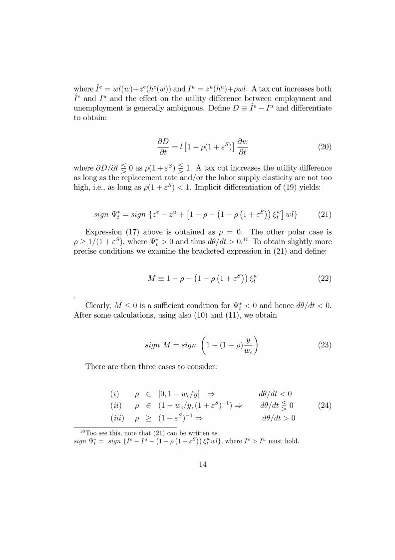
where Ie = wl(w)+ze(he(w)) and Iu = zu(hu)+½wl. A tax cut increases bothIe and Iu and the e¤ect on the utility di¤erence between employment andunemployment is generally ambiguous. De…ne D ´ Ie ¡ Iu and di¤erentiateto obtain:
@D@t
= l£1 ¡ ½(1 + "S)
¤ @w@t
(20)
where @D=@t Q 0 as ½(1 + "S) Q 1. A tax cut increases the utility di¤erenceas long as the replacement rate and/or the labor supply elasticity are not toohigh, i.e., as long as ½(1 + "S) < 1. Implicit di¤erentiation of (19) yields:
sign ª¤t = sign fze ¡ zu +
£1 ¡ ½¡
¡1 ¡ ½
¡1 + "S
¢¢»wt
¤wlg (21)
Expression (17) above is obtained as ½ = 0. The other polar case is½ ¸ 1=(1 + "S), where ª¤
t > 0 and thus dµ=dt > 0.10 To obtain slightly moreprecise conditions we examine the bracketed expression in (21) and de…ne:
M ´ 1 ¡ ½¡¡1 ¡ ½
¡1 + "S
¢¢»wt (22)
.Clearly, M · 0 is a su¢cient condition for ª¤
t < 0 and hence dµ=dt < 0.After some calculations, using also (10) and (11), we obtain
(iii) ½ ¸ (1 + "S)¡1 ) dµ=dt > 010Too see this, note that (21) can be written as
sign ª¤t = sign fIe ¡ Iu ¡
¡1 ¡ ½
¡1 + "S
¢¢»w
t wlg, where Ie > Iu must hold.
14
The condition for an unambiguously negative e¤ect is strong, since theinequality ½ · 1¡wc=y is easily violated for reasonable values of hiring costs.For example, the parameters used in our subsequent calibrations result invalues of wc=y exceeding 0:9, which implies that the replacement rate wouldhave to be lower than 0:1 to get an unambiguously negative e¤ect. Note,however, that the condition is su¢cient but not necessary for dµ=dt < 0.
A tax increase may have a substantial negative e¤ect on the bene…t levelif the replacement rate is high and supply very elastic (so that the earningsresponse is substantial). This implies that labor market tightness may in-crease when taxes are raised. The e¤ect on employment is ambiguous ingeneral, but negative for the …rst case in (24); the decline in tightness in-duces a decline in search e¤ort and employment falls. Note that an increasein tightness need not imply a rise in employment since search e¤ort maydecline.
There are limits to how high a replacement rate the model can take.The e¤ective replacement rate, Iu=Ie, must be lower than unity to inducemarket participation. The statutory replacement rate, ½, must be lower thanthe e¤ective rate since home production during unemployment exceeds homeproduction during employment. Formally, the inequality Iu < Ie requires½ < 1 ¡ (zu ¡ ze) =wl.
3.1.1 Calibration
We proceed to a numerical calibration of the model. The matching functionis taken to be Cobb Douglas, i.e., H = m(su)´(v)1¡´; it is straightforward toshow that this implies ¡µq0(µ)=q(µ) = ´. We also assume that the worker’sshare of the total match surplus equals the elasticity of matching with re-spect to unemployment, i.e., ¯ = ´; this is the so called Hosios-conditionthat implies that the search equilibrium outcome is e¢cient under certainconditions (Hosios, 1990). We set ¯ = ´ = 0:5.
The home production functions are of the form:
zj = ay¡hj
¢b (25)
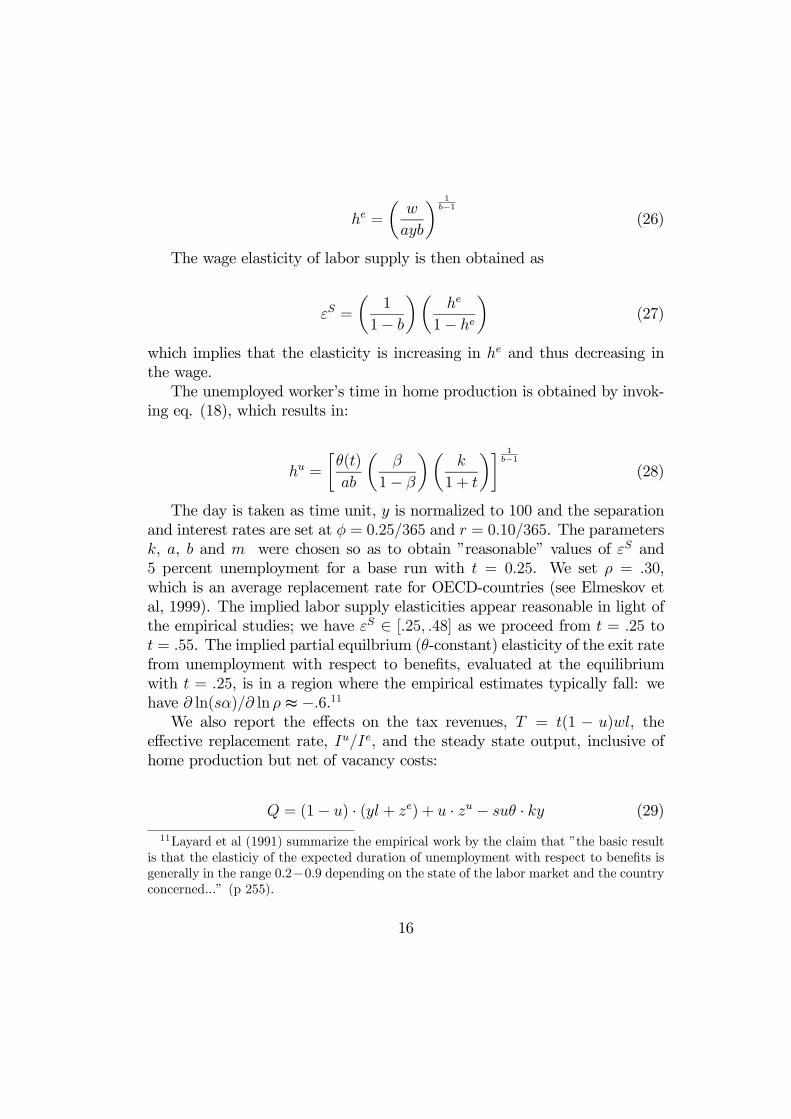
for j = e; u and b < 1. Optimal time allocation for the employed worker isthus given as
15
he =µwayb
¶ 1b¡1
(26)
The wage elasticity of labor supply is then obtained as
"S =µ
11 ¡ b
¶µhe
1 ¡ he¶
(27)
which implies that the elasticity is increasing in he and thus decreasing inthe wage.
The unemployed worker’s time in home production is obtained by invok-ing eq. (18), which results in:
hu =·µ(t)ab
µ¯
1 ¡ ¯
¶µk
1 + t
¶¸ 1b¡1
(28)
The day is taken as time unit, y is normalized to 100 and the separationand interest rates are set at Á = 0:25=365 and r = 0:10=365. The parametersk, a, b and m were chosen so as to obtain ”reasonable” values of "S and5 percent unemployment for a base run with t = 0:25. We set ½ = :30,which is an average replacement rate for OECD-countries (see Elmeskov etal, 1999). The implied labor supply elasticities appear reasonable in light ofthe empirical studies; we have "S 2 [:25; :48] as we proceed from t = :25 tot = :55. The implied partial equilbrium (µ-constant) elasticity of the exit ratefrom unemployment with respect to bene…ts, evaluated at the equilibriumwith t = :25, is in a region where the empirical estimates typically fall: wehave @ ln(s®)=@ ln ½ t ¡:6.11
We also report the e¤ects on the tax revenues, T = t(1 ¡ u)wl, thee¤ective replacement rate, Iu=Ie, and the steady state output, inclusive ofhome production but net of vacancy costs:
Q = (1 ¡ u) ¢ (yl + ze) + u ¢ zu ¡ suµ ¢ ky (29)
11Layard et al (1991) summarize the empirical work by the claim that ”the basic resultis that the elasticiy of the expected duration of unemployment with respect to bene…ts isgenerally in the range 0:2¡0:9 depending on the state of the labor market and the countryconcerned...” (p 255).
16
A measure of the marginal social cost of raising taxes – or marginal ex-cess burden – is given by ¢Q=¢T , the change in total output per dollar ofadditional tax revenues.
Table 1 shows the results of the calibrations. Tax increases produce mod-est increases in unemployment at low initial tax rates and more substantiale¤ects at high rates. A comparison with the estimates reported in the recentstudy by Elmeskov et al (1998) is useful. This study, based on pooled datafor 19 OECD countries for the period 1983-95, suggests that a rise in theoverall tax rate by 10 percentage points would raise the unemployment rateby slightly more than one percentage point. These results are broadly in linewith the simulation results in Table 1.
The e¤ective replacement rate increases from 55 to 78 percent as taxrates are increased from 25 to 55 percent. There are no La¤er-e¤ects, i.e.,higher tax rates do produce higher tax revenues. The marginal excess bur-den is modest for low tax rates but substantial for high rates. We have¢Q=¢T = ¡:18 for tax increases from 25 to 35 percent and ¢Q=¢T = ¡1:06for increases from 45 to 55 percent
Table 1. The E¤ects of Tax Increases (Proportional Taxes)
Parameters: ¯ = ´ = :5, y = 100, k = :676, a = :5, b = :6,m = :01939, r = :10=365, Á = :25=365, ½ = :3
t = :25 t = :35 t = :45 t = :55µ :904 :889 :866 :829
3.2 Progressive TaxesIt is well known that progressive taxes are conducive to wage moderation ina variety of non-competitive models of wage determination.12 Wage moder-ation is also associated with higher employment in the standard bargaining(or e¢ciency wage) models. We examine whether these results carry overto a search equilibrium model with home production and endogenous searche¤ort. There is no general presumption that the results will carry over, thereason being that the e¤ect on wage setting is not su¢cient to determine thee¤ect on employment.
The tax function facing the single …rm is taken to be linear and of theform:
¡i = ¹0 + ¿wi (30)
The marginal payroll tax rate is denoted ¿ and the intercept, ¹0, capturesthe non-proportionality of the tax system; ¹0 < 0 – a tax allowance – impliesa progressive tax schedule. The tax allowance is taken as given by each …rmand worker. We will, however, assume that it is indexed ex post to the generalwage level, i.e., ¹0 = ¹w. The hourly wage cost facing a representative …rm inequilibrium is thus given as wc = (1+¹+¿)w, where ¹+¿ ´ ¹¿ is the averagetax rate. We can then conveniently investigate the e¤ects of an increase intax progressivity that takes the form of an increase in the marginal tax ratewhile holding the average tax rate constant. This experiment is, of course,tantamount to simultaneous changes of ¿ and ¹ – a rise in ¿ accompaniedby a cut in ¹ such that ¹¿ remains constant.
Equilibrium labor market tightness with progressive taxes is given by amodi…ed version of eq. (16):
~ª ´ Ie(!(µ; ¹¿)) ¡ Iu(hu; ½wl)r + Á+ s® (µ)
¡µ¯
1 ¡ ¯
¶µ1
1 + ¿
¶kyq(µ)
= 0 (31)
The feasible real wage is given by the free entry condition and obtainedas:
w = !(µ; ¹¿) = yµ1 ¡ (r + Á)kq(µ)l(w)
¶1
1 + ¹¿(32)
12See for example Lockwood and Manning (1993), Holmlund and Kolm (1995), Koskelaand Vilmunen (1996), Sorensen (1999) and Fuest and Huber (2000).
18
Inspection of (31) immediately reveals that labor market tightness is in-creased by a rise in progressivity, i.e., a rise in the marginal tax rate, ¿ , withthe average tax rate, ¹¿ , kept constant. This is the wage moderation e¤ectwell known from the recent literature: a rise in the marginal payroll tax rateincreases the marginal cost to the …rm of raising the wage. The (direct) e¤ecton the worker’s surplus is neutralized by increases in the tax allowance.
The rise in tightness is associated with a reduction in the real wage,since !µ < 0. This also implies – from eq. (5) – that hours of marketwork decline, whereas hours allocated to home production among employedworkers increase. Hence:
Proposition 2: A rise in the marginal tax rate, with the average tax rate kept…xed, increases labor market tightness and reduces the real wage. Time de-voted to home production among employed workers increases, whereas hoursof market work are reduced.
To determine the e¤ect on unemployment we need to look at the impacton search e¤ort. It follows from (18) that a rise in the marginal tax rate hastwo e¤ects on search, noting that the relevant tax rate here is ¿ :
z0(hu) = µ(¿)µ¯
1 ¡ ¯
¶µky
1 + ¿
¶(180)
There is a direct negative e¤ect, which is due to the fact that the returnsto search have declined. There is also an indirect positive e¤ect associatedwith the increase in tightness. Clearly, it is the ratio µ(¿)=(1+¿) that mattersfor the unemployed worker’s time allocation.The elasticity of tightness withrespect to the marginal tax rate must thus exceed unity in order to guaranteean unambiguously positive search response to a marginal tax hike. This neednot generally be the case, however. Performing the required calculations weobtain:
The elasticity of tightness with respect to the marginal tax rate mayor may not exceed unity and the impact on search is therefore generallyambiguous. This ambiguity carries over to the impact on employment: thefavorable impact of the rise in tightness is conceivably o¤set by a su¢cientlystrong adverse search response.
The calibrations, shown in Table 2, indicate that more progressive (orless regressive) taxes do reduce unemployment. Note also that the e¤ectsof tax progressivity on total output are always positive in these examples.Home production among the unemployed, and thereby search e¤ort, changevery little – and in no systematic fashion – when the marginal tax rate isincreased (e¤ects that are not reported in the table).
Table 2. The E¤ects of Progressive Taxes (Bargaining over Wages).Parameters (other than tax rates): See Table 1.
4 Bargaining over Hours of WorkWe now consider bargaining over work-hours between the worker and the…rm. Suppose that hours of work as well as real wages are determined withthe objective to maximize the Nash product., i.e.,
maxwi;li
(wi; li) = [Ei(wi) ¡ U ]¯ [Ji(wi) ¡ V ]1¡¯
The …rst-order condition with respect to the wage is given by (14) above,whereas the analogous …rst-order condition for work-hours is:
20
E ¡ U =µ¯
1 ¡ ¯
¶µw ¡ z0(he)w(1 + t) ¡ y
¶J (36)
Using this equation together with (14) yields:
z0(he) =y
1 + t(37)
which states that the marginal product in home production equals the tax-adjusted marginal product in market work. The allocation of time for the em-ployed worker is thus independent of the real wage, and hence also indepen-dent of labor market tightness; we have l = l(t) and he = h(t). The B(µ; t)-relationship in (15) remains intact. The slope of the (wc; µ)-relationship, asgiven by (11), is always negative when l = l(t). The feasible real wage isobtained as:
w = yµ1 ¡ (r + Á)k
q(µ)l(t)
¶1
1 + t(38)
Bargaining over hours implies more time spent in market work comparedto the case when the labor supply decision is taken by the worker, as is clearfrom a comparison between (5) and (37) and noting that y=(1 + t) > wbecause of hiring costs. An increase in working time increases pro…ts perworker, a relationship that is taken into account in the bargaining solutionbut not when the decision is taken exclusively by the worker.
4.1 Proportional TaxesTo obtain the e¤ect of a tax increase on labor market tightness, we use amodi…ed version of (16) which takes the form:
where »lt ´ @ ln l=@ ln(1 + t) < 0 is the elasticity of hours of work withrespect to the payroll tax rate, as implied by (37). The inequality ze < zu isno longer su¢cient to guarantee a negative sign; the third term is positive,capturing the fact that higher tax rates induce a decline in the bene…t level.The more sensitive hours are with respect to the tax rate, and the higherthe replacement rate, the more likely the possibility that this ”bene…t e¤ect”dominates. In general, the e¤ect on tightness is ambiguous.
Since ze < zu, a tax hike reduces tightness.13 The other results stated inProposition 1 are also replicated.
A comparison with (17) reveals that the term involving »wt is absent from(41). This re‡ects the di¤erent bargaining regimes. When the worker deter-mines work-hours, a tax increase a¤ects the indirect utility only through thereal wage, since hours are optimally chosen; we have @Ie(w)=@t = l ¢ (@w=@t)by the envelope theorem. When there is bargaining over work-hours, thereis also an e¤ect through hours. A small cut in work-hours, given the wage, isbene…cial to the worker since the bargaining outcome yields too long hoursrelative to what the worker prefers.
A tax increase a¤ects the employed worker’s utility as given by:
@Ie(w; t)@t
= l@w@t
+ (w ¡ z0(he)) @l@t
(42)
where the …rst term is negative and the second positive (since w < z0(he)).The expression simpli…es to @Ie(w)=@t = ¡wl=(1 + t) if we invoke (37) and(38). Recall that @Ie(w)=@t = ¡wl»wt =(1 + t) when the worker determineshours.
13Lemma 2 holds also when there is bargaining over hours of work, as can be shownalong the lines of the proof given in the Appendix.
22
The results of calibrations, using the same parameters as in Table 1, areshown in Table 3. The results are broadly similar to those reported in Table1.
Table 3. The E¤ects of Tax Increases (Proportional Taxes).Parameters: See Table 1.
t = :25 t = :35 t = :45 t = :55µ :900 :882 :857 :815
4.2 Progressive TaxesWith progressive taxes and bargaining over hours, we have hours determinedby z0(he) = y=(1 + ¿). The relationship determining equilibrium tightnesstakes the form:
where Ie(w; ¿) = wl(¿) + ze(he(¿)). The real wage is obtained from the freeentry condition
w = !(µ; ¿ ; ¹¿) = yµ1 ¡ (r + Á)kq(µ)l(¿)
¶1
1 + ¹¿(44)
An increase in progressivity operates through several routes in addition tothe wage moderation e¤ect. A higher marginal tax rate a¤ects the worker’sutility surplus through hours of work, l(¿) and he(¿), which in turn in‡uencesthe feasible real wage, w = !(µ; ¿ ; ¹¿): A rise in ¿ reduces labor supply and
23
increases home production. The net e¤ect on the worker’s total income,Ie = wl + ze, is positive since z0(he) > w; this e¤ect thus tends to increasethe utility surplus. The decline in labor supply also reduces the feasible realwage, which tends to reduce the worker’s real income and thereby the utilitysurplus form employment. There is also an e¤ect that operates throughthe bene…t level. The decline in work-hours induce a fall in the bene…t level,which in turn increases the returns to employment relative to unemployment.
5 Concluding RemarksThe paper has explored various e¤ects of labor taxes in a search equilib-rium model of the labor market. An attractive feature of this model is thatit conveniently allows for an arguably realistic analysis of the unemployedworker’s time allocation problem in an environment where both search andhome production are options. Moreover, we can analyze how taxes a¤ectunemployment and hours worked in a uni…ed theoretical framework.
The results con…rm that some wellknown neutrality results in the existingliterature disappear once we allow for endogenous home production. Higherproportional labor taxes always cause higher unemployment for zero or suf-…ciently low replacement rates in unemployment insurance. The e¤ect on
24
unemployment is ambiguous in general, but the numerical calibrations sug-gest that tax hikes contribute to higher unemployment. Tax progressivityis conducive to wage moderation. The e¤ects on unemployment is analyti-cally ambiguous, but the numerical simulations indicate that unemploymentis reduced – and total output increased – by higher progressivity.
An natural extension of the analysis would be to develop a model withtwo market sectors, where one sector produces goods that are close or perfectsubstitutes to the goods produced at home. Such a model would allow ananalysis of the employment and welfare implications of sectoral tax di¤eren-tiation in a uni…ed general equilibrium framework. Such a model could alsobe used for comparisons between alternative tax reforms, for example com-parisons between the e¤ects of general tax cuts and sectorally di¤erentiatedtax cuts. These and other issues are left for future work.
AppendixA1. On Vacancy CostsThe purpose of this note is to derive the labor demand condition from amodel of a ”large” …rm and show that the chosen speci…cation of vacancycosts – with costs proportional to labor productivity as given by eq. (7) – isconsistent with a speci…c recruitment technology.
Consider a …rm that allocates its labor force between production andrecruitment activities. Let ni denote the total number of employees and eithe number of workers allocated to the production department. Vacancies(vi) are created according to the ”production function”
vi = c(ni ¡ ei)li (A1)
where li denotes work-hours and c is a positive parameter. The net changein employment is given by
where Á is the separation rate. In a steady state, the ratio ei=ni is given as
25
eini
=µ1 ¡ Ácq(µ)li
¶(A3)
The ratio is increasing in the number of work-hours. A rise in work-hoursmeans that more workers can be recruited by a given number of workers inthe personnel department. The …rm can thus transfer some workers to theproduction department without experiencing a decline in its total workforce.This implies a rise in labor productivity, which in turn increases the feasiblereal wage, i.e., the wage that the …rm can o¤er its workers at zero pro…ts.
Let the …rm’s pro…ts be given by
¼i = eiliy ¡ wcnili (A4)
and use (A3) together with ¼i = 0 to obtain:
wc = yµ1 ¡ Ác
¡1
q(µ)li
¶(A5)
This is an equation of the same form as eq. (10) in the main text, withr = 0 and k = 1=c.
A dynamic formulation yields the same expression, except for an inter-est factor. Suppose that the …rm’s objective is to maximize the presentdiscounted value of pro…ts, i.e.,
¦i =Z 1
0exp(¡rt)[eiliy ¡ wcnili]dt (A6)
The …rm’s problem is to maximize ¦i subject to (A2). By standardmethods one can establish that the necessary conditions for maximum canbe collapsed to:
wc = yµ1 ¡ (r + Á)c¡1
q(µ)li
¶(A7)
which is equivalent to the labor demand condition given by (10) in the maintext.
26
A2. Proof of Lemma 2To prove Lemma 2, note that he = hu requires that the marginal return tomarket work must equal the marginal return to search, i.e., w = ® (E ¡ U).Moreover, this equality must be invariant to a uniform rise in labor produc-tivity, assuming production functions of the form zj = ayf(hj), j = e; u. Arise in y increases the real wage according to
@w@y
=µ1 ¡ (r + Á)k
q(µ)l
¶1
1 + t(A8)
as implied by (10). The e¤ect on the marginal return to search is given by
@ (® (E ¡ U))@y
=®
r + Á+ s®
µl (1 ¡ ½) @w
@y+ af(he) ¡ af(hu)
¶(A9)
These expressions make use of the results that tightness and time allocationare invariant to a uniform rise in productivity. By evaluating (A9) at he = hu,and thus l = s, we obtain
·@ (® (E ¡ U))
@y
¸
l=s=
µ®l(1 ¡ ½)r + Á+ ®l
¶@w@y<@w@y
(A10)
which implies that the marginal return to market work exceeds the marginalreturn to search. The inequality l > s must thus hold, and hence ze < zu, ashe < hu.
A3. Taxes and Real WagesTo obtain the e¤ect on the real wage we use eq. (10), recognizing µ(t). Theelasticity of the real wage with respect to the tax rate can be written as
d lnwd ln(1 + t)
=µ
¡@ lnw@ ln µ
¶µ¡ d ln µd ln(1 + t)
¶¡ »wt = "wµ ¢ "µt ¡ »wt (A11)
where
"wµ ´ ¡@ lnw@ ln µ
=´
(y=wc ¡ 1)¡1 ¡ "S = ´µywc
¡ 1¶»wt > 0 (A12)
27
The elasticity of tightness with respect to the tax rate is obtained fromimplicit di¤erentiation of (16):
"µt ´ ¡ d ln µd ln(1 + t)
= ¡ Ie ¡ Iu ¡ wl ¢ »wt° (Ie ¡ Iu) + wl ¢ "wµ
> 0 (A13)
where ° ´ ((r + Á)´ + s®) = (r + Á+ s®), ° 2 (0; 1). The real wage elasticitywith respect to a tax increase is then given as:
d lnwd ln(1 + t)
= ¡("D + °»wt ) (Ie ¡ Iu)°(Ie ¡ Iu) + wl ¢ "wµ
< 0 (A14)
A4. The Sign of ªµ when ½ > 0The comparative statics have been performed under the assumption thatªµ ´ Fµ¡Bµ < 0. Given our assumptions, this inequality always hold when½ = 0, in which case Fµ < 0. When the replacement rate is positive, theconditions are more restrictive and can be written as:
signªµ = sign¡¡wl
£1 ¡ ½(1 + "S)
¤"wµ ¡ ° [Ie ¡ Iu]
¢(46)
where ° is de…ned above. The expression is negative for a su¢ciently lowreplacement rate and/or a su¢ciently low labor supply elasticity. We assumethat the conditions for ªµ < 0 are ful…lled.
ReferencesBenhabib, J, Rogerson, R and R Wright (1991), Household Production andAggregate Fluctuations, Journal of Political Economy 99, 1166-1187.
Blundell, R and T MaCurdy (1999), Labor Supply: a Review of RecentResearch, in O Ashelfelter and D Card (eds), Handbook of Labor Economics,North-Holland.
Bovenberg, L and F van der Ploeg (1998), Tax Reform, Structural Unem-ployment and the Environment, Scandinavian Journal of Economics 100,593-610.
28
Elmeskov, J, Martin J and S Scarpetta (1998), Key Lessons for Labour Mar-ket Reforms: Evidence from OECD Countries’ Experiences, Swedish Eco-nomic Policy Review 5, 205-252.
Fredriksen, F, Hansen, P, Jacbosen H and P B Sorensen (1995), Subsidis-ing Consumer Services: E¤ects on Employment, Welfare and the InformalEconomy, Fiscal Studies 16, 271-293.
Fredriksson, P and B Holmlund (1998), Optimal Unemployment Insurancein Search Equilbrium, Working Paper 1998:2, Department of Economics,Uppsala University. Forthcoming in Journal of Labor Economics.
Fuest, C and B Huber (2000), Is Tax Progression Really Good for Employ-ment? A Model with Endogenous Hours of Work, Labour Economics 7,79-93.
Gronau, R (1977), Leisure, Home Production, and Work: The Theory ofHome Production Revisited, Journal of Political Economy 85, 1099-1123.
Gruber, J (1997), The Incidence of Payroll Taxation: Evidence from Chile,Journal of Labor Economics 15, 72-101.
Hansen, C T (1998), Lower Tax Progression, Longer Hours and HigherWages, Scandinavian Journal of Economics 100, 49-65.
Holmlund, B and A-S Kolm (1995), Progressive Taxation, Wage Setting, andUnemployment: Theory and Swedish Evidence, Swedish Economic PolicyReview 2, 423-460.
Hoon, H T and E S Phelps (1996), Payroll Taxes and VAT in a Labor-Turnover Model of the Natural Rate, International Tax and Public Finance3, 369-383.
Hoon, H T and E S Phelps (1997), Growth, Wealth and the Natural Rate:Is Europe’s Jobs Crisis a Growth Crisis?, European Economic Review 41,549-557.
Hosios, A E (1990), On the E¢ciency of Matching and Related Models ofSearch and Unemployment, Review of Economic Studies 57, 279-298.
29
Jackman, R, Layard, R and S Nickell (1996), Combatting Unemployment: IsFlexibility Enough? Discussion Paper No 293, Centre for Economic Perfor-mance, London School of Economics.
Jacobsen Kleven, H, Richter, W and P B Sorensen (1999), Optimal Taxationwith Household Production, manuscript, EPRU, University of Copenhagen.Forthcoming in Oxford Economic Papers.
Johnson, G and R Layard (1986) The Natural Rate of Unemployment: Ex-planation and Policy, in O. Ashenfelter and R. Layard (eds.). Handbook ofLabor Economics, vol. 2, North-Holland.
Kolm, A-S (1998), Labour Taxation in a Unionised Economy with HomeProduction, Working Paper 1998:7, Department of Economics, Uppsala Uni-versity. Forthcoming in Scandinavian Journal of Economics.
Koskela, E and J Vilmunen (1996), Tax Progression is Good for Employmentin Popular Models of Trade Union Behavior, Labour Economics 3, 65-80.
Layard, R, Nickell, S and R Jackman (1991), Unemployment: MacroeconomicPerformance and the Labour Market, Oxford University Press.
Lockwood, B and A Manning (1993), Wage Setting and the Tax System -Theory and Evidence for the United Kingdom, Journal of Public Economics52, 1-29.
Madsen, J (1998), General Equilbrium Macroeconomic Models of Unem-ployment: Can They Explain the Unemployment in the OECD, EconomicJournal 108, 850-867.
Marimon, R and F Zilibotti (1999), Employment and Distributional E¤ects ofRestricting Working Time, manuscript, IIES, Stockholm University. Forth-coming in European Economic Review.
Mortensen, D (1994), Reducing Supply Side Disincentives to Job Creation,in Reducing Unemployment: Current Issues and Policy Issues, Reserve Bankof Kansas City.
Nickell, S (1998), Unemployment: Questions and Some Answers, EconomicJournal 108, 802-816.
30
Nymoen, R and A Rodseth (1999), Nordic Wage Formation and Unemploy-ment Seven Years Later, Memorandum No 10/99, Department of Economics,University of Oslo.
Pissarides, C (1990), Equilibrium Unemployment Theory, Basil Blackwell.
Pissarides, C (1998), The Impact of Employment Tax Cuts on Unemploy-ment and Wages: The Role of Unemployment Bene…ts and Tax Structure,European Economic Review 42, 155-183.
Phelps, E S (1994), Structural Slumps: The Modern Equilibrium Theory ofUnemployment, Interest and Assets, Harvard University Press.
Phelps, E S and G Zoega (1998), Natural Rate Theory and OECD Unem-ployment, Economic Journal 108, 782-801.
Sandmo, A (1990), Tax Distortions and Household Production, Oxford Eco-nomic Papers 42, 78-90.
Sorensen, P B (1997), Public Finance Solutions to the European Unemploy-ment Problem, Economic Policy, October, 223-264.
Sorensen, P B (1999), Optimal Tax Progressivity in Imperfect Labour Mar-kets, Labour Economics 6, 435-452.
Scarpetta, S (1996), Assessing the Role of Labour Market Policies and In-stitutional Settings on Unemployment: A Cross-Country Study, OECD Eco-nomic Studies, No 26, 43-98.
Tyrväinen, T (1995) Real Wage Resistance and Unemployment. The OECDJobs Study, Working Paper Series No 10, OECD.