Laborat ´ orio VISGRAF Instituto de Matem ´ atica Pura e Aplicada Algorithms for Assisted Diagnosis of Solitary Lung Nodules in Computerized Tomography Images Arist´ ofanes C. Silva, Paulo Cezar P. Carvalho, Rodolfo A. Nunes and Marcelo Gattass Technical Report TR-2004-02 Relat ´ orio T ´ ecnico February - 2004 - Fevereiro The contents of this report are the sole responsibility of the authors. O conte ´ udo do presente relat ´ orio ´ e de ´ unica responsabilidade dos autores.
Transcript
Laboratorio VISGRAFInstituto de Matematica Pura e Aplicada
Algorithms for Assisted Diagnosis of Solitary Lung Nodulesin Computerized Tomography Images
Aristofanes C. Silva, Paulo Cezar P. Carvalho, Rodolfo A. Nunesand Marcelo Gattass
Technical Report TR-2004-02 Relatorio Tecnico
February - 2004 - Fevereiro
The contents of this report are the sole responsibility of the authors.O conteudo do presente relatorio e de unica responsabilidade dos autores.
Algorithms for Assisted Diagnosis of SolitaryLung Nodules in Computerized Tomography
Images
Aristofanes C. Silva1, Paulo Cezar P. Carvalho2, Rodolfo A. Nunes3, andMarcelo Gattass1
1 Pontifical Catholic University of Rio de Janeiro - PUC-Rio,R. Marques de Sao Vicente, 225, Gavea,22453-900, Rio de Janeiro, RJ, Brazil
Sao Francisco de Xavier, 524, Maracana, 20550-900Rio de Janeiro, RJ, [email protected]
Abstract. The present work seeks to develop a computational tool tosuggest the malignancy or benignity of Solitary Lung Nodules by meansof analyzing texture and geometry measures obtained from computarizedtomography images.Three groups of methods are proposed with the purpose of suggestingthe diagnosis for such nodules. The methods are divided accordingto their common characteristics. Group I uses four geostatisticalfunctions denominated semivariogram, semimadogram, covariogram andcorrelogram to analyze nodules’ texture. Group II describes measuresbased only on the nodules’ geometry, such as convexity, sphericity,and measures based on the curvature. Finally, Group III analyzes theGini coefficient and nodules’ skeleton, which take into account both thenodules’ geometry and texture.A sample with 36 nodules, 29 benign and 7 malignant, was analyzedand the preliminary results of these methods are very promising incharacterizing lung nodules. All groups of proposed methods have thearea under the ROC curve value above 0.800, using Fisher’s LinearDiscriminant Analysis and Multilayer Perceptron Neural Networks.This means that the proposed methods have great potential in thediscrimination and classification of Solitary Lung Nodules.
1 Introduction
Lung cancer is known as one of the cancers with shortest survival afterdiagnosis [1]. Therefore, the sooner it is detected the larger the patient’s chance
2 Aristofanes Silva, Paulo Carvalho, Rodolfo A. Nunes, Marcelo Gattass
of cure. On the other hand, the more information physicians have available, themore precise will the diagnosis be.
Solitary lung nodules are an approximately round lesion less than 3cmin diameter and completely surrounded by pulmonary parenchyma. Largerlesions should be referred to as pulmonary masses and should be managedunderstanding that they are most likely malignant - prompt diagnosis andresection are usually advisable [1].
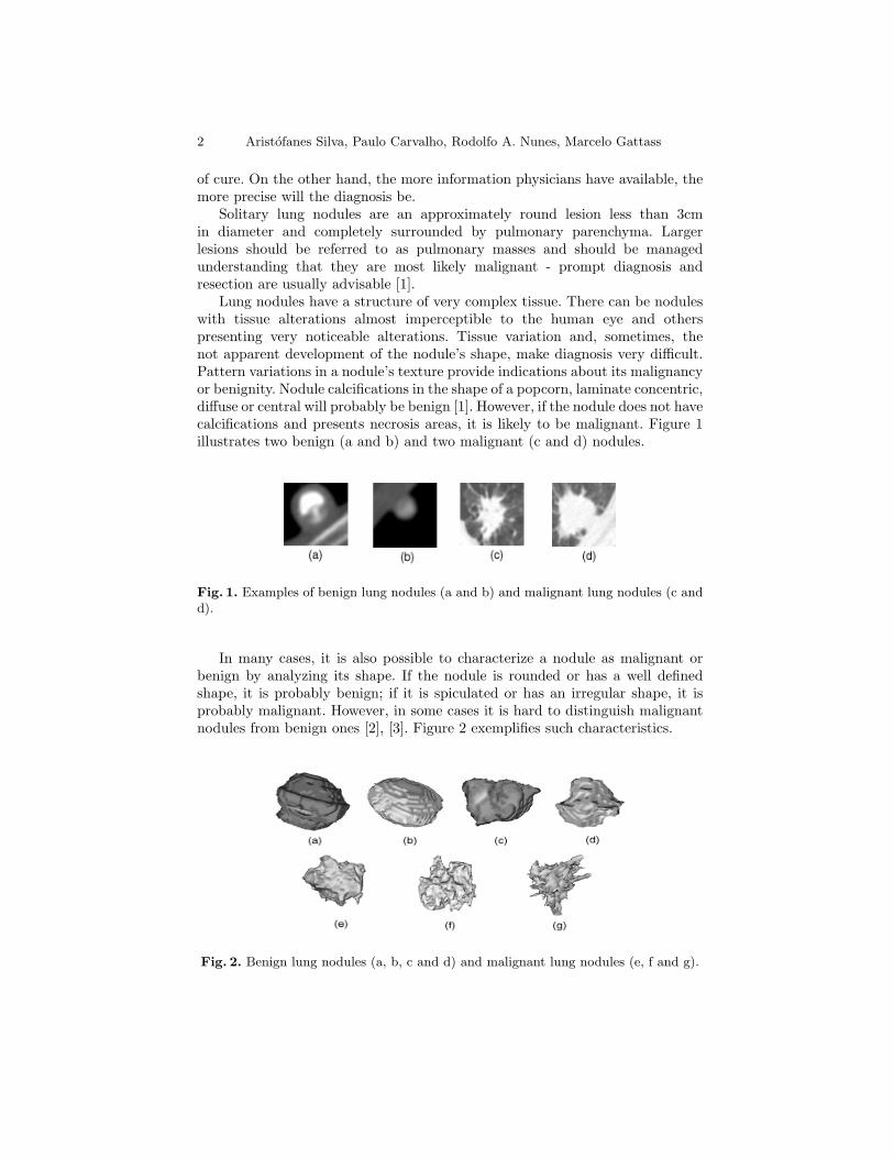
Lung nodules have a structure of very complex tissue. There can be noduleswith tissue alterations almost imperceptible to the human eye and otherspresenting very noticeable alterations. Tissue variation and, sometimes, thenot apparent development of the nodule’s shape, make diagnosis very difficult.Pattern variations in a nodule’s texture provide indications about its malignancyor benignity. Nodule calcifications in the shape of a popcorn, laminate concentric,diffuse or central will probably be benign [1]. However, if the nodule does not havecalcifications and presents necrosis areas, it is likely to be malignant. Figure 1illustrates two benign (a and b) and two malignant (c and d) nodules.
Fig. 1. Examples of benign lung nodules (a and b) and malignant lung nodules (c andd).
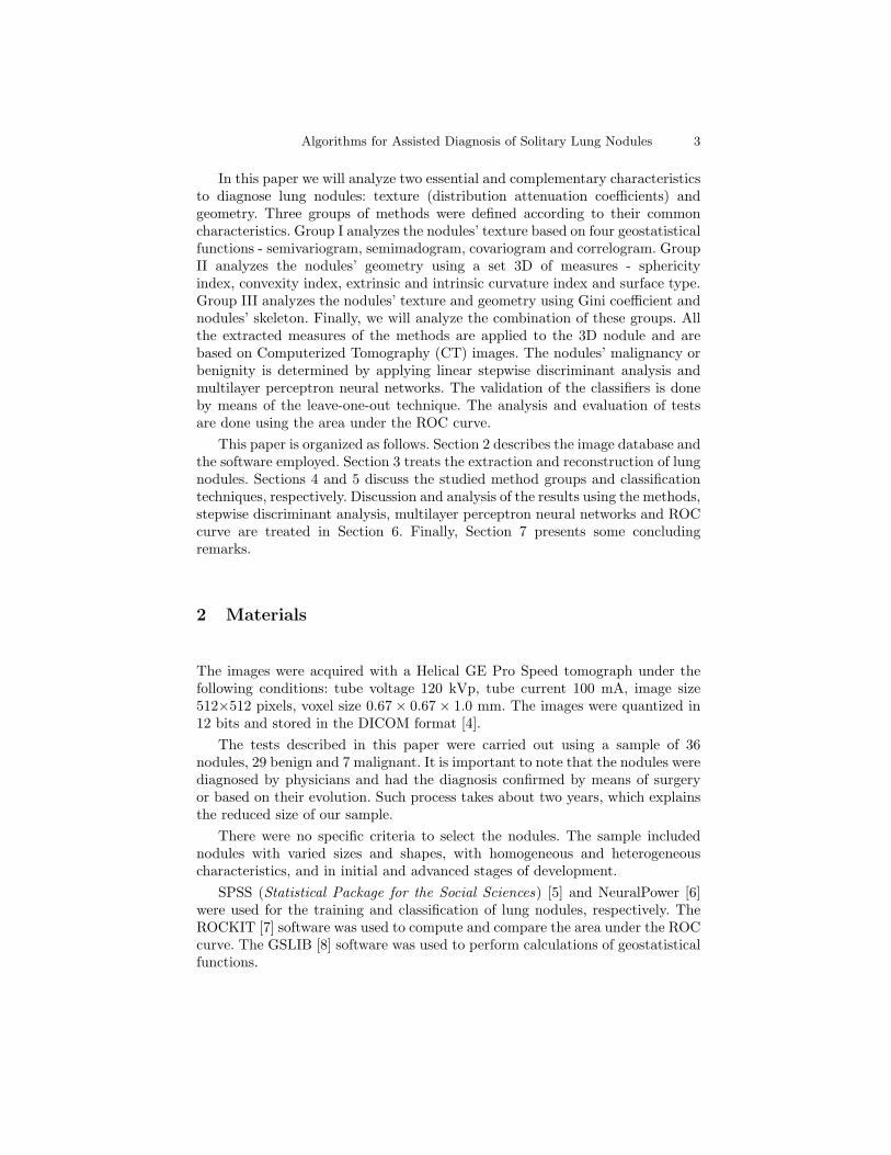
In many cases, it is also possible to characterize a nodule as malignant orbenign by analyzing its shape. If the nodule is rounded or has a well definedshape, it is probably benign; if it is spiculated or has an irregular shape, it isprobably malignant. However, in some cases it is hard to distinguish malignantnodules from benign ones [2], [3]. Figure 2 exemplifies such characteristics.
Fig. 2. Benign lung nodules (a, b, c and d) and malignant lung nodules (e, f and g).
Algorithms for Assisted Diagnosis of Solitary Lung Nodules 3
In this paper we will analyze two essential and complementary characteristicsto diagnose lung nodules: texture (distribution attenuation coefficients) andgeometry. Three groups of methods were defined according to their commoncharacteristics. Group I analyzes the nodules’ texture based on four geostatisticalfunctions - semivariogram, semimadogram, covariogram and correlogram. GroupII analyzes the nodules’ geometry using a set 3D of measures - sphericityindex, convexity index, extrinsic and intrinsic curvature index and surface type.Group III analyzes the nodules’ texture and geometry using Gini coefficient andnodules’ skeleton. Finally, we will analyze the combination of these groups. Allthe extracted measures of the methods are applied to the 3D nodule and arebased on Computerized Tomography (CT) images. The nodules’ malignancy orbenignity is determined by applying linear stepwise discriminant analysis andmultilayer perceptron neural networks. The validation of the classifiers is doneby means of the leave-one-out technique. The analysis and evaluation of testsare done using the area under the ROC curve.
This paper is organized as follows. Section 2 describes the image database andthe software employed. Section 3 treats the extraction and reconstruction of lungnodules. Sections 4 and 5 discuss the studied method groups and classificationtechniques, respectively. Discussion and analysis of the results using the methods,stepwise discriminant analysis, multilayer perceptron neural networks and ROCcurve are treated in Section 6. Finally, Section 7 presents some concludingremarks.
2 Materials
The images were acquired with a Helical GE Pro Speed tomograph under thefollowing conditions: tube voltage 120 kVp, tube current 100 mA, image size512×512 pixels, voxel size 0.67× 0.67× 1.0 mm. The images were quantized in12 bits and stored in the DICOM format [4].
The tests described in this paper were carried out using a sample of 36nodules, 29 benign and 7 malignant. It is important to note that the nodules werediagnosed by physicians and had the diagnosis confirmed by means of surgeryor based on their evolution. Such process takes about two years, which explainsthe reduced size of our sample.
There were no specific criteria to select the nodules. The sample includednodules with varied sizes and shapes, with homogeneous and heterogeneouscharacteristics, and in initial and advanced stages of development.
SPSS (Statistical Package for the Social Sciences) [5] and NeuralPower [6]were used for the training and classification of lung nodules, respectively. TheROCKIT [7] software was used to compute and compare the area under the ROCcurve. The GSLIB [8] software was used to perform calculations of geostatisticalfunctions.
4 Aristofanes Silva, Paulo Carvalho, Rodolfo A. Nunes, Marcelo Gattass
3 3D Extraction and Reconstruction of Lung Nodules
In most cases, lung nodules are easy to be visually detected by physicians, sincetheir shape and location are different from other lung structures. However, thenodules’ voxel density is similar to that of other structures, such as blood vessels,which makes automatic computer detection difficult. This happens especiallywhen a nodule is adjacent to the pleura. For this reason, we have used the 3Dregion-growing algorithm with voxel aggregation [9], which provides physiciansgreater interactivity and control over the segmentation and determination ofrequired parameters (thresholds, initial and final slice, and seed).
Two other resources help and provide greater control in the segmentationprocedure: the barrier and the eraser. The barrier is a cylinder placed aroundthe nodule by the user with the purpose of restricting the region of interestand stopping the segmentation by voxel aggregation from invading other lungstructures. The eraser is a resource of the system that allows physicians to eraseundesired structures, either before or after segmentation, in order to avoid andcorrect segmentation errors [10].
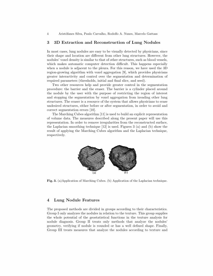
The Marching Cubes algorithm [11] is used to build an explicit representationof volume data. The measures described along the present paper will use thisrepresentation. In order to remove irregularities from the reconstructed surface,the Laplacian smoothing technique [12] is used. Figures 3 (a) and (b) show theresult of applying the Marching Cubes algorithm and the Laplacian technique,respectively.
Fig. 3. (a)Application of Marching Cubes. (b) Application of the Laplacian technique.
4 Lung Nodule Features
The proposed methods are divided in groups according to their characteristics.Group I only analyzes the nodules in relation to the texture. This group suppliesthe whole potential of the geostatistical functions in the texture analysis fornodule diagnosis. Group II treats only methods that analyze the nodules’geometry, verifying if nodule is rounded or has a well defined shape. Finally,Group III treats measures that analyze the nodules according to texture and
Algorithms for Assisted Diagnosis of Solitary Lung Nodules 5
geometry aspects. This group includes combined methods based on the twocharacteristics in order to obtain more information.
4.1 Geostatistical Functions – Group I
The semivariogram, semimadogram, covariogram, and correlogram functionssummarize the strength of associations between responses as a function ofdistance, and possibly direction [13], [14], [15]. We typically assume that spatialautocorrelation does not depend on where a pair of observations (in our case,voxel or attenuation coefficient) is located, but only on the distance between thetwo observations, and possibly on the direction of their relative displacement.
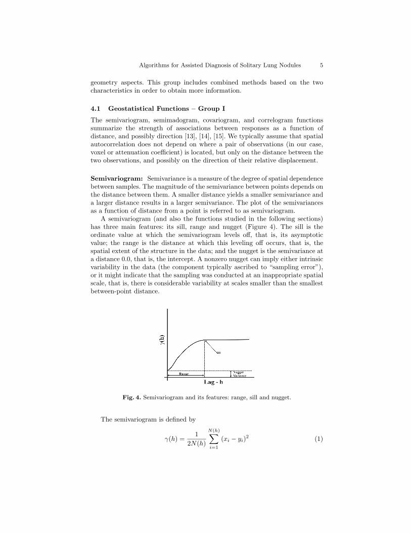
Semivariogram: Semivariance is a measure of the degree of spatial dependencebetween samples. The magnitude of the semivariance between points depends onthe distance between them. A smaller distance yields a smaller semivariance anda larger distance results in a larger semivariance. The plot of the semivariancesas a function of distance from a point is referred to as semivariogram.
A semivariogram (and also the functions studied in the following sections)has three main features: its sill, range and nugget (Figure 4). The sill is theordinate value at which the semivariogram levels off, that is, its asymptoticvalue; the range is the distance at which this leveling off occurs, that is, thespatial extent of the structure in the data; and the nugget is the semivariance ata distance 0.0, that is, the intercept. A nonzero nugget can imply either intrinsicvariability in the data (the component typically ascribed to “sampling error”),or it might indicate that the sampling was conducted at an inappropriate spatialscale, that is, there is considerable variability at scales smaller than the smallestbetween-point distance.
Fig. 4. Semivariogram and its features: range, sill and nugget.
The semivariogram is defined by
γ(h) =1
2N(h)
N(h)∑i=1
(xi − yi)2 (1)
6 Aristofanes Silva, Paulo Carvalho, Rodolfo A. Nunes, Marcelo Gattass
where h is the lag (vector) distance between the head value (source voxel), yi,and the tail value (target voxel), xi, and N(h) is the number of pairs at lag h.
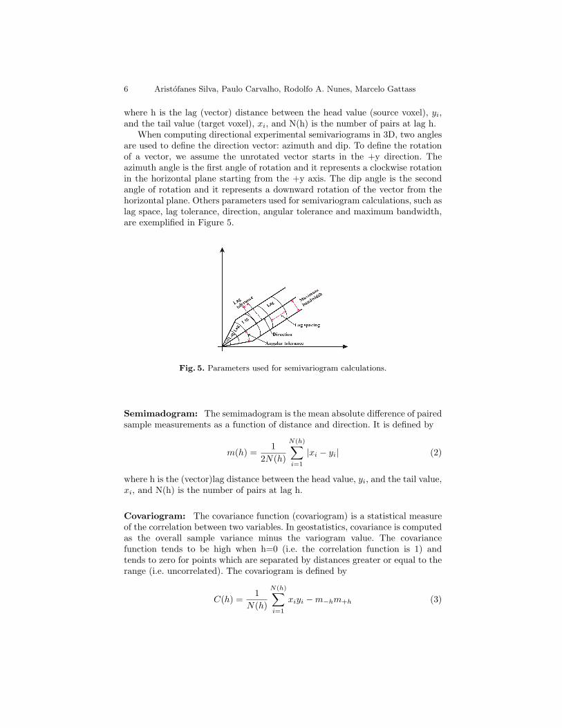
When computing directional experimental semivariograms in 3D, two anglesare used to define the direction vector: azimuth and dip. To define the rotationof a vector, we assume the unrotated vector starts in the +y direction. Theazimuth angle is the first angle of rotation and it represents a clockwise rotationin the horizontal plane starting from the +y axis. The dip angle is the secondangle of rotation and it represents a downward rotation of the vector from thehorizontal plane. Others parameters used for semivariogram calculations, such aslag space, lag tolerance, direction, angular tolerance and maximum bandwidth,are exemplified in Figure 5.
Fig. 5. Parameters used for semivariogram calculations.
Semimadogram: The semimadogram is the mean absolute difference of pairedsample measurements as a function of distance and direction. It is defined by
m(h) =1
2N(h)
N(h)∑i=1
|xi − yi| (2)
where h is the (vector)lag distance between the head value, yi, and the tail value,xi, and N(h) is the number of pairs at lag h.
Covariogram: The covariance function (covariogram) is a statistical measureof the correlation between two variables. In geostatistics, covariance is computedas the overall sample variance minus the variogram value. The covariancefunction tends to be high when h=0 (i.e. the correlation function is 1) andtends to zero for points which are separated by distances greater or equal to therange (i.e. uncorrelated). The covariogram is defined by
C(h) =1
N(h)
N(h)∑i=1
xiyi −m−hm+h (3)
Algorithms for Assisted Diagnosis of Solitary Lung Nodules 7
where m−h is the mean of the tail values,
m−h =1
N(h)
N(h)∑i=1
xi (4)
and m+h is the mean of the head values,
m+h =1
N(h)
N(h)∑i=1
yi (5)
Correlogram: The correlation function (correlogram) is a standardized versionof the covariance function; the correlation coefficients range from -1 to 1. Thecorrelation is expected to be high for units which are close to each other(correlation = 1 at distance zero) and tends to zero as the distance betweenunits increases. The correlation is defined by
ρ(h) =C(h)
σ−hσ+h(6)
where σ−h is the standard deviation of tail values,
σ−h =
1N(h)
N(h)∑i=1
x2i −m2
−h
12
(7)
and σ+h is the standard deviation of head values,
σ+h =
1N(h)
N(h)∑i=1
x2i −m2
+h
12
(8)
4.2 Geometry Methods – Group II
The measures to be presented in this section seek to capture information on thenodule’s 3D geometry from the CT. The measures should ideally be invariantto changes in the image’s parameters, such as voxel size, orientation and slicethickness.
Sphericity Index: The Sphericity Index (SI ) measures the nodule’s behaviorin relation to a spherical object. It is defined as
SI =6√
πV
A32
(9)
where V is the surface volume and A corresponds to the surface area. Thus, ifthe nodule’s shape is similar to a sphere, the value will be close to 1. In all cases,SI ≤ 1.
8 Aristofanes Silva, Paulo Carvalho, Rodolfo A. Nunes, Marcelo Gattass
Convexity Index: The Convexity Index (CI ) [16] measures the degree ofconvexity, defined as the area of the surface of object B (A(B)) divided by thearea of the surface of its convex hull (A(HB)). That is,
CI =A(B)
A(HB)(10)
The more convex the object is, the closer the value of CI will be to 1. For allobjects, CI ≥ 1.
Curvature Index: The two measures presented below are based on the maincurvatures kmin and kmax, defined by
kmin,max = H ∓√
H2 −K (11)
where K and H are the Gaussian and mean curvatures, respectively. The valuesof H and K are estimated using the methods described by [17].
a) Intrinsic curvature: The Intrinsic Curvature Index (ICI ) [16], [17] capturesinformation on the properties of the surface’s intrinsic curvatures, and isdefined as
ICI =14π
∫ ∫|kminkmax|dA (12)
Any undulation or salience on the surface with the shape of half a sphereincrements the Intrinsic Curvature Index by 0.5, regardless of its size - thatis, the ICI counts the number of regions with undulations or saliencies onthe surface being analyzed.
b) Extrinsic curvature: The Extrinsic Curvature Index (ECI ) [16], [17] capturesinformation on the properties of the surface’s extrinsic curvatures, and isdefined as
ECI =14π
∫ ∫|kmax| (|kmax| − |kmin|) dA (13)
Any crack or gap with the shape of half a cylinder increments the ECI inproportion to its length, starting at 0.5 if its length is equal to its diameter -that is, the ECI counts the number and length (in relation to the diameter)of semicylindrical cracks or gaps on the surface.
Types of Surfaces: With the values of extrinsic (H) and intrinsic (K)curvatures, it is possible to specify eight basic types of surfaces [18], [19]: peak(K > 0 and H < 0), pit (K > 0 and H > 0), ridge (K = 0 and H < 0), flat(K = 0 and H = 0), valley (K = 0 and H > 0), saddle valley (K < 0 andH > 0), minimal (K < 0 and H = 0), saddle ridge (K < 0 and H < 0).
The measures described below were presented in the work by [20] for theclassification of lung nodules and the results were promising. However, they havecomputed curvatures H and K directly from the voxel intensity values, while
Algorithms for Assisted Diagnosis of Solitary Lung Nodules 9
here we compute them in relation to the extracted surface, which is composedby triangles.
In practice, it is difficult to determine values that are exactly equal to zero,due to numerical precision. Therefore we have selected only types peak, pit, saddlevalley and saddle ridge for our analysis [20].
a) Amount of each Surface Type:This measure indicates the relative frequency of each type of surface in thenodule, with APK (Amount of peak surface), API (Amount of pit surface),ASR (Amount of saddle ridge surface) and ASV (Amount of saddle valleysurface).
b) Area Index for each Surface Type:For each surface type, the area occupied in the nodule divided by the totalnodule area is computed, with AIPK (Area Index for peak surface), AIPI(Area Index for pit surface), AISR (Area Index for saddle ridge surface) andAISV (Area Index for saddle valley surface).
c) Mean Curvedness for each Surface Type:Curvedness is a positive number that measures the curvature amount orintensity on the surface [18]:
c =
√k2min + k2
max
2(14)
The measures are based on the curvedness and the surface types. For eachsurface type, the mean curvedness is determined using the curvedness ofeach surface type, divided by the curvedness number in each surface type,with CPK (mean curvedness for peak), CPI (mean curvedness for pit), CSR(mean curvedness for saddle ridge) and CSV (mean curvedness for saddlevalley).
4.3 Geometry and Texture Methods – Group III
This section will deal with two methods, Gini coefficient and the nodules’skeleton, which implicitly get characteristics of the nodules’ texture andgeometry.
Gini Coefficient Applied to 3D Texture: The study of inequality inthe distribution of a given variable in a population has received constantattention in the past few years. In the economic domain, the pioneering worksreferred to inequality in income distribution, but many of the methodologiesdeveloped for the analysis of this important issue were later generalized to amultiplicity of phenomena, either in the economic domain or in other areasof application [21]. Classical examples are the study of the distribution ofwealth [22], production [23], health [24], education [25], of the greatest or smallestconcentration of clients in a company [26], etc.
10 Aristofanes Silva, Paulo Carvalho, Rodolfo A. Nunes, Marcelo Gattass
Based on such domains of application, many concentration measures wereproposed. Since it is not our purpose here to list all these measures, we will onlydescribe the Lorenz curve and the coefficient that is associated to it, the Ginicoefficient, which are more relevant to the present work.
In this work, we will use the Lorenz curve and the Gini coefficient to analyzethe degree of voxel density concentration in lung nodules. For instance, when anodule contains calcifications (probably benign cases) we expect voxel densityto be concentrated at such locations. As we will see below, the Lorenz curve andthe Gini coefficient should reflect this fact.
Lorenz CurveThe Lorenz curve is a graphical representation of the cumulative distribution ofa given attribute in a population. To build the Lorenz curve, the elements aresorted with respect to the value Xi of that attribute, from the smallest attributevalue to the largest. Then, each element is plotted according to its relative rankpi and the corresponding cumulative percentage qi of the attribute under study.More precisely, for each i = 1, 2, 3, ..., n:
pi =i
n(15)
qi =
i∑j=1
Xj
n∑j=1
Xj
(16)
where n is the number of elements and Xj is the value of the attribute for theelement of order j.
The Lorenz curve is then compared to the perfect equality line, whichcorresponds to the case where each element has the same share of the attributein the population. In this case, qi = pi = i
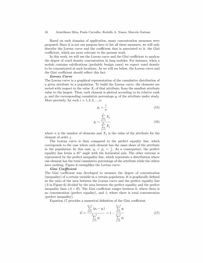
n . As a consequence, the perfectequality line forms a 45◦ angle with the horizontal axis. The other extreme isrepresented by the perfect inequality line, which represents a distribution whereone element has the total cumulative percentage of the attribute while the othershave nothing. Figure 6 exemplifies the Lorenz curve.
Gini CoefficientThe Gini coefficient was developed to measure the degree of concentration(inequality) of a certain variable in a certain population. It is graphically definedas the ratio of the area between the Lorenz curve and the perfect equality line(A in Figure 6) divided by the area between the perfect equality and the perfectinequality lines (A + B). The Gini coefficient ranges between 0, where there isno concentration (perfect equality), and 1, where there is total concentration(perfect inequality).
Equation 17 provides a numerical definition of the Gini coefficient.
G =
n−1∑i=1
(pi − qi)
n−1∑i=1
pi
= 1−
n−1∑i=1
qi
n−1∑i=1
pi
(17)
Algorithms for Assisted Diagnosis of Solitary Lung Nodules 11
Fig. 6. Example of Lorenz Curve and Gini coefficient (A/(A + B)).
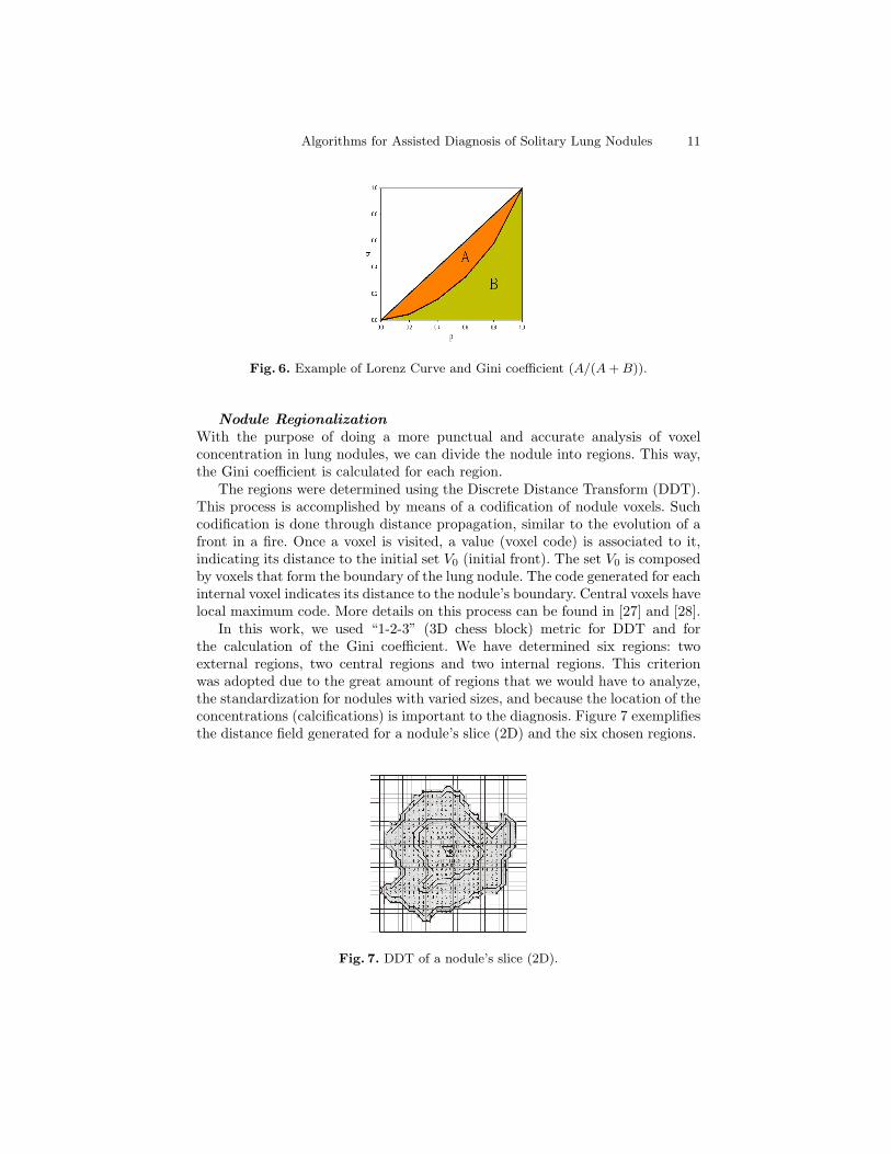
Nodule RegionalizationWith the purpose of doing a more punctual and accurate analysis of voxelconcentration in lung nodules, we can divide the nodule into regions. This way,the Gini coefficient is calculated for each region.
The regions were determined using the Discrete Distance Transform (DDT).This process is accomplished by means of a codification of nodule voxels. Suchcodification is done through distance propagation, similar to the evolution of afront in a fire. Once a voxel is visited, a value (voxel code) is associated to it,indicating its distance to the initial set V0 (initial front). The set V0 is composedby voxels that form the boundary of the lung nodule. The code generated for eachinternal voxel indicates its distance to the nodule’s boundary. Central voxels havelocal maximum code. More details on this process can be found in [27] and [28].
In this work, we used “1-2-3” (3D chess block) metric for DDT and forthe calculation of the Gini coefficient. We have determined six regions: twoexternal regions, two central regions and two internal regions. This criterionwas adopted due to the great amount of regions that we would have to analyze,the standardization for nodules with varied sizes, and because the location of theconcentrations (calcifications) is important to the diagnosis. Figure 7 exemplifiesthe distance field generated for a nodule’s slice (2D) and the six chosen regions.
Fig. 7. DDT of a nodule’s slice (2D).
12 Aristofanes Silva, Paulo Carvalho, Rodolfo A. Nunes, Marcelo Gattass
Skeleton Measures: Skeletonization is a convenient tool to obtain a simplifiedrepresentation of shapes that preserves most topological information [29]. Askeleton captures the local symmetry axes and is therefore centered in theobject. In image analysis, features extracted from skeletons are commonly used inpattern-recognition algorithms [30]. Skeletons contain information about shapefeatures which are very important in the context this work.
We will use Zhou and Toga’s algorithm [31] in the skeletonization process.They have proposed a voxel-coding approach to efficiently skeletonize volumetricobjects. Each object point has two codes. One is the Boundary Seeded code (BS),which coincides with the traditional distance transform to indicate the minimumdistance to the object’s boundary. The second code is the so-called Single Seededcode (SS), which indicates the distance to a specific reference point. SS code isused to extract the shortest path between a point in the object and the referencepoint. These paths are represented by sequential sets of voxels that will composethe initial skeleton. The key idea of voxel coding is to use the SS codes to generatea connected raw skeleton and the BS codes to assure the centeredness of the finalskeleton.
We have extracted seven measures based on skeletons to analyze lung nodules:
a) Number of Segments (NS)b) Number of Branches (NB)c) Fraction of Volume (FV): FV is defined by
FV =v
V(18)
where v is the skeleton volume and V is the lung nodule’s volume.d) Length of Segments (LS):
LS =L3√
V(19)
where L is the length of all segments and V is the lung nodule’s volume.e) Volume of Convex Hull (VCH)f) Rate between the number of segments and the volume of the convex hull
(NSVCH)[30]
NSV CH =NS
V CH(20)
g) Variation Coefficient (VC) of the N larger segments in the skeleton. The valueof N is defined based on the skeleton with the smallest number of segmentsamong all skeletons analyzed. The variation coefficient is dimensionless andscale-independent. A high VC indicates high variability in the skeleton’ssegment. The VC is a measure of relative dispersion and is given by
V C =σ
µ(21)
where σ is the standard deviation and µ is the mean.
Algorithms for Assisted Diagnosis of Solitary Lung Nodules 13
h) Histogram Moments (variance (M2), skewness (M3), kurtosis (M4)) of theN largest segments in the skeleton. The value of N is defined based on theskeleton with the smallest number of segments among all skeletons analyzed.Three gray-level histogram moments are extracted from the voxel valuehistogram of each skeleton’s segment, and are defined as follows:
Mn =∑
(xi − µ)nfi
N(22)
where n = 2, 3, 4 , µ is the mean, N denotes the number of voxels in thesegment, and fi is the histogram.More detailed information on moment theory can be found in [32].
5 Classification Algorithms
A a wide variety of approaches have been taken towards the classification task.Three main historical strands of research can be identified [33]: statistical, neuralnetwork and machine learning. This section provides an overview of Fisher’sLinear Discriminant Analysis and Multilayer Perceptron based on the first twoparadigms mentioned above.
5.1 Fisher’s Linear Discriminant Analysis - FLDA
Linear discrimination, as the name suggests, looks for linear combinations of theinput variables that can provide an adequate separation for the given classes.Rather than to look for a particular parametric form of distribution, LDA usesan empirical approach to define linear decision planes in the attribute space,i.e., it models a surface. The discriminant functions used by LDA are built upas a linear combination of the variables that seek to somehow maximize thedifferences between the classes [34]:
y = β1x1 + β2x2 + · · ·+ βnxn = β′x (23)
The problem then is reduced to finding a suitable vector β. There are severalpopular variations of this idea, one of the most successful being the Fisher LinearDiscriminant Rule. Fisher’s Rule is considered a “sensible” classification, in thesense that it is intuitively appealing. It makes use of the fact that distributionsthat have greater variance between their classes than within each class shouldbe easier to separate. Therefore, it searches for a linear function in the attributespace that maximizes the ratio of the between-group sum-of-squares (B) to thewithin-group sum-of-squares (W ). This can be achieved by maximizing the ratio
β′Bβ
β′Wβ(24)
and it turns out that the vector that maximizes this ratio, β, is the eigenvectorcorresponding to the largest eigenvalue of W−1B, i.e., the linear discriminant
14 Aristofanes Silva, Paulo Carvalho, Rodolfo A. Nunes, Marcelo Gattass
function y is equivalent to the first canonical variate. Hence the discriminantrule can be written as:
x ∈ i if∣∣βT x− βT ui
∣∣ <∣∣βT x− βT uj
∣∣ , for all j 6= i (25)
where W =∑
niSi and B =∑
ni(xi − x)(xi − x)′, and ni is class i sample size,
Si is class i covariance matrix, xi is the class i mean sample value and x is thepopulation mean.
Stepwise discriminant analysis [34] was used to select the best variablesto differentiate between groups. These measures were used by Fisher’s LinearDiscriminant Analysis and Multilayer Perceptron Neural Networks classifiers.
5.2 Multilayer Perceptron Neural Networks
The Multilayer Perceptron - MLP, a feed-forward back-propagationnetwork, is the most frequently used neural network technique in patternrecognition [35], [36]. Briefly, MLPs are supervised learning classifiers thatconsist of an input layer, an output layer, and one or more hidden layers thatextract useful information during learning and assign modifiable weightingcoefficients to components of the input layers. In the first (forward) pass,weights assigned to the input units and the nodes in the hidden layers andbetween the nodes in the hidden layer and the output, determine the output.The output is compared with the target output. An error signal is then backpropagated and the connection weights are adjusted correspondingly. Duringtraining, MLPs construct a multidimensional space, defined by activation ofthe hidden nodes, so that the two classes (benign and malignant nodules) areas separable as possible. The separating surface adapts to the data.
5.3 Validating and Evaluating Classification Methods
In order to validate the classificatory power of the discriminant function,the leave-one-out technique [37] was employed. Through this technique, thecandidate nodules from 35 cases in our database were used to train the classifier;the trained classifier was then applied to the candidate nodules in the remainingcase. This technique was repeated until all 36 cases in our database had beenthe “remaining” case.
In order to evaluate the ability of the classifier to differentiate benignfrom malignant nodules, the area (AUC) under the ROC (Receiver OperatingCharacteristic) [38] curve was used. In other words, the ROC curve describesthe ability of the classifiers to correctly differentiate the set of lung nodulecandidates into two classes, based on the true-positive fraction (sensitivity) andfalse-positive fraction (1-specificity). Sensitivity is defined by TP/(TP + FN),specificity is defined by TN/(TN + FP ), and accuracy is defined by (TP +TN)/(TP +TN +FP +FN), where TN is true-negative, FN is false-negative,FP is false-positive, and TP is true-positive.
Algorithms for Assisted Diagnosis of Solitary Lung Nodules 15
6 Results
This section shows the results of applying the proposed methods and classifyingbetween malignant and benign lung nodules.
6.1 Application of Methods
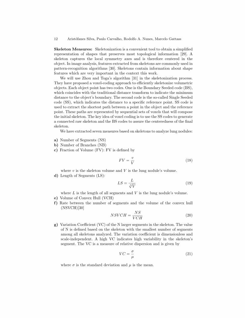
Geostatistical Functions – Group I: Figure 8 shows the application ofexperimental semivariograms to volumes represented by Figures 1(a), (b), (c)and (d). We can notice that benign nodules have the sill higher than malignantnodules, and that the initial slope is much more accentuated. The graph analysisshows the presence of greater dispersion in benign nodules than in malignantnodules.
Fig. 8. Semivariogram applied to the example in Figure 1.
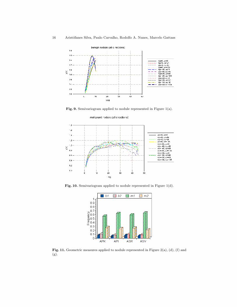
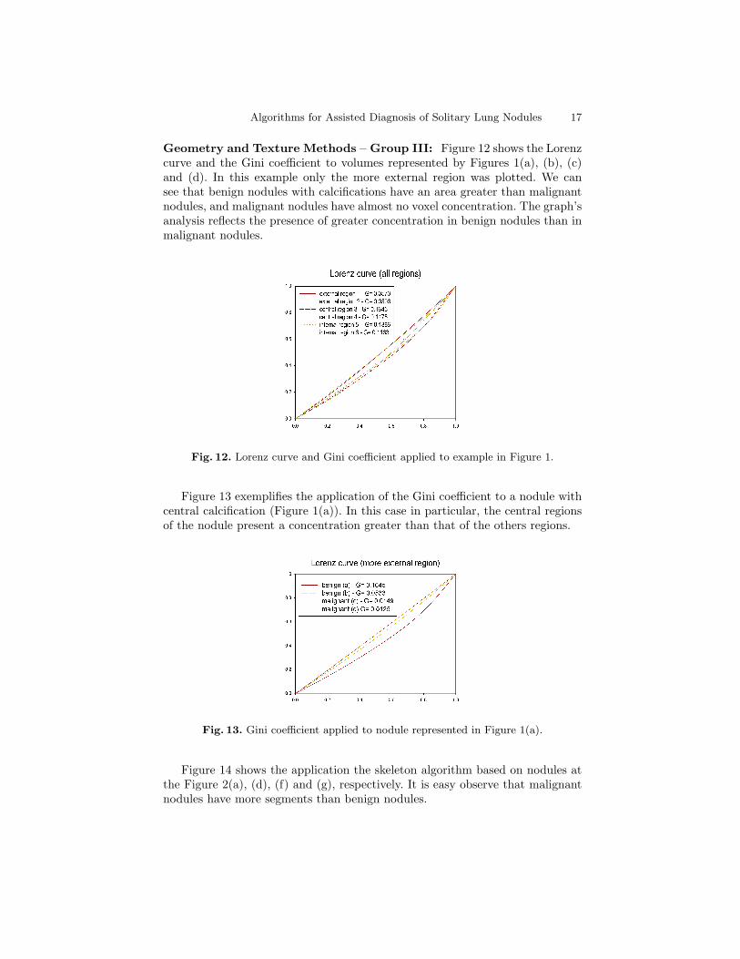
Figures 9 and 10 exemplify, respectively, the application of the semivariogramfunction to a benign nodule (Figure 1(a)) and a malignant nodule Figure 1(d)).The graph’s curves show the calculated variance in twelve specified directions,in relation the several distances.
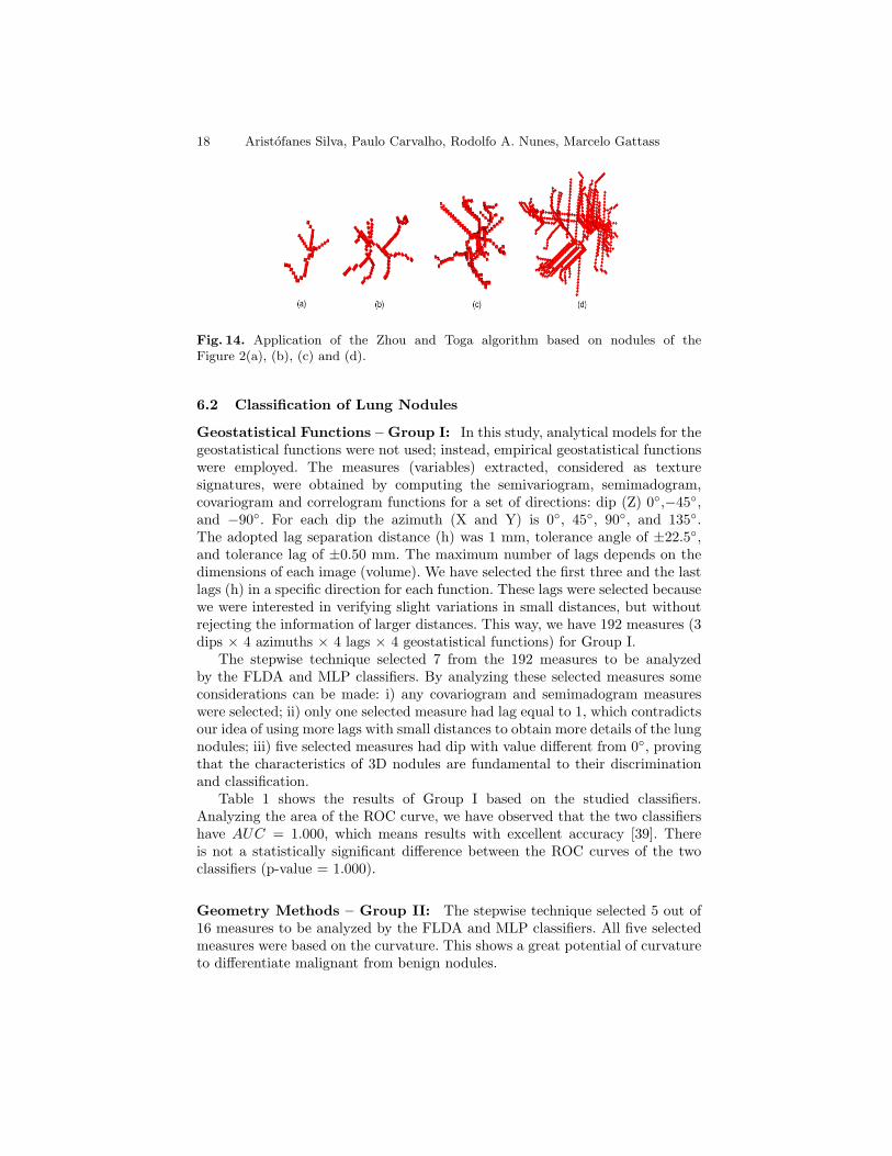
Geometry Methods – Group II: Figure 11 shows the application of only4 to the 16 geometric measures presented related to the curvature: APK, API,ASR and ASV. In the Figure 11, b1 and b2 are benign nodules represented byFigures 2(a) and (d), and m1 and m2 are malignant nodules represented byFigures 2(f) and (g). This Figure shows that the largest number of occurrencescorresponds to the malignant nodule (m1 ), followed by the nodule (m2 ), thenby the benign nodule (b2 ), and last by the benign nodule (b1 ). This fact isexplained by the largest amount of ramifications (curvatures) presented by themalignant nodules. In this example, the analyzed measures correctly separatedbenign from malignant lung nodules.
16 Aristofanes Silva, Paulo Carvalho, Rodolfo A. Nunes, Marcelo Gattass
Fig. 9. Semivariogram applied to nodule represented in Figure 1(a).
Fig. 10. Semivariogram applied to nodule represented in Figure 1(d).
Fig. 11. Geometric measures applied to nodule represented in Figure 2(a), (d), (f) and(g).
Algorithms for Assisted Diagnosis of Solitary Lung Nodules 17
Geometry and Texture Methods – Group III: Figure 12 shows the Lorenzcurve and the Gini coefficient to volumes represented by Figures 1(a), (b), (c)and (d). In this example only the more external region was plotted. We cansee that benign nodules with calcifications have an area greater than malignantnodules, and malignant nodules have almost no voxel concentration. The graph’sanalysis reflects the presence of greater concentration in benign nodules than inmalignant nodules.
Fig. 12. Lorenz curve and Gini coefficient applied to example in Figure 1.
Figure 13 exemplifies the application of the Gini coefficient to a nodule withcentral calcification (Figure 1(a)). In this case in particular, the central regionsof the nodule present a concentration greater than that of the others regions.
Fig. 13. Gini coefficient applied to nodule represented in Figure 1(a).
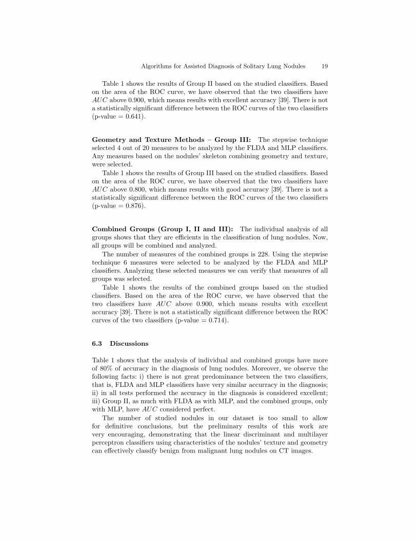
Figure 14 shows the application the skeleton algorithm based on nodules atthe Figure 2(a), (d), (f) and (g), respectively. It is easy observe that malignantnodules have more segments than benign nodules.
18 Aristofanes Silva, Paulo Carvalho, Rodolfo A. Nunes, Marcelo Gattass
Fig. 14. Application of the Zhou and Toga algorithm based on nodules of theFigure 2(a), (b), (c) and (d).
6.2 Classification of Lung Nodules
Geostatistical Functions – Group I: In this study, analytical models for thegeostatistical functions were not used; instead, empirical geostatistical functionswere employed. The measures (variables) extracted, considered as texturesignatures, were obtained by computing the semivariogram, semimadogram,covariogram and correlogram functions for a set of directions: dip (Z) 0◦,−45◦,and −90◦. For each dip the azimuth (X and Y) is 0◦, 45◦, 90◦, and 135◦.The adopted lag separation distance (h) was 1 mm, tolerance angle of ±22.5◦,and tolerance lag of ±0.50 mm. The maximum number of lags depends on thedimensions of each image (volume). We have selected the first three and the lastlags (h) in a specific direction for each function. These lags were selected becausewe were interested in verifying slight variations in small distances, but withoutrejecting the information of larger distances. This way, we have 192 measures (3dips × 4 azimuths × 4 lags × 4 geostatistical functions) for Group I.
The stepwise technique selected 7 from the 192 measures to be analyzedby the FLDA and MLP classifiers. By analyzing these selected measures someconsiderations can be made: i) any covariogram and semimadogram measureswere selected; ii) only one selected measure had lag equal to 1, which contradictsour idea of using more lags with small distances to obtain more details of the lungnodules; iii) five selected measures had dip with value different from 0◦, provingthat the characteristics of 3D nodules are fundamental to their discriminationand classification.
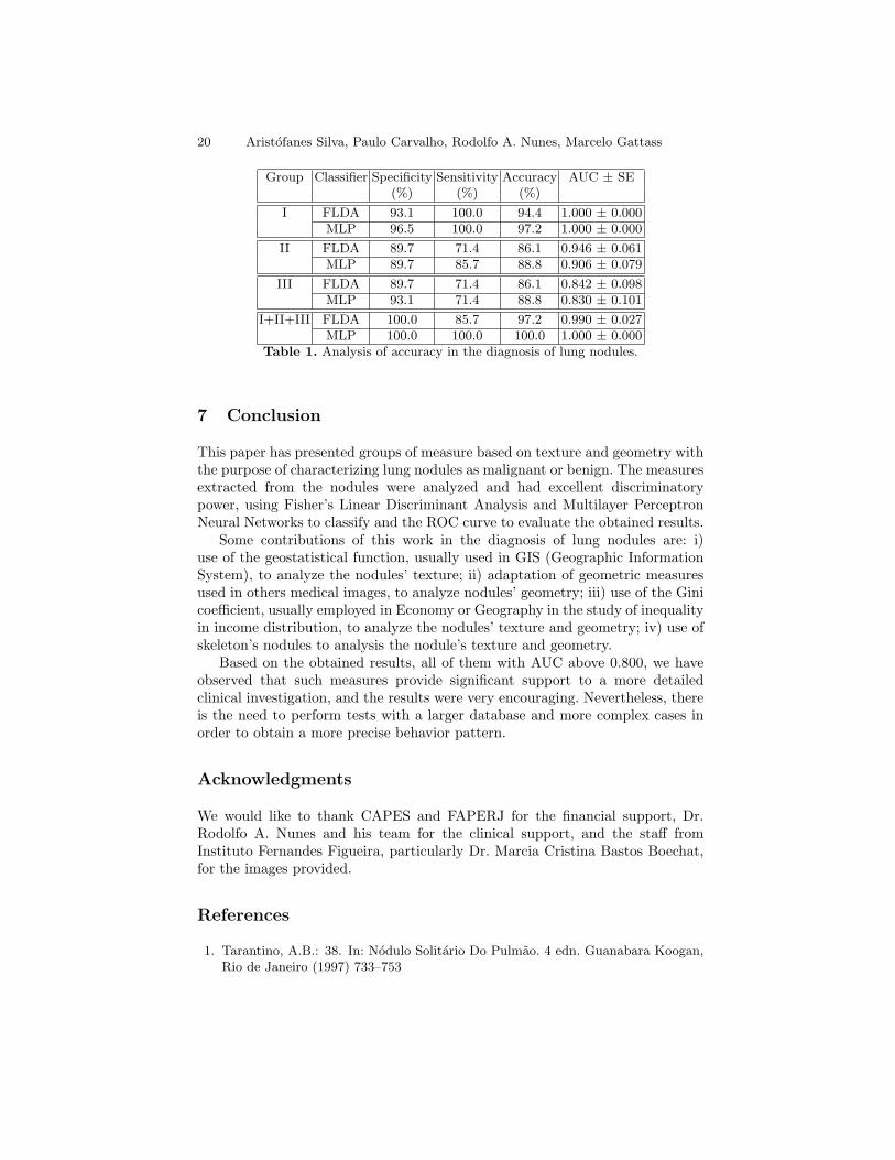
Table 1 shows the results of Group I based on the studied classifiers.Analyzing the area of the ROC curve, we have observed that the two classifiershave AUC = 1.000, which means results with excellent accuracy [39]. Thereis not a statistically significant difference between the ROC curves of the twoclassifiers (p-value = 1.000).
Geometry Methods – Group II: The stepwise technique selected 5 out of16 measures to be analyzed by the FLDA and MLP classifiers. All five selectedmeasures were based on the curvature. This shows a great potential of curvatureto differentiate malignant from benign nodules.
Algorithms for Assisted Diagnosis of Solitary Lung Nodules 19
Table 1 shows the results of Group II based on the studied classifiers. Basedon the area of the ROC curve, we have observed that the two classifiers haveAUC above 0.900, which means results with excellent accuracy [39]. There is nota statistically significant difference between the ROC curves of the two classifiers(p-value = 0.641).
Geometry and Texture Methods – Group III: The stepwise techniqueselected 4 out of 20 measures to be analyzed by the FLDA and MLP classifiers.Any measures based on the nodules’ skeleton combining geometry and texture,were selected.
Table 1 shows the results of Group III based on the studied classifiers. Basedon the area of the ROC curve, we have observed that the two classifiers haveAUC above 0.800, which means results with good accuracy [39]. There is not astatistically significant difference between the ROC curves of the two classifiers(p-value = 0.876).
Combined Groups (Group I, II and III): The individual analysis of allgroups shows that they are efficients in the classification of lung nodules. Now,all groups will be combined and analyzed.
The number of measures of the combined groups is 228. Using the stepwisetechnique 6 measures were selected to be analyzed by the FLDA and MLPclassifiers. Analyzing these selected measures we can verify that measures of allgroups was selected.
Table 1 shows the results of the combined groups based on the studiedclassifiers. Based on the area of the ROC curve, we have observed that thetwo classifiers have AUC above 0.900, which means results with excellentaccuracy [39]. There is not a statistically significant difference between the ROCcurves of the two classifiers (p-value = 0.714).
6.3 Discussions
Table 1 shows that the analysis of individual and combined groups have moreof 80% of accuracy in the diagnosis of lung nodules. Moreover, we observe thefollowing facts: i) there is not great predominance between the two classifiers,that is, FLDA and MLP classifiers have very similar accurracy in the diagnosis;ii) in all tests performed the accuracy in the diagnosis is considered excellent;iii) Group II, as much with FLDA as with MLP, and the combined groups, onlywith MLP, have AUC considered perfect.
The number of studied nodules in our dataset is too small to allowfor definitive conclusions, but the preliminary results of this work arevery encouraging, demonstrating that the linear discriminant and multilayerperceptron classifiers using characteristics of the nodules’ texture and geometrycan effectively classify benign from malignant lung nodules on CT images.
20 Aristofanes Silva, Paulo Carvalho, Rodolfo A. Nunes, Marcelo Gattass
Group Classifier Specificity Sensitivity Accuracy AUC ± SE(%) (%) (%)
Table 1. Analysis of accuracy in the diagnosis of lung nodules.
7 Conclusion
This paper has presented groups of measure based on texture and geometry withthe purpose of characterizing lung nodules as malignant or benign. The measuresextracted from the nodules were analyzed and had excellent discriminatorypower, using Fisher’s Linear Discriminant Analysis and Multilayer PerceptronNeural Networks to classify and the ROC curve to evaluate the obtained results.
Some contributions of this work in the diagnosis of lung nodules are: i)use of the geostatistical function, usually used in GIS (Geographic InformationSystem), to analyze the nodules’ texture; ii) adaptation of geometric measuresused in others medical images, to analyze nodules’ geometry; iii) use of the Ginicoefficient, usually employed in Economy or Geography in the study of inequalityin income distribution, to analyze the nodules’ texture and geometry; iv) use ofskeleton’s nodules to analysis the nodule’s texture and geometry.
Based on the obtained results, all of them with AUC above 0.800, we haveobserved that such measures provide significant support to a more detailedclinical investigation, and the results were very encouraging. Nevertheless, thereis the need to perform tests with a larger database and more complex cases inorder to obtain a more precise behavior pattern.
Acknowledgments
We would like to thank CAPES and FAPERJ for the financial support, Dr.Rodolfo A. Nunes and his team for the clinical support, and the staff fromInstituto Fernandes Figueira, particularly Dr. Marcia Cristina Bastos Boechat,for the images provided.
References
1. Tarantino, A.B.: 38. In: Nodulo Solitario Do Pulmao. 4 edn. Guanabara Koogan,Rio de Janeiro (1997) 733–753
Algorithms for Assisted Diagnosis of Solitary Lung Nodules 21
2. Henschke, C.I., et al: Early lung cancer action project: A summary of the findingson baseline screening. The Oncologist 6 (2001) 147–152
3. Reeves, A.P., Kostis, W.J.: Computer-aided diagnosis for lung cancer. RadiologicClinics of North America 38 (2000) 497–509
Guide. Oxford University Press, New York (1992)9. Nikolaidis, N., Pitas, I.: 3-D Image Processing Algorithms. John Wiley, New York
(2001)10. Silva, A.C., Carvalho, P.C.P.: Sistema de analise de nodulo pulmonar. In: II
Workshop de Informatica aplicada a Saude, Itajai, Universidade de Itajai (2002)Avaliado em http://www.cbcomp.univali.br/pdf/2002/wsp035.pdf.
11. Lorensen, W.E., Cline, H.E.: Marching cubes: A high resolution 3D surfaceconstruction algorithm. Computer Graphics 21 (1987) 163–169
12. Ohtake, Y., Belyaev, A., Pasko, A.: Dynamic meshes for accurate polygonization ofimplicit surfaces with shape features. In Press, I.C.S., ed.: SMI 2001 InternationalConference on Shape Modeling and Applications. (2001) 74–81
13. Clark, I.: Practical Geostatistics. Applied Sience Publishers, London (1979)14. Cressie, N.A.C.: Statistical for Spatial Data. John Wiley & Sons, New York (1993)15. Journel, A.G., Huijbregts, C.J.: Mining Geostatistics. Academic Press, London
(1978)16. Smith, A.C.: The Folding of the Human Brain, from Shape to
Function. PhD thesis, University of London (1999) Available athttp://carmen.umds.ac.uk/a.d.smith/phd.html.
17. Essen, D.C.V., Drury, H.A.: Structural and functional analyses of human cerebralcortex using a surface-based atlas. The Journal of Neuroscience 17 (1997) 7079–7102
18. Koenderink, J.J.: Solid Shape. MIT Press, Cambridge, MA, USA (1990)19. Henderson, D.W.: Differental Geometry: A Geometric Introduction. Prentice-Hall,
Upper Saddle River, New Jersey (1998)20. Kawata, Y., Niki, N., , Ohmatsu, H., Kakinuma, R., Eguchi, K., Kaneko, M.,
Moriyama, N.: Classification of pulmonary nodules in thin-section CT imagesbased on shape characterization. In: International Conference on Image Processing.Volume 3., IEEE Computer Society Press (1997) 528–530
21. Houlding, S.W.: 3D Geoscience Modeling : Computer Techniques for GeologicalCharacterization. Springer-Verlag, Berlin (1994)
22. Ferreira, F.H., de Barros, R.P.: Education and income distribution in urban brazil,1976–1996. CEPAL Review 71 (2000) 43–64
23. Dahmani, A.: Changes to the oil export structure of opec member countries – ananalysis with the gini coefficient. OPEC Review 22 (1998) 277–290
24. Berndt, D.J., Fisher, J.W., Rajendrababu, R.V.: Measuring healthcare inequalitiesusing the gini index. In Press, I.C.S., ed.: 36th Hawaii International Conferenceon System Sciences (HICSS’03). (2003) 159 –168
25. Zhang, J., Li, T.: International inequality and convergence in educationalattainment, 1960–1990. Review of Development Economics 6 (2002) 383–392
22 Aristofanes Silva, Paulo Carvalho, Rodolfo A. Nunes, Marcelo Gattass
26. Lee, C.K., Kang, S.: Measuring earnings inequality and median earnings in thetourism industry. Tourism Management 19 (1998) 341–348
27. Peixoto, A., Carvalho, P.C.P.: Esqueletos de objetos volumetricos. TechnicalReport 34/00, Pontifıcia Universidade Catolica do Rio de Janeiro, Rio de Janeiro- Brasil (2000)
28. Peixoto, A., Velho, L.: Transformada de distancia. Technical Report 35/00,Pontifıcia Universidade Catolica do Rio de Janeiro, Rio de Janeiro - Brasil (2000)
29. Gonzalez, R.C., Woods, R.E.: Digital Image Processing. 3 edn. Addison-Wesley,Reading, MA, USA (1992)
30. da F. Costa, L., Velte, T.J.: Automatic characterization and classification ofglangion cells from the salamander retina. The Journal of Comparative Neurology404 (1999) 33–51
31. Zhou, Y., Toga, A.W.: Efficient skeletonization of volumetric objects. IEEETransactions on Visualization and Computer Graphics 5 (1999) 196–208
32. Sonka, M., Hlavac, V., Boyle, R.: Image Processing, Analysis and Machine Vision.2 edn. International Thomson Publishing (1998)
33. Michie, D., Spiegelhalter, D., Taylor, C., Speigelhalter, D.J.: Machine Learning,Neural and Statistical Classification. Ellis Horwood Series in Artificial Intelligence,NJ, USA (1994)
34. Lachenbruch, P.A.: Discriminant Analysis. Hafner Press, New York (1975)35. Duda, R.O., Hart, P.E.: Pattern Classification and Scene Analysis. Wiley-
Interscience Publication, New York (1973)36. Bishop, C.M.: Neural Networks for Pattern Recognition. Oxford University Press,
New York (1999)37. Fukunaga, K.: Introduction to Statistical Pattern Recognition. 2 edn. Academic
analysis: Basic principles and applicattions in radiology. European Journal ofRadiology 27 (1998) 88–94
39. Greinera, M., Pfeifferb, D., Smithc, R.: Principles and practical applicationof the receiver-operating characteristic analysis for diagnostic tests. PreventiveVeterinary Medicine 45 (2000) 23–41